Campus de Ilha Solteira

PROGRAMA DE PÓS-GRADUAÇÃO EM ENGENHARIA MECÂNICA

Jose Camilo Carranza López

Comparison between the Performances of a Linear Isolator and an Isolator with a Geometrically

Nonlinear Damper

Ilha Solteira 2013

Campus de Ilha Solteira

PROGRAMA DE PÓS-GRADUAÇÃO EM ENGENHARIA MECÂNICA

Jose Camilo Carranza López

Comparison between the Performances of a Linear Isolator and an Isolator with a Geometrically

Nonlinear Damper

Dissertação apresentada à Faculdade de Engenharia – UNESP – Campus de Ilha Solteira, para obtenção do título de Mestre em Engenharia Mecânica. Área de Conhecimento: Mecânica dos Sólidos Prof. Dr. Michael John Brennan Orientador

Ilha Solteira

2013

To Paola … who has always made me feel her unconditional love wherever I am, whatever I do; and who has always believed in my dreams no matter the circumstances.

ACKNOWLEDGMENT

I would like to thank my supervisor, Professor Mike Brennan for his great guidance

and his wise advices, as well as for its patience and kindness. I really feel fortunate to

have had such a wonderful person as supervisor, which has contributed largely to my

academic and my personal life.

I would like to thank Professor Bin Tang for his valuable help and enriching

conversations.

Thanks to my colleagues from Unesp, and my friends from Ilha Solteira: Natallie,

Gabriella, Murilo, Giulio and Carlos for having made my time here nice and happy,

and for having made me part of their beautiful group.

Special thanks to Paola and to my family for their infinite love and support; and to my

Brazilian family (Flatmates): Marcos, Julio, Lucas, Flavio, Danilo and Paulo who has

received me in Ilha and helped me during these years.

I would like to thank Capes (Coordenação de Aperfeiçoamento de Pessoal de Nível

Superior) for the financial support.

“One’s destination is never a place, but a new way of seeing things”

Henry Miller

RESUMO

Nesta dissertação investiga-se o comportamento de um sistema de isolamento de

vibrações de um grau de liberdade com amortecimento não linear. As

transmissibilidades das forças e de movimento deste sistema são comparadas com

as de um sistema de isolamento de vibrações linear. O sistema não linear é

composto por uma mola e um amortecedor viscoso, ambos lineares, que estão

acoplados a uma massa de modo tal que o amortecedor é perpendicular à mola. O

sistema é excitado harmonicamente por um deslocamento da base ou por uma força

na direção da mola. Quando o sistema é excitado por uma forca harmônica, as

forças transmitidas através da mola e do amortecedor são analisadas

separadamente, decompondo-as em termos dos seus harmônicos; permitindo assim

determinar a contribuição individual de cada elemento no comportamento não linear

do sistema como um todo. A transmissibilidade do sistema de isolamento não linear

é calculada por meio de expressões analíticas validas para excitações com

pequenas amplitudes, já para excitações com amplitudes grandes, calcula-se por

meio de simulações numéricas.

Palavras-chave: Transmissibilidade de força. Transmissibilidade do deslocamento.

Isolamento de vibrações não linear. Serie de Fourier.

ABSTRACT

In this work the behaviour of a single degree of freedom (SDOF) passive vibration

isolation system with a geometrically nonlinear damper is investigated, and its

displacement and force transmissibilities are compared with that of a linear system.

The nonlinear system is composed of a linear spring and a linear viscous damper

which are connected to a mass so that the damper is perpendicular to the spring. The

system is excited with either a harmonic force or an imposed displacement of the

base in the direction of the spring. When excited with a harmonic force, the forces

transmitted through the spring and the damper are analysed separately by

decomposing the forces in terms of their harmonics. This enables the effects of these

elements to be studied and to determine how they contribute individually to the

nonlinear behaviour of the system as a whole. The transmissibilities of the nonlinear

isolation system are calculated using analytical expressions for small amplitudes of

excitation and by using numerical simulations for high amplitudes of excitation.

Key words: Force transmissibility. Displacement transmissibility. Nonlinear vibration

isolation. Fourier series.

LIST OF SYMBOLS

Symbol

Name

Units

m Mass [kilogram] – [kg] a Damper length [meter] – [m]

t Time [seconds] – [s]

k Stiffness [kg/m] c Damping coefficient [kg·s/m]

hc

Horizontal damping coefficient [kg·s/m]

eqc

Equivalent damping coefficient [kg·s/m]

h Damper length in any position [m]

x Displacement of the mass [m] y Displacement of the base [m]

z Relative displacement [m]

x Velocity of the mass [m/s]

y Velocity of the base [m/s]

z Relative velocity [m/s]

x Acceleration of the mass [m/s²]

y Acceleration of the base [m/ s²]

z Relative acceleration [m/ s²]

tf

Transmitted force [Newton] – [N]

hf

Horizontal lineal damping force [N]

ef

Excitation force [N]

kf

Spring force [N]

df

Damping force [N]

X Amplitude of the displacement of the mass [m]

Y Amplitude of the displacement of the base [m]

E Energy dissipated by the damping force [Joule] – [J]

lE

Energy dissipated by a linear damper [J]

T Non-dimensional Period [--]

y Non-dimensional displacement of the base [--]

z Non-dimensional relative displacement [--]

ˆ 'x Non-dimensional velocity of the mass [--]

ˆ 'y Non-dimensional velocity of the base [--]

ˆ 'z Non-dimensional relative velocity [--]

ˆ ''x Non-dimensional acceleration of the mass [--]

ˆ ''y Non-dimensional acceleration of the base [--]

ˆ ''z Non-dimensional relative acceleration [--]

X Non-dimensional amplitude of the displacement of the mass

[--]

Y Non-dimensional amplitude of the displacement of the base

[--]

DT

Displacement transmissibility [--]

Symbol

Name

Units

Linear damping ratio [--]

Non-dimensional time [--]

Angle between the damper and the horizontal line [radians] – [rad]

d

Frequency at which the force through the damper starts to dominate the transmissibility

[--]

eq

Equivalent damping ratio [--]

Excitation frequency [rad/s]

n

Natural frequency [m]

CONTENT

1 INTRODUCTION .......................................................................................... 12

1.1 Background ................................................................................................. 12

1.2 Literature Review ........................................................................................ 13

1.3 Objectives.................................................................................................... 15

1.4 Contributions .............................................................................................. 15

1.5 Dissertation Outline .................................................................................... 16

2 THE LINEAR ISOLATOR ............................................................................. 18

2.1 Introduction ................................................................................................. 18

2.2 The Linear Isolation System ...................................................................... 18

2.2.1 Equations of Motion ...................................................................................... 20

2.2.2 Transient, Steady-State and Resonance Frequency .................................... 21

2.3 Transmissibility for the linear isolator ...................................................... 22

2.3.1 Force and Displacement Transmissibility...................................................... 22

2.3.2 Transmissibility analysis for the linear system .............................................. 25

2.4 Conclusions ................................................................................................ 27

3 NONLINEAR DAMPING ISOLATOR ........................................................... 28

3.1 Introduction ................................................................................................. 28

3.2 Equations of motion ................................................................................... 29

3.3 Low Amplitude Excitation Study ............................................................... 32

3.3.1 Energy Dissipated by a Damping Force ....................................................... 32

3.3.2 Equivalent Viscous Damping ........................................................................ 36

3.3.3 Transmissibility Equations for Low Amplitude Excitation .............................. 38

3.3.4 Solution of Transmissibility Equations (Low Amplitude Excitation) ............... 40

3.3.5 Transmissibility Analysis (Low Amplitude Excitation) .................................... 42

3.4 Transmissibility for High Amplitude Excitation ....................................... 45

3.5 Conclusions ................................................................................................ 48

4 DETAILED ANALYSIS OF THE NONLINEAR ISOLATION SYSTEM ........ 50

4.1 Introduction ................................................................................................. 50

4.2 Brief Review of the Fourier series ............................................................. 50

4.3 Study of the harmonic content of the signals .......................................... 51

4.3.1 Spectrum of the Transmitted Force .............................................................. 53

4.3.2 Force Through the Spring ............................................................................. 56

4.3.3 Force through the Damper ............................................................................ 59

4.3.4 Nonlinear Damping Coefficient ..................................................................... 62

4.3.5 Velocity of the mass ...................................................................................... 65

4.4 Conclusions ................................................................................................ 69

5 CONCLUSIONS ........................................................................................... 70

5.1 Summary of the Dissertation ..................................................................... 70

5.2 Main Conclusions ....................................................................................... 71

5.3 Recommendation for Further Work .......................................................... 72

REFERENCES ............................................................................................. 74

12

1 INTRODUCTION

1.1 Background

Vibration is in many cases useful and desirable, e.g. in music or in medical

treatments, but in most of the cases vibration is undesirable because of its

detrimental effects on structures and on the human body. Excessive levels of noise

from factories and vehicles engines as well as vibration transmitted through

structures can cause discomfort in humans, and high amplitude vibrations can cause

fatigue and damage in machinery and in structures. Nowadays there is a pressing

demand for the protection of structural installations, nuclear reactors, mechanical

components, and sensitive instruments from earthquake ground motion, shocks, and

impact loads (IBRAHIM, 2008).

These detrimental effects have motivated diverse approaches to vibration

control which can be divided mainly into three areas. The first is the reduction of the

vibrational excitation at source, which is often impractical because of economic and

practical reasons. The second is the modification of the physical properties of the

receiver, which is the part of the system which receives the transmitted vibration. The

third is called vibration isolation. In this approach the vibration is reduced by

employing isolators between the vibration source and the receiver (YAN, 2007).

Vibration isolation is possibly the most widely used approach for vibration

protection (RIVIN, 2003). It can be achieved by means of active, semi active and

passive isolators placed between the source and the receiver. Active isolators usually

perform well, reducing vibration to desirable levels over a wide range of excitation

frequencies. However, computers and actuators are employed to modify the system

response and they require a continuous supply of energy and have high costs. Semi-

active isolators modify the properties of the system. They use small quantities of

energy and have good performance at high excitation frequencies, but usually they

13

have a complicated engineering design. A passive vibration isolator is composed of a

spring and a damper located in parallel between the source and the receiver.

Passive vibration isolation systems can be linear or nonlinear depending on

the form of the forces in the system. This dissertation concerns nonlinear passive

vibration isolation. The main goal is to compare the performance of a nonlinear

isolator with a geometrically nonlinear damper with of that a linear isolation system

and to analyse the time histories of the transmitted forces.

1.2 Literature Review

In the past few years the interest in studying nonlinear isolation systems has

grown due to the need of improving the performance of vibration isolators, which are

often linear systems with linear viscous damping (LAALEJ et al. 2011). It is known

that linear viscous damping reduces the forces transmitted through the isolator at the

resonance frequency but increases these forces at higher frequencies. Ruzicka and

Derby (1971) have studied passive isolation systems with linear stiffness and

nonlinear damping. They investigated several systems, including those with hysteric

damping and those in which the damping force is proportional to velocity raised to the

n-th power. The case of 0n represents Coulomb damping, the case of 1n

represents linear viscous damping, and the case of 2n represents quadratic

damping, and so on. They have shown the usefulness of linear damping at the

resonance frequency and the degradation of vibration isolation at high frequencies.

Snowdon (1979) has also provided a significant review of linear isolation systems.

Ravindra and Mallik (1994) have investigated isolation systems having

nonlinearity in the stiffness and the damping under both harmonic force excitation

and harmonic base excitation. They have shown that for such nonlinear systems,

when excited by a harmonic force, the effect of increasing the damping results in a

decrease in the transmitted force at resonance and that the attenuation of forces at

high frequencies is diminished, in agreement with the results presented by Ruzicka

and Derby (1971). Therefore the effects of the damping in such a system are similar

to those for a linear system. Transmissibility is a widely used concept to measure the

14

performance of an isolation system. Force transmissibility is defined as the absolute

value of the ratio of the excitation force to the transmitted force. Absolute

displacement transmissibility is defined as absolute value of the ratio of the excitation

displacement to the transmitted displacement. For a system with Coulomb damping,

they have observed a strange jump in the absolute displacement transmissibility

(called the jump effect). They have observed that this effect can be reduced and

even eliminated by adding appropriated viscous damping.

Lang et al. (2009) have studied a single degree-of-freedom (SDOF) isolator

with linear stiffness and cubic damping, applying the concept of the output frequency

response function (OFRF) proposed by themselves. They showed that when this

system is harmonically force-excited it can provide ideal isolation, in which only the

resonant region is modified by the damping and that the behaviour of the isolator in

frequency regions lower and higher than the resonance region remain unaffected,

regardless of the levels of damping. This is because the relative velocity is large at

frequencies near the resonance and small at frequencies higher than the resonance

frequency. This is in agreement with the results obtained by Ruzicka and Derby

(1971).

Milovanovic, Kovacic, and Brennan (2009) have investigated the displacement

transmissibility of a system with linear stiffness and cubic damping and a system with

linear-plus cubic stiffness and linear damping, both under base excitation. For the

first system they have shown that in order to give a bounded response it is necessary

to have a finite value of damping for each nonlinear stiffness term, this is different to

that of a linear isolator where any value of damping results in a bounded response.

Regarding the system with cubic damping they have found that this damping has a

beneficial response in the resonance region but the performance at high frequencies

is very poor.

Laalej et al. (2012) have investigated experimentally the beneficial of a cubic

damper in vibration isolation. Using an active vibration isolation test rig, the authors

have shown that significant benefits result from the use of cubic non-linear damping

in SDOF vibration isolation systems, when force transmissibility is of interest.

Tang and Brennan (2012) have analysed the free vibration of a SDOF isolator

with linear viscous damping, cubic damping and geometrically nonlinear damping in

15

which the damper is orientated at ninety degrees to the spring. They have shown that

for low levels of vibration that cubic damping is equivalent to the geometrical

nonlinear damping. Further, they showed that the system with cubic damping is very

poor in attenuating free vibration.

Tang and Brennan (2013) have analysed a system in which the damper is

oriented at ninety degrees to the spring, excited harmonically by either a force or a

base displacement. They have compared its performance with that of a linear system

and with that of a system with cubic damping. In this dissertation, part of this work is

reproduced in detail to compare the differences between these two systems, and the

advantages of such a system compared to a linear system. Similar methods are

initially employed in the analysis, but analysis based on the Fourier series on the time

histories of the transmitted forces is also carried out.

1.3 Objectives

The specific objectives of this dissertation are to:

Compare the performance of a linear vibration isolation system with the

performance of a nonlinear isolation system in which the damper is

orientated at ninety degrees with respect to the spring. This is done for low

and high amplitude excitation, and for force and base excited systems.

Analyse the time history and the Fourier series of the force transmitted

through the nonlinear isolator to determine the behaviour of the force

transmissibility at frequencies close to the resonance frequency.

1.4 Contributions

The contributions of this dissertation are as follows:

16

- From the study of the nonlinear system when excited with low amplitude

vibration, it has been shown that the damping force depends on the square of

the relative displacement and it makes the nonlinear isolator suitable for

vibration isolation for low levels of excitation.

- Analytical expressions have been derived for the nonlinear isolator when

excited with low amplitudes of force and base displacement (presented in

Table 3.1). Such expressions show the relationship between the maximum

and minimum allowable amplitudes of the excitation force and base

displacement, in order to maintain a better performance of the nonlinear than

that of the linear isolator at the resonance frequency. The relationship between

the transmissibility, the excitation frequency and the damping ratio of the

horizontal damper is also derived.

- It has been shown that the performance of the nonlinear system at high

excitation frequencies is very good, performing better than the linear system

for force excitation.

- When the system is excited at a high level of vibration it has been shown that

the performance of the nonlinear system deteriorates because higher order

harmonics are generated because of a cascading effect of nonlinear

behaviour through the system.

1.5 Dissertation Outline

In chapter one a review of previous and related works is presented. Chapter 2

deals with a linear isolation system when excited by either a harmonic force or a

harmonic base displacement. Here, the relation between the parameters of the

system and how they affect the isolation in each case at different frequency regions

is discussed. A brief section about transient, steady state and resonance frequency is

also included.

17

In Chapter 3 the nonlinear isolation system in which the damper is orientated

at ninety degree to the spring is analysed. The performance of this nonlinear system

is compared with that of a linear system when the system is excited either by a

harmonic force or by a harmonic displacement. In each case the system is studied for

low amplitude excitation, for which the nonlinear damping force can be approximated

to an equivalent viscous damping force, and for high amplitude excitation where

numerical analysis is conducted.

In Chapter 4 the time histories for the force transmitted to the base at

frequencies near the resonance frequency are analysed as well the frequency

spectra. The forces transmitted by the spring and the damper, which sum to give the

total transmitted force, are also analysed together with their frequency spectra. The

force transmitted through the damper is then further analysed in detail to examine the

nonlinear effects.

Chapter 5 presents the main conclusions from the study conducted in this

dissertation. It includes a summary of the dissertation and proposes some further

work.

18

2 THE LINEAR ISOLATOR

2.1 Introduction

The aim of this chapter is to review the characteristics of a single-degree-of-

freedom (SDOF) linear isolator system. This is necessary so that a comparison

between a linear and a nonlinear isolator can be conducted in Chapter 3. The interest

in the SDOF linear isolation system is confined to the cases in which the system is

harmonically excited by a force applied to the mass, and base excitation. The free

vibration of the linear system has been reviewed in detail by Harris (1961), Rao

(2008), Steidel (1989) and Thomson (1996), among several different authors and is

not discussed in this chapter, as well as the behaviour of the system when is

disturbed by a random excitation, which is discussed in Harris (1961) and Steidel

(1989).

The concept of transmissibility and the way in which the system parameters

affect this in different frequency regions are investigated. The results are shown in

non-dimensional form with the intention of demonstrating the general features of the

system instead of results based on specific values of the parameters.

2.2 The Linear Isolation System

A SDOF isolation system is composed of a rigid mass, an ideal spring and an

ideal damper rigidly connected in parallel so that the system moves in the same

direction as an external excitation force applied to the mass. Such a system is a

simplification of reality. In this representation each constituent element has only one

function, so that the resilient properties of the system are represented by the spring,

the damping properties of the system are represented by the damper and all the

inertia properties of the system are represented by a point mass.

19

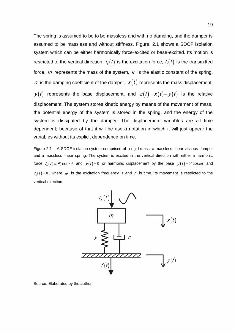
The spring is assumed to be to be massless and with no damping, and the damper is

assumed to be massless and without stiffness. Figure. 2.1 shows a SDOF isolation

system which can be either harmonically force-excited or base-excited. Its motion is

restricted to the vertical direction; ef t is the excitation force, t

f t is the transmitted

force, m represents the mass of the system, k is the elastic constant of the spring,

c is the damping coefficient of the damper, x t represents the mass displacement,

y t represents the base displacement, and z t x t y t is the relative

displacement. The system stores kinetic energy by means of the movement of mass,

the potential energy of the system is stored in the spring, and the energy of the

system is dissipated by the damper. The displacement variables are all time

dependent; because of that it will be use a notation in which it will just appear the

variables without its explicit dependence on time.

Figure 2.1 – A SDOF isolation system comprised of a rigid mass, a massless linear viscous damper

and a massless linear spring. The system is excited in the vertical direction with either a harmonic

force e ecosf t F t and 0y t or harmonic displacement by the base cosy t Y t and

0ef t , where is the excitation frequency is and t is time. Its movement is restricted to the

vertical direction.

Source: Elaborated by the author

20

2.2.1 Equations of Motion

Most of the work in this dissertation is mainly conducted in non-dimensional

variables, however some variables have dimension, mainly at the beginning of the

present chapter and at the beginning of Chapter 3. To avoid confusions in this sense,

it has been included a list of symbols with its dimensions in the first pages of this

dissertation.

In a linear system the viscous damping force is proportional to the relative

velocity between the ends of the damper and the elastic force of the spring is

proportional to the relative displacement between its ends. When the system is

excited by an external force, the base displacement is 0y and therefore z x .

The inertia of the body mf t , the spring force k

f t and the damping force df t act

in opposite direction to the excitation force ef t . This relation between the forces on

the system can be written as

m d k ef t f t f t f t

(2.1)

The harmonic excitation force has the form e ecosf t F t , where

eF is the

amplitude of the force, is the excitation frequency and t is the time. The force due

to the mass is mf t mx , the linear damping force is d

f t cx and kf t kx

is the elastic force of the spring. The overdot indicates differentiation in time, so that

x and x are the mass velocity and acceleration respectively, and the negative sign

indicates that inertia, damping and spring forces act in opposite direction of the

relative acceleration, velocity and displacement of the mass respectively. Using

Newton’s second law and substituting the previous definitions of the forces in Eq.

(2.1) the equation of motion of the force-excited system is given by

ecosmx cx kx F t

(2.2)

Note that the argument t is omitted here and in the remainder of this

dissertation for clarity. When the system is base-excited there are no excitation

21

forces 0ef and the force due to the mass depends only on the displacement x of

the mass, but the damping and stiffness forces depend on the relative displacement

z x y since the base is moving. Considering these conditions the equation of

motion for the base-excited system is given by

0mx c x y k x y

(2.3)

Subtracting my from both sides of Eq. (2.3), the equation of motion for the

base excited system can be expressed as a function of the relative displacement

mz cz kz my (2.4)

Equations (2.2) and (2.4) are the main equations describing the system shown

in Fig. 2.1 when is force-excited and base-excited. Equation (2.3) can be rearranged

so that the variables can be separated obtaining

mx cx kx cy ky (2.5)

Equation (2.5) will be useful further on when defining displacement

transmissibility in Section 2.3.

2.2.2 Transient, Steady-State and Resonance Frequency

The solutions for the system described by Eqs. (2.2) and (2.4) are composed

of the sum of two terms. The first term is the solution for the system when it vibrates

freely, which is known as the homogenous solution and represents a transient. This

is an oscillation at the natural frequency n

/k m which decays quickly in time

due to the damping present in the system. The second term is the particular solution

which represents the steady-state. This is a vibration in which the system oscillates at

the excitation frequency and lasts while the excitation force is active. In a physical

system, which is being excited by its base or by an external force, both kinds of

vibrations are present in the system oscillation but the transient always decays after

22

some time. The analysis on this work is based on the steady-state vibration of the

systems, so that the transient is not taken in account.

A resonant frequency is defined as the frequency for which the system

response is a maximum (Harris, 1961, p. 2-15), for the force and displacement

transmissibility it can be defined as the frequency for which the transmissibility is a

maximum. For low damping the resonance frequency of a system is very similar to its

natural frequency n

. Because of this, in this work the resonance frequency is

normalised by the natural frequency n

and the resonance frequency is assumed to

be when n

1/ .

2.3 Transmissibility for the linear isolator

The study on the linear and the nonlinear systems is conducted for two cases:

1) when the system is harmonically base-excited and 2) when the system is

harmonically force-excited. This is because in vibration isolation there are two

concerns: 1) to isolate a vibrating machine from its surroundings in order to reduce

the transmitted vibration from the machine to a receiver and 2) isolate a delicate item

of equipment from a vibrating host structure or base. Clearly the mass m represents

the mass of the machine or equipment and the damper and the spring are used to

reduce the transmission of movement or force. These elements together form the

isolator system.

2.3.1 Force and Displacement Transmissibility

Transmissibility is one of the most used concepts to measure the performance

of an isolator and is the concept used here to compare the performance between the

two systems analysed on this work. Transmissibility is defined as ratio of the

amplitude of the transmitted motion or force to the amplitude of the excitation motion

23

or force (Yan B. 2007, p. 3). When the system is being harmonically force-excited

( 0y and e ecosf t F t ) the force is transmitted through the spring and damper

to the receiver, thus the transmitted force is the sum of these two forces

tf t kx cx . Assuming a harmonic response and employing complex exponentials

to represent the excitation force e

j tF e , the transmitted force t

j tFe and the

displacement response j tx Xe , the amplitude of the transmitted force is

tF k j c X (2.6)

where 1j . Following the same process Eq. (2.2) becomes

2

ek m j cX F (2.7)

Combining Eqs. (2.6) and (2.7) results in the force transmissibility given by

t

F 2

e

F k j cT

F k m j c

(2.8)

When the system is base-excited the transmissibility is defined as the ratio of

the amplitude of the transmitted motion Y to the amplitude of the excitation motion

X . Using the complex representation for the excitation displacement j tx Xe and

the transmitted displacement j ty Ye , in Eq. (2.5) results in the displacement

transmissibility given by

D 2

Y k j cT

X k m j c

(2.9)

Note that force and displacement transmissibility for a linear system (Eqs.

(2.8) and (2.9) respectively) are equal. To obtain a non-dimensional expression for

the transmissibility, the numerator and the denominator of either Eqs. (2.8) or (2.9)

are divided by k . Noting that the damping ratio 2/n

c m , a non-dimensional

expression for the transmissibility can be determined. It is given by

F D 2

1 2

1 2

jT T

j

(2.10)

24

where /n

is the non-dimensional excitation frequency. Figure. 2.2 shows

force (and displacement) transmissibility for a SDOF isolation system described by

Eq. (2.10) for two different damping ratios representing low and high damping. The

results in Fig. 2.2 are shown in decibels, which is commonly used to specify

transmissibility as well as other physical quantities; it is a logarithmic quantity of the

ratio between two quantities, one of these being the reference quantity. The

transmissibility in decibels is defined as

1020 t

F D

e

logF

T dB T dBF

(2.11)

Figure 2.2 – Force and displacement transmissibility for a SDOF system with linear damping. Dashed

line - 0 01. , solid line - 0 1. , dashed dotted line - 21/ , dotted line - 0 01

2./ , straight solid

line - 0 1

2./ . It is possible to see that when the damping ratio is small enough - 0 01.

- there is a

frequency region d

2 in which transmissibility achieve the best case in vibration isolation for

this system (dB value ref. unity).

Source: Elaborated by the author

0.1 1 10 100-80

-60

-40

-20

0

20

40

= 0.01

= 0.1

1/2

20.01

/

20.1

/

Non-dimensional Frequency

|Tra

nsm

issib

ility

| dB

Isolation Region

From here

damper

starts to

dominate

for Damper starts

to dominate

for

25

It can be seen that at frequencies lower than I

2 , called the isolation

frequency, the transmitted force or displacement is generally higher than the

excitation force or displacement – this region is known as the amplification region. At

frequencies greater than I

2 the transmitted force or displacement is smaller

than the excitation force or displacement – this region is known as the isolation

region. It also can be seen that transmissibility at frequencies close the resonance is

determined by the amount of damping in the system; the larger the damping ratio the

smaller the transmissibility at the resonance. The effect of viscous damping has the

opposite effect in the isolation region. Increasing the damping ratio results in a

detrimental effect on the performance of the isolator, causing an increase in the

transmissibility in this region. There is a compromise in the choice of damping

between good control at resonance and good control at high frequencies (YAN B.

2007, p. 5). Finally Fig. 2.2 shows that at very low frequencies 1T , transmitted

force or displacement is equal to that of the excitation, which in decibels notation

corresponds to 0T dB .

Recalling that the numerator of Eq. (2.10) is the transmitted force and this

force is composed of the sum of the damping and the spring forces, it can be seen

that the term 2 j in the numerator is related to the damping force and the term 1

in the numerator is related to the spring force.

2.3.2 Transmissibility analysis for the linear system

Some analysis about transmissibility can be conducted by means of Eq.

(2.10). It is possible to find the frequency at which the force (or displacement) through

the damper starts to dominate the transmissibility. For this to happen the damping

force must to be equal to the force of the spring in the numerator of Eq. (2.10) then

1 2 j and the frequency at which the force through the damper starts to

dominate the transmissibility is d

1 2/ . To determine the transmissibility peak at

26

the resonance frequency, 1 is set in Eq. (2.10) and the largest terms remaining

are taken to obtain the value of transmissibility at resonance

F 1 D 1

1

2T T

(2.12)

From Eq. (2.12) can be seen what have been showed in Fig. 2.2, that an

increase in the damping results in a decrease in the transmissibility at the resonance

frequency. To determine the behaviour of transmissibility at high excitation

frequencies, d

is set in Eq. (2.10) and then the largest term in the numerator

and in the denominator are taken to obtain

F 1 D 1

2 T T

(2.13)

From Eq. (2.13) can be seen that far the resonance frequency an increase in

damping brings to an unfavourable effect increasing the transmissibility at this

frequencies. If the damping is low, which is the case when 0 01. so that the

frequency at which damping force starts to dominate the transmissibility become very

high compared with the isolation frequency d

2 the force through the spring

take account on transmissibility and then there is a frequency region d

2

where

F D 2

1T T

(2.14)

which is the best case which can be achieved in transmissibility for a SDOF system

(TANG; BRENAN, 2013). With low damping transmissibility decreases at a rate of

40dB per decade whilst with high damping transmissibility decrease at a rate of 20

dB per decade as showed in Fig 2.2.

27

2.4 Conclusions

In this chapter the most important features of a SDOF isolation system when it

is either excited by a harmonic force or is base-excited have been discussed. The

concept of transmissibility has been defined and used to measure the performance of

the system. This has provided a benchmark by which the performance of a nonlinear

isolator can be compared in Chapter 3. For the linear system it has been shown that

there are three regions in the transmissibility curve; the amplification region for

frequencies below I

2 , the region at which the transmissibility is mainly

dominated by the spring and the region at which the transmissibility is mainly

dominated by the damper. The last two regions are in the isolation region at

frequencies above I

. It has been shown that damping in the isolator has a

beneficial effect at frequencies close to the resonance frequency, but it has a

detrimental effect at high frequencies, where it increases the transmissibility.

28

3 NONLINEAR DAMPING ISOLATOR

3.1 Introduction

In Chapter 2 a SDOF isolation system has been studied. The main equations

describing the system when it is force and base excited has been shown. The

concept of transmissibility has been revised at different excitation frequencies and

presented as a mean by which the performance of the linear system can be

compared. In this chapter a SDOF system with a nonlinear damper is analysed. Its

performance is determined and the way in which the nonlinearity affects the internal

forces is investigated. To determine the performance of the system its force and

displacement vibration transmissibility are compared with that of a linear system

under harmonic force and harmonic base excitation. The study is conducted for both

small amplitude excitation, as it is possible to use analytical approximated

expressions, and for high amplitude excitation which is based on numerical

simulations.

This system is similar to the SDOF linear system described in Chapter 2. It is

also composed of a mass, a linear spring and a linear damper; but its damper is

placed so that it forms a 90º angle with the spring, as shown in Fig. 3.1. All the

nonlinear characteristics of the isolator are due to this geometrical configuration.

The system is excited in the direction of the spring and perpendicular to the

damper with either a harmonic force, when investigating the force transmissibility, or

harmonic displacement by the base, when investigating the displacement

transmissibility.

Tang and Brennan (2013) analysed this system with the purpose of

investigating the advantages of such a damper configuration for force and

displacement transmissibility. Here, part of this work is reproduced in detail to

compare its differences and advantages with that of a linear system, sometimes

using similar methods as employed by them and sometimes using other methods to

confirm their results.

29

Figure 3.1 – A SDOF system with damper oriented perpendicular to the spring (Horizontal damper

system). The system is excited in the vertical direction with either a harmonic force e ecosf t F t

and 0y t or harmonic displacement by the base cosy t Y t and 0ef t , where is the

excitation frequency and t is time. Its movement is restricted to the vertical direction.

Source: Elaborated by the author

3.2 Equations of motion

As the nonlinear characteristics of the system are due only to the geometric

configuration of the damper, it is necessary to determine the form of the damping

force in the direction of motion, in order to determine the equation of motion for the

system.

Figure 3.2 shows a free-body diagram of the damper. It can be seen that the

damping force in the vertical direction is given by d hsinf t F and the damper

length in any position by 2 2h a z , where hf t is the force produced by the

horizontal linear damper, hc is the horizontal linear damping coefficient, a is the

original damper length and z x y is the relative displacement between the mass

30

Figure 3.2 – Triangle formed by the horizontal damper in two different positions. The damper length is

a , the hypotenuse h corresponds to horizontal damper length in any position; is the angle formed

by the damper and the horizontal line, the relative displacement between the mass and the base is z ,

hc is the horizontal linear damping coefficient, the horizontal linear damping force is h

f t and the

nonlinear damping force produced by the horizontal damper in the vertical direction is df t .

Source: Elaborated by the author

and the base; when the system is force-excited, the base is stationary, so 0y , and

then z x (see Fig. 3.1).

According to Fig. 3.2 d hsinf t f t , expressing h

f t as the multiplication

of the relative velocity z and a damping coefficient which takes into account the

geometric properties of the damper in any position, and representing sin in terms of

z and a , a nonlinear expression of the damping force is obtained

2

2 2d h

zf t c z

a z

(3.1)

Note that unlike a linear damping force the nonlinear damping force depends

upon the amplitude of the relative displacement and not just upon the relative

velocity, hence the system nonlinearity is caused by this dependence. As discussed

by Tang and Brennan (2013), this kind of damping could be useful in situations in

which large damping is required for a large relative displacement, for example at

31

resonance, and low damping is required for a low relative displacement, for example

well-above the resonance frequency.

As the system is forced by ef t , the mass, or inertia, resists the change in

movement and then acts in opposite direction of ef t ; the stiffness and damping

forces act against the movement too. These relations can be written as

m d k ef t f t f t f t (3.2)

where mf t is the force due to the mass, d

f t is the damping force in the vertical

direction, kf t is the linear spring force. When the system is force-excited ( 0y ),

the harmonic excitation force is given by e ecosf t F t

and the stiffness and

damping forces are given by kf t kx and d h

f t c x respectively. Using

Newton’s second law and substituting the previous expressions for each force into

Eq. (3.2) gives the equation of motion for the force-excited system

2

h e2 2cos

xmx c x kx F t

a x

(3.3)

As discussed in Chapter 2, when the system is base-excited ( e0f t ) the

force due to the mass depends only on the displacement of the mass x , but the

damping and stiffness forces depend on the relative displacement z x y . The

corresponding equation of motion is then given by

2

h 2 20

zmx c z kz

a z

(3.4)

Subtracting my from both sides of the Eq. (3.4), the equation of motion for the

base-excited system becomes

2

h 2 2

zmz c z kz my

a z

(3.5)

Eqs (3.3) and (3.5) are the key equations describing the system shown in Fig.

3.1. Comparing Eqs. (3.3) and (3.5) with Eqs. (2.2) and (2.4), which are the main

32

equations describing the linear system, it can be seen that the difference is in the

nonlinearity present in the damping force of the nonlinear system. Eqs. (3.3) and

(3.5) can be solved using numerical methods, which is done in Section 3.4. However

some analysis is first conducted for low amplitudes of excitation. To do this some

approximations for the damping force have to be made.

3.3 Low Amplitude Excitation Study

When the relative displacement 0 2.z a the term 2z in the numerator of Eq.

(3.1) is small compared with 2a and can be neglected and this gives a simpler form

of the damping force, which is given by

2

d h 2

zf c z

a

(3.6)

The validity of this approximation is investigated by comparing the energy dissipated

by a damper with the actual damping force Eq. (3.1) and a damper with the

approximate damping force Eq. (3.6).

3.3.1 Energy Dissipated by a Damping Force

In general, the energy dissipated by a damping force for a damper alone, such

as that shown in Fig. 3.3, is given by the work done by the damping force (RUZICKA;

DERBY, 1971). Assuming a harmonic relative displacement sinz Z t , the energy

dissipated by the damping is four times the work done by the damping force over a

quarter of cycle of vibration, thus,

2

d

0

4/

E f zdt

(3.7)

33

Figure 3.3 – Schematic representation of a damper with equivalent viscous damping excited by a

harmonic force.

Source: Elaborated by the author

Substituting for z together with df given in Eq. (3.1) into Eq. (3.7), gives after some

manipulation, the energy dissipated by the damping force

2 22

2 4

h 2 2 2

0

4/ sin cos

sin

t tE c Z dt

a Z t

(3.8)

In order to obtain the approximate expression for the energy dissipated by the

damping z and Eq. (3.6) are substituting in Eq. (3.7), resulting

24

2 2 3

Approx. h 2

0

4/

cos cos cosZ

E c t t t dta

(3.9)

Using the trigonometric identity

3 3 3

4 4

cos coscos

t tt

(3.10)

It can be seen that for an excitation at frequency there is a response at this

frequency and at three times this frequency. If the response at only the excitation

frequency is considered (note that this is three times that of the third harmonic), then

Eq. (3.9) simplifies to

4

h

approx 24

c ZE

a

(3.11)

34

To compare the approximate energy dissipated by the damper given by Eq.

(3.11) and the actual energy dissipated given by Eq. (3.8), they are divided by the

energy dissipated by a linear damper 2

lE c Z (RAO, 2008, p. 70).

Setting hc c , where c is the linear viscous damping, and dividing Eqs. (3.8)

and (3.11) by lE , the normalised energy dissipated, which includes all the harmonics,

and the normalised energy approximated, which includes just the harmonic at the

excitation frequency, are respectively given by

2 222

2 2

0l

4

1

/ˆ sin cosˆ

sin

t tE ZE d tE Z t

(3.12)

and

2

Approx.4

ˆˆ ZE (3.13)

where ˆ /Z Z a . The expression for the actual damper given by Eq. (3.12) is

integrated numerically to give the normalised energy dissipated as a function of Z .

Figure 3.4 shows the normalised energy dissipated by the actual and the

approximate damping forces, given by Eqs. (3.12) and (3.13), as a function of the

relative displacement. It can be seen that both have similar behaviour - that of a

parabola, as they are dependent on 2Z , and that the lines begin to separate at the

point 0 2ˆ .Z . At this point the maximum error in the approximation for is only about

2%. Figure 3.5 shows the ratio of energy dissipated calculated using the approximate

expression to the actual energy dissipated in one cycle as functions of Z . It can be

seen that the energy calculated with the approximate expression is similar to the

energy calculated using the actual expression for the damping force. Thus, it can be

concluded that Eq. (3.6) is a good approximation to the damping force Eq. (3.1) for

values of 0 2.za as discussed by Tang and Brennan (2013).

35

Figure 3.4 – Non-dimensional energy dissipated. Solid line, energy calculated using the actual

damping force; dashed line, energy calculated using the approximated damping force.

Source: Elaborated by the author

Figure 3.5 –Ratio of actual energy dissipated to approximated energy dissipated. Solid line, energy

ratio calculated using the approximate damping force; dashed line, energy ratio calculated using the

actual damping force.

Source: Elaborated by the author

0 0.1 0.2 0.3 0.4 0.50

0.2

0.4

0.6

0.8

1

1.2

1.4

Approximation

Actual

0 0.1 0.2 0.3 0.4 0.50

0.01

0.02

0.03

0.04

0.05

0.06

0.07

0.08

0.09

0.1

Acutal

Approximation

0.19 0.195 0.2 0.205 0.21 0.2150.0085

0.009

0.0095

0.01

0.0105

0.011

0.0115

0.012

0.0125

0.013

Acutal

Approximation

Energ

y D

issip

ate

d

36

3.3.2 Equivalent Viscous Damping

It is possible to approximate the nonlinear damping forces Eqs. (3.1) and (3.6)

to equivalent linear viscous damping forces and thus represent the horizontal damper

system shown in Fig. 3.1 as the equivalent linear system shown in Fig. 3.6, by

employing the concept of equivalent viscous damping, such that Eqs. (3.1) and (3.6)

could be written as the multiplication of the equivalent damping coefficient and the

relative velocity d eqf c z .

Figure 3.6 – Schematic representation of a SDOF system with equivalent linear viscous damping

force. The system is excited in the vertical direction with either harmonic force ef and 0y or

harmonic displacement by the base y and e

0f . Its movement is restricted to the vertical direction.

Source: Elaborated by the author

As the interest in this section is the low amplitude transmissibility the

approximate damping force us used to obtain eqc . A similar process can be

conducted to obtain eqc for the actual damping force, however below it is shown that

there is an easier way to obtain it. According to Ruzicka and Derby (1971) to achieve

equivalence, between a nonlinear and a linear viscous damper, the energy dissipated

by the nonlinear damper in one vibration cycle should be equal to the energy

dissipated by a linear viscous damper for the same harmonic relative displacement.

37

It was shown in the last subsection that the damper with the approximate

damping force of Eq. (3.6), is valid for relative displacement values 0 2.za . The

equivalent viscous damping coefficient eqc can be determined by equating the

energy dissipated per cycle by the nonlinear damping element Eq. (3.11) to that

dissipated by the horizontal viscous damper 4 2 2

h eq4/c Z a c Z (RUZICKA;

DERBY, 1971), solving for eqc gives

22

eq h h2

1

4 4

ZZc c c

a (3.14)

which is the same as multiplying Eq. (3.13) by the horizontal viscous damping

coefficient hc . So to obtain

eqc for the actual damping force it is necessary simply

multiply Eq. (3.12) by hc , as

hc is a constant which multiplies both Eqs. (3.12) and

(3.13). Figure (3.4) can then be thought of as representing the behaviour of the

equivalent viscous damping coefficients as functions of Z , for the actual and the

approximate damping forces and Fig. (3.5) as representing its ratio as function of Z .

Now, it is possible to write the equation of motion for the harmonic force-excited

system Eq. (3.3) as

eq ecosmx c x kx F t (3.15)

and the equation of motion for the harmonically base-excited system Eq. (3.5), as

2

eqcosmz c z kz mY t (3.16)

where Y is the base displacement amplitude. Therefore the nonlinear system of Fig.

3.1 can be represented as the equivalent system in Fig. 3.6.

Equations. (3.15) and (3.16) can be expressed as dimensionless equations by

using the damping ratio and by defining some non-dimensional variables. The linear

damping ratio was defined in Chapter 2 as the ratio of the damping coefficient c

to the critical damping of the system, which is given by n

2m , where n

is the

natural frequency of the system. As hc is the horizontal viscous damping coefficient,

38

h

h

n2

c

m

represents the horizontal damping ratio. From Eq. (3.14) and the

previous the definitions, the equivalent damping ratio for the approximate system can

be written as

2

eq h

1

4Z (3.17)

Dividing Eqs. (3.15) and (3.16) by ka and using the non-dimensional force

e eˆ / ,F F a the amplitude of base displacement

ˆ / ,Y Y a the frequency

n

/ ,

the mass displacement ˆ / ,x x a

the relative displacement

ˆ / ,z z a and the non-

dimensional mass and relative velocities n

ˆ ' /z z a , n

ˆ ' /x x a , and

accelerations

2

nˆ '' /z z a ,

2

nˆ ' /x x a , which are obtained by differentiating x

and z in the non-dimensional time t n

, they can be written as

eq e2 ˆˆ ˆ ˆ'' ' cosx x x F (3.18)

2

eq2 ˆˆ ˆ ˆ'' ' cosz z z Y (3.19)

which are the general non-dimensional equations of motion for the harmonic force-

excited and the harmonic base-excited systems respectively. Note that eq

does not

necessarily come from the approximated expression to the damping force Eq. (3.17)

but can come from the actual damping force.

3.3.3 Transmissibility Equations for Low Amplitude Excitation

Force and displacement transmissibility were defined in Section 2.3 of

Chapter 2 as the ratio between the transmitted force to the excitation force and the

transmitted displacement to the base excitation, respectively. It was shown that in the

linear case force transmissibility is equals to displacement transmissibility. The force

is transmitted through the damper and the spring, however for the nonlinear system

the damping force has a different form, which leads to a different damping ratio. The

39

excitation force eˆ cosF can be written as the real part of a complex number

eˆ iF e

by employing the complex exponential, since cos sinje j . The use of

complex exponentials to represent the force makes the calculations easier because

the algebra is simpler. In the same way the mass, base and relative displacements

can be represented as complex numbers ˆˆ jx Xe , ˆ jy Ye and ˆˆ jz Ze

respectively. Substituting the complex forms of the excitation force and

displacements, and Eq. (3.17) in Eq. (2.10) from Chapter 2, the force and

displacement transmissibility for the nonlinear system are given by

2

h

F 22

h

11

21

12

ˆ

ˆ

j XT

j X

(3.20)

h

D

h

ˆ

ˆ

j ZT

j Z

2

22

11

21

12

(3.21)

Note that unlike the linear system, for the nonlinear damper system the force

and displacement transmissibility are not the same. This is because for the nonlinear

system the damper force depends on the square of the relative displacement which is

ˆ ˆ ˆZ X Y for the base excited system and ˆ ˆZ X for the force excited system.

In order to obtain the transmissibility at each frequency of excitation it is necessary to

know the displacement and relative displacement at this frequency. These are given

by

ˆ

ˆ

ˆ

eF

X

j X

2

2

h

11

2

(3.22)

2

22

h

11

2

ˆˆ

ˆ

YZ

j Z

(3.23)

In Eqs. (3.22) and (3.23) the unknown variable is a function of itself. Tang and

Brennan (2013) used the harmonic balance method (HBM) to determine X and Z

40

and have suggested that Eqs. (3.22) and (3.23) can be solved iteratively. Here,

another solution method is used.

3.3.4 Solution of Transmissibility Equations (Low Amplitude Excitation)

Note that the transmissibilities given in Eqs. (3.20) and (3.21) are not

dependent on the complex displacement amplitude but the absolute value of

displacement amplitude and that Eqs. (3.22) and (3.23) are complex functions and

therefore they can be represented in the form j , where is a complex

number, is the real part and the imaginary part of . It is thus possible to find

X and Z by analogy to finding the absolute value of a complex number, that is

, where is the conjugate of .

Multiplying the right side of Eq. (3.22) by its denominator and then separating

the result in its real and imaginary parts leads to

e he

h h

22

2 22 22 2

2 2

11

2

1 11 1

2 2

ˆ ˆˆˆ

ˆ ˆ

F XFX j

X X

(3.24)

For the force-excited system to obtain X it is just necessary to multiply X by

its conjugate and take the root square of the result, which can be written as

12 2 2

22

e he

2 22 22 2

2 2

h h

11

2 01 1

1 12 2

ˆ ˆˆˆ

ˆ ˆ

F XFX

X X

(3.25)

One way to determine the value of X for every frequency is to search for

the value of X for which Eq. (3.25) is satisfied. Once a value of X is obtained this

41

is used in Eq. (3.20) to determine a value of transmissibility for every and then the

process is repeated for the next frequency . Such a procedure is used for the

base-excited system as well, and the equation from which Z is obtained is

12 2 2

22 2

h

2 22 22 2

2 2

h h

11

2 01 1

1 12 2

ˆ ˆˆˆ

ˆ ˆ

Y ZYZ

Z Z

(3.26)

In Fig. 3.7 are shown the force and displacement transmissibilities for the

nonlinear isolator system when 0 4ˆ .eF and ˆ .Y 0 4 respectively with

h 10 ,

Figure 3.7 – Force and displacement transmissibility when ˆ .F e

0 4 and 0 4ˆ .Y respectively for

the nonlinear isolator system with h

10 . Solid line - displacement transmissibility, dashed line -

linear isolator with 0 1. , dotted line - force transmissibility, dashed dotted line: 21/ (dB value ref.

unity)

Source: Elaborated by the author

0,1 1 10 100-80

-70

-60

-50

-40

-30

-20

-10

0

10

20

Trans Linear Isol. = 0.1

1/2

Disp. Transm. Horiz. Isol.

F. Transm. Horiz. Isol.

Non-dimensional Frequency

|Tra

nsm

issib

ility

| dB

30 100-80

-60

Non-dimensional Frequency

|Tra

nsm

issib

ility

| (d

B)

Force and Displacement Transmissibility for Horizontal Damper System

Isolation

region

42

obtained using the method described above. The transmissibility of a linear isolator

with 0 1. is also shown for comparison. These results are similar to those

presented by Tang and Brennan (2013) who used the HBM to obtain their results.

3.3.5 Transmissibility Analysis (Low Amplitude Excitation)

Some analysis can be conducted on Eqs. (3.20), (3.21), (3.22) and (3.23) with

the purpose of predicting the force and displacement transmissibilities in the different

frequency regions for displacement amplitudes less than or equal to 0 2. a . To

determine the behaviour of transmissibility for the harmonic force-excited system for

high excitation frequencies, 1 in Eq. (3.22) is considered and then the largest

terms in the numerator and in the denominator are taken to give

2

emax 1

ˆ ˆ /X F

.

Substituting this result in Eq. (3.20) and taking the largest terms yields

2

e

h 3

F 2212 e

h 3

11

12

11

2

ˆ

ˆ

Fj

TF

j

(3.27)

This results shows that at high frequencies the nonlinear isolator is very

effective as the displacement amplitude does not depend on damping. Thus, the

force through the damper become practically zero at high frequencies compared with

the force through the spring and then the system behaves as it were undamped,

which is the best that can be achieved for a SDOF system (see Fig. 3.7).

For the resonance region 1 , 1 3

e h1

2/

ˆ ˆ /X F

, and the transmissibility

at resonance is given by

23F h e1

2 ˆ/T F

(3.28)

In order to maintain the transmissibility peak at resonance of the nonlinear

isolator equal to or less than that of the linear isolator, the inequality

43

1 3

2

h e2 1 2

/ˆ/ /F

must be satisfied, which means that to achieve this

3

e h4ˆ /F . That is, if the excitation force is less than this value the nonlinear

isolator peak at resonance will be greater than the resonance peak of the linear

system. Consequently the performance will be worse than that of the linear isolator.

This is because the damping force produced by the horizontal damper is large when

the relative displacement is large, and the fact that the isolator behaves as if it is

undamped at high frequencies is because the damping force is small when the

relative displacement is small.

According to Eq. (3.28), and what has been mentioned previously, the

resonance peak of the force transmissibility for the nonlinear isolator will decrease as

the excitation force ˆeF increases. This is a desirable effect, but it should be noted

that this is valid only for displacement values less than 0 2. a . Taking into account this

restriction and setting 1 on Eq. (3.22), a limit on the excitation force is found to

be 250ˆ /e hF .

A similar procedure is conducted when the isolator is harmonically base-

excited. For high frequencies the upper limit of the relative displacement

max

ˆ ˆZ Y

1

is found and then the displacement transmissibility becomes

22

hh

D 12 2

h

11

21 2

12

ˆ ˆ

ˆ

j Y YT

j Y

(3.29)

Note that at high frequencies there is a detrimental effect on the displacement

transmissibility for the base-excited isolator when compared with the force-excited

isolator as shown in Fig. 3.7. This effect is similar to that produced by a linear isolator

where the force and displacement transmissibilities are proportional to 1/ .

Equating the terms in the numerator of Eq. (3.29) the frequency value at which the

force through the damper starts to dominate the transmissibility in the nonlinear

isolator can be found, this is given by 2

d h2 ˆ/ Y . At frequencies lower or equal to

d but inside the isolation region, it is the force through the spring which mainly

44

dominates the transmissibility and then for these values the transmissibility is

proportional to 21/ . In order to obtain a better performance than the linear isolator,

d for the nonlinear isolator should be higher than

d for the linear isolator, that is

2

h2 1 2ˆ/ /Y and from this provided that h

2ˆ /Y the frequency range for

which the displacement transmissibility is proportional to 21/ will be extended and

will be larger than the corresponding range for the linear isolator.

At the resonance frequency, and from Eq. (3.23), the limit for the relative

displacement is h

1 3

12

/ˆ ˆ /Z Y

, substituting this value into Eq. (3.21) and

Table 3.1 Important values for the linear and the nonlinear horizontal damper isolators valid for

displacement amplitudes less or equal to 0 2. a .

Force-excited

Base-excited

Linear viscous Damper

Horizontal linear viscous damping

Linear viscous Damper

Horizontal linear viscous damping

Amplitude of relative

displacement at resonance

1

X

or 1

Z

e2ˆ /F

/

ˆ /1 3

2 e hF 2ˆ /Y 1 3

h2

/ˆ /Y

Amplitude of transmissibility at

resonance

F 1T

or

D 1T

1 2/ 1 3

2

h e2

/ˆ/ F 1 2/

1 32

h2

/ˆ/ Y

Amplitude of transmissibility at high

frequencies

F 1T

or

D 1T

2 /

21/ 2 / 2

h2ˆ /Y

Frequency at which the

damping force starts to

dominates d

1 2/ 1 2/ 2

h2 ˆ/ Y

Minimum force or base

displacement - 3

h4 / - 3

h4 /

Maximum force or base displacement - h

250/ - h250/

Ratio of maximum to

minimum force or base displacement

-

3 2

3h 10

/

-

3 2

3h 10

/

Isolation frequencyI

2 2 2 2

Source: Adapted from Bing Tang and Brennan (2013)

45

manipulating the subsequent expression, the displacement transmissibility of the

nonlinear system at resonance becomes

ˆ/T Y

23D h1

2 (3.30)

For the nonlinear isolator to have a better performance than the linear isolator,

the inequality 1 3

2

h2 1 2

/ˆ/ /Y should be satisfied. This means that the amplitude

of the base displacement should be h

34ˆ /Y . As the relative displacement

amplitudes have a limiting value of . a0 2 , similar to that for the force-excited system,

it leads to the restriction h

250ˆ /Y (see Fig. 3.7). The important values from this

analysis for the linear and the non-linear isolator are shown in Table 3.1

As e h

250ˆ /F and if 0 1. and h

10 then the maximum allowable value

for the excitation force is e

0 4ˆ .F , and then the maximum allowable base

displacement amplitude for the base excited system is 0 4ˆ .Y . These are the

values used in the plots to try and show the maximum effect.

3.4 Transmissibility for High Amplitude Excitation

When the amplitude of excitation for the nonlinear isolator is such that the

relative displacement is higher than 0 2. a the results from the previous study of

Section 3.3 cannot to be applied and then it is necessary to return to the actual form

of the equations of motion Eqs (3.3) and (3.5) which can be written in dimensionless

form as

2

h e22

1

ˆ ˆˆ ˆ ˆ'' ' cosˆ

xx x x F

x

(3.31)

22

h 22

1

ˆ ˆˆ ˆ ˆ'' ' cosˆ

zz z z Y

z

(3.32)

46

To calculate the force and displacement transmissibility for high excitation

amplitudes from Eqs. (3.31) and (3.32) the system is excited at single frequencies.

The time responses of the system x and z are obtained by solving the differential

equations by means of the fourth-order Runge-Kutta method at each excitation

frequency, employing the Matlab function Ode45. The transients are discarded,

since the principal interest is on responses at the excitation frequencies and at three

times this frequency. From the steady state responses their maximum amplitudes are

taken to calculate the forces through the spring and the damper, which correspond to

the second and the third terms on the left sides of Eqs. (3.31) and (3.32). They are

then summed and divided by the excitation force amplitude, which is known, to obtain

the force transmissibility for high amplitude excitation.

A similar equation is obtained for the displacement transmissibility. Once a

transmissibility value has been determined for one frequency the process is repeated

for the next frequency, with a small increment in frequency, until the whole frequency

range is covered.

Force transmissibilities for different values of excitation amplitudes are shown

in Fig 3.8. It is possible to see that for high levels of excitation the nonlinear system

behaves very well at high frequencies, still as if were undamped, but at frequencies

close to resonance the transmissibility is affected badly by the nonlinearity of the

damping force, although the transmissibility at the resonance frequency remains

smaller than for the linear system. Tang and Brennan (2013) have shown that the

nonlinear damping force distorts the time histories of the force transmissibility

resulting in a response which contains higher order harmonic terms, and that this

effect is proportional to the excitation amplitude. In the next chapter this effect is

studied in detail.

In Fig. 3.9 the displacement transmissibility of the nonlinear isolator for

different values of high amplitudes of excitation is shown. It is possible to see that at

resonance and close to it, the system performs even better than for low excitation

levels but at high frequencies the displacement transmissibility of the system

increases and for some values of excitation this effect is worse than for the linear

47

Figure 3.8 – Force transmissibility for the nonlinear isolator system with 0 1. and h

10 . For:

solid line - linear isolator, dashed line - e

0 1ˆ .F , dashed dotted line - e

0 2ˆ .F , dotted line - e

0 3ˆ .F

and dashed line - e

0 5ˆ .F (dB value ref. unity).

Source: Elaborated by the author

system. This is due to the relation between the frequency at which the damping force

starts to dominate the transmissibility and the excitation amplitude, established in the

last section ( 2

d h2 ˆ/ Y ).

Directly from Fig 3.9 can be seen that depending on the situation, the

transmissibility at high frequencies can be reduced be reducing h

and accepting

some detrimental effect at resonance. As Tang and Brennan (2013) mention, this

also occurs with the linear system, as there is a trade-off between reducing the

response at resonance and increasing the transmissibility at higher frequencies.

.1 1 10-40

-20

1

20

Linear System

Fe = 0.1

Fe = 0.2

Fe = 0.3

Fe = 0.5

Non-dimensional Frequency

| F

orc

e T

ransm

issib

ility

| dB

48

Figure 3.9 – Displacement transmissibility for the nonlinear isolator system when 0 1. and h

10 .

For: solid line - linear isolator, dashed line - e

0 1ˆ .Y , dashed dotted line -e

0 2ˆ .Y , dotted line -

e0 3ˆ .Y and dashed line

e0 5ˆ .Y (dB value ref. unity).

Source: Elaborated by the author

3.5 Conclusions

In this chapter it has been shown that the nonlinear damping force produced

by a horizontal damper which is perpendicular to the spring force and to the

movement direction in an isolator, can be approximated by an equivalent linear

viscous damping force, for low displacement amplitudes, without there being a

considerable difference in the energy dissipated. Also, this nonlinear damping force is

proportional to the square of the relative displacement amplitude between the mass

and the base. This is beneficial for a vibration isolator as the damping force is large

when the amplitude is large and small when the amplitude is small.

.1 1 10-40

-20

1

20

Linear System

Ye = 0.1

Ye = 0.2

Ye = 0.3

Ye = 0.5

Non-dimensional Frequency

|Dis

pla

cem

ent

Tra

nsm

issib

ility

| dB

49

When the system is excited with low amplitudes it was found that at the

resonance frequency its force and displacement transmissibilities are lower than for

the linear isolator and therefore the nonlinear system performs better than the linear

system, but there are conditions on the minimum amplitudes of force and

displacement excitation below which the nonlinear system will perform worse than

the linear system (see Table 3.1). At frequencies when 1 it was shown that with

respect to the force transmissibility, the nonlinear isolator performs better than the

linear isolator as the force transmitted through the damper is negligible compared

with the force transmitted to the spring and the system behaves as if it were

undamped. Concerning the displacement transmissibility of the nonlinear system it

was found that it perform betters than the linear system but there is a detrimental

effect as it depends on 1/ (see Table 3.1).

When the system is excited with a high amplitude it was shown that for the

force transmissibility the nonlinear isolator at resonance performs better than the

linear system, but close to the resonance there is an unfavourable effect which

increases the transmissibility at these frequencies. It also was shown that at

frequencies when 1 the force transmissibility of the nonlinear system is very

good since the system behaves as if it were undamped. Concerning the

displacement transmissibility, at resonance the nonlinear isolator performs better

than the linear isolator, but the frequency at which the damper begins to dominate

the transmissibility decreases with the excitation amplitude. At high excitation

amplitude this results in a detrimental effect on the displacement transmissibility.

50

4 DETAILED ANALYSIS OF THE NONLINEAR

ISOLATION SYSTEM

4.1 Introduction

In the previous chapter it was shown that the force transmissibility of the

nonlinear damping system has desirable characteristics at high frequencies. However

at frequencies close to the resonance frequency, the system has undesirable

characteristics, even though the peak at resonance is smaller than that of the linear

system (see Fig. 3.8). In this chapter an investigation is carried out into the causes of

these adverse effects. The time histories of the internal forces are decomposed into

their spectral components using the Fourier series in the resonance region, and

these are studied to determine the sources of the nonlinearities and the way in which

they propagate through the system.

4.2 Brief Review of the Fourier series

The time histories for the transmitted forces and its components are periodic

which repeats every period of the excitation frequency 2 /T , where is the

excitation frequency, see for instance Fig. 4.1. Periodic signals can be analysed

using the Fourier series. A periodic signal can be represented by adding together

sine and cosine functions of appropriated frequencies, amplitudes and relative

phases (SHIN; HAMMOND, 2008, p 31).

The Fourier series representation of a periodic signal is given by (Shin and

Hammond, 2008, p 312)

0

n nn 1

2 2

2cos sin

a nt ntx t a b

T T

(4.1)

51

where 1 2 3 4 , , , , ...n and the fundamental frequency, which corresponds here to

the excitation frequency is 2 /T , and the higher frequencies are integers

multiples of this. The amplitudes of the higher frequencies than the fundamental are

called harmonics. The quantity 0

2/a is the mean value of the signal and the

coefficients na and

nb are the Fourier coefficients which are used to calculate the

amplitude and the phase of each harmonic as follows:

2 2

n

1

n n ntan /

n nA a b

b a

(4.2)

where nA is the amplitude of the nth harmonic and

n its phase angle. The Fourier

series representation in terms of the amplitudes and the phase is given by

0

n nn 1

22

cosa

x t A n

(4.3)

The Fourier coefficients are calculated from (Shin and Hammond, 2008, p 32)

0

0

n

0

n

0

1

2

2 2 n = 1, 2, 3,...

2 2

cos

sin

T

T

T

ax t dt

T

nta x t dtT T

ntb x t dtT T

(4.4)

The amplitudes and the frequencies are used to create the spectrum of the

signal to determine the influence of each harmonic in the original signal. Depending

on the signal it can be composed by odd or even harmonics or a combination of the

two.

4.3 Study of the harmonic content of the signals

In this section the Fourier series is used to analyse the transmitted force in the

resonance region as there is undesirable behaviour in this region, see Fig. 3.8. The

52

resonance region is roughly the frequency 0 3 1 6. . so the present study will

focus on the transmitted force at these frequencies. Taking in account the fact that

the damping force is the cause of the nonlinearity of the system, as shown in Eq.

(3.31), it is thought that this is the cause of the adverse behaviour. Tang and

Brennan (2013) made the following comment:

The nonlinear damping force has a profound effect on the transmissibility

response and the time history response at the excitation frequency. The

nonlinear damping force distorts the time history curves of the force

transmissibility with the undesirable result that there are many high order

harmonic terms in the response. The larger the excitation force amplitude,

the stronger the influence on the force transmissibility curves (Tang and

Brennan, 2013, p. 517).

Following this indication the time history for the transmitted force as well as its

frequency spectrum at different excitation frequencies in the resonance region are

analysed. As the transmitted force is composed of the force transmitted by the spring

and the force transmitted by the damper, the time histories of those forces with their

frequency spectra are compared and analysed to determine the influence of each

one of this forces on the transmitted force. Using the definition of the damping force

from Eq. (3.31) and setting z x , the damping force is decomposed into the velocity

of the mass ˆ 'x and the damping coefficient fc which has the form

2

f 22

1

ˆ

ˆh

xc

x

(4.5)

Hence the damping force can be written as d f

ˆ 'f c x . The time history of the

damping coefficient and the velocity as well as its frequency spectra are also

analysed with the aim to determine the influence of each of them on the nonlinearity

of the damping force. This procedure is conducted for the nonlinear system when

excited at five different frequencies; the first four of them are in the resonance region:

0 3. , 0 5. , 1 , 1 5. , while the last one belongs to the beginning of the

isolation region: 2 .

53

4.3.1 Spectrum of the Transmitted Force

From Eq. (3.31) can be obtained the expression for the non-dimensional

transmitted force 2

h 22

1

ˆˆ ˆ ˆ'ˆt

xf t x x

x

, Composed by the force transmitted through

the damper and the force transmitted through the spring, respectively. The non-

transmitted force is composed of non-dimensional expression; therefore in this

section the transmitted forces through the spring and the damper, as well as the total

transmitted force are all non-dimensional forces. Also the velocity and the nonlinear

damping coefficient are non-dimensional variables.

To demonstrate the effect of the external excitation on the nonlinear system,

the maximum value of the force in Chapter 3 is used, i.e., e

0 5ˆ .F , and the horizontal

damping coefficient h

10 .

Figure 4.1 shows the time histories for the force transmitted through the

nonlinear isolation system for the excitation frequencies 0 3. , 0 5. , 1 ,

1 5. and 2 , together with their respective frequency spectra. Figs. 4.1 (a)

and (b) show the time history for the transmitted force at 0 3. and its frequency

spectrum respectively; the harmonics shown in Fig. 4.1 (b) with the mean value (DC

value) at zero frequency are used to reconstruct the original transmitted force curve

in Fig 4.1 (a) by means of the Fourier series. This reconstruction, which serves to

validate the frequency spectrum, is overlaid on the original curve. In Fig 4.1 (a) the

first harmonic is also plotted which represents the transmitted force at the excitation

frequency and which closely follows the transmissibility curve, and the excitation

force, which has an amplitude e

0 5ˆ .F .

There can be seen that at this low frequency the maximum value of the

transmitted force reaches nearly three times the amplitude of the excitation force, the

presence of higher order harmonics can also be seen, which makes the transmitted

force larger than the amplitude of first harmonic. Figure 4.1 (b) reveals that it only odd

harmonics are needed to reconstruct the transmitted force curve and that the most

important influence in the transmissibility is the force transmitted at the excitation

54

Figure 4.1 - Time history for the non-dimensional transmitted force through the nonlinear isolation

system and its frequency spectrum when h

10 and e

0 5ˆ .F for a) 0 3. , c) 0 5. , e) 1 , g)

1 5. , i) 2 . Blue solid line – time history for the transmitted force, yellow dotted line – Fourier

series of the time history, red dashed line – first harmonic of the Fourier series, black solid line –

excitation force, magenta horizontal line – mean value (DC level) of the signal. b), d), f) h) and j) –

Frequency spectrum with the DC value at zero and the first fifteen harmonics from the Fourier series

of the time history for the transmitted force curves shown in a), c), e), g), and j).

0 0,5 1 1,5 2

-2

-1.5

-1

-0.5

0

0.5

1

1.5

2

0 1 3 5 7 9 11 13 150

0.2

0.4

0.6

0.8

1

1.2

1.4

DC value - At Zero

0 1 3 5 7 9 11 13 150

0.2

0.4

0.6

0.8

1

1.2

1.4

DC value - At Zero

0 0.5 1 1.5 2

-1

-0.5

0

0.5

1

Harmonics Frequency

a) b)

Tra

nsm

itte

d F

orc

e

Non-dimensional time

Am

plitu

de

0 1 3 5 7 9 11 13 150

0.2

0.4

0.6

0.8

1

1.2

1.4

DC value - At Zero

c) d)

Tra

nsm

itte

d F

orc

e

Am

plitu

de

0 0,5 1 1,5 2

-2.5

-2

-1.5

-1

-0.5

0

0.5

1

1.5

2

2.5

e) f)

Harmonics Frequency

Tra

nsm

itte

d F

orc

e

Non-dimensional time

Am

plitu

de

Non-dimensional time Harmonics Frequency

55

0 0,5 1 1,5 2

-1

-0.5

0

0.5

1

0 1 3 5 7 9 11 13 150

0.1

0.2

0.3

0.4

0.5

0.6

0.7

0.8

0.9

DC value - At Zero

g) h)

Harmonics Frequency

Tra

nsm

itte

d F

orc

e

Non-dimensional time

Am

plitu

de

0 1 3 5 7 9 11 13 150

0.05

0.1

0.15

0.2

0.25

0.3

0.35

DC value - At Zero

Harmonics Frequency

0 0,5 1 1,5 2

-0.4

-0.3

-0.2

-0.1

0

0.1

0.2

0.3

0.4

0.5

Am

plitu

de

j

Non-dimensional time

i)

Tra

nsm

itte

d F

orc

e

Source: Elaborated by the author

frequency (1st harmonic). Its amplitude is nearly 80% of the maximum value of the

transmitted force curve. The force transmitted at the excitation frequency is more

than twice the amplitude of the excitation force; the influence of the force at three,

five, seven and nine times the excitation frequency is not so large but does adversely

affect the transmitted force. Harmonics higher than the 9th have a negligible influence

on the transmissibility.

When the system is excited with a frequency 0 5. , (see Figs 4.1 (c) and

(d)), the transmitted force increases considerably being nearly five times the

amplitude of the excitation frequency; the influence of the force transmitted at the

excitation frequency continues to be significant since is nearly half of the total

transmitted force is transmitted by the first harmonic. Comparing Fig. 4.1 (b) and (d)

can be seen that the amplitude of the first harmonic is almost the same as for

0 3. unlike the amplitudes of the 3rd, 5th, 7th and 9th harmonics which are larger

for 0 5. than for 0 3. .

56

When the system is excited at resonance 1 , which is illustrated in Figs.

4.1 (e) and (f), the transmitted force increases just a little compared with the

excitation force at 0 5. , its maximum value is five times greater than the

amplitude of the excitation force. The transmitted force at the excitation frequency is

still nearly half of the total transmitted force. Unlike the frequency spectrum of the

transmitted force at 0 5. Fig. 4.1 (f) shows a significant contribution of the

transmitted force mainly at three times and five times the excitation frequency and to

a lesser extent at seven times the excitation frequency. The influence of harmonics

higher than the 7th can be neglected. The time history of the transmitted force at the

resonance has a slightly different shape than at lower frequencies, having its

maximum and minimum values greater than the maximum and minimum of the 1st

harmonic and the excitation force. At 1 5. the transmitted force decreases, again

its maximum value is nearly three times the amplitude of the excitation force. This is

illustrated in Figs. 4.1 (g) and (h), where it can be seen that the transmitted force is

mainly composed of the 1st and the 3rd harmonic, and to some extent, the 5th

harmonic. There is no influence of harmonics higher than the 5 th in the time history of

the transmitted force.

In the isolation region at 2 the force transmitted is, as expected, less than

the amplitude of the excitation force and is composed of the 1st and the 3rd harmonic,

see Figs. 4.1 (g) and (h). There is no influence of harmonics higher than the 3rd. The

amplitude of the first harmonic is nearly 70% of the amplitude of the transmitted

force. The transmitted force at this excitation frequency starts to be similar to a sine

wave.

4.3.2 Force Through the Spring

As mentioned previously the total transmitted force to the base consists of the

force transmitted through the spring and the force transmitted through the damper. In

order to establish what is the importance of each component on the transmitted force

in this subsection, the time history for the force transmitted through the spring and its

frequency spectrum are studied. As in the previous section the frequencies 0 3. ,

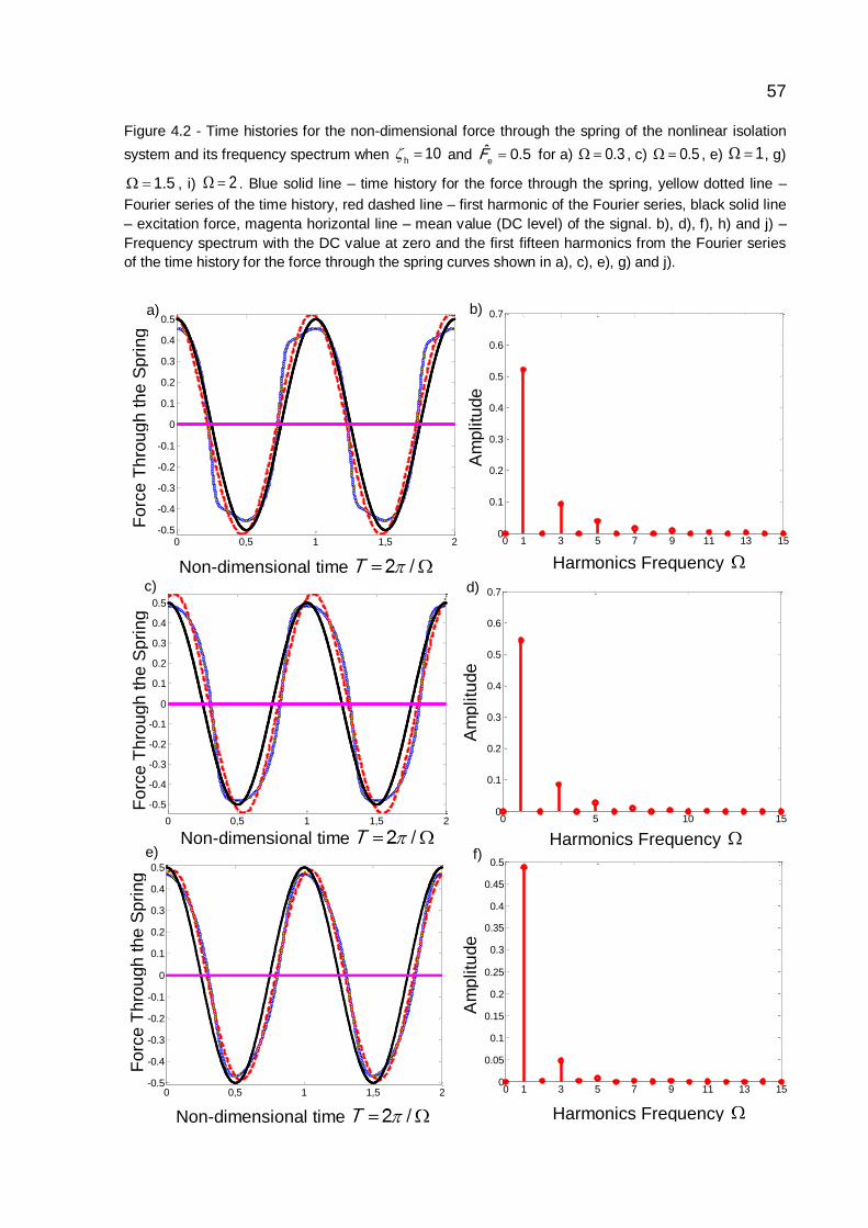
57

Figure 4.2 - Time histories for the non-dimensional force through the spring of the nonlinear isolation

system and its frequency spectrum when h

10 and e

0 5ˆ .F for a) 0 3. , c) 0 5. , e) 1 , g)

1 5. , i) 2 . Blue solid line – time history for the force through the spring, yellow dotted line –

Fourier series of the time history, red dashed line – first harmonic of the Fourier series, black solid line

– excitation force, magenta horizontal line – mean value (DC level) of the signal. b), d), f), h) and j) –

Frequency spectrum with the DC value at zero and the first fifteen harmonics from the Fourier series

of the time history for the force through the spring curves shown in a), c), e), g) and j).

0 0,5 1 1,5 2-0.5

-0.4

-0.3

-0.2

-0.1

0

0.1

0.2

0.3

0.4

0.5

0 0,5 1 1,5 2-0.5

-0.4

-0.3

-0.2

-0.1

0

0.1

0.2

0.3

0.4

0.5

0 1 3 5 7 9 11 13 150

0.1

0.2

0.3

0.4

0.5

0.6

0.7

DC value - At Zero

Harmonics Frequency

a) b)

Fo

rce

Th

rou

gh

th

e S

pri

ng

Non-dimensional time

Am

plitu

de

0 0,5 1 1,5 2

-0.5

-0.4

-0.3

-0.2

-0.1

0

0.1

0.2

0.3

0.4

0.5

0 5 10 150

0.1

0.2

0.3

0.4

0.5

0.6

0.7

DC value - At Zero

Non-dimensional time

Am

plitu

de

c) d)

Fo

rce

Th

rou

gh

th

e S

pri

ng

0 1 3 5 7 9 11 13 150

0.05

0.1

0.15

0.2

0.25

0.3

0.35

0.4

0.45

0.5

DC value - At Zero

Fo

rce

Th

rou

gh

th

e S

pri

ng

Harmonics Frequency

Am

plitu

de

Non-dimensional time

e) f) Harmonics Frequency

58

Source: Elaborated by the author

0 5. , 1 , 1 5. and 2 are considered. There is another important point

to be made. The non-dimensional force through the spring corresponds to the third

term in the left side of Eq. (3.31). It is equal to the non-dimensional displacement, so

the force through the spring and the displacement of the mass have the same

behaviour.

Figure 4.2 shows the time histories for the force transmitted through the spring

together with their respective frequency spectra at five different frequencies; four of

which are in the resonance region and the other one corresponds to the beginning of

the isolation region. Figures 4.2 (a) and (b) shows the force transmitted through the

spring when the system is excited at 0 3. and its frequency spectrum, it can be

seen that the amplitude of the force is a little smaller than the amplitude of the

excitation force and is mainly composed of the 1st and to a lesser degree the 3rd

harmonic. This feature maintains when the system is excited at 0 5. (see Figs.

4.2 (c) and (d)) and 1 (Figures. 4.2 (e) and (f)), in which the amplitude of the

0 0,5 1 1,5 2

-0.4

-0.3

-0.2

-0.1

0

0.1

0.2

0.3

0.4

0.5

0 1 3 5 7 9 11 13 150

0.05

0.1

0.15

0.2

0.25

0.3

0.35

DC value - At Zero

0 0,5 1 1,5 2

-0.4

-0.3

-0.2

-0.1

0

0.1

0.2

0.3

0.4

0.5

Harmonics Frequency

Fo

rce

Th

rou

gh

th

e S

pri

ng

Am

plitu

de

0 1 3 5 7 9 11 13 150

0.02

0.04

0.06

0.08

0.1

0.12

0.14

0.16

0.18

DC value - At Zero

Am

plitu

de

Fo

rce

Th

rou

gh

th

e S

pri

ng

Harmonics Frequency

Non-dimensional time

g)

Non-dimensional time

h)

i) j)

59

force through the spring is smaller but almost equal to the amplitude of the excitation

force. The time histories are slightly distorted mainly by the small influence of the 3 rd

harmonic and the negligible 5th harmonic. They are very similar to the sine wave

representing the excitation force. Thus at frequencies less than or equal to the

resonance frequency, the force transmitted through the spring is almost equal to the

amplitude of the excitation force. It also can be seen that the displacement of the

mass is only slightly distorted when the system is excited at frequencies below the

resonance frequency.

Figures. 4.2 (g) and (h) shows the transmitted force through the spring at

1 5. and its frequency spectrum. It can be seen that the amplitude of the force

transmitted through the spring decreases, it is nearly 70% of the amplitude of the

excitation force and is basically composed of the 1st harmonic. When the system is

excited at 2 , the amplitude of the force transmitted through the spring is nearly

30% the amplitude of the excitation force. This is illustrated in Figs 4.2 (i) and (j). So

at frequencies higher than the resonance frequency the transmitted force becomes

sinusoidal and the force transmitted through the spring decreases.

4.3.3 Force through the Damper

Figure 4.3 shows the time history for the force through the damper and its

frequency spectrum for 0 3. , 0 5. , 1 , 1 5. and 2 . Also shown is

the time history of the first harmonic, the excitation force and the mean value. Again,

it can be seen that only odd harmonics are needed to reconstruct the original curve.

Figures. 4.3 (a) and (b) shows the time history and the frequency spectrum of the

force through the damper at 0 3. ; it can be seen that the peak value of the

transmitted force is less than the amplitude of the excitation force being nearly 80%

of this amplitude. Figure 4.3 (b) displays an interesting frequency spectrum. The

force transmitted at the excitation frequency is nearly half the amplitude of the

excitation force but unlike almost all the previous frequency spectra, the harmonics

higher than the fundamental frequency do not decrease as the frequency increases.

The 3rd harmonic is very small and the 5th, 7th, 9th, 11th 13th have a considerable

amplitude and it is mainly these that compose the other part of the transmitted force.

60

0 1 3 5 7 9 11 13 150

0.02

0.04

0.06

0.08

0.1

0.12

0.14

0.16

0.18

DC value - At Zero

0 0.5 1 1.5 2

-0.4

-0.3

-0.2

-0.1

0

0.1

0.2

0.3

0.4

0.5

Harmonics Frequency

a) b)

Fo

rce

Th

rou

gh

th

e D

am

pe

r

Non-dimensional time

Am

plitu

de

0 0,5 1 1,5 2

-0.6

-0.4

-0.2

0

0.2

0.4

0.6

0 1 3 5 7 9 11 13 150

0.05

0.1

0.15

0.2

0.25

0.3

0.35

DC value - At Zeroc)

d)

Fo

rce

Th

rou

gh

th

e D

am

pe

r

Am

plitu

de

0 1 3 5 7 9 11 13 150

0.1

0.2

0.3

0.4

0.5

0.6

0.7

DC value - At Zero

Harmonics Frequency

0 0,5 1 1,5 2-1

-0.8

-0.6

-0.4

-0.2

0

0.2

0.4

0.6

0.8

1

Harmonics Frequency

Fo

rce

Th

rou

gh

th

e D

am

pe

r

Am

plitu

de

Non-dimensional time

Non-dimensional time

e) f)

Figure 4.3 - Time histories for the non-dimensional force through the damper of the nonlinear isolation

system and its frequency spectrum when h

10 and e

0 5ˆ .F for a) 0 3. , c) 0 5. , e) 1 , g)

1 5. , i) 2 . Blue solid line – time history for force through the damper, yellow dotted line –

Fourier series of the time history, red dashed line – first harmonic of the Fourier series, black solid line

– excitation force, magenta horizontal line – mean value (DC level) of the signal. b), d), f), h) and j) –

Frequency spectrum with the DC value at zero and the first fifteen harmonics from the Fourier series

of the time history for the force through the damper curves shown in a), c), e), g) and j).

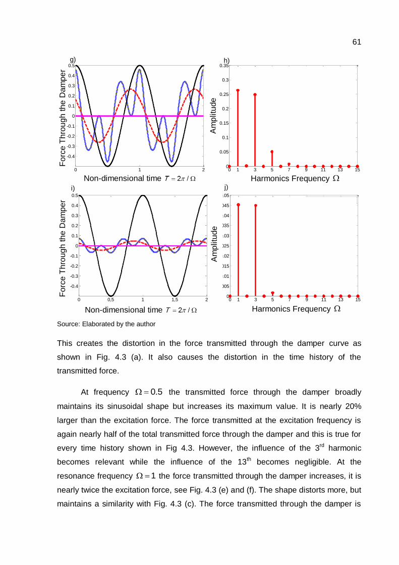
61

0 1 3 5 7 9 11 13 150

0.005

0.01

0.015

0.02

0.025

0.03

0.035

0.04

0.045

0.05

DC value - At Zero

0 1 3 5 7 9 11 13 150

0.05

0.1

0.15

0.2

0.25

0.3

0.35

DC value - At Zero

0 1 2

-0.4

-0.3

-0.2

-0.1

0

0.1

0.2

0.3

0.4

0.5

Harmonics Frequency

Am

plitu

de

Non-dimensional time

Fo

rce

Th

rou

gh

th

e D

am

pe

r g) h)

Harmonics Frequency

0 0,5 1 1,5 2

-0.4

-0.3

-0.2

-0.1

0

0.1

0.2

0.3

0.4

0.5

Am

plitu

de

Fo

rce

Th

rou

gh

th

e D

am

pe

r

i)

Non-dimensional time

j)

Source: Elaborated by the author

This creates the distortion in the force transmitted through the damper curve as

shown in Fig. 4.3 (a). It also causes the distortion in the time history of the

transmitted force.

At frequency 0 5. the transmitted force through the damper broadly

maintains its sinusoidal shape but increases its maximum value. It is nearly 20%

larger than the excitation force. The force transmitted at the excitation frequency is

again nearly half of the total transmitted force through the damper and this is true for

every time history shown in Fig 4.3. However, the influence of the 3rd harmonic

becomes relevant while the influence of the 13th becomes negligible. At the

resonance frequency 1 the force transmitted through the damper increases, it is

nearly twice the excitation force, see Fig. 4.3 (e) and (f). The shape distorts more, but

maintains a similarity with Fig. 4.3 (c). The force transmitted through the damper is

62

mainly composed of the 1st, the 3rd, the 5th, and the 7th harmonic, and the rest of the

harmonics are negligible.

At 1 5. the force transmitted through the damper is just a little smaller than the

amplitude of the excitation force, see Fig 4.3 (g). From Fig 4.3 (h) can be seen that

the force through the damper is mainly composed if the 1st and the 3rd harmonic and

in lesser extend of the 5th harmonic.

In the isolation region at 2 the force transmitted through the damper

reduces considerably, see Figs 4.3 (i) and (j). It is nearly 15% of the amplitude of the

excitation force and consists of the fundamental and the 3rd harmonic. Comparing the

force transmitted through the spring (Figs 4.2 (i)) and the force transmitted through

the damper (Figs 4.3 (i)) at this frequency it can be seen that the force through the

damper is nearly one quarter of the force transmitted through the spring. This is

consistent with the findings in Chapter 3 where it was found that at this frequency the

transmitted force is mainly dominated by the force trough the spring.

Comparing Figs. 4.2 and 4.3 it can be seen that specifically for the large value

use here to the amplitude of the excitation force, the force transmitted through the

damper exceeds the amplitude of the excitation force, while the force transmitted

through the spring do not do it, whatever the excitation frequency. This is because

the large amplitude of the excitation force produces large mass displacements and it

makes considerably increase the force through the damper while the force through

the spring increases but in a lesser extent. It also can be seen that the distortion in

the time history curves of the transmitted force of Fig. 4.1 are due to the force

transmitted through the damper, as would be expected, and not to the force through

the spring.

4.3.4 Nonlinear Damping Coefficient

The expression of the viscous damping force is the multiplication of two

parameters: the damping coefficient which is constant for a linear damper and the

relative velocity. For the damper considered in this work the damping coefficient is a

63

Figure 4.4 - Time histories for the non-dimensional damping coefficient function fc of the nonlinear

damper and its frequency spectrum when h

10 and e

0 5ˆ .F for a) 0 3. , c) 0 5. , e) 1 ,

g) 1 5. , i) 2 . Blue solid line – time history the nonlinear damping coefficient fc , yellow dotted

line – Fourier series of the time history, red dashed line – second harmonic of the Fourier series,

magenta horizontal line – mean value (DC level) of the signal. b), d), f), h) and j) – Frequency

spectrum with the DC value at zero and the first fifteen harmonics from the Fourier series of the time

history for nonlinear damping coefficient curves shown in a), c), e), g) and j).

0 2 4 6 8 10 12 14 150

0.5

1

1.5

2

2.5

DC value - At Zero

Harmonics Frequency 0 0,5 1 1,5 2

0

0.5

1

1.5

2

2.5

3

3.5

4

Da

mp

ing

Co

effic

ien

t F

un

ctio

n

Non-dimensional time

Am

plitu

de

a) b)

0 2 4 6 8 10 12 14 150

0.5

1

1.5

2

2.5

3

DC value - At Zero

0 0.5 1 1,5 20

0.5

1

1.5

2

2.5

3

3.5

4

d)

Da

mp

ing

Co

effic

ien

t F

un

ctio

n

Am

plitu

de

c)

Non-dimensional time

0 2 4 6 8 10 12 14 150

0.5

1

1.5

2

2.5

DC value - At Zero

0 0,5 1 1,5 20

0.5

1

1.5

2

2.5

3

3.5

Da

mp

ing

Co

effic

ien

t F

un

ctio

n

Am

plitu

de

f) e)

Harmonics Frequency

Non-dimensional time Harmonics Frequency

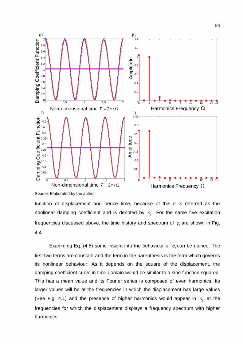
64

Source: Elaborated by the author

function of displacement and hence time, because of this it is referred as the

nonlinear damping coefficient and is denoted by fc . For the same five excitation

frequencies discussed above, the time history and spectrum of fc are shown in Fig.

4.4.

Examining Eq. (4.5) some insight into the behaviour of fc can be gained. The

first two terms are constant and the term in the parenthesis is the term which governs

its nonlinear behaviour. As it depends on the square of the displacement, the

damping coefficient curve in time domain would be similar to a sine function squared.

This has a mean value and its Fourier series is composed of even harmonics. Its

larger values will be at the frequencies in which the displacement has large values

(See Fig. 4.1) and the presence of higher harmonics would appear in fc at the

frequencies for which the displacement displays a frequency spectrum with higher

harmonics.

0 0,5 1 1,5 20

0.05

0.1

0.15

0.2

0.25

0.3

0.35

0.4

0.45

0.5

0 2 4 6 8 10 12 14 150

0.2

0.4

0.6

0.8

1

1.2

1.4

DC value - At Zero

0 0,5 1 1,5 20

0.2

0.4

0.6

0.8

1

1.2

1.4

1.6

1.8

2D

am

pin

g C

oe

ffic

ien

t F

un

ctio

n

Am

plitu

de

g) h)

Non-dimensional time Harmonics Frequency

Da

mp

ing

Co

effic

ien

t F

un

ctio

n i)

0 2 4 6 8 10 12 14 150

0.05

0.1

0.15

0.2

0.25

0.3

0.35

DC value - At Zero

Non-dimensional time Harmonics Frequency

j)

Am

plitu

de

65

The higher displacements for the nonlinear system are at frequencies less than or

equal to the resonance frequency, so the higher values for fc are at the frequencies

0 3. , 0 5. and 1 . This can be seen in Figs. 4.4 (a), (c) and (e) which

show the time histories of fc for these excitation frequencies. There is a small

influence of harmonics higher than the 2nd in the time histories which can be seen

clearly in the frequency spectra shown in Figs. 4.4 (b), (d) and (f). Some influence of

the 4th harmonic for 1 , and the 4th and the 6th harmonic for 0 5. and 1

can be seen. For frequencies higher the resonance frequencies, 1 5. and 2

there is a negligible influence of higher harmonics. Only the mean value and the 2nd

harmonic are necessary to reconstruct the original signals for the nonlinear damping

coefficient, this is shown in Figs. 4.4 (g) and (h) for 1 5. and Figs. 4.4 (i) and (j)

for 2 . At these frequencies the amplitude of fc starts to reduce, with its

amplitude being less than one.

Although the results depend on the parameters used in the beginning of the

chapter, which are the same used in Chapter 3, in general it can be concluded that

the nonlinear damping coefficient at frequencies inside the resonance region

produces the effect of increasing the amplitude of the velocity; as its maximum values

are larger than one. On the other hand for frequencies in the isolation region, the

nonlinear damping coefficient produces the opposite effect, reducing the amplitude of

the velocity; as its maximum values are smaller than one. This is a different effect

compared with that of a viscous coefficient damping which is constant whatever the

frequency value.

4.3.5 Velocity of the mass

In determining the causes of the unfavourable behaviour of the transmitted

force shown in Fig. 3.8, the transmitted force has been decomposed into forces

transmitted through the spring and through the damper. The nonlinear force

transmitted through the damper can be studied by examining the nonlinear damping

coefficient and the velocity of the mass. In this subsection the time history and the

66

Figure 4.5 - Time histories for the non-dimensional mass velocity of the nonlinear damper and its

frequency spectrum when h

10 and e

0 5ˆ .F for a) 0 3. , c) 0 5. , e) 1 , g) 1 5. , i)

2 . Blue solid line – time history for the mass velocity, yellow dotted line – Fourier series of the time

history, red dashed line – first harmonic of the Fourier series, magenta horizontal line – mean value

(DC level) of the signal. b), d), f), h) and j) – Frequency spectrum with the DC value at zero and the

first fifteen harmonics from the Fourier series of the time history for nonlinear damping coefficient

curves shown in a), c), e), g) and j).

0 1 3 5 7 9 11 13 150

0.02

0.04

0.06

0.08

0.1

0.12

0.14

0.16

DC value - At Zero

0 0,5 1 1,5 2

-0.3

-0.2

-0.1

0

0.1

0.2

0.3

Harmonics Frequency

Ve

locity

Non-dimensional time

Am

plitu

de

a) b)

0 1 3 5 7 9 11 13 150

0.05

0.1

0.15

0.2

0.25

0.3

0.35

DC value - At Zero

0 0,5 1 1,5 2-0.5

-0.4

-0.3

-0.2

-0.1

0

0.1

0.2

0.3

0.4

0.5

0 1 3 5 7 9 11 13 150

0.05

0.1

0.15

0.2

0.25

0.3

0.35

0.4

0.45

0.5

DC value - At Zero

0 0,5 1 1,5 2

-0.6

-0.4

-0.2

0

0.2

0.4

0.6

f)

Harmonics Frequency Non-dimensional time

Non-dimensional time Harmonics Frequency

Ve

locity

Am

plitu

de

Ve

locity

Am

plitu

de

e)

c) d)

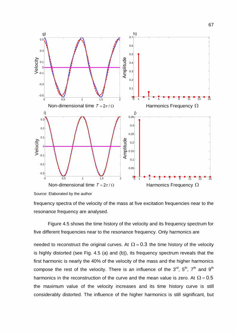
67

0 1 3 5 7 9 11 13 150

0.1

0.2

0.3

0.4

0.5

0.6

0.7

DC value - At Zero

Harmonics Frequency

0 0,5 1 1,5 2

-0.5

-0.3

-0.1

0

0.1

0.3

0.5

Non-dimensional time

Am

plitu

de

g) h)

0 0,5 1 1,5 2

-0.3

-0.2

-0.1

0

0.1

0.2

0.3

i)

0 1 3 5 7 9 11 13 150

0.05

0.1

0.15

0.2

0.25

0.3

0.35

DC value - At Zero

j)

Ve

locity

Am

plitu

de

Ve

locity

Non-dimensional time Harmonics Frequency

Source: Elaborated by the author

frequency spectra of the velocity of the mass at five excitation frequencies near to the

resonance frequency are analysed.

Figure 4.5 shows the time history of the velocity and its frequency spectrum for

five different frequencies near to the resonance frequency. Only harmonics are

needed to reconstruct the original curves. At 0 3. the time history of the velocity

is highly distorted (see Fig. 4.5 (a) and (b)), its frequency spectrum reveals that the

first harmonic is nearly the 40% of the velocity of the mass and the higher harmonics

compose the rest of the velocity. There is an influence of the 3rd, 5th, 7th and 9th

harmonics in the reconstruction of the curve and the mean value is zero. At 0 5.

the maximum value of the velocity increases and its time history curve is still

considerably distorted. The influence of the higher harmonics is still significant, but

68

only up to the 7th harmonic. Because of this the shape of the curve is very similar to

the time history for 0 3. . This is illustrated in Figs. 4.5 (c) and (d).

At the resonance frequency, 1 , the maximum value increases but there is

the influence of mainly two frequencies; the fundamental frequency and three times

this frequency and there is a very slight influence of the 5th harmonic. This is

illustrated in

Figures. 4.5 (e) and (f). An important issue is that at frequencies lower than

the resonance frequency the nonlinearity in the velocity is very pronounced; In Figs.

4.5 (b) and (d) can be seen the considerable presence of higher harmonics in the

amplitude spectrum of the velocity of the mass at 0 3. and 0 5. , respectively.

The presentence of these higher harmonics with considerable amplitude in the

velocity of the mass are due to the high-pass filter effect caused by calculating the

velocity from displacement response which possess higher order harmonics as

shown in Figs. 4.2 (b) and (d) where the amplitude of the higher order harmonics is

small. When the velocity is calculated from such a displacement response, the higher

harmonics increases its amplitudes. For instance consider a displacement signal

represented in time domain by

1 1

3 52 3

sin sin sinu t t t t (4.6)

where is the an angular frequency and t is time. If u t is differentiated in order to

obtain velocity it leads to

3 5

3 52 3

cos cos cosu t t t t (4.7)

It can be seen the effect of differentiating a signal composed by several

harmonics, it increases the amplitude of the higher harmonics and maintains the

amplitude at the fundamental frequency, just as a high-pass filter.

At frequencies higher than the resonance frequency, the velocity amplitude

decreases, at 1 5. the velocity is mainly composed of the fundamental frequency

and has a slightly influence of the 3rd harmonic, it is illustrated in Figs. 4.5 (g) and (h).

In the isolation region, at 2 , there is just the velocity at the fundamental

69

frequency, evidently because at these frequencies the displacement response is very

small (see Figs. 4.5 (i) and (j)).

4.4 Conclusions

In this chapter the reasons why the transmitted force to the base becomes

distorted at frequencies close to the resonance region has been investigated.

Studying the time history and the spectra of the transmitted force it was found that its

high values at the resonance frequency region are produced by the presence of

higher harmonics in the transmitted force curves besides the force at the excitation

frequency. These high harmonics are markedly presents in the force transmitted

through the damper instead of the force transmitted through the spring.

Studying the force through the spring it was found that, specifically for the

large amplitude value of the excitation force used here, the maximum force

transmitted through it, is close to the amplitude of the excitation force and regardless

the excitation frequency it is not larger than the excitation force but at frequencies

higher than the resonance frequency the force transmitted through the spring starts

to decreases. From the study of the force transmitted through the damper there was

found that at frequencies near to the resonance frequency its amplitude exceeds the

amplitude of the excitation force.

It was found that for the nonlinear damping force the damping coefficient is

amplitude and hence time dependent which is very different compared by a viscous

damping coefficient which is constant. It is a nonlinear function whose maximum

values are more than one for frequencies below the resonance frequency and less

than one for frequencies above the resonance region. That is because the

dependence of the nonlinear coefficient on the mass displacement; which at the

resonance region is large while at the isolation region is very small.

It was also found that the velocity is the most important cause of the

nonlinearity in the damping force because of the presence of high harmonics in its

time histories when excited with frequencies corresponding to the resonance

frequency region. The presence of high harmonics with considerable amplitudes in

the velocity curves is caused by the effect of increasing them when the displacement

signal is differentiated which is similar to the effect of a high-pass filter.

It can also be concluded that the nonlinearity of the damping force could be

seen as the multiplication of two nonlinearities coming from the nonlinear damping

coefficient which increases the amplitude of the harmonics of the velocity of the

mass.

70

5 CONCLUSIONS

5.1 Summary of the Dissertation

This Chapter summarizes the work done in this dissertation and presents the

main conclusions obtained as well as the recommendations for further work. The

principal goals in this dissertation were to compare the performance between the a

linear and a nonlinear vibration isolation system with its damper orientated at ninety

degrees with respect to the spring and to analyse the time histories of the transmitted

force at frequencies close to the resonance frequency. To achieve these objectives

the dissertation was divided as follows:

Chapter 1 introduced the topic of vibration isolation and to present a review of

the literature in this area in the specific context of nonlinear vibration isolation.

In Chapter 2 the characteristics of a SDOF linear isolation system when its

mass is excited by a harmonic force and when the system is harmonically excited by

the base have been reviewed. The equation describing the system in both cases has

been obtained to define force and displacement transmissibility for a SDOF isolation

system. The way in which the system parameters affect the isolations systems at

different frequency regions has been investigated and a discussion about the

concepts of transient, steady state and resonance frequency has been presented.

In Chapter 3 the characteristics of a SDOF nonlinear isolation system in which

the damper is orientated at ninety degrees to the spring was investigated. Its

performance was compared with that of a SDOF isolation system by comparing their

force and displacement transmissibilities in the cases in which the systems were

excited by a harmonic force and by a harmonic base excitation. A study was

undertaken in which low excitation amplitudes were considered. In this case, the

nonlinear damping force was approximated to an equivalent viscous damping force.

A numerical analysis was conducted for high amplitude excitation.

The force transmissibility for high amplitude excitation levels from Chapter 3

had undesirable performance at frequencies close to the resonance frequency. In

71

Chapter 4 the time histories for the force transmitted to the base at different

frequencies near the resonance frequency and their frequency spectra have been

studied. The time histories for the force transmitted through the spring and the force

transmitted through the damper together with their spectra have also been studied.

Finally, the force transmitted through the damper has been separated into a time

dependent damping coefficient and the velocity of the mass to gain some insight into

the nonlinear effects.

5.2 Main Conclusions

It has been shown that the force produced by a damper orientated at ninety

degrees with respect to the spring can be approximated to an equivalent viscous

damping force. It has also been shown that for low amplitude excitation the damping

force depends on the square of the relative displacement and it makes the nonlinear

isolator suitable for vibration isolation for low levels of excitation.

Analytical expressions have been derived which describe the dynamic

behaviour and the performance of the nonlinear isolator for low amplitude excitation.

From these it can be concluded that at low amplitude excitation:

- The force and displacement transmissibility at the resonance frequency are

smaller than for the linear system provided that e

250ˆ /h

F and

ˆ /F 3

e h4 for the force excited system and h

34ˆ /Y and

ˆ /Y h

250 for the base excited system.

- At high frequencies for the force excited system, the nonlinear system

performs better than the linear isolator, behaving as if it were undamped.

Regarding the displacement transmissibility, the nonlinear system also

performs better than the linear system at the resonance frequency but there is

a detrimental effect at high frequencies.

For high excitation amplitudes and from the numerical results it has been

shown that:

72

- Regarding the force transmissibility, the nonlinear system at the resonance

frequency performs better than the linear system but there is an undesirable

effect at frequencies close to the resonance frequency which makes larger the

force transmissibility compared with that of the linear system. At high

frequencies the nonlinear system performs very well, behaving as if it were

undamped. This is one of the important results of this dissertation.

- Regarding the displacement transmissibility close to the resonance frequency,

the nonlinear isolator preforms better than the linear isolator but at high

frequencies its performance is worse than the linear system.

From the analysis of the time histories and the Fourier series of the

transmitted force for the nonlinear system it has been found that the high values

close to the resonance frequency are due to the presence of higher harmonics.

Decomposing the transmitted force at frequencies close to the resonance region it

has been shown that specifically for the large amplitude of the excitation force use in

this work; the amplitude of the force transmitted through the spring is not larger than

the amplitude of the excitation force. However, this is not the case with the force

transmitted through the damper.

Decomposing the force through the nonlinear damper it has been shown that

the damping coefficient is not constant but varies with time and is a nonlinear

function. It causes an increase in the amplitude of the velocity of the mass at

frequencies greater than the resonance frequency and decreases the amplitude of

the velocity in the isolation region. It has also been shown that the velocity of the

mass is the most important cause of the nonlinear behaviour of the damping force.

Finally, it can be concluded that the nonlinearity of the damping force arises from the

geometry of the system.

5.3 Recommendation for Further Work

In this work the damper was oriented so that it is at ninety degrees from the

spring. Further work can investigate the performance of SDOF isolation systems with

different positions of the damper with respect to the spring between 0 and ninety

degrees.

Another possibility is to investigate the performance of a SDOF isolation

system with two linear springs; one of which is at ninety degrees from the other and

73

is parallel to a linear viscous damper, the external disturbance is applied at ninety

degrees to the damper.

The performance of a similar system to that investigated in this work could be

studied but considering two degrees of freedom so that the mass can move in the

plane formed by the damper axis and the spring axis.

74

REFERENCES

FULLER, C. R., ELLIOT, S. J., NELSON, P. A. Active control of vibration. 1. ed.

London: Academic Press Limited, 1996. HARRIS, C. M., CREDE, C. E.. Shock and vibration hanbook. 5. ed. Washington: McGraw Hill Inc, 1961. LAALEJ, H. et al. Application of non-linear damping to vibration isolation: an experimental study. Nonlinear Dynamics, Dordrech, v. 69, n. 69, p. 409-421, 2012. LANG, Z. Q. et al.Theoretical study of the effects of nonlinear viscous damping on vibration isolation of sdof systems. Journal of Sound and Vibration, London, v.

323, n. 1-2, p. 352-365, 2009. MILOVANOVIC, Z.; KOVACIC, I.; BRENNAN M. J. On the Displacement Transmissibility of a base excited viscously damped nonlinear vibration isolator. Journal of Vibration and Acoustics, New York, v. 131, n. 054502, p. 1-7, 2009. RAO, S. S. Vibrações mecânicas. 4. ed. Americana: Pearson Education, 2008. RAVINDRA, B., MALLIK, A. K. Performance of non-linear vibration isolators under harmonic excitation. Journal of Sound and Vibration, London, v. 170, n. 3, p. 325-

337, 1994. RIVIN, E. I. Passive vibration isolation. 1. ed. New York: ASME Press, 2003. RUZICKA J. E.; DERBY, T. F. Influence of damping in vibration isolation. 1 ed. Washington: The Shock And Vibration Information Center: Naval Research Laboratory, 1971. SHIN, K.; HAMMOND, J. K. Fundamentals of signal processing for sound and vibration engineers. 1. ed. London: John Wiley & Sons Ltd, 2008.

SNOWDON, J. C. Vibration isolation: use and characterization. Journal of the Acoustical Society of America, New York, v. 66, n. 5, p. 1245-1274, 1979. STEIDEL JÚNIOR, R. F. J. An Introduction to mechanical vibration. 3. ed. Washington: John Wiley & Sons, 1989. TANG, B.; BRENNAN M, J. A Comparison of two nonlinear damping mechanism in a vibration isolator. Journal of Sound and Vibration, London, v. 332, n. 3, p. 510-520, 2013. TANG, B.; BRENNAN; J. M. A comparison of the effects of nonlinear damping on the free vibration of a single-degree-of-freedom system. Journal of Vibration and Acoustics, New York, v. 134, n. 024501, p. 1-5, 2012.

75

THOMSON, W. T., DAHLEH, M. D. Theory of vibration with application. 5. ed.

New Jersey: Prentice Hall, 1996. YAN B. Active vibration isolation with a distributed parameter isolator. 2007. 250 f. Thesis (PhD in Mechanical Engineering) - University of Southampton, Faculty of Engineering, Science and Mathematics, Institute of Sound and Vibration Research, Southampton, 2007.