Comparing the Correlative Holdridge Model to Mechanistic Biogeographical Models for Assessing Vegetation Distribution Response to Climatic Change

COMPARING THE CORRELATIVE HOLDRIDGE MODEL TOMECHANISTIC BIOGEOGRAPHICAL MODELS FOR ASSESSING

VEGETATION DISTRIBUTION RESPONSE TO CLIMATIC CHANGE

DAVID N. YATES1,2, TIMOTHY G. F. KITTEL1,3 and REGINA FIGGE CANNON1

1National Center for Atmospheric Research, Boulder, CO 80307, U.S.A.2Department of Civil Engineering, University of Colorado, Boulder, CO 80203, U.S.A.

3Natural Resource Ecology Laboratory, Colorado State University, Ft. Collins, CO 80523, U.S.A.

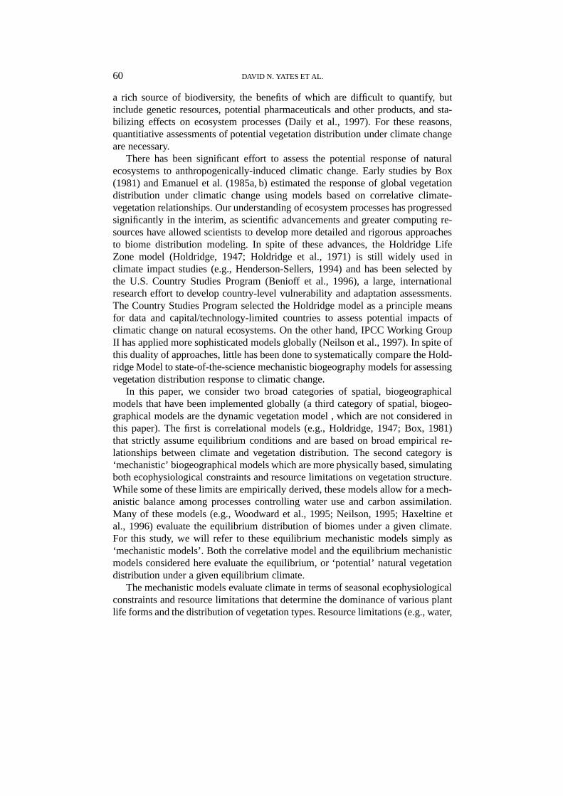
Abstract. A well-established and widely used correlative climate-vegetation model (Holdridge LifeZone model) was compared to three mechanistic simulation models (BIOME2, Dynamic GlobalPhytogeography Model (DOLY), and Mapped Atmosphere-Plant-Soil System (MAPSS)) for theconterminous United States under contemporary climate and a set of future climates prescribed bythree Global Circulation Model experiments. Output from the mechanistic models were from the Ve-getation/Ecosystem Modeling and Analysis Project (VEMAP) intercomparison. Holdridge modelingapproaches, using a ‘Simple’ implementation (vegetation distribution based on biotemperature andprecipitation alone) or a ‘Full’ implementation (vegetation distribution based on biotemperature, pre-cipitation, altitudinal region, latitudinal belt, and transitional vegetation zones), represented currentpotential natural U.S. vegetation poor to fair, respectively. The more sophisticated mechanistic mod-els were superior at reproducing potential vegetation under current climate compared to Holdridge,although there was significant variability among these models. The Holdridge implementations gen-erally showed similar or greater climate sensitivity with respect to spatial redistribution of vegetationcompared to the mechanistic models run both with and without doubled CO2 levels; however, thesensitivity of the Holdridge model depended on the implementation. Reduced sensitivity of the mech-anistic models arises from direct (physiological) CO2 effects and other compensating feedbacks notcaptured by the Holdridge model. The greater degree of physical realism in the mechanistic modelsmakes them the model class of choice for climate impact assessment. However, under circumstancesof limited data availability, computation resources, and access to mechanistic models and modelexpertise, simple correlational models such as Holdridge may be the only method that can be applied.The paper makes some recommendations on the use of the Holdridge model for impact assessmentif it is the only available model.

1. Introduction

Regional climate is likely to exhibit a range of spatially complex responses toanthropogenically-induced climate variations, affecting both the function and spa-tial distribution of terrestrial ecosystems (VEMAP Members, 1995; Kattenburget al., 1997; Cramer et al., 1998; Pan et al., 1998). These ecosystems representa substantial resource base for socio-economic development and also represent

Climatic Change44: 59–87, 2000.© 2000Kluwer Academic Publishers. Printed in the Netherlands.

60 DAVID N. YATES ET AL.

a rich source of biodiversity, the benefits of which are difficult to quantify, butinclude genetic resources, potential pharmaceuticals and other products, and sta-bilizing effects on ecosystem processes (Daily et al., 1997). For these reasons,quantitiative assessments of potential vegetation distribution under climate changeare necessary.

There has been significant effort to assess the potential response of naturalecosystems to anthropogenically-induced climatic change. Early studies by Box(1981) and Emanuel et al. (1985a, b) estimated the response of global vegetationdistribution under climatic change using models based on correlative climate-vegetation relationships. Our understanding of ecosystem processes has progressedsignificantly in the interim, as scientific advancements and greater computing re-sources have allowed scientists to develop more detailed and rigorous approachesto biome distribution modeling. In spite of these advances, the Holdridge LifeZone model (Holdridge, 1947; Holdridge et al., 1971) is still widely used inclimate impact studies (e.g., Henderson-Sellers, 1994) and has been selected bythe U.S. Country Studies Program (Benioff et al., 1996), a large, internationalresearch effort to develop country-level vulnerability and adaptation assessments.The Country Studies Program selected the Holdridge model as a principle meansfor data and capital/technology-limited countries to assess potential impacts ofclimatic change on natural ecosystems. On the other hand, IPCC Working GroupII has applied more sophisticated models globally (Neilson et al., 1997). In spite ofthis duality of approaches, little has been done to systematically compare the Hold-ridge Model to state-of-the-science mechanistic biogeography models for assessingvegetation distribution response to climatic change.

In this paper, we consider two broad categories of spatial, biogeographicalmodels that have been implemented globally (a third category of spatial, biogeo-graphical models are the dynamic vegetation model , which are not considered inthis paper). The first is correlational models (e.g., Holdridge, 1947; Box, 1981)that strictly assume equilibrium conditions and are based on broad empirical re-lationships between climate and vegetation distribution. The second category is‘mechanistic’ biogeographical models which are more physically based, simulatingboth ecophysiological constraints and resource limitations on vegetation structure.While some of these limits are empirically derived, these models allow for a mech-anistic balance among processes controlling water use and carbon assimilation.Many of these models (e.g., Woodward et al., 1995; Neilson, 1995; Haxeltine etal., 1996) evaluate the equilibrium distribution of biomes under a given climate.For this study, we will refer to these equilibrium mechanistic models simply as‘mechanistic models’. Both the correlative model and the equilibrium mechanisticmodels considered here evaluate the equilibrium, or ‘potential’ natural vegetationdistribution under a given equilibrium climate.

The mechanistic models evaluate climate in terms of seasonal ecophysiologicalconstraints and resource limitations that determine the dominance of various plantlife forms and the distribution of vegetation types. Resource limitations (e.g., water,

COMPARING THE CORRELATIVE HOLDRIDGE MODEL 61

light, nutrients) determine major structural characteristics of vegetation, includ-ing leaf area and the presence of woody vegetation. Ecophysiological constraints,based on bioclimatic variables including growing degree-days and minimum wintertemperatures, then determine the other characteristics of vegetation such as thetype of woody vegetation (e.g., needleleaf vs. broadleaf). The models account forwater resource limitation on plant growth (each model often applying a differentapproach) through soil moisture availability based on water budget calculationsincluding computations of potential and actual evapotranspiration and runoff.

The correlative models, on the other hand, are essentially climate classifierswhich commonly relate mean climate to the observed, large-scale distributionof vegetation (e.g., Smith et al., 1992). The shortcomings of correlative modelsinclude their empirical approach to climate-vegetation relationships, often inad-equate representation of important seasonal variability, and subjective approachesto biome classification. However, because of their practicality and universal ac-cessibility, these simpler models continue to be used for assessing the potentialresponse of vegetation to climate perturbations (e.g., Prentice, 1990; Smith et al.,1992; Henderson-Sellers, 1994; Benioff et al., 1996; Lugo et al., 1998). The Hold-ridge Life Zone model (Holdridge, 1947; Holdridge et al., 1971), which relatesannual average precipitation and temperature to specific vegetation types, has per-haps been the most widely used correlative model for assessing biome response toclimate change.

In this study, we examined differences in vegetation distribution generated bytwo implementations of the correlative Holdridge model and three equilibriummechanistic models (BIOME2, Dynamic Global Phytogeography Model (DOLY),and Mapped Atmosphere-Plant-Soil-System (MAPSS)). We compared these mod-els in terms of biases in control runs for the conterminous United States undercontemporary climate and CO2 conditions and in terms of their sensitivity toaltered forcing with runs under doubled atmospheric CO2 concentrations coupledwith a range of climate scenarios. Results for the three mechanistic models werefrom the Vegetation/Ecosystem Modeling and Analysis Project (VEMAP) Phase 1intercomparison (VEMAP Members 1995) and are available on the world wideweb (URL= http://www.cgd.ucar.edu/vemap). From the comparison between cor-relative and mechanistic models, we make recommendations to policy makersregarding the appropriateness of these and related models for studies of ecologicalvulnerability to climatic change.

62D

AVID

N.YA

TE

SE

TA

L.

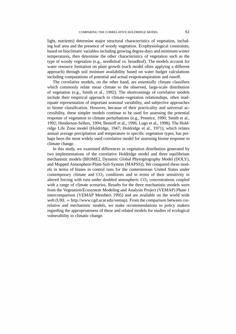
Figure 1. The Holdridge Life Zone Model, showing the aggregation of the 13 SiVVEG classes mapped to the 38 Life Zones according to the SimpleHoldridge Implementation (SHI).


2. Approach

2.1. IMPLEMENTATION OF THE HOLDRIDGE MODEL

The Holdridge model relates the large-scale distribution of vegetation to two keyclimate variables, average annual precipitation (specified as the annual total) andannual average biotemperature, to define ecological climate zones or ‘Life Zones’.Average biotemperature is the average temperature, derived from monthly meantemperatures in our case, over a year with contributing values set to 0◦C forthose below 0◦C. The model uses a third variable, the ratio of annual potentialevapotranspiration to precipitation, which is a function of the other two variables(biotemperature and precipitation) and, therefore, is not a required input for thelife-zone classification scheme. Each zone is depicted by a hexagon formed byintersecting intervals defined by the three climate variables plotted along logar-ithmic axes of a triangular coordinate system (see Figure 1). The Holdridge modeldivides vegetation into over 100 broad Life Zones according to the set of hexagonsidentified along the biotemperature, precipitation, and potential evapotranspirationto precipitation ratio axes and additionally distinguished by altitudinal belt andlatitudinal region. In addition, Holdridge recognized transitional Life Zones inthe corners of the hexagons (see Figure 1), which leads to a more finely dividedclimate/life zone space of over 600 uniquely identifiable regions.

The model is based on annual climate, with no explicit measure of seasonality.However, Holdridge et al. (1971) modified this model in an attempt to accountfor differences in seasonal variability between the equatorial region and the sub-tropics (between 12◦ and 25◦ latitude). At higher latitudes in this region, thereis a wider range of mean monthly temperatures during the year and, during thewarmer months, periods of sustained heat negatively affect plant growth more thanwithin the equatorial region. As a result, Holdridge revised his calculation of meanbiotemperature by assigning a value of 0◦C for all unit-period (in our case monthlymean) temperatures above 30◦C, as well as less than 0◦C. The model has noprovision for altered vegetation-climate relationships under elevated CO2 arisingfrom direct physiological effects.

The Holdridge model has been applied in different ways to assess the impacts ofclimate change on vegetation/ecosystem distributions (Henderson-Sellers, 1994).This is primarily due to differences in assigning or aggregating Holdridge’s LifeZones to more commonly recognized biome or vegetation classes used on global orregional maps. In some cases, the more complex hexagonal Life Zone boundarieswere followed (solid lines in Figure 1, Section 2.1), while others simply followedthe precipitation and biotemperature axes (horizontal and right-tending verticaldashed lines in Figure 1, Section 2.1). Furthermore, aggregation of the Life Zonesinto broader vegetation types has differed, and alternative naming conventions havebeen used to identify Life Zones (e.g., ‘prairie’ has been assigned to Holdridge’smoist forest and ‘savanna’ to dry forest). In some applications with aggregated life


zones, climate boundaries were tuned to more closely match observed vegetationdistributions (e.g., Ciret, 1997).

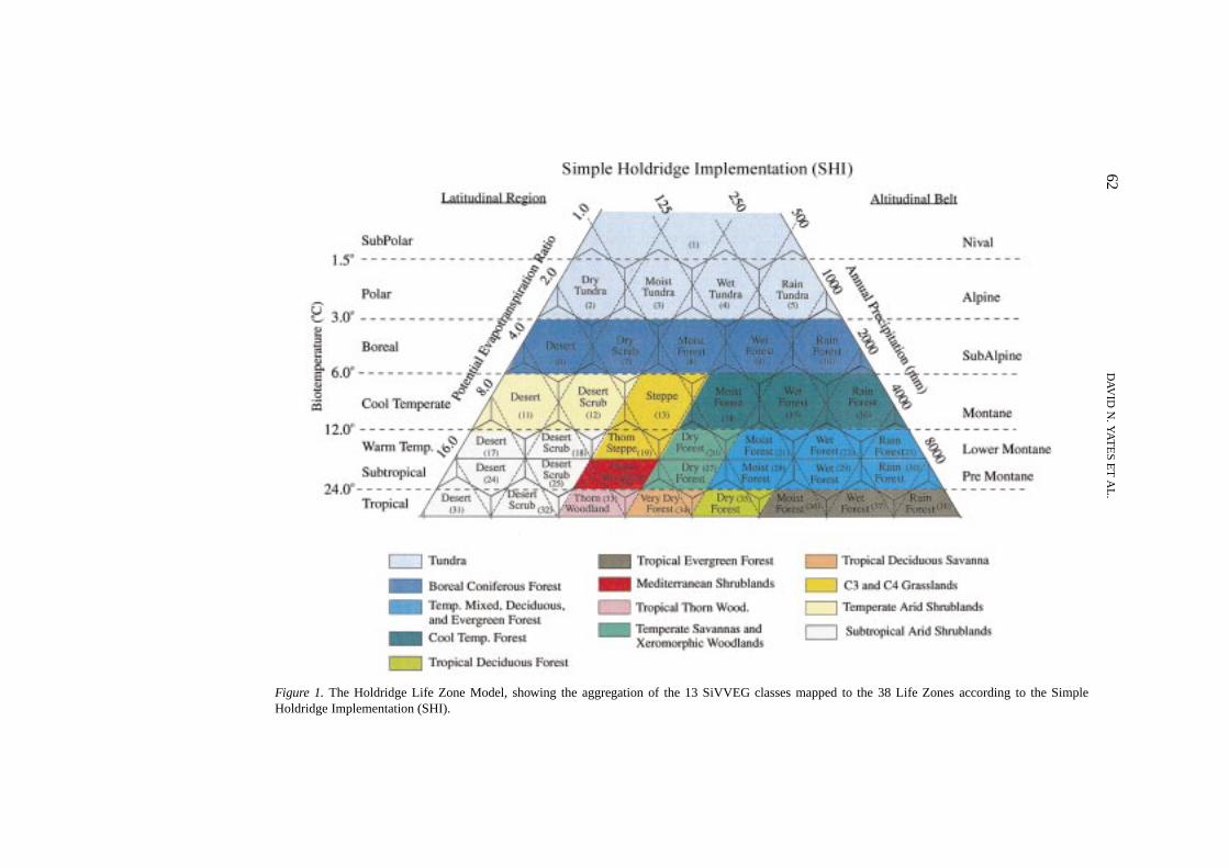
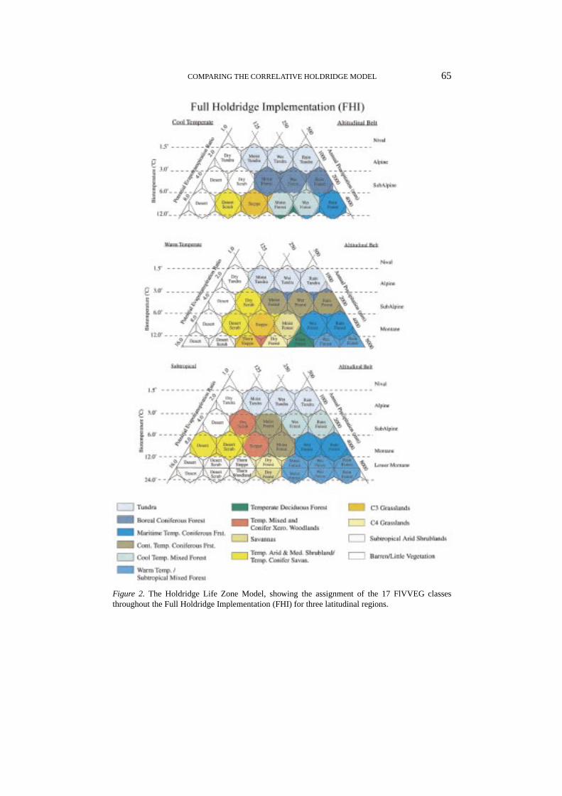
Given these differences in the application of the Holdridge model, we choseto evaluate it according to two different approaches. In both implementations,we aggregated Holdridge’s Life Zone into broader vegetation categories to matchthose used by the mechanistic models in VEMAP. However, the implementationsdiffered by the complexity with which we divided the Holdridge climate space. Inthe first, labeled Simple Holdridge Implementation (SHI), we discriminated broadvegetation types identified only by biotemperature and precipitation axes, formingtrapezoidal biome boundaries (Figure 1). In the second, labeled Full HoldridgeImplementation (FHI), we more finely divided the climate space, closely followingthe original model description set forth in Holdridge (1947) and Holdridge et al.(1971). In the FHI, we divided the climate space by the hexagonal boundaries,adjacent transitional zones, and both altitudinal and latitudinal extent (Figure 2).We present the aggregation of the life zones and the assignment of these broadertypes to the Holdridge climate space for these two implementations in Section 2.5.

2.2. MECHANISTIC MODELS AND VEMAP EXPERIMENTS

VEMAP Members (1995) compared vegetation distribution simulated by threemechanistic models, BIOME2 (Haxeltine et al., 1996), DOLY (Woodward andSmith, 1994; Woodward et al., 1995), and MAPSS (Neilson, 1995) under variousclimate change and CO2 conditions. The models differ in their approach to mod-eling ecophysiological constraints and resource limitations using different formsof coupled carbon and water flux algorithms. The models also differ in climatevariable input requirements depending on their representation of physiological andwater budget processes, and they all include the influence of CO2 concentrations onplant physiology, though it is modeled differently by the three models (see VEMAPMembers, 1995). The relative importance of direct CO2 effects on the models’vegetation distribution response was evaluated by VEMAP Members (1995). Thereader is referred to VEMAP Members (1995) and corresponding model referencesfor complete descriptions of the mechanistic models.

In VEMAP Phase 1, the three mechanistic models were driven by present-dayclimatology or by altered climate forced by doubled-CO2 scenarios (from three cli-mate models, Section 2.4) and by 1× or 2× atmospheric CO2 concentrations (355or 710 ppm CO2, respectively). For this study, we compared biases of the modelsby evaluating ‘control runs’ of the two Holdridge model implementations undercurrent climate and control runs of the mechanistic models (under contemporaryclimate and 1× CO2 levels). To evaluate model sensitivities to altered forcing,we compared Holdridge altered climate runs to mechanistic model runs with bothaltered climate (2× CO2 induced) and altered climate and doubled atmosphericCO2 levels (2×CO2). The latter runs, with 2×CO2 climate and 2×CO2 concen-trations, were analyzed for the mechanistic models because together the climate


Figure 2. The Holdridge Life Zone Model, showing the assignment of the 17 FlVVEG classesthroughout the Full Holdridge Implementation (FHI) for three latitudinal regions.


and CO2 changes constitute a consistent scenario. However, because direct CO2

effects are not considered in the Holdridge model, we compared the Holdridgemodel climate sensitivity to those of the mechanistic models under 1×CO2 levelsas well.

2.3. VEMAP CLIMATE DATA

Comparison of the correlative and mechanistic models required the use of a com-mon input dataset, which was developed for the VEMAP model comparison (Kittelet al., 1995, 1996; see also VEMAP web site, URL= http://www.cgd.ucar.edu/vemap). This dataset consists of 0.5◦ × 0.5◦ latitude/longitude gridded long-termmean climate, soil, potential natural vegetation data, and climate scenarios forthe conterminous U.S. Climate variables include: characteristic daily and monthlymean minimum and maximum surface air temperatures, precipitation, total in-cident solar radiation, surface air humidity, and near-surface wind speed. Thisstandardized database maintained (1) temporal consistency (daily and monthlyclimate sets had the same monthly values), (2) spatial consistency (influences oftopography were accounted for), and (3) physical consistency (relationships amongclimate variables and among soil properties were maintained). The monthly versionof the climate data was used in VEMAP to run MAPSS and BIOME2, and thedaily version for DOLY. We used mean monthly temperature and precipitation datafields from this dataset to derive annual mean biotemperature and mean annualprecipitation for both implementations of the Holdridge model.

2.4. CLIMATE CHANGE SCENARIOS

The three climate scenarios used in VEMAP were from the Geophysical FluidDynamics Laboratory (GFDL; R30 2.22◦ × 3.75◦ grid run; Manabe and Wetherald,1990; Wetherald and Manabe, 1990), Oregon State University (OSU; Schlesingerand Zhao, 1989), and United Kingdom Meteorological Office (UKMO; Wilsonand Mitchell, 1987). The scenarios were based on three atmospheric general circu-lation model (GCM) equilibrium climate sensitivity experiments for a double-CO2

atmosphere. These models included a simple ‘mixed-layer’ ocean representationwhich includes heat storage and the vertical exchange of heat and moisture withthe atmosphere but omits dynamically determined horizontal ocean heat transport.It is recognized that these represent an older class of GCM experiments, however,regionally-averaged sensitivities of the models are similar to those of more recentcoupled ocean-atmosphere GCMs (Kittel et al., 1998).

These three scenarios represent a range of climate sensitivity over the UnitedStates, with OSU having the lowest temperature and precipitation sensitivity (+3◦Cand 4% increase, respectively, on an annual basis), UKMO with the highest temper-ature sensitivity and mid-range precipitation sensitivity (6.7◦C and 12% increase,respectively), and GFDL-R30 representing a mid-range temperature sensitivity


and highest precipitation sensitivity (4.3◦C and 21% increase, respectively). Re-gional precipitation changes varied widely among models and with season, withthe UKMO showing increased annual precipitation throughout most of the U.S.,except for decreases in south-central and southeastern regions. OSU showed in-creased annual precipitation in the north-west central region and along the easternseaboard and decreases in most of the southern and southwestern U.S. GFDL-R30showed decreased precipitation in the Central Great Plains and the southeast andlarger increases in Texas and the southwest (see VEMAP Members, 1995 or website for details).

2.5. VEGETATION CLASSIFICATION SCHEMES

To evaluate the models’ simulated distribution of vegetation under current condi-tions (control runs), we used a potential natural vegetation map (VVEG) developedby VEMAP to describe the potential, present-day vegetation of the conterminousUnited States (Kittel et al., 1995, 1996). Distribution of these types was basedon a gridded map of Küchler’s (1964, 1975) potential natural vegetation. For thepurposes of VEMAP and this intercomparison, this distribution was assumed tobe in equilibrium with current climate. Vegetation classes were aggregated fromKüchler’s map and were defined in terms of dominant life-form and leaf character-istics and, in the case of grasslands, physiologically with respect to the dominanceof species with a C3 versus C4 photosynthetic pathway.

For comparison of VEMAP model output with that of the Holdridge model,the original 21 VVEG classes were combined according to the two different ag-gregation schemes: one for comparison with the Simple Holdridge Implementation(SHI) consisting of 13 vegetation classes (SiVVEG; Table I) and a second forcomparison with the Full Holdridge Implementation (FHI) containing 17 classes(FlVVEG; Section 2.5.2). Less aggregation was required for FHI than SHI becausethe climate space is more finely divided in the former. Details of the model-ing methodology used for the SHI and FHI can be found in the accompanyingappendix.

2.6. ASSESSMENT CRITERIA

We compared the Holdridge model and the mechanistic models in terms of (1)model biases, comparing control runs to the distribution of potential vegetationunder current conditions (SiVVEG and FlVVEG, Figure 3), and (2) model climatesensitivity, comparing altered-forcing runs with corresponding controls. To com-pare the different runs, we used the kappa statistic (k), a measure of map agreement,where a value of 1.0 indicates complete agreement.

Landis and Koch (1977) gave qualitative ranks to the kappa statistic, withvalues from 0.7 to 1.0 indicating very good-to-perfect agreement, 0.55 to 0.70good-to-very good agreement, 0.40 to 0.55 fair-to-good agreement, 0.2 to 0.4 poor-to-fair agreement, and 0.0 to 0.2 no-to-poor agreement. Because we compared the


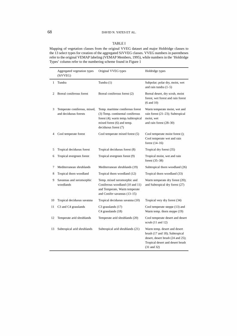
TABLE I

Mapping of vegetation classes from the original VVEG dataset and major Holdridge classes tothe 13 select types for creation of the aggregated SiVVEG classes. VVEG numbers in parenthesesrefer to the original VEMAP labeling (VEMAP Members, 1995), while numbers in the ‘HoldridgeTypes’ column refer to the numbering scheme found in Figure 1

Aggregated vegetation types Original VVEG types Holdridge types

(SiVVEG)

1 Tundra Tundra (1) Subpolar; polar dry, moist, wet

and rain tundra (1–5)

2 Boreal coniferous forest Boreal coniferous forest (2) Boreal desert, dry scrub, moist

forest, wet forest and rain forest

(6 and 10)

3 Temperate coniferous, mixed, Temp. maritime coniferous forest Warm temperate moist, wet and

and deciduous forests (3) Temp. continental coniferous rain forest (21–23); Subtropical

forest (4); warm temp./subtropical moist, wet

mixed forest (6) and temp. and rain forest (28–30)

deciduous forest (7)

4 Cool temperate forest Cool temperate mixed forest (5) Cool temperate moist forest ();

Cool temperate wet and rain

forest (14–16)

5 Tropical deciduous forest Tropical deciduous forest (8) Tropical dry forest (35)

6 Tropical evergreen forest Tropical evergreen forest (9) Tropical moist, wet and rain

forest (35–38)

7 Mediterranean shrublands Mediterranean shrublands (19) Subtropical thorn woodland (26)

8 Tropical thorn woodland Tropical thorn woodland (12) Tropical thorn woodland (33)

9 Savannas and xeromorphic Temp. mixed xeromorphic and Warm temperate dry forest (20);

woodlands Coniferous woodland (10 and 11) and Subtropical dry forest (27)

and Temperate, Warm temperate

and Conifer savannas (13–15)

10 Tropical deciduous savanna Tropical deciduous savanna (10) Tropical very dry forest (34)

11 C3 and C4 grasslands C3 grasslands (17) Cool temperate steppe (13) and

C4 grasslands (18) Warm temp. thorn steppe (19)

12 Temperate arid shrublands Temperate arid shrublands (20) Cool temperate desert and desert

scrub (11 and 12)

13 Subtropical arid shrublands Subtropical arid shrublands (21) Warm temp. desert and desert

brush (17 and 18); Subtropical

desert, desert brush (24 and 25);

Tropical desert and desert brush

(31 and 32)

CO

MP

AR

ING

TH

EC

OR

RE

LAT

IVE

HO

LDR

IDG

EM

OD

EL

69Figure 3.Potential vegetation distribution of the conterminous United States based on the VEMAP vegetation classification for the two aggregation schemes,labeled SiVVEG and FlVVEG.


Holdridge model (SHI and FHI) using two different aggregations of the VVEGdataset (SiVVEG and FlVVEG), two sets of kappa values were generated for eachcomparison to the mechanistic models. The kappa statistic reflects both spatialshifts (redistribution) and total area changes of individual biomes (Monserud andLeemans, 1992). We separately evaluated map changes in terms of net change inarea of major biome categories (i.e., forests, grasslands, shrublands, and savannas).

3. Results and Discussion

3.1. COMPARING HOLDRIDGE AND MECHANISTIC MODELS UNDER

CONTEMPORARY CLIMATE

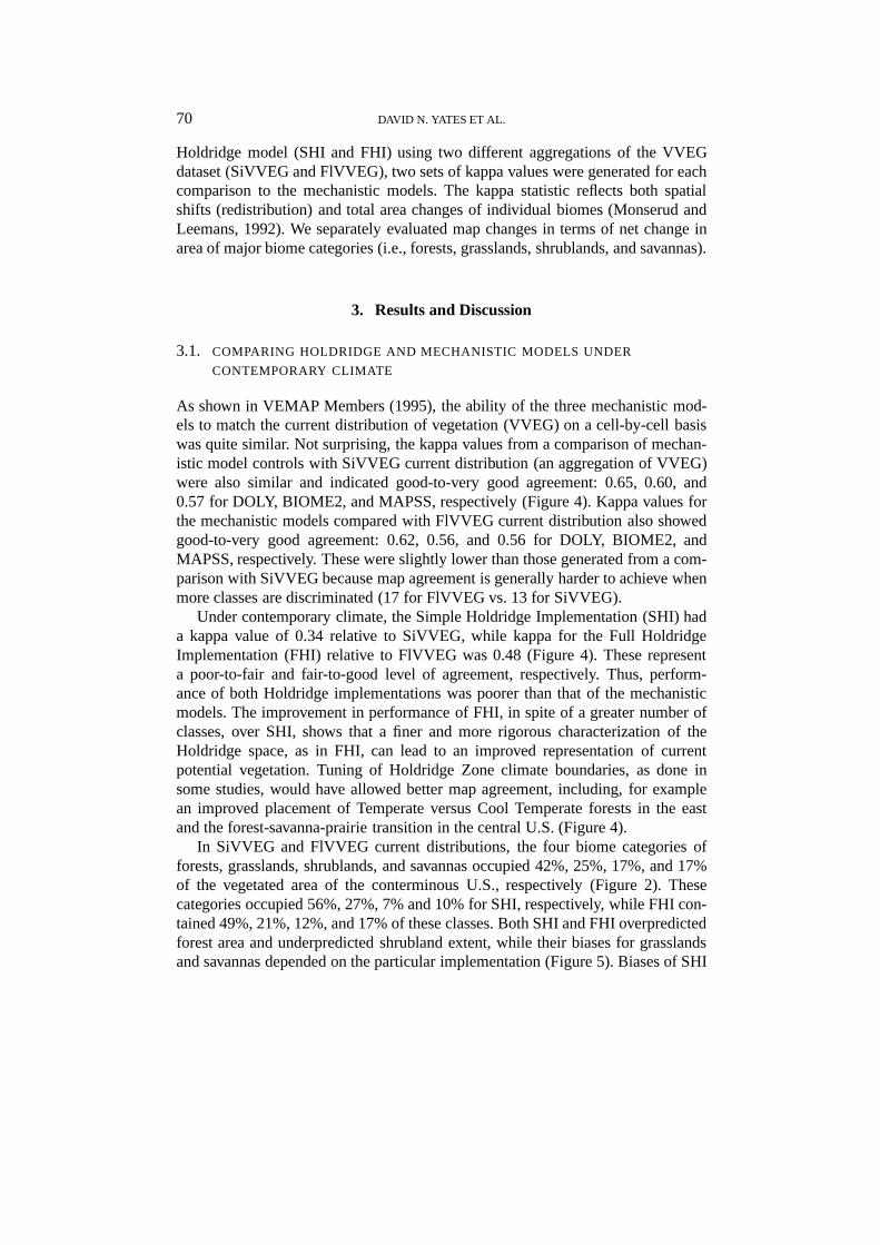
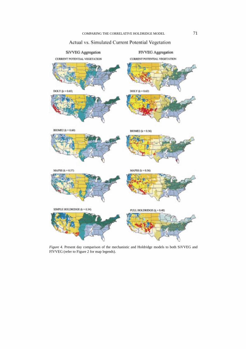
As shown in VEMAP Members (1995), the ability of the three mechanistic mod-els to match the current distribution of vegetation (VVEG) on a cell-by-cell basiswas quite similar. Not surprising, the kappa values from a comparison of mechan-istic model controls with SiVVEG current distribution (an aggregation of VVEG)were also similar and indicated good-to-very good agreement: 0.65, 0.60, and0.57 for DOLY, BIOME2, and MAPSS, respectively (Figure 4). Kappa values forthe mechanistic models compared with FlVVEG current distribution also showedgood-to-very good agreement: 0.62, 0.56, and 0.56 for DOLY, BIOME2, andMAPSS, respectively. These were slightly lower than those generated from a com-parison with SiVVEG because map agreement is generally harder to achieve whenmore classes are discriminated (17 for FlVVEG vs. 13 for SiVVEG).

Under contemporary climate, the Simple Holdridge Implementation (SHI) hada kappa value of 0.34 relative to SiVVEG, while kappa for the Full HoldridgeImplementation (FHI) relative to FlVVEG was 0.48 (Figure 4). These representa poor-to-fair and fair-to-good level of agreement, respectively. Thus, perform-ance of both Holdridge implementations was poorer than that of the mechanisticmodels. The improvement in performance of FHI, in spite of a greater number ofclasses, over SHI, shows that a finer and more rigorous characterization of theHoldridge space, as in FHI, can lead to an improved representation of currentpotential vegetation. Tuning of Holdridge Zone climate boundaries, as done insome studies, would have allowed better map agreement, including, for examplean improved placement of Temperate versus Cool Temperate forests in the eastand the forest-savanna-prairie transition in the central U.S. (Figure 4).

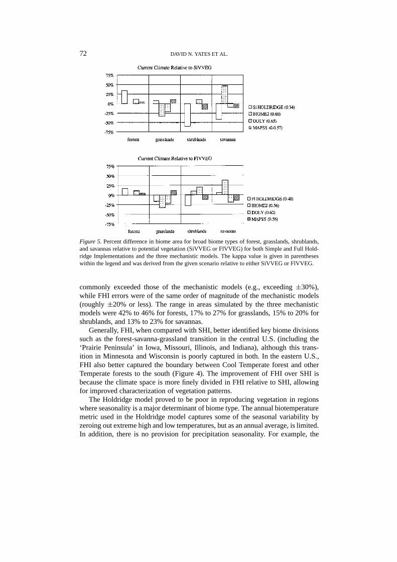
In SiVVEG and FlVVEG current distributions, the four biome categories offorests, grasslands, shrublands, and savannas occupied 42%, 25%, 17%, and 17%of the vegetated area of the conterminous U.S., respectively (Figure 2). Thesecategories occupied 56%, 27%, 7% and 10% for SHI, respectively, while FHI con-tained 49%, 21%, 12%, and 17% of these classes. Both SHI and FHI overpredictedforest area and underpredicted shrubland extent, while their biases for grasslandsand savannas depended on the particular implementation (Figure 5). Biases of SHI


Figure 4. Present day comparison of the mechanistic and Holdridge models to both SiVVEG andFlVVEG (refer to Figure 2 for map legends).


Figure 5.Percent difference in biome area for broad biome types of forest, grasslands, shrublands,and savannas relative to potential vegetation (SiVVEG or FlVVEG) for both Simple and Full Hold-ridge Implementations and the three mechanistic models. The kappa value is given in parentheseswithin the legend and was derived from the given scenario relative to either SiVVEG or FlVVEG.

commonly exceeded those of the mechanistic models (e.g., exceeding±30%),while FHI errors were of the same order of magnitude of the mechanistic models(roughly±20% or less). The range in areas simulated by the three mechanisticmodels were 42% to 46% for forests, 17% to 27% for grasslands, 15% to 20% forshrublands, and 13% to 23% for savannas.

Generally, FHI, when compared with SHI, better identified key biome divisionssuch as the forest-savanna-grassland transition in the central U.S. (including the‘Prairie Peninsula’ in Iowa, Missouri, Illinois, and Indiana), although this trans-ition in Minnesota and Wisconsin is poorly captured in both. In the eastern U.S.,FHI also better captured the boundary between Cool Temperate forest and otherTemperate forests to the south (Figure 4). The improvement of FHI over SHI isbecause the climate space is more finely divided in FHI relative to SHI, allowingfor improved characterization of vegetation patterns.

The Holdridge model proved to be poor in reproducing vegetation in regionswhere seasonality is a major determinant of biome type. The annual biotemperaturemetric used in the Holdridge model captures some of the seasonal variability byzeroing out extreme high and low temperatures, but as an annual average, is limited.In addition, there is no provision for precipitation seasonality. For example, the


temperate arid shrubland (northern Nevada, eastern Oregon, and southern Idaho) isa region that the Holdridge model did not reproduce well. Most often, SHI and FHIindicated this region as grasslands (C3 grasses in FHI). This part of the temperatearid shrublands is a shrub-steppe ecotone, a transition zone from core shrublandsto core C3 grasslands. The temperate arid shrubland region has similar annualprecipitation and biotemperature as the C3 grassland zone, but is characterized bylower summer precipitation which favors shrublands over grasslands. The Hold-ridge model is not capable of identifying this seasonal effect, and therefore assignsthese cells as C3 grasslands.

Compared to the Holdridge model, the three mechanistic models were superiorat locating forest-grassland and grassland-shrubland transition zones, although theydiffered amongst themselves in their placement of specific biome boundaries suchas between C3 and C4 grasslands, and the savanna ecotone separating the cent-ral grasslands and eastern forests. Each mechanistic model differs in its approachto approximating the C3/C4 and forest/grassland transitions, but these models in-clude seasonality effects via thermal rules and calculations of water budgets whichgenerally improved their ability to place vegetation transition zones.

3.2. COMPARING HOLDRIDGE AND MECHANISTIC MODELS UNDER CLIMATIC

CHANGE

VEMAP Members (1995) showed that the mechanistic models were sensitive toaltered climate under the three climate scenarios and under both 1× and 2× CO2

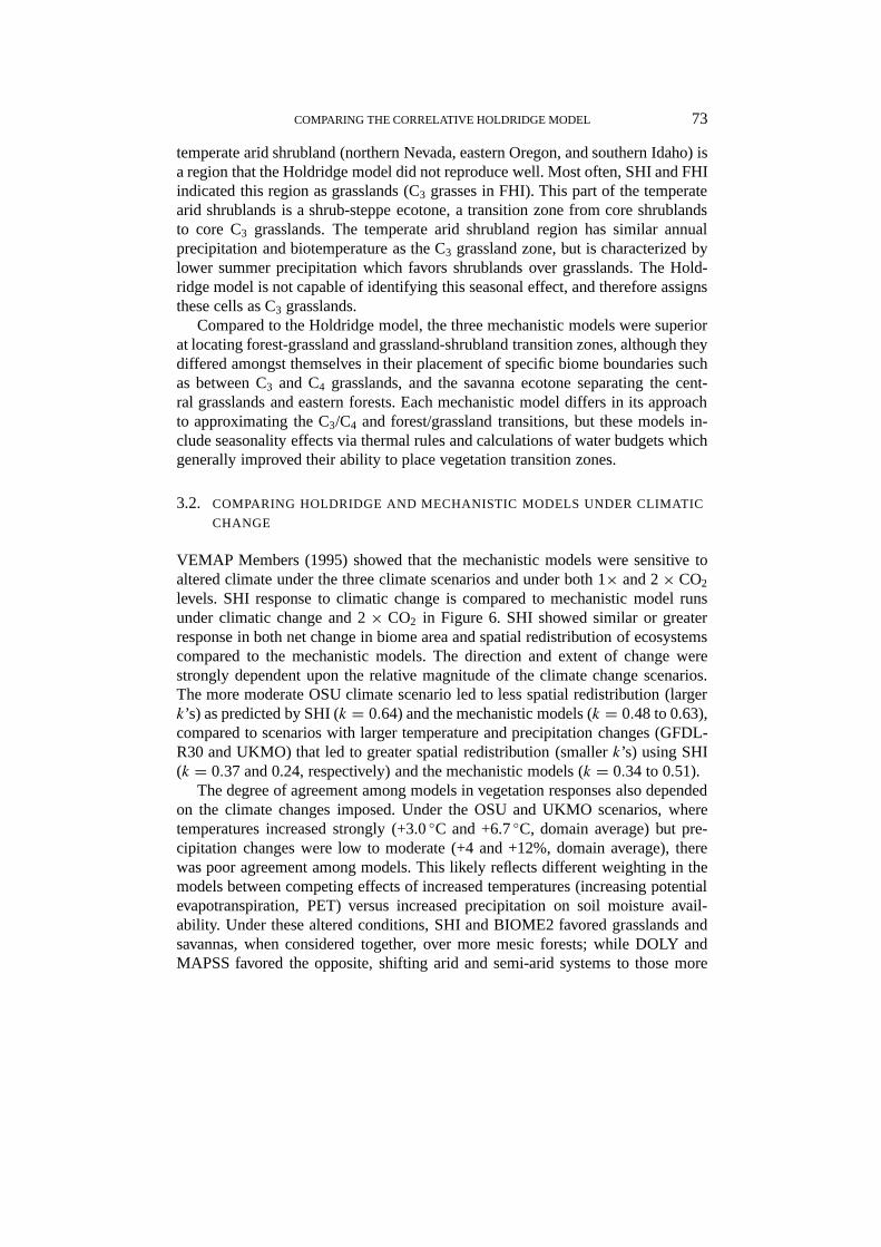
levels. SHI response to climatic change is compared to mechanistic model runsunder climatic change and 2× CO2 in Figure 6. SHI showed similar or greaterresponse in both net change in biome area and spatial redistribution of ecosystemscompared to the mechanistic models. The direction and extent of change werestrongly dependent upon the relative magnitude of the climate change scenarios.The more moderate OSU climate scenario led to less spatial redistribution (largerk’s) as predicted by SHI (k = 0.64) and the mechanistic models (k = 0.48 to 0.63),compared to scenarios with larger temperature and precipitation changes (GFDL-R30 and UKMO) that led to greater spatial redistribution (smallerk’s) using SHI(k = 0.37 and 0.24, respectively) and the mechanistic models (k = 0.34 to 0.51).

The degree of agreement among models in vegetation responses also dependedon the climate changes imposed. Under the OSU and UKMO scenarios, wheretemperatures increased strongly (+3.0◦C and +6.7◦C, domain average) but pre-cipitation changes were low to moderate (+4 and +12%, domain average), therewas poor agreement among models. This likely reflects different weighting in themodels between competing effects of increased temperatures (increasing potentialevapotranspiration, PET) versus increased precipitation on soil moisture avail-ability. Under these altered conditions, SHI and BIOME2 favored grasslands andsavannas, when considered together, over more mesic forests; while DOLY andMAPSS favored the opposite, shifting arid and semi-arid systems to those more


Figure 6. Percent change in biome area for broad biome types of forest, grasslands, shrublands,and savannas for Simple Holdridge Implementation and mechanistic models compared against eachmodels’ SiVVEG control. The value in parentheses within the legend is the kappa value (k), under(a) OSU, (b) GFDL-R30, and (c) UKMO climate change scenarios derived from the given scenariorelative to the modeled prediction of potential vegetation given contemporary climate and 1× CO2.

mesic (shrublands to grasslands, and shrublands and grasslands to savannas andforests (Figure 6a, c).

On the other hand, under the GFDL-R30 scenario, with the largest domain-averaged precipitation increase (+21%) and intermediate temperature changes(+4.3◦C), SHI and the mechanistic models consistently showed a net transitionfrom grasslands and shrublands to forests and savannas (Figure 6b). Here, whereclimate change was dominated by the increase in precipitation, that reduced the


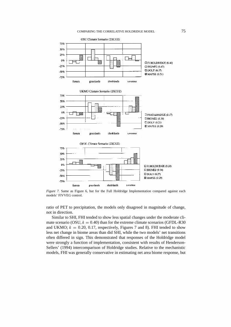
Figure 7. Same as Figure 6, but for the Full Holdridge Implementation compared against eachmodels’ FlVVEG control.

ratio of PET to precipitation, the models only disagreed in magnitude of change,not in direction.

Similar to SHI, FHI tended to show less spatial changes under the moderate cli-mate scenario (OSU,k = 0.40) than for the extreme climate scenarios (GFDL-R30and UKMO;k = 0.20, 0.17, respectively, Figures 7 and 8). FHI tended to showless net change in biome areas than did SHI, while the two models’ net transitionsoften differed in sign. This demonstrated that responses of the Holdridge modelwere strongly a function of implementation, consistent with results of Henderson-Sellers’ (1994) intercomparison of Holdridge studies. Relative to the mechanisticmodels, FHI was generally conservative in estimating net area biome response, but


Figure 8a.

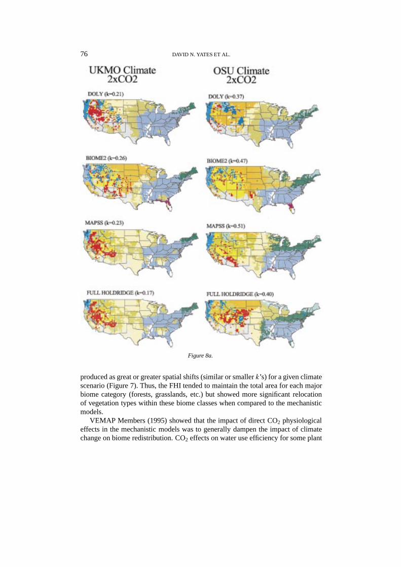
produced as great or greater spatial shifts (similar or smallerk’s) for a given climatescenario (Figure 7). Thus, the FHI tended to maintain the total area for each majorbiome category (forests, grasslands, etc.) but showed more significant relocationof vegetation types within these biome classes when compared to the mechanisticmodels.

VEMAP Members (1995) showed that the impact of direct CO2 physiologicaleffects in the mechanistic models was to generally dampen the impact of climatechange on biome redistribution. CO2 effects on water use efficiency for some plant


Figure 8b.

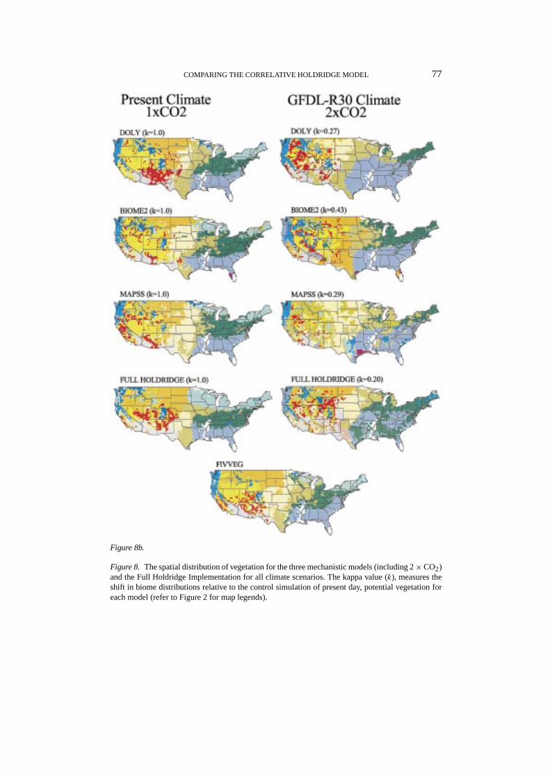
Figure 8. The spatial distribution of vegetation for the three mechanistic models (including 2×CO2)and the Full Holdridge Implementation for all climate scenarios. The kappa value (k), measures theshift in biome distributions relative to the control simulation of present day, potential vegetation foreach model (refer to Figure 2 for map legends).


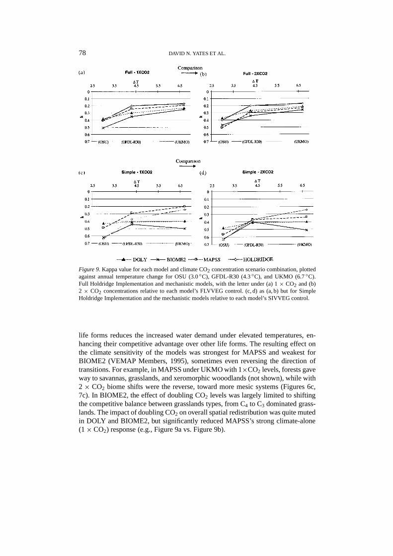
Figure 9.Kappa value for each model and climate CO2 concentration scenario combination, plottedagainst annual temperature change for OSU (3.0◦C), GFDL-R30 (4.3◦C), and UKMO (6.7◦C).Full Holdridge Implementation and mechanistic models, with the letter under (a) 1× CO2 and (b)2 × CO2 concentrations relative to each model’s FLVVEG control. (c, d) as (a, b) but for SimpleHoldridge Implementation and the mechanistic models relative to each model’s SIVVEG control.

life forms reduces the increased water demand under elevated temperatures, en-hancing their competitive advantage over other life forms. The resulting effect onthe climate sensitivity of the models was strongest for MAPSS and weakest forBIOME2 (VEMAP Members, 1995), sometimes even reversing the direction oftransitions. For example, in MAPSS under UKMO with 1×CO2 levels, forests gaveway to savannas, grasslands, and xeromorphic wooodlands (not shown), while with2× CO2 biome shifts were the reverse, toward more mesic systems (Figures 6c,7c). In BIOME2, the effect of doubling CO2 levels was largely limited to shiftingthe competitive balance between grasslands types, from C4 to C3 dominated grass-lands. The impact of doubling CO2 on overall spatial redistribution was quite mutedin DOLY and BIOME2, but significantly reduced MAPSS’s strong climate-alone(1× CO2) response (e.g., Figure 9a vs. Figure 9b).


4. Conclusions and Recommendations

Four broad conclusions were drawn regarding the use of the Holdridge model forassessing vegetation distribution response to climatic change. Firstly, the mechan-istic models were superior to the correlative Holdridge model (both Simple and FullImplementations) in simulating potential vegetation under current climate condi-tions, suggesting that the additional details present in the mechanistic models isbeneficial as compared with a simpler correlative model like Holdridge (Bonan,1993; Bugmann and Martin, 1995). Secondly, the Simple Holdridge Implementa-tion (SHI) performed more poorly than the Full Holdridge Implementation (FHI)at simulating current potential vegetation. These two results reflect the limitationsof the Holdridge system due to possibly/probably the lack of mechanistic interac-tions and limited representation of the role of seasonality (which together resultin strict climate boundaries in terms of annual climate) and difficulties in match-ing/aggregating commonly recognized vegetation classes into the Holdridge LifeZones. FHI reduced some aggregation problems due to increased flexibility derivedby identifying latitudinal zones, altitudinal belts, and transition regions.

Thirdly, FHI showed greater sensitivity to altered climate forcing than themechanistic models in terms of the magnitude of the spatial redistribution of ve-getation types. FHI was more sensitive under the more extreme climate scenarios.This greater sensitivity relative to the mechanistic models was partly the result ofcompensating direct CO2 effects (i.e., ameliorating increased water stress underelevated temperatures) in the mechanistic models. However, large uncertaintiesin the nature of direct CO2 effects on ecosystems over long periods remain. Thesensitivity of the mechanistic models to direct CO2 effects could be due to aninappropriate understanding, and hence modeling, of CO2 mechanisms in plants.

Finally, SHI showed greater sensitivity under larger magnitude climate changescenarios relative to FHI and the mechanistic models in terms of net area changeof major biome types. However, under the smaller magnitude climate change, SHIshowed responses smaller or similar in magnitude to those of FHI and the mechan-istic models. In addition, differences between FHI and SHI sensitivities were suchthat, under certain climate change scenarios, biome changes were in the oppositedirection. These differences were, however, similar in nature to those found amongthe mechanistic models.

These conclusions resulted in the following observations and recommenda-tions for use of models for assessing the potential impacts of climate change onvegetation redistribution:

Model Choice.The Holdridge implementations generally showed similar orgreater climate sensitivity with respect to spatial redistribution of vegetation com-pared to the mechanistic models run both with and without doubled CO2 levels(e.g., Figures 9c, d). Reduced sensitivity of the mechanistic models arises fromCO2 effects, other compensating feedbacks (e.g., between leaf area productionand water balance), and potentially compensating changes in climate inputs to the


mechanistic models (e.g., higher vapor pressures under higher temperatures) thatare not considered in the Holdridge model. These effects tend to maintain or moreconservatively shift the distribution of vegetation zones in the mechanistic models.On the other hand, allowance in the mechanistic models for changes in the seasonaldistribution of climate (e.g., timing of precipitation) and for compounding changesin multiple climate impacts (e.g., lower vapor pressure with higher temperatures)has the potential for enhancing the sensitivity of the mechanistic models over theHoldridge model. These uncoupled features of the mechanistic models work toblur the climatic boundaries of vegetation zones that are defined in terms of strictlimits of annual mean temperature and precipitation in the Holdridge scheme. Infact, the climate/vegetation relationships of the Holdridge model reflect multipleeffects. For example, climate change scenarios with alterations in sunshine hours,atmospheric thickness, radiation, etc., would lump into a single temperature effectso that neither compounding nor canceling effects would occur.

The explicit incorporation of ecophysical processes and resource constraintsalong with multivariate and seasonal representation of climate space gives themechanistic models a high degree of physical realism missing in the Holdridgemodel. This provides a scientific basis for exercising the mechanistic models un-der novel environmental conditions outside the realm for which the Holdridgemodel was developed (e.g., under higher CO2 concentrations, new combinationsof daylength and temperature, and other weather and climate factors). However,the mechanistic models are quite complex and have many tuning parameters thatcould lead to offsetting errors if biophysical processes, that are not completelyunderstood, are not modeled correctly. These errors could lead to an unrealisticresponse to new climate conditions. This possibility is supported by the divergingbehavior of the three mechanistic models that were analyzed in this study.

In spite of these concerns, the greater degree of physical realism in the mechan-istic models makes them the model class of choice for climate impact assessment.This is especially the case given greater availability of global data sets (Neilsonet al., 1997; Cramer et al., 1998; New et al., 1998), improved access to PC-basedversions of the mechanistic models (e.g., albeit an older version of BIOME; Pren-tice et al., 1992) and more recent advances in mechanistic models that include thedevelopment of Dynamic Global Vegetation Models (DGVMs) and their couplingwith biogeochemistry models (Neilson and Running, 1996; Daly et al., 1998).These model improvements incorporate time-dependent ecological responses (e.g.,vegetation dieback, migration, succession, and soil development) to transient for-cings including climate trends and inter-annual variability, atmospheric CO2 levels,nitrogen deposition, and disturbance. Suites of these models are currently beingaddressed by Phase 2 of VEMAP (see Kittel et al., 1998) and the IBGP PotsdamDGVM intercomparison (Cramer et al., 1998).

Options for the Holdridge Model.Under circumstances of limited access tomechanistic models and modeling expertise and limited availability of high res-olution, multivariate regional data sets and computation resources, simple and


more readily available models may be the only methods that can be applied forclimate impact studies. This includes correlative models such as Holdridge, whichare based on simple relationships between aggregate measures of climate andvegetation.

With respect to the Holdridge model, our results suggest that there may be a pre-ferred way to implement this scheme. There was more convergence in equilibriumresponse to climate change among the mechanistic and Holdridge models under theFull Holdridge vegetation aggregation. This arose because the finer aggregationincluded important vegetation distinctions that are sensitive to climate (e.g., C3

versus C4 dominated grasslands, xeromorphic woodlands versus savannas). Re-moving some of these distinctions in the SHI aggregation reduced the sensitivity ofthe models in different ways (e.g., Figure 9a, b). The finer aggregation also allowedFHI to better capture the climatic extent of key transition zones (e.g., for savan-nas). Given this convergence with FHI, we recommend, with the caveats notedbelow, the following course for implementing the Holdridge model. Specifically,one should first account for latitudinal region and altitudinal belt. Secondly, theidentification of life and transition zones should be carefully considered duringthe initial process of aggregating the Holdridge biome space to vegetation typesselected for a particular study. Transitional vegetation zones, such as savannasand shrub-steppes, are likely the most sensitive to small changes in climate butare also the most likely biomes to be misrepresented or omitted by the Holdridgemodel due to the strict and/or broad climate ranges assigned to the life zones andthe role of seasonality in controlling their distribution. While a major departurefrom Holdridge’s original scheme, tuning of Life Zone climate boundaries wouldalso improve representativenesss of aggregated zones and performance of modelsimulated vegetation under current conditions.

BIOME (Prentice et al., 1992) is a mechanistic model with limited data andcomputation requirements, which incorporates mechanistic feedbacks and seasonalinputs, though omits direct CO2 effects. This model requires, in addition to tem-perature and precipitation, monthly mean percent sunshine hours and soil textureinformation (available globally at 0.5◦ resolution; e.g., Leemans and Cramer, 1991;FAO, 1974). However, deficiencies in the simpler models, including Holdridge,point to the clear and urgent need for the vegetation modeling community toprovide, particularly for developing countries, off-the-shelf, state-of-the-sciencemodels as tools for resource agencies charged with developing vulnerability andadaptation assessments.

Nonetheless, the following caveats apply to the use of the Holdridge model inimpact studies: (1) the climate sensitivity of the Holdridge model is dependenton implementation, and (2) many important mechanisms that control vegetationresponse (e.g., seasonality, direct CO2 effects, etc.) are not captured by the model’scorrelations with annual temperature and precipitation. Additionally, as for allequilibrium models, transient responses of ecosystems may differ strongly (e.g., in


sign) from estimated equilibrium responses due to non-linear interactions amongprocesses with different response times.

Uncertainties and Policy Development.Regardless of model choice, applicationof biogeographical models in assessment studies needs to be in consideration ofassociated uncertainties. These are demonstrated by the range of model responsesand arise from model formulation and inadequacies in our understanding of keyecological processes (VEMAP Members, 1995). Henderson-Sellers (1994) notesthat uncertainties in emission scenarios, climate models, impact models, and thepolicy formation process are likely reasons for limited policy development and im-plementation with respect to greenhouse gas reduction. If scientists are to generatecredible studies that will guide policy makers, an overall evaluation of a systemsvulnerability in light of current scientific uncertainties in ecosystem response toclimate change and elevated CO2 must be properly communicated. As greenhousegas reduction polices are developed, they will rely on models such as those presen-ted here. However, it is unlikely or at least unwise for these application modelsto be used to develop location specific climate change response strategies. Morelikely, an ensemble of experiments with these models will point to those regionsmost sensitive to an altered climate forcing, possibly indicating general trends orranges of change and, in the case of DGVMs, rates of change.

Acknowledgements

This study was funded through the Advanced Study Program at the National Centerfor Atmospheric Research with support from VEMAP sponsors: Electric PowerResearch Institute (EPRI), NASA Mission to Planet Earth, and USDA ForestService Global Change Research Program. The National Center for AtmosphericResearch is sponsored by the National Science Foundation. We gratefully acknow-ledge Bill Emanuel, Alex Haxeltine, Ron Neilson, Colin Prentice, Brian Rizzo,Tom Smith, and Ian Woodward for use of their VEMAP model results. KathyHibbard, David McGuire, Ron Neilson, Colin Prentice, David Schimel, and IanWoodward provided valuable comments on earlier versions of the paper. Thanksalso go to other participants in VEMAP Phase 1: Jesse Chaney, Hank Fisher, DavidW. Kicklighter, Rebecca McKeown, Jerry M. Melillo, Ramakrishna R. Nemani,Dennis S. Ojima, Thomas Painter, Yude Pan, William J. Parton, Lars L. Pierce,William M. Pulliam, Nan Rosenbloom, Steve W. Running, and Stephen Sitch. Thehelpful comments of two reviewers served to improve the quality and message ofthe paper.


Appendix A. Holdridge Vegetation Classification

The SiVVEG aggregation is given in Table I (Section 2.5). Generally, the aggreg-ated FlVVEG classes directly corresponded to VVEG classes and were namedaccording to the convention of the original VVEG classes rather than by Life Zonenames (see Figure 2). The aggregation reduced the number of VVEG classes from21 to 17. We combined (1) Temperate mixed and Temperate conifer xeromorphicwoodlands, (2) Temperate deciduous and Warm Temperate mixed savannas, and(3) Mediterranean shrublands and Temperate arid shrublands. We also includedin the latter grouping, Temperate conifer savannas which have very limited distri-bution under current conditions and occur on the periphery of the northern GreatBasin arid shrublands. Figure 3 (Section 2.6) shows the potential distribution ofSiVVEG and FlVVEG under current conditions based on that of VVEG. The nexttwo subsections detail the methods we used to map these aggregated VVEG clas-sifications (SiVVEG and FlVVEG) to the Holdridge climate Life Zone space. Forcomparison of Holdridge and mechanistic model outputs, we also applied these twoaggregation schemes to the output of the three mechanistic models from VEMAPMembers (1995) and reanalyzed the model biases and sensitivities.

A.1. BIOME CLASSIFICATION FOR THE SIMPLE HOLDRIDGE IMPLEMENTATION

(SHI)

The Simple Holdridge Implementation (SHI) was developed to represent the mostcommon approach to using this ecosystem climate classification system. The basisof this approach is that the 38 basic Life Zones are identified along biotemperatureand precipitation axes forming trapezoidal areas rather than by the more complexhexagonal boundaries and the Life Zones are not further delineated by transitionzones, latitudinal regions, nor altitudinal belts (see Figure 1).

The 13 SiVVEG classes (Table I) were mapped to the 38 Holdridge Life Zonesin a two-step process. First, similar names between Holdridge and SiVVEG wereused to select those Holdridge trapezoids which best matched SiVVEG classes.Second, where there was ambiguity between the two naming conventions, a ‘ma-jority rule’ was used to assign the SiVVEG classes to any remaining HoldridgeLife Zones. The majority rule selected the name of the SiVVEG class with themost occurrences (number of 0.5◦ grid cells) within the particular Holdridge LifeZone trapezoid. The need to significantly aggregate the original VVEG classes toSiVVEG and the ambiguity in assigning classes points at the shortcomings of thecommonly used simple applications of the Holdridge Model. That is, it is diffi-cult to adequately characterize commonly recognized vegetation types within theHoldridge space because the trapezoidal classification scheme is coarse, the climatezones are discriminated by strict climate boundaries, and because of nomenclaturaldifferences.


A.2. BIOME CLASSIFICATION FOR THE FULL HOLDRIDGE IMPLEMENTATION

(FHI)

FHI was developed to reflect the original modeling approach outlined by Holdridgeet al. (1971). It identifies Life Zones along the hexagonal boundaries (determinedby annual biotemperature, precipitation, and potential evapotranspiration to pre-cipitation ratio lines), latitudinal regions, altitudinal belts, and transition zones (seeFigure 2). The latitudinal region and altitudinal belts within that zone were basedon mean annual biotemperature, grid cell elevation, and an average environmentallapse rate of 5◦C/1000 m (Holdridge et al., 1971). The lapse rate adjusted biotem-perature is used to define the latitudinal region, then once the latitudinal regionis determined, the annual biotemperature is used to identify the altitudinal belt.Finally, the annual precipitation and the potential evapotranspiration ratio are usedto identify the specific Life Zone.

Of the more than 600 possible Holdridge Life Zones (including transition zones)under this approach, 141 classes exist within the conterminous U.S. based onVEMAP climate and elevation data. The Life Zones spanned 4 of the possible7 latitudinal regions, namely Cold Temperate, Warm Temperate, Subtropical, andTropical regions. Figure 2 (Section 2.1) shows the mapping of FlVVEG classesto these Life Zones. Distribution of Tropical zones are not shown because only afew points within the 0.5◦ U.S. grid (out of more than 3000 cells) were within thislatitudinal belt under contemporary climate. The majority rule played a larger rolein assigning FlVVEG classes in FHI because of the many Holdridge transitionzones which required a FlVVEG assignment. In almost all cases, the majorityrule produced smooth transitions between classes. That is, once FlVVEG classeswere mapped to the Life Zones, the FHI classification did not result in parts ofbiomes isolated from the main part of their distribution. Where this did occur (in6 transition areas), a class was assigned based on the nearest FlVVEG class thatseemed most appropriate.

References

Benioff, R., Guill, S., and Lee, J.: 1996,Vulnerability and Adaptation Assessments: An InternationalHandbook, Kluwer Academic Publishers, Dordrecht.

Bonan, G.: 1993, ‘Do Biophysics and Physiology Matter in Ecosystem Models?’,Clim. Change24,281–285.

Bugmann, H. and Martin, P.: 1995, ‘How Physics and Biology Matter in Forest Gap Models: Con-siderations Inspired by the Editorial in the August 1993 Issue of “Climatic Change”; an EditorialComment’,Clim. Change29, 251–257.

Box, E. O.: 1981,Macroclimate and Plant Forms: An Introduction to Predictive Modeling inPhytogeography, Dr. W. Junk Publishers, The Hague.

Ciret, C.: 1997, ‘Global Climate Models and Global Vegetation Models’, in Howe, W. andHenderson-Sellers, A. (eds.),Assessing Climatic Changes. Results from the Model EvaluationConsortium for Climate Assessment, Gordon and Breach Science Publ., Australia, p. 418.


Cramer, W., Kicklighter, D. W., Bondeau, A., Moore III, B., Churkina, G., Ruimy, A., Schloss, A.,and the participants of ‘Potsdam 95’: 1998, ‘Comparing Global Models of Terrestrial Net PrimaryProductivity (NPP): Overview and Key Results’,Global Change Biol., submitted.

Daily, G. C., Alexander, S., Ehrlich, P. R., Goulder, L., Lubchenco, J., Matson, P. A., Mooney,H. A., Postel, S., Schneider, S. H., Tilman, D., and Woodwell, G. M.: 1997, ‘Ecosystem Services:Benefits Supplied to Human Societies by Natural Ecosystems’,Issues Ecol.2, The EcologicalSociety of America.

Daly, C., Bachelet, D., Lenihan, J. M., Neilson, R. P., Parton, D., and Ojima, D.: 1998, ‘Effect ofRooting Depth in a Dynamic Vegetation Model’,Ecol. Appl., submitted.

Emanuel, W. R., Shugart, H. H., and Stevenson, M. P.: 1985a, ‘Climatic Change and the Broad-ScaleDistribution of Terrestrial Ecosystem Complexes’,Clim. Change7, 29–43.

Emanuel, W. R., Shugart, H. H., and Stevenson, M. P.: 1985b, ‘Comment on “Climatic Change andthe Broad-Scale Distribution of Terrestrial Ecosystem Complexes” ’,Clim. Change7, 455–456.

FAO/UNESO: 1974,Soil Map of the World, 1:5,000,000, FAO, Paris.Foley, J. A., Prentice, I. C., Ramankutty, N., Levis, S., Pollard, D., Sitch, S., and Haxeltine, A.:

1996, ‘An Integrated Biosphere Model of Land Surface Processes, Terrestrial Carbon Balance,and Vegetation Dynamics’,Global Biogeochem. Cycles10, 603–628.

Haxeltine, A., Prentice, I. C., and Creswell, I. D.: 1996, ‘A Coupled Carbon and Water Flux Modelto Predict Vegetation Structure’,J. Vegetation Sci.7, 651–666.

Henderson-Sellers, A.: 1994, ‘Global Terrestrial Vegetation “Prediction”: The Use and Abuse ofClimate and Application Models’,Prog. Phys. Geog.18, 209–246.

Holdridge, L. R.: 1947, ‘Determination of World Plant Formations from Simple Climatic Data’,Sciience105, 367–368.

Holdridge, L. R., Grenke, W. C., Hatheway, W. H., Liang, T., and Tosi, J. A.: 1971,ForestEnvironments in Tropical Life Zones: A Pilot Study, Oxford Pergamon Press.

Jennings, M.: 1988,Use of the Holdridge Life Zone System: An Annotated Bibliography, VanceBibliographies, Public Administration Series: Bibliography, P 2320, p. 43.

Kattenberg, A., Giorgi, F., Grassl, H., Meehl, G. A., Mitchell, J. B., Stouffer, R. J., Tokioka, T.,Weaver, A. J., and Wigley, T. M. L.: 1996, ‘Climate Models – Projections of Future Climate’, inHoughton, J. T., Meira Filho, L. G., Callander, B. A., Harris, N., Kattenberg, A., and Maskel, K.(eds.),Climate Change 1995: The Science of Climate Change, the Second Assessment Report ofthe IPCC, Cambridge University Press, Cambridge, pp. 285–357.

Kittel, T. G. F., Rosenbloom, N. A., Painter, T. H., Schimel, D. S., and VEMAP ModelingParticipants: 1995, ‘The VEMAP Integrated Database for Modeling United States Ecosys-tem/Vegetation Sensitivity to Climate Change’,J. Biogeogr.22, 857–862.

Kittel, T. G. F, Rosenbloom, N. A., Painter, T. H., Schimel, D. S., Fisher, H. H., Grimsdell, A.,VEMAP Participants, Daly, C., and Hunt, E. R. Jr.: 1996,The VEMAP Phase I Database: AnIntegrated Input Dataset for Ecosystem and Vegetation Modeling for the Conterminous UnitedStates, National Center for Atmospheric Research, Boulder CO, CDROM and World Wide Web,(URL = http://www.cgd.ucar.edu/vemap/).

Kittel, T. G. F., Giorgi, F., and Meehl, G. A.: 1998, ‘Intercomparison of Regional Biases and DoubledCO2-Sensitivity of Coupled Atmosphere–Ocean General Circulation Model Experiments’,Clim.Dyn.14, 1–15.

Küchler, A. W.: 1964, ‘Potential Natural Vegetation of the Conterminous United States, Manual toAccompany the Map’, Spec. Publ. 36, Am. Geogr. Soc., New York, p. 143.

Küchler, A. W.: 1975, ‘Potential Natural Vegetation of the United States, 2nd edn., Map 1:3,168,000’,Amer. Geogr. Soc., New York.

Landis, J. R. and Koch, G. G.: 1977, ‘The Measurement of Observer Agreement for CategoricalData’,Biometrics33, 159–174.


Leemans, R. and Cramer, W. P.: 1991, ‘The IIASA Database for Mean Monthly Values of Temper-ature, Precipitation, and Cloudiness of a Global Terrestrial Grid’, Research Report RR-91-18,International Institute of Applied Systems Analysis, Laxenburg, Austria, p. 61.

Lugo, A., Brown, S., Dodson, R., Smith, T. S., and Shugart, H.: 1998, ‘The Holdridge Life Zonesof the Conterminous United States in Relation to Ecosystem Managmement’,J. Biogeogr.,submitted.

Manabe, S. and Wetherald, R. T.: 1990, Reported in Mitchell, J. F., Meleshko, V., and Tokioka, T.,‘Equilibrium Climate Change and Its Implications for the Future’, in Houghton, J. T., Jenkins,G. J., and Ephraums, J. J. (eds.),Climate Change: The IPCC Scientific Assessment, CambridgeUniversity Press, New York, pp. 131–172.

Monserud, R. A. and Leemans, R.: 1992, ‘Comparing Global Vegetation Maps with the KappaStatistic’,Ecol. Modelling62,275–293.

Neilson, R. P.: 1995, ‘A Model for Predicting Continental Scale Vegetation Distribution and WaterBalance’,Ecol. Appl.5, 362–385.

Neilson, R. P. and Running, S. W.: 1996, ‘Global Dynamic Vegetation Modelling: Coupling Biogeo-chemistry and Biogeography Models’, in Walker, B. and Steffen, W. (eds.),Global Change andTerrestrial Ecosystems, Cambridge University Press, New York, pp. 451–465.

Neilson, R. P., Prentice, I. C., Smith, B., Kittel, T., and Viner, D.: 1997, ‘Simulated Changes inVegetation Distribution under Global Warming’, Annex C, in Watson, R. T., Zinyowera, M. C.,and Moss, R. H. (eds.),The Regional Impacts of Climate Change. An Assessment of Vulnerability,A Special Report of the IPCC Working Group II, Cambridge University Press, New York, pp.439–456.

New, M., Hulme, M., and Jones, P.: 1998, ‘Representing Twentieth Century Space-Time ClimateVariability. I: Development of a 1961–1990 Mean Monthly Terrestrial Climatology’,J. Climate,submitted.

Pan, Y., Melillo, J. M., McGuire, D. A, Kicklighter, D. W., Pitelka, L. F., Hibbard, K., Pierce, L. L.,Running, S. W., Ojima, D. S., Parton, W. J., Schimel, D. S, and other VEMAP Members: 1998,‘Modeled Responses of Terrestrial Ecosystems to Elevated Atmospheric CO2. A Comparisonof Simulations by the Biogeochemistry Models of the Vegetation/Ecosystem Modeling andAnalysis Project (VEMAP)’.

Prentice, I. C.: 1990, ‘Bioclimatic Distribution of Vegetation for General Circulation Model Studies’,J. Geophys. Res.95, 11811–11830.

Prentice, I. C., Cramer, W., Harrsion, S., Leemans, R., Monserud, R., and Solomon, A.: 1992, ‘AGlobal Biome Model Based on Plant Physiology and Dominance, Soil Properties and Climate’,J. Biogeogr.19, 117–134.

Schlesinger, M. E. and Zhao, Z. C.: 1989, ‘Seasonal Climate Changes Induced by Doubled CO2 asSimulated by the OSU Atmospheric GCM-Mixed Layer Ocean Model’,J. Climate2, 459–495.

Smith, T. M., Leemans, R., and Shugar, H. H.: 1992, ‘Sensitivity of Terrestrial Carbon Storage toCO2-Induced Climate Change: Comparison of Four Scenarios Based on General CirculationModels’,Clim. Change21, 367–384.

VEMAP Members: 1995, ‘Vegetation/Ecosystem Modeling and Analysis Project: ComparingBiogeography and Biogeochemistry Models in a Continental-Scale Study of Terrestrial Eco-system Responses to Climate Change and CO2 Doubling’, Global Biogeochem. Cycles9,407–437.

Wetherald, R. T. and Manabe, S.: 1990, Reported in Cubasch, U. and Cess, R. D., ‘Processes andModeling’, in Houghton, J. T., Jenkins, G. J., and Ephraums, J. J. (eds.),Climate Change: TheIPCC Scientific Assessment, Cambridge University Press, New York, pp. 69–91.

Wilson, C. A. and Mitchell, J. F.: 1987, ‘A Doubled CO2 Climate Sensitivity Experiment with aGlobal Climate Model Including a Simple Ocean’,J. Geophys. Res.92(D11), 13315–13343.

Woodward, F., Smith, T. M., and Emanuel, W. R.: 1995, ‘A Global Land Primary Productivity andPhytogeography Model’,Global Biogeochem. Cycles9, 471.


Woodward, F. I. and Smith, T. M.: 1994, ‘Predictions and Measurements of the Maximum Photosyn-thetic Rate at the Global Scale’, in Schulze, E. D. and Caldwell, M. M. (eds.),Ecological Studies100, Springer-Verlag, New York, pp. 491–509.

Woodward, F., Lomas, M., and Betts, R.: 1998, ‘Vegetation-Climate Feedbacks in a GreenhouseWorld’, Phil. Trans. Roy. Soc. London, Series B, Biol. Sci.353, 29.

(Received 29 May 1998; in revised form 18 February 1999)

Documents

Comparing the Correlative Holdridge Model to Mechanistic Biogeographical Models for Assessing Vegetation Distribution Response to Climatic Change