Comparing Sound Radiation from a Loudspeaker with … Sound Radiation from a Loudspeaker ... with the advantage ... equal volume, the polar plot corresponding to thePublished in: Journal

PAPERS

Comparing Sound Radiation from a Loudspeakerwith that from a Flexible Spherical Cap

on a Rigid Sphere*RONALD M. AARTS,1 AES Fellow, AND AUGUSTUS J. E. M. JANSSEN2

([email protected]) ([email protected])

Eindhoven University of Technology, Department of Electrical Engineering, 5600 MB Eindhoven, The Netherlands

It has been suggested by Morse and Ingard that the sound radiation of a loudspeaker in a

box is comparable to that of a spherical cap on a rigid sphere. This has been established

recently by the present authors, who developed a computation scheme for the forward and

inverse calculation of the pressure due to a harmonically excited, flexible cap on a rigid sphere

with an axially symmetric velocity distribution. In this paper the comparison is made for other

quantities relevant to audio engineers, namely, the baffle-step response, sound power and

directivity, and the acoustic center of a radiator.

0 INTRODUCTION

The sound radiation of a loudspeaker is often modeled

by assuming the loudspeaker cabinet to be a rigid infinite

baffle around a circularly symmetric membrane. Given

the velocity distribution on the membrane, the pressure in

front of the baffle due to harmonic excitation is then

described by Rayleigh’s integral [1] or by King’s integral

[2]. The theory for this model has been firmly established,

both analytically and computationally, in many journal

papers [3]–[10] and textbooks [11]–[14]. The results thus

obtained are in good correspondence with what one

obtains when the loudspeaker is modeled as a finite-extent

boxlike cabinet with a circular, vibrating membrane [15],

[16]. This statement should, however, be restricted to the

region in front of the loudspeaker and not too far from the

axis. The validity of the infinite-baffle model becomes

questionable, or even nonsensical, in the side regions or

behind the loudspeaker [12, p. 181].

It has been suggested by Morse and Ingard [11, sec.

7.2] that using a sphere with a membrane on a spherical

cap as a simplified model of a loudspeaker whose cabinet

has roughly the same width, height, and depth, produces

results comparable to the true loudspeaker. Such a cap

model can be used to predict the polar behavior of a

loudspeaker cabinet. Pressure calculations for true

loudspeakers can normally only be done by using

advanced numerical techniques [15], [16]. In the case of

the spherical-cap model the pressure can be computed as

the solution of Helmholtz equation with spherical

boundary conditions in the form of series involving the

products of spherical harmonics and spherical Hankel

functions [17, ch. 11.3], [18, ch. III, sec. 6], [11, ch. 7],

[19, ch. 19–21], using coefficients that are determined

from the boundary conditions at the sphere, including the

flexible cap. In [20] there is a discussion on how the

polar-cap model for a sphere of radius R! ‘ agrees with

the model that uses the flat piston in an infinite baffle.

When the cap aperture angle h0 approaches p, the solution

becomes that of a simple pulsating sphere. Hence the

polar-cap solution subsumes the solutions of the two

classic radiation problems. This very same issue, for the

case of a piston, has been addressed by Rogers and

Williams [21]. In [22] the spherical-cap model has been

used to describe sound radiation from a horn.

In [23] the authors of the present paper make a detailed

comparison, on the level of polar plots, of the pressure

(SPL) due to a true loudspeaker and the pressure

computed using the spherical-cap model. The standard

computation scheme for this model has been modified in

[23] in the interest of solving the inverse problem of

estimating the velocity distribution on the membrane

from measured pressure data around the sphere. To

accommodate the stability of the solution of this inverse

problem, an efficient parametrization of velocity profiles

vanishing outside the cap in terms of expansion

coefficients with respect to orthogonal functions on the

cap is used. This leads to a more complicated computa-

tion scheme than the standard one, with the advantage

that it can be used in both forward and reverse directions.

The emphasis in the present paper is on comparing

acoustical quantities that can be obtained from the

*Presented at the 128th Convention of the Audio EngineeringSociety, London, UK, 2010 May 22–25 under the title‘‘Modeling a Loudspeaker as a Flexible Spherical Cap on aRigid Sphere’’; revised 2010 December 23.

This paper is partly based on paper 7989 presented at the128th Convention of the Audio Engineering Society, London,UK, 2010 May 22–25.

1 Also with Philips Research Laboratories, 5656 AE Eind-hoven, The Netherlands.

2 Also with Eindhoven University of Technology, EURAN-DOM.

J. Audio Eng. Soc., Vol. 59, No. 4, 2011 April 201

spherical-cap model by forward computation, and so the

more complicated scheme in [23] is not needed. Hence

the standard scheme is used in the present paper.

The quantities considered in this paper for comparing

the results from a true loudspeaker with those produced

by using the spherical cap are:

� Baffle step response

� Sound power and directivity

� Acoustic center.

In Section 1 the geometry and a detailed overview of the

basic formulas and some results from [23] are given.

Section 2 compares the baffle-step response computed

using the spherical-cap model with the one obtained from

the loudspeaker. In Section 3 the same is done for the

sound power and directivity, while in Section 4 the

acoustic center is considered. In Section 5 the conclusions

and outlook for further work are presented.

1 GEOMETRY AND BASIC FORMULAS

Assume an axisymmetric velocity profile V(h) in the

normal direction on a spherical cap S0, given in spherical

coordinates as

S0 ¼ ðr; h;uÞjr ¼ R; 0 � h � h0; 0 � u � 2pf g ð1Þ

with R being the radius of the sphere with its center at the

origin and h0 the aperture angle of the cap measured from

the center. The half-line h ¼ 0 is identified with the

positive z direction in the Cartesian coordinate system.

See Fig. 1 for the geometry and notations used. It is

assumed that V vanishes outside S0. Furthermore, as is

commonly the case in loudspeaker applications, the cap

moves parallel to the z axis according to the component

WðhÞ ¼ VðhÞcos h; ð2Þ

of V in the z direction. The average of this z component

over the cap,

1

AS0

ZZ

S0

WðhÞsin h dh du; AS0¼ 4pR

2sin

2 h0

2

� �ð3Þ

with AS0being the area of the cap, is denoted by w0. The

time-independent part p(r, h) of the pressure due to a

harmonic excitation of the flexible membrane with the z

component W of the velocity distribution is given by

pðr; hÞ ¼ �iq0cX‘

n¼0

WnPnðcos hÞ hð2Þn ðkrÞ

hð2Þ 0n ðkRÞ

: ð4Þ

See [11, ch. 7] or [19, ch. 19]. Here q0 is the density of the

medium, c is the speed of sound in the medium, k¼x/c is

the wavenumber, with x the radial frequency of the

applied excitation, and r � R, 0 � h � p. (The azimuthal

variable u is absent because of the assumption of axi-

symmetrical profiles.) Furthermore Pn is the Legendre

polynomial of degree n [24]. The coefficients Wn are

given by

Wn ¼ nþ 1

2

� �Z p

0

WðhÞPnðcos hÞsin h dh;

n ¼ 0; 1; ::: ð5Þ

and hð2Þn and h

ð2Þ 0n are the spherical Hankel function and its

derivative of order n ¼ 0, 1, . . . [24, ch. 10].

The case where W¼w0 is constant on the cap has been

treated in [18, pt. III, sec. 6], [11, p. 343], and [19, sec.

20.5], with the result that

Wn ¼1

2w0½Pn�1ðcos h0Þ � Pnþ1ðcos h0Þ�: ð6Þ

The pressure p is then obtained by inserting these Wn into

the right-hand side of Eq. (4). Similarly the case where V

¼ v0 is constant on S0 has been treated in [19, sec. 20.6],

with the result that

Wn ¼1

2v0

nþ 1

2nþ 3½Pnðcos h0Þ � Pnþ2ðcos h0Þ�

�

þ n

2n� 1½Pn�2ðcos h0Þ � Pnðcos h0Þ�

�: ð7Þ

In Eqs. (6) and (7) the definition P�n�1¼Pn, n¼ 0, 1, . . . ,

has been used to deal with the case n ¼ 0 in Eq. (6) and

the cases n¼0, 1 in Eq. (7). In [23, eq. (20)] a formula for

the expansion coefficients Wn in terms of the expansion

coefficients of the profile W with respect to orthogonal

functions on the cap is given. This formula is instrumental

in solving the inverse problem of estimating W from

pressure data measured around the sphere. However, for

the present goal, which can be achieved by forward

computation, this is not needed.

Fig. 2, taken from [23, fig. 2], shows the resemblance

between the polar plots of a real driver in a rectangular

cabinet [Fig. 2(a)], a rigid piston in an infinite baffle [Fig.

2(b)], and a rigid spherical cap in a rigid sphere [Fig. 2(c)]

using Eqs. (4) and (7). The driver (vifa MG10SD09–08, a

¼ 32 mm) was mounted in the square side of a rectangularFig. 1. Geometry and notations.

202 J. Audio Eng. Soc., Vol. 59, No. 4, 2011 April

AARTS AND JANSSEN PAPERS

cabinet with dimensions of 130 by 130 by 186 mm and

measured on a turntable in an anechoic room at 1-m

distance.

The area AS0of the spherical cap is given by Eq. (3). If

this area is chosen to be equal to the area of the flat piston

(a disk with radius a), then it follows that

a ¼ 2R sinh0

2

� �: ð8Þ

The parameters used for Fig. 2, namely, a¼ 32 mm, h0¼

p/8, and R¼ 82 mm, are such that the areas of the piston

and the cap are equal, while the sphere and the cabinet

have comparable volumes (2.3 and 3.1 l, respectively). If

R were chosen such that the sphere and the cabinet have

equal volume, the polar plot corresponding to the

spherical-cap model would be hardly different from the

one in Fig. 2(c), with deviations of about 1 dB or less

(see [23, fig. 2(c),(d)]). Apparently the actual value of

the volume is of modest influence. It is hard to give strict

bounds to deviations from the actual size, but as a rule of

thumb one can choose the volume of the sphere to be the

Fig. 2. Polar plots of SPL (10 dB/div). — f¼1 kHz; � � � f¼4 kHz; – � – f¼8 kHz; – – – f¼16 kHz; c¼340 m/s, a¼32 mm; ka

¼ 0.591, 2.365, 4.731, 9.462. All curves are normalized such that SPL is 0 dB at h¼0. (a) Loudspeaker (a¼ 32 mm, measuring

distance r¼1 m) in rectangular cabinet. (b) Rigid piston (a¼32 mm) in infinite baffle. (c) Rigid spherical cap (h0¼p/8, sphere

radius R ¼ 82 mm, r ¼ 1 m, corresponding to kR ¼ 1.5154, 6.0614, 12.1229, 24.2457). Constant velocity V ¼ m0 ¼ 1 m/s.

Parameters a, R, and h0 are such that areas of piston and cap are equal.


PAPERS COMPARING SOUND RADIATION OF LOUDSPEAKER AND SPHERICAL CAP

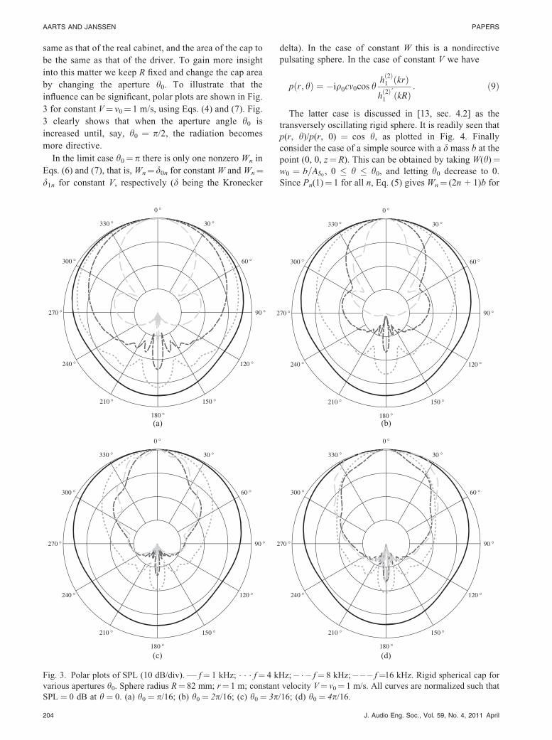
same as that of the real cabinet, and the area of the cap to

be the same as that of the driver. To gain more insight

into this matter we keep R fixed and change the cap area

by changing the aperture h0. To illustrate that the

influence can be significant, polar plots are shown in Fig.

3 for constant V¼ v0¼ 1 m/s, using Eqs. (4) and (7). Fig.

3 clearly shows that when the aperture angle h0 is

increased until, say, h0 ¼ p/2, the radiation becomes

more directive.

In the limit case h0¼ p there is only one nonzero Wn in

Eqs. (6) and (7), that is, Wn¼ d0n for constant W and Wn¼d1n for constant V, respectively (d being the Kronecker

delta). In the case of constant W this is a nondirective

pulsating sphere. In the case of constant V we have

pðr; hÞ ¼ �iq0cv0cos hhð2Þ1 ðkrÞ

hð2Þ 01 ðkRÞ

: ð9Þ

The latter case is discussed in [13, sec. 4.2] as the

transversely oscillating rigid sphere. It is readily seen that

p(r, h)/p(r, 0) ¼ cos h, as plotted in Fig. 4. Finally

consider the case of a simple source with a d mass b at the

point (0, 0, z¼R). This can be obtained by taking W(h)¼w0 ¼ b=AS0

, 0 � h � h0, and letting h0 decrease to 0.

Since Pn(1)¼ 1 for all n, Eq. (5) gives Wn¼ (2n þ 1)b for

Fig. 3. Polar plots of SPL (10 dB/div). — f¼ 1 kHz; � � � f¼ 4 kHz; – � – f¼ 8 kHz; – – – f¼16 kHz. Rigid spherical cap for

various apertures h0. Sphere radius R¼ 82 mm; r¼ 1 m; constant velocity V¼ m0¼ 1 m/s. All curves are normalized such that

SPL¼ 0 dB at h ¼ 0. (a) h0¼ p/16; (b) h0¼ 2p/16; (c) h0¼ 3p/16; (d) h0 ¼ 4p/16.



all n as h0 goes to 0, and there results

pðr; hÞ ¼ �iq0cbX‘

n¼0

ð2nþ 1ÞPnðcos hÞ hð2Þn ðkrÞ

hð2Þ 0n ðkRÞ

: ð10Þ

This case is illustrated in [23, fig. 3], from which it is

apparent that the responses at h¼ 0 and h¼ p are of the

same order of magnitude, especially at low frequencies.

This is discussed further in Section 3.2 in connection with

the acoustic center.

2 COMPARISON OF BAFFLE-STEP RESPONSES

At low frequencies the baffle of a loudspeaker is small

compared to its wavelength, and it radiates due to

diffraction effects in the full space (4p field). At those

low frequencies the radiator does not benefit from the

baffle in terms of gain. At high frequencies the

loudspeaker benefits from the baffle, which yields a gain

of 6 dB. This transition is the well-known baffle step. The

center frequency of this transition depends on the size of

the baffle. Olson [25] has documented this for 12 different

loudspeaker enclosures, including the sphere, cylinder,

and rectangular parallelepiped. All those 12 enclosures

share the common feature of increasing gain by about 6

dB when the frequency is increased from low to high. The

exact shape of this step depends on the particular

enclosure. For spheres the transition is smoothest, while

for other shapes undulations occur, in particular for

cabinets with sharp-edged boundaries. In Fig. 5(a) the

baffle step is shown for a polar cap (h0 ¼ p/8, constant

velocity V¼ v0¼1 m/s) on a sphere of radius R¼0.082 m

using Eqs. (4) and (7), for different observation angles h.

Compare the curves in Fig. 5(a) with the measurements

using the experimental loudspeaker [Fig. 5(b)], discussed

in Section 1, and that of a rigid piston in an infinite baffle

[Fig. 5(c)]. Using [12]–[14],

piðhÞpiðh ¼ 0Þ ¼

J1½ka sinðhÞ�½ka sinðhÞ� ð11Þ

for the normalized pressure. It appears that there is a

good resemblance between the measured frequency

response of the experimental loudspeaker and the polar

cap model. The undulations, for example, for h ¼ 3p/9

(dashed curve), at 7.4, 10, and 13.4 kHz correspond well.

Although these undulations are often attributed to the

nonrigid cone movement of the driver itself, our

illustrations show that it is mainly a diffraction effect.

Furthermore it can be observed that even on axis (h¼ 0)

there is a gradual decrease in SPL at frequencies above

about 10 kHz. It can be shown from the asymptotics of

the spherical Hankel functions that for h¼ 0, k! ‘, and

r � R, the sound pressure p(r, h) decays at least as

O(k�1/3). This is in contrast to a flat piston in an infinite

baffle [Fig. 5(c)]. There the on-axis pressure does not

decay, and the baffle step is absent. This is discussed

further at the end of Section 3.2. Although it is highly

speculative, and should be validated for different drivers

and cabinets, one might expect that the ratio of the

pressure of the cap using Eqs. (4) and (7) to that of the

piston in an infinite baffle using Eq. (11) can assist in

interpreting published loudspeaker response curves that

are measured under standardized (infinite-baffle) condi-

tions. For typical loudspeakers at low frequencies the

loss is theoretically 6 dB, but is counteracted by room

placement. A range of 3–6 dB is usually allowed. At

sufficiently high frequencies the piston does not benefit

from the baffle because it is highly directional. Finally

the tests were done using a high-quality 3.5-inch

loudspeaker. In such a unit the first cone breakup mode

usually occurs around 10 kHz. However, the present case

does not exhibit a clear breakup mode because it is very

well damped. This was verified by means of a PolyTec

PSV-300-H scanning vibrometer with an OFV-056 laser

head.

3 COMPARISON OF POWER AND DIRECTIVITY

3.1 Sound Power

The sound power is meaningful in various respects.

First it is used in efficiency calculations, which we do not

consider here. Second it is important with regard to sound

radiation. Different loudspeakers may share a common,

rather flat on-axis SPL response, while their off-axis

responses differ considerably. Therefore we consider the

power response important. We restrict ourselves to

axisymmetric drivers and we do not discuss horn

loudspeakers. The power is defined as the intensity pv*

Fig. 4. Polar plot for sphere (h0 ¼ p) moving with constant

velocity V¼ m0¼1 m/s in z direction. W1¼1; Wn¼0 for all n

6¼ 1.



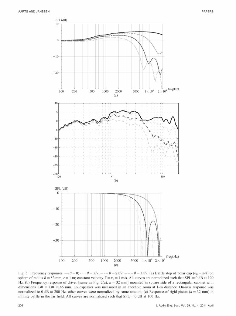
Fig. 5. Frequency responses. — h¼ 0; � � � h¼ p/9; – � – h¼ 2p/9; – – – h¼ 3p/9. (a) Baffle step of polar cap (h0¼ p/8) on

sphere of radius R¼ 82 mm, r¼ 1 m; constant velocity V¼ m0¼ 1 m/s. All curves are normalized such that SPL¼ 0 dB at 100

Hz. (b) Frequency response of driver [same as Fig. 2(a), a ¼ 32 mm] mounted in square side of a rectangular cabinet with

dimensions 130 3 130 3186 mm. Loudspeaker was measured in an anechoic room at 1-m distance. On-axis response was

normalized to 0 dB at 200 Hz, other curves were normalized by same amount. (c) Response of rigid piston (a ¼ 32 mm) in

infinite baffle in the far field. All curves are normalized such that SPL ¼ 0 dB at 100 Hz.



integrated over the sphere Sr of radius r � R,

P ¼Z

Sr

pv dSr ð12Þ

where p and v are pressure and velocity at an arbitrary

point on the sphere Sr. Using Eq. (4) for the pressure and

v ¼ �1

ikq0c

]p

]nð13Þ

we get

vðr; h;uÞ ¼X‘

n¼0

WnPnðcos hÞ hð2Þ 0n ðkrÞ

hð2Þ 0n ðkRÞ

: ð14Þ

By the orthogonality of the Legendre polynomials it

follows that

P ¼Z

Sr

pv dSr ¼ 2pZ p

0

pðr; hÞvðr; hÞr2sin h dh

¼ �iq0cX‘

n¼0

jWnj2

nþ 1

2

2pr2hð2Þn ðkrÞ½hð2Þ

0

n ðkrÞ�

hð2Þ 0n ðkRÞ

��2

: ð15Þ

Using [24, eq. 10.1.6],

W jnðzÞ; ynðzÞf g ¼ jnðzÞy0

nðzÞ � j0

nðzÞynðzÞ ¼1

z2ð16Þ

where W denotes the Wronskian, we get

<½P� ¼ 2pq0c

k2

X‘

n¼0

jWnj2

nþ 1

2

� �hð2Þ 0n ðkRÞ

��2: ð17Þ

Note that Eq. (17) has been derived without using any

(near-field or far-field) approximation. The real part of the

acoustic power is independent of r, which is in

accordance with the conservation of power law. For low

frequencies Eq. (17) is approximated as

<½P� ¼ 4pq0cW2

0 k2R

4: ð18Þ

To illustrate Eq. (17), the normalized power <[P]/2pq0cv2

0R2 is plotted in Fig. 6, where a cap with various

apertures is moving with constant velocity V¼ v0¼ 1 m/s

[using Eqs. (7) and (17)].

Next we compare the calculated power with the

power measured in a reverberation room using the

experimental loudspeaker discussed in Section 1. Here

we assumed the pole cap moving not with constant

velocity but with constant acceleration (V 0 ¼ ikcV),

corresponding to a frequency-independent current of

constant amplitude through the loudspeaker. Fig. 7

shows plots of the calculated power for a rigid spherical

cap moving with constant acceleration and at various

apertures, together with the power obtained from the

measured loudspeaker. It appears that the calculated

power for h0 ¼ p/8 and the power from the measured

loudspeaker are quite similar while there was no special

effort made to obtain a best fit. A slightly larger aperture

than the ‘‘round’’ value h0¼ p/8, which we use in many

examples in this paper, would have resulted in a better

fit. The low-frequency behavior of Fig. 7 follows

directly from multiplying Eq. (18) with 1/(kc)2 because

of the constant acceleration of the cap.

3.2 Directivity

The far-field pressure can be calculated by substituting

the asymptotic value [24, ch. 10]

hð2Þn ðkrÞ’ i

nþ1 e�ikr

krð19Þ

in Eq. (4), which leads to

pðr; hÞ’ q0ce�ikr

kr

X‘

n¼0

inWn

hð2Þ 0n ðkRÞ

Pnðcos hÞ: ð20Þ

In Kinsler et al. [12, sec. 8.9] the far-field relation is

written as

pðr; h;uÞ ¼ paxðrÞHðh;uÞ ð21Þ

in which pax(r) is the pressure at h ¼ 0, and H(h, u) is

Fig. 6. Power <[P]/2pq0cv20R2 of rigid spherical cap moving

with constant velocity V ¼ m0 ¼ 1 m/s for various apertures.

— h0¼5p/32; � � � h0¼p/8; – � – h0¼p/10. Sphere radius R¼82 mm.

Fig. 7. Power <[P]c/2pq0a20R4 [dB] versus kR (log axis) of

rigid spherical cap moving with constant acceleration V0 ¼ikcV for various apertures. — h0¼ 5p/32; � � � h0¼ p/8; – � –h0 ¼ p/10; irregular curve—Power from measured loud-

speaker. Sphere radius R ¼ 82 mm. Logarithmic horizontal

axis runs from kR¼ 0.1 to 20, corresponding to a frequency

range of 66 Hz to 13.2 kHz.



dimensionless with H(0, 0) ¼ 1. Since there is no udependence, we delete it. This leads to

paxðrÞ ¼ q0ce�ikr

kr

X‘

n¼0

inWn

hð2Þ 0n ðkRÞ

ð22Þ

and

HðhÞ ¼ pðr; hÞpaxðrÞ

¼

X‘

n¼0

inWn

hð2Þ 0n ðkRÞ

Pnðcos hÞ

X‘

n¼0

inWn

hð2Þ 0n ðkRÞ

: ð23Þ

The total radiated power P in the far field follows from

Eq. (12) and the far-field relation v ¼ p/q0c as

Y¼Z

Sr

1

q0cjpj2 dSr

¼ 1

q0cjpaxðrÞj

2r

2Z 2p

0

Z p

0

jHðhÞj2sin h dh du: ð24Þ

For a simple (nondirective) source at the origin to yield

the same acoustical power on Sr, the pressure ps should

satisfy

Y¼ 1

q0c4pr

2jpsðrÞj2: ð25Þ

Therefore the directivity defined as

D ¼ jpaxðrÞj2

jpsðrÞj2ð26Þ

follows from Eqs. (23)–(25), using the orthogonality of

the Legendre polynomials, as

D ¼ 2X‘

n¼0

inþ1Wn

hð2Þ 0n ðkRÞ

��

��

224

35X‘

n¼0

Wnj j2

nþ 1

2

� �hð2Þ 0n ðkRÞ

��2

2

664

3

775

�1

:

(27)

The directivity index DI ¼ 10 log10 D [dB] versus kR is

plotted in Fig. 8 for a cap moving with constant velocity

V. For comparison the directivity

Drp ¼ðkaÞ2

1� J1ð2kaÞ=kað28Þ

of a rigid piston in an infinite baffle [12] is plotted in Fig.

8 by the dashed curve starting at 3 dB (with ka¼ kR/2.5,

so that the p/8 cap and piston have the same area). At low

frequencies the directivity Drp is 3 dB because the piston

is radiating in the 2p field while the caps are radiating in

the 4p field. At higher frequencies the curve almost

coincides with the dotted curve, which corresponds to the

h0 ¼ p/8 cap.

Now consider the case where kR ! ‘. Then using

hð2Þ 0n (kR) ’ ine�ikR/kR, it follows that D is approximated

by

D ’

2X‘

n¼0

Wn

��

��

2

X‘

n¼0

jWnj2

nþ 1

2

¼ 2jWðh ¼ 0Þj2Z p

0

jWðhÞj2sin h dhð29Þ

or, in words, by the ratio of jW (h¼ 0)j2 to the average

value of jW(h)j2 over the sphere. Eqs. (27) and (29)

show that the directivity—which is a typical far-field

acoustical quantity—is fully determined in a simple

manner by the velocity profile of the pole cap, which

can be easily derived from measurements, such as with

a laser Doppler meter. This procedure is not discussed

here. A similar result was obtained for a flexible

radiator in an infinite flat baffle [10]. In the flat-baffle

case the directivity increases with (ka)2. For the cap

case there is indeed an initial increase with (kR)2, but at

very high frequencies there is a decrease in directivity.

In most cases these high frequencies are beyond the

audio range, but may be of importance for ultrasonics.

The deviation of the (kR)2 behavior appears in Fig. 8 for

h0 as low as 5p/32 (solid curve). This effect may seem

counterintuitive or even nonphysical. However, the on-

axis (h ¼ 0) pressure decreases for high frequencies as

well (see Fig. 5). This will decrease the numerator on

the right-hand side of Eq. (26). This effect does not

occur with a piston in an infinite baffle, which has a

constant, nondecreasing on-axis sound pressure, but a

narrowing beamwidth.

Fig. 8. Directivity index DI¼10 log10 D [dB] versus kR (log

axis) of rigid spherical cap for various apertures. — h0¼ 5p/

32; � � � h0¼ p/8; – � – h0¼ p/10. Constant velocity V; sphere

radius R¼ 82 mm. – – – curve starting at 3 dB is directivity

for rigid piston in an infinite baffle, using Eq. (28).

Logarithmic horizontal axis runs from kR ¼ 0.1 to 25,

corresponding to a frequency range of 66 Hz to 16.5 kHz.



4 ACOUSTIC CENTER

The acoustic center of a reciprocal transducer can be

defined as the point from which spherical waves seem to

be diverging when the transducer is acting as a source.

There are, however, additional definitions. See [26] for an

overview and discussion. This concept is used mainly for

microphones. Recently the acoustic center was discussed

[27], [28] for normal sealed-box loudspeakers as a

particular point that acts as the origin of the low-

frequency radiation of the loudspeaker. At low frequen-

cies the radiation from such a loudspeaker becomes

simpler as the wavelength of the sound becomes larger

relative to the enclosure dimensions, and the system

behaves externally as a simple source (point source). The

difference between the origin and the true acoustic center

is denoted by D. If p(r, 0) and p(r, p) are the sound

pressure in front and at the back of the source, then Dfollows from

jpðr; 0Þjr þ D

¼ jpðr; pÞjr � D

ð30Þ

as

D ¼ rjqj � 1

jqj þ 1ð31Þ

where

q ¼ pðr; 0Þpðr; pÞ : ð32Þ

The pole-cap model is used to calculate the function q via

Eq. (4); see Fig. 9.

Subsequently this model is used to compute the

acoustic center with Eq. (31). Assume that kR 1 and

R/r 1, and also that Wn is real with Wn of at most the

same order of magnitude as W0. Then two terms of the

series in Eq. (4) are sufficient, and using Pn(1) ¼ 1 and

Pn(�1) ¼ (�1)n, q can be written as

q ’ W0

hð2Þ0 ðkrÞ

hð2Þ 00 ðkRÞ

þW1

hð2Þ1 ðkrÞ

hð2Þ 01 ðkRÞ

" #

3 W0

hð2Þ0 ðkrÞ

hð2Þ 00 ðkRÞ

�W1

hð2Þ1 ðkrÞ

hð2Þ 01 ðkRÞ

" #�1

: ð33Þ

Because kR 1, the small argument approximation of

the spherical Hankel functions

hð2Þ 00 ðzÞ’

�i

z2; h

ð2Þ 01 ðzÞ’

�2i

z3ð34Þ

can be used, and together with the identity

hð2Þ1 ðkrÞ

hð2Þ0 ðkrÞ

¼ 1

krð1þ ikrÞ ð35Þ

we get

q ’ 1þ W1

2W0

ð1þ ikrÞRr

� �1� W1

2W0

ð1þ ikrÞRr

� ��1

:

(36)

By our assumptions we have

W1

2W0

ð1þ ikrÞRr

��

�� 1

and so

q ’ 1þW1

W0

R

rð1þ ikrÞ: ð37Þ

Finally assuming that

ðkrÞ2 2W0

W1

��

��r

R;

Fig. 9. Function 20 log10 jqj [dB] versus kR (log axis) [Eq. (32)] of rigid spherical cap for various apertures. — h0¼5p/32; � � �h0¼p/8; – � – h0¼p/10; – – – simple source on sphere using Eq. (10). Constant velocity V, all at r¼ 1 m; sphere radius R¼ 82

mm. Solid circles—real driver [same as Fig. 2(a); a¼ 32 mm] mounted in square side of a rectangular cabinet. Logarithmic

horizontal axis runs from kR ¼ 0.02 to 30, corresponding to a frequency range of 13 Hz to 19.8 kHz.



there holds

jqj’ 1þW1

W0

R

rð38Þ

and if W1R/W0r 1 there holds

uq ¼ arg q ’ arctanW1

W0

xR

cð39Þ

where it has been used that W1/W0 is real and k ¼ x/c.

Substitution of Eq. (38) into Eq. (31) results in

D ’RW1

2W0

: ð40Þ

Note that this result is real, independent of k and r, and

only mild assumptions were used. The delay between the

front and the back of the source is equal to s ¼ duq/dx.

Using Eqs. (39) and (40), and assuming kR W0/W1 we

get

s ’2Dc: ð41Þ

For the case where W is constant the Wn follow from Eq.

(6), resulting in

D ’3

4Rð1þ cos h0Þ: ð42Þ

If h0 ¼ p and W is constant, the radiator is a pulsating

sphere and, according to Eq. (42), has its acoustical center

at the origin. For the case V is constant the Wn follow

from Eq. (7), resulting in

D ’ R cos h0 þ1

1þ cos h0

� �: ð43Þ

If h0¼ p and V is constant, the notion of acoustical center

does not make sense because of the notches in the polar

plot at low frequencies (see Fig. 4). The absolute error in

the approximation of D/R by Eq. (43) (for f¼1 Hz, R¼82

mm, r¼ 100 m, and 0 � h0 � p/2) is , 5 3 10�7. Fig. 9

shows that for a cap moving with constant velocity V the

low-frequency asymptote is flat to about kR ¼ 0.4,

corresponding to 264 Hz. Hence the approximation of D/

R by Eq. (43) is rather accurate up to this frequency. The

relative acoustic center difference D/R versus h0 is plotted

in Fig. 10 for constant W and V, using Eqs. (42) and (43).

Note that D/R¼3/2 for h0¼0 in both cases and that V and

W are constant. This agrees with what would be given by

the simple source on a sphere [see Eq. (10)]. We have W0

¼ 1 and W1¼ 3, and by Eq. (40) we obtain D/R¼ 3/2. For

low frequencies this is also shown in [26, fig. 3, eqs. 18–

19]. Further it appears that for modest apertures, say, h0

� 0.5, the difference between the right-hand sides of Eqs.

(42) and (43) is very small, on the order of h40. From this

we may conclude that—at low frequencies (kR � 0.4)—

the acoustic center for a loudspeaker lies about 0–0.5R in

front of the loudspeaker, where R is the radius in the case

of a spherical cabinet, or some other dimensional measure

of the cabinet. At higher frequencies the acoustic center

shifts further away from the loudspeaker. For example,

between kR¼1 (660 Hz) and kR¼ 2 (1.32 kHz) q is about

5 dB (see Fig. 9), corresponding to D ¼ 3.4R ¼ 280 mm

[using Eq. (31)].

The polar response jp(r, h)/p(r, 0)j at low frequencies

can be computed in a similar way as q in Eq. (36). The

minus sign in the denominator on the right-hand side of

Eq. (36) is due to P1(cos p)¼�1. Using now P1(cos h)¼cos h and interchanging the numerator and denominator

of Eq. (36) yields

pðr; hÞpðr; 0Þ’ 1þ W1

2W0

ð1þ ikrÞRr

cos h

� �

3 1þ W1

2W0

ð1þ ikrÞRr

� ��1

: ð44Þ

Assuming that

ðkrÞ2 2W0

W1

��

��r

R;

Eq. (44) can be approximated by

pðr; hÞpðr; 0Þ

��

��’ 1þ ðcos h� 1Þ W1

2W0

R

r: ð45Þ

Eq. (45) clearly shows that the deviation from omnidi-

rectional radiation is proportional to the ratios W1/2W0

and R/r while it is independent of frequency for low

frequencies. For fixed W1/2W0 and R/r the polar pattern is

not truly omnidirectional at low frequencies. This is

because the acoustic center does not coincide with the

origin in general.

5 CONCLUSIONS AND OUTLOOK

The polar plot of a rigid spherical cap on a rigid sphere

has been shown to be quite similar to that of a real

loudspeaker (see Fig. 2) and is useful in the full 4p field.

It thus outperforms the more conventional model in which

the loudspeaker is modeled as a rigid piston in an infinite

baffle. The cap model can be used to predict, besides

polar plots, various other acoustical quantities of a

loudspeaker. These quantities include sound pressure,

baffle-step response, sound power, directivity, and the

Fig. 10. Relative acoustic center difference D/R versus h0.

— using Eq. (42) for W constant; � � � using Eq. (43) for V¼m0¼ 1 m/s constant.



acoustic center. The baffle-step response of the model is

rather similar to that of a loudspeaker (see Fig. 5). The

sound power predicted by the model is very similar to that

of a loudspeaker measured in a reverberation room (see

Fig. 7). The directivity D given by the model is

approximated as the ratio of jW (h ¼ 0)j2 to the average

value of jW (h)j2 over the sphere [see Eq. (29)]. The ratio

of the sound pressure in front and at the back of the

loudspeaker, which is associated with the acoustic center,

is for a loudspeaker very similar to that given by the

model (see Fig. 9). At low frequencies the acoustic center

for a loudspeaker lies about 0–0.5 times the sphere radius

in front of the loudspeaker (see Fig. 10). At higher

frequencies the acoustic center shifts further away from

the loudspeaker. All results are obtained using one

loudspeaker only. The value of this model for other

drivers in other cabinets should be tested in order to

derive bounds for the applicability of the model. This

work remains to be done in the future.

6 ACKNOWLEDGMENT

The authors dedicate this paper to Mrs. Doortje Aarts-

Ultee, who at age 53, passed away 2009 August 6, while

this paper was taking shape. The authors wish to thank

Okke Ouweltjes for assisting with the loudspeaker

measurements and making the plot for Fig. 2(a), and the

reviewers for pertinent suggestions, which made the paper

considerably more readable.

7 REFERENCES

[1] J. W. S. Rayleigh, The Theory of Sound, vol. 2,

(1896; reprinted by Dover, New York, 1945).

[2] L. V. King, ‘‘On the Acoustic Radiation Field of the

Piezo-Electric Oscillator and the Effect of Viscosity on

Transmission,’’ Can. J. Res., vol. 11, pp. 135–155 (1934).

[3] M. Greenspan, ‘‘Piston Radiator: Some Extensions

of the Theory,’’ J. Acoust. Soc. Am., vol. 65, pp. 608–621

(1979 March).

[4] G. R. Harris, ‘‘Review of Transient Field Theory for

a Baffled Planar Piston,’’ J. Acoust. Soc. Am., vol. 70, pp.

10–20 (1981 July).

[5] T. Hasegawa, N. Inoue, and K. Matsuzawa, ‘‘ANew Rigorous Expansion for the Velocity Potential of a

Circular Piston Source,’’ J. Acoust. Soc. Am., vol. 74, pp.

1044–1047 (1983 Sept.).

[6] D. A. Hutchins, H. D. Mair, P. A. Puhach, and A. J.

Osei, ‘‘Continuous-Wave Pressure Fields of Ultrasonic

Transducers,’’ J. Acoust. Soc. Am., vol. 80, pp. 1–12

(1986 July).

[7] R. C. Wittmann, and A. D. Yaghjian, ‘‘Spherical-

Wave Expansions of Piston-Radiator Fields,’’ J. Acoust.

Soc. Am., vol. 90, pp. 1647–1655 (1991 Sept.).

[8] T. J. Mellow, ‘‘On the Sound Field of a Resilient

Disk in an Infinite Baffle,’’ J. Acoust. Soc. Am., vol. 120,

pp. 90–101 (2006 July).

[9] R. M. Aarts and A. J. E. M. Janssen, ‘‘On-Axis and

Far-Field Sound Radiation from Resilient Flat and Dome-

Shaped Radiators,’’ J. Acoust. Soc. Am., vol. 125, pp.

1444–1455 (2009 March).

[10] R. M. Aarts and A. J. E. M. Janssen, ‘‘Sound

Radiation Quantities Arising from a Resilient Circular

Radiator,’’ J. Acoust. Soc. Am., vol. 126, pp. 1776–1787

(2009 Oct.).

[11] P. M. Morse and K. U. Ingard, Theoretical

Acoustics (McGraw-Hill, New York, 1968).

[12] L. E. Kinsler, A. R. Frey, A. B. Coppens, and J. V.

Sanders, Fundamentals of Acoustics (Wiley, New York,

1982).

[13] A. D. Pierce, Acoustics—An Introduction to Its

Physical Principles and Applications (Acoustical Society

of America through the American Institute of Physics,

1989).

[14] D. T. Blackstock, Fundamentals of Physical

Acoustics (Wiley, New York, 2000).

[15] H. Suzuki and J. Tichy, ‘‘Sound Radiation from

Convex and Concave Domes in an Infinite Baffle,’’ J.

Acoust. Soc. Am., vol. 69, pp. 41–49 (1981 Jan.).

[16] H. Suzuki and J. Tichy, ‘‘Radiation and Diffraction

Effects of Convex and Concave Domes,’’ J. Audio Eng.

Soc., vol. 29, pp. 873–881 (1981 Dec.).

[17] P. M. Morse and H. Feshbach, Methods of

Theoretical Physics (McGraw-Hill, New York, 1953).

[18] H. Stenzel and O. Brosze, Guide to Computation

of Sound Phenomena (published in German as Leitfaden

zur Berechnung von Schallvorgangen), 2nd ed. (Springer,

Berlin, 1958).

[19] E. Skudrzyk, The Foundations of Acoustics

(Springer, New York, 1971; reprinted by Acoustical

Society of America, 2008).

[20] R. New, R. I. Becker, and P. Wilhelmij, ‘‘A

Limiting Form for the Nearfield of the Baffled Piston,’’ J.

Acoust. Soc. Am., vol. 70, pp. 1518–1526 (1981 Nov.).

[21] P. H. Rogers and A. O. Williams, Jr., ‘‘Acoustic

Field of Circular Plane Piston in Limits of Short

Wavelength or Large Radius,’’ J. Acoust. Soc. Am., vol.

52, pp. 865–870 (1972 Sept.).

[22] T. Helie and X. Rodet, ‘‘Radiation of a Pulsating

Portion of a Sphere: Application to Horn Radiation,’’ Acta

Acustica/Acustica, vol. 89, pp. 565–577 (2003 July/Aug.).

[23] R. M. Aarts and A. J. E. M. Janssen, ‘‘Sound

Radiation from a Resilient Spherical Cap on a Rigid

Sphere,’’ J. Acoust. Soc. Am., vol. 127, pp. 2262–2273

(2010 Apr.).

[24] M. Abramowitz and I. A. Stegun, Handbook of

Mathematical Functions (Dover, New York, 1972).

[25] H. F. Olson, ‘‘Direct Radiator Loudspeaker

Enclosures,’’ J. Audio Eng. Soc., vol. 17, pp. 22–29

(1969 Jan.).

[26] F. Jacobsen, S. Barrera Figueroa, and K.

Rasmussen, ‘‘A Note on the Concept of Acoustic Center,’’

J. Acoust. Soc. Am., vol. 115, pp. 1468–1473 (2004 Apr.).

[27] J. Vanderkooy, ‘‘The Acoustic Center: A New

Concept for Loudspeakers at Low Frequencies,’’ present-

ed at the 121st Convention of the Audio Engineering



Society, J. Audio Eng. Soc. (Abstracts), vol. 54, p. 1261

(2006 Dec.), convention paper 6912.

[28] J. Vanderkooy, ‘‘The Low-Frequency Acoustic

Center: Measurement, Theory, and Application,’’

presented at the 128th Convention of the Audio Engi-

neering Society, (Abstracts) www.aes.org/events/128/

128thWrapUp.pdf, (2010 May), convention paper

7992.

THE AUTHORS

R. M. Aarts A. J. E. M. Janssen

Ronald M. Aarts was born in Amsterdam, The

Netherlands in 1956. He received a B.Sc. degree in

electrical engineering in 1977 and a Ph.D. degree in

physics from Delft University of Technology in 1995.

He joined the Optics Group at Philips Research

Laboratories, Eindhoven, The Netherlands, in 1977 and

initially investigated servos and signal processing for use

in both Video Long Play players and Compact Disc

players. In 1984 he joined the Acoustics Group at Philips

Research Laboratories and worked on the development of

CAD tools and signal processing for loudspeaker systems.

In 1994 he became a member of the Digital Signal

Processing (DSP) Group at Philips Research Laboratories

and has led research projects on the improvement of

sound reproduction by exploiting DSP and psychoacous-

tical phenomena. In 2003 he became a Research Fellow at

the Philips Research Laboratories and extended his

interests in engineering to medicine and biology. He is

part-time full professor at the Eindhoven University of

Technology.

Dr. Aarts has published a large number of papers and

reports and holds over 150 first patent application filings,

including over 35 granted US patents in the aforemen-

tioned fields. He has served on a number of organizing

committees and as chairman for various international

conventions. He is a Fellow of the IEEE, a Silver Medal

recipient, Fellow, and past governor of the Audio

Engineering Society, a member of the Dutch Acoustical

Society, the Acoustical Society of America, the Dutch

Society for Biophysics and Biomedical Engineering, and

the Dutch Society for Sleep and Wake Research.

X

Augustus J. E. M. Janssen received engineering and

Ph.D. degrees in mathematics from the Eindhoven

University of Technology, The Netherlands, in 1976

and 1979, respectively. From 1979 to 1981 he was a

Bateman Research Instructor in the Mathematics Depart-

ment of the California Institute of Technology. From

1981 until 2010 he worked with Philips Research

Laboratories, Eindhoven, where his principal responsibil-

ity was to provide high-level mathematical service and

consultancy in mathematical analysis. He is currently

affiliated with the Departments of Mathematics (EUR-

ANDOM) and of Electrical Engineering at the Eindhoven

University of Technology, where he provides consultancy

in mathematical analysis.

Dr. Janssen has published over 180 papers in the fields

of Fourier analysis, signal analysis, time–frequency

analysis, electron microscopy, optical diffraction theory,

and queueing theory. His current interests include the

application of techniques from the theory of optical

aberrations to the characterization of acoustical radiators.

He is a Fellow of the IEEE.



Documents

Comparing Sound Radiation from a Loudspeaker with … Sound Radiation from a Loudspeaker ... with the advantage ... equal volume, the polar plot corresponding to thePublished in: Journal