Embed Size (px)
Citation preview
Comparing satellite derived rainfall
with ground based radar for
North-western Europe
Hojjat Seyyedi
January, 2010

Course Title: Geo-Information Science and Earth Observation
for Environmental Modelling and Management
Level: Master of Science (Msc)
Course Duration: April 2008 - January 2010
Consortium partners: University of Southampton (UK)
Lund University (Sweden)
University of Warsaw (Poland)
International Institute for Geo-Information Science
and Earth Observation (ITC) (The Netherlands)
GEM thesis number: 2010-04

Comparing satellite derived rainfall with ground based radar for North-western
Europe
by
HOJJAT SEYYEDI
Thesis submitted to the International Institute for Geo-information Science and Earth
Observation in partial fulfilment of the requirements for the degree of Master of
Science in Geo-information Science and Earth Observation for Environmental
Modelling and Management
Thesis Assessment Board
Chairman: Prof.Dr. Z. (Bob) Su
External Examiner: Prof T.P. Dawson
Internal Examiner: Dr. B.H.P. (Ben) Maathuis
Supervisor: Dr.Ir. C.M.M. (Chris) Mannaerts
Supervisor: M.Sc. A. (Andre) Kooiman
International Institute for Geo-Information Science and Earth Observation
Enschede, The Netherlands

Disclaimer
This document describes work undertaken as part of a programme of study at
the International Institute for Geo-information Science and Earth Observation.
All views and opinions expressed therein remain the sole responsibility of the
author, and do not necessarily represent those of the institute.
i
Abstract
The primary reason of implementing meteorological satellites is avoid the coverage
and time gap of conventional ground-based rainfall data for a number of
applications, above all hydrology and weather forecasting and finally enhanced
identification and quantification of rainfall at the time scales. Uses of global and
local data have significant limitation because of lack of precipitation measurements
over the oceans as well as uneven distribution of rain gauges and weather radars
over land. Precipitation has also a direct impact on human life that other atmospheric
phenomena seldom have: an example is represented by heavy rain events and flash
floods (Levizzani et al., 2002). According to above background satellite
precipitation estimates are widely used to measure global rainfall on near real-time
and monthly timescales for climate studies, numerical weather prediction (NWP)
data assimilation, now-casting and flash flood warning, tropical rainfall potential,
and water resources monitoring. Therefore similar to any observational data,
investigating their accuracy and limitations is crucial. This is done by verifying the
satellite estimates against independent data from rain gauges and radars (Levizzani,
et al., 2007). The study utilized two METEOSAT products that are currently freely
available to the scientific community: multi sensor precipitation estimate (MPE)
from METEOSAT8 with 5 minutes temporal resolution and MPE from
METEOSAT9 with 15 min temporal resolution. The gauge adjusted radar
precipitation measurements with 5 minutes temporal resolution from the royal
Netherlands meteorological institute (KNMI) used as reference data. All data series
were collected and processed for two different rainfall events over the Netherlands
and some parts of Belgium. Two types of statistical analysis have been applied,
categorical statistics to assess the special accuracy of products as well as continuous
statistics to assess errors in magnitude. The statistical analysis has been done based
on three different temporal resolutions, instantaneous, one hour accumulated and
three hours accumulated. The categorical statistical scores for the MPE products
from METEOSAT8 and METEOSAT9 have been improved by decreasing temporal
resolution from 15 min to 3 hours accumulated. These values for the first event are
better than the second event. This indicates these products have some difficulty in
estimating severe events. However, the METEOSAT8 MPE product has relatively
better performance in case of second event. May be this is related to shorter
accumulation time for the co-location with the SSM/I which leads to higher
performance in severe events. In case of the first event the MPE product from
METEOSAT9 shows higher scores. It is easy to infer that in normal rainfall events
using MPE product from METEOSAT9 is more reliable. The null hypothesis of

ii
there is no difference in spatial accuracy of EUMETSAT MPE products from
METEOSAT8 and METEOSAT9 rejected. Regression analysis for mean rainfall
values indicates in case of first event the r² is roughly 0.90 with 95% confidence
level. This shows very strong correlation between MPE products and ground based
radar data. However, this value for the second event is roughly 60% with 95%
confidence level. These results confirm the weakness of MPE products in estimating
severe events. It is worth to mention that the mean rainfall values from
METEOSAT9 MPE product has relatively higher correlation with ground based
radar data in all cases. The time series graphs related to ME, MAE and RMSE shows
overestimation in MPE products. The overestimation is almost the same for both
products. The magnitude of overestimation in the second event is drastically more
than the first event. These graphs also are in the same direction with the previous
results, and verify the limitation of MPE products in estimating strong events. The
null hypothesis of There is no difference in estimated values by EUMETSAT MPE
products from METEOSAT8 and METEOSAT9 rejected.

iii
Acknowledgements
Foremost, I would like to express my sincere gratitude to European Union, Erasmus
Mundus consortium and GEM MSc course organizers from the University of
Southampton, the Lund University, Warsaw University and the ITC, for awarding
me the scholarship to undertake this course. It has been a lifetime experience for me.
I owe my deepest gratitude to my first supervisor Dr. Ben Maathuis. Thank you very
much for your continuous support, guidance and useful suggestions during my
research. I gained a lot of scientific experience from him. I was overwhelmed by his
patience and the encouragement that he gave me from the beginning of the work
until production of the thesis. I am most grateful to my second supervisor Dr. Chris
Mannaerts for his continuous supports, enthusiasm, and immense knowledge.
My special thanks to Prof Beth Ebert, Chief Scientist, The Centre for Australian
Weather and Climate Research, Dr. Thomas Heinemann, Meteorological Product
Expert, EUMETSAT, Germany, dr. I. Holleman and Dr. Rob Roebeling, Chief
Scientist, Royal Netherlands Meteorological Institute, Dr. Angel Luque, Universitat
de les Illes Balears, and Mr. Bas Retsios, ITC, for their invaluable support and
suggestions on data sets processing and statistical analysis.
My sincere thanks also goes to Prof. T.P. Dawson, Prof. Andrew Skidmore, Prof.
Katarzyna Dobrowska, Prof. Petter Pilesjö, Dr. Cecilia Akselsson, Mr. Andre
Kooiman, Ms. Karin Larsson, Ms. Steff Webb and Ms. Monique Romarck for their
support and hospitality during my stay in four hosting countries.
My best wishes to my GEM classmates from around the globe and the lovely people
whom I met in the four countries for sharing their friendship and knowledge during
the past 18 months.
Last but not the least; I would like to thank my family: my parents Esmaeil Seyyedi
and Iran Badri for giving birth to me at the first place and supporting me spiritually
throughout my life. Behnam, Maryam, and Fatima, thanks for being supportive and
caring siblings.

iv
Table of contents
1. Introduction .......................................................................................... 13
1.1. Background and the problem........................................................ 13
1.2. Research objective ........................................................................ 15
1.2.1. General objective .................................................................. 15
1.2.2. Specific objectives ................................................................ 15
1.3. Research questions ....................................................................... 15
1.4. Research hypotheses ..................................................................... 15
1.5. Outline of the thesis ...................................................................... 17
2. Literature Review ................................................................................. 18
2.1. Satellite based precipitation estimation ........................................ 18
2.1.1. Visible and Infrared .............................................................. 18
2.1.2. Passive Microwave ............................................................... 19
2.1.3. Active sensors ....................................................................... 20
2.1.4. Blended techniques ............................................................... 21
2.2. Statistical methods for verifying estimated precipitation by
satelltes ..................................................................................................... 24
2.2.1. Validation of near real-time vs. climate scale precipitation . 24
2.2.2. Validation data ..................................................................... 25
2.2.3. Standard statistical methods for verifying precipitation
estimated by satellite ............................................................................ 25
3. Materials and methods .......................................................................... 30
3.1. General description of data ........................................................... 30
3.1.1. Description of EUMETSAT Multi Sensor Precipitation
Estimation (MPE) products .................................................................. 30
3.1.2. Description of ground based radar data ................................ 33
3.2. Methodology for comparision the satellite estimates against
independent data from radars ................................................................... 37
3.2.1. Data preparation ................................................................... 37
3.2.2. Categorical verification statistics ......................................... 39
3.2.3. Continuous verification statistics ......................................... 39
4. Results .................................................................................................. 43
4.1. The first event ............................................................................... 43
4.1.1. Instantaneous comparison .................................................... 45

v
4.1.2. One hour accumulated rainfall comparison .......................... 50
4.1.3. Three hours accumulated rainfall comparison...................... 55
4.2. The second event .......................................................................... 61
4.2.1. Instantaneous comparison .................................................... 61
4.2.2. One hour accumulated rainfall comparison .......................... 67
4.2.3. Three hours accumulated rainfall comparison...................... 72
5. Discussion ............................................................................................ 77
5.1. Spatial Accuracy........................................................................... 77
5.2. Assessing errors in magnitude ...................................................... 80
6. Conclusions and Recommendations ..................................................... 83
6.1. Conclusions .................................................................................. 83
6.2. Recommendations ........................................................................ 84
7. References ............................................................................................ 85
8. Appendix .............................................................................................. 89

vi
List of figures
Figure 1 the electromagnetic spectrum, from gamma rays to radio waves, on
satellite images of particular wavelengths .................................................... 18
Figure 2 Block diagram for both the real time and research product
algorithms, showing input data (left side), processing (center), output data
(right side), data flow (thin arrows), and processing control (thick arrows) 22
Figure 3 Look-up tables (LUT) derived from a 6h period on Aug. 19th, 2001
for the 5°x5° box number 229, over West Africa ......................................... 24
Figure 4 (a) EUMETSAT MPE product from METEOSAT8 (26th May 2009,
02:45 UTC). (b) EUMETSAT MPE product from METEOSAT9 (26th May
2009, 02:45 UTC) ........................................................................................ 32
Figure 5 Map shows KNMI weather radars location ................................... 33
Figure 6 (a) Radar reflectivity factor(dBZ) map and (b) Radar rainfall
intensity (mm/h) map for 26 May 2009, 00:00 UTC ................................... 36
Figure 7 the research methodology .............................................................. 37
Figure 8 processed images (a) MPE_METEOSAT9, (b)
MPE_RSS_METEOSAT8 and (c) RADAR (26 May 2009, 04:00 UTC) ... 39
Figure 9 flow diagram of methodology for categorical verification statistics
calculation .................................................................................................... 41
Figure 10 flow diagram of methodology for continuous verification statistics
calculation .................................................................................................... 42
Figure 11 reported rainfall for May 2009 ..................................................... 43
Figure 12 the cloud analysis image for the first event .................................. 44
Figure 13 mean rainfall values (Event1, instantaneous) .............................. 48
Figure 14 Mean Error (ME) values (Event1, instantaneous)........................ 48
Figure 15 Mean Absolute Error values (Event1, instantaneous) .................. 49
Figure 16 Root Mean Square Error (RMSE) values (Event1, instantaneous)
...................................................................................................................... 49
Figure 17 mean rainfall values (Event1, 1Hour accumulated) ..................... 53
Figure 18 Mean Error (ME) values (Event1, 1Hour accumulated) .............. 54
Figure 19 Mean Absolute Error values (Event1, 1Hour accumulated) ........ 54
Figure 20 Root Mean Square Error (RMSE) values (Event1, 1Hour
accumulated) ................................................................................................ 55
Figure 21 mean rainfall values (Event1, 3Hours accumulated) ................... 59

vii
Figure 22 Mean Error (ME) values (Event1, 3Hours accumulated) ............ 59
Figure 23 Mean Absolute Error values (Event1, 3Hours accumulated) ....... 60
Figure 24 Root Mean Square Error (RMSE) values (Event1, 3Hours
accumulated) ................................................................................................ 60
Figure 25 the cloud analysis image for the second event ............................. 61
Figure 26 mean rainfall values (Event2, instantaneous) .............................. 65
Figure 27 Mean Error (ME) values (Event2, instantaneous)........................ 65
Figure 28 Mean Absolute Error (MAE) values (Event2, instantaneous) ..... 66
Figure 29 Root Mean Square Error (RMSE) values (Event2, instantaneous)
...................................................................................................................... 66
Figure 30 mean rainfall values (Event2, 1 Hour accumulated) .................... 70
Figure 31 Mean Error (ME) values (Event2, 1 Hour accumulated) ............. 70
Figure 32 Mean Absolute Error (MAE) values (Event2, 1 Hour accumulated)
...................................................................................................................... 71
Figure 33 Root Mean Square Error (RMSE) values (Event2, 1 Hour
accumulated) ................................................................................................ 71
Figure 34 mean rainfall values (Event2, 3 Hours accumulated) .................. 75
Figure 35 Mean Error (ME) values (Event2, 3 Hours accumulated) ........... 75
Figure 36 Mean Absolute Error (MAE) values (Event2, 3Hours
accumulated) ................................................................................................ 76
Figure 37 Root Mean Square Error (RMSE) values (Event2, 3Hours
accumulated) ................................................................................................ 76
Figure 38 Scatter graph for MPE products, instantaneous comparison,
second event ................................................................................................. 81

viii
List of tables
Table 1 2*2 contingency table ..................................................................... 26
Table 2 MSG SERVI Channel ..................................................................... 30
Table 3 geographical projection parameters of the KNMI radar images.
Modified from .............................................................................................. 34
Table 4 the corners of KNMI radar image ................................................... 34
Table 5 Derived empirical constants a and b using the typical Z = aRb
relation, for several precipitation types ........................................................ 35
Table 6 calculated categorical statistics scores between METEOSAT8_RSS
and ground based radar (Event1, instantaneous) .......................................... 46
Table 7 calculated categorical statistics scores between METEOSA9 and
ground based radar (Event1, instantaneous) ................................................. 47
Table 8 calculated categorical statistics scores between METEOSAT8_RSS
and ground based radar (Event1, 1 Hour accumulated) ............................... 51
Table 9 calculated categorical statistics scores between METEOSA9 and
ground based radar (Event1, 1 Hour accumulated) ...................................... 53
Table 10 calculated categorical statistics scores between METEOSAT8_RSS
and ground based radar (Event1, 3 Hours accumulated) .............................. 57
Table 11 calculated categorical statistics scores between METEOSA9 and
ground based radar (Event1, 3Hours accumulated) ..................................... 58
Table 12 calculated categorical statistics scores between METEOSAT8_RSS
and ground based radar (Event2, instantaneous) .......................................... 63
Table 13 calculated categorical statistics scores between METEOSA9 and
ground based radar (Event2, instantaneous) ................................................. 64
Table 14 calculated categorical statistics scores between METEOSAT8_RSS
and ground based radar (Event2, 1 Hour accumulated) ............................... 68
Table 15 calculated categorical statistics scores between METEOSA9 and
ground based radar (Event2, 1 Hour accumulated) ...................................... 69
Table 16 calculated categorical statistics scores between METEOSAT8_RSS
and ground based radar (Event2, 3Hours accumulated) ............................... 73
Table 17 calculated categorical statistics scores between METEOSA9 and
ground based radar (Event2, 3Hours accumulated) ..................................... 74
Table 18 results for categorical statistics analysis (instantaneous) .............. 78
Table 19 results for categorical statistical analysis (one hour accumulated) 79

ix
Table 20 results for categorical statistical analysis (three hours accumulated)
...................................................................................................................... 79
Table 21 Regressions for mean rainfall values in MPE products,
instantaneous comparison, α=0.05 ............................................................... 81
Table 22 Regressions for mean rainfall values in MPE products, one hour
accumulated, α=0.05 .................................................................................... 82
Table 23 Regressions for mean rainfall values in MPE products, three hours
accumulated, α=0.05 .................................................................................... 82

x
Abbreviations
AMSR-E Advance Microwave Scanning Radiometer - Earth Observing
System
AMSU-B Aqua and Advance Microwave Sounding Unit – B
CAMS Climate Assesment and Monitoring System
CLAI Cloud Analysis Image
CPC Climate Prediction Center
CSI Critical Success Index
DMSP Defence Meteorological Satellite Program
DSD Drop Size Distribution
EBBT Equivalent Blackbody Temperature
ESA European Space Agency
ETS Equitable Threat Score
EUMETSAT European Organization for the Exploitation of Meteorological
Satellites
FAR False Alarm Ratio
FRC Fraction Correct
GDAL Geospatial Data Abstraction Library
GEO Geosynchronous
GMS Geostationary Meteorological Satellite
GOES Geostationary Operational Environmental Satellite
GPCC Global Precipitation Climatological Center
GPCP Global Precipitation Climatology Project
GPI GOES Precipitation Index
GPROF Goddard Profiling
GRIB GRIdded Binary
HDF5 Hierarchical Data Format 5
HRV High Resolution Visible
ILWIS Integrated Land and Water Information System
IR Infrared
ITC International Institute for Geo-Information Science and Earth
Observation
JAXA Japan Aerospace Exploration Agency
KNMI Royal Netherlands Meteorological Institute
LEO Low Earth Orbit
LUT Look up Table
MAE Mean Absolute Error

xi
ME Mean Error
METEOSAT Meteorological Satellite
MPE Multi-Sensor Precipitation Estimate
MSG Meteosat Second Generation
NIR Near Infrared
NOAA National Oceanic and Atmospheric Administration
NWP Numerical Weather Prediction
PERSIANN Precipitation Estimation from Remotely Sensed Information using
Artificial Neural Networks
PMW Passive Microwave
POD Probability of Detection
PR Precipitation Radar
pseudoCAPPI pseudo-Constant Altitude Plan Position Indicator
QPF Quantitative Precipitation Forecasting
RADAR Radio Detection and Ranging
RMSE Root Mean Square Error
RSS Rapid Scanning Service
SEVIRI Spinning Enhanced Visible and Infrared Imager
SI International System of Units
SSM/I Special Sensor Microwave/Imager
TMI TRMM Microwave Imager
TMPA TRMM Multi-satellites Precipitation Analysis
TRMM Tropical Rainfall Measuring Mission
UTC Universal Time Coordinate
UTM Universal Transverse Mercator
VIS Visible
WGS World Geodetic System
WMO World Meteorological Organization
WV Water Vapor
WWRP World Weather Research Program


13
1. Introduction
1.1. Background and the problem
The primary reason of implementing meteorological satellites is avoid the coverage
and time gap of conventional ground-based rainfall data for a number of
applications, above all hydrology and weather forecasting and finally enhanced
identification and quantification of rainfall at the time scales. Uses of global and
local data have significant limitation because of lack of precipitation measurements
over the oceans as well as uneven distribution of rain gauges and weather radars
over land. There is similar problem for the determination of wind, pressure,
temperature, and humidity fields. Precipitation has also a direct impact on human
life that other atmospheric phenomena seldom have: an example is represented by
heavy rain events and flash floods (Levizzani et al., 2002).
According to above background satellite precipitation estimates are widely used to
measure global rainfall on near real-time and monthly timescales for climate studies,
numerical weather prediction (NWP) data assimilation, now-casting and flash flood
warning, tropical rainfall potential, and water resources monitoring. Therefore
similar to any observational data, investigating their accuracy and limitations is
crucial. This is done by verifying the satellite estimates against independent data
from rain gauges and radars (Levizzani et al. 2007).
Continuous verification statistics including MEAN, MEAN ERROR, MEAN
ABSOLUTE ERROR, RMSE, MSE, Standard Deviation, BIAS, STANDARD
DEVIATION DIFFERENCES (SDD), Correlation Coefficient (CORR), and SKILL
SCORE are very useful in quantifying the errors of satellite precipitation estimates.
Categorical verification statistics such as Accuracy, BIAS, Probability of Detection
(POD), False Alarm Ratio (FAR), Critical Success Index (CSI) or Threat Score,
Equitable Threat Score (ETS), Fraction Correct (FRC), Probability of false
detection, and Hansen and Kuipers discrimination (true Skill Statistics) reveals more
specific information on expected errors in rain location, type, mean and maximum
intensities which is required by users of near real-time precipitation estimates
(Luque, et al., 2006 and 2008 ; Levizzani et al. 2007; Roebeling, R., and Holleman,
I., 2009; The Centre for Australian Weather and Climate Research, Forecast
Verification – Issues, Methods and FAQ, 2009).

14
The main sources for validating precipitation estimated by satellite are observations
from rain gauges and radar rainfall estimates. Each source has separate advantages
and disadvantages.
The most important advantage for rain gauges is giving direct measurement of rain
accumulation. However, they are unrepresentative of timescale and areal value
estimated by satellite respectively because gauge accumulation over several minutes
to several hours versus a satellite “snapshot” and they are point measurements. In
addition; gauges are unable to verify oceanic satellites rainfall estimations because
they are limited to land regions and islands (Ebert, E. E. and J. L. McBride, 2000
and Levizzani et al. 2007).
The main advantages for radar images are high temporal (5-10 min) and spatial (1
km) resolution. Radar observations are representative of timescale and areal value
estimated by satellite in that they give “snapshots”. However, radar images are
themselves indirect measurements of rainfall and are prone to errors of various
kinds. Careful quality control of the data and bias correction using nearby rain-gauge
observations can correct most of the error in radar rainfall estimates. Radars
measurements are limited to land regions and near-coastal regions (Levizzani et al.
2007).
Until now, few studies have compared the potential of METEOSAT 8 and
METEOSAT 9 MPE products with ground radar data and/or gauge in estimating
rainfall with long accumulation time or wide spatial grid. In this study we have
sought to address this topic by validating EUMETSAT MPE products over the
Netherlands with high temporal (5 and 15min) and spatial (3km) resolution rain
radar data from The Royal Netherlands Meteorological Institute (KNMI).

15
1.2. Research objective
1.2.1. General objective
The general objective of this research is evaluating EUMETSAT MPE products
form METEOSAT8 and METEOSAT9 in comparison with ground based rain radar
data.
1.2.2. Specific objectives
To achieve the general objective, two steps are necessary to be implemented
according to the categorical and continuous verification methods. They are described
as following:
- Implementing categorical verification statistics for assessing how the
spatial distribution of the MPE products from METEOSAT8 and
METEOSAT9 differ from the reference data.
- Implementing continuous verification statistics for assessing how the values
of the MPE products from METEOSAT8 and METEOSAT9 differ from
the reference data.
1.3. Research questions
To achieve the main objective, the following research question must be answered:
- What are the differences in spatial distribution of EUMETSAT MPE
products from METEOSAT 8 (5 min temporal resolution) and
METEOSAT 9 (15 min temporal resolution) in comparison with reference
data?
- What are the differences in estimated values by EUMETSAT MPE
products from METEOSAT 8 (5 min temporal resolution) and
METEOSAT 9 (15 min temporal resolution) in comparison with reference
data?
1.4. Research hypotheses
According to the main objective in this research, the hypotheses for testing aiming to
the comparison EUMETSAT MPE products from METEOSAT8 and METEOSAT9
with ground based radar data. Therefore, the hypothesis can be given as following:

16
For assessing spatial distribution of EUMETSAT MPE products from METEOSAT
8 and METEOSAT9 in comparison with ground-based radar data
H0: There is no difference in spatial distribution of EUMETSAT MPE
products from METEOSAT8 and METEOSAT9
H1: There is difference in spatial distribution of EUMETSAT MPE
products from METEOSAT8 and METEOSAT9
For assessing EUMETSAT MPE products from METEOSAT 8 and METEOSAT9
accuracy in magnitude in comparison with ground-based radar data
H0: There is no difference in estimated values by EUMETSAT MPE
products from METEOSAT8 and METEOSAT9
H1: There is difference in estimated values by EUMETSAT MPE products
from METEOSAT8 and METEOSAT9

17
1.5. Outline of the thesis
Chapter 2: describes and summarizes the literature with respect to the applied
blending algorithms for producing MPE products, verifying MPE products with
ground based radar data as well as applicable standard statistical methods.
Chapter 3: Generally describes the characteristics of data used in this study including
Multi sensor Precipitation Estimation_ Rapid Scanning Service (MPE_RSS) product
from METEOSAT 8 with 5 min temporal resolution, MPE product from
METEOSAT 9 with 15 min temporal resolution, gauge adjusted ground based radar
data as reference data with 5 min temporal resolution, principle and framework of
the general methodology of this study, and the algorithm used to achieve objectives.
Chapter 4: Presents the results derived from data processing, categorical statistical
analysis as well as continuous statistical analysis.
Chapter 5: Discussion
Chapter 6: Conclude the findings of this study, and give some recommendation and
opportunities for future studies.

18
2. Literature Review
2.1. Satellite based precipitation estimation
Satellite-based precipitation estimation has quite long story and became one of the
more intense research topics in the discipline of satellite meteorology. The major
problem of all methods is the in-direct relation between the precipitation on the
ground and the measured satellite signal; therefore various studies have been carried
out to address and solve these issues. This part will give a brief explanation of the
main types of rainfall retrievals from space using VIS/IR, PMW, active sensors and
blending techniques. Figure 1 illustrates the electromagnetic spectrum, from gamma
rays to radio waves, on satellite images of particular wavelengths.
Figure 1 the electromagnetic spectrum, from gamma rays to radio waves, on
satellite images of particular wavelengths ,Source: (El-Baz 2008)
2.1.1. Visible and Infrared
Observations in VIS/IR spectral bands allow for measuring reflecting or emission
from cloud top or near cloud top and thus they generally cannot be exploited to
directly estimate precipitation intensities(Lensky and Levizzani 2008).

19
There is no specific separation point between rain and no rain based on cloud top
radiometric temperature, usually referred to as equivalent blackbody temperature
(EBBT), therefore screening of geosynchronous (GEO) IR (10.8 µm) images for
precipitating clouds is less tractable. However, a number of researchers have
developed GEO IR rain algorithms based on the use of EBBT threshold. These are
best demonstrated by the GOES Precipitation Index (GPI) which uses an invariant
235 K EBBT threshold to map out precipitating cloud area. The GPI technique
assumes that all pixels colder than 235 K precipitate at a constant rate of 3 mm/h.
Two main issues in screening IR images for precipitating clouds are:
- Clouds supposed cold enough to produce rain according to an EBBT
threshold may have evolved beyond the rain stage (e.g., inactive optically
thick cirrus anvils)
- Clouds not supposed cold enough may be experiencing pre-ice-phase rain
microphysics (e.g., frontal rain)
In spite of these disadvantages, GEO IR data provide important physical
characteristics of precipitation producing storms and, furthermore, are available over
the daily cycle (Grose et. al., 2002). The use of geostationary satellite IR data is even
more in-direct approach. Moreover, the issues related to GEO IR data are valid for
geostationary satellite IR data. In the face of these disadvantages the high temporal
and spatial resolution of geostationary satellite data makes the use of IR brightness
temperatures useful for both, the near real estimation of rainfall in areas with a
sparse radar network (e.g. Central Africa) as well as for the long-term monitoring
(Heinemann and Kerényi, 2003; Ebert et. al., 1998).
The RAINSAT is a bispectral method for rain area estimation. This method uses
data from GOES calibrated with radar data to provide both real-time and near real
time analysis of rain area. It does not show any significant rainfall for cloud albedos
less than 0.5. It shows rapidly increasing rain rates above cloud albedos of 0.7 when
only the VIS rain rate relationship is considered. The IR-only relationship shows a
rapid increase in rain rates for temperatures colder than 220 K. Considerable
improvements, especially a decrease in false alarm rate, can be achieved when VIS
data is included. The VIS data is especially helpful in filtering out cirrus clouds.
These clouds have cold cloud top temperatures, but appear transparent in the VIS
images. However, during the night this VIS data is not available(Henken et al.,
2009).
2.1.2. Passive Microwave
PMW frequencies have been used for rain retrieval for about 25 years and the
techniques that have been developed and refined in time rely on the emission signal
of rain drops over the ocean at frequencies at or below 37 GHz and the scattering

20
signal of ice particles in the precipitation layer over land at frequencies at or above
85 GHz(Lensky and Levizzani 2008). The most recent and widely used algorithm
for precipitation retrieval from PMW frequencies is the Goddard Profiling (GPROF)
technique. GPROF retrieves the instantaneous rainfall and the rainfall vertical
structure using the response functions for different channels peaking at different
depths within the raining column. There are, however, more independent variables
within raining clouds than there are channels in the observing system and this
requires additional assumptions or constraints( Strangeways, 2007).
The most of available PMW precipitation retrieval have been optimized for the
corresponding satellite sensors and each algorithm has its own advantages and
disadvantages related to the specific application it was designed for. Therefore, none
of them appears to be universally better than the other. Therefore a translucent,
parametric algorithm for ensuring uniform rainfall products across all available
sensors especially in case of the Global Precipitation Measurement (GPM) mission
is needed(Kummerow, et al. 2007).
Note that, PMW-based retrieval methods are strongly linked to the physics of
precipitation formation, are still performing much better in heavy rain convective
conditions over the ocean and often perform poorly in light rain. However, all
algorithms engaged with some problems, including:
- Snow detection
- Diffraction, which limits the ground resolution for a given satellite PMW
antenna
- PMW sensors at present are available only on Low Earth Orbit (LEO)
Satellites and this greatly limits the time resolution of observations(Lensky
and Levizzani 2008).
2.1.3. Active sensors
The history of precipitation retrieval from space using active sensors started in
November 1997 with the launch of Tropical Rainfall Measuring Mission (TRMM)
(the first and so far only). Designed by Japan Aerospace Exploration Agency
(JAXA), the Precipitation Radar (PR) uses a single frequency of 13.8 GHz, giving a
resolution of 4 km diameter and a swath width of 215 km, using across-track
scanning. It measures vertical profiles of precipitation from the ground up to 20 km
in 250 m altitude steps when looking vertically down. The quality and resolution of
PR products are undisputable and data usage has grown in time steadily. it is safe to
say that the PR has become a sort of „truth‟ against which all other products are
compared and evaluated, e.g. investigating the performance of TRMM Microwave
Imager (TMI) rain estimation using the TRMM precipitation radar (PR)(Furuzawa
and Nakamura 2005).

21
However, there are some limitations for PR. TRMM data is limited to the 35S – 35N
degree latitude belt, attenuation, relatively narrow swath (215 km) (Lensky and
Levizzani 2008), and the PR is limited to measuring rainfall more intense than 0.7
mm per hour, below which it is not detected( Strangeways, 2007).
2.1.4. Blended techniques
The wide variety of sensors in orbit suggests that their combined use could in
principle help alleviate some of the deficiencies of a single sensor method by using
data obtained from another sensor. This kind of strategy is also instrumental in
creating global rainfall datasets for which space-time coverage is crucial.
Vicente and Anderson (1993) mixed MW and IR rainfall estimation methods for
instantaneous estimation for first time. This approach needs effective combination of
MW and IR geostationary temporal and spatial resolution. Vicente and Anderson
(1994) introduced a new rain retrieval technique that combines geosynchronous IR
and MW polar orbit data for hourly rainfall estimates over the Pacific Ocean that
involves twice a day calibration between MW precipitation rate and IR with two
multi-linear regressions. An experimental method has been presented by Turk et al.
(1998) for statistically combining MW-based estimated precipitation from SSM/I
and the TRMM together with geostationary IR satellite data in a near real-time for a
rapid-time update global precipitation analysis. The method has been applied for
quantitative precipitation forecasting (QPF) and numerical weather prediction
models.
TRMM Multi-satellites Precipitation analysis (TMPA) attempt to retrieve rainfall
from space is using a combination of many sensor as well as rain gauge data when
possible in order to improve accuracy, coverage and resolution (0.25° × 0.25° and 3
hourly). TMPA is using various data sets that are collected by the Passive
Microwave (PM) sensors and IR (10.7 μm) sensor as well as several additional data
sources including PM sensor from TMI on TRMM, SSM/I on Defence
Meteorological Satellite Program (DMSP) satellites, Advance Microwave Scanning
Radiometer - Earth Observing System (AMSR-E) on Aqua and Advance Microwave
Sounding Unit - B (AMSU-B) on NOAA as well as TMI and PR from TRMM as a
source of calibration. The GPCP monthly rain gauge analysis was developed by
GPCC and CAMS monthly rain gauge analysis was developed by CPC. TMPA is
available both after and in real time, based on calibration by the TRMM Combined
Instrument and TRMM Microwave Imager precipitation products, respectively.
Figure 2 shows the block diagram for TMPA algorithm. TMPA provides reasonable
performance at monthly scale as well as detecting daily large events. The TMPA,

22
however, has lower skill in correctly specifying moderate and light event amounts
on short time intervals (Huffman, et al. 2007).
Figure 2 Block diagram for both the real time and research product algorithms,
showing input data (left side), processing (center), output data (right side), data
flow (thin arrows), and processing control (thick arrows)(Huffman, et al. 2007)
PERSIANN (Precipitation Estimation from Remotely Sensed Information using
Artificial Neural Networks) system uses neural network function
classification/approximation procedures to compute an estimate of rainfall rate at
each 0.25° x 0.25° pixel of the infrared brightness temperature image provided by
geostationary satellites. An adaptive training feature facilitates updating of the
network parameters whenever independent estimates of rainfall are available. The

23
Precipitation Estimation from Remote Sensing Information using Artificial Neural
Network (PERSIANN) system was based on geostationary infrared imagery and
later extended to include the use of both infrared and daytime visible imagery. The
system uses grid infrared (10.2-11.2 µm) images of global geosynchronous satellites
(GOES-8, GOES-10, GMS-5, Meteosat-6, and Meteosat-7) provided by CPC,
NOAA to generate 30-minute rain rates are aggregated to 6-hour accumulated
rainfall. Model parameters are regularly updated using rainfall estimates from low-
orbital satellites, including TRMM, NOAA-15, -16, -17, DMSP F13, F14, F15
(Hong, et al., 2005; Hong, et al., 2007) . EUMETSAT blending algorithm uses
passive microwave data from the SSM/I instrument on the US-DMSP satellites and
images in the Meteosat IR channel for the estimation of instantaneous rain rates and
daily rainfall averages on the spatial resolution of 3km × 3km and temporal
resolution of 15 min for products from METEOSAT-9 as well as 5 min for products
from METEOSAT-8. Therefore the main goal of the newly developed Multi-sensor
Precipitation Estimate (MPE) was combining the advantages of both retrieval
systems (Heinemann et al., 2002). MPE is based on relating rain rate to the IR
brightness temperature in this way that highest rain rate associated to the coldest
temperature and lowest rain rate associated to the warmest temperature (monotonic
functions) and derived functions have been stored as lookup tables (Fig.3). For
temperature above certain threshold no precipitation is estimated. The form of these
functions depends on the current weather situation. MPE algorithm uses the passive
MW rain rate measurements as calibration values therefore it is adjusted
geographically and temporarily. The adjustments take place based on accumulated
data over a certain time period. Due to low spatial resolution of MW measurements
it cannot be done for each individual image (Heinemann and Kerényi, 2003). In
higher latitudes the repetition rate of the polar orbiting satellites (SSM/I) is higher
than in equatorial regions. Therefore the accumulation time for the co-location
(which is treated as a global parameter) can be shorter. As result 24 hours for the full
earth scanning (MPE from METEOSAT-9) and 18 hours for RSS (MPE from
METEOSAT-8) has been selected (personal communication Dr.Heinemann,
EUMETSAT).

24
Figure 3 Look-up tables (LUT) derived from a 6h period on Aug. 19th, 2001 for
the 5°x5° box number 229, over West Africa (Source: Heinemann and Kerényi,
2003)
2.2. Statistical methods for verifying estimated precipitation by
satelltes
2.2.1. Validation of near real-time vs. climate scale precipitation
The integrated mean rainfall amount over space and time is the quantity of interest in
validating climate scale precipitation estimates against gauge data and the statistics
used to measure the accuracy of the estimates are usually bias, correlation
coefficient and RMSE.
In this case the requirement is that the rainfall estimation algorithm provides an
acceptable estimate on average and therefore errors on shorter time and space scale
are unimportant. For instance, that the single threshold based GOES Precipitation
Index (GPI) incorrectly contacts rain with cirrus clouds and fails to detect rain from
warm clouds because these errors negate over large space and timescales (Levizzani,
et al. 2007).
These types of errors are not acceptable in short-term precipitation estimation. In
hydrological studies accurate estimation of precipitation at the watershed scale is
essential. Identifying the correct rain type and location is much more important than
estimating the exact amount of rain in NWP data assimilation of satellite rainfall.
Detecting the maximum rain rates as well as occurrence of rainfall are crucial for
flash flood warning and tropical rainfall potential (Luque, et al. 2006).
It is evident that for validating near real-time precipitation estimates using more
advanced statistical methods are necessary for achieving complementary information
which is not provided by simpler statistical methods.

25
2.2.2. Validation data
The main sources for validating precipitation estimated by satellite are observations
from rain gauges and radar rainfall estimates. Each source has separate advantages
and disadvantages.
The most important advantage for rain gauges is giving direct measurement of rain
accumulation. However, they are unrepresentative of timescale and areal value
estimated by satellite respectively because gauge accumulation over several minutes
to several hours versus a satellite “snapshot” and they are point measurements. In
addition; gauges are unable to verify oceanic satellites rainfall estimations because
they are limited to land regions and islands (Ebert and McBride, 2000 and Levizzani
et al. 2007).
The main advantages for radar images are high temporal (5-10 min) and spatial (1
km) resolution. Radar observations are representative of timescale and areal value
estimated by satellite in that they give “snapshots”. However, radar images are
themselves indirect measurements of rainfall and are prone to errors of various
kinds. Careful quality control of the data and bias correction using nearby rain-gauge
observations can correct most of the error in radar rainfall estimates. Radars
measurements are limited to land regions and near-coastal regions (Levizzani et al.
2007).
For instantaneous and high temporal and spatial resolution estimates, gauge-
corrected radar estimates or analyses are generally preferable to gauge observations.
At slightly larger space and timescales (6h to daily), rain-gauge analyses or
combined gauge/radar analyses are more accurate and should be used in preference
to raw gauge or radar observations. For pentad (5-day), monthly, and longer
timescales, rain-gauge analyses are usually accurate enough to provide good
validation data (Levizzani et al. 2007).
2.2.3. Standard statistical methods for verifying precipitation
estimated by satellite
A large variety of verification scores are used operationally to verify precipitation
estimated by satellites. Details of these scores can be found at the Centre for
Australian Weather and Climate Research (Forecast Verification – Issues, Methods
and FAQ, 2009) and on the WWRP (2009). Some scores are highly recommended to
evaluate the important aspects of satellite estimates while recognizing that most
users of verification output may not process the large array of scores. Highly
recommended scores are accuracy, bias, probability of detection (POD), false alarm
ration(FAR), critical success index (CSI) and equitable threat score (ETS) for

26
categorical verification as well as mean rainfall amount over space and time, mean
error (ME), root mean square error (RMSE) and mean absolute error (MAE) for
continuous verification methods (WWRP 2009).
2.2.3.1. Categorical verification statistics for assessing errors
in the spatial distribution of precipitation
Most of the categorical statistics are based on a 2*2 contingency table that
summarizes yes/no (hits/misses) events such as rain/no rain, presented in table 1
(Luque et al., 2006 and 2008 , Levizzani et al. 2007, Roebeling, R., and Holleman,
I., 2009).
Table 1 2*2 contingency table
The ACCURACY score shows the overall fraction of correct estimates. The range of
this score is 0 to 1 and perfect score is 1. This score is simple and intuitive.
total
negativecorrecthitsAccuracy
The BIAS score measure the ratio of the frequency of estimated rain area to the
frequency of observed rain area. Indicates whether the estimation system has a
tendency to underestimate (BIAS < 1) or overestimate (BIAS > 1) events. Does not
measure how well the estimation corresponds to the observations, only measures
relative frequencies. The range of this score is between 0 to infinity and the perfect
score is 1.
misseshits
alarmsfalsehitsBIAS
Observed
Yes No
EstimatedYES Hits False alarms Estimated Yes
NO Misses Correct negatives Estimated No
Observed Yes Observed No N=Total

27
The probability of detection (POD) or “hit rate” measures the fraction of observed
“yes” events that were correctly diagnosed. The range of this score is between 0 to 1
and the perfect score is 1.
misseshits
hitsPOD
False Alarm Ratio (FAR) measures the fraction of diagnosed events (yes events) that
were actually did not occur. The range of this score is between 0 to 1 and the perfect
score is 0.
alarmsfalsehits
alarmsfalseFAR
FAR and POD should always be used together. Because good or even perfect value
in either case individually are easily obtained. For example if an algorithm has wet
bias such that it always detects rain everywhere all the time, POD will be perfect
(“1”). However, the FAR will also close to the worse score (“1”) (Levizzani et al.
2007).
Threat Score (TS) or Critical Success Index (CSI) measures the fraction of observed
and/or estimated events that were correctly diagnosed. This index shows that how
well the estimation “yes” events did corresponds to the observed “yes” events. The
range of this score is between 0 to 1 and the perfect score is 1.
alarmsfalsemisseshits
hitsCSITS
Equitable threat score (Gilbert skill score) measures the fraction of observed and/or
estimated events that were correctly diagnosed, adjusted for hits associated with
random chance (for example, it is easier to correctly estimate rain occurrence in a
wet climate than in a dry climate). The ETS is often used in the verification of
satellite estimated rainfall because its "equitability" allows scores to be compared
more fairly across different regimes. It is sensitive to hits. Because it penalises both
misses and false alarms in the same way, it does not distinguish the source of
estimation error. The range of this score is between -1/3 to 1, 0 indicates no skill.
The perfect score is 1.

28
random
random
hitsalarmsfalsemisseshits
hitshitsETS
Where
total
alarmsfalsehitsmisseshitshits random
))((
2.2.3.2. Continuous verification statistics for assessing errors
in magnitude
Continuous verification statistics are used for verifying how the values of the
estimations differ from the values of the observations, i.e. to measure the accuracy of
continuous variable such as precipitation. These methods often include some
exploratory plots such as scatter plots and box plots. In the equations to follow Yi
indicates the estimated value at point or grid box i, Oi indicates the observed value,
and N is the number of samples (Levizzani et al. 2007 and The Centre for
Australian Weather and Climate Research, Forecast Verification – Issues, Methods
and FAQ, 2009).
The mean error (bias) measures the average estimation error. It shows the
differences between estimated and observed values. The range of ME is minus
infinity to infinity and the perfect score is 0.
)(1
1
i
N
i
i OYN
ErrorMean
The mean absolute error (MAE) measures the average of the absolute difference
(i.e., negative differences are changed to positive) between the estimates and
observations. Absolute error retains the differences in magnitude that would
otherwise be reduced because positive and negative differences would cancel each
other to some degree. The range of MAE is 0 to infinity and the perfect score is 0.
N
i
ii OYN
MAE1
1
The root mean square error (RMSE) similar to MAE measures the average error
magnitude but gives greater weight to the larger errors because the differences are

29
squared before summing. The range of RMSE is 0 to infinity and the perfect score is
0.
N
i
ii OYN
RMSE1
21

30
3. Materials and methods
3.1. General description of data
3.1.1. Description of EUMETSAT Multi Sensor Precipitation
Estimation (MPE) products
Meteosat Second Generation (MSG) is a series of four geostationary meteorological
satellites designed and developed by European Space Agency (ESA) and the
European Organisation for the Exploitation of Meteorological Satellites
(EUMETSAT). The MSG-1 satellite (METEOSAT 8) was successfully launched in
August 2002, and the MSG-2 satellite (METEOSAT 9) in December 2005 was
launched and both satellites are operated by EUMETSAT. The planned launch date
for MSG-3 is January 2011 and for MSG-4 is January 2013 (European Space
Agency web page, www.esa.int). All MSG satellites are essentially the same from a
technical standpoint. The Spinning Enhanced Visible and Infrared Imager
(SEVIRI)with eleven 3-km-resolution channels and one 1-km-resolution visible
channel (Table 2), provides more comprehensive and more frequent data to
meteorologists and climate-monitoring scientists(Kidder et al., 2005).
Table 2 MSG SERVI Channel
Band Centre (µm) Spectral range
(µm)
Resolution (km)
HRV 0.75 0.50 – 0.90 1
VIS 0.6 0.635 0.56 – 0.71 3
VIS 0.8 0.81 0.74 – 0.88 3
IR 1.6 1.64 1.50 – 1.78 3
IR 3.9 3.92 3.48 – 4.36 3
WV 6.5 6.25 5.35 – 7.15 3
WV 7.3 7.35 6.85 – 7.85 3
IR 8.7 8.70 8.30 – 9.10 3
IR 9.7 9.66 9.38 – 9.94 3
IR 10.8 10.8 9.80 – 11.80 3
IR 12.1 12.0 11.00 – 13.00 3
IR 13.4 13.40 12.40 – 14.40 3
The MSG satellites normally scan the full Earth disk every 15 min. However, since
13 May 2008 from a position at 9.5° E by decreasing the scanning area to one third

31
of the earth disk (latitude range 15° N to 70° N), the scan time for METEOSAT-8
(MSG-1) has been reduced to 5 min. This is known as the Rapid Scanning Service
(RSS). MSG RSS generates more frequently images (5-min interval) at the same
time scale currently used for weather radars (http://www.eumetsat.int).
EUMETSAT has been producing instantaneous rain rates from METEOSAT data
based on the blending METEOSAT IR channel with rain rates derived from the
Special Sensor Microwave/Imager (SSM/I) on DMPS. The blending algorithm
assumes that colder clouds produce more precipitation that warmer clouds. In this
method within specified geographical and temporal window a look-up table (LUT)
is created based on the relation between rain rate from SSM/I (as reference data) and
METEOSAT IR channel. By histogram matching techniques the lowest
METEOSAT IR-temperature value matches with highest rain rate from SSM/I. Then
the rain rates in the full spatial and temporal resolution is derived from METEOSAT
images based on the resulting LUT curve by histogram matching (figure 3)
(Heinemann and Kerényi, 2003). The resulting product is known as the
EUMETSAT Multi Sensor Precipitation Estimation (MPE).
3.1.1.1. EUMETSAT Multi Sensor Precipitation Estimation
(MPE) products pre-processing
The pre-processing steps for importing EUMETSAT MPE products from
METEOSAT8 with 5 min temporal resolution and METEOSAT9 with 15 min
temporal resolution are almost the same except the geo-referencing file
specifications. For this reason a set of three batch files have been implemented. The
function of these batch files can summarize as:
- File renaming based on selecting essential characters from the original file
name, an example of resulted file name for MPE from METEOSAT9 is
“MPE_20090501_0000_M9_00” and for MPE_RSS from METEOSAT8 is
“MPE_RSS_20090501_0000”
- Converting original data format (GRIB) to the raw data by WGRIB2.exe
The GRIB-2 data encoding is based on WMO agreements. One of those agreements
includes the requirement to use SI-units in the encoding. Therefore the
(instantaneous) rain-rates are not encoded in mm/hr but kg/m^2/s (which is the SI
unit) or in other words mm/s. Thus, it is needed to multiply the decoded values by
3600 to get mm/hr.
- Implementing some code functions by ILWIS to select the relevant values
as well as multiplying by 3600 to get values in mm/hr.
- Vertical rotating by ILWIS
- Setting geo-reference by ILWIS

32
Related codes and batch files are presented in Appendix A.
Figure 4.a and 4.b illustrates pre-processed EUMETSAT MPE products respectively
from METEOSAT8 (RSS MSG) and METEOSAT9. Visually comparison of these
two images indicates that RSS MSG is only a partial image (latitude range from 15°
N to 70° N).
Figure 4 (a) EUMETSAT MPE product from METEOSAT8 (26th
May 2009,
02:45 UTC). (b) EUMETSAT MPE product from METEOSAT9 (26th
May
2009, 02:45 UTC)
a. b.
(mm/h) (mm/h)

33
3.1.2. Description of ground based radar data
Radio Detection and Ranging (RADAR) is a active remote sensing technique which
is capable of gathering information about objects located at remote distance from the
sensing device (Kerle et al., 2004).
Doppler shift is a frequency shift that occurs in electromagnetic waves due to the
motion of scatterers toward or away from the observer. An example of the Doppler
shift for sound waves is the frequency shift that occurs as race cars approach and
then recede from a stationary observer. Doppler radar is radar that can determine the
frequency shift through measurement of the phase change that occurs in
electromagnetic waves during a series of pulses (Delrieu et al. 2009).
The ground based radar data set has been used in this research was from two
identical C-band (5.62 GHz) Doppler weather radar which are operates by KNMI
(Royal Netherlands Meteorological Institute). These products are bias adjusted and
verified with rain gauge data (Holleman 2007). The De Bilt radar is located at
latitude 52.10° N and longitude 5.18° E. The Den Helder radar is located at latitude
52.96° N and longitude 4.79° E. The weather radar data is usable in the range of 200
km from the radar station (Roebeling and Holleman 2009). Figure 5 illustrates the
radar stations as well as the extent of 200km range circle.
Figure 5 Map shows KNMI weather radars location
The weather radars images have been recorded with 5 min temporal resolution and
1×1 km² spatial resolution. The pseudoCAPPI (pseudo-Constant-Altitude Plan-
Position Indicator) images from both radars have combined into a national

34
composite(Holleman 2006). Table 3 shows the geographical projection parameters
of the KNMI radar images.
Table 3 geographical projection parameters of the KNMI radar images.
Modified from (Holleman 2006)
Parameter Value
Projection Stereographic
Projection origin (lon,lat) 0E, 90N
True scale (lat) 60N
Earth radius (equator, polar) 6378.388 km, 6356.912 km
Pixel size at true scale (x,y) 1.000 km, - 1.000 km
Offset of image corner (i,j) 0.0, 1490.9
Number of rows 256
Number of columns 256
The KNMI radar image corners after applying projection parameters are listed in
table 4.
Table 4 the corners of KNMI radar image (Holleman 2007)
Corner Lon [deg] Lat [deg]
North-west 0.000E 55.296N
North-east 9.743E 54.818N
South-east 8.337E 49.373N
South-west 0.000E 49.769N
The relation between recorded radar reflectivity and precipitation is known as Z-R
relation and expressed in form of power law Z = aRb . Where reflectivity factor Z in
mm6 m
-3 and precipitation rate R in mm h
-1 and a and b are empirical constants. This
relation heavily depends on drop size distribution (DSD) due to the precipitation
type and climatological circumstances. Table 5 shows Z-R relationship for various
precipitation types. The Z-R relation used for converting the KNMI radar reflectivity
to the rainfall intensity is the one developed by Marshal and Palmer (1948)
(Holleman 2007; Roebeling and Holleman 2009) :
Z = 200R1.6

35
Radar reflectivity factors below 7 dBZ (0.1 mm/h) are associated with noise. Radar
reflectivity factors higher than 55 dBZ (100 mm/h) are usually associated with large
hail or residual strong clutter.
Table 5 Derived empirical constants a and b using the typical Z = aRb relation,
for several precipitation types (Henken et al., 2009)
Source Precipitation type a b
Joss and Waldvogel (1990) Stratiform 300 1.6
Rosenfeld et al. (1993) Tropical Rain 250 1.2
Marshal and Palmer (1948) Stratiform 200 1.6
Fujiwara (1969) Thunderstorm 486 1.37
3.1.2.1. Ground based radar data pre-processing
The pre-processing steps for importing ground based radar data to ILWIS and
converting to rainfall intensity using the Z-R relationship has been done by a set of
two batch files. The function of batch file is summarized as below :
- File renaming based on selecting essential characters from the original file
name, an example of resulted file name is
“RAD_NL25_PCP_NA_200905012200”
- Converting original data format (HDF5) to ILWIS data format by
gdal_translate.exe
- Calculating the logarithm (base 10) of rainfall intensity by Z-R relationship
form following formula by ILWIS:
log R = (value-109)/32
1- Calculating rainfall intensity according to the following relation using
ILWIS:
R = 10^LogR
2- Setting the geo-reference by ILWIS
Related codes and batch files are presented in Appendix B.
Figure 6.a and 6.b respectively shows recorded radar reflectivity factor Z map for 26
May 2009, 00:00 UTC and resulted rainfall intensity map by applying Z-R relation.

36
Figure 6 (a) Radar reflectivity factor(dBZ) map and (b) Radar rainfall intensity
(mm/h) map for 26 May 2009, 00:00 UTC
a. b.
(mm/h) (dBZ)

37
3.2. Methodology for comparision the satellite estimates against
independent data from radars
The methodology for this research is including three main parts (figure 7). Data pre-
processing is containing different steps such as converting formats, geo-referencing,
resampling, and reclassifying. Calculating categorical and continuous verification
statistics and finally hypothesis testing based on obtained results in previous part.
Figure 7 the research methodology
3.2.1. Data preparation
The sub map for north-western Europe has been created. Note that because of the
errors of weather radar observations increase with increasing distance from the
ground-based station, the sub-map area restricted to the Netherlands and some part
of Belgium. Water bodies are masked out the weather radar observations to exclude
unrealistically high rain rate values caused by sea clutter (Roebeling and Holleman
2009).
For comparison MPE data sets with radar data it is essential to resample all data sets
to the same grid size as well as same projection system. Therefore all data sets has
been re-sampled to the UTM zone 32_WGS 84 with 3 × 3 km grid size.
Two more steps added to the previously mentioned batch files to manage these data
processing steps (Appendix A and Appendix B)
Preprocessing
Categorical Verification
Statistics
Continuous Verification
Statistics
Hypothesis
testing

38
Figure 8.a, 8.b and 8.c shows an example of processed images as well as statistical
information for MPE_METEOSAT 9, MPE_RSS_METEOSAT 8 and RADAR for
26 May 2009, 04:00 UTC respectively.
a.
(mm/h)
b.
(mm/h)

39
Figure 8 processed images (a) MPE_METEOSAT9, (b)
MPE_RSS_METEOSAT8 and (c) RADAR (26 May 2009, 04:00 UTC)
3.2.2. Categorical verification statistics
After pre-processing and processing steps the next step toward calculating
categorical verification statistics is reclassifying instantaneous maps as well as
aggregated maps to two classes, “rain” and “no rain” then crossing reclassified
maps. For this reason two more command lines have been added to the scripts, one
for reclassification and the second for exporting cross table values as DBF file. Then
creating contingency table and calculating categorical verification statistics for
assessing errors in the spatial distribution of precipitation. The contingency table is
summarized table of hundreds of extracted DBF files from reclassified images.
Therefore applying automated procedure was essential for importing and
summarizing these DBF files. Appendix C shows related codes in Visual Basic
programming language. Figure 9 illustrates flow diagram of methodology for
categorical verification statistics calculation.
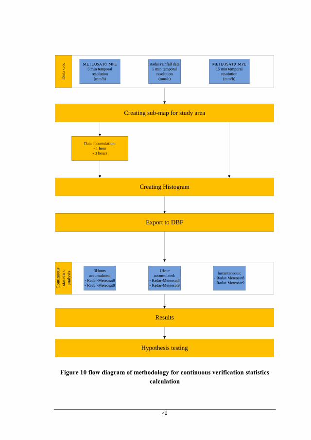
3.2.3. Continuous verification statistics
After pre-processing and processing steps the next step toward calculating
continuous verification statistics is exporting image values as DBF file for
instantaneous maps as well as aggregated maps. For this reason two more command
lines have been added to the scripts, one for creating histogram and the second for
c
.
(mm/h)
40
exporting histogram values as DBF file. Then continuous verification statistics for
assessing errors in magnitude of precipitation calculated. The automation procedure
applied for calculating continuous verification statistics from hundreds of DBF files
which have been achieved from previous step. Appendix D shows related codes in
Visual Basic programming language. Figure 10 illustrates the flow diagram of
methodology for continuous verification statistics calculation.

41
METEOSAT8_MPE
5 min temporal
resolution
(mm/h)
METEOSAT9_MPE
15 min temporal
resolution
(mm/h)
Radar rainfall data
5 min temporal
resolution
(mm/h)
Creating sub-map for study area
Data accumulation:
- 1 hour
- 3 hours
Reclassification to “Rain” and “ No Rain”
3Hours
accumulated:
- Radar-Meteosat8
- Radar-Meteosat9
1Hour
accumulated:
- Radar-Meteosat8
- Radar-Meteosat9
Instantaneous:
- Radar-Meteosat8
- Radar-Meteosat9
- Radar-Meteosat8
- Radar-Meteosat9
Cro
ss t
able
Dat
a se
ts
Cat
ego
rica
l
stat
isti
cs
anal
ysi
s
- Radar-Meteosat8
- Radar-Meteosat9
- Radar-Meteosat8
- Radar-Meteosat9
Results
Hypothesis testing
Figure 9 flow diagram of methodology for categorical verification statistics
calculation
42
METEOSAT8_MPE
5 min temporal
resolution
(mm/h)
METEOSAT9_MPE
15 min temporal
resolution
(mm/h)
Radar rainfall data
5 min temporal
resolution
(mm/h)
Creating sub-map for study area
Data accumulation:
- 1 hour
- 3 hours
Creating Histogram
3Hours
accumulated:
- Radar-Meteosat8
- Radar-Meteosat9
Dat
a se
ts
Co
nti
nu
ou
s
stat
isti
cs
anal
ysi
s 1Hour
accumulated:
- Radar-Meteosat8
- Radar-Meteosat9
Instantaneous:
- Radar-Meteosat8
- Radar-Meteosat9
Results
Hypothesis testing
Export to DBF
Figure 10 flow diagram of methodology for continuous verification statistics
calculation

43
4. Results
According to the KNMI report (figure 11), two main rainfall events have been
selected for comparing estimated rainfall from METEOSAT 8 and METEOSAT 9
with ground radar observation. The first event is 14 to 17 of May 2009 and the
second event 25 to 27 of May 2009. The statistical analysis carried out based on
three temporal resolutions level, instantaneous, 1 hour accumulated and 3 hours
accumulated rainfall.
Figure 11 reported rainfall for May 2009 (source: http://www.knmi.nl )
4.1. The first event
DATE and Time: 20090514, 19:00 UTC to 20090517, 23:45 UTC
The Cloud Analysis Image (CLAI) during this event shows high level clouds
(Cirrus) as well as mid level clouds (Nimbostratus) especially over the Netherlands

44
(e.g. figure 12), other colours refer to land cover, water bodies. The KNMI reported
heavy rain with flooding in this period.
Figure 12 the cloud analysis image for the first event
45
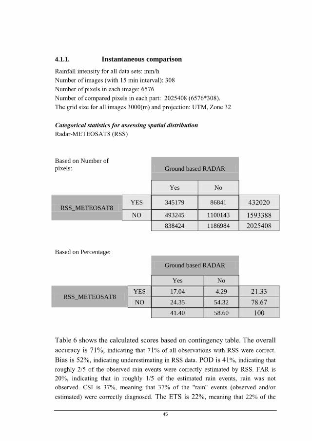
4.1.1. Instantaneous comparison
Rainfall intensity for all data sets: mm/h
Number of images (with 15 min interval): 308
Number of pixels in each image: 6576
Number of compared pixels in each part: 2025408 (6576*308).
The grid size for all images 3000(m) and projection: UTM, Zone 32
Categorical statistics for assessing spatial distribution
Radar-METEOSAT8 (RSS)
Based on Number of
pixels:
Ground based RADAR
Yes No
RSS_METEOSAT8 YES 345179 86841 432020
NO 493245 1100143 1593388
838424 1186984 2025408
Based on Percentage:
Ground based RADAR
Yes No
RSS_METEOSAT8 YES 17.04 4.29 21.33
NO 24.35 54.32 78.67
41.40 58.60 100
Table 6 shows the calculated scores based on contingency table. The overall
accuracy is 71%, indicating that 71% of all observations with RSS were correct.
Bias is 52%, indicating underestimating in RSS data. POD is 41%, indicating that
roughly 2/5 of the observed rain events were correctly estimated by RSS. FAR is
20%, indicating that in roughly 1/5 of the estimated rain events, rain was not
observed. CSI is 37%, meaning that 37% of the "rain" events (observed and/or
estimated) were correctly diagnosed. The ETS is 22%, meaning that 22% of the

46
"rain" events (observed and/or estimated) were correctly diagnosed. The ETS
adjusted for hits associated with random chance.
Table 6 calculated categorical statistics scores between METEOSAT8_RSS and
ground based radar (Event1, instantaneous)
Probability of
Detection(POD)
H/(H+M) 0.41
False Alarm
Ratio (FAR)
F/H+F 0.20
Critical Success
Index (CSI)
H/(H+M+F) 0.37
Accuracy (H+R)/Total N 0.71
Bias (H+F)/(H+M) 0.52
ETS (H- Hrand)/(H+M+F-
Hrand) 0.22
Where H are the correct hits, M are the missed precipitation events, F are the false
precipitation alarms, R the correct rejections and N total number of pixels.
Radar-METEOSAT9
Based on Number of
pixels:
Ground based RADAR
Yes No
METEOSAT9 YES 381565 76178 457743
NO 456859 1110806 1567665
838424 1186984 2025408

47
Based on Percentage:
Ground based RADAR
Yes No
METEOSAT9 YES 18.84 3.76 22.60
NO 22.56 54.84 77.48
41.40 58.60 100
Table 7 shows the calculated scores based on contingency table. The overall
accuracy is 74%, indicating that 74% of all observations with RSS were correct.
Bias is 55%, indicating underestimating in RSS data. POD is 46%, indicating that
almost 1/2 of the observed rain events were correctly estimated by RSS. FAR is
17%, indicating that in roughly 1/5 of the estimated rain events, rain was not
observed. CSI is 42%, meaning that 42% of the "rain" events (observed and/or
estimated) were correctly diagnosed. The ETS is 27%, meaning that 27% of the
"rain" events (observed and/or estimated) were correctly diagnosed. The ETS
adjusted for hits associated with random chance.
Table 7 calculated categorical statistics scores between METEOSA9 and
ground based radar (Event1, instantaneous)
Probability of
Detection(POD)
H/(H+M) 0.46
False Alarm
Ratio (FAR)
F/H+F 0.17
Critical Success
Index (CSI)
H/(H+M+F) 0.42
Accuracy (H+R)/Total N 0.74
Bias (H+F)/(H+M) 0.55
ETS (H- Hrand)/(H+M+F-
Hrand) 0.27

48
Continuous statistics to measure how estimated values by METEOSAT MPE
products differ from the values of ground based radar
Figure 13 shows the comparison between mean rainfall values. These values have
calculated based on weighted rainfall values our whole image. The range of this
value is 0 to 0.7 (mm/h), 0 to 1.48(mm/h), 0 to 2(mm/h) respectively for radar,
METEOSAT 8 and METEOSAT 9.
Figure 13 mean rainfall values (Event1, instantaneous)
The mean error (ME) values shows the differences between estimated and
observed values. The perfect value for ME is zero. Figure 14 illustrates the ME
values for MPE from METEOSAT9 and METEOSAT8. The range of this value is –
0.45 to 0.75(mm/h), - 0.20 to 1.5(mm/h) for METEOSAT8 and METEOSAT9
respectively.
Figure 14 Mean Error (ME) values (Event1, instantaneous)

49
The mean absolute error (MAE) measures the average of the absolute difference
(i.e., negative differences are changed to positive) between the estimates and
observations. Figure 15 shows the MAE values between estimated MPE (from
METEOSAT9 and METEOSAT8) and ground based radar data. The range of this
value is 0 to 0.75(mm/h), 0 to 1.5(mm/h) respectively for METEOSAT 8 and
METEOSAT 9.
Figure 15 Mean Absolute Error values (Event1, instantaneous)
The Root Mean Square Error (RMSE) similar to MAE measures the average error
magnitude but gives greater weight to the larger errors because the differences are
squared before summing. Figure 16 shows the RMSE values between estimated
MPE (from METEOSAT9 and METEOSAT8) and ground based radar data. The
range of this value is 0 to 2.2(mm/h) for METEOSAT 8 and METEOSAT 9.
Figure 16 Root Mean Square Error (RMSE) values (Event1, instantaneous)

50
4.1.2. One hour accumulated rainfall comparison
The rainfall intensity in ground based radar data, METEOSAT8 and METEOSAT9
MPE products are based on mm/h with different temporal resolutions. For one hour
accumulated comparison, in METEOSAT8 and ground based radar data cases with 5
min temporal resolution, 12 images added together then divided by 12 to produce 1
hour accumulated rainfall images. In METEOSAT 9 cases, with 15 min temporal
resolution, 4 images added together then divided by 4 to produce 1 hour
accumulated rainfall images.
Rainfall intensity for all data sets: mm/h
Number of images (with 1 hour interval): 76
Number of pixels in each image: 6576
Number of compared pixels in each part: 499776 (6576*76).
The grid size for all images 3000(m) and projection: UTM, Zone 32
Categorical statistics for assessing spatial distribution
Radar-METEOSAT8 (RSS)
Based on Number of
pixels:
Ground based RADAR
Yes No
RSS_METEOSAT8 YES 123409 23640 147049
NO 120660 232067 352727
244069 255707 499776
Based on Percentage:
Ground based RADAR
Yes No
RSS_METEOSAT8 YES 24.69 4.73 29.42
NO 24.14 46.43 70.58
48.84 51.16 100

51
Table 8 shows the calculated scores based on contingency table. The overall
accuracy is 71%, indicating that 71% of all observations with RSS were correct.
Bias is 60%, indicating underestimating in RSS data. POD is 51%, indicating that
roughly 1/2 of the observed rain events were correctly estimated by RSS. FAR is
16%, indicating that in roughly 1/6 of the estimated rain events, rain was not
observed. CSI is 46%, meaning that 46% of the "rain" events (observed and/or
estimated) were correctly diagnosed. The ETS is 26%, meaning that 26% of the
"rain" events (observed and/or estimated) were correctly diagnosed. The ETS
adjusted for hits associated with random chance.
Table 8 calculated categorical statistics scores between METEOSAT8_RSS and
ground based radar (Event1, 1 Hour accumulated)
Probability of
Detection(POD)
H/(H+M) 0.51
False Alarm
Ratio (FAR)
F/H+F 0.16
Critical Success
Index (CSI)
H/(H+M+F) 0.46
Accuracy (H+R)/Total N 0.71
Bias (H+F)/(H+M) 0.60
ETS (H- Hrand)/(H+M+F-
Hrand) 0.26

52
Radar-METEOSAT9
Based on Number of
pixels:
Ground based RADAR
Yes No
METEOSAT9 YES 129439 18994 148433
NO 114630 236713 351343
244069 255707 499776
Based on Percentage:
Ground based RADAR
Yes No
METEOSAT9 YES 25.90 3.80 29.70
NO 22.94 47.36 70.30
48.84 51.16 100
Table 9 shows the calculated scores based on contingency table. The overall
accuracy is 73%, indicating that 73% of all observations with RSS were correct.
Bias is 61%, indicating underestimating in RSS data. POD is 53%, indicating that
almost 1/2 of the observed rain events were correctly estimated by RSS. FAR is
13%, indicating that in roughly 1/7 of the estimated rain events, rain was not
observed. CSI is 49%, meaning that 49% of the "rain" events (observed and/or
estimated) were correctly diagnosed. The ETS is 30%, meaning that 30% of the
"rain" events (observed and/or estimated) were correctly diagnosed. The ETS
adjusted for hits associated with random chance.

53
Table 9 calculated categorical statistics scores between METEOSA9 and
ground based radar (Event1, 1 Hour accumulated)
Probability of
Detection(POD)
H/(H+M) 0.53
False Alarm
Ratio (FAR)
F/H+F 0.13
Critical Success
Index (CSI)
H/(H+M+F) 0.49
Accuracy (H+R)/Total N 0.73
Bias (H+F)/(H+M) 0.61
ETS (H- Hrand)/(H+M+F-
Hrand) 0.30
Continuous statistics to measure how estimated values by METEOSAT MPE
products differ from the values of ground based radar
Figure 17shows the comparison between mean rainfall values. These values have
calculated based on weighted rainfall values our whole image. The range of this
value is 0 to 0.7 (mm/h), 0 to 1.48(mm/h), 0 to 1.9(mm/h) respectively for radar,
METEOSAT8 and METEOSAT9.
Figure 17 mean rainfall values (Event1, 1Hour accumulated)

54
Figure 18 illustrates the ME values for MPE from METEOSAT9 and
METEOSAT8. The range of this value is – 0.30 to 0.8(mm/h), - 0.20 to 1.42(mm/h)
respectively for METEOSAT 8 and METEOSAT 9.
Figure 18 Mean Error (ME) values (Event1, 1Hour accumulated)
Figure 19 shows the MAE values between estimated MPE (from METEOSAT9 and
METEOSAT8) and ground based radar data. The range of this value is 0 to
0.8(mm/h), 0 to 1.42(mm/h) respectively for METEOSAT 8 and METEOSAT 9.
Figure 19 Mean Absolute Error values (Event1, 1Hour accumulated)

55
Figure 20 shows the RMSE values between estimated MPE (from METEOSAT9
and METEOSAT8) and ground based radar data. The range of this value is 0 to
1.4(mm/h), 0 to 1.8(mm/h) respectively for METEOSAT 8 and METEOSAT 9.
Figure 20 Root Mean Square Error (RMSE) values (Event1, 1Hour
accumulated)
4.1.3. Three hours accumulated rainfall comparison
The rainfall intensity in ground based radar data, METEOSAT8 and METEOSAT9
MPE products are based on mm/h with different temporal resolutions. For three
hours accumulated comparison, in METEOSAT8 and ground based radar data cases
with 5 min temporal resolution, 36 images added together then divided by 12 to
produce three hours accumulated rainfall images (mm/3h). In METEOSAT 9 cases,
with 15 min temporal resolution, 12 images added together then divided by 4 to
produce three hours accumulated rainfall images (mm/3h).
Rainfall intensity for all data sets: mm/3h
Number of images (with 3 hours interval): 25
Number of pixels in each image: 6576
Number of compared pixels in each part: 164400 (6576*25).
The grid size for all images 3000(m) and projection: UTM, Zone 32
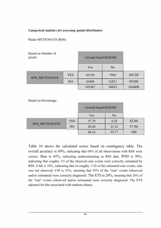
56
Categorical statistics for assessing spatial distribution
Radar-METEOSAT8 (RSS)
Based on Number of
pixels:
Ground based RADAR
Yes No
RSS_METEOSAT8 YES 62118 7002 69120
NO 43469 51811 95280
105587 58813 164400
Based on Percentage:
Ground based RADAR
Yes No
RSS_METEOSAT8 YES 37.78 4.26 42.04
NO 26.44 31.52 57.96
64.23 35.77 100
Table 10 shows the calculated scores based on contingency table. The
overall accuracy is 69%, indicating that 69% of all observations with RSS were
correct. Bias is 65%, indicating underestimating in RSS data. POD is 59%,
indicating that roughly 3/5 of the observed rain events were correctly estimated by
RSS. FAR is 10%, indicating that in roughly 1/10 of the estimated rain events, rain
was not observed. CSI is 55%, meaning that 55% of the "rain" events (observed
and/or estimated) were correctly diagnosed. The ETS is 26%, meaning that 26% of
the "rain" events (observed and/or estimated) were correctly diagnosed. The ETS
adjusted for hits associated with random chance.

57
Table 10 calculated categorical statistics scores between METEOSAT8_RSS
and ground based radar (Event1, 3 Hours accumulated)
Probability of
Detection(POD)
H/(H+M) 0.59
False Alarm
Ratio (FAR)
F/H+F 0.10
Critical Success
Index (CSI)
H/(H+M+F) 0.55
Accuracy (H+R)/Total N 0.69
Bias (H+F)/(H+M) 0.65
ETS (H- Hrand)/(H+M+F-
Hrand) 0.26
Radar-METEOSAT9
Based on Number of
pixels:
Ground based RADAR
Yes No
METEOSAT9 YES 58462 4678 63140
NO 44708 56552 101260
103170 61230 164400

58
Based on Percentage:
Ground based RADAR
Yes No
METEOSAT9 YES 35.56 2.85 38.41
NO 27.19 34.40 61.59
62.76 37.24 100
Table 11 shows the calculated scores based on contingency table. The
overall accuracy is 70%, indicating that 70% of all observations with RSS were
correct. Bias is 61%, indicating underestimating in RSS data. POD is 57%,
indicating that almost 3/5 of the observed rain events were correctly estimated by
RSS. FAR is 7%, indicating that in roughly 1/14 of the estimated rain events, rain
was not observed. CSI is 54%, meaning that 54% of the "rain" events (observed
and/or estimated) were correctly diagnosed. The ETS is 28%, meaning that 28% of
the "rain" events (observed and/or estimated) were correctly diagnosed. The ETS
adjusted for hits associated with random chance.
Table 11 calculated categorical statistics scores between METEOSA9 and
ground based radar (Event1, 3Hours accumulated)
Probability of
Detection(POD)
H/(H+M) 0.57
False Alarm
Ratio (FAR)
F/H+F 0.07
Critical Success
Index (CSI)
H/(H+M+F) 0.54
Accuracy (H+R)/Total N 0.70
Bias (H+F)/(H+M) 0.61
ETS (H- Hrand)/(H+M+F-
Hrand) 0.28
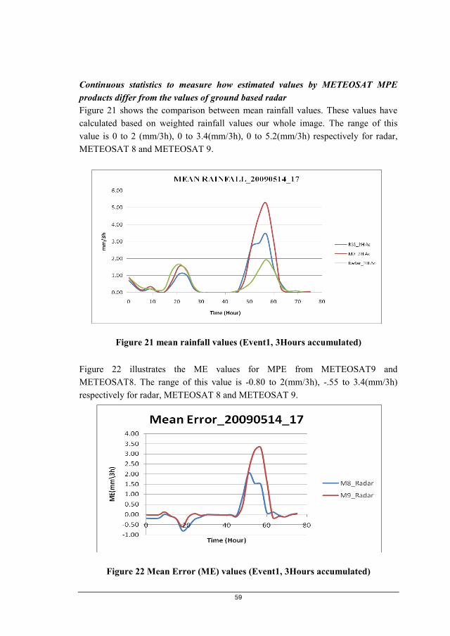
59
Continuous statistics to measure how estimated values by METEOSAT MPE
products differ from the values of ground based radar
Figure 21 shows the comparison between mean rainfall values. These values have
calculated based on weighted rainfall values our whole image. The range of this
value is 0 to 2 (mm/3h), 0 to 3.4(mm/3h), 0 to 5.2(mm/3h) respectively for radar,
METEOSAT 8 and METEOSAT 9.
Figure 21 mean rainfall values (Event1, 3Hours accumulated)
Figure 22 illustrates the ME values for MPE from METEOSAT9 and
METEOSAT8. The range of this value is -0.80 to 2(mm/3h), -.55 to 3.4(mm/3h)
respectively for radar, METEOSAT 8 and METEOSAT 9.
Figure 22 Mean Error (ME) values (Event1, 3Hours accumulated)

60
Figure 23 shows the MAE values between estimated MPE (from METEOSAT9 and
METEOSAT8) and ground based radar data. The range of this value is 0 to
2(mm/3h), 0 to 3.4(mm/3h) respectively for radar, METEOSAT 8 and METEOSAT
9.
Figure 23 Mean Absolute Error values (Event1, 3Hours accumulated)
Figure 24 shows the RMSE values between estimated MPE (from METEOSAT9
and METEOSAT8) and ground based radar data. The range of this value is 0 to
3.5(mm/3h), 0 to 4.5 (mm/3h) respectively for radar, METEOSAT 8 and
METEOSAT 9.
Figure 24 Root Mean Square Error (RMSE) values (Event1, 3Hours
accumulated)
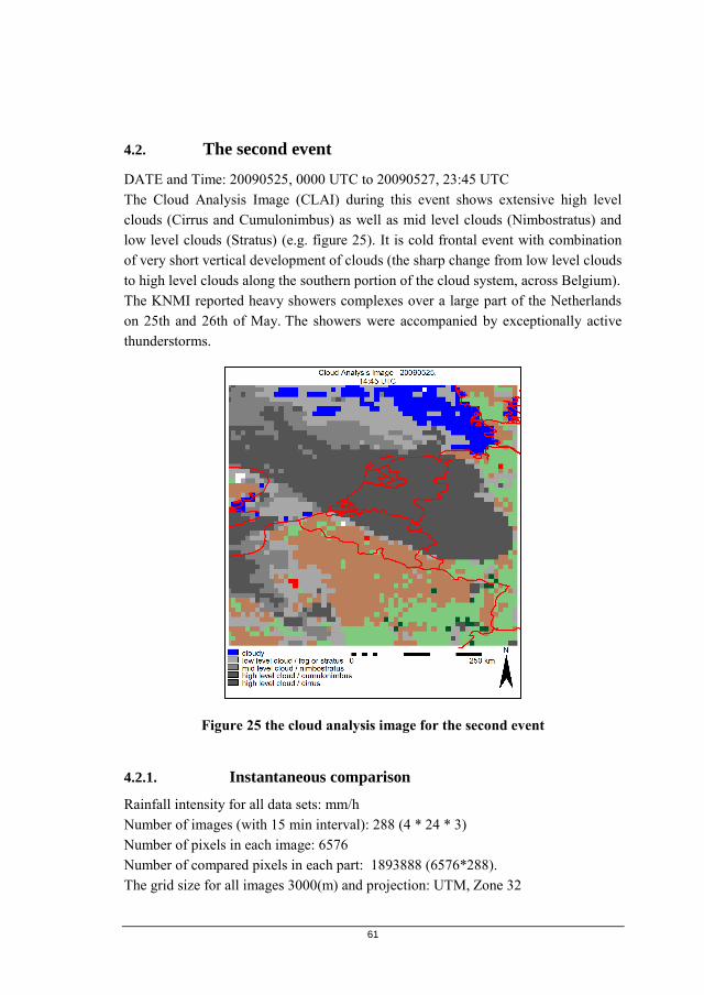
61
4.2. The second event
DATE and Time: 20090525, 0000 UTC to 20090527, 23:45 UTC
The Cloud Analysis Image (CLAI) during this event shows extensive high level
clouds (Cirrus and Cumulonimbus) as well as mid level clouds (Nimbostratus) and
low level clouds (Stratus) (e.g. figure 25). It is cold frontal event with combination
of very short vertical development of clouds (the sharp change from low level clouds
to high level clouds along the southern portion of the cloud system, across Belgium).
The KNMI reported heavy showers complexes over a large part of the Netherlands
on 25th and 26th of May. The showers were accompanied by exceptionally active
thunderstorms.
Figure 25 the cloud analysis image for the second event
4.2.1. Instantaneous comparison
Rainfall intensity for all data sets: mm/h
Number of images (with 15 min interval): 288 (4 * 24 * 3)
Number of pixels in each image: 6576
Number of compared pixels in each part: 1893888 (6576*288).
The grid size for all images 3000(m) and projection: UTM, Zone 32

62
Categorical statistics for assessing spatial distribution
Radar-METEOSAT8 (RSS)
Based on Number of
pixels:
Ground based RADAR
Yes No
RSS_METEOSAT8 YES 206425 108147 314572
NO 413321 1165995 1579316
619746 1274142 1893888
Based on Percentage:
Ground based RADAR
Yes No
RSS_METEOSAT8 YES 10.90 5.71 16.61
NO 21.82 61.57 83.39
32.72 67.28 100
Table 12 shows the calculated scores based on contingency table. The
overall accuracy is 72%, indicating that 72% of all observations with RSS were
correct. Bias is 51%, indicating underestimating in RSS data. POD is 33%,
indicating that roughly 1/3 of the observed rain events were correctly estimated by
RSS. FAR is 34%, indicating that in roughly 1/3 of the estimated rain events, rain
was not observed. CSI is 28%, meaning that 28% of the "rain" events (observed
and/or estimated) were correctly diagnosed. The ETS is 17%, meaning that 17% of
the "rain" events (observed and/or estimated) were correctly diagnosed. The ETS
adjusted for hits associated with random chance.
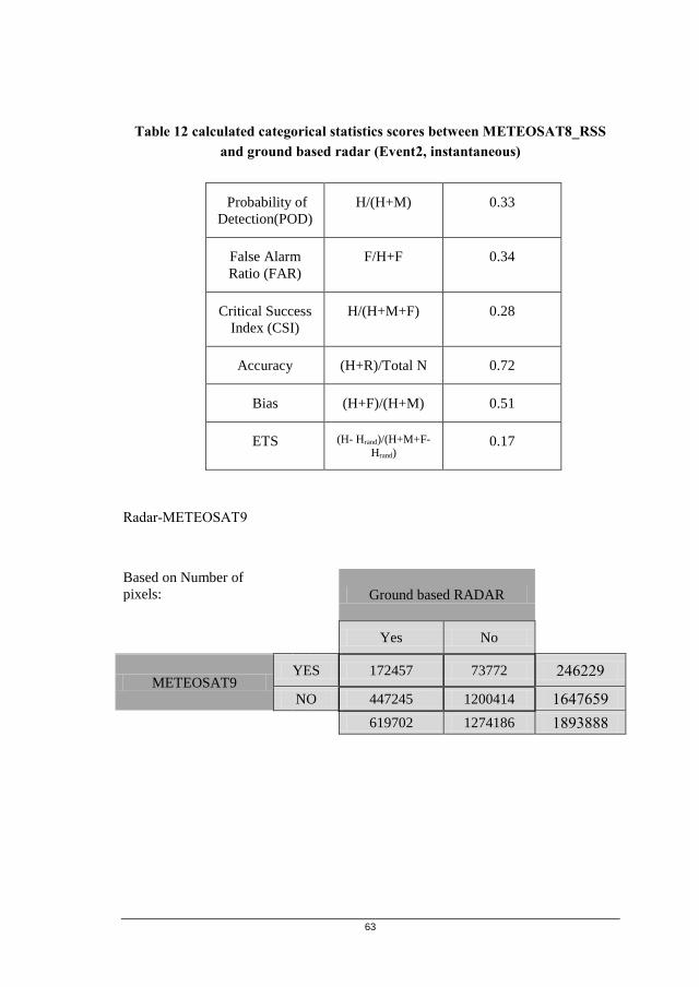
63
Table 12 calculated categorical statistics scores between METEOSAT8_RSS
and ground based radar (Event2, instantaneous)
Probability of
Detection(POD)
H/(H+M) 0.33
False Alarm
Ratio (FAR)
F/H+F 0.34
Critical Success
Index (CSI)
H/(H+M+F) 0.28
Accuracy (H+R)/Total N 0.72
Bias (H+F)/(H+M) 0.51
ETS (H- Hrand)/(H+M+F-
Hrand) 0.17
Radar-METEOSAT9
Based on Number of
pixels:
Ground based RADAR
Yes No
METEOSAT9 YES 172457 73772 246229
NO 447245 1200414 1647659
619702 1274186 1893888

64
Based on Percentage:
Ground based RADAR
Yes No
METEOSAT9 YES 9.11 3.90 13
NO 23.62 63.38 87
32.72 67.28 100
Table 13 shows the calculated scores based on contingency table. The
overall accuracy is 72%, indicating that 72% of all observations with RSS were
correct. Bias is 40%, indicating underestimating in RSS data. POD is 28%,
indicating that almost 1/4 of the observed rain events were correctly estimated by
RSS. FAR is 30%, indicating that in roughly 1/3 of the estimated rain events, rain
was not observed. CSI is 25%, meaning that 25% of the "rain" events (observed
and/or estimated) were correctly diagnosed. The ETS is 15%, meaning that 15% of
the "rain" events (observed and/or estimated) were correctly diagnosed. The ETS
adjusted for hits associated with random chance.
Table 13 calculated categorical statistics scores between METEOSA9 and
ground based radar (Event2, instantaneous)
Probability of
Detection(POD)
H/(H+M) 0.28
False Alarm
Ratio (FAR)
F/H+F 0.30
Critical Success
Index (CSI)
H/(H+M+F) 0.25
Accuracy (H+R)/Total N 0.72
Bias (H+F)/(H+M) 0.40
ETS (H- Hrand)/(H+M+F-
Hrand) 0.15

65
Continuous statistics to measure how estimated values by METEOSAT MPE
products differ from the values of ground based radar.
Figure 26 shows the comparison between mean rainfall values. These values have
calculated based on weighted rainfall values our whole image. The range of this
value is 0 to 1.8 (mm/h), 0 to 11(mm/h), 0 to 10.8(mm/h) respectively for radar,
METEOSAT 8 and METEOSAT 9.
Figure 26 mean rainfall values (Event2, instantaneous)
Figure 27 illustrates the ME values for MPE from METEOSAT9 and
METEOSAT8. The range of this value is -0.2 to 10 (mm/h), -0.2 to 9.9(mm/h)
respectively for METEOSAT 8 and METEOSAT 9.
Figure 27 Mean Error (ME) values (Event2, instantaneous)

66
Figure 28 shows the MAE values between estimated MPE (from METEOSAT9 and
METEOSAT8) and ground based radar data. The range of this value is 0 to 10
(mm/h), -0.2 to 9.9(mm/h) respectively for METEOSAT 8 and METEOSAT 9.
Figure 28 Mean Absolute Error (MAE) values (Event2, instantaneous)
Figure 29 shows the RMSE values between estimated MPE (from METEOSAT9
and METEOSAT8) and ground based radar data. The range of this value is 0 to 12.5
(mm/h), 0 to 13(mm/h) respectively for METEOSAT 8 and METEOSAT 9.
Figure 29 Root Mean Square Error (RMSE) values (Event2, instantaneous)

67
4.2.2. One hour accumulated rainfall comparison
Rainfall intensity for all data sets: mm/h
Number of images (with 1 hour interval): 72
Number of pixels in each image: 6576
Number of compared pixels in each part: 473472 (6576*72).
The grid size for all images 3000(m) and projection: UTM, Zone 32
Categorical statistics for assessing spatial distribution
Radar-METEOSAT8 (RSS)
Based on Number of
pixels:
Ground based RADAR
Yes No
RSS_METEOSAT8 YES 63933 29160 93093
NO 121417 258962 380379
185350 288122 473472
Based on Percentage:
Ground based RADAR
Yes No
RSS_METEOSAT8 YES 13.50 6.16 19.66
NO 25.64 54.69 80.34
39.15 60.85 100
Table 14 shows the calculated scores based on contingency table. The
overall accuracy is 68%, indicating that 68% of all observations with RSS were
correct. Bias is 50%, indicating underestimating in RSS data. POD is 34%,
indicating that roughly 1/3 of the observed rain events were correctly estimated by
RSS. FAR is 31%, indicating that in roughly 1/3 of the estimated rain events, rain
was not observed. CSI is 30%, meaning that 30% of the "rain" events (observed
and/or estimated) were correctly diagnosed. The ETS is 15%, meaning that 15% of

68
the "rain" events (observed and/or estimated) were correctly diagnosed. The ETS
adjusted for hits associated with random chance.
Table 14 calculated categorical statistics scores between METEOSAT8_RSS
and ground based radar (Event2, 1 Hour accumulated)
Probability of
Detection(POD)
H/(H+M) 0.34
False Alarm
Ratio (FAR)
F/H+F 0.31
Critical Success
Index (CSI)
H/(H+M+F) 0.30
Accuracy (H+R)/Total N 0.68
Bias (H+F)/(H+M) 0.50
ETS (H- Hrand)/(H+M+F-
Hrand) 0.15
Radar-METEOSAT9
Based on Number of
pixels:
Ground based RADAR
Yes No
METEOSAT9 YES 57539 21268 78807
NO 127811 266854 394665
185350 288122 473472

69
Based on Percentage:
Ground based RADAR
Yes No
METEOSAT9 YES 12.15 4.49 16.64
NO 26.99 56.36 83.36
39.15 60.85 100
Table 15 shows the calculated scores based on contingency table. The
overall accuracy is 69%, indicating that 69% of all observations with RSS were
correct. Bias is 43%, indicating underestimating in RSS data. POD is 31%,
indicating that almost 1/3 of the observed rain events were correctly estimated by
RSS. FAR is 27%, indicating that in roughly 1/3 of the estimated rain events, rain
was not observed. CSI is 28%, meaning that 28% of the "rain" events (observed
and/or estimated) were correctly diagnosed. The ETS is 15%, meaning that 15% of
the "rain" events (observed and/or estimated) were correctly diagnosed. The ETS
adjusted for hits associated with random chance.
Table 15 calculated categorical statistics scores between METEOSA9 and
ground based radar (Event2, 1 Hour accumulated)
Probability of
Detection(POD)
H/(H+M) 0.31
False Alarm
Ratio (FAR)
F/H+F 0.27
Critical Success
Index (CSI)
H/(H+M+F) 0.28
Accuracy (H+R)/Total N 0.69
Bias (H+F)/(H+M) 0.43
ETS (H- Hrand)/(H+M+F-
Hrand) 0.15

70
Continuous statistics to measure how estimated values by METEOSAT MPE
products differ from the values of ground based radar
Figure 30 shows the comparison between mean rainfall values. These values have
calculated based on weighted rainfall values our whole image. The range of this
value is 0 to 1.8 (mm/h), 0 to 11(mm/h), 0 to 10 (mm/h) respectively for radar,
METEOSAT 8 and METEOSAT 9.
Figure 30 mean rainfall values (Event2, 1 Hour accumulated)
Figure 31 illustrates the ME values for MPE from METEOSAT9 and
METEOSAT8. The range of this value is -0.2 to 10 (mm/h), -0.2 to 9.50(mm/h)
respectively for METEOSAT 8 and METEOSAT 9.
Figure 31 Mean Error (ME) values (Event2, 1 Hour accumulated)

71
Figure 32 shows the MAE values between estimated MPE (from METEOSAT9 and
METEOSAT8) and ground based radar data. The range of this value is 0 to 10
(mm/h), 0 to 9.50(mm/h) respectively for METEOSAT 8 and METEOSAT 9.
.
Figure 32 Mean Absolute Error (MAE) values (Event2, 1 Hour accumulated)
Figure 33 shows the RMSE values between estimated MPE (from METEOSAT9
and METEOSAT8) and ground based radar data. The range of this value is 0 to 11.8
(mm/h), 0 to 11.7(mm/h) respectively for METEOSAT 8 and METEOSAT 9.
Figure 33 Root Mean Square Error (RMSE) values (Event2, 1 Hour
accumulated)
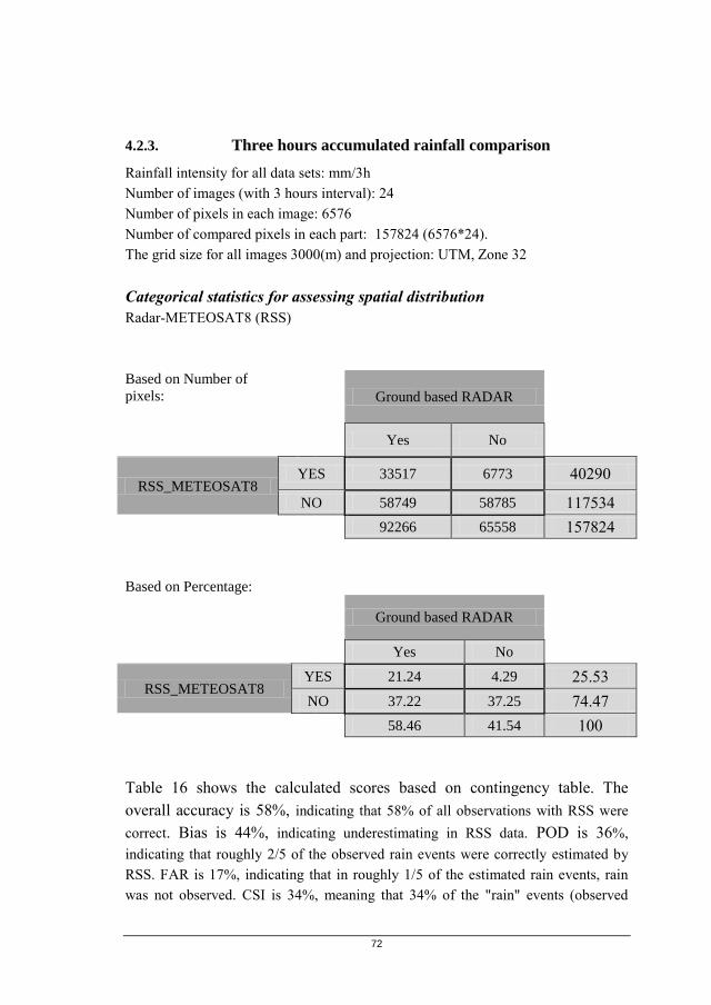
72
4.2.3. Three hours accumulated rainfall comparison
Rainfall intensity for all data sets: mm/3h
Number of images (with 3 hours interval): 24
Number of pixels in each image: 6576
Number of compared pixels in each part: 157824 (6576*24).
The grid size for all images 3000(m) and projection: UTM, Zone 32
Categorical statistics for assessing spatial distribution
Radar-METEOSAT8 (RSS)
Based on Number of
pixels:
Ground based RADAR
Yes No
RSS_METEOSAT8 YES 33517 6773 40290
NO 58749 58785 117534
92266 65558 157824
Based on Percentage:
Ground based RADAR
Yes No
RSS_METEOSAT8 YES 21.24 4.29 25.53
NO 37.22 37.25 74.47
58.46 41.54 100
Table 16 shows the calculated scores based on contingency table. The
overall accuracy is 58%, indicating that 58% of all observations with RSS were
correct. Bias is 44%, indicating underestimating in RSS data. POD is 36%,
indicating that roughly 2/5 of the observed rain events were correctly estimated by
RSS. FAR is 17%, indicating that in roughly 1/5 of the estimated rain events, rain
was not observed. CSI is 34%, meaning that 34% of the "rain" events (observed
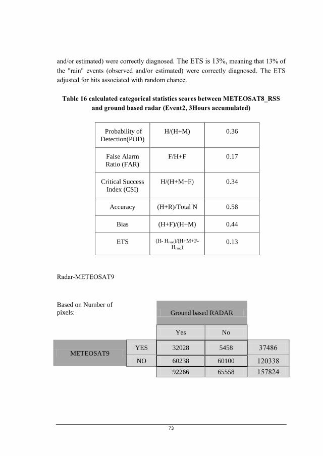
73
and/or estimated) were correctly diagnosed. The ETS is 13%, meaning that 13% of
the "rain" events (observed and/or estimated) were correctly diagnosed. The ETS
adjusted for hits associated with random chance.
Table 16 calculated categorical statistics scores between METEOSAT8_RSS
and ground based radar (Event2, 3Hours accumulated)
Probability of
Detection(POD)
H/(H+M) 0.36
False Alarm
Ratio (FAR)
F/H+F 0.17
Critical Success
Index (CSI)
H/(H+M+F) 0.34
Accuracy (H+R)/Total N 0.58
Bias (H+F)/(H+M) 0.44
ETS (H- Hrand)/(H+M+F-
Hrand) 0.13
Radar-METEOSAT9
Based on Number of
pixels:
Ground based RADAR
Yes No
METEOSAT9 YES 32028 5458 37486
NO 60238 60100 120338
92266 65558 157824

74
Based on Percentage:
Ground based RADAR
Yes No
METEOSAT9 YES 20.29 3.49 23.75
NO 38.17 38.08 76.25
58.46 41.54 100
Table 17 shows the calculated scores based on contingency table. The
overall accuracy is 58%, indicating that 58% of all observations with RSS were
correct. Bias is 41%, indicating underestimating in RSS data. POD is 35%,
indicating that almost 1/3 of the observed rain events were correctly estimated by
RSS. FAR is 15%, indicating that in roughly 1/7 of the estimated rain events, rain
was not observed. CSI is 33%, meaning that 33% of the "rain" events (observed
and/or estimated) were correctly diagnosed. The ETS is 13%, meaning that 13% of
the "rain" events (observed and/or estimated) were correctly diagnosed. The ETS
adjusted for hits associated with random chance.
Table 17 calculated categorical statistics scores between METEOSA9 and
ground based radar (Event2, 3Hours accumulated)
Probability of
Detection(POD)
H/(H+M) 0.35
False Alarm
Ratio (FAR)
F/H+F 0.15
Critical Success
Index (CSI)
H/(H+M+F) 0.33
Accuracy (H+R)/Total N 0.58
Bias (H+F)/(H+M) 0.41
ETS (H- Hrand)/(H+M+F-
Hrand) 0.13

75
Continuous statistics to measure how estimated values by METEOSAT MPE
products differ from the values of ground based radar
Figure 34 shows the comparison between mean rainfall values. These values have
calculated based on weighted rainfall values our whole image. The range of this
value is 0 to 3.5 (mm/3h), 0 to 30(mm/3h), 0 to 27 (mm/3h) respectively for radar,
METEOSAT 8 and METEOSAT 9.
Figure 34 mean rainfall values (Event2, 3 Hours accumulated)
Figure 35 illustrates the ME values for MPE from METEOSAT9 and
METEOSAT8. The range of this value is -0.2 to 25.2 (mm/3h), -0.2 to 24(mm/3h)
respectively for METEOSAT 8 and METEOSAT 9.
Figure 35 Mean Error (ME) values (Event2, 3 Hours accumulated)

76
Figure 36 shows the MAE values between estimated MPE (from METEOSAT9 and
METEOSAT8) and ground based radar data. The range of this value is 0 to 25.2
(mm/3h), 0 to 24(mm/3h) respectively for METEOSAT 8 and METEOSAT 9.
Figure 36 Mean Absolute Error (MAE) values (Event2, 3Hours accumulated)
Figure 37 shows the RMSE values between estimated MPE (from METEOSAT9
and METEOSAT8) and ground based radar data. The range of this value is 0 to 29.5
(mm/3h), 0 to 26(mm/3h) respectively for METEOSAT 8 and METEOSAT 9.
Figure 37 Root Mean Square Error (RMSE) values (Event2, 3Hours
accumulated)

77
5. Discussion
5.1. Spatial distribution assessment
The summery of spatial distribution assessment results presented in table 18, table
19, and table 20, for instantaneous, one hour accumulated and three hours
accumulated time intervals respectively.
The POD is increasing gradually from 0.28 for METEOSAT9, event2, instantaneous
to 0.59 for METEOSAT 8, event1, three hours accumulated. The highest probability
of detection is 0.59, for METEOSAT 8, indicating that roughly 3/5 of the observed
rain events were correctly estimated by METOSAT 8 for event 1 with three hours
accumulated data sets. The POD for METEOSAT9 in event1 with 15 min and one
hour temporal resolution is higher than METEOSAT 8. However, METEOSAT8
yields higher POD in all time intervals for the second event. This shows the number
of detected hits by METEOSAT8 for the second event is more than METEOSAT9.
This score is sensitive to hits and insensitive to false alarms.
The FAR for both satellites is decreasing by increasing time intervals from 15 min to
3 hours accumulated. The minimum false alarm ratio is 0.07, for METEOSAT 9,
event1, three hours accumulated. This value indicates that 7% of diagnosed events
that were actually did not occur. The FAR in all events and time intervals for
METEOSAT9 is lower than METEOSAT8. This shows that METEOSAT8 has wet
bias. FAR is sensitive to false alarms and insensitive to hits. Thus FAR and POD
should always be used together. Because good or even perfect value in either case
individually are easily obtained. For example if an algorithm has wet bias such that
it always detects rain everywhere all the time, POD will be perfect (“1”). However,
the FAR will also be close to the worse score (“1”) (Levizzani et al. 2007).
The CSI is rising gradually by increasing accumulation time from 15min to three
hours accumulated. The maximum resulted CSI is 0.55, for METEOSAT8, first
event, three hours accumulated, which is almost equal to the value, resulted from
METEOSAT9. This value shows 55% of the "rain" events (observed and/or
estimated) were correctly diagnosed. The CSI for METEOSAT9 in event1 with 15
min and one hour temporal resolution is higher than METEOSAT 8. However,
METEOSAT8 yields higher CSI in all time intervals for the second event. The CSI
can be thought as accuracy when correct negatives have been removed from
consideration. The CSI is sensitive to hits and it always increases with rain fraction.
Thus, estimations for wetter regions or seasons might appear to have greater skill

78
than dry seasons even though the ability to estimate rain or not-rain has not changed
(biased to samples with higher precipitation frequency). The CSI penalizes both
misses and false alarms.
The overall accuracy values are decreasing by increasing time intervals. These
values are almost the same for both METEOSAT8 and METEOSAT9. The range of
this score for the first event is 0.69 to 0.74 and the second is 0.58 to 0.72. These
values Indicates 60% to 70% of all observations with METEOSAT9 and
METEOSAT8 were correct. The accuracy value is sensitive to both hits and correct
negative, therefore even if no rain detected it increases with correct negative
fraction.
The bias is increasing gradually by increasing accumulation time from 15min to
three hours accumulated. The range of this score is from 0.40 to 0.65.which shows
underestimation in all cases. For the first event, METEOSAT9 yields better results
for instantaneous and one hour accumulated comparison. However this value for the
METEOSAT8 in the second event (all temporal resolutions) as well as the first event
with three hours accumulated rainfall is higher than METEOSAT9. The best
obtained bias value is 0.65, for METEOSAT 8, second event, three hours
accumulated rainfall. It means the number of estimated pixels with rainfall by
METEOSAT 9 is less than the number of observed pixels by ground based radar.
The ETS value changes trend is almost similar to the CSI. The highest resulted ETS
value is 0.30, for METEOSAT9, first event, one hour accumulated. This value
shows 30% of the "rain" events (observed and/or estimated) were correctly
diagnosed. This score is almost similar to CSI but it is adjusted for hits associated
with random chance. ETS gives a lower score than the CSI.
Table 18 results for categorical statistics analysis (instantaneous)
Statistical
Score
Radar _METEOSAT 9 Radar _METEOSAT 8(RSS)
Event1 Event2 Event1 Event2
POD 0.46 0.28 0.41 0.33
FAR 0.17 0.30 0.20 0.34
CSI 0.42 0.25 0.37 0.28
Accuracy 0.74 0.72 0.71 0.72
Bias 0.55 0.40 0.52 0.51
ETS 0.27 0.15 0.22 0.17

79
Table 19 results for categorical statistical analysis (one hour accumulated)
Statistical
Score
Radar _METEOSAT 9 Radar _METEOSAT 8(RSS)
Event1 Event2 Event1 Event2
POD 0.53 0.31 0.51 0.34
FAR 0.13 0.27 0.16 0.31
CSI 0.49 0.28 0.46 0.30
Accuracy 0.73 0.69 0.71 0.68
Bias 0.61 0.43 0.60 0.50
ETS 0.30 0.15 0.26 0.15
Table 20 results for categorical statistical analysis (three hours accumulated)
Statistical
Score
Radar _METEOSAT 9 Radar _METEOSAT 8(RSS)
Event1 Event2 Event1 Event2
POD 0.57 0.35 0.59 0.36
FAR 0.07 0.15 0.10 0.17
CSI 0.54 0.33 0.55 0.34
Accuracy 0.70 0.58 0.69 0.58
Bias 0.61 0.41 0.65 0.44
ETS 0.28 0.13 0.26 0.13

80
5.2. Assessing errors in magnitude
Regression between mean rainfall values for assessing MPE products form
METEOSAT 9 and METEOSA 8 with α=0.05 (95% confidence level). Tables 21,
22 and 23 show the results for regression analysis for instantaneous, one hour
accumulated and three hours accumulated comparison respectively. The results
indicate the MPE product from both satellites for the first event is strongly
correlated with ground based radar data. However, for the second event MPE
product from both satellites moderately correlated with ground based radar data.
The r² is increasing gradually by increasing accumulation time from 15min to three
hours accumulated.
The regressions are all highly significant, with significance of F values well below
the designated α value of 0.05. The significance of F is a measure of relationship
between the x and y variables and tests the null hypothesis that there is no
relationship between the x and y variables (Moore and McCabe 2002). Therefore, if
the significance of F is much less than α, as in the case of three different temporal
resolutions comparison for two different events, it can be assumed that there is linear
relationship between the variables (ground based radar data and satellite MPE
products).
In all cases the slope of the regressions are highly statistically significant at α=0.05,
where the p-values are 1.51E-127 to 7.46E-06. This means that the slopes of the
lines are all significantly different from zero. On this alone it may be fair to say that
the regression could be used as a predictor of the dependent variable (MPE) for any
value of the independent variable (ground based radar data). However, statistical
significance may not necessarily mean practical importance. Just by looking at the
example scatter graph of the second event, instantaneous comparison, in figure 38,
one can see that the MPE algorithm tends to overestimate. The overestimation by
MPE products in all cases has confirmed by resulted graphs for ME, MAE and
RMSE in chapter 4. As it is clearly stated in chapter 4, the amount of overestimation
by MPE products for the second event is more than the first event. Therefore, it is
fair to say the MPE products have more difficulty in estimating severe events.

81
Figure 38 Scatter graph for MPE products, instantaneous comparison, second
event
The diagonal dotted line in the graph shows the ideal 1:1 relationship between
reference values and estimated values by METEOSAT 8 and METEOSAT 9, and
the black line is the regression of the true relationship. The graph shows over
estimation in METEOSAT 8 and METEOSAT 9 MPE values.
Table 21 Regressions for mean rainfall values in MPE products, instantaneous
comparison, α=0.05
Radar _METEOSAT 9 Radar _METEOSAT 8(RSS)
Event1 Event2 Event1 Event2
Observations (n) 288 308 288 308
Slope coefficient, p-value 7.35, 3.56E-122 1.84, 3.2E-64 7.96, 1.51E-127 1.21, 1.42E-58
Intercept coefficient,
p-value -0.11, 0.047 -0.03, 0.27 -0.16, .004 0.01, 0.50
r² 0.85 0.61 0.87 0.57
Significance F 3.57E-122 3.2E-64 1.51E-127 1.42E-58

82
Table 22 Regressions for mean rainfall values in MPE products, one hour
accumulated, α=0.05
Radar _METEOSAT 9 Radar _METEOSAT 8(RSS)
Event1 Event2 Event1 Event2
Observations (n) 72 77 72 77
Slope coefficient,
p-value 7.60, 6.13E-35 1.84, 9.72E-17 8.23, 2.59E-36 1.20, 3.89E-15
Intercept coefficient,
p-value -0.13, 0.18 -0.03, 0.58 -0.18, .06 0.01, 0.71
r² 0.89 0.60 0.90 0.56
Significance F 6.13E-35 9.72E-17 2.59E-36 3.89E-15
Table 23 Regressions for mean rainfall values in MPE products, three hours
accumulated, α=0.05
Radar _METEOSAT 9 Radar _METEOSAT 8(RSS)
Event1 Event2 Event1 Event2
Observations (n) 24 25 24 25
Slope coefficient, p-value 7.82, 1.79E-14 1.98, 6.61E-07 8.43, 2.61E-15 1.26, 7.46E-06
Intercept coefficient,
p-value -0.50, 0.19 -0.13, 0.59 -0.65, 0.09 0.02, 0.92
r² 0.93 0.67 0.94 0.59
Significance F 1.79E-14 6.61E-07 2.61E-15 7.46E-06
The results indicate by increasing accumulation time (for both events) the
performance of MPE products have been increased as it is shown by Vicente, et al.,
in 1998. This improvement in performance is because of masking time errors
between satellite and radar. However, the MPE products performance for the second
event is relatively poor. It seems these products are no well calibrated for heavy
rainfall events. However, many quality controls are needed to make radar data
usable and even then the rain estimates may not be accurate if fixed Z-R relationship
applied(WWRP 2009). It is fair to say that there is an underestimation in values with
radar for the second event. Therefore it would be better to use different Z-R
relationships for different events.

83
6. Conclusions and Recommendations
6.1. Conclusions
The general objective of this study for evaluating EUMETSAT MPE products in
comparison with rain radar data was achieved with categorical and continuous
statistical analysis of two different rainfall events in three different temporal
resolutions.
What are the differences in spatial distribution of EUMETSAT MPE products
from METEOSAT 8 (5 min temporal resolution) and METEOSAT 9 (15 min
temporal resolution) in comparison with reference data?
The categorical statistical scores for the MPE products from METEOSAT8 and
METEOSAT9 have been improved by decreasing temporal resolution from 15 min
to 3 hours accumulated. These values for the first event are better than the second
event. This indicates these products have some difficulty in estimating severe events.
However, the METEOSAT8 MPE product has relatively better performance in case
of second event. May be this is related to shorter accumulation time for the co-
location with the SSM/I which leads to higher performance in severe events. In case
of the first event the MPE product from METEOSAT9 shows higher scores. It is
easy to infer that in normal rainfall events using MPE product from METEOSAT9 is
more reliable. The null hypothesis of there is no difference in spatial accuracy of
EUMETSAT MPE products from METEOSAT8 and METEOSAT9 rejected.
What are the differences in estimated values by EUMETSAT MPE products from
METEOSAT 8 (5 min temporal resolution) and METEOSAT 9 (15 min temporal
resolution) in comparison with reference data?
Regression analysis for mean rainfall values indicates in case of first event the r² is
roughly 0.90 with 95% confidence level. This shows very strong correlation between
MPE products and ground based radar data. However, this value for the second
event is roughly 60% with 95% confidence level. These results confirm the
weakness of MPE products in estimating severe events. It is worth to mention that
the mean rainfall values from METEOSAT9 MPE product has relatively higher
correlation with ground based radar data in all cases.

84
The time series graphs related to ME, MAE and RMSE shows overestimation in
MPE products. The overestimation is almost the same for both products. The
magnitude of overestimation in the second event is drastically more than the first
event. These graphs also are in the same direction with the previous results, and
verify the limitation of MPE products in estimating severe events. The null
hypothesis of There is no difference in estimated values by EUMETSAT MPE
products from METEOSAT8 and METEOSAT9 rejected.
6.2. Recommendations
For further research, the following suggestions are recommended:
1- The spatial accuracy assessment shows the METEOSAT 9 MPE product
has higher statistical scores for north western Europe. However, it would be
better to do a similar high temporal and spatial comparison for the other
parts of the world.
2- The study was conducted on a short time scale only, so further work on
longer series, once the time become available, can help to improve the
understanding of accuracy of MPE products on a seasonal basis.
3- Applying diagnostic verification methods such as fuzzy verification, which
yield more in depth information about the nature of the errors.
4- Using Cloud Analysis Image (CLAI) in conjunction with MPE products to
study the relationship between cloud type and rainfall estimation accuracy
by METEOSAT 8 and METEOSAT 9.
5- Applying multi categorical analysis for a variety of rain thresholds to see
how the performance depends on the rain intensity.

85
7. References
Delrieu, G., Braud, I., Berne, A., Borga, M., Boudevillain, B., Fabry, F., Freer, J.,
Gaume, E., Nakakita, E., Seed, A., Tabary, P., and Uijlenhoet, R., 2009, „Weather
radar and hydrology‟, Advances in Water Resources, Vol. 32, No. 7, pp. 969-974.
Ebert, E., Manton, M., 1998,‟ Performance of satellite rainfall estimation during
TOGA COARE‟, Journal of Atmospheric Science, Vol. 55, pp. 1537-1557.
Ebert, E., McBride, J. L., 2000,‟ Verification of precipitation in weather systems:
determination of systematic errors‟, Journal of Hydrology, Vol. 239, pp.179–202.
El-Baz, F., 2008, „Remote Sensing of the Earth: Implications for Groundwater in
Darfur‟, The Brigde, Vol. 38, No. 3, pp. 5-14.
European Space Agency http://www.esa.int/esaMI/MSG/SEM5I2NHE8F_0.html
Retrieved 28 October 2009
Forecast Verification – Issues, Methods and FAQ,2009,
http://www.bom.gov.au/bmrc/wefor/staff/eee/verif/verif_web_page.html
Retrieved 15 September 2009
Furuzawa, F. A., Nakamura, K., 2005, „Differences of Rainfall Estimates over Land
by Tropical Rainfall Measuring Mission (TRMM) Precipitation Radar (PR) and
TRMM Microwave Imager (TMI),Dependence on Storm Height‟, Journal of
Applied Meteorology, Vol.44, No. 3, pp. 367-383.
Grose, A.M., Smith, E.A., Chung, H., Ou, M., Sohn, B., and Turk, F.J., 2002,‟
Possibilities and limitations for quantitative precipitation forecasts using nowcasting
methods with infrared geosynchronous satellite imagery‟, Journal of Applied
Meteorology, Vol. 41, pp. 763-785.
Heinemann, T., Kerényi, J., 2003,‟ The EUMETSAT Multi Sensor Precipitation
Estimate (MPE): Concept and Validation‟, Proceedings of the EUMETSAT users
conference , Weimar, Germany
Heinemann, T., Latanzio, A. and Roveda, F., 2002,‟ The Eumetsat multi-sensor
precipitation estimate (MPE)‟, Proceedings of the second International Precipitation
Working Group (IPWG) meeting, Madrid, Spain, September 2002

86
Henken, C. C., Schmeits, M., Wolters, E., and Robeling, Rob., 2009, ‟Detection of
Cb and TCu clouds using MSG-SEVIRI cloud physical properties and weather radar
observations‟, Scientific report- WR 2009-04, KNMI, De Bilt, The Netherlands.
Holleman, I., 2007,‟ Bias adjustment and long-term verification of radar-based
precipitation estimates‟, Meteor Application, Vol. 14, pp. 195-203.
Holleman, I., 2006, „Bias adjustment of radar-based 3-hour precipitation
accumulations‟, Technical Report, KNMI, De Bilt, The Netherlands, pp. 55-56.
Holleman, I., Beekhuis, H., 2005, „Review of the KNMI clutter removal scheme‟,
Technical Report, TR-284, KNMI, De Bilt, the Netherlands.
Hong, Y., Hsu, K.-L., Sorooshian, S., and Gao, X., 2005,‟ Improved Representation
of Diurnal Variability of Rainfall Retrieved from the Tropical Rainfall Measurement
Mission Microwave Image adjusted Precipitation Estimation from Remotely Sensed
Information Using Artificial Neural Networks (PERSIANN) system‟, Journal of
Geophysical Research-Atmospheres, Vol.110, No. 6.
Hong, Y., Gochis, D., Chieng, J-T., Hsu, K-L., and Sorooshian, S., 2007,‟
Evaluation of PERSIANN-CCS Rainfall Measurement Using the NAME Event Rain
Gauge Network‟, Journal of Hydrometeorology, Vol. 8, pp. 469–482.
Huffman, G. J., Adler, R. F., Bolvin, D. T., Gu, G., Nelkin, E. J., Bowman, K. P.,
Hong, Y., Stocker, E. F., and Wolff, D. B., 2007, „The TRMM Multisatellite
Precipitation Analysis (TMPA): Quasi-Global, Multiyear, Combined-Sensor
Precipitation Estimates at Fine Scales‟, Journal of Hydrometeorology, Vol. 8, No.1,
pp. 38-55.
KNMI, 2009, Climatology, Information on weather in the past. Retrieved 25 July
2009, from:
http://www.knmi.nl/klimatologie/maand_en_seizoensoverzichten/maand/mei09.html
Kummerow, C., Masunaga, H., and Bauer, P., 2007, „A Next-generation Microwave
Rainfall Retrieval Algorithm for use by TRMM and GPM‟, Springer Netherlands,
ISBN 978-1-4020-5834-9, pp. 235-252.
Lensky, I. M., Levizzani, V., 2008, „Estimation of precipitation from space-based
platforms‟, Springer Berlin Heidelberg, ISBN 978-3-540-77654-3, pp. 195-217.
Levizzani, V., Bauer, P., Turk, F. Joseph, 2007, “Measuring Precipitation from
Space: EURAINSAT and the Future”, published by Springer, the Netherlands, ISBN
978-1-4020-5834-9, pp 345–356.

87
Levizzani, V., Amorati, R., and Meneguzzo, F., 2002,‟ A Review of Satellite-based
Rainfall Estimation Methods‟, WP6 - Implementation of techniques for satellite
image derived rainfall estimates, available in: http://www.isac.cnr.it/~meteosat/
Luque, A., Gómez, I., and Manso, M., 2006, „Convective Rainfall Rate
multi-channel algorithm for Meteosat-7 and radar derived calibration
matrices‟, Atmósfera, Vol 19-3, pp 145-168.
Luque, A., 2008, „Two satellite-based rainfall algorithms, calibration methods and
post-processing corrections applied to Mediterranean flood cases‟, Universidad de
les Illes Balears, PhD thesis, pp. 55-162.
Kerle, N., Janssen, L. L. F., Huurneman, G. C., 2004, „Principles of Remote
Sensing‟, Enschede, the Netherlands, ITC, ISBN 90-6164-227-2, p.96.
Roebeling, R.A., and Holleman, I., 2009, „SEVIRI rainfall retrieval and validation
using weather radar observations‟, Journal of Geographical Research Atmosphere,
Vol. 114, No. D21202, doi:10.1029/2009JD012102.
Kidder, S. Q., Kankiewicz, J. A., Eis, K. E., 2005, „Meteosat Second Generation
Cloud Algorithms for use at AFWA‟, BACIMO 2005, Monterey, CA, 12-14
October.
Strangeways, I., 2007,‟ Precipitation: theory, measurement and distribution‟,
Cambridge University Press. ISBN-13978-0-521-85117-6, pp. 202-228.
Turk, F. J., Marzano, F. S., and Smith, E. A., 1998,‟ Combining geostationary and
SSM/I data for rapid rain rate estimation and accumulation‟, 9th Conference Satellite
Meteorology and Oceanography, Amesterdam, pp. 462-465.
Vicente, G. A., and Anderson, J. R., 1993,‟ Retrieval of rainfall rates from the
combination of passive microwave radiometric measurements and infrared
measurements‟, 20th Conference Hurricane and Tropical Meteorology, Amsterdam,
the Netherlands, pp. 151-154.
Vicente, G. A., and Anderson, J. R., 1994,‟ A new rain retrieval technique that
combines geosynchronous IR and MW polar orbit data for hourly rainfall estimates.
Case Study: Kwajalein and TOGA-COARE‟, 7th Conference Satellite Meteorology
and Oceanography, Amsterdam, the Netherlands, pp. 34-37.
Vicente, G. A., Scofield R. A. and Menzel W. P., 1998,‟ The operational GOES
infrared rainfall estimation technique‟, Bulletin of the American Meteorological
Society, Vol. 79, pp. 1883-1899.
WWRP, 2009, „Recommendations for the verification and intercomparison of QPFs
and PQPFs from operational NWP models‟, WMO Geneva, Switzerland, publishe

88
by World Meteorological Organization (WMO). No. 1485, 43 pages. Available in:
http://www.wmo.int/pages/prog/arep/wwrp/new/documents/WWRP2009-
1_web_CD.pdf

89
8. Appendix
Appendix A. Script for pre-processing, importing and processing EUMETSAT
Multi Sensor Precipitation Estimation (MPE) products from METEOSAT 9
and METEOSAT 8
Remark: first script file for starting data importing
@echo off
for %%j in (*.grb) do cmd /c automsgmpe_rename.bat %%j
Remark: second script file “automsgmpe_rename.bat” for renaming data and
selecting essential characters from original file name
set longfilename=%1
set shortfilename2=%longfilename:~0,23%
ren %1 %shortfilename2%.grb
automsgmpe_aggregate1.bat
Remark: third script file “automsgmpe_aggregate1.bat” for importing GRIB
data with wgrib2.exe and implementing some map functions by ILWIS
including map rotate and geo-referencing
@echo off
wgrib2.exe -ieee %shortfilename2%_raw %shortfilename2%.grb
Set ILWISDir= c:\program files\52N\Ilwis
Set WorkingDir= d:\thesis\data\meteosat9
set
hisdir=D:\thesis\FINAL_DATA_PROCESSING\20090525_27\radar\3K\histogram\
" %ILWISDir%\ilwis.exe" -C %WorkingDir%
\%shortfilename2%.mpr:=map('%WorkingDir%
\%shortfilename2%_raw',genras,Convert,3712,0,Real,4,SwapBytes)
"%ILWISDir%\ilwis.exe" -C %WorkingDir%
\%shortfilename2%_1.mpr{dom=value;vr=0:100:0.00001}:=iff('%WorkingDir%
\%shortfilename2%'ge 100000,0,'%WorkingDir% \%shortfilename2%'*3600)

90
"%ILWISDir%\ilwis.exe" -C %WorkingDir%
\fmsg%shortfilename2%.mpr{dom=value;vr=0:100:0.00001}:=MapMirrorRotate('%
WorkingDir% \%shortfilename2%_1',MirrVert)
"%ILWISDir%\ilwis.exe" -C setgrf %WorkingDir% \fmsg%shortfilename2%.mpr
%WorkingDir% \mpe_georef.grf
Remark: two more steps for data processing, including creating sub map for
study area as well as re-sampling data sets to tha UTM Zone 32_WGS 84 with 3
× 3 km grid size
"%ILWISDir%\ilwis.exe" -C %WorkingDir%
\%shortfilename2%_R.mpr:=MapResample(%WorkingDir%
\fmsg%shortfilename2%.mpr,new_3K_HOLLAND_00.grf,NearestNeighbour)
"%ILWISDir%\ilwis.exe" -C
%WorkingDir%\%shortfilename2%_3k_LC.mpr:=ifundef(merget_ras,?,
%WorkingDir%\%shortfilename2%_R.mpr)
Remark: the last step for reclassifying resulted maps and exporting related
histograms in DBF format for calculating categorical statistics.
"%ILWISDir%\ilwis.exe" -C
%WorkingDir%\%shortfilename2%_3k_LC.his=TableHistogram(%WorkingDir%\
%shortfilename2%_3k_LC.mpr)
"%ILWISDir%\ilwis.exe" -C export
dBase(%WorkingDir%\%shortfilename2%_3k_LC.his, %shortfilename2%_3k_LC)
copy %WorkingDir%\%shortfilename2%_3k_LC .dbf %hisdir%
del %shortfilename2%_3k_LC .hi#
del %shortfilename2%_3k_LC.his
del %shortfilename2%_3k_LC.dbf
del MPEG%shortfilename2%.grb
del %shortfilename2%.*
del %shortfilename2%_raw.*
del %shortfilename2%_1.*
Remark: Note that the geo-referencing file for METEOSAT 8 is different from
METEOSAT 9. In METEOSAT 8 geo-referencing file the central meridian
must be 9° 30´ instead of 0 in METEOSAT 9.

91
Appendix B. Script for pre-processing, importing and processing ground based
radar data
Remark: first script file for starting data importing
@echo off
for %%j in (*.h5) do convert.bat %%j
Remark: second script file “convert.bat” for renaming data, converting to the
ILWIS format, applying mathematical functions and geo-referencing
@echo off
Set GdalDir= C:\program files\FWTools2.4.2\bin
Set ILWISDir= c:\program files\52N\Ilwis
Set WorkingDir= d:\thesis\data\GRad\05
set
hisdir=D:\thesis\FINAL_DATA_PROCESSING\20090525_27\radar\3K\histogram\
set longfilename=%1
set shortfilename1=%longfilename:~0,28%
" %GdalDir %\gdal_translate.exe" -of ilwis
hdf5:%longfilename%://image1/image_data %longfilename%
ren %1 %shortfilename1%
" %ILWISDir%\ilwis.exe" -C %WorkingDir%
\%shortfilename1%_logR.mpr:=('%WorkingDir% \%shortfilename1%'.mpr-109)/32
"%ILWISDir%\ilwis.exe" -C %WorkingDir%
\%shortfilename1%_R.mpr:=pow(10,'%WorkingDir%
\%shortfilename1%_logR'.mpr)
"%ILWISDir%\ilwis.exe" -C setgrf %WorkingDir% \fmsg%shortfilename2%.mpr
%WorkingDir% \radar_nl25.grf
Remark: two more steps for data processing, including creating sub map for
study area as well as re-sampling data sets to tha UTM Zone 32_WGS 84 with 3
× 3 km grid size
"%ILWISDir%\ilwis.exe" -C %WorkingDir%
\%shortfilename2%_R.mpr:=MapResample(%WorkingDir%
\fmsg%shortfilename2%.mpr,new_3K_HOLLAND_00.grf,NearestNeighbour)
"%ILWISDir%\ilwis.exe" -C
%WorkingDir%\%shortfilename2%_3k_LC.mpr:=ifundef(merget_ras,?,
%WorkingDir%\%shortfilename2%_R.mpr)
Remark: the last step for reclassifying and crossing resulted maps, and
exporting related histograms in DBF format for calculating categorical
statistics.

92
"%ILWISDir%\ilwis.exe" -C
%WorkingDir%\%shortfilename2%_3k_LC.his=TableHistogram(%WorkingDir%\
%shortfilename2%_3k_LC.mpr)
"%ILWISDir%\ilwis.exe" -C export
dBase(%WorkingDir%\%shortfilename2%_3k_LC.his, %shortfilename2%_3k_LC)
copy %WorkingDir%\%shortfilename2%_3k_LC .dbf %hisdir%
del %shortfilename2%_3k_LC .hi#
del %shortfilename2%_3k_LC.his
del %shortfilename2%_3k_LC.dbf

93
Appendix C. Excel Macro in Visual Basic programming language for importing
DBF files and creating contingency table for categorical verification statistics
Sub Macro()
Dim fso As New FileSystemObject
Set fso = CreateObject("Scripting.FileSystemObject")
Dim fls As Files
Dim strText As String
Dim i As Integer
Set fls =
fso.GetFolder("D:\thesis\FINAL_DATA_PROCESSING\20090525_27\CROSS_RA
DRA_RSS\3K_DBF").Files
i = 0
For Each f In fls
Workbooks.Open Filename:= f.Name
Workbooks("Macro_v1.xlsm").Sheets(1).Cells(1 + i, 1) = f.Name
Workbooks("Macro_v1.xlsm").Sheets(1).Cells(1 + i, 2) =
Workbooks(f.Name).Sheets(1).Cells(2, 1)
Workbooks("Macro_v1.xlsm").Sheets(1).Cells(1 + i, 3) =
Workbooks(f.Name).Sheets(1).Cells(2, 4)
Workbooks("Macro_v1.xlsm").Sheets(1).Cells(2 + i, 1) = f.Name
Workbooks("Macro_v1.xlsm").Sheets(1).Cells(2 + i, 2) =
Workbooks(f.Name).Sheets(1).Cells(3, 1)
Workbooks("Macro_v1.xlsm").Sheets(1).Cells(2 + i, 3) =
Workbooks(f.Name).Sheets(1).Cells(3, 4)
Workbooks("Macro_v1.xlsm").Sheets(1).Cells(3 + i, 1) = f.Name
Workbooks("Macro_v1.xlsm").Sheets(1).Cells(3 + i, 2) =
Workbooks(f.Name).Sheets(1).Cells(4, 1)
Workbooks("Macro_v1.xlsm").Sheets(1).Cells(3 + i, 3) =
Workbooks(f.Name).Sheets(1).Cells(4, 4)
Workbooks("Macro_v1.xlsm").Sheets(1).Cells(4 + i, 1) = f.Name
Workbooks("Macro_v1.xlsm").Sheets(1).Cells(4 + i, 2) =
Workbooks(f.Name).Sheets(1).Cells(5, 1)
Workbooks("Macro_v1.xlsm").Sheets(1).Cells(4 + i, 3) =
Workbooks(f.Name).Sheets(1).Cells(5, 4)
Workbooks("Macro_v1.xlsm").Save
Workbooks(f.Name).Close

94
i = i + 5
Next
End Sub

95
Appendix D. Excel Macro in Visual Basic programming language for importing
DBF files and calculating continuous statistical verification scores
Sub Macro1()
Dim fso As New FileSystemObject
Set fso = CreateObject("Scripting.FileSystemObject")
Dim fls As Files
Dim strText As String
Dim i As Integer
Set fls =
fso.GetFolder("D:\thesis\FINAL_DATA_PROCESSING\20090525_27\SUBTRAC
T_M9_RADAR\3k\DBF").Files
i = 1
For Each f In fls
Dim Value(5000)
Dim Npix(5000)
Workbooks.Open Filename:=f.Name
RowCount = 2
j = 1
Do
Value(j) = Workbooks(f.Name).Sheets(1).Cells(RowCount, 1)
Npix(j) = Workbooks(f.Name).Sheets(1).Cells(RowCount, 2)
RowCount = RowCount + 1
j = j + 1
Loop While Workbooks(f.Name).Sheets(1).Cells(RowCount, 1) <> ""
Sumtemp1 = 0
Sumtemp2 = 0
Sumtemp3 = 0
Sumtemp4 = 0
For n = 0 To RowCount - 3
Workbooks(f.Name).Sheets(1).Cells(2 + n, 8) = Cells(2 + n, 1) * Cells(2 + n,
2)
Workbooks(f.Name).Sheets(1).Cells(2 + n, 9) = Abs(Cells(2 + n, 1)) * Cells(2
+ n, 2)
Workbooks(f.Name).Sheets(1).Cells(2 + n, 10) = (Cells(2 + n, 1) ^ 2) * Cells(2
+ n, 2)
Sumtemp1 = Workbooks(f.Name).Sheets(1).Cells(2 + n, 8) + Sumtemp1
Workbooks(f.Name).Sheets(1).Cells(RowCount + 3, 8) = Sumtemp1
Sumtemp2 = Workbooks(f.Name).Sheets(1).Cells(2 + n, 9) + Sumtemp2
Workbooks(f.Name).Sheets(1).Cells(RowCount + 3, 9) = Sumtemp2

96
Sumtemp3 = Workbooks(f.Name).Sheets(1).Cells(2 + n, 10) + Sumtemp3
Workbooks(f.Name).Sheets(1).Cells(RowCount + 3, 10) = Sumtemp3
Sumtemp4 = Workbooks(f.Name).Sheets(1).Cells(2 + n, 2) + Sumtemp4
Workbooks(f.Name).Sheets(1).Cells(RowCount + 3, 2) = Sumtemp4
Next
Workbooks("Macro_continious_statistics.xlsm").Sheets(1).Cells(1 + i, 1) =
f.Name
Workbooks("Macro_continious_statistics.xlsm").Sheets(1).Cells(1 + i, 2) =
Sumtemp1 / Sumtemp4
Workbooks("Macro_continious_statistics.xlsm").Sheets(1).Cells(1 + i, 3) =
Sumtemp2 / Sumtemp4
Workbooks("Macro_continious_statistics.xlsm").Sheets(1).Cells(1 + i, 4) =
Sqr(Sumtemp3 / Sumtemp4)
Workbooks("Macro_continious_statistics.xlsm").Save
'SaveChanges:=False
'Workbooks(f.Name).SaveChanges:=False
Workbooks(f.Name).Close SaveChanges:=False
i = i + 1
Next
End Sub