University of Arkansas, Fayetteville University of Arkansas, Fayetteville

ScholarWorks@UARK ScholarWorks@UARK

Graduate Theses and Dissertations

12-2020

Comparative Evaluation of Statistical Dependence Measures Comparative Evaluation of Statistical Dependence Measures

Eman Abdel Rahman Ibrahim University of Arkansas, Fayetteville

Follow this and additional works at: https://scholarworks.uark.edu/etd

Part of the Applied Statistics Commons

Citation Citation Ibrahim, E. A. (2020). Comparative Evaluation of Statistical Dependence Measures. Graduate Theses and Dissertations Retrieved from https://scholarworks.uark.edu/etd/3903

This Thesis is brought to you for free and open access by ScholarWorks@UARK. It has been accepted for inclusion in Graduate Theses and Dissertations by an authorized administrator of ScholarWorks@UARK. For more information, please contact scholar@uark.edu.

Comparative Evaluation of Statistical Dependence Measures

A thesis submitted in partial fulfillment

of the requirements for the degree of

Master of Science in Statistics and Analytics

by

Eman Abdel Rahman Ibrahim

University of Arkansas

Bachelor of Arts in Mathematics, 2015

December 2020

University of Arkansas

This thesis is approved for recommendation to the Graduate Council.

______________________________

Qingyang Zhang, PhD.

Thesis Director

_______________________________ _____________________________

Mark E. Arnold, PhD. Giovanni Petris, PhD.

Committee Member Committee Member

Abstract

Measuring and testing dependence between random variables is of great importance in many

scientific fields. In the case of linearly correlated variables, Pearson’s correlation coefficient is a

commonly used measure of the correlation strength. In the case of nonlinear correlation, several

innovative measures have been proposed, such as distance-based correlation, rank-based

correlations, and information theory-based correlation. This thesis focuses on the statistical

comparison of several important correlations, including Spearman’s correlation, mutual

information, maximal information coefficient, biweight midcorrelation, distance correlation, and

copula correlation, under various simulation settings such as correlative patterns and the level of

random noise. Furthermore, we apply those correlations with the overall best performance to a

real genomic data set, to study the co-expression between genes in serous ovarian cancer.

Keywords: Pearson’s correlation, copula correlation, distance correlation, maximal information

coefficient correlation, mutual information, and Spearman’s correlation

Acknowledgment

“Nothing is more beautiful than the smile that has struggled through tears.” Success often seemed

possible, but a faint dream. However, with perseverance and the support of family and friends, I

am more than grateful to say, that faint dream is now my reality; I have reached the finish line. I

have always thought of myself as a self-motivated woman with a motive to succeed, but the

foundation created by the love of my family is what keeps me strong.

First and foremost, I would like to thank God Almighty for giving me the strength, knowledge,

ability, and opportunity to undertake this research study and to persevere and complete it

satisfactorily. Without His blessings, this achievement would not have been possible.

I am deeply indebted to my life partner, my husband Yousef Ibrahim, for putting up with my

long hours sitting in the office and for providing guidance and a sounding board when needed.

My husband encourages me and has always said there is a light at the end of the tunnel and I just

have to keep one foot in front of the other to eventually see it. I am deeply appreciative of his

fostering. I also want to thank my supportive children, Waleed, Somaya, Ammar, Hamzah, and

Muhammad who endured my long sleepless nights while studying.

Also, my parents are my heroes and inspiration. My parents desired nothing more than a brighter

future for me. I was urged to strive higher and be one of the top scholars. Even though my father

is not with me today, I want to thank him for being the cornerstone of any success in my career. I

am also grateful to my mother. She has been the greatest source of support, love, and tenderness

of which I am deeply thankful. Her constant smiles and prayers created a strong foothold for me

to become the person I am today. Mom, I want you to know you are a blessing, and it’s so heart-

warming to have your support. I am very proud to have you as my mother.

And, I am so thankful to my sisters and brothers Marwan, Emad, Manal, Maysa’a, and Hadeel

Almasri who sent their inspirations to lighten my heart and remind me that challenges are “mind

over matter.”

Furthermore, I am thankful to the Department of Mathematical Sciences and its entire staff for

all the considerate guidance. I would like to express my sincere gratitude to my instructors in the

Mathematics Department who assured me I was capable, asking me to eliminate the word

“impossible” from my vocabulary.

A special thanks to Dr. Qingyang Zhang, my wonderful advisor and mentor, for the optimism,

reassurance, thoughtful guidance, and recommendations on this thesis. Dr. Qingyang Zhang, you

are an amazing person, and I value all your consistent support and patience which cannot be

underestimated. I would like to express my deepest appreciation to my committee members; Dr.

Giovanni Petris and Dr. Mark Arnold for serving on my master thesis discussion. I have

benefited extremely from their insight, expertise, and knowledge of Statistics and Mathematics.

Last but not least, I want to express my gratitude to all of my friends. I am indebted to all the

phone calls through my ups and downs and for the uplifting moments that kept me positive and

more capable of finishing my master’s degree and looking for a career, not a job.

I am honored that all of these amazing people were here to witness my journey of success. The

completion of my thesis would not have been possible without their support and nurturing.

Thank you all for believing in me. I can stand in front of you all and say, nothing is impossible to

achieve; dreams can come true. Thank you.

Table of Contents

1 Introduction 1

1.1 Statistical independence ......................................................................................................... 2

1.2 Measure of linear dependence ............................................................................................... 3

1.3 Linear and nonlinear relations ............................................................................................... 4

2 Methodology 7

2.1 Spearman’s rank based correlation ....................................................................................... 7

2.2 Mutual information ............................................................................................................... 7

2.3 Maximal information coefficient ........................................................................................ 10

2.4 Biweight midcorrelation ...................................................................................................... 11

2.5 Distance correlation............................................................................................................. 12

2.6 Copula correlation ............................................................................................................... 13

3 Simulation studies and real data application 15

3.1 Simulated studies................................................................................................................. 15

3.2 A genomic application ........................................................................................................ 30

4 Conclusions 36

4.1 Discussion ........................................................................................................................... 36

4.2 Future work ......................................................................................................................... 37

References 39

1

Chapter 1

Introduction

In many scientific studies, it is of great importance to measure and test the dependence

between random variables. Therefore, a powerful statistical dependence measure is essential.

Accurate quantification of the correlation between two variables can help make predictions, and

in general, when the correlation (linear or nonlinear) is stronger, a more precise prediction can be

made. Measuring the dependence between random variables is an effective way to identify their

directional movement with each other (Wang et al., 2015), e.g., the hourly electricity consumption

vs the hourly temperature, height vs weight, the time spent on marketing business vs the number

of new customers, the prices of certain crop products and the available supply of such products.

Pearson’s correlation coefficient is the most widely used measure of linear dependence,

because of its simplicity and nice statistical properties. It is defined as the quotient of the

covariance with the product of their standard deviations. Pearson’s correlation is always between

-1 and 1, where -1 and 1 indicate a perfect linear relation while 0 indicates no linear relation.

Mathematically, if two random variables are independent, they must be uncorrelated, and the

coefficient of correlation must be zero. However, two variables are uncorrelated does not

necessarily mean they are independent (Wang et al., .2015). In 1895, Karl Pearson proposed the

product-moment correlation coefficient, which still serves as the basis of many correlative

analyses. However, the major limitation of Pearson’s correlation is that it can only measure the

linear relation, i.e., it is not sufficient for statistical independence test due to the existence of

nonlinear associations. During the past decades, many important measures have been developed

targeting different types of associations. This thesis aims to compare some of these important

correlative measures, including Spearman’s correlation, mutual information (MI), maximal

2

information coefficient (MIC), biweight midcorrelation (bicor), distance correlation (dcor) and

copula correlation (Ccor), under various simulation settings such as sample size, correlative

patterns (linear or nonlinear relationship) and the level of random noise. Our simulations show that

some of these measures such as Spearman’s correlations can detect linear and nonlinear monotonic

relationships. Some methods, including distance correlation, MIC, and MI, can also identify

certain non-monotonic relationships.

1.1 Statistical independence

Two random variables are said to be independent if the outcome of one random variable

does not affect the conditional probability of the other. In other words, if the two random variables

are independent, one does not affect the distribution of the other. The detection of dependence

relies on a measure that is sensitive to the true underlying relation (Martínez-Gómez, Richards &

Richards, 2014). In testing the statistical independence between two random variables, the

combination of different correlation measures can provide more insights about the underlying

association (Zhang, Qi & Ma., 2011).

Suppose we have two continuous random variables X and Y with probability density

functions f(x) and f(y) and cumulative distribution functions F(x) and F(y), respectively. Given

that the combined random variable (X, Y) exists, the two random variables are said to be

independent if their joint density function is equal to the product of their marginal densities, or

equivalently the joint cumulative distribution function equals the product of their respective

cumulative distribution functions, i.e.,

𝐹(𝑥, 𝑦) = 𝐹(𝑥)𝐹(𝑦), or ƒ(𝑥, 𝑦) = ƒ(𝑥)ƒ(𝑦)

for any x and y in the sampling space.

3

For discrete or categorical variables, statistical independence is defined in a similar way,

but using probability mass function instead of the probability density function.

1.2 Measure of linear dependence

We begin with notations and concepts. Let (𝑥1, 𝑦1), … , (𝑥𝑛, 𝑦𝑛) be a random sample of size

n from random variables X and Y. The hypothesis testing of dependence between X and Y can be

formulated as follows: the null hypothesis is that there is no association between two variables,

against the alternative hypothesis that there is an association between two variables, i.e.,

H0: X and Y are independent,

H1: X and Y are dependent.

By comparing the p-value with the pre-specified significance level α, one may reject or accept the

null hypothesis. The statistical hypothesis test is formulated as follows:

𝐻0 ∶ 𝐹(𝑋, 𝑌) = 𝐹(𝑋)𝐹(𝑌),

𝐻𝑎 ∶ 𝐹(𝑋, 𝑌) ≠ 𝐹(𝑋)𝐹(𝑌),

where 𝐹(𝑋), 𝐹(𝑌) represents are the cumulative distribution functions of the random variable X

and Y, and 𝐹(𝑋, 𝑌) is the joint cumulative distribution function of X and Y.

Let X and Y be two univariate random variables, with expectations E(X) and E(Y). Let

Var(X) denote the variance of the random variable X, then

𝑉𝑎𝑟(𝑋) = 𝐸(𝑋2) − (𝐸(𝑋))2

and the covariance between X and Y is

𝐶𝑜𝑣 (𝑋, 𝑌) = 𝐸(𝑋𝑌) − 𝐸(𝑋)𝐸(𝑌).

Pearson’s correlation coefficient between X and Y is defined as

𝜌𝑥𝑦 =

𝐶𝑜𝑣(𝑋,𝑌)

√𝑉𝑎𝑟(𝑥)√𝑉𝑎𝑟(𝑌),

4

where it can be easily seen that the Pearson’s correlation is a rescaled version of covariance

between X and Y (scaled by the product of the standard deviation of X and the standard deviation

of Y). Let (𝑥1, 𝑦1), . . . , (𝑥𝑛 , 𝑦𝑛) be a random sample of size n, then the sample estimate of

Pearson’s correlation between X and Y is

∑ (𝑥𝑖𝑛𝑖=1 −�̃�)(𝑦𝑖− �̃� )

√∑ (𝑥𝑗𝑛𝑖=1 −�̃�)2√∑ (𝑦𝑖

𝑛𝑖=1 −�̃�)2

,

where �̃� = 𝑛−1 ∑ 𝑥𝑖𝑛𝑖=1 and �̃� = 𝑛−1 ∑ 𝑦𝑖

𝑛𝑖=1 are the respective sample means.

1.3 Linear and nonlinear relations

The association between two random variables can be classified into two categories: linear

and nonlinear. In many applications, the nonlinear relationship is equally important as the linear

relationship (Ding and Li, 2015). The nonlinear relations can be further classified into monotonic

nonlinear relations and non-monotonic nonlinear relations. It is well known that for a monotonic

relationship, Spearman’s correlation coefficient would be an appropriate measure of association.

For non-monotonic relations, however, the detection and measure can be very challenging, and it

can be very difficult to decide which method is the most suitable one. Therefore, it is of great

interest to test these measures under different correlative patterns.

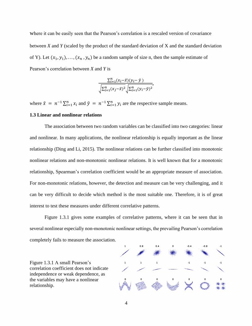
Figure 1.3.1 gives some examples of correlative patterns, where it can be seen that in

several nonlinear especially non-monotonic nonlinear settings, the prevailing Pearson’s correlation

completely fails to measure the association.

Figure 1.3.1 A small Pearson’s

correlation coefficient does not indicate

independence or weak dependence, as

the variables may have a nonlinear

relationship.

5

In this thesis, we aim to compare the statistical performance (in terms of both correlation

strength and significance) of six different measures, including Spearman’s correlation, mutual

information, maximal information coefficient, biweight midcorrelation, distance correlation, and

copula correlation, under many different simulation settings, such as linear, cube root, quadratic,

wavelet, circle, and cluster (Figure 1.3.2).

(a) Low level of noise (b) High level of noise

Figure 1.3.2 Correlative patterns such as linear, cube root, quadratic, wavelet, circle, and

cluster with different levels of noise.

6

Table 1.3.1 below lists all the six correlative patterns with equations that we used for simulation

studies. It should be noted that all the noise term follows a normal distribution with mean 0 and

variance that will be varied in different settings.

Table 1.3.1

Simulation settings considered in this work

Setting Equation Domain

Linear y = 2𝑥 + 𝜀 0 < 𝑥 < 1

Cube Root y = 20𝑥1/3 + 𝜀 0 < 𝑥 < 1

Quadratic y = 2𝑥2 + 𝜀 −1 < 𝑥 < 1

Wavelet y = 2𝑠𝑖𝑛 𝑥 + 𝜀 −2𝜋 < 𝑥 < 2𝜋

Circle X = (5 + εx) cos θ, y = (5 + εy) sin θ

where εx and εy are independent

0 < 𝜃 < 2𝜋

Cluster 𝑥1 = −50 + 𝜀𝑥1, 𝑦1 = 50 + 𝜀𝑦1

𝑥2 = 50 + 𝜀𝑥2, 𝑦2 = 50 + 𝜀𝑦2

𝑥3 = −50 + 𝜀𝑥3, 𝑦3 = −50 + 𝜀𝑦3

𝑥4 = 50 + 𝜀𝑥4, 𝑦4 = −50 + 𝜀𝑦4

where 𝜀𝑥1, 𝜀𝑥2

, 𝜀𝑥3 and 𝜀𝑥4

are independent,

𝜀𝑦1, 𝜀y2

, 𝜀y3 and 𝜀y4

are independent

7

Chapter 2

Methodology

In this section, we review the definitions and statistical properties of the six selected measures.

2.1 Spearman’s rank based correlation

Spearman’s correlation coefficient is defined as the correlation of ranks. It is designed to

measure the monotonic relation between two variables. Spearman’s correlation can be used on

both continuous and ordinal categorical data. Similar to Pearson’s correlation, Spearman’s

correlation is always between -1 and 1. It is a negative value if one variable increases as the other

decreases (da Costa, 2015). However, unlike Pearson’s correlation coefficient, Spearman’s

correlation does not rely on the normal assumption (Bolboaca & Jantschi. 2006). Let 𝑋 =

(𝑥1, … , 𝑥𝑛) and 𝑌 = ( у1, … , у𝑛) be a random sample of size n, Spearman’s correlation 𝒓𝒔 is

defined as follows

𝑟𝑠(𝑥, 𝑦) = 1 −6 ∑ 𝑑𝑖

2𝑖

𝑛(𝑛2−1),

where n is the total number of samples of two variables, and for each random variable, the rank

difference of the ith element is di. It can be proved that rs(x,y) = 0 indicates monotonic independence.

2.2 Mutual information

Another critical measure of linear and nonlinear dependence is mutual information (MI),

which is motivated by the amount of information that two-variable are sharing. The concept of

mutual information was used from the theory of communication by Shannon (1948), who

defined the entropy of a single random variable. Let 𝑋 be a random variable having probability

density function 𝑓1(𝑋), then the entropy H(𝑋) = − ∑ 𝑝𝓃𝒾=1 (𝑥𝑖) log 𝑝(𝑥𝑖) = − 𝐸 log 𝑓1(𝑋). It is

well known that entropy is a measure of uncertainty. Also, entropy satisfies the property that H

8

(𝑋) ≥ 0 is nonnegative. The above definition of entropy extends to a pair of random variables (X,

Y) with joint probability density function f (x, y). We define the joint entropy of (X, Y) as H (X,

Y) = − 𝐸 log 𝑓 (𝑋, 𝑌).

Let X and Y be the two random variables with marginal probability density functions as 𝑓1(X)

and 𝑓2(𝑌), respectively. With given Y, the conditional density function of X is 𝑓(𝑥, 𝑦)/𝑓2(𝑦)

and the conditional entropy is

H (X|Y) = − 𝐸 log𝑓(𝑋,𝑌)

𝑓2(𝑌)

Mutual information 𝐼(𝑋, 𝑌) calculates the amount of information gained from one random variable

(Figure 2.2.1).

𝐼(𝑋, 𝑌) = 𝐻(𝑋) − 𝐻(𝑋|𝑌)

= 𝐻(𝑋) + 𝐻(𝑌) − 𝐻(𝑋, 𝑌)

= ∑ 𝑃(𝜒) 𝑙𝑜𝑔 (1

𝑃(𝜒))𝑥 + ∑ 𝑃(𝑦) 𝑙𝑜𝑔 (

1

𝑃(𝑦))𝑦 + ∑ 𝑃𝑥,𝑦 (𝑥, 𝑦)𝑙𝑜𝑔𝑃(𝑥, 𝑦)

= ∑ 𝑃(𝜒, 𝑦) 𝑙𝑜𝑔 (1

𝑃(𝜒))𝑥,𝑦 + ∑ 𝑃(𝑥, 𝑦) 𝑙𝑜𝑔 (

1

𝑃(𝑦))𝑥,𝑦 + ∑ 𝑃𝑥,𝑦 (𝑥, 𝑦)𝑙𝑜𝑔𝑃(𝑥, 𝑦)

= ∑ 𝑃𝑥,𝑦 (𝑥, 𝑦) 𝑙𝑜𝑔(𝑃(𝑥,𝑦)

𝑃(𝑥)𝑃(𝑦))

Mutual information (MI) measures the amount of information in units (bits). For discrete random

variables with joint probability mass function P (x, y), the MI is defined as

Figure 2.2.1 Venn diagram showing the

relationships between MI and entropies

(Wikipedia,2019).

9

𝐼(𝑋, 𝑌 ) = ∑ ∑ 𝑃𝜘∈𝑋𝑦∈𝑌 (𝜒, 𝑦) log(𝑃(𝜒,𝑦)

𝑃(𝜒)𝑃(𝑦)).

For continuous random variables with joint probability density function f (x, y), the MI can be

defined as

I (X,Y) = ∫ ∫ ƒ(𝑋, 𝑌) logƒ(𝑋,𝑌)

𝑓1(𝑋)𝑓2(𝑦)𝑑𝑥𝑑𝑦

∞

−∞

∞

−∞.

An equivalent way of defining 𝐼(𝑋, 𝑌) between the two variables 𝑋 and 𝑌 is

𝐼(𝑋, 𝑌) = 𝐻(𝑋) + 𝐻(𝑌) − 𝐻(𝑋, 𝑌),

where 𝐻(𝑋), 𝐻(𝑌) are the entropies of X and Y, and 𝐻(𝑋, 𝑌) is the joint entropy between 𝑋 and

𝑌. The term entropy measures the uncertainty of a random variable.

The entropy and mutual information are related through the following derivation

𝐼(𝑋, 𝑌)= E𝑙𝑜𝑔 (1

𝑓1(X).

𝑓(𝑋,𝑌)

𝑓2(𝑌))

= E (−𝑙𝑜𝑔𝑓1(𝑋) + 𝑙𝑜𝑔𝑓(𝑋,𝑌)

𝑓2(𝑌))

= −E𝑙𝑜𝑔 𝑓1(𝑋) + E𝑙𝑜𝑔𝑓(𝑋,𝑌)

𝑓2(𝑌)

= 𝐻(𝑋) + 𝐻(𝑌) − 𝐻(𝑋, 𝑌).

Since H (X, Y) is symmetric, it follows that I (X, Y) = I (Y, X). Hence, the difference in

uncertainty about X given knowledge of Y equals the difference in uncertainty about Y given

knowledge of X (Kinney & Atwal, 2014). When X and Y are independent, their mutual

information is zero. In other words,

𝑃(𝑋, 𝑌) = 𝑃(𝑋)𝑃(𝑌) 𝑜𝑟 log(𝑃(𝑋,𝑌)

𝑃(𝑋)𝑃(𝑌)) = log 1 = 0.

In the case that the two variables are identical, or functionally related, then the information of X

reveals everything about Y, and the entropy of the random variable become equivalent to the

mutual information, 𝐼(𝑋, 𝑌 ) = 𝐻(𝑋) = 𝐻(𝑌 )

10

2.3 Maximal information coefficient

Another popular dependence measure is the maximal information coefficient (MIC).

Reshef et al. (2011) introduced the notion of maximal information coefficient which could

potentially measure both linear and non-linear relationships between variables. Tang et al. (2014)

stated the MIC can be useful in the large datasets to measure the associations between the

thousands of variable pairs. As it takes values between 0 and 1, MIC could not reflect the

directional movement. There are two fundamental properties of MIC, including equitability and

generality. Generality indicates that the statistic must capture a wider variety of associations, such

as periodic, exponential, or linear, with an adequately larger sample size. Equitability shows that

MIC provides similar scores for similarly noisy relationships, irrespective of what type of the

relation is.

As the sample size goes to infinity, MIC almost surely gives score of 1 to every functional

relationship and gives score of 0 to statistically independent variables. There is not any parametric

or distributional assumption in the MIC. MIC is defined by Reshef et al. as the maximum taken

over all x-by-y grids G up to a given grid resolution, {𝐼 (χ,y)

log2 𝑚𝑖𝑛{𝑛X,𝑛y}} based on the empirical

probability distribution over the boxes of a grid G. For two random variables X and Y having

sample n ≥ 2, the MIC is defined as follows

MIC = ⅿax {𝐼 (𝑥 ,y)

log2 𝑚𝑖𝑛{𝑛𝑥 ,𝑛y}} ,

where 𝐼(𝑥, y ) = 𝐻(𝑥) + 𝐻(y ) − 𝐻(𝑥, y ), i.e.,

𝐼(χ, y ) = ∑ 𝒫𝑛χ

𝑖=1(χ𝑖) log2

1

𝒫(χ𝑖) + ∑ 𝒫

𝑛y

𝑖=1(y𝑖) log2

1

𝒫(y𝑖) − ∑ ∑ 𝒫

𝑛y

𝑖=1(χ𝑖, y𝑖) log2

1

𝒫(χ𝑖,y𝑖)

𝑛χ

𝑖=1

11

where, 𝑛𝑥 𝑎𝑛𝑑 𝑛y represents the bins between the partition of the axes. 𝑛𝑥 . 𝑛y < 𝐵(𝑛), 𝐵(𝑛) =

𝑛0.6 . Nguyen et al. (2014) pointed out the maximal correlation does not require assumptions on

the distribution of data. It appears robust and very efficient, and it can also detect nonlinear

correlation.

2.4 Biweight midcorrelation

Biweight midcorrelation (bicor) is based on the measure of similarity between variables.

There are two major advantages for bicor. First, the calculation is straightforward, consisting of

some simple steps such as the calculation of median. Second, it is more robust to outliers

comparing to other measures such as Spearman’s correlation (Yuan et al., 2013).

To define the biweight midcorrelation (bicor) of two numeric vectors 𝑥 = (𝑥1, 𝑥2, . . . 𝑥𝑛)

and 𝑦 = (𝑦1, 𝑦2, . . . 𝑦𝑛), we must define 𝑎𝑖 , 𝑏𝑖 with 𝑖 = 1,2, . . . , 𝑛, where 𝑚𝑒𝑑(𝑥) is the median

and 𝑚𝑎𝑑(𝑥) is the absolute median deviation of 𝑥:

𝑎𝑖 =𝑥𝑖 − 𝑚𝑒𝑑(𝑥)

9𝑚𝑎𝑑(𝑥)

Similarly, we define 𝑏𝑖, where 𝑚𝑒𝑑(𝑦) is the median and 𝑚𝑎𝑑(𝑦) is the absolute median deviation

of 𝑦:

𝑏𝑖 =𝑦𝑖 − 𝑚𝑒𝑑(𝑦)

9𝑚𝑎𝑑(𝑦)

where 𝑚𝑒𝑑(𝑥) is the median and 𝑚𝑎𝑑(𝑥) is the absolute median deviation,

𝑚𝑎𝑑(𝑥) = 𝑚𝑒𝑑(|𝑥𝑖 − 𝑚𝑒𝑑(𝑥)|)

These equations are used to define weight, 𝑚𝑖. For X, the weight is defined as

𝑚𝑖(𝑥)

= (1 − 𝑎𝑖2)2𝐼(1 − |𝑎𝑖|),

12

where I is the identity function. Yuan et al. (2013) mentioned that the indicator is 1 when 𝐼(1 −

|𝑎𝑖|) > 0 and is 0 when 𝐼(1 − |𝑎𝑖|) ≤ 0. Using the definition of weight to normalize so that the

sum of the weights is 1

𝑥�̃� =(𝑥𝑖 − 𝑚𝑒𝑑(𝑥))𝑚𝑖

(𝑥)

√∑ [(𝑥𝑗𝑛𝑗=1 − 𝑚𝑒𝑑(𝑥))𝑚𝑗

(𝑥)]2

, 𝑦�̃� =(𝑦𝑖 − 𝑚𝑒𝑑(𝑦))𝑚𝑖

(𝑦)

√∑ [(𝑦𝑗𝑛𝑗=1 − 𝑚𝑒𝑑(𝑦))𝑚𝑗

(𝑦)]2

𝑏𝑖𝑐𝑜𝑟(𝑥, 𝑦) =∑ (𝑥𝑖

𝑛𝑖=1 − 𝑚𝑒𝑑(𝑥))𝑚𝑖

(𝑥)(𝑦𝑖 − 𝑚𝑒𝑑(𝑦))𝑚𝑖

(𝑦)

√∑ [(𝑥𝑗𝑛𝑖=1 − 𝑚𝑒𝑑(𝑥))𝑚𝑗

(𝑥)]2√∑ [(𝑦𝑘

𝑛𝑘=1 − 𝑚𝑒𝑑(𝑦))𝑚𝑘

(𝑦)]2

Biweight midcorrelation has many successful applications, for instance, gene co-

expression analysis and gene community (clique) detection(Zeng et al., 2013). To study gene co-

expression, DNA microarray data have been widely used. Genes and their protein products tend

to work in cooperation rather than in isolation. However, most of the existing studies focused on

single gene or single type of genetic data and overlooked the interactions between genes and other

factors. Maxim clique concept was used to further look into the Signaling pathways involving

multiple genes or biomarkers. The most commonly used correlation is Pearson correlation. Other

proposed approaches include biweight midcorrelation and half-thresholding strategy. Being more

robust to outliers, the biweight midcorrelation has a whip hand over Pearson correlation plus

experiments on simulated datasets have proven it to have better performance (Zeng et al., 2013).

2.5 Distance correlation

Distance correlation is a novel measure of dependence between two sets of random

variables of arbitrary dimension. The distance correlation between two random vectors X and Y

(Székely, Rizzo & Bakirov, 2007) is described as a rescaled distance covariance (same as

Pearson’s correlation in spirit)

𝑑𝐶𝑜𝑟(𝑋, 𝑌) = 𝑑𝐶𝑜𝑣(𝑋, 𝑌)/√𝑑𝐶𝑜𝑟(𝑋, 𝑋)𝑑𝐶𝑜𝑟(𝑌, 𝑌)

13

where the squared distance covariance is defined as 𝑑𝐶𝑜𝑣2(𝑋, 𝑌) = 𝐶𝑜𝑣(∥ 𝑥1 − 𝑥2 ∥, ∥ 𝑦1 −

𝑦2 ∥) − 2 𝐶𝑜𝑣(∥ 𝑥1 − 𝑥2 ∥, ∥ 𝑦1 − 𝑦2 ∥), and a natural estimator of 𝑑𝐶𝑜𝑣2(𝑋, 𝑌) 𝑖𝑠

𝑑𝐶𝑜�̂�2(𝑋, 𝑌) = ∑ ∑𝐴𝑖𝑗𝐵𝑖𝑗

𝑛2𝑛𝑗=1

𝑛𝑖=1 ,

where 𝐴𝑖𝑗 = 𝑎𝑖𝑗 − 𝑎�̅� − 𝑎�̅� + �̅� and 𝐵𝑖𝑗 = 𝑏𝑖𝑗 − 𝑏�̅� − 𝑏�̅� + �̅�, if we let 𝑎𝑖𝑗 = ‖𝑋𝑖 − 𝑋𝑗‖,

𝑎�̅� = ∑ ∑‖𝑋𝑅−𝑋𝑖‖

𝑛

𝑛𝑙=1

𝑛𝑘=1 , 𝑎�̅� = ∑

‖𝑋𝑙−𝑋𝑗‖

𝑛

𝑛𝑙=1 , �̅� = ∑

‖𝑋𝑙−𝑋𝑘‖

𝑛2𝑛𝑘=1 , let 𝑏𝑖𝑗 = ‖𝑌𝑖 − 𝑌𝑗‖,

𝑏�̅� = ∑‖𝑌𝑅−𝑌𝑖‖

𝑛

𝑛𝑘=1 , 𝑏�̅� = ∑

‖𝑌𝑙−𝑌𝑗‖

𝑛

𝑛𝑙=1 , �̅� = ∑ ∑

‖𝑌𝑙−𝑌𝑘‖

𝑛2𝑛𝑙=1

𝑛𝑘=1 . The estimate of distance

correlation 𝑑𝐶𝑜�̂�(𝑋, 𝑌) = 𝑑𝐶𝑜�̂�(𝑋,𝑌)

√𝑑𝐶𝑜�̂�(𝑋,𝑋)𝑑𝐶𝑜�̂�(𝑌,𝑌).

Two remarkable properties of distance correlation are

1. 0 ≤ 𝑑𝐶𝑜𝑟 (𝑋, 𝑌) ≤ 1: In comparison to negative Pearson’s correlation, this is always

positive.

2. 𝑑𝐶𝑜𝑟 (𝑋, 𝑌) = 0 if and only if X and Y are independent.

2.6 Copula correlation

Copula correlation is a dependence measure of the deterministic relationship using hidden

uniform noise. The copula function for any random vector Χ1, Χ2, … . . Χ𝑛 is defined as

𝐹(𝑥1, 𝑥2, … . . 𝑥𝑛) = 𝐶(𝐹1(𝑥1), 𝐹2(𝑥2), … 𝐹𝑛(𝑥𝑛)),

where 𝐹 stands for the joint cumulative distribution function and 𝐹1(𝑥1), 𝐹2(𝑥2), … 𝐹𝑛(𝑥𝑛) are the

marginal cumulative distribution function. By Sklar’s theorem (Sklar (1959)), one can decompose

the joint distribution function into the copula form of its marginals. Moreover, the joint density is

𝑓(𝑥1, 𝑥2, … . . 𝑥𝑛) = 𝑓1(𝑥1) ∗ … ∗ 𝑓𝑛(𝑥𝑛)𝐶(𝐹1(𝑥1), 𝐹2(𝑥2), … , 𝐹𝑛(𝑥𝑛)).

Given that 𝐹𝑖 and 𝐶 are differentiable, 𝐶 = 𝜕𝑛 𝐶

(𝜕𝐹1 . . . 𝜕𝐹𝑛). Under the limited scenario, the joint

probability density function is the product of the copula density and the marginal densities. For

14

example, if the i random variables 𝑋𝑖’s are independent, then 𝐶 = 1 and 𝑓(𝑥1, 𝑥2, … . . 𝑥𝑛) =

𝑓1(𝑥1) ∗ … ∗ 𝑓𝑛(𝑥𝑛). Clemen and Reilly (1999) state that the n-dimensional joint distribution

function F has two components (1) copula function, and (2) marginal distribution function. Let

𝑋 = (𝑋1, 𝑋2,· · ·, 𝑋𝑛) be a random vector with distribution function F, and Y be uniformly

distributed on (0, 1) and independent of X. We know that Ui = Fi (Xi, Y) is uniformly distributed

on (0, 1), therefore Xi = Fi −1 (Ui). If we let the copula C be the distribution function of U = (U1,

U2, · · ·, Un), then we have

F(X) = P (X ≤ x)

= P (Fi −1 (Ui) ≤ xi, 1 ≤ i ≤ n)

= P (Ui ≤ Fi(xi), 1 ≤ i ≤ n)

= C(F1(x1), · · ·, Fn(xn)).

This implies that C is the copula of F. Conveniently, a joint distribution function F(x,y) can be

written in terms of the marginal distribution functions FX(x) and FY(y) for the random variable X

and Y using the relation F(x,y) = C(FX(x), FY(y)). Hence, the copula function C(u, v) can be written

as

𝐶(𝑢, 𝑣) = 𝐹(𝐹𝑋−1(𝑢), 𝐹𝑌−1(𝑣)),

and immediately it follows that

𝐶(𝐹𝑥(𝑥), 𝐹𝑦(𝑦)) = 𝐹(𝐹𝑋−1(𝐹𝑥(𝑥)), 𝐹𝑌−1(𝐹𝑦(𝑦))) = 𝐹(𝑥, 𝑦).

For calculating copula distance between the copula density c (x,y) and the independence copula

density by using 𝐿𝑝 distance, 𝐶𝐷𝛼 =∬|𝑐(𝑥, 𝑦) − 1|𝛼𝑑𝑥𝑑𝑦, α > 0. 𝐶𝐷2 is the Pearson’s ∅2 with

its scaled version being ∅cor = √𝐶𝐷/(1 + 𝐶𝐷2). Particularly, the copula correlation is a scale

version of 𝐶𝐷1 as Ccor = 1

2𝐶𝐷1 =

1

2∬ | 𝑐(𝑥, 𝑦) − 1|𝑑𝑥𝑑𝑦.

15

Chapter 3

Simulation studies and real data application

In this section, we compare all the six dependence measures in terms of the statistical power

using under various simulation settings, including Spearman’s correlation, mutual information,

maximal information coefficient, biweight midcorrelation, distance correlation, and copula

correlation. A real genomic application is also provided. For a complete picture about how these

measures work in different correlative patterns, we considered linear, cube root, quadratic,

wavelet, circle, and cluster settings.

3.1 Simulated studies

We conducted simulation studies with the inclusion of the noise. The purpose of including

the additive noise is to increase randomness and to test the robustness of the correlation measures.

We considered both relatively low and high levels of additive noise. The R-packages for our

implementation include pspearman, minerva, wgcna, energy, copula, and infotheo. For all settings,

the sample size is fixed at 80.

3.1.1 Spearman’s correlation

We used Fisher’s method to transform Spearman’s correlation coefficient to a z value

𝑧 =1

2 𝑙𝑛 (

1 + 𝑝

1 − 𝑝 ),

where 𝑝 is the Spearman’s rank correlation coefficient. It can be proved that z asymptotically

follows a normal distribution with mean 0.

The two R packages used for this analysis are infotheo and pspearman. Averages of the

resulting p-values were summarized. Figure 3.1.1 and Figure 3.1.2 illustrate the result for all six

patterns with different levels of noise. The results were based on 80 samples.

16

Figure 3.1.1 Spearman's rank correlation for linear, cube root, quadratic, wavelet, circle, and

cluster settings with smaller noise.

Figure 3.1.2 Spearman's rank correlation for linear, cube root, quadratic, wavelet, circle, and

cluster settings with larger noise. `

17

Table 3.1.1 showed the empirical statistical power and the average p-value.

Table 3.1.1

Spearman correlation method

Relationship Smaller Noise Larger Noise

Empirical

power

Mean

p-value

Empirical

power

Mean

p-value

Linear 0.825 0.049 0.213 0.333

Cube Root 0.787 0.093 0.254 0.288

Quadratic 0.013 0.607 0.038 0.537

Wavelet 0.788 0.097 0.388 0.141

Circle 0.0 0.686 0.0 0.610

Cluster 0.0 0.973 0.0 0.974

3.1.2 Mutual information

Mutual information (MI) is a measure of information quantity shared between two random

variables. Figure 3.1.3 and Figure 3.1.4 show the result for linear, cube root, quadratic, wavelet,

circle, and cluster setting with mutual information under different levels of noise. Similar to the

Spearman’s correlation, the MI can be converted to z value by Fisher’s z transformation for

independence test. The continuous data are discretized to compute entropy.

Figure 3.1.3 shows the distribution of the p-values with smaller noise. It is apparent that the

variability of an estimate is significantly lower.

18

Figure 3.1.3 Mutual information for linear, cube root, quadratic, wavelet, circle, and cluster

settings with smaller noise.

Figure 3.1.4 Mutual information for linear, cube root, quadratic, wavelet, circle, and cluster

settings with larger noise.

Figure 3.1.4 shows the simulation results for the same model structure but with larger noise

level. Table 3.1.2 shows the statistical result of empirical power and the average p-value with

different number bins (nbins), where it can be seen that the mutual information works well for

cube root, wavelet and circle settings with nbins=1/3 (see table 3.1.2 (a)). However, the mutual

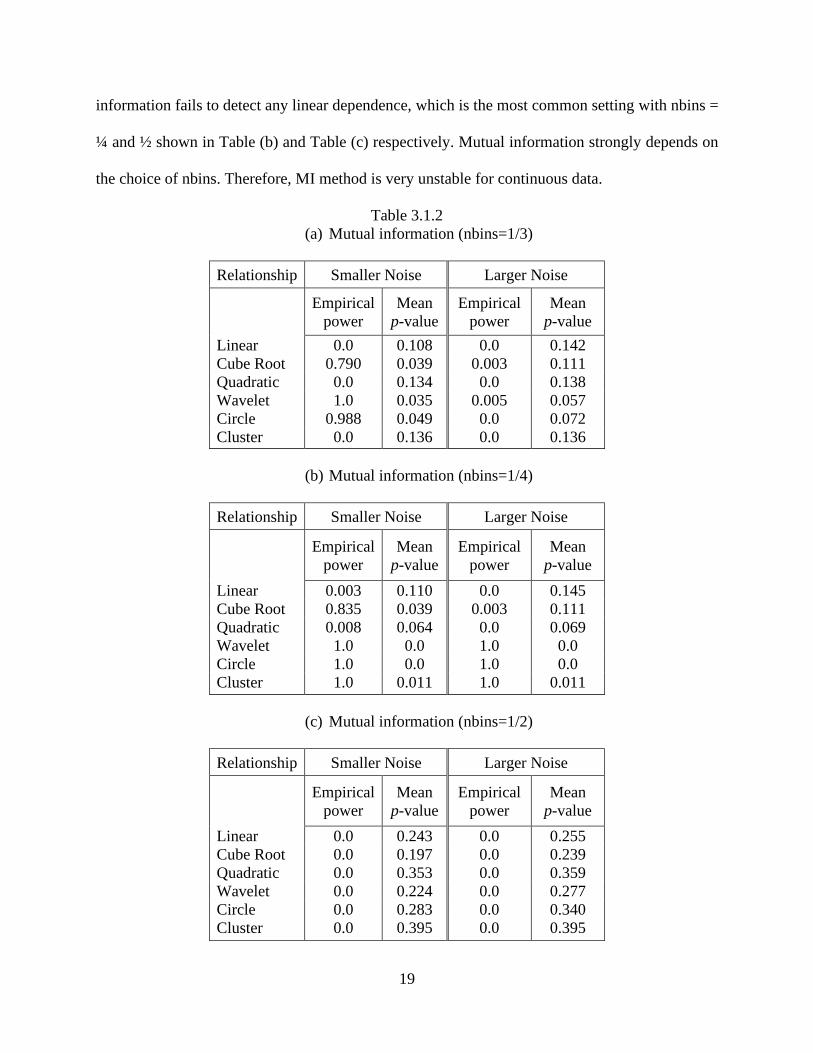
19

information fails to detect any linear dependence, which is the most common setting with nbins =

¼ and ½ shown in Table (b) and Table (c) respectively. Mutual information strongly depends on

the choice of nbins. Therefore, MI method is very unstable for continuous data.

Table 3.1.2

(a) Mutual information (nbins=1/3)

Relationship Smaller Noise Larger Noise

Empirical

power

Mean

p-value

Empirical

power

Mean

p-value

Linear 0.0 0.108 0.0 0.142

Cube Root 0.790 0.039 0.003 0.111

Quadratic 0.0 0.134 0.0 0.138

Wavelet 1.0 0.035 0.005 0.057

Circle 0.988 0.049 0.0 0.072

Cluster 0.0 0.136 0.0 0.136

(b) Mutual information (nbins=1/4)

Relationship Smaller Noise Larger Noise

Empirical

power

Mean

p-value

Empirical

power

Mean

p-value

Linear 0.003 0.110 0.0 0.145

Cube Root 0.835 0.039 0.003 0.111

Quadratic 0.008 0.064 0.0 0.069

Wavelet 1.0 0.0 1.0 0.0

Circle 1.0 0.0 1.0 0.0

Cluster 1.0 0.011 1.0 0.011

(c) Mutual information (nbins=1/2)

Relationship Smaller Noise Larger Noise

Empirical

power

Mean

p-value

Empirical

power

Mean

p-value

Linear 0.0 0.243 0.0 0.255

Cube Root 0.0 0.197 0.0 0.239

Quadratic 0.0 0.353 0.0 0.359

Wavelet 0.0 0.224 0.0 0.277

Circle 0.0 0.283 0.0 0.340

Cluster 0.0 0.395 0.0 0.395

20

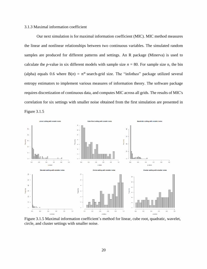
3.1.3 Maximal information coefficient

Our next simulation is for maximal information coefficient (MIC). MIC method measures

the linear and nonlinear relationships between two continuous variables. The simulated random

samples are produced for different patterns and settings. An R package (Minerva) is used to

calculate the p-value in six different models with sample size n = 80. For sample size n, the bin

(alpha) equals 0.6 where B(n) = 𝑛α search-grid size. The “infotheo” package utilized several

entropy estimators to implement various measures of information theory. The software package

requires discretization of continuous data, and computes MIC across all grids. The results of MIC's

correlation for six settings with smaller noise obtained from the first simulation are presented in

Figure 3.1.5

Figure 3.1.5 Maximal information coefficient’s method for linear, cube root, quadratic, wavelet,

circle, and cluster settings with smaller noise.

21

The average p-value ranges from 0.012 to 0.690. Observably, most settings did not show a

good strength of the dependence linear or nonlinear relationship within a noise-free environment.

Figure 3.1.6 shows MIC's correlation for six settings with a larger noise. The mean of all p- values

are high, and hence, MIC performs poorly to detect measure dependence for linear and nonlinear

relationships.

Figure 3.1.6 Maximal information coefficient’s method for linear, cube root, quadratic, wavelet,

circle, and cluster settings with larger noise.

Table 3.1.3 shows the empirical statistical power and the average p-value.

Table 3.1.3

Maximal information coefficient

Relationship Smaller Noise Larger Noise

Empirical

power

Mean

p-value

Empirical

power

Mean

p-value

Linear 0.548 0.065 0.225 0.209

Cube Root 0.225 0.279 0.087 0.406

Quadratic 0.713 0.065 0.20 0.254

Wavelet 0.875 0.012 0.188 0.322

Circle 0.0 0.690 0.013 0.707

Cluster 0.038 0.479 0.025 0.596

22

3.1.4 Biweight midcorrelation

Biweight midcorrelation (bicor) is median based, which reduces sensitivity to outliers.

Consequently, the results of simulations prove that the bicor performs better in identifying the

uncertainty in the dependent variable when the independent variable is observed. The graphs

presented using the bicor method demonstrates a measure of the similarity levels. However, the

statistical method depends on the R-language, which interprets multiple data and variables. The

package components used for bicor are (BiocManager) and the library (WGCNA).

The R package WGCNA includes functions corAndPvalue and bicorAndPvalue that

calculate correlations of matrices and their associated Student p -values efficiently and accurately

(Langfelder and Horvath 2008).

Figure 3.1.7 Biweight midcorrelation’s method for linear, cube root, quadratic, wavelet, circle,

and cluster settings with smaller noise.

23

The two main parameters considered to generate the average method in the formula are

median pseudo ranks and weight pseudo ranks. Some distributions in Figure 3.1.7 indicate the

obtainability of strong association for linear and nonlinear relationship among smaller noise

models. For example, linear, cube root, and wavelet have mean p- values less than statistical

significance level, while quadratic, circle, and cluster do not detect measure of dependence since

the mean p-value is greater than 5%. Whereas the distributions of large noise models do not

perform good quality in this case as shown in Figure 3.1.8. Circle and cluster represent the

highest p-value than the other models.

Figure 3.1.8 Biweight midcorrelation’s method for linear, cube root, quadratic, wavelet, circle,

and cluster settings with larger noise.

The summary of p-values is presented in Table 3.1.4, where it can be seen that biweight

midcorrelation is able to provide quality results for linear cube root and wavelet.

24

Table 3.1.4

Biweight midcorrelation

Relationship Smaller Noise Larger Noise

Empirical

power

Mean

p-value

Empirical

power

Mean

p-value

Linear 0.813 0.029 0.200 0.207

Cube Root 0.715 0.045 0.150 0.306

Quadratic 0.006 0.543 0.059 0.514

Wavelet 0.744 0.039 0.188 0.157

Circle 0.0 0.607 0.0 0.832

Cluster 0.0 0.758 0.0 0.917

3.1.5 Distance correlation

The following simulation considered is the distance correlation (dcor) measure. It is

equivalent to product-moment covariance and correlation. The test for dependence relationships is

considered for different settings with distance correlation and the two different levels of noise. The

samples were randomly generated from the normal distribution with sample size, n = 80. The result

was tested for the significance level of 5%. The dcor R-package helps in analyzing the multivariate

data. The correlation process applies to both the larger noise and the smaller noise data sets,

depending on the distance. For the dcor package library (energy) was used to derive the codes in

the R-Program with a distance correlation test. 5000 permutations were considered to get a more

accurate result.

25

Figure 3.1.9 Distance’s correlation for linear, cube root, quadratic, wavelet, circle, and cluster

settings with smaller noise.

Figure 3.1.9 summarizes the simulation results for linear, cube root, quadratic, wavelet,

circle, and cluster setting with distance correlation smaller noise. It appears that the wavelet model

would get perfect strength of that dependence within the variety of noise, likewise the linear

function. Figure 3.1.10 illustrates the results of six functions for larger noise. The result

demonstrates that none of the settings identify the dependence test.

26

Figure 3.1.10 Distance’s correlation for linear, cube root, quadratic, wavelet, circle, and cluster

settings with larger noise.

Table 3.1.5. illustrates the empirical statistical power and the average p-value, where it can

be seen that the distance measure is sensitive to linear cube root, quadratic and wavelet

dependence.

Table 3.1.5

Distance correlation

Relationship Smaller Noise Larger Noise

Empirical

power

Mean

p-value

Empirical

power

Mean

p-value

Linear 0.863 0.019 0.213 0.344

Cube Root 0.740 0.099 0.150 0.443

Quadratic 0.751 0.037 0.101 0.326

Wavelet 0.963 0.011 0.550 0.073

Circle 0.541 0.073 0.0 0.442

Cluster 0.0 0.414 0.0 0.449

27

3.1.6 Copula correlation

The copula cluster is an R-package for the implementation of the clustered algorithm.

The copula function found data sets for the complex multivariate dependence to produce the

process. The normal distributed data with sample size n = 80 and a significance level of 5% was

considered for simulation. The number of permutations considered during the simulation is 1000.

Figure 3.1.11 Copula correlation for linear, cube root, quadratic, wavelet, circle, and cluster

settings with smaller noise.

Figure 3.1.11 illustrates the results for linear, polynomial, quadratic, wavelet, circle, and

cluster setting with Ccor smaller noise generated from a normal distribution. Monotonic

relationships are common when interpretation depends on the copula correlation method. The

quadratic, cluster, and circle setting graphs indicate a variety of parameters that affect the data

analysis to attain the spectrum range. Copula correlation gives a high p-value of the setting since

28

they are nonlinear relationships. The copula correlation displays the function of both smaller and

significant noise data types. Ccor analysis depends on the linear bivariate relationship.

Figure 3.1.12 summarizes the p-values for larger noise.

Figure 3.1.12 Copula correlation for linear, cube root, quadratic, wavelet, circle, and cluster

settings with larger noise.

Table 3.1.6 shows the empirical statistical power and the average p-value, where it can be

seen that the copula correlation has satisfactory performance only for linear setting.

29

Table 3.1.6

copula correlation

Relationship Smaller Noise Larger Noise

Empirical

power

Mean

p-value

Empirical

power

Mean

p-value

Linear 0.789 0.029 0.213 0.306

Cube Root 0.462 0.082 0.150 0.334

Quadratic 0.338 0.128 0.075 0.500

Wavelet 0.138 0.269 0.050 0.532

Circle 0.175 0.257 0.0 0.625

Cluster 0.101 0.497 0.060 0.505

Table 3.1.7 summarizes the overall performance of each measure.

Table 3.1.7

Simulation performance of different settings

Measures Simulation settings with overall satisfactory

performance

Spearman’s rank correlation Linear, Cube Root, Wavelet

Mutual information Cube Root, Wavelet, Circle

Maximal information coefficient Quadratic, Wavelet

Biweight midcorrelation Linear, Cube Root, Wavelet

Distance correlation Linear, Cube Root, Quadratic, Wavelet, Circle

Copula correlation Linear

The above results show that Spearman’s correlation, biweight midcorrelation and distance

correlation have overall satisfactory performance for linear and nonlinear relationships.

30

3.2 A genomic application

In this part, we applied some selected measures to a dataset from the Cancer Genome

Atlas (TCGA), pre-processed by Zhang et al. (2014). The dataset contained the expression level

of 245 cancer-related genes from 150 samples. The analysis focuses on the detection of co-

expressed genes using three measures that have overall good performance from simulation

studies, including Spearman’s rank, distance correlation and biweight midcorrelation.

Gene co-expression analysis has been widely applied for molecular biology research,

especially for the systems-level or pathway-level studies. In general, the functions in isolation of

genes and their protein products do not perform. The functions perform jointly and in

cooperation. Tremendous research efforts have been made to clarify the molecular basis of the

initiation and progression of ovarian cancer. However, most of those studies have concentrated

on a single gene or a specific type of data, which in return may not identify the complex

mechanisms of cancer formation by neglecting to detect the interactions of different genetic and

epigenetic factors (Zhang et al., 2014). In practice, temporal changes in gene expression require

more complex detection methods than simple correlation measures that may result in complex

association patterns. For example, the effect of regulation may lead to time-lagged associations

and interactions local to a subset of samples.

31

Figure 3.2.1 Histogram of TCGA ovarian cancer data using Spearman’s method including the

correlation measure (left panel), and p-value (right panel), from 5000 replications

Figure 3.2.1 summarized the Spearman’s rank correlation for more than 20,000 pairs of genes

that are significantly associated (p < 0.05).

For dcor, the energy package was used with index =1, which is the exponent on

Euclidean distance. Euclidean distance ∥xi−xj∥d, where 0 < d < 2 to compute distance

correlation and p-value. Figure 3.2.2 shows the distribution of correlation and p-value by using

dcor method. We found more than 25,000 pairs of genes having p-value less than 5%.

32

Figure 3.2.2 Histogram of TCGA ovarian cancer data using distance method including the

correlation measure (left side), and p-value (right side), with 5000 number of replications

Finally, the co-expression of all gene pairs were measured by biweight midcorrelation

measure. It concentrates on the media-based analysis, which diminished sensitivity towards the

outliers. To compute the biweight midcorrelation (bicor) between pairs of genes, the WGCNA

package was used to compute correlation measure and p-value. In the histogram which are

demonstrated in Figure 3.2.3, it is noticeable that there is a significant correlation for more than

20,000 pairs after replication while the correlation measure shows a strong correlation

considering that the majority of the gene pairs are dependent.

33

Figure 3.2.3 Histogram of TCGA ovarian cancer data using biweight midcorrelation including

the correlation measure (left panel), and p-value (right panel).

We then investigated the consistency between the three measures. The figure 3.2.4 below

show the agreement between each pair of measures: (A) Spearman’s correlation vs biweight

midcorrelation; (B) Spearman’s correlation vs distance correlation; (C) Biweight midcorrelation

vs distance correlation.

34

(A) (B)

(C)

Figure 3.2.4 Comparison of correlations: (A) Spearman’s correlation coefficient vs. biweight

midcorrelation, (B) Spearman’s correlation coefficient vs. distance correlation, and (C)

distance correlation vs. biweight midcorrelation.

35

As can be seen from Figure 3.2.4, for the majority of co-expressed gene pairs, especially those

with strong co-expression, all three measures are similar. Table 3.2.1 presents in 6 pairs of

strongly correlated genes as examples. Our findings confirm some recent reports that the

majority of co-expressed genes are linear or monotonic nonlinear.

Table 3.2.1

Examples of co-expressed gene pairs by Spearman’s rank correlation, biweight midcorrelation

and distance correlation

Gene pairs

( i, j )

Spearman

correlation

Biweight

midcorrelation

Distance

correlation

(42,188) 0.8083 0.8224 0.7891

(47,199) 0.7917 0.8119 0.7766

(88,244) 0.8190 0.8356 0.8282

(89,244) 0.7735 0.7987 0.7932

(190,235) 0.8397 0.8585 0.8233

(196,214) 0.8031 0.8002 0.7753

36

Chapter 4

Conclusions

In many scientific domains, it is essential to identify and measure different types of

associative relations between variables from experimental or observational data. The relationship

between two variables is often characterized by some type of correlation coefficient, which can

be utilized for further decision-making and predictions. Pearson’s correlation coefficient is

popular as a measure of strength of the relationship between two variables. The procedure,

however, is limited to linear associations and is excessively sensitive to outliers. To measure

nonlinear-type relations, a number of correlation measures have been recently developed,

including distance correlation, MIC, mutual information, etc. In this work, we conduct an

extensive simulation study to systematically compare these measures in various settings. Based

on our simulation result, Spearman’s correlation, biweight midcorrelation and distance

correlation have better statistical performance overall. They can be robust alternatives to other

statistical measures, especially when the underlying relation is nonlinear. The mutual

information does not work well in linear settings, and the performance depends on discretization

for continuous data.

4.1 Discussion

We would like to point out that all the dependence measures considered in this thesis have

certain drawbacks. For instance, it is known that MIC depends on a user-defined parameter,

namely B(n). Also, the computational cost of MIC increases exponentially as the number of data

points gets larger; therefore, it is not suitable for large-scale datasets. Additionally, as pointed out

by Simon and Tibshirani (2014), MIC may not work well in the presence of substantial noise.

37

Kinney and Atwal (2014) also noted that MIC is not equitable, and the MIC values might not be

affected by variable noise for specific relationships.

Although mutual information is a popular measure of nonlinear or combinatorial

dependence between two variables, it has been pointed out that the estimate of MI measure could

be challenging for small datasets due to the discretization and number of bins. In addition, MI does

not satisfy the criterion of equitability (equitability is a criterion that the statistic should give

similar scores to equally noisy relationships of different types). Thus, it is not a reliable method

for continuous data.

MIC and distance correlation are two promising measures for nonlinear relations. Simon

and Tibshirani (2014) state that in many cases, distance correlation exhibits more statistical power

than the MIC. It can also be seen in our analysis that even with a small sample size, the distance

correlation has satisfactory performance at a different level of noise. Copula correlation could

potentially capture the complete dependence structure inherent in variables (Xi et al., 2014).

However, the copula-based methods are analytically complex and difficult to interpret, and fitting

the parameters of a copula is a challenging statistical problem.

The distance correlation and biweight midcorrelation have overall satisfactory

performance for most of the correlative patterns, with affordable computational cost and good

robustness to outliers. However, there is still a need to find or develop a measure that is

interpretable and sensitive to both linear and nonlinear, monotonic and non-monotonic relations.

4.2 Future work

There are several directions that we would like to explore in the future. First, we will

incorporate some additional measures recently developed to measure nonlinear relations, to name

38

a few, the projection correlation (Zhu et al., 2017), and multiscale graph correlation (MGC, Shen,

Priebe & Vogelstein, 2019).

Second, we may extend the evaluation of correlation measures from univariate variables to

multivariate variables or random vectors of arbitrary dimensions. Compared to model-based

exploration such as multiple linear regression and principal component analysis, the correlation

method is model-free and does not rely on any assumption on the model structures. Also,

categorical variables are commonly seen in many scientific studies. Further analysis can be

conducted by comparing the correlation measures for the association between categorical variables

or even the association between a categorical variable (either ordinal or nominal) and a continuous

variable.

Third, we may test all correlation measures on other, real datasets. For instance, it will be

interesting to apply distance correlation to some genomic datasets to identify nonlinearly

correlated biomarkers or biological pathways. Such analyses may shed new light to the complex

relations between many different types of biological factors.

39

References

Bolboaca, S.-D., and Jantschi, L., 2006. Pearson ¨ versus Spearman, Kendall's tau correlation

analysis on structure-activity relationships of biologic active compounds. Leonardo

Journal of Sciences 5(9):179–200.

Chang, Y., Li, Y., Ding, A., & Dy, J. G. (2016). A robust-equitable copula dependence measure

for feature selection. Proceedings of the 19th International Conference on Artificial

Intelligence and Statistics, AISTATS 2016.

Clemen, R., and Reilly, T. (1999). "correlations and copulas for Decision and Risk Analysis,"

Management Science, Vol. 45(2)

Da Costa, J. P., 2015. Rankings and Preferences: New Results in Weighted Correlation and

Weighted Principal Component Analysis with Applications. Springer.

Deebani, W., & Kachouie, N. N. (2018). Ensemble correlation coefficient. International

Symposium on Artificial Intelligence and Mathematics, ISAIM 2018.

https://doi.org/10.1007/978-3-319-55895-0_17

Ding, A., and Li, Y. (2015). copula correlation: An Equitable Dependence Measure and

Extension of Pearson's correlation. arXiv:1312.7214

Fisher, L. D., & van Belle, G. (1993). Biostatistics: A Methodology for the Health Sciences.

John Wiley and Sons Ltd, New York, United States 1993.

Hastie, T.; Tibshirani, R.; and Friedman, J. 2002. The elements of statistical learning: Data

mining, inference, and prediction. Biometrics.

Kinney, J. B., & Atwal, G. S. (2014). Equitability, mutual information, and the maximal

information coefficient. Proceedings of the National Academy of Sciences of the United

States of America. https://doi.org/10.1073/pnas.1309933111

Langfelder, P., & Horvath, S. (2008). WGCNA: An R package for weighted correlation network

analysis. BMC Bioinformatics. https://doi.org/10.1186/1471-2105-9-559

Li, D. X. (2000). On default correlation: A copula function approach. The Journal of Fixed

Income, 9(4), 43-54.

Martinez-Gomez, E., Richards, M., T. & Richards, D., T. (2014). distance correlation methods

for discovering associations in large astrophysical databases. The Astrophysical Journal,

781 (1)

40

Nguyen, H. V.; Muller, E.; Vreeken, J.; Efros, P.; and B ¨ ohm, ¨ K. 2014. Multivariate maximal

correlation analysis. In Proceedings of the 31st International Conference on Machine

Learning (ICML-14), 775–783.

Reshef, D. N.; Reshef, Y. A.; Finucane, H. K.; Grossman, S. R.; McVean, G.; Turnbaugh, P. J.;

Lander, E. S.; Mitzenmacher, M.; and Sabeti, P. C. 2011. Detecting novel associations in

large data sets. Science 334(6062):1518–1524.

Rüschendorf, L. (2009). On the distributional transform, Sklar's theorem, and the empirical

copula process.

Shannon, C. E. (1948). A mathematical theory of communication. The Bell System Technical

Journal, 27(1):379–423,623–656.

Shen, C., Priebe, C., & Vogelstein, J., (2019) From Distance Correlation to Multiscale Graph

Correlation, Journal of the American Statistical Association, 115:529, 280-

291, DOI: 10.1080/01621459.2018.1543125

Simon, N., & Tibshirani, R. (2014). Comment on “Detecting Novel Associations In Large Data

Sets” by Reshef Et Al, Science Dec 16, 2011. Science. http://arxiv.org/abs/1401.7645

Sklar, A. 1959. Fonctions de Re´partition a` n Dimensions et Leurs

Marges. Publications de l’Institut Statistique de l’Universite´ de. Paris, 8 229–231.

Spearman, C. (2010). The proof and measurement of association between two

things. International journal of epidemiology, 39(5), 1137-1150.

Székely, G. J., Rizzo, M. L., & Bakirov, N. K. (2007). Measuring and testing dependence by

correlation of distances. The annals of statistics, 35(6), 2769-2794.

Tang, D., Wang, M., Zheng, W.,& Wang, H.(2014). RapidMic: Rapid Computation of the

maximal Information Coefficient. Evol Bioinform Online. 10: 11–16. DOI:

10.4137/EBO.S13121

Wang, Y X., Liu, K., Elizabeth, T., Rotter, J., Medina, M., Waterman, M., Huang, H., (2018).

Generalized correlation measure using count statistics for gene expression data with

ordered samples. Bioinformatics, 34(4), 617–624.

https://doi.org/10.1093/bioinformatics/btx641

Wang, Y., Li, Y., Cao, H. et al. (2015). Efficient test for nonlinear dependence of two continuous

variables. BMC Bioinformatics 16: 260.

Xi, Z., Jing, R., Wang, P., & Hu, C. (2014). A copula-based sampling method for data-driven

prognostics. Reliability Engineering and System Safety.

https://doi.org/10.1016/j.ress.2014.06.014

41

Yuan, L., Sha, W., Sun, ZL., &Zheng, CH., (2013). biweight midcorrelation-Based Gene

Differential Coexpression Analysis and Its Application to Type II Diabetes. ICIC 2013.

Communications in Computer and Information Science, vol 375. Springer, Berlin,

Heidelberg. https://doi.org/10.1007/978-3-642-39678-6_14

Zeng, C., Yuan, L., Sha, W. & Sun, Z. (2013). Gen differential coexpression analysis based on

biweight correlation and maximum clique.

Zhang, Q., Burdette, J., Wang, J., (2014). Integrative network analysis of TCGA data for

ovarian cancer. BMC Systems Biology. 8:1338. DOI 10.1186/s12918-014-0136-9

Zhang, Z. Qi, Y. & Ma, X.(2011). Asymptotic independence of correlation coefficients with

application to the testing hypothesis of independence. 5: 342–372. doi: 10.1214/11-

EJS610

Zhu, L., Xu, K., Li, R., & Zhong, W. (2017). Projection correlation between two random

vectors. Biometrika, 104(4), 829–843. https://doi.org/10.1093/biomet/asx043