CHAPTER 7 A Comparative Analysis of Dependence Levels in

02300_19161_09_cha07.tex 25/5/2006 18: 1 Page 132

C H A P T E R 7

A Comparative Analysisof Dependence Levels in

Intensity-Based andMerton-Style Credit

Risk ModelsJean-David Fermanian and Mohammed Sbai

7.1 INTRODUCTION

In finance, especially for credit portfolio modeling, basket credit derivatives(CDOs, n-th to default) pricing and hedging, the building of an accurate mea-sure of the dependence between the underlying default events is becoming akey-challenge (see Crouhy, Galai and Mark, 2002; Koyluoglu and Hickman,1998, for a review of the current credit risk portfolio models). This new fron-tier has induced a huge amount of literature for several years: Nyfeler (2000),Frey and McNeil (2001), Schönbucher and Schubert (2001), Das, Geng andKapadia (2002), Elizalde (2003), Turnbull (2003), Yu (2003), among others.

There are mainly two usual approaches to simulate dependent defaultevents (Schlögl, 2002, for example): in the structural framework (Merton,1974) a firm is falling into default when its asset value falls below its debtlevel. In its multidimensional version, the default process of all the underly-ing obligors is directly deduced from the joint process of asset values. Most

132

02300_19161_09_cha07.tex 25/5/2006 18: 1 Page 133

J EAN-DAV ID FERMANIAN AND MOHAMMED SBA I 133

of the time, the increments of the asset process are assumed Gaussian. Thus,a correlation matrix allows a full description of the dependence between thedefault events.

In the intensity-based (or reduced-form) approach (Jarrow, Lando andTurnbull, 1997; Duffie and Singleton, 1999), we focus directly on the jointlaw of defaults, conditionally on some factors, without trying to explain thefirm behaviors. Sometimes, such models seek to exhibit some observablevariables for explaining the defaults, or consider defaults simpler as exoge-nous processes. They are trying to answer the following questions: “Howand when do rating transitions happen”, or “how do the spread curvesbehave”, rather than “why”.

Such a distinction may appear to be a bit artificial. As every durationmodel, Merton-style models can be rewritten in terms of intensities.1 More-over, when dealing with portfolios, the dependence structures obtained byboth approaches are induced most of the time by some extra-random fac-tors. Thus, most of the models that are built in practice can be consideredas factor-models (Schönbucher, 2001). Nonetheless, we keep the distinctionbetween structural and intensity models because it is now a type of commonlanguage in the credit risk arena.

The aim of this chapter is to exhibit simple intensity models that inducea sufficient amount of dependence. To be more specific, we would likethat some dependence indicators cover a large scope of values. We provethe intensity-based approach is as flexible as the Merton-style one, interms of dependence between obligors. It is just necessary to adopt theright point of view, and to specify conveniently such intensity-basedmodels.

In sections 7.2 and 7.3, we detail both frameworks, and compare therespective loss distributions. Subsequently, some dependence indicators areprovided and compared in section 7.4. In section 7.5, we extend the previ-ous basic intensity-based model towards two directions : correlated frailtymodels and α-stable distributions.

7.2 MERTON-STYLE MODELS

In such approaches, a value Ai is associated with any firm i. An obligor isdefaulting when its asset value falls below a barrier, generally representingits debt. Given these barrier levels and the dynamic of the asset values, weare able to draw the loss distribution for a whole portfolio. Thus, we considera portfolio of k obligors and we set a fixed time horizon T, typically T = 1year. The default probability for firm i = 1, . . . , k is:

pi = P(Ai < Di)

02300_19161_09_cha07.tex 25/5/2006 18: 1 Page 134

134 A COMPARAT IVE ANALYS IS OF DEPENDENCE LEVELS

In this model, the correlation between default events is related to thecorrelation between assets values. Here, the latter correlation coefficient isequal to,

corrij = corr(Ai, Aj)

Even if there exist many alternative models for setting the dynamic of theasset value, we will consider in this paper the usual simple one factor model:

Ai = ρV +√

1 − ρ2εi, (7.1)

where V follows a standard normally distributed random variable. It may beseen as an overall macro-economic factor that influences all the firm values.ρ is a constant between −1 and 1. We will consider positive ρ only because itis the case most of the time in practice.2 εi is a standard normally distributedrandom variable, specific to the obligor i. As usual, we assume that all theεi are mutually independent and independent from V.

Therefore, the firm’s value is also normally distributed and

corrij = corr(Ai, Aj) = ρ2. (7.2)

In order to simulate the portfolio loss distribution, we follow thesesuccessive steps:

1 For any firm i, we get its mean historical default probability pi at thehorizon T, as given by the rating agencies (here Standard & Poor’s).

2 We calculate the barrier li = �−1(pi) where � is the cumulated distributionfunction of a N(0, 1) (see (7.1)).

3 We generate some random variables V for the whole portfolio and εi forevery firm. Both are N(0, 1). Then, we compare ρV + √

1 − ρ2εi with liand record if a i’s default is triggered or not.

4 We finally cumulate the losses and repeat the same procedure many timesin order to get the loss distribution.

The calibration will be done on ρ. Below is an example of what we getwith the following parameters:

� ρ = √0.2 (the choice promoted by Basel 2).

� A time-horizon T = 1 year.

� One year default probabilities given by Standard & Poor’s in Table 7.1:

� A portfolio of 100 firms:3

– 10 firms rated AAA

– 20 firms rated AA

02300_19161_09_cha07.tex 25/5/2006 18: 1 Page 135


Table 7.1 Average default rates over 1981–2002

Rating CCC B BB BBB A AA AAA

PD (%) (1 year) 27.87 6.20 1.38 0.37 0.05 0.01 0.00

Source: Standard & Poor’s.

2000

4

8

12

% F

req

uenc

y

16

20

24

600 1000 1400Losses

rho � 0.44721

Figure 7.1 Histogram of losses in the Merton model

– 20 firms rated A

– 20 firms rated BBB

– 15 firms rated BB

– 10 firms rated B

– 5 firms rated CCC

� Constant exposure levels drawn randomly between 0 and 100.4 Once theyhave been simulated, these exposure levels will be kept constant duringthe whole study. Their maturities are assumed infinite: when a defaultevent is simulated, it always induces a non zero loss (whose value is theprevious level associated with the defaulted counterparty). With suchchoices, we obtain Figure 7.1.

02300_19161_09_cha07.tex 25/5/2006 18: 1 Page 136


Table 7.2 One-year default events correlations between firms as afunction of their ratings (%), with ρ = √

0.2

AAA AA A BBB BB B CCC

AAA 0.27 0.27 0.32 0.58 0.80 1.04 1.09

AA 0.27 0.27 0.32 0.58 0.80 1.04 1.09

A 0.32 0.32 0.38 0.69 0.96 1.27 1.35

BBB 0.58 0.58 0.69 1.33 1.94 2.70 3.06

BB 0.80 0.80 0.96 1.94 2.90 4.20 5.02

B 1.04 1.04 1.27 2.70 4.20 6.42 8.23

CCC 1.09 1.09 1.35 3.06 5.02 8.23 11.65

For ρ = √0.2, we also calculate the linear correlation between the default

events for couples of firms that belong to pre-specified rating classes. Theresults are gathered in Table 7.2. In the Appendix we explain how we calcu-late such correlations. As empirically measured previously, the correlationlevels we get among speculative grade firms are higher than those obtainedwith investment firms. They cover a range between 0.7 percent up to 11.6percent, which is coherent with the empirical literature (de Servigny andRenault, 2002).

7.3 INTENSITY BASED MODELS

Such models are based on a direct evaluation of the intensity processes them-selves. We are reminded that the default intensity is the instantaneous arrivalrate of default:

λ(t) = lim�t→0

1�t

P(τ ∈ [t, t + �t]|τ > t)

denoting by τ the default time. Let f be the probability density function of τ

and S its survival function. For every time t, we have obviously

λ(t) = f (t)S(t)

Just as the density f , the functions λ and S determine the law of τ, because

S(t) = exp(

−∫ t

0λ(s)ds

)

The model we consider now belongs to the well-known frailty modelsfamily (Clayton and Cuzick, 1985). It has been used extensively in SurvivalAnalysis (Hougaard, 2000). Frailty models are extensions of the Cox model

02300_19161_09_cha07.tex 25/5/2006 18: 1 Page 137


(Cox, 1972), where the (conditionally on the covariates) default intensitiesare multiplied by some unobservable random effects. Thus, in the basicversion of frailty models, we set for every time t and every firm i,

λi(t, Xi, Z) = Zλ0(t) exp (βTXi), (7.3)

where β is a vector-valued parameter of interest. Xi is the vector of observ-able covariates of the firm i. They may be firm specific and/or systemic(macro-economic indices). λ0 is the deterministic baseline hazard function. Zis a frailty, an unobservable gamma distributed random variable. We assumeit is the same for every obligor.

The random variable Z can be interpreted as a synthetic macro-economicfactor that has not been included into the observable covariates Xi. For thesake of simplicity, we assume that λ0 is a constant function and that β isequal to 0 (no observable covariates). Thus, the dependence is driven by Zonly. Moreover, the Z realizations are assumed constant. This constancy isclearly a strong assumption, but it is realistic when we restrict ourselves toa one or two year horizon. This is indeed the case in this section. Then:

λi(t) = λi = Zλ0,i where Z is following a gamma law G(α, θ) (7.4)

This implies that the expectation of Z is α/θ and that its variance is α/θ2.The default probabilities are taken from the same source as in the Mertonmodel. We consider one year as the time unit, say T is expressed in years.Thus, λi can be identified with the yearly default intensity. We get the randomdefault probability at time T as:

pi(T|λi ) = P(τ ≤ T|λi ) = 1 − exp(−λiT) (7.5)

When we take the expectation with respects to Z, we have:

E(1 − exp(−Tλi)) = 1 −(

θ

θ + Tλ0,i

)α

= pi(T) (7.6)

This provides a first condition on the parameters (α, θ) and λ0,i since weknow the mean historical probabilities pi(T). In order to make the baselinehazard function λ0,i identifiable, we normalize the frailty variable : E(Z) = 1,i.e α = θ. In this case, Var(Z) = 1/α. Now, the key parameter is α.

We consider the same portfolio as in the Merton model and we follow thefollowing steps to get the loss distribution: for every time T,

1 we invoke pi(T), the mean default probability (see(7.6)) to deduce λ0,i;

2 we simulate Z and deduce λ0,i for each obligor i (see (7.4));

3 we draw a uniform random variable and we compare it to pi(T|λi ) to seeif a default is triggered or not; see (7.5); and finally,

4 we cumulate the losses and we repeat the same procedure many times.

02300_19161_09_cha07.tex 25/5/2006 18: 1 Page 138


2000

4

8

12

16

20

24

28

600 1000 1400Losses

alpha � 1

% F

req

uenc

y

Figure 7.2 Histogram of the losses in an intensity based model

Table 7.3 One-year default events correlations between firms withdifferent ratings (%), with α = 1


AAA 0.03 0.03 0.04 0.10 0.20 0.42 0.78

AA 0.03 0.03 0.04 0.10 0.20 0.42 0.78

A 0.04 0.04 0.05 0.13 0.26 0.54 1.00

BBB 0.10 0.10 0.13 0.37 0.71 1.46 2.72

BB 0.2 0.2 0.26 0.71 1.36 2.81 5.25

B 0.42 0.42 0.54 1.46 2.81 5.84 11.00

CCC 0.78 0.78 1.00 2.72 5.25 11.00 21.79

For example, for α = 1 and T = 1, we get the histogram of the losses inFigure 7.2. Such empirical distribution looks like the one obtained with theMerton-style model (graph 1), especially in the right tail.

Again, for α = 1 we calculate the default events correlations between firmswith different ratings: Table 7.3. We get levels that are comparable with those

02300_19161_09_cha07.tex 25/5/2006 18: 1 Page 139


obtained in Table 7.2, especially for speculative grade firms. Nonetheless,the differences by rating classes seem to be even stronger in the intensityframework. In other words, it is not easy to get significant correlation levelsfor couple of investment grade firms.

The same tabulars have been calculated with larger time horizons T = 5and T = 20 years. See Appendix B. The conclusions are broadly the same,in terms of comparison between Merton-style and intensity-style models.Nonetheless, it is difficult to draw any general conclusions by focusing onsome particular values for ρ and α.

7.4 COMPARISONS BETWEEN SOME DEPENDENCEINDICATORS

For several years, there has been a debate in the financial literature andamong practitioners to compare the advantages and the drawbacks of boththe previous approaches. Some authors5 have come to the conclusion thatrealistic dependence levels between obligors cannot be easily obtained withintensity models. Notably, Schönbucher (2003) argues that, under somehypotheses, the strongest possible default correlation in an intensity-basedmodel is of the same order of magnitude as the default probabilities. Webriefly detail his technical argument.

Consider two firms A and B. For a fixed time horizon T, let

� pA and pB be the two individual default probabilities of A and B;

� λA and λB their random default intensities. For every realization ω, thefunctions λA(ω) and λB(ω) are assumed constant between 0 and T for thesake of simplicity;

� pAB their joint default probability;

� ρAB the correlation coefficient between both default events.

By simple calculations, we obtain:

pAB = E(1{A}1{B})

= E(E(1{A}1{B}|λ))

= E

(1 − exp

(−

∫ T

0λA(s)ds

)) (1 − exp

(−

∫ T

0λB(s)ds)

))

= 1 − (1 − pA) − (1 − pB) + E

(exp

(−

∫ T

0λA(s) + λB(s)ds

))

= pA + pB + E

(exp

(−

∫ T

0λA(s) + λB(s)ds

))− 1

02300_19161_09_cha07.tex 25/5/2006 18: 1 Page 140


If both intensities are perfectly correlated: λA = λB = λ, then:

pAB = 2p + E

(exp

(−2

∫ T

0λ(s)ds

))− 1, where p = pA = pB

The correlation between the two default events is then:

ρdef=AB

pAB − pApB√pA(1 − pA)pB(1 − pB)

(7.7)

= 2p + E(exp(−2∫ T

0 λds)) − 1 − p2

p(1 − p)

= E(exp(−2∫ T

0 λds)) − (1 − p)2

p(1 − p)

= Var(exp(− ∫ T0 λds))

p(1 − p)(7.8)

If we assume that the variance of the survival probability is at most of orderp2, then the correlation is of order p. Nonetheless, we argue that this is farfrom being satisfied usually.

To justify his assumption, Schönbucher (2003) suggested a normally dis-tributed integrated intensity, for which we assume that the integrated hazardfunction between 0 and T is following a normal law N (µ, σ2).

Note that such an assumption does not generate a “true” intensity pro-cess because some values of the integrated intensity may be negative.Nonetheless, forgetting such a detail, we get:

E

(exp

(−

∫ T

0λ(s)ds

))= 1 − p = exp

(−µ + 1

2σ2

)

E

(exp

(−2

∫ T

0λ(s)ds

))= exp(−2µ + 2σ2)

and we deduce

ρ = (e−2µ+2σ2 − e−2µ+σ2)/(p − p2) ≈ (1 − p)(eσ2 − 1)/p (7.9)

If σ ≈ λT, we get that ρ and p are of the same order with this normal inten-sities specification. Clearly, it is a very crude approximation. A more carefulapproximation provides:

exp(σ2) − 1 ≈ σ2 ≈ 2(µ − p),

because 1 − p = exp(−µ + σ2/2) ≈ 1 − µ + σ2/2. Thus, we get ρ ≈ 2(µ − p)/p,but we have no ideas (a priori) concerning the size of the latter ratio. To

02300_19161_09_cha07.tex 25/5/2006 18: 1 Page 141


conclude, it seems that no strong argument has been done to conclude thatthe correlation levels ρ induced by intensity-based models are most of thetime insufficient in practice.

In our previous setting, it would be more realistic to assume the randomintensities follow the usual log-normal assumption:

λ = λ0 exp(−σ2/2 + σε), ε ∼ N(0, 1)

In this case, the intensities are positive and they can be dealt as usualmarket factors in pricing formulas. Thus, we can evaluate the variance ofthe survival probability in equation (7.8). Remind that, if a random variableX follows a lognormal law, say X = exp(Z) with Z following a N(0,1), then

E(exp(−tX)) =∞∑

p=0

(−t)p

p! exp

(pµ + p2σ2

2

)

Here, λ is assumed constant between 0 and T. Thus,

E

(exp

(−t

∫ T

0λ

))=

∞∑p=0

(−t)p

p! (λ0T)pexp

(−pσ2

2+ p2σ2

2

).

By a limited expansion, we get:

Var

(exp

(−

∫ T

0λ

))= E

[exp

(−2

∫ T

0λ

)]− E

[exp

(−

∫ T

0λ

)]2

≈ (λ0T)2(exp(σ2 − 1)

)Thus, from equation (7.8), the correlation level between the two defaulttimes of the obligors A and B is approximately:

ρAB ≈ p(exp(σ2) − 1)

Note that the coefficient σ has not the same meaning as in (7.9). More-over, Var(λ) = λ2

0 (exp(σ2) − 1). It is reasonable to assume that the standarddeviation of the variations of λ is two or three times λ0 (see Figure 7.3).

Thus, exp(σ2) − 1 is easily 4, 9 or more. For instance, if the default rate ofthe obligors is 1 percent between 0 and T, then the correlation level can rea-sonably be of the order 5 percent or 10 percent. Higher correlation levels caneven be reached when assuming more volatility for the random intensities.In our current framework,6 we can remind the following useful rule-of-thumb: when the standard deviation of the changes in random intensities isq times the mean level of these intensities, then the correlation levels are oforder q2 times the mean probability of default.

02300_19161_09_cha07.tex 25/5/2006 18: 1 Page 142


Jan-7

50.00

2.00

4.00

6.00

8.00

10.00

12.00

14.00

Jan-7

7

Jan-7

9

Jan-8

1

Jan-8

3

Jan-8

5

Jan-8

7

Jan-8

9

Jan-9

1

Jan-9

3

Jan-9

5

Jan-9

7

Jan-9

9

Jan-0

1

Jan-0

3

Figure 7.3 Monthly default rates, US bonds speculative grade,trailing 12 months, in percents

Source: Moody’s.

Table 7.4 Features of the loss distribution for different ρ values (Mertonmodel), T = 1 year

ρ 0.01 0.1 0.3 0.4 0.6 0.7 0.9 0.95

Quantile of order 99% 320 328 413 473 679 876 1163 1297

E(losses | losses > q99%) 356 367 482 571 858 1266 1615 1945

Skewness 0.64 0.70 1.15 1.50 2.47 4.13 4.33 5.47

K kurtosis 3.19 3.27 4.80 6.25 13.49 35.67 29.82 49.76

Average correlation (%) 10−4 0.04 0.46 0.94 3.31 6.06 20.82 28.93

We led many simulations for different values of the parameters ρ andα. Tables 7.4 and 7.5 summarize the results we obtained. We took the samedefault probabilities and the same exposure in the two cases in order to havethe same mean distribution.

We note that the dependence indicators between default events take somevalues of the same order of magnitude in the two cases. Empirically, defaultevent correlations are varying from 0 percent to 30 percent for the Mer-ton model, and from 0 percent to 20 percent for the reduced-form model.For some “reasonable” ρ and α levels (ρ = 0.4 and α = 2, for instance), the

02300_19161_09_cha07.tex 25/5/2006 18: 1 Page 143


Table 7.5 Features of the loss distribution for different α values (intensity-based model), T = 1 year

Var(Z) = 1/α 0.01 0.1 0.5 2 5 10 50 100

Quantile of order 99% 331 350 414 592 783 946 1278 1401

E(losses | losses > q99%) 368 392 477 685 912 1112 1638 1803

Skewness 0.69 0.79 1.09 1.60 2.03 2.46 3.73 4.06

k kurtosis 3.36 3.54 4.22 5.74 7.50 9.87 19.84 23.50

Average correlation (%) 0.01 0.08 0.39 1.37 2.80 4.46 10.78 14.56

sizes of the dependence indicators are the same. These levels are consistentwith those obtained by de Servigny and Renault (2002): the latter authorsreport intra industries empirical correlation levels between one-year defaultevents less than 10 percent, with typical levels around 2–3 percent for thespeculative grade firms.

We note that the values of α considered in Table 7.5 are not unrealistic:they correspond to a standard deviation of the frailty variable Z varying from0.1 to 10. Historically, important variations of default rates from one year toanother have been met: see Figure 7.3. For instance, the mean default ratefor US speculative grade bonds was more than 12 percent at the mid-year1991, and fell below 2 percent in 1995.7

We have calculated the same indicators for T = 10 years: see Appendix B.The Merton model seems to generate relatively more dependence in thiscase, especially under some extreme conditions (small or large ρ).

7.5 EXTENSIONS OF THE BASIC INTENSITY-BASED MODEL

7.5.1 A multi-factor model

The main idea here is to introduce an additional idiosyncratic unobservablerandom variable that summarizes the effect of an unobservable micro-economic factor.8 We keep the same notations as in the first intensity model.We choose the correlated frailty model framework (Yashin and Iachine, 1995)whose asymptotic theory has been studied in Parner (1998). Such mod-els allow taking into account simultaneously systematic and idiosyncraticrandom effects. In this case, we assume that

λi(t, Xi, Z) = (Z0 + Zi)λ0 exp(βTXi) (7.10)

where Z0 is an unobservable systemic gamma random variable, and Zi is anunobservable gamma random variable that is specific to the obligor i.

The random variable Zi’s are mutually independent and Z0 is indepen-dent from all the Zi. The simulation method is almost the same as in the

02300_19161_09_cha07.tex 25/5/2006 18: 1 Page 144


2000

4

8

12

% F

req

uenc

y

16

20

24

600 1000 1400

Losses

alpha 0 � 0.5 et alpha � 0.5

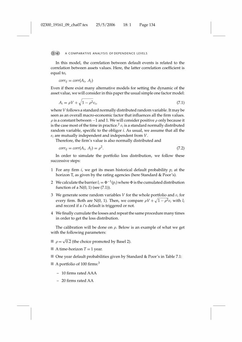
Figure 7.4 Histogram of the losses in the multi-factor intensity-basedmodel (T = 1 year)

first model. We just have to draw the realizations of additional gamma ran-dom variables (one for each obligor). In practice, there are now two freeparameters α0 and αi, related to Z0 and Zi respectively. This may causesome estimation complications, even if the log-likelihood of the observa-tions can be written in closed form (Parner, 1998). In Figure 7.4, we drawthe histogram of the losses obtained with model (7.10). Since we imposethat the expectation of the global frailty component Z0 + Zi equals one,we draw Z0 ∼ G(α0, α0 + α) and Z0 ∼ G(α, α0 + α). We have chosen theparameter values α0 = 0.5 and α = 0.5 for every i in Figure 7.4.

In this case,

Var(Z0 + Zi) = α0/(α0 + α)2 + α/(α0 + α)2 = 1

and the correlated frailty Z0 + Zi has the same two first moments as inFigure 7.2. The loss distributions seem to be very similar. At first glance,the introduction of specific components does not lessen too much thedependence between defaults.9

02300_19161_09_cha07.tex 25/5/2006 18: 1 Page 145


80

500

1000

1500

60� �1 �0

�1

�0�1

�0�1

�0�1

40 20 20 406080

0

Var

80

600

1200

1800

60� �1

40 20 20 406080

0

Evar

80

48

1216

2024

24

68

1012

60� �1

40 20 20 406080

0

Kurtosis

80 60� �1

40 20 20 406080

0

Mean correlation(Z)

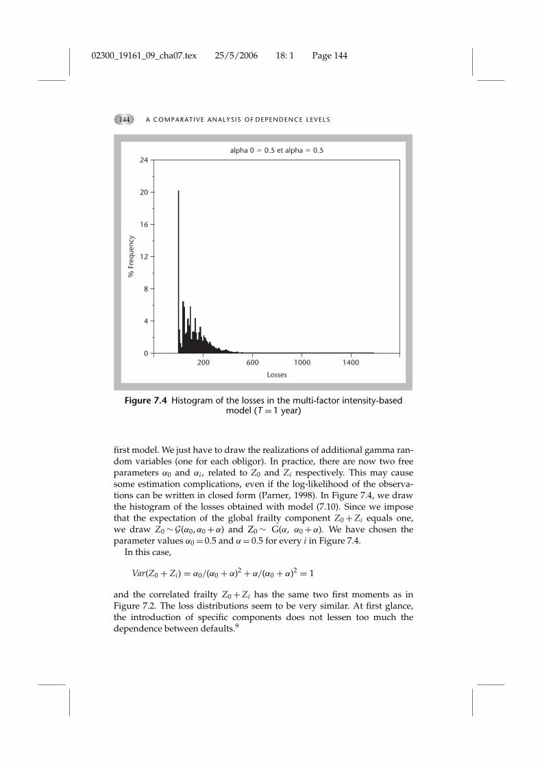
Figure 7.5 Combined effect of the parameters α0 and α in the multi-factorintensity model

We lead many simulations with different values of the parameters α0and αi in order to study their combined effects on the loss distribution (seeFigure 7.5).

The variance of Z0 + Zi varies from 0.005 to 50 when (α0, α) varies from0.01 to 100, which seems to be reasonable. The levels of our dependenceindicators seem to be in line with those obtained in section 7.3. Note that welose some dependence when the relative importance between Z0 and Zi isbalanced. This is due to a diversification effect inside both components of thefrailty factors. Globally, adding an idiosyncratic frailty allow more flexibilityin the model, without losing the ability to reach realistic dependence levels.

02300_19161_09_cha07.tex 25/5/2006 18: 1 Page 146


Actually, the ratio r = α/α0 provides a good measure of the dependence weobtain: the larger r, the higher the dependence indicators.

7.5.2 α-stable distributions

Properties of the family

Stable distributions allow building a rich class of probability distributions.They induce highly skewed and heavy tails features and have many interest-ing mathematical properties: see the survey of Samorodnitsky and Taqqu(1994), Hougaard (1986), or Mittnik and Rachev (1999) and Carr and Wu(2002) for financial applications. However, the lack of closed-form formu-las for their densities and their cumulative distribution functions, despitea few exceptions, has been a major drawback that has limited their use bypractitioners. To correct the ideas, we recall some basic theoretical resultsconcerning such distributions.

Definition 1 A random variable X is said to be α-stable if for any X1 andX2, some independent copies of X, and for any positive numbers c1 andc2, there exist c ∈ R

+ and d ∈ R such that:

cX + dd= c1X1 + c2X2

If d = 0, X is said to be strictly stable.

There are other equivalent definitions of α-stable distributions (see Nolan,2004, for a more detailed presentation of this distribution family) and weare going to invoke the following one because it is much more tractable:

Definition 2 Arandom variable X is said to be α-stable if its characteristicfunction takes the form:

�X(t)def= E(eitX) =

{exp(−γα |t|α (1 − iβ tan

(πα2

)sign(t)) + iδt) if α �= 1,

exp(−γ |t| (1 + iβ 2π

sign(t) ln (|t|)) + iδt) if α = 1,

(7.11)

where α ∈ [0, 2], β ∈ [−1, 1], γ ≥ 0 and δ ∈ R.

This definition shows that an α-stable distribution generally requires fourparameters as inputs:

� α, the index of stability. It is related to the tail behavior of the distribution.The smaller α, the stronger the leptokurtic feature of the distribution.

� β, the skewness parameter. If β = 0 then the distribution is symmetrical.If β > 0 then it is right skewed. Otherwise, it is left skewed.

� γ , the scale parameter.

02300_19161_09_cha07.tex 25/5/2006 18: 1 Page 147


� δ, the location parameter (When α > 1, it measures the mean of thedistribution).

There are multiple parameterizations for α-stable laws which may lead tosome confusion. We keep the previous one, and we denote the α-stabledistribution by S(α, β, γ , δ) and its probability distribution function by f .

Definition 3 The support of an α-stable distribution is:

support ( f (x)) =

⎧⎪⎨⎪⎩

[δ, +∞] if α < 1 and β = 1,

[−∞, δ] if α < 1 and β = −1,

R otherwise.

(7.12)

Because of the presence of heavy tails, all moments do not exist. Actually,we have:

Definition 4 Let X ∼ S(α, β, γ , δ).

E(|X|r) < +∞ if and only if 0 < r < α.

As far as we are concerned, for example, within the framework of frailtymodels the Laplace transforms are key tools.

Definition 5 Let X ∼ S(α, β, γ , δ). Its Laplace transform is defined if andonly if β = 1, in which case it equals:

LX(t) ≡ E(

e−tX)

=exp(−tδ − tαγα sec

(πα

2

)), t ≥ 0, (7.13)

by denoting sec(x) = 1/cos(x).We will also need the following property:

Definition 6 Let X ∼ S(α, β, γ , δ) where α �= 1. Then for all α �= 0 andb ∈ R we have aX + b ∼ S(α, sign(a) β, |a|γ , aδ + b).

In particular, if Z ∼ S(α, β, 1, 0) and

X ={

γZ + δ if α �= 1,

γZ + (δ + 2βπ

γ ln (γ)) if α = 1,

then X ∼ S(α, β, γ , δ). We will simply note S(α, β) instead of S(α, β, 1, 0).Thus, by some linear transformations, we get all the α-stable laws startingfrom the family S(α, β).

7.5.3 Simulation of an α-stable distribution

As mentioned earlier, α-stable density functions do not admit closed forms.The usual method to obtain these functions is to inverse their character-istic functions f (x) = 1

2π

∫exp(−itx)�X(t) dt. Except in a few cases,10 the

estimation of the latter expression is difficult, and will rather use the method

02300_19161_09_cha07.tex 25/5/2006 18: 1 Page 148


in Chambers, Mallows and Stuck (1996). Let W be a random variableexponentially distributed with parameter λ = 1, and U a random variableuniformly distributed on [−π

2 , π2 ] and let ξ = arctan(β tan(πα/2))/α and the

random variable

Z =

⎧⎪⎪⎪⎪⎪⎪⎪⎨⎪⎪⎪⎪⎪⎪⎪⎩

sin (α(ξ + U))α√

cos (αξ) cos (U)

(cos (αξ + (α − 1)U)

W

)1 − α

α , if α �= 1

2π

⎛⎜⎝(π

2+ βU

)tan (U) − β ln

⎛⎜⎝ π

2 W cos Uπ

2+ βU

⎞⎟⎠

⎞⎟⎠ , if α = 1.

(7.14)

Then Z ∼ S(α, β). To get S(α, β, γ , δ), we invoke the linear transform ofDefinition 6.

7.5.4 α-stable intensity-based model

To simulate more heavy tailed random intensities, we are going to replacethe gamma frailty random variable in (7.3) by an α-stable distributed frailty.As an intensity process is always positive and according to (7.12), we imposethat α < 1, β = 1 and δ = 0 in order that the support of the frailty is [0, +∞].We keep the same simple specification as in our first intensity model: forevery obligor i and every time t,

λi(t) = λi = Zλ0,i

Therefore, Z ∼ S(α, 1, γ ,0) where α ∈ [0, 1]. Indeed, as the frailty variable hasa multiplicative effect on the intensity, its baseline hazard function playsthe role of a scale parameter. Thus, the parameter γ is unnecessary. In fact,we identify λ0,i by using the Laplace transform of the α-stable distribution(7.13), which leads to the one-year default probability:

pi = 1 −exp(−γα sec

(πα

2

)γα λα

0,i

)This implies:

λ0 = 1γ

⎛⎝ ln

(1

1−pi

)sec

(πα2

)⎞⎠

1α

Hence

λd= λ0Z

= 1γ

⎛⎝ ln

(1

1−pi

)sec

(πα2

)⎞⎠

1α

γS(α, 1) (7.15)

=⎛⎝ ln

(1

1−pi

)sec(πα

2 )

⎞⎠

1α

S(α, 1)

02300_19161_09_cha07.tex 25/5/2006 18: 1 Page 149


2000

4

8

12

16

20

24

600 1000 1400

Losses

alpha � 0.8%

Fre

que

ncy

Figure 7.6 Histogram of the losses in the α – stable intensity based model

Obviously, the random intensities, and so the whole model, depend onα. In order to simulate the loss distribution, we draw a random variableZ ∼ S(α,1) (see (7.14)) and we deduce λ from (7.15). We then follow the samesteps as with the other models. For example, setting α = 0.8 we obtain thehistogram of portfolio11 losses in Figure 7.6.

As expected, it is now easier to get large dependence levels betweenindividual defaults inside the portfolio. Actually, the correlation betweendefault events is even stronger than in our previous Merton-type model.Thus, α-stable frailties are a simple way to induce a strongly dependentcredit-risky portfolio.

Table 7.6 presents the characteristics of the distribution for different valuesof the parameter α. The smaller the α, the larger the dependence betweendefault events. The dependence indicators we get with α-stable laws arestronger than previously. Thus, it is a relatively simple way to generatehighly dependent defaults, without modifying the intensity-based frame-work. Surprisingly, the kurtosis is increasing when the VaR and ExpectedShortfall are decreasing. This can be explained by a type of degeneracy ofthe loss distributions: when α is very small, the losses are concentratednear the origin and very far towards the right. The implicit reference to the

02300_19161_09_cha07.tex 25/5/2006 18: 1 Page 150


Table 7.6 α-stable intensity-based model, T = 1 year

α 0.1 0.3 0.5 0.7 0.8 0.9 0.95

Quantile of order 99% 1588 1416 1170 1108 990 663 505

E(losses | losses > q99%) 2048 1905 1766 1654 1510 1066 844

Skewness 5.33 5.22 5.51 6.81 6.98 6.74 7.07

k kurtosis 45.59 46.10 51.11 87.51 90.26 95.60 115.48

Average correlation (%) 44.33 40.19 33.72 23.86 17.26 9.35 4.86

Gaussian distribution (when dealing with kurtosis) has no more sense insuch situations.

7.6 CONCLUSION

We find some evidence that realistic and comparable dependence levelscan be obtained by both intensity-style models and Merton-style models.With long time horizons, the latter approach gains a relative advantage, butthe former can be strengthened by some extensions towards α-stable frailtymodels. Thus, the issue is not really to choose between both approaches butrather to specify conveniently a model, an intensity-based one or a Merton-style one. In practice, it is important to solve the following issues:

� What is the correlation scope that the model needs to cover?

� Observable and/or unobservable exogenous factors?

� Which distribution for such factors?

� Constant or time dependent frailties? If yes, whose process is best suited?

Moreover, one of the main practical issues concerns the estimation of thekey dependence parameters, typically ρ and α in our previous frameworks.Such an issue may become a hurdle for the implementation of such models.For instance, clean estimations of the simplistic frailty model (7.3) are farfrom trivial (see Andersen, Gill, Borgan and Keiding, 1997, for the theory,and Metayer, 2004, for a financial application). And, even more, the intro-duction of dynamic frailties12 induces likelihoods without any closed form,which imposes some delicate numerical optimization procedures (simulatedmaximum likelihood, EM algorithm, and so for).

APPENDIX A: CALCULATION OF CORRELATION BETWEENDEFAULT EVENTS

Our goal is the calculation of the correlation between default events and between the datest = 0 and t = T, controlling eventually by the rating categories. Technically speaking, it isequivalent to the calculation of joint default probabilities.

02300_19161_09_cha07.tex 25/5/2006 18: 1 Page 151

JEAN-DAV ID FERMANIAN AND MOHAMMED SBA I 151

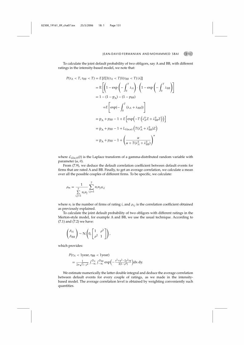
To calculate the joint default probability of two obligors, say A and BB, with differentratings in the intensity-based model, we note that:

P(τA < T, τBB < T) = E [E[1(τA < T)1(τBB < T) |λ]]

= E

[(1 − exp

(−

∫ T

0λA

)·(

1 − exp

(−

∫ T

0λBB

)]

= 1 − (1 − pA) − (1 − pBB)

+E

[exp(−

∫ T

0(λA + λBB))

]

= pA + pBB − 1 + E[exp

(−T

(λ0

AZ + λ0BBZ

))]

= pA + pBB − 1 + LG(α,α)

(T(λ0

A + λ0BB)Z

)

= pA + pBB − 1 +(

α

α + T(λ0A + λ0

BB)

)α

where LG(α,θ)(t) is the Laplace transform of a gamma-distributed random variable withparameter (α, θ).

From (7.9), we deduce the default correlation coefficient between default events forfirms that are rated A and BB. Finally, to get an average correlation, we calculate a meanover all the possible couples of different firms. To be specific, we calculate:

ρm = 17∑

i,j=1ninj

7∑i,j=1

ninjρi,j

where ni is the number of firms of rating i, and ρi,j is the correlation coefficient obtainedas previously explained.

To calculate the joint default probability of two obligors with different ratings in theMerton-style model, for example A and BB, we use the usual technique. According to(7.1) and (7.2) we have:

(AA

ABB

)∼ N

(0,

[1

ρ2

ρ2

1

]),

which provides:

P(τA < 1year, τBB < 1year)

= 12π

√1−ρ4

∫ DA−∞

∫ DBB−∞ exp

(− x2+y2−2ρ2xy

2(1−ρ4)

)dx dy.

We estimate numerically the latter double integral and deduce the average correlationbetween default events for every couple of ratings, as we made in the intensity-based model. The average correlation level is obtained by weighting conveniently suchquantities.

02300_19161_09_cha07.tex 25/5/2006 18: 1 Page 152


APPENDIX B: EXTENSIONS OF THE RESULTS TO LARGE TIMEHORIZONS

We use the same method as in sections 7.2 and 7.3. We choose the following defaultprobabilities:

Average default rates over 1981–2002

Rating CCC B BB BBB A AA AAA

PD (%) (5 years) 61.35 33.02 14.45 3.83 0.75 0.27 0,11

PD (%) (20 years) 73.94 67.68 48.09 19.48 6.78 4.38 1.13

Source: Standard & Poor’s Credit Pro.

We obtain default event correlations for the time horizons T = 5 years and T = 20years (Tables 7.7, 7.8, 7.10 and 7.11), and the usual dependence indicators with T = 10years (Tables 7.9 and 7.12). In the latter case, particularly, the scope of values obtained inboth cases is similar.

Note that when the time horizon T is increasing, it is surely questionable to assume thesame values ρ and α as when T = 1 year apply. Indeed, in the Merton-style models thereis some empirical evidence that the asset correlations depend on T (see the discussion inde Servigny and Renault, 2002, for example).

Moreover, since we assumed the random default intensities λi are constant func-tions between 0 and T, their (random) levels should be less and less variable when T isincreasing.13 It should be more relevant to simulate an annual process (Zt) for the frailty,but this does not belong in our simple framework. Thus, a realistic range of α-values is

Table 7.7 5-years default events correlations in the Merton model, with ρ = √0.2 (%)


AAA 0.63 0.82 1.10 1.59 1.89 1.85 1.51

AA 0.82 1.10 1.48 2.21 2.68 2.67 2.22

A 1.10 1.48 2.04 3.12 3.90 3.98 3.40

BBB 1.59 2.21 3.12 5.05 6.67 7.11 6.37

BB 1.89 2.68 3.90 6.67 9.32 10.43 9.84

B 1.85 2.67 3.98 7.12 10.43 12.15 12.01

CCC 1.51 2.22 3.40 6.37 9.84 12.01 12.53

Table 7.8 20-years default events correlations in the Merton model, with ρ = √0.2 (%).


AAA 2.60 3.68 4.02 4.64 4.41 3.78 3.50

AA 3.68 5.41 6.01 7.22 7.20 6.35 5.92

A 4.02 6.01 6.70 8.17 8.30 7.40 6.93

BBB 4.64 7.22 8.17 10.41 11.16 10.27 9.73

BB 4.41 7.20 8.30 11.16 12.81 12.28 11.81

B 3.78 6.35 7.40 10.27 12.28 12.09 11.74

CCC 3.50 5.92 6.93 9.73 11.81 11.74 11.43

02300_19161_09_cha07.tex 25/5/2006 18: 1 Page 153

153

Table 7.9 10-years Merton model

ρ 0.01 0.1 0.3 0.4 0.6 0.7 0.9 0.95

Q99% quantile of order 99% 1,193 1,254 1,543 1,827 2,357 2,664 3,537 3,757

E(losses | losses > q99%) 1,253 1,339 1,663 2,020 2,704 3,089 4,145 4,426

skewness 0.15 0.22 0.46 0.75 1.05 1.20 1.53 1.5

k kurtosis 2.95 3.08 3.15 3.68 4.50 4.78 5.87 6.42

average correlation (%) 10"3 0.24 2.26 4.19 10.62 15.62 31.60 37.72

Table 7.10 5-years default events correlations in the intensity model,with α = 1 (%)


AAA 0.04 0.05 0.08 0.16 0.30 0.36 0.31

AA 0.05 0.08 0.12 0.24 0.44 0.55 0.53

A 0.08 0.12 0.18 0.39 0.71 0.93 0.94

BBB 0.16 0.24 0.39 0.84 1.57 2.14 2.22

BB 0.30 0.44 0.71 1.57 3.02 4.19 4.31

B 0.36 0.55 0.93 2.14 4.19 6.24 7.34

CCC 0.31 0.53 0.94 2.22 4.31 7.34 13.01

Table 7.11 20-years default events correlations in the intensity model,with α = 1 (%)


AAA 0.13 0.07 0.12 0.23 0.29 0.33 0.26

AA 0.07 0.49 0.44 0.57 1.10 0.93 0.27

A 0.12 0.44 0.48 0.67 1.07 1.02 0.47

BBB 0.23 0.57 0.67 1.06 1.59 1.65 1.11

BB 0.29 1.10 1.07 1.59 3.03 2.99 2.04

B 0.33 0.93 1.02 1.65 2.99 3.46 3.41

CCC 0.26 0.27 0.47 1.11 2.04 3.41 8.39

Table 7.12 10-years intensity-based model

Var(Z) = 1/α 0.01 0.1 0.5 2 5 10 50 100

quantile of order 99% 1190 1209 1283 1508 1766 2015 2722 3026

E(losses | losses > q99%) 1256 1275 1364 1621 1897 2178 3003 3333

skewness 0.16 0.14 0.15 0.31 0.41 0.52 0.87 0.99

k kurtosis 2.99 2.98 2.96 2.89 2.72 2.63 2.87 3.16

average correlation (%) 0.01 0.09 0.44 1.68 3.82 6.72 18.24 24.17

02300_19161_09_cha07.tex 25/5/2006 18: 1 Page 154


becoming thinner and thinner when the time horizon is growing. That is why a straightcomparison between Tables 7.8 and 7.11 particularly is not fully satisfying, because α = 1is probably too high is such a case.

NOTES

1. See Luciano (2004) for a discussion in the finance field. In a more general context,there is no issue to rewrite the marginal laws of the default times with intensities. Atthe opposite, it is more challenging to rewrite the full joint law of defaults because oneneeds to invoke multivariate hazard rates (Dabrowska, 1988; Fermanian, 1997). Forexample, a large number of intensities has to be modelized: 2m − 1 when m denotesthe number of firms in the portfolio. In practice, such a number is unrealistic whendealing with more than 2 or 3 obligors.

2. Even if some firms or more generally some industries may be considered as neg-atively correlated with the “market”, or rather with the vast majority of othercorporates.

3. Since most of bank portfolios are composed mainly with investment grade debts, weoverweight such firms.

4. The recovery rate is assumed to be zero here. This is not a limitation of our purpose.Indeed, in this chapter we do not try to study the internal source of randomnessgiven by the exposure amounts.

5. Particularly Hull and White (2001), Schönbucher and Schubert (2003).6. A random intensity model with constant levels between 0 and T and the same frailty

for all obligors.7. The relative sizes of the monthly default rates in Figure 7.3 are comparable with

annual default rates because the former are trailed over 12 months.8. The unobservable explanatory variables that are specific to i and that have not been

taken into account previously in the vector Xi.9. At least when we keep the balance between both Z0 and Zi.

10. For example, α = 2 provides a Gaussian law and α = 1, β = 0 provides a Cauchydistribution.

11. We are always dealing with the same portfolio from the beginning.12. Paik et al. (1994) or Yue and Chan (1997), for instance.13. because such λi are comparable with mean monthly default rates over a period T.

REFERENCES

Andersen, P.K., Gill, R., Borgan, O. and Keiding, N. (1997) Statistical Models Based onCounting Processes (New York: Springer).

Carr, P. and Wu, L. (2002) “The Finite Moment Log Stable Process and Option Pricing”,Working Paper.

Chambers, J.M., Mallows, C.L. and Stuck, B.W. (1976) “A Method for Simulating StableRandom Variables”, Journal of the American Statistical Association, 71(2): 340–4.

Clayton, D. and Cuzick, J. (1985) “Multivariate Generalizations of the ProportionalHazards Model”, Journal of the Royal Statistical Society, A, 148(1): 82–117.

Crouhy, M., Galai, D. and Mark, R. (2000) “A Comparative Analysis of Current CreditRisk Models”, Journal of Banking and Finance, 24(1–2): 59–117.

Dabrowska, D. (1988) “Kaplan–Meier on the Plane”, Annals of Statistics, 16(4): 1475–89.Das, S., Freed, L., Geng, G. and Kapadia, N. (2002) “Correlated Default Risk”, Working

Paper.

02300_19161_09_cha07.tex 25/5/2006 18: 1 Page 155


Duffie, D. and Singleton, K. (1999) “Modeling Term Structure of Defaultable Bonds”,Review of Financial Studies, 12(4): 687–720.

Elizalde, A. (2003) “Credit Risk Models I: Default Correlation in Intensity Models”,Working Paper CEMFI.

Fermanian, J.D. (1997) “Multivariate Hazard Rates Under Random Censorship”, Journalof Multivariate Analysis, 62(2): 273–309.

Frey, R. and McNeil, A. (2001) Modelling Dependent Defaults. ETH E-collection.Hougaard, P. (1986) “Survival Models for Heterogeneous Populations Derived from

Stable Distributions”, Biometrika, 73(2): 387–96.Hougaard, P. (2000) Analysis of Multivariate Survival Data (New York, NY: Statistics for

Biology and Health, Springer).Hull, J. and White, A. (2001) “Valuing Credit Default Swaps II: Modeling Default

Correlations”, Journal of Derivatives, 8(3): 12–22.Jarrow, R., Lando, D. and Turnbull, S. (1997) “A Markov Model for the Term Structure of

Credit Risk Spreads”, Review of Financial Studies, 10(3): 481–523.Koyluoglu, H. and Hickman, A. (1998) “A Generalized Framework for Credit Risk

Portfolio Models”, Working Paper.Luciano, E. (2004) “Credit Risk Assessment via Copulas: Association In-Variance and

Risk-Neutrality”, Working Paper, University of Turin, Italy.Metayer, B. (2005) “Shared Frailty Model for Rating Transitions”, Working Paper.Mittnik, S. and Rachev, S.T. (1999) Stable Models in Finance (New York, NY: John Wiley &

Sons).Nolan, J.P. (2004) “Stable Distributions: Models for Heavy Tailed Data” Working Paper,

American University, Washington, DC.Nyfeler, M. (2000) “Modeling Dependencies in Credit Risk Management”, Thesis, ETH,

Zürich.Paik, M.C., Tsai, W. and Ottman, R. (1994) “Multivariate Survival Analysis Using

Piecewise Gamma Frailty”, Biometrics, 50(4): 975–88.Parner, E. (1998) “Asymptotic Theory for the Correlated Gamma-Frailty Model”, Annals

of Statistics, 26(1): 183–214.Samorodnitsky, G. and Taqqu, M.S. (1994) Stable Non-Gaussian Random Variables (New

York, NY: Chapman and Hall).Schlögl, E. (2002) “Default Correlation Modeling”, Working Paper, University of

Technology Sydney, Australia.Schönbucher, P.J. (2001) “Factor Models for Portfolio Credit Risk”, Bonn Economics

Discussion Paper, No. 16.Schönbucher, P.J. (2003) Credit Derivatives Pricing Models: Models, Pricing and Implementa-

tion (New York, NY: John Wiley & Sons).Schönbucher, P.J. and Schubert, D. (2001) “Copula-Dependent Default Risk in Intensity

Models”, Working Paper.de Servigny, A. and Renault, O. (2002) “Default Correlation: Empirical Results”, Working

Paper, Standard and Poor’s solutions.Standard & Poor’s (2003) Special Report. Rating performances 2002. Février 2003.Turnbull, S. (2003) “Practical Issues in Modeling Default Dependence”, Working Paper,

Houston.Yashin, A.I. and Iachine, I.A. (1995) “Genetic Analysis of Durations: Correlated Frailty

Model Applied to Survival of Danish Twins”, Genetic Epidemiology, 12(3): 529–38.Yu, F. (2003) “Dependent Default in Intensity-based Models” Working Paper, University

of California, Irvine.Yue, H. and Chan, K.S. (1997) “A Dynamic Frailty Model for Multivariate Survival Data”,

Biometrics, 53(3): 785–93.

Documents

CHAPTER 7 A Comparative Analysis of Dependence Levels in