Comparative Analysis of Neural Network Models for

Premises Valuation Using SAS Enterprise Miner

Tadeusz Lasota1, Michał Makos2, Bogdan Trawiński2,

1 Wrocław University of Environmental and Life Sciences, Dept. of Spatial Management

Ul. Norwida 25/27, 50-375 Wroclaw, Poland 2 Wrocław University of Technology, Institute of Informatics,

Wybrzeże Wyspiańskiego 27, 50-370 Wrocław, Poland

Tadeusz.Lasota@wp.pl, Michal.Makos@gmail.com, Bogdan.Trawinski@pwr.wroc.pl

Abstract. The experiments aimed to compare machine learning algorithms to

create models for the valuation of residential premises were conducted using the

SAS Enterprise Miner 5.3. Eight different algorithms were used including

artificial neural networks, statistical regression and decision trees. All models

were applied to actual data sets derived from the cadastral system and the

registry of real estate transactions. A dozen of predictive accuracy measures

were employed. The results proved the usefulness of majority of algorithms to

build the real estate valuation models.

Keywords: neural networks, real estate appraisal, AVM, SAS Enterprise Miner

1 Introduction

Automated valuation models (AVMs) are computer programs that enhance the

process of real estate value appraisal. AVMs are currently based on methodologies

from multiple regression analysis to neural networks and expert systems [11]. The

quality of AVMs may vary depending on data preparation, sample size and their

design, that is why they must be reviewed to determine if their outputs are accurate

and reliable. A lot need to be done to create a good AVM. Professional appraisers

instead of seeing in AVMs a threat should use them to enhance services they provide.

Artificial neural networks are commonly used to evaluate real estate values. Some

studies described their superiority over other methods [1], [7]. Other studies pointed

out that ANN was not the “state-of-the-art” tool in that matter [13] or that results

depended on data sample size [9]. Studies showed that there is no perfect

methodology for real estate value estimation and mean absolute percentage error

ranged from almost 4% to 15% in better tuned models [4] .

In our pervious works [3], [5], [6] we investigated different machine learning

algorithms, among others genetic fuzzy systems devoted to build data driven models

to assist with real estate appraisals using MATLAB and KEEL tools. In this paper we

report the results of experiments conducted with SAS Enterprise Miner aimed at the

comparison of several artificial neural network and regression methods with respect to

a dozen performance measures, using actual data taken from cadastral system in order

to assess their appropriateness to an internet expert system assisting appraisers’ work.

2 Cadastral Systems as the Source Base for Model Generation

The concept of a data driven models for premises valuation, presented in the paper,

was developed on the basis of the sales comparison method. It was assumed that

whole appraisal area, which means the area of a city or a district, is split into sections

(e.g. clusters) of comparable property attributes. The architecture of the proposed

system is shown in Fig. 1. The appraiser accesses the system through the internet and

chooses an appropriate section and input the values of the attributes of the premises

being evaluated into the system, which calculates the output using a given model. The

final result as a suggested value of the property is sent back to the appraiser.

Fig. 1. Information systems to assist with real estate appraisals

Actual data used to generate and learn appraisal models came from the cadastral

system and the registry of real estate transactions referring to residential premises sold

in one of big Polish cities at market prices within two years 2001 and 2002. They

constituted original data set of 1098 cases of sales/purchase transactions. Four

attributes were pointed out as price drivers: usable area of premises, floor on which

premises were located, year of building construction, number of storeys in the

building, in turn, price of premises was the output variable.

3 SAS Enterprise Miner as the Tool for Model Exploration

SAS Enterprise Miner 5.3 is a part of SAS Software, a very powerful information

delivery system for accessing, managing, analyzing, and presenting data [8], [10].

SAS Enterprise Miner has been developed to support the entire data mining process

from data manipulation to classifications and predictions. It provides tools divided

into five fundamental categories:

Sample. Allows to manipulate large data sets: filter observation, divide and merge

data etc.

Explore. Provides different tools that can be very useful to get to know the data by

viewing observations, their distribution and density, performing clustering and

variable selection, checking variable associations etc.

Modify. That set of capabilities can modify observations, transform variables, add

new variables and handle missing values etc.

Model. Provides several classification and prediction algorithms such as neural

network, regression, decision tree etc.

Assess. Allows to compare created models.

SAS Enterprise Miner allows for batch processing which is a SAS macro-based

interface to the Enterprise Miner client/server environment. Batch processing supports

the building, running, and reporting of Enterprise Miner 5 process flow diagrams. It

can be run without the Enterprise Miner graphical user interface (GUI). User-friendly

GUI enables designing experiments by joining individual nodes with specific

functionality into whole process flow diagram. The graph of the experiments reported

in the present paper is shown in Fig. 2.

Following SAS Enterprise Miner algorithms for building, learning and tuning data

driven models were used to carry out the experiments (see Table 1):

Table 1. SAS Enterprise Miner machine learning algorithms used in study.

Type Code Descritption

Neural

networks

MLP Multilayer Perceptron

AUT AutoNeural

RBF Ordinary Radial Basis Function with Equal Widths

DMN DMNeural

Statistical

regression

REG Regression

DMR Dmine Regression

PLS Partial Least Square

Decision

trees

DTR

Decision Tree (CHAID, CART, and C4.5)

MLP - Neural Network. Multilayer Perceptron is the most popular form of neural

network architecture. Typical MLP consists of input layer, any number of hidden

layers with any number of units and output layer. It usually uses sigmoid activation

function in the hidden layers and linear combination function in the hidden and output

layers. MLP has connections between the input layer and the first hidden layer,

between the hidden layers, and between the last hidden layer and the output layer.

AUT - AutoNeural. AutoNeural node performs automatic configuration of neural

network Multilayer Perceptron model. It conducts limited searches for a better

network configuration.

RBF - Neural Network with ORBFEQ i.e. ordinary radial basis function with

equal widths. Typical radial neural network consists of: input layer, one hidden layer

and output layer. RBF uses radial combination function in the hidden layer, based on

the squared Euclidean distance between the input vector and the weight vector. It uses

the exponential activation function and instead of MLP’s bias, RBFs have a width

associated with each hidden unit or with the entire hidden layer. RBF has connections

between the input layer and the hidden layer, and between the hidden layer and the

output layer.

DMN - DMNeural. The DMNeural node enables to fit an additive nonlinear

model that uses the bucketed principal components as inputs. The algorithm was

developed to overcome the problems of the common neural networks that are likely to

occur especially when the data set contains highly collinear variables. In each stage of

the DMNeural training process, the training data set is fitted with eight separate

activation functions. The algorithm selects the one that yields the best results. The

optimization with each of these activation functions is processed independently.

REG - Regression: Linear or Logistic. Linear regression method is a standard

statistical approach to build a linear model predicting a value of the variable while

knowing the values of the other variables. It uses least mean square in order to adjust

the parameters of the linear model/function. Enables usage of the stepwise, forward,

and backward selection methods. Logistic regression is a standard statistical approach

to build a logistic model predicting a value of the variable while knowing the values

of the other variables. It uses least mean square in order to adjust the parameters of

the quadratic model/function. Enables usage of the stepwise, forward, and backward

selection methods.

PLS - Partial Least Squares. Partial least squares regression is an extension of the

multiple linear regression model. It is not bound by the restrictions of discriminant

analysis, canonical correlation, or principal components analysis. It uses prediction

functions that are comprised of factors that are extracted from the Y'XX'Y matrix.

DMR - Dmine Regression. Computes a forward stepwise least-squares regression.

In each step, an independent variable is selected that contributes maximally to the

model R-square value.

DTR - Decision Tree. An empirical tree represents a segmentation of the data that

is created by applying a series of simple rules. Each rule assigns an observation to a

segment based on the value of one input. One rule is applied after another, resulting in

a hierarchy of segments within segments. It uses popular decision tree algorithms

such as CHAID, CART, and C4.5. The node supports both automatic and interactive

training. Automatic mode automatically ranks the input variables, based on the

strength of their contribution to the tree. This ranking can be used to select variables

for use in subsequent modeling.

4 Experiment Description

The main goal of the study was to carry out comparative analysis of different neural

network algorithms implemented in SAS Enterprise Miner and use them to create and

learn data driven models for premises property valuation with respect to a dozen of

performance measures. Predictive accuracy of neural network models was also

compared with a few other machine learning methods including linear regression,

decision trees and partial least squares regression. Schema of the experiments

comprising algorithms with preselected parameters is depicted in Fig. 2.

Fig. 2. Schema of the experiments with SAS Enterprise Miner

The set of observations, i.e. the set of actual sales/purchase transactions containing

1098 cases, was clustered and then partitioned into training and testing sets. The

training set contained 80% of data from each cluster, and training one – 20%, that is

871 and 227 observations respectively. As fitness function the mean squared error

(MSE) was applied to train models. A series of initial tests in order to find optimal

parameters of individual algorithms was accomplished. Due to lacking mechanism of

cross validation in any Enterprise Miner modeling nodes, each test was performed 4

times (with different data partition seed) and the average MSE was calculated.

In final stage, after the best parameters set for each algorithm were determined,

a dozen of commonly used performance measures [2], [12] were applied to evaluate

models built by respective algorithms. These measures are listed in Table 2 and

expressed in the form of following formulas below, where yi denotes actual price and

𝑦 i – predicted price of i-th case, avg(v), var(v), std(v) – average, variance, and

standard deviation of variables v1,v2,…,vN, respectively and N – number of cases in the

testing set.

Table 2. Performance measures used in study

Denot. Description Dimen-

sion

Min

value

Max

value

Desirable

outcome

No. of

form.

MSE Mean squared error d2 0 ∞ min 1

RMSE Root mean squared error d 0 ∞ min 2

RSE Relative squared error no 0 ∞ min 3

RRSE Root relative squared error no 0 ∞ min 4

MAE Mean absolute error d 0 ∞ min 5

RAE Relative absolute error no 0 ∞ min 6

MAPE Mean absolute percentage

error

% 0 ∞ min 7

NDEI Non-dimensional error index no 0 ∞ min 8

r Linear correlation coefficient no -1 1 close to 1 9

R2 Coefficient of determination % 0 ∞ close to 100% 10

var(AE) Variance of absolute errors d2 0 ∞ min 11

var(APE) Variance of absolute

percentage errors

no 0 ∞ min 12

𝑀𝑆𝐸 =1

𝑁 𝑦𝑖 − 𝑦 𝑖

2𝑁

𝑖=1 (1)

𝑅𝑀𝑆𝐸 = 1

𝑁 𝑦𝑖 − 𝑦 𝑖

2𝑁

𝑖=1 (2)

𝑅𝑆𝐸 = 𝑦𝑖 − 𝑦 𝑖

2𝑁𝑖=1

𝑦𝑖 − 𝑎𝑣𝑔(𝑦) 2𝑁𝑖=1

(3)

𝑅𝑅𝑆𝐸 = 𝑦𝑖 − 𝑦 𝑖

2𝑁𝑖=1

𝑦𝑖 − 𝑎𝑣𝑔(𝑦) 2𝑁𝑖=1

(4)

𝑀𝐴𝐸 =1

𝑁 𝑦𝑖 − 𝑦 𝑖

𝑁

𝑖=1 (5)

𝑅𝐴𝐸 = 𝑦𝑖 − 𝑦 𝑖

𝑁𝑖=1

𝑦𝑖 − 𝑎𝑣𝑔(𝑦) 𝑁𝑖=1

(6)

𝑀𝐴𝑃𝐸 =1

𝑁

𝑦𝑖 − 𝑦 𝑖

𝑦𝑖

𝑁

𝑖=1∗ 100% (7)

𝑁𝐷𝐸𝐼 =𝑅𝑀𝑆𝐸

𝑠𝑡𝑑(𝑦) (8)

𝑟 = 𝑦𝑖 − 𝑎𝑣𝑔(𝑦) 𝑁

𝑖=1 𝑦 𝑖 − 𝑎𝑣𝑔(𝑦 )

𝑦𝑖 − 𝑎𝑣𝑔(𝑦) 2𝑁𝑖=1 𝑦 𝑖 − 𝑎𝑣𝑔(𝑦 ) 2𝑁

𝑖=1

(9)

𝑅2 = 𝑦 𝑖 − 𝑎𝑣𝑔(𝑦) 2𝑁

𝑖=1

𝑦𝑖 − 𝑎𝑣𝑔(𝑦) 2𝑁𝑖=1

∗ 100% (10)

𝑣𝑎𝑟(𝐴𝐸) = 𝑣𝑎𝑟( 𝑦 − 𝑦 ) (11)

𝑣𝑎𝑟(𝐴𝑃𝐸) = 𝑣𝑎𝑟( 𝑦 − 𝑦

𝑦) (12)

5 Results of the Study

5.1 Preliminary Model Selection

Within each modeling class, i.e. neural networks, statistical regression, and decision

trees, preliminary parameter tuning was performed using trial and error method in

order to choose the algorithm producing the best models. All measures were

calculated for normalized values of output variables except for MAPE, where in order

to avoid the division by zero, actual and predicted prices had to be denormalized. The

nonparametric Wilcoxon signed-rank tests were used for three measures: MSE, MAE,

and MAPE. The algorithms with the best parameters chosen are listed in Table 3.

Table 3. Best algorithms within each algorithm class

Name Code Description

Neural Network:

MLP MLP

Training Technique: Trust-Region; Target Layer Combination

Fun: Linear; Target Layer Activation Fun: Linear; Target Layer

Error Fun: Normal; Hidden Units: 3

AutoNeural AUT Architecture: Block Layers; Termination: Overfitting; Number

of hidden units: 4

Neural Network:

ORBFEQ RBF

Training Technique: Trust-Region; Target Layer Combination

Fun: Linear; Target Layer Activation Fun: Identity; Target

Layer Error Fun: Entropy; Hidden Units: 30

DMNeural DMN Train activation function (selection): ACC; Train objective

function (optimization): SSE

Regression REG Regression Type: Linear; Selection Model: None

Dmine Regression DMR Stop R-Square: 0.001

Partial Least

Square PLS Regression model: PCR

Decision Tree DTR Subtree Method: N; Number of leaves: 16; p-value Inputs: Yes;

Number of Inputs: 3

5.2 Final Results

Final stage of the study contained comparison of algorithms listed in Table 3, using

all 12 performance measures enumerated in pervious section. The results of respective

measures for all models are shown in Fig. 3-14, it can be easily noticed that

relationship among individual models are very similar for some groups of measures.

Fig. 9 depicts that the values of MAPE range from 16.2% to 17.4%, except for PLS

with 18.9%, what can be regarded as fairly good, especially when you take into

account, that no all price drivers were available in our sources of experimental data.

Fig. 11 shows there is high correlation, i.e. greater than 0.8, between actual and

predicted prices for each model. In turn, Fig.12 illustrating the coefficients of

determination indicates that above 85% of total variation in the dependent variable

(prices) is explained by the model in the case of AUT and REG models and less than

60% for DMS and PLS models.

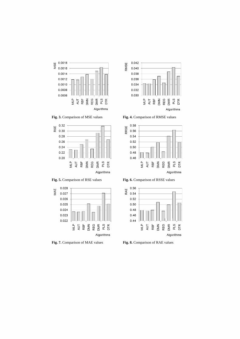
Fig. 3. Comparison of MSE values Fig. 4. Comparison of RMSE values

Fig. 5. Comparison of RSE values Fig. 6. Comparison of RSSE values

Fig. 7. Comparison of MAE values Fig. 8. Comparison of RAE values

Fig. 9. Comparison of MAPE values

Fig. 10. Comparison of NDEI values

Fig. 11. Comparison of correlation

coefficient (r) values

Fig. 12. Comparison of determination

coefficient (R2) values

Fig. 13. Comparison of var(AE) values Fig. 14. Comparison of var(APE) values

The nonparametric Wilcoxon signed-rank tests were carried out for three measures:

MSE, MAPE, and MAE. The results are shown in Tables 4, 5, and 6 in each cell

results for a given pair of models were placed, in upper halves of the tables – p-

values, and in lower halves final outcome, where N denotes that there are no

differences in mean values of respective errors, and Y indicates that there are

statistically significant differences between particular performance measures. In the

majority of cases Wilcoxon tests did not provide any significant difference between

models, except the models built by PLS algorithms, and REG with respect to MAPE.

Table 4. Results of Wilcoxon signed-rank test for squared errors comprised by MSE

MSE MLP AUT RBF DMN REG DMR PLS DTR

MLP

0.962 0.494 0.022 0.470 0.218 0.000 0.064

AUT N

0.758 0.180 0.650 0.244 0.001 0.114

RBF N N

0.284 0.924 0.271 0.001 0.035

DMN Y N N

0.426 0.942 0.000 0.780

REG N N N N

0.152 0.007 0.023

DMR N N N N N

0.002 0.176

PLS Y Y Y Y Y Y

0.097

DTR N N Y N Y N N

Table 5. Results of Wilcoxon test for absolute percentage errors comprised by MAPE

MAPE MLP AUT RBF DMN REG DMR PLS DTR

MLP

0.957 0.557 0.031 0.000 0.178 0.000 0.106

AUT N

0.854 0.102 0.000 0.372 0.001 0.143

RBF N N

0.088 0.000 0.180 0.000 0.067

DMN Y N N

0.000 0.392 0.001 0.977

REG Y Y Y Y

0.000 0.000 0.000

DMR N N N N Y

0.001 0.286

PLS Y Y Y Y Y Y

0.097

DTR N N N N Y N N

Table 6. Results of Wilcoxon signed-rank test for absolute errors comprised by MAE

MAE MLP AUT RBF DMN REG DMR PLS DTR

MLP

0.946 0.619 0.050 0.739 0.260 0.002 0.134

AUT N

0.692 0.145 0.934 0.306 0.001 0.135

RBF N N

0.178 0.799 0.195 0.001 0.091

DMN N N N

0.212 0.646 0.000 0.887

REG N N N N

0.166 0.004 0.059

DMR N N N N N

0.006 0.350

PLS Y Y Y Y Y Y

0.111

DTR N N N N N N N

Due to the non-decisive results of majority of statistical tests, rank positions of

individual algorithms were determined for each measure (see Table 7). Observing

median, average, minimal and maximal ranks it can be noticed that highest rank

positions gained AUT, MLP, REG, RBF algorithms and the lowest PLS and DMR.

Table 7 indicates also that some performance measures provide the same rank

positions, and two groups of those measures can be distinguished. First one based on

mean square errors contains MSE, RMSE, RSE, RRSE, NDEI, and the second one

based on mean absolute errors comprises MAE and RAE.

Table 7. Rank positions of algorithms with respect to performance measures (1 means the best)

MLP AUT RBF DMN REG DMR PLS DTR

MSE 2 1 4 5 3 7 8 6

RMSE 2 1 4 5 3 7 8 6

RSE 2 1 4 5 3 7 8 6

RRSE 2 1 4 5 3 7 8 6

MAE 3 2 4 7 1 5 8 6

RAE 3 2 4 7 1 5 8 6

MAPE 4 2 1 7 3 5 8 6

NDEI 2 1 4 5 3 7 8 6

r 3 1 4 6 2 7 8 5

R2 4 1 3 6 2 7 8 5

var(AE) 2 1 4 5 3 7 8 6

var(APE) 1 2 3 5 6 4 8 7

median 2.00 1.00 4.00 5.00 3.00 7.00 8.00 6.00

average 2.50 1.33 3.58 5.67 2.75 6.42 8.00 5.92

min 1 1 1 5 1 4 8 5

max 4 2 4 7 6 7 8 7

6 Conclusions and Future Work

The goal of experiments was to compare machine learning algorithms to create

models for the valuation of residential premises, implemented in SAS Enterprise

Miner 5.3. Four methods based on artificial neural networks, three different

regression techniques and decision tree were applied to actual data set derived from

cadastral system and the registry of real estate transactions.

The overall conclusion is that multilayer perceptron neural networks seem to

provide best results in estimating real estate value. Configuration of AutoNeural node

(which is actually implementation of MLP) gave a bit better results than MLP itself

almost in every error/statistical measure. The analysis of charts leads to a conclusion

that these eight algorithms can be divided into two groups with respect to their

performance. To the first group with better results belong: AutoNerual, Neural

Network: MLP, Linear Regression and Neural Network: ORBFEQ. In turn, to the

second group with worse outcome belong: Decision Tree, DMNeural, Partial Least

Squares and Dmine Regression.

Some performance measures provide the same distinction abilities of respective

models, thus it can be concluded that in order to compare a number of models it is not

necessary to employ all measures, but the representatives of different groups. Of

course the measures within groups differ in their interpretation, because some are

non-dimensional as well as in their sensitivity understood as the ability to show the

differences between algorithms more or less distinctly.

High correlation between actual and predicted prices was observed for each model

and the coefficients of determination ranged from 55% to 85% .

MAPE obtained in all tests ranged from 16% do 19%. This can be explained that

data derived from the cadastral system and the register of property values and prices

can cover only some part of potential price drivers. Physical condition of the premises

and their building, their equipment and facilities, the neighbourhood of the building,

the location in a given part of a city should also be taken into account, moreover

overall subjective assessment after inspection in site should be done. Therefore we

intend to test data obtained from public registers and then supplemented by experts

conducting on-site inspections and evaluating more aspects of properties being

appraised. Moreover further investigations of multiple models comprising ensembles

of different neural networks using bagging and boosting techniques is planned.

References

1. Do, Q., Grudnitski, G.: A Neural Network Approach to Residential Property Appraisal,

Real Estate Appraiser, pp. 38--45, December (1992)

2. Hagquist, C., Stenbeck, M.: Goodness of Fit in Regression Analysis – R2 and G2

Reconsidered, Quality & Quantity 32, pp. 229--245 (1998)

3. Król, D., Lasota, T., Trawiński, B., Trawiński, K.: Investigation of Evolutionary

Optimization Methods of TSK Fuzzy Model for Real Estate Appraisal, International

Journal of Hybrid Intelligent Systems 5:3, pp. 111--128 (2008)

4. Lai, P.P.: Applying the Artificial Neural Network in Computer-assisted Mass Appraisal,

Journal of Housing Studies 16:2, pp.43--65 (2007)

5. Lasota, T., Mazurkiewicz, J., Trawiński, B., Trawiński, K.: Comparison of Data Driven

Models for the Validation of Residential Premises using KEEL, International Journal of

Hybrid Intelligent Systems, in press (2009)

6. Lasota, T., Pronobis, E., Trawiński, B., Trawiński, K.: Exploration of Soft Computing

Models for the Valuation of Residential Premises using the KEEL Tool. In: 1st Asian

Conference on Intelligent Information and Database Systems (ACIIDS’09), Nguyen, N.T.

et al. (eds), pp. 253--258. IEEE, Los Alamitos (2009)

7. Limsombunchai, V., Gan, C., Lee, M.: House Price Prediction: Hedonic Price Model vs.

Artificial Neural Network, American J. of Applied Science 1:3, pp. 193--201 (2004)

8. Matignon, R.: Data Mining Using SAS Enterprise Miner, Wiley Interscience (2007)

9. Nguyen, N., Cripps, A.: Predicting Housing Value: A Comparison of Multiple Regression

Analysis and Artificial Neural Networks, Journal of Real Estate Research 22:3, pp. 3131-

-3336 (2001)

10. Sarma, K.: Predictive Modeling with SAS Enterprise Miner: Practical Solutions for

Business Applications, SAS Press (2007)

11. Waller, B.D., Greer, T.H., Riley, N.F.: An Appraisal Tool for the 21st Century:

Automated Valuation Models, Australian Property Journal 36:7, pp. 636--641 (2001)

12. Witten, I.H., Frank, E.: Data Mining: Practical Machine Learning Tools and Techniques,

Elsevier, Morgan Kaufmann, San Francisco (2005)

13. Worzala, E., Lenk, M., Silva, A.: An Exploration of Neural Networks and Its Application

to Real Estate Valuation, J. of Real Estate Research 10:2, pp. 18--201 (1995)