COMBINING ADAPTIVE ANTENNAS AT BOTH THE …grow.tecnico.ulisboa.pt/wp-content/uploads/2014/01/MScThesis...combining adaptive antennas at both the base station and the mobile terminal

COMBINING ADAPTIVE ANTENNAS AT BOTH THE BASE STATION AND THE MOBILE TERMINAL

IN UMTS

Maciej Odzinkowski

DEGREE IN ELECTRICAL AND COMPUTER ENGINEERING Graduation Report

Supervisor: Prof. Luis M. Correia

October 2004

Technical University of Lisbon

PORTUGAL

Technical University of Warsaw POLAND

- i -

Under the supervision of:

Prof. Luis M. Correia

Department of Electrical and Computer Engineering

Instituto Superior Técnico, Technical University of Lisbon

Portugal

- ii -

- iii -

To my dear parents

- iv -

- v -

Acknowledgments

First of all, I would like to thank my supervisor, Professor Luis M. Correia for giving me

opportunity to work in his team, for his trust, patience and sharing his professional

and human wisdom.

Thanks to João Gil for his help, sharing his work, knowledge, and for his professional advice

that helped to achieve my goal.

Thanks to the Growing Group colleagues, especially to Pedro, for the exchange

of professional experiences approaching different technical subjects; to my Lab’s colleagues,

Daniel, João and Francisco, for surrounded me with friendly and nice atmosphere.

I want to thank Monika for love, patience, trust, and for supporting me in every moment

in my life.

I would like to thank my family for love, belief, support and everything that they have done

for me, not only during this time, but also during all my life.

Thanks to Dr. Jacek Jarkowski and Dr. Tomasz Kosiło for making this study possible,

and for the help in arranging my Socrates – Erasmus scholarship.

Finally, I would like to thank the “Fundation for the Development of Radiocommunication

and Multimedia Technologies” for supporting this scholarship, which made this study

possible.

Thanks to all other people that I met or already known, but I didn’t mention by name.

- vi -

- vii -

Abstract In this thesis, Adaptive Beamforming at both the base station and the mobile terminal

in the UMTS – TDD mode, in macro- and micro-cell environments has been studied.

The beamforming is controlled by an adaptive, Conjugate Gradient algorithm. Two types of

antenna arrays are considered: uniform linear array and uniform circular one.

A Wideband Directional Channel Model, based on the Geometrically Based Single

Bounce Model, has been implemented to simulate specific macro- and micro-cell propagation

scenarios.

The target of this work is to simulate and analyse what scenario parameters,

particularly channel parameters, are the most important in terms of beamforming,

and which order of gains and signal to interference-plus-noise ratio one can expect.

The simulation environment has been prepared in MATLAB® for the UMTS – TDD mode.

It has been verified that the distance between mobile terminal and base station has

an impact on the beamforming. By varying the distance, the beamforming gain takes values

in the order of 10-20 dB, for macro- and micro-cells.

Keywords UMTS, Beamforming, Conjugate Gradient, Wideband Directional Channel Model.

- viii -

Abstrakt Przedmiotem niniejszej pracy jest adaptacyjne formowanie wiązki antenowej zarówno

w stacji bazowej jak i w terminalu mobilnym pracujących w systemie UMTS – TDD,

zarówno dla środowiska makro- i mikro-komórkowego. Formowaie wiązki antenowej jest

kontrolowane przez adaptacyjny, Conjugate Gradient algorytm. Uwzględniono dwa typy

szyków antenowych: jednorodny liniowy oraz jednorodny kołowy.

Wideband Directional Channel Model, bazujący na Geometrically Based Single

Bounce Model, został zaimplementowany do symulowania specyficznych makro- i mikro-

komórkowych scenariuszy propagacyjnych.

Celem pracy jest wykonanie symulacji i analizowanie które parametry scenariuszy,

szczególnie parametry kanału są najbardziej istotne w warunkach formowania wiązki,

oraz jaki poziom mocy i stosunek sygnału do interferencji i szumu można oczekiwać.

Środowisko symulacyjne zostało przygotowane za pomocą programu MATLAB®

dla systemu UMTS – TDD.

Udowodniono że dystans pomiędzy terminalem mobilnym a stacją bazową ma wpływ

na formowanie wiązki. Zmieniając dystans, moc formowania wiązki zmienia się od 10

do 20 dB, zrówno dla makro- jak i mikro-komórek.

Słowa kluczowe UMTS, formowanie wiązki, Conjugate Gradient, Wideband Directional Channel Model.

- ix -

Table of Contents Acknowledgments................................................................................................ v

Abstract ..............................................................................................................vii

Abstrakt.............................................................................................................viii

Table of Contents................................................................................................ ix

List of Figures .....................................................................................................xi

List of Tables.....................................................................................................xiii

List of Acronyms ..............................................................................................xiv

List of Symbols.................................................................................................xvii

1 Introduction ................................................................................................. 1

2 Theoretical Aspects ..................................................................................... 5

2.1 UMTS Description............................................................................... 5

2.1.1 UMTS Architecture ............................................................................................ 5

2.1.2 Wideband Code Division Multiple Access ......................................................... 7

2.2 Smart Antennas and Adaptive Algorithms ........................................ 12

2.2.1 Key Features of Smart Antennas...................................................................... 12

2.2.2 Main Classes of Smart Antennas...................................................................... 13

2.2.3 Main Adaptive Beamforming Algorithms......................................................... 15

2.2.4 Conjugate Gradient Algorithm......................................................................... 18

2.3 Antenna Arrays .................................................................................. 19

2.4 Wideband Propagation Channels ....................................................... 21

2.4.1 Introduction...................................................................................................... 21

2.4.2 Geometrically Based Single Bounce Models ................................................... 22

2.4.3 Wideband Directional Channel Models........................................................... 24

3 Implementation ......................................................................................... 27

3.1 General Concept of Performing the Simulation ................................ 27

3.2 Multi-user Scenarios .......................................................................... 33

- x -

4 Analysis of Results..................................................................................... 37

4.1 Initial Considerations ......................................................................... 37

4.2 Macro-cell Analysis ........................................................................... 39

4.3 Micro-cell Analysis............................................................................ 42

5 Conclusions ................................................................................................ 47

Annex A – Comparison of radiation patters .................................................. 49

Annex B – CG converges along the number of iteration............................... 55

References .......................................................................................................... 57

- xi -

List of Figures Figure 2.1 – UMTS domains and network elements (extracted from [HoTo01])...................... 5

Figure 2.2 – UMTS network architecture (extracted from [KALN01]). ................................... 6

Figure 2.3 – Radio interface protocol architecture around the physical layer (extracted

from [3GPP03a]). ................................................................................................. 7

Figure 2.4 – Spectrum allocations in Europe, Japan, Korea, and USA (extracted from

[HoTo01])............................................................................................................. 8

Figure 2.5 – Relation between spreading and scrambling (extracted from [HoTo01]). ............ 9

Figure 2.6 – Code-tree for generation of Orthogonal Variable Spreading Factor (OVSF)

codes (extracted from [3GPP03b]). ................................................................... 10

Figure 2.7 – Interference between MTs, between BSs, and between MT and BS................... 10

Figure 2.8 – Intra-cell interference between several MTs and BS........................................... 11

Figure 2.9 – Two smart antennas technologies (extracted from [LiRa99]). ............................ 14

Figure 2.10 – A baseband digital signal processing adaptive array structure (extracted

from [LiRa99]). .................................................................................................. 14

Figure 2.11 – A generic adaptive beamforming system (extracted from [LiLo96])................ 15

Figure 2.12 – Far-field geometry of M-element linear array of isotropic sources

(extracted from [Szym02]). ................................................................................ 19

Figure 2.13 – Geometry of an M-element circular array (extracted from [Szym02]). ............ 21

Figure 2.14 – Geometry for the GBSBCM scattering region (extracted from [ZoMa00]). ..... 22

Figure 2.15 – Geometry for the GBSBEM scattering region (extracted from [ZoMa00]). ..... 23

Figure 2.16 – Cluster and scatterer distributions, indicating some single-bounce reflections

(extracted from [GiCo03]).................................................................................. 24

Figure 3.1 – General concept of performing each beamforming simulations.......................... 28

Figure 3.2 - General steps of performing each beamforming simulations............................... 31

Figure 3.3 – Simulation flowchart............................................................................................ 32

Figure 4.1 – Examples of BG evolution as a function of iteration number. ............................ 37

Figure 4.2 – Comparison between two independent groups of 300 channel realisations

for scenario Sc#MaC_a. ..................................................................................... 38

Figure 4.3 – BG and SINR as a function of BS-MT distance for the 1st step of

beamforming; scenario Sc#MaC_a. ................................................................... 40

- xii -

Figure 4.4 – BG and SINR as a function of BS-MT distance for the 2nd step of


Figure 4.5 – BG and SINR as a function of BS-MT distance for the 3rd step of


Figure 4.6 – Comparison of radiation patters for ULA and UCA, for 1500m

BS-MT distance; scenario Sc#MaC_a. .............................................................. 42

Figure 4.7 – BG and SINR as a function of BS-MT distance for the 1st step of

beamforming; scenario Sc#MiC_a. .................................................................... 43

Figure 4.8 – BG and SINR as a function of BS-MT distance for the 2nd step of


Figure 4.9 – BG and SINR as a function of BS-MT distance for the 3rd step of


Figure 4.10 – Comparison of radiation patters for ULA and UCA, for 500m

BS-MT distance; scenario Sc#MiC_a. ............................................................... 45

Figure A.1 – Comparison of radiation patterns for MaC, for BS-MT distance

set to 1000 m; scenario Sc#MaC_a. ................................................................... 49





Figure A.4 – Comparison of radiation patterns for MiC, for BS-MT distance

set to 200 m; scenario Sc#MiC_a....................................................................... 52


set to 500 m; scenario Sc#MiC_a....................................................................... 53


set to 1000 m; scenario Sc#MiC_a..................................................................... 54

Figure B.1 – Comparison of CG converges along the number of iteration for

MaC and MiC. .................................................................................................... 55

- xiii -

List of Tables Table 2.1 – Main WCDMA parameters (extracted from [HoTo01]). ........................................ 9

Table 2.2 – Summary of optimum beamformers (extracted from [VeBu88]). ........................ 16

Table 3.1 – WDCM micro-cell scenarios................................................................................. 35

Table 3.2 – WDCM macro-cell scenarios. ............................................................................... 36

Table 4.1 – Simulation results for MaC; scenario Sc#MaC_a. ................................................ 39

Table 4.2 – Simulation results for MiC; scenario Sc#MiC_a. ................................................. 42

- xiv -

List of Acronyms

1G First Generation

2G Second Generation

3G Third Generation

3GPP 3rd Generation Partnership Project

AoA Angle-of-Arrival

AF Array Factor

ASILUM Advanced Signal Processing Schemes for Link Capacity Increase in UMTS

BoD Bandwidth on Demand

BG Beamforming Gain

BS Base Station

CDMA Code Division Multiple Access

CG Conjugate Gradient

CLPC Closed Loop Power Control

CN Core Network

CS Circuit Switched

DCIR Directional Channel Impulse Response

DesS Desired Signal

DL Downlink

DoA Direction-of-Arrival

DS-CDMA Direct Sequence Code Division Multiple Access

FDD Frequency Division Duplex

FLOWS Flexible Convergence of Wireless Standard and Services

GBSB Geometrically Based Single Bounce

GBSBCM Geometrically Based Single Bounce Circular Model

GBSBEM Geometrically Based Single Bounce Elliptical Model

GGSN Gateway GPRS Support Node

GMSC Gateway MSC

GPS Global Positioning System

GPRS General Packet Radio Service

GSM Global System for Mobile Communications

HLR Home Location Register

- xv -

LCMV Linear Constrained Minimum Variance

LLSE Linear Least Squares Error

LMS Least Mean Squares

LoS Line of Sight

MaC Macro Cell

MAC Medium Access Control

Max SNR Maximum Signal-to-Noise-Ratio

ME Mobile Equipment

MGBSB Modified Geometrically Based Single Bounce

MiC Micro Cell

MMSE Minimum Mean Square Error

MSC Mobile services Switching Centre

MSCl Multiple Sidelobe Canceller

MT Mobile Terminal

NDesI Non-Desired Interference

OLPC Open Loop Power Control

OVSF Orthogonal Variable Spreading Factor

PC Power Control

PDF Probability Density Function

PS Packet Switched

QoS Quality of Service

RF Radio Frequency

RLC Radio Link Control

RLS Recursive Least Squares

RNC Radio Network Controller

RNS Radio Network Subsystem

RRC Radio Resource Control

SA Smart Antenna

SAP Service Access Point

SDMA Space Division Multiple Access

SF Spreading Factor

SGSN Serving GPRS Support Node

SIR Signal-to-Interference Ratio

- xvi -

SINR Signal to Interference-plus-Noise Ratio

SMI Sample Matrix Inversion

SNR Signal-to-Noise Ratio

TDD Time Division Duplex

ToA Time-of-Arrival

UCA Uniform Circular Array

UE User Equipment

UMTS Universal Mobile Telecommunications System

UL Uplink

ULA Uniform Linear Array

USIM User Services Identity Module

UTRAN Universal Terrestrial Radio Access Network

VLR Visitor Location Register

WCDMA Wideband Code Division Multiple Access

WDCM Wideband Directional Channel Model

WDDCM Wideband Double Directional Channel Model

- xvii -

List of Symbols

λ wavelength

θ azimuthal angle

φ horizontal angle

φ0 MT angular position

φn angular position of nth element of UCA on x-y plane

τ time delay

τmax maximum time delay

ψn phase excitation (relative to the array to the centre) of the nth element

b cross-correlation vector between the input data and desired signal

c speed of light

Cch channelisation code

d desired/reference signal

de distance between radiating elements at antennas array

dT distance between MT and BS

Gbeamforming beamforming gain

Gp processing gain

i iteration index

K number of concretisations

k code number

L number of MT-BS links

M number of array elements

N number of matrix elements

Ns number of baseband signal samples

Nth noise power

PDesS desired signal power

PNDesI non-desired interference powers

R correlation matrix of the input data vector

ra antenna radius

rmax radius of scatterers region

U channel matrix

- xviii -

w weights vector

x input signal vector

y output signal

- 1 -

1 Introduction First Generation (1G) Systems started to be develop at the beginning of the 70’s.

It was the first step to create a uniform international system for mobile communications.

This system did not succeed, because the terminals were big and expensive, and also

technology was different in different countries. Then, in the 90’s, Second Generation (2G)

Systems evolved, and that brought more efficiency and accessibility for the majority

of the public. In Europe, this 2G system is called Global System for Mobile Communications

(GSM) and developed rapidly. After the success of GSM, people started working on new

architectures to improve mobile communications. The objective is to provide services to every

user, in every place of the world at all times. Many people are working on making it better

and they want to provide a global mobility with a wide range of services including Internet,

telephony, messaging and broadband data. This Third Generation (3G) System is called

Universal Mobile Telecommunications System (UMTS), being designed to enable multimedia

communication like images and video, and access to information and services on private and

public networks with higher data rates.

UMTS introduced new requirements which are listed below [HoTo01]:

• bit rates up to 2 Mbps;

• variable bit rate to offer Bandwidth on Demand (BoD);

• multiplexing of services with different quality requirements on a single

connection, e.g., speech, video and packet data;

• delay requirements from delay-sensitive real-time traffic to flexible best-effort

packet data;

• quality requirements from 10% frame error rate to 10-6 bit error rate;

• coexistence of 2G and 3G systems and inter-system handover for coverage

enhancements and load balancing;

• support of asymmetric uplink (UL) and downlink (DL) traffic, e.g., web browsing

causes more loading to DL than to UL;

• high spectrum efficiency;

• coexistence of Frequency Division Duplex (FDD) and Time Division

Duplex (TDD) modes.

- 2 -

In order to achieve and perform these requirements, smart and intelligent technologies started

to play a major role in mobile wireless communications. Smart technologies are one of many

ways to improve the system, at the antenna receiver, and at the baseband processing levels,

to gain capacity, coverage or quality.

Using Smart Antennas (SAs) combined with adaptive algorithms to improve received,

and transmitted signal quality, is one of the main task for further study, because of the many

advantages that it can provide. Smart adaptive antennas play the role of surgically applying

the best array pattern, either at the Base Station (BS) or at the Mobile Terminal (MT),

according to their relative location, number, and channel conditions. The objective of their use

is to improve system capacity. It is not new that the use of antenna arrays inherently provides

processing gain to improve BS range and coverage but, most importantly, such systems

render Signal to Interference-plus-Noise Ratio (SINR) improvement, especially where user

densities and traffic load tend to be large.

In UMTS, being a Wideband Code Division Multiple Access (WCDMA) system,

the limitation is at the noise level, or to be more precise at SINR. For this reason, it is

important to gain as much as possible from the signals that one wants to receive/transmit, and

suppress or cancel the ones that one does not need.

The target of this work is to simulate and analyse what scenario parameters,

particularly channel parameters, are the most important in terms of beamforming, and which

order of gains one can expect.

It is important to mention that the whole work is fundamentally based on simulations,

making use of a channel model and important assumptions. UMTS has been assumed as the

system that will be used in simulations. As a result of a closer analysis of this system, some

issues were identified as important: one has to use proper frequencies, codes, and power

control mechanisms. After that, an important issue is to learn about the transmission medium,

namely radio channel, which is a key issue for the design and implementation. Already

knowing the system and performance, one can analyse the beamforming, i.e., the proper type

of antennas, and algorithms, depending on the available input signals. Finally, one has to

study how to feed the antenna, and the overall view is complete.

The work presented in this thesis explores the utilisation of Adaptive Beamforming

for both the BS and the MT in the UMTS – TDD mode in macro- and micro-cell

environments for some specific scenarios. The simulation environment has been prepared in

MATLAB®, and a number of simulations have been performed. General conclusions are

- 3 -

drawn on the basis of obtained results, main features, and characteristics of used scenarios

have been identified, as well as importance or triviality of parameters used.

It should be mentioned that the work presented in this thesis has been based on

work made for UMTS – TDD and UMTS – FDD, concerning beamforming at the BS,

[Gil04], [Olej02], [Szym02]. The work has been enlarged by new elements in order to apply

to the UMTS – TDD mode. Filtering and multiplying responses from the propagation channel

with antennas array pattern has been added to obtain a beamforming at both the BS and

the MT. Additionally, simulations for macro- and micro-cell environments have been made

and presented.

This thesis is organised as follows. Chapter 2 describes theoretical aspects of all

needed elements, starting from the general principles of UMTS, across smart antennas,

adaptive algorithms and theory of antenna arrays, and finishing with wideband propagation

channels. Chapter 3 contains all issues related with the implementation of consecutive parties

of the system for simulation; one can also find here a description of the analysis procedure

and scenarios used. Chapter 4 brings an analysis of obtained results divided in macro-

and micro-cells analysis, comparison of both, and some general observations. Finally,

in Chapter 5, conclusions are drawn, with a summary of the whole work, and proposals for

future work are presented. In Annexes, one can find the CG convergence along the number

of iteration, and antenna’s radiation pattern for each of scenarios.

Innovative aspects of the work constitute the utilisation of adaptive beamforming

for both the BS and the MT in UMTS – TDD. The beamforming is generated at the MT with

the beamformer at the BS, and also the opposite situations have been considered, when the

beamforming is generated at the BS with the beamformer at the MT. It shows the dependency

of BS-MT beamforming all together, and describes the whole process of performing the

beamforming at both sides.

- 4 -

- 5 -

2 Theoretical Aspects

2.1 UMTS Description

2.1.1 UMTS Architecture

This section gives an overall view of the 3G system architecture, including some

information about the logical network elements and the interfaces.

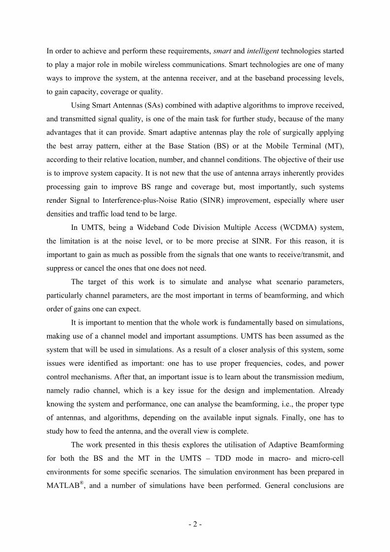
UMTS consists of three interacting domains: the User Equipment (UE) Domain,

UMTS Terrestrial Radio Access Network (UTRAN) Domain and Core Network (CN)

Domain. The high-level system architecture with network elements is shown in Figure 2.1.

Figure 2.1 – UMTS domains and network elements (extracted from [HoTo01]).

The UE Domain is responsible for access to UMTS services, which is done

via a radio interface. It consists of the UMTS Subscriber Identity Module (USIM)

and the Mobile Equipment (ME). The ME is the radio terminal used for radio communication

over the “Uu” interface. The USIM performs data and procedures for subscriber identity,

and some information that is needed at the terminal, and these functions are embedded

in a smartcard. The interface between ME and UMTS Subscriber Identity Module is

designated by the “Cu” interface.

The UTRAN Domain provides the air interface access. It is divided into Radio

Network Subsystems (RNSs). Each RNS contains the radio network element Node-B,

or Base Station (BS), and control equipment Radio Network Controller (RNC). The interface

between the Node-B and the RNC is the ‘Iub’ interface. Between RNSs there is the ‘Iur’

interface.

The CN Domain function is to provide routing, switching and data connections to

external networks. The basic CN architecture for UMTS is based on the GSM network with

- 6 -

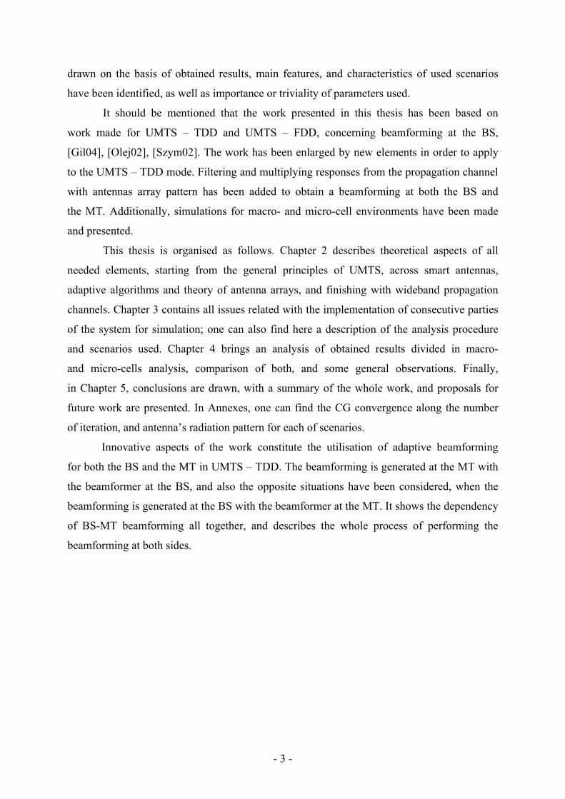
GPRS, but all elements have to be modified for UMTS operation and services. The CN

consists of the Mobile services Switching Centre (MSC), Visitor Location Register (VLR)

and Gateway MSC (GMSC). These elements are Circuit Switched (CS) domains, but the Core

Network Domain is divided in Packet Switched (PS) domains as well: Serving GPRS Support

Node (SGSN) and Gateway GPRS Support Node (GGSN). The CN also consists of the Home

Location Register (HLR), which is shared by both CS and PS domains.

The interface between the logical network elements, UE and UTRAN, is the ‘Uu’

interface, which is the WCDMA radio interface. The other interface is the ‘Iu’ located

between the UTRAN and CN.

The UMTS network architecture is shown in Figure 2.2.

UE

UE

UE

BS

BS

BS

BS

RNC

RNC

Uu UTRAN

Iur

Iu CN

Com3

latigid

Registers

HLR/AuC/EIR

3G MSC/VLR 3G GMSC

CN CS Domain

CN PS Domain

SGSN GGSN

Figure 2.2 – UMTS network architecture (extracted from [KALN01]).

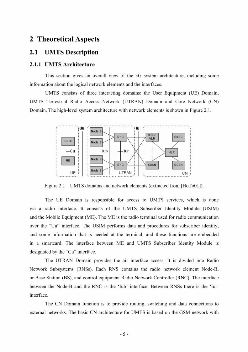
The radio interface protocol architecture around the physical layer architecture

is shown in Figure 2.3. The radio interface consists of Layers 1, 2 and 3. In UMTS there are

three types of channels related with the layer structure of the system [3GPP03a]: physical

channels, logical channels and transport channels. The physical layer interfaces the Medium

Access Control (MAC) sub-layer of Layer 2 and the Radio Resource Control (RRC) Layer

of Layer 3. The circles between different layer/sub-layers indicate Service Access Points

- 7 -

(SAPs). The physical layer offers services via transport channels to the MAC, characterised

by how the information is transferred over the radio interface.

The MAC layer offers different Logical channels to the Radio Link Control (RLC)

sub-layer of Layer 2. The logical channels are characterised by the type of information

transferred.

Physical channels are defined in the physical layer. There are two duplex modes:

Frequency Division Duplex (FDD) and Time Division Duplex (TDD). In the FDD mode

a physical channel is characterised by the code, frequency and in the UL the relative

phase (I/Q). In the TDD mode the physical channels is also characterised by the timeslot.

The physical layer is controlled by RRC.

Radio Resource Control (RRC)

Medium Access Control

Transport channels

Physical layer

Con

trol /

Mea

sure

men

ts

Layer 3

Logical channelsLayer 2

Layer 1

Figure 2.3 – Radio interface protocol architecture around the physical layer (extracted from [3GPP03a]).

2.1.2 Wideband Code Division Multiple Access

Wideband Code Division Multiple Access (WCDMA) is the radio interface, which is

implemented in UMTS. WCDMA is a wideband Direct-Sequence Code Division Multiple

Access (DS-CDMA) system, which means that user information bits are spread

over a wide bandwidth by multiplying the user data with quasi-random bits (called chips)

derived from Code Division Multiple Access (CDMA) spreading codes [HoTo01].

The new requirements of 3G systems, as described in Chapter 1, are supported. The larger

bandwidth of 5 MHz is needed to support higher bit rates. WCDMA improves the DL

capacity to support the asymmetric capacity requirements between DL and UL.

WCDMA supports two basic modes of operation: FDD and TDD. For FDD,

two separated 5 MHz radio bands for the UL and DL transmissions are required. For TDD,

a single 5 MHz band is time-shared between UL and DL. TDD is used on an unpaired band,

- 8 -

while the FDD system requires a pair of bands. FDD has one chip-rate option, the 3.84 Mcps,

whereas TDD has two options, the 3.84 Mcps and the 1.28 Mcps ones.

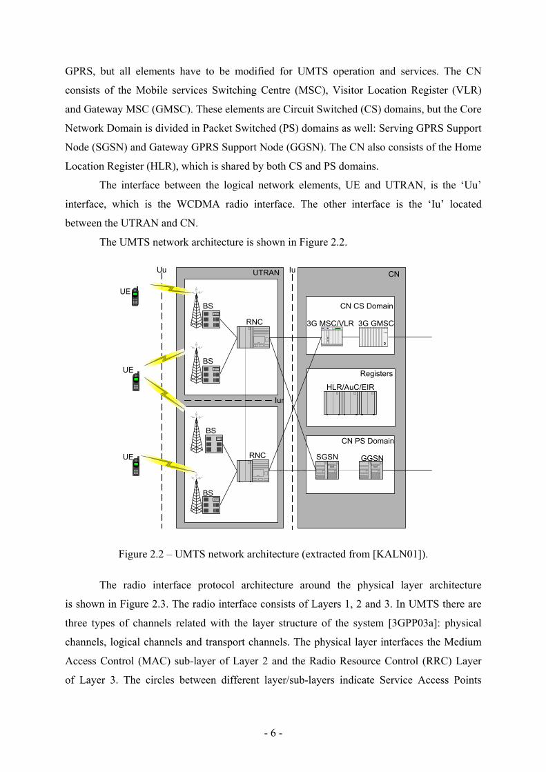
UMTS frequency bandwidth is allocated at around 2 GHz. In Europe, UMTS bands

will be available in two groups. The first one will be available for WCDMA FDD

and the second one for WCDMA TDD. The available frequency bands are:

• FDD (paired bands):

− 1920 - 1980 MHz (UL)

− 2110 - 2170 MHz (DL)

• TDD (unpaired bands):

− 1900 - 1920 MHz

− 2010 - 2025 MHz

12 radio channels are available for FDD, and 7 for TDD.

The spectrum allocation is shown in Figure 2.4.

1800 2050 21502100 2200 1950 20001850 1900

UMTS FDD

UMTS TDD

DECT MSS

GSM 1800

PHS

IS - 95 PCS

Japan

Korea

USA

Europe

f [MHz]

Figure 2.4 – Spectrum allocations in Europe, Japan, Korea, and USA (extracted from [HoTo01]).

WCDMA supports variable bit rate to offer BoD and 10 ms radio frame. In TDD, a 10 ms

radio frame is divided into 15 timeslots each of 2560 chips at the chip rate 3.84 Mcps.

Each of the 15 timeslots within a frame is allocated to either UL or DL. For the 1.28 Mcps

TDD option, a 10 ms radio frame is divided into two 5 ms sub-frame. In each sub-frame, there

are 7 normal time slots and 3 special time slots [3GPP03a].

There is no requirement for a global time reference, such as a Global Positioning

System (GPS) because WCDMA supports the operation of asynchronous BSs. WCDMA

(UL and DL)

- 9 -

employs coherent detection on UL and DL based on the use of pilot symbols or common

pilot. The use of coherent detection is new for public CDMA systems, and will result in an

overall increase of coverage and capacity on the UL.

Table 2.1 shows the main parameters of WCDMA.

Table 2.1 – Main WCDMA parameters (extracted from [HoTo01]).

Multiple access method DS-CDMA Duplexing method FDD / TDD Base station synchronization Asynchronous operation Chip rate 3.84 Mcps Frame length 10 ms Service multiplexing Multiple service with different quality of service requirements

multiplexed on one connection Multirate concept Variable spreading factor and multicode Detection Coherent using pilot symbols or common pilot Multiuser detection, smart antennas

Supported by the standard, optional in the implementation

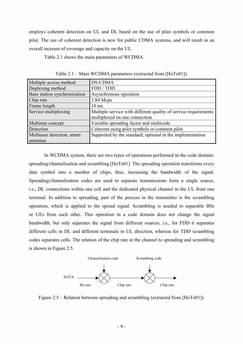
In WCDMA system, there are two types of operations performed in the code domain:

spreading/channelisation and scrambling [HoTo01]. The spreading operation transforms every

data symbol into a number of chips, thus, increasing the bandwidth of the signal.

Spreading/channelisation codes are used to separate transmissions form a single source,

i.e., DL connections within one cell and the dedicated physical channel in the UL from one

terminal. In addition to spreading, part of the process in the transmitter is the scrambling

operation, which is applied to the spread signal. Scrambling is needed to separable BSs

or UEs from each other. This operation in a code domain does not change the signal

bandwidth, but only separates the signal from different sources, i.e., for FDD it separates

different cells in DL and different terminals in UL direction, whereas for TDD scrambling

codes separates cells. The relation of the chip rate in the channel to spreading and scrambling

is shown in Figure 2.5.

DATA

Channelisation code Scrambling code

Bit rate Chip rate Chip rate

Figure 2.5 – Relation between spreading and scrambling (extracted from [HoTo01]).

- 10 -

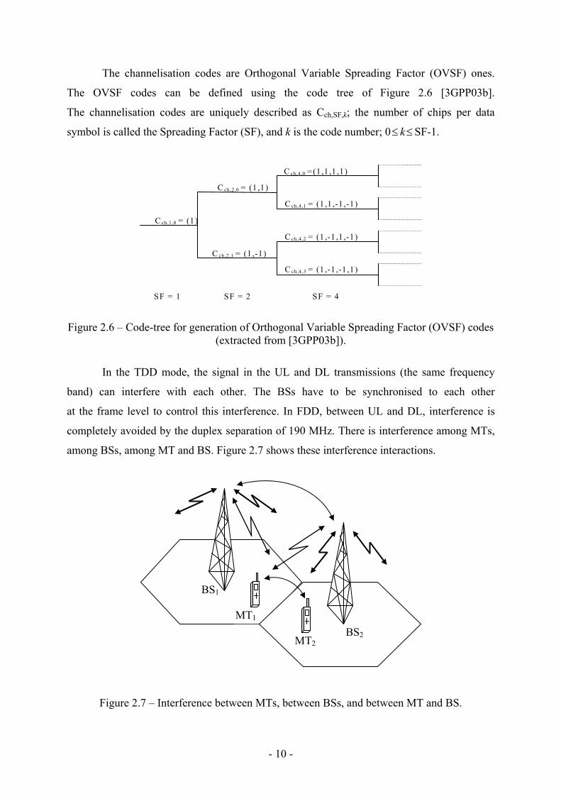
The channelisation codes are Orthogonal Variable Spreading Factor (OVSF) ones.

The OVSF codes can be defined using the code tree of Figure 2.6 [3GPP03b].

The channelisation codes are uniquely described as Cch,SF,k; the number of chips per data

symbol is called the Spreading Factor (SF), and k is the code number; 0≤ k≤SF-1.

SF = 1 SF = 2 SF = 4

C ch,1,0 = (1 )

C ch,2,0 = (1 ,1 )

C ch,2,1 = (1 ,-1)

C ch,4,0 = (1 ,1 ,1 ,1)

C ch,4,1 = (1 ,1 ,-1 ,-1)

C ch,4,2 = (1 ,-1 ,1 ,-1)

C ch,4,3 = (1 ,-1 ,-1 ,1)

Figure 2.6 – Code-tree for generation of Orthogonal Variable Spreading Factor (OVSF) codes (extracted from [3GPP03b]).

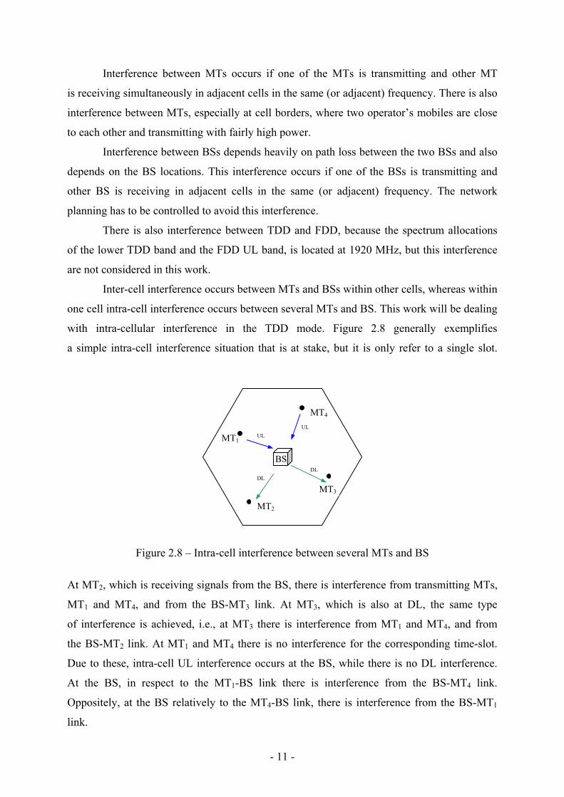
In the TDD mode, the signal in the UL and DL transmissions (the same frequency

band) can interfere with each other. The BSs have to be synchronised to each other

at the frame level to control this interference. In FDD, between UL and DL, interference is

completely avoided by the duplex separation of 190 MHz. There is interference among MTs,

among BSs, among MT and BS. Figure 2.7 shows these interference interactions.

Figure 2.7 – Interference between MTs, between BSs, and between MT and BS.

MT1

BS1

MT2BS2

- 11 -

Interference between MTs occurs if one of the MTs is transmitting and other MT

is receiving simultaneously in adjacent cells in the same (or adjacent) frequency. There is also

interference between MTs, especially at cell borders, where two operator’s mobiles are close

to each other and transmitting with fairly high power.

Interference between BSs depends heavily on path loss between the two BSs and also

depends on the BS locations. This interference occurs if one of the BSs is transmitting and

other BS is receiving in adjacent cells in the same (or adjacent) frequency. The network

planning has to be controlled to avoid this interference.

There is also interference between TDD and FDD, because the spectrum allocations

of the lower TDD band and the FDD UL band, is located at 1920 MHz, but this interference

are not considered in this work.

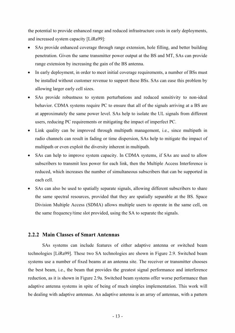
Inter-cell interference occurs between MTs and BSs within other cells, whereas within

one cell intra-cell interference occurs between several MTs and BS. This work will be dealing

with intra-cellular interference in the TDD mode. Figure 2.8 generally exemplifies

a simple intra-cell interference situation that is at stake, but it is only refer to a single slot.

Figure 2.8 – Intra-cell interference between several MTs and BS

At MT2, which is receiving signals from the BS, there is interference from transmitting MTs,

MT1 and MT4, and from the BS-MT3 link. At MT3, which is also at DL, the same type

of interference is achieved, i.e., at MT3 there is interference from MT1 and MT4, and from

the BS-MT2 link. At MT1 and MT4 there is no interference for the corresponding time-slot.

Due to these, intra-cell UL interference occurs at the BS, while there is no DL interference.

At the BS, in respect to the MT1-BS link there is interference from the BS-MT4 link.

Oppositely, at the BS relatively to the MT4-BS link, there is interference from the BS-MT1

link.

MT2

MT1

MT3

MT4

BS

DL DL

UL UL

- 12 -

Besides the interference issue, Power Control (PC) is an important aspect in WCDMA

and is needed to keep the interference levels at minimum in the radio interface and also

to supply the required Quality of Service (QoS). In the DL, PC is used to minimise

the interference to other cells and compensating for other cells interference. In the UL,

an important problem that PC avoids is the near-far effect. In near-far situations, the signal of

the MT that is close to the serving BS may dominate over the signal of the MTs that are far

away from the same BS. PC avoids this problem, by making the transmission power level

received from all terminals as equal and low as possible at the home cell, for the same QoS

[Szym02].

In UMTS, PC has two types of loops, Open Loop Power Control (OLPC) and Closed

Loop Power Control (CLPC). OLPC is used to adjust the output power of the received signal

level from the BS to a specific value. It is used for setting initial transmission powers when

the MT is connecting to the network. CLPC consists of two different loops: Outer Loop

Power Control and Inner Loop Power Control. Inner Loop Power Control is the fastest loop in

WCDMA power control mechanism, which is called Fast Closed Loop Power Control. Outer

loop power control is used to maintain the required QoS, while using as low power as

possible, whereas Inner Loop Power Control is used to keep the received Signal-to-

Interference Ratio (SIR) at a given target and also to command the MT to increase or decrease

its transmission power, with a cycle of 1.5 kHz, by 1, 2 or 3 dB step-sizes [HoTo01].

2.2 Smart Antennas and Adaptive Algorithms

2.2.1 Key Features of Smart Antennas

This section presents key features of smart antennas, including switched beam system

and adaptive antenna concepts, especially focusing on adaptive beamforming algorithms.

Smart Antennas (SAs) are a new technology for the application in wireless systems.

These, most often, use a fixed set of antenna elements in an array, and offer a broad range of

ways to improve wireless system performance. The signal from these antenna elements are

combined to form a movable beam pattern that can be steered. Most simplistically, a beam

may be pointed to the desired direction that tracks mobile units as they move, using either

digital signal processing, or Radio Frequency (RF) hardware. SA systems contribute to

minimising the impact of noise and interference for each MT and BS. In general, SAs have

- 13 -

the potential to provide enhanced range and reduced infrastructure costs in early deployments,

and increased system capacity [LiRa99]:

• SAs provide enhanced coverage through range extension, hole filling, and better building

penetration. Given the same transmitter power output at the BS and MT, SAs can provide

range extension by increasing the gain of the BS antenna.

• In early deployment, in order to meet initial coverage requirements, a number of BSs must

be installed without customer revenue to support these BSs. SAs can ease this problem by

allowing larger early cell sizes.

• SAs provide robustness to system perturbations and reduced sensitivity to non-ideal

behavior. CDMA systems require PC to ensure that all of the signals arriving at a BS are

at approximately the same power level. SAs help to isolate the UL signals from different

users, reducing PC requirements or mitigating the impact of imperfect PC.

• Link quality can be improved through multipath management, i.e., since multipath in

radio channels can result in fading or time dispersion, SAs help to mitigate the impact of

multipath or even exploit the diversity inherent in multipath.

• SAs can help to improve system capacity. In CDMA systems, if SAs are used to allow

subscribers to transmit less power for each link, then the Multiple Access Interference is

reduced, which increases the number of simultaneous subscribers that can be supported in

each cell.

• SAs can also be used to spatially separate signals, allowing different subscribers to share

the same spectral resources, provided that they are spatially separable at the BS. Space

Division Multiple Access (SDMA) allows multiple users to operate in the same cell, on

the same frequency/time slot provided, using the SA to separate the signals.

2.2.2 Main Classes of Smart Antennas

SAs systems can include features of either adaptive antenna or switched beam

technologies [LiRa99]. These two SA technologies are shown in Figure 2.9. Switched beam

systems use a number of fixed beams at an antenna site. The receiver or transmitter chooses

the best beam, i.e., the beam that provides the greatest signal performance and interference

reduction, as it is shown in Figure 2.9a. Switched beam systems offer worse performance than

adaptive antenna systems in spite of being of much simples implementation. This work will

be dealing with adaptive antennas. An adaptive antenna is an array of antennas, with a pattern

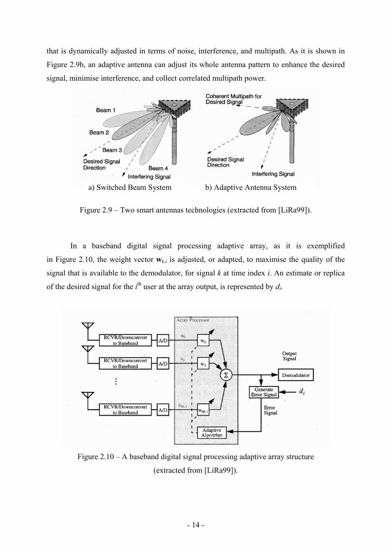
- 14 -

that is dynamically adjusted in terms of noise, interference, and multipath. As it is shown in

Figure 2.9b, an adaptive antenna can adjust its whole antenna pattern to enhance the desired

signal, minimise interference, and collect correlated multipath power.

a) Switched Beam System b) Adaptive Antenna System

Figure 2.9 – Two smart antennas technologies (extracted from [LiRa99]).

In a baseband digital signal processing adaptive array, as it is exemplified

in Figure 2.10, the weight vector wk,i is adjusted, or adapted, to maximise the quality of the

signal that is available to the demodulator, for signal k at time index i. An estimate or replica

of the desired signal for the ith user at the array output, is represented by di.

Figure 2.10 – A baseband digital signal processing adaptive array structure

(extracted from [LiRa99]).

- 15 -

2.2.3 Main Adaptive Beamforming Algorithms

A generic non-blind adaptive beamforming system is shown in Figure 2.11.

The selection of the weight vector w is based on the signal vector x(t) received at the array

and reference signal if such signal is required, d*(t). The objective of beamforming

is to optimise the beamformer response with respect to a prescribed criterion, so that

the output y(t) contains minimal contribution from noise and interference.

Figure 2.11 – A generic adaptive beamforming system (extracted from [LiLo96]).

There are a number of criteria for choosing the optimum weights [LiLo96]:

• Minimum Mean-Square Error (MMSE) attempts to minimise the difference between

the array output and some desired signal.

• Maximum Signal-to-Noise Ratio (Max SNR) maximises the actual signal-to-noise

ratio at the array output.

• Linear Constrained Minimum Variance (LCMV) minimises the variance at the output

of the array.

• Multiple Sidelobe Canceller (MSCl), which goal is to choose the auxiliary channel

weights to cancel the main channel interference component.

The selection of a criterion is not critically important in terms of performance,

but it is important in terms of what information about the incoming signal is available

[Szym02]. Depending on how the weights are chosen, the beamforming is divided between

data independent or statistically optimum [VeBu88]. In a data independent, the weights do not

depend on the array data and are chosen to present a specified response for all

signal/interference scenarios. In a statistically optimum beamforming the weights are chosen

based on the statistics of the data received at the array, to “optimise” the array response, i.e.,

the beamformer output contains minimal contributions due to noise and signal arriving from

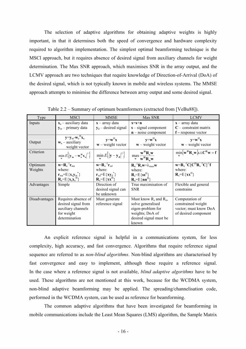
different directions than the desired signal. Table 2.2 summarises their main characteristics.

- 16 -

The selection of adaptive algorithms for obtaining adaptive weights is highly

important, in that it determines both the speed of convergence and hardware complexity

required to algorithm implementation. The simplest optimal beamforming technique is the

MSCl approach, but it requires absence of desired signal from auxiliary channels for weight

determination. The Max SNR approach, which maximises SNR in the array output, and the

LCMV approach are two techniques that require knowledge of Direction-of-Arrival (DoA) of

the desired signal, which is not typically known in mobile and wireless systems. The MMSE

approach attempts to minimise the difference between array output and some desired signal.

Table 2.2 – Summary of optimum beamformers (extracted from [VeBu88]). Type MSCl MMSE Max SNR LCMV

Inputs xa – auxiliary data ym – primary data

x – array data yd – desired signal

x=s+n s – signal component n – noise component

x – array data C – constraint matrix f – response vector

Output y=ym-wa

Hxa wa – auxiliary

weight vector

y=wHx w – weight vector



Criterion { }2min a

Hamw

xwy −E { }2min dwyy −E

wRwwRw

nH

sH

wmax { } fwCwRw H

xH

w=s.t.min

Optimum Weights

w=Ra-1rma

where: rma=E{xaym

*} Ra=E{xaxa

H}

w=Rx-1rxd

where: rxd=E{xyd

*} Rx=E{xxH}

Rn-1Rsw=λmaxw

where: Rs=E{ssH} Rn=E{nnH}

w=Rx-1C[CHRx

-1C]-1f where: Rx=E{xxH}

Advantages Simple Direction of desired signal can be unknown

True maximisation of SNR

Flexible and general constrains

Disadvantages Requires absence of desired signal from auxiliary channels for weight determination

Must generate reference signal

Must know Rs and Rn, solve generalised eigen-problem for weights; DoA of desired signal must be known

Computation of constrained weight vector; must know DoA of desired component

An explicit reference signal is helpful in a communications system, for less

complexity, high accuracy, and fast convergence. Algorithms that require reference signal

sequence are referred to as non-blind algorithms. Non-blind algorithms are characterised by

fast convergence and easy to implement, although these require a reference signal.

In the case where a reference signal is not available, blind adaptive algorithms have to be

used. These algorithms are not mentioned at this work, because for the WCDMA system,

non-blind adaptive beamforming may be applied. The spreading/channelisation code,

performed in the WCDMA system, can be used as reference for beamforming.

The common adaptive algorithms that have been investigated for beamforming in

mobile communications include the Least Mean Squares (LMS) algorithm, the Sample Matrix

- 17 -

Inversion (SMI) technique and Recursive Least Squares (RLS) algorithm [LiLo96].

The simplest algorithm to implement is the LMS one, but it has its drawbacks: the dynamic

range over which it operates is quite limited. If dynamic range increases more than

the permissible order, PC is required if the LMS algorithm is to be used. The SMI approach

offers a relatively fast convergence rate, but in order to achieve it, the direct inversion of the

covariance matrix should be employed. If we know a priori the desired and interference

signal, then the covariance matrix could be evaluated and the optimal solution for the weights

could be computed using SMI [LiLo96]. An important feature of the RLS Algorithm

[LiLo96], [GiMC01] is that the inversion of covariance matrix is replaced at each step by a

simple scalar division, and it reduces the computational complexity while maintaining a

similar performance. The RLS approach offers an order of magnitude faster convergence rate

than the LMS algorithm, provided that the signal-to-noise ratio is high.

There are other adaptive techniques, which have also been applied to beamforming in

mobile communications. These techniques include the Conjugate Gradient (CG) method, the

Linear Least Squares Error (LLSE) algorithm, the method based on rotational invariance, and

the Hopfield neural network [LiLo96]. All these methods have been proposed to either

improve the performance or level the shortcomings of the LMS, SMI, or RLS algorithms.

The mentioned algorithms, generally described in this subsection, are just examples

of different approaches to the beamforming problem, because the variety of approaches

is very rich. In the next section, the CG algorithm is described in more detail.

As results of dealing with adaptive beamforming algorithms, the objective is to

calculate the Beamforming Gain (BG), and Signal to Interference-plus-Noise Ratio (SINR)

for a single antenna’s element and for each link.

The calculation of SINR for the lth link follows, [Gil04]:

∑=

+

⋅=

T

T

L

l

lNDesI

pl

DesSl

NP

GPSINR

1

)(

)()( , (2.1)

where:

• Gp – CDMA processing gain (equal to the spreading factor);

• PDesS – Desired Signal (DesS) power;

• PNDesI –Non-Desired Interference (NDesI) power;

• N – total noise power.

- 18 -

The lth BG at the BS, Gbeamformer (BS), is defined as the SINR gain relative to the SINR achieved

with a single omnidirectional antenna at the BS, for each of the L active links:

( ) ( ) BS singlebeamformerBSbeamformer)l()l()l( SINRSINRG −= [dB], (2.2)

whereas, the lth BG at the MT, Gbeamformer (MT), is defined as the SINR gain relative to the SINR

achieved with a single omnidirectional antenna at the MT, for each of the L active links:

( ) ( )MT singlebeamformerMTbeamformer)l()l()l( SINRSINRG −= [dB]. (2.3)

2.2.4 Conjugate Gradient Algorithm

The Conjugate Gradient (CG) can be applied to adjust the weights of an antenna array

[GiMC01]. The CG algorithm has been well defined and described in the recent years as an

alternative to the widely used LMS and RLS. With the argument of not requiring matrix

inversions and avoiding stability problems, the Conjugate Directions type of algorithms, such

as the CG, have been conceived for solving linear systems, [HeBK99], [Goda97].

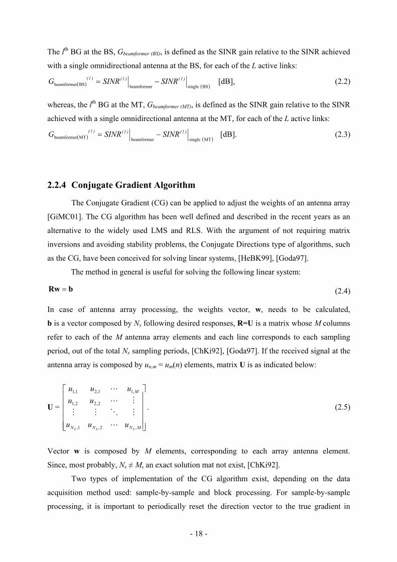
The method in general is useful for solving the following linear system:

=Rw b (2.4)

In case of antenna array processing, the weights vector, w, needs to be calculated,

b is a vector composed by Ns following desired responses, R=U is a matrix whose M columns

refer to each of the M antenna array elements and each line corresponds to each sampling

period, out of the total Ns sampling periods, [ChKi92], [Goda97]. If the received signal at the

antenna array is composed by un,m = um(n) elements, matrix U is as indicated below:

U =

MNNN

M

SSSuuu

uuuuu

,2,1,

2,22,1

,11,21,1

. (2.5)

Vector w is composed by M elements, corresponding to each array antenna element.

Since, most probably, Ns ≠ M, an exact solution mat not exist, [ChKi92].

Two types of implementation of the CG algorithm exist, depending on the data

acquisition method used: sample-by-sample and block processing. For sample-by-sample

processing, it is important to periodically reset the direction vector to the true gradient in

- 19 -

order to ensure the convergence of the algorithm. Besides sample-by-sample processing,

the block-by-block method also exists. Block-by-block CG implementation requires that both

R and b be firstly calculated. The computational complexity of this implementation depends

on K (K≤N), the number of iterations. For large N the computational complexity of the

algorithm is K times of the complexity of the sample-by-sample CG algorithm [Bagh99].

2.3 Antenna Arrays

Usually, the radiation pattern of a single element is relatively wide, higher gains only

being achieved by increasing the electric size of the antenna. In many type of communication,

antennas with very high directivity are often required. Another way to increase the electrical

size of an antenna is to construct it as an assembly of radiating elements in a proper electrical

and geometrical configuration antenna array. Usually the array elements are identical; this is

not necessary, but it is more practical, simple and convenient for design and fabrication,

and the individual elements may be of any type (wire dipoles or loops, apertures, etc.).

That constitutes a Uniform Array. The radiating characteristics of an array can be electrically

controlled by the amplitude and relative phase of each individual element’s feeding current,

providing means for the deployment of adaptive antennas algorithms.

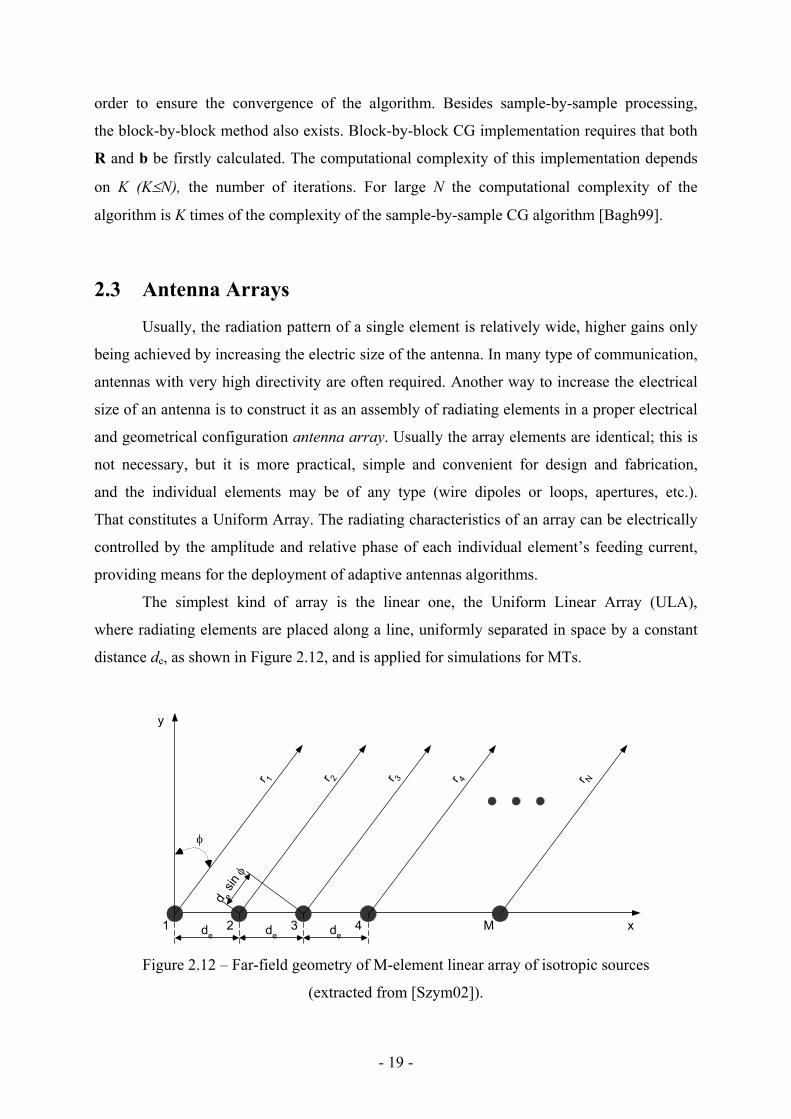
The simplest kind of array is the linear one, the Uniform Linear Array (ULA),

where radiating elements are placed along a line, uniformly separated in space by a constant

distance de, as shown in Figure 2.12, and is applied for simulations for MTs.

φ

1 2 3 4deM

d e si

n φ

x

y

r 1 r 4r 3r 2 r N

de de Figure 2.12 – Far-field geometry of M-element linear array of isotropic sources

(extracted from [Szym02]).

- 20 -

An array of identical elements, all of identical magnitude, and each with a progressive phase,

is referred to as a uniform array. The Array Factor (AF) of an M-element ULA of isotropic

sources is given by:

( )∑=

ψ−=M

n

nje1

1AF (2.6)

where γ+φ=ψ sinkd , or yet as a closed form, which is more convenient for pattern analysis

ψ

ψ

⋅=ψ

−

2

2AF 21

sin

Msine

Mj (2.7)

The maximum value of the magnitude of the AF is equal to M. To normalise the array factor

so that the maximum value is equal to unity, the AF is written in normalised form as

ψ

ψ

=

2

21AFsin

Msin

Mn (2.8)

In the case of adaptive beamforming, ULA elements can be fed with different magnitudes

and phases respectively to the weights vector provided by adaptive processor. If the elements

are of any other than isotropic pattern, the total field pattern can be obtained by simply

multiplying the AF by the normalised field pattern of the individual element [Bala97].

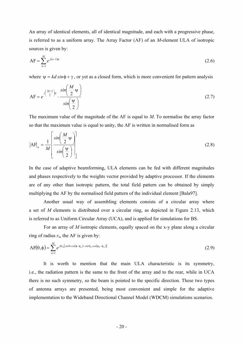
Another usual way of assembling elements consists of a circular array where

a set of M elements is distributed over a circular ring, as depicted in Figure 2.13, which

is referred to as Uniform Circular Array (UCA), and is applied for simulations for BS.

For an array of M isotropic elements, equally spaced on the x-y plane along a circular

ring of radius ra, the AF is given by:

( ) ( ) ( )[ ]∑=

φ−φθ−φ−φθ=φθM

n

cossincossinjkr nnae1

00,AF (2.9)

It is worth to mention that the main ULA characteristic is its symmetry,

i.e., the radiation pattern is the same to the front of the array and to the rear, while in UCA

there is no such symmetry, so the beam is pointed to the specific direction. These two types

of antenna arrays are presented, being most convenient and simple for the adaptive

implementation to the Wideband Directional Channel Model (WDCM) simulations scenarios.

- 21 -

φ

θ

φn

ra

M 1 2

x

y

z

r

Rn

n

Figure 2.13 – Geometry of an M-element circular array (extracted from [Szym02]).

2.4 Wideband Propagation Channels

2.4.1 Introduction

The structure of the radio channel should be known in order to deal with beamforming

and SAs. At the present, with the introduction of techniques and features that depend on

the spatial distribution of the mobiles, wideband temporal and spatial information is required

for relevant channel models.

Depending on the numbers of parameters used to build various channel models, one

can divide them into: non-directional and directional ones. Classical, non-directional, channel

models provide information on signal power level distributions and Doppler shifts of the

received signal. Fundamental principles of the classical channel models are used to describe

other spatial models. Early channel models accounted only for the time-varying amplitude and

phase of channel. Recent, directional, channel models include both spatial and temporal

features for design of wideband models; these spatial channel models build upon the classical

understanding of multipath fading and Doppler spread, by incorporating additional concepts

such as time delay spread, Angle-Of-Arrival (AoA), and adaptive array antenna geometries

[LiRa99].

In a wireless system, a signal transmitted through the channel interacts with the

environment in a very complex way. There are reflections from large objects, diffraction of

- 22 -

the electromagnetic waves around objects, and signal scattering. The result of these complex

interactions is the presence of many signal components, or multipath signals, at the receiver.

Several directional channel models are described in detail in [LiRa99].

In the subsequent part of this section only WDCMs, based on Geometrically Based Single

Bounce (GBSB) Models, are introduced.

2.4.2 Geometrically Based Single Bounce Models

Geometrically Based Single Bounce (GBSB) Statistical Channel Models

are developed by defining a spatial scatterer density function [LiRa99]. From the spatial

scatterer density function, it is possible to derive the joint and marginal Time-of-Arrival

(ToA) and Direction-of-Arrival (DoA) probability density functions (PDF). Knowledge of

these statistics is useful for evaluating adaptive antenna performance. The PDF delimiting

region is discussed in what follows, leading to two different models, which are based on a

scatterer region of circular and elliptical shapes, the GBSB Circular Model (GBSBCM)

and GBSB Elliptical Model (GBSBEM).

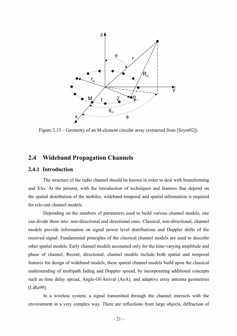
The GBSBCM is applicable to macro-cell environments. In a macro-cell environment,

the BS is typically deployed above the surrounding scatterers, i.e., antenna heights are

relatively high, therefore assuming that there will be no signal scattering from locations near

the BS. Figure 2.14 shows a circular scatterer region of radius rmax surrounding the MT.

φ0

dT

rmaxMT

BS

Figure 2.14 – Geometry for the GBSBCM scattering region (extracted from [ZoMa00]).

- 23 -

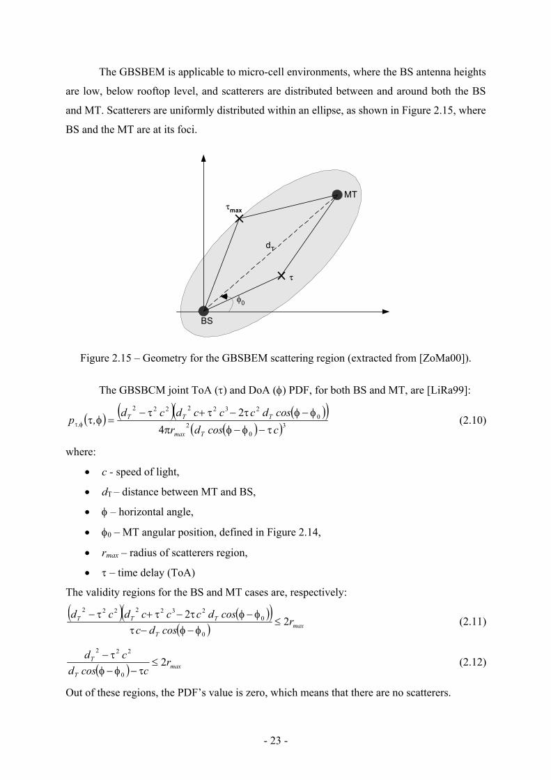
The GBSBEM is applicable to micro-cell environments, where the BS antenna heights

are low, below rooftop level, and scatterers are distributed between and around both the BS

and MT. Scatterers are uniformly distributed within an ellipse, as shown in Figure 2.15, where

BS and the MT are at its foci.

φ0

BS

MT

τ

τmax

dT

Figure 2.15 – Geometry for the GBSBEM scattering region (extracted from [ZoMa00]).

The GBSBCM joint ToA (τ) and DoA (φ) PDF, for both BS and MT, are [LiRa99]:

( ) ( ) ( )( )( )( )30

20

2322222

42

ccosdrcosdcccdcd

,pTmax

TTT,

τ−φ−φπ

φ−φτ−τ+τ−=φτφτ (2.10)

where:

• c - speed of light,

• dT – distance between MT and BS,

• φ – horizontal angle,

• φ0 – MT angular position, defined in Figure 2.14,

• rmax – radius of scatterers region,

• τ – time delay (ToA)

The validity regions for the BS and MT cases are, respectively:

( ) ( )( )( ) max

T

TTT rcosdc

cosdcccdcd2

2

0

02322222

≤φ−φ−τ

φ−φτ−τ+τ− (2.11)

( ) maxT

T rccosd

cd2

0

222

≤τ−φ−φ

τ− (2.12)

Out of these regions, the PDF’s value is zero, which means that there are no scatterers.

- 24 -

For the GBSBEM, the joint PDF observed at the BS (or MT) is given by [LiRa99]:

( )( ) ( )( )

( )( )

τ≤τ≤

τ−φ−φ−τπτ

φ−φτ−τ+τ−

=φτφτ

elsewhere, 0

,2

30

222

02322222

maxT

TTmaxmax

TTT

, cd

ccosddcc

cosdcccdcd,p (2.13)

Note that the above PDF is independent of the scattering/clustering density, for it

assumes a continuous scattering distribution. However, in a simulation case, cluster density

should be a parameter to take into account [ZoMa00].

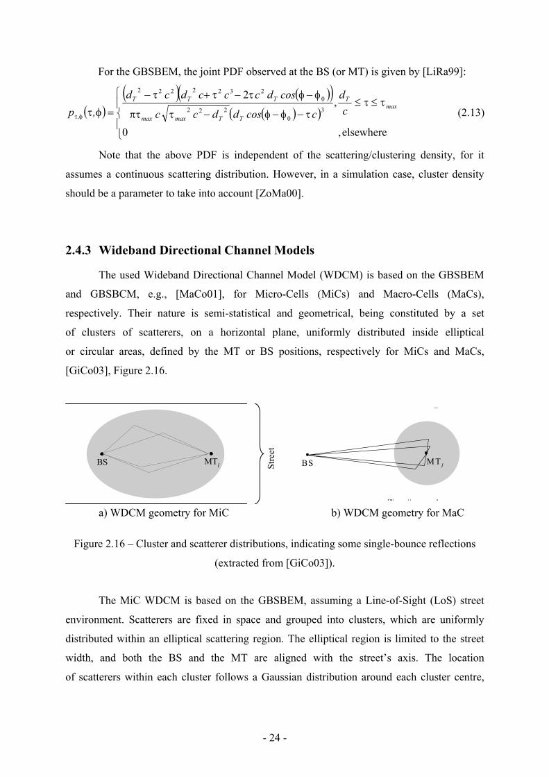
2.4.3 Wideband Directional Channel Models

The used Wideband Directional Channel Model (WDCM) is based on the GBSBEM

and GBSBCM, e.g., [MaCo01], for Micro-Cells (MiCs) and Macro-Cells (MaCs),

respectively. Their nature is semi-statistical and geometrical, being constituted by a set

of clusters of scatterers, on a horizontal plane, uniformly distributed inside elliptical

or circular areas, defined by the MT or BS positions, respectively for MiCs and MaCs,

[GiCo03], Figure 2.16.

MTlBS

BS MT l

a) WDCM geometry for MiC b) WDCM geometry for MaC

Figure 2.16 – Cluster and scatterer distributions, indicating some single-bounce reflections

(extracted from [GiCo03]).

The MiC WDCM is based on the GBSBEM, assuming a Line-of-Sight (LoS) street

environment. Scatterers are fixed in space and grouped into clusters, which are uniformly

distributed within an elliptical scattering region. The elliptical region is limited to the street

width, and both the BS and the MT are aligned with the street’s axis. The location

of scatterers within each cluster follows a Gaussian distribution around each cluster centre,

Stre

et

- 25 -

Figure 2.16a. Scattering coefficients are random variables, assumed uniformly distributed

in amplitude and phase within [0, 1] and [0, 2π[, respectively.

Besides the scenario perspective for MiC, the MaC WDCM, based on the GBSBCM,

also follows the same philosophy, Figure 2.16b. The main difference is that the scattering

region is a circular one, being centred at the MT. Also, the MaC model is not applicable to

the street width.

That two presented models for MiC and MaC are chosen for simulations, because

of their simplicity. They are based on the GBSB models, adding the characteristic feature

of being statistical to better approximate the enormous variety of channel conditions.

The Modified GBSB (MGBSB) Models were created for simulation purposes

[Marq01], taking into consideration the temporal evolution of the channel due to motion.

It should be mentioned that the MGBSB Models used for this work, derived on IST-FLOWS

(Flexible Convergence of Wireless Standard and Services) proposals [DGVC03].

The number of clusters per model usually is not more than 10 and, for simulation, 7 clusters

per model are enough.

- 26 -

- 27 -

3 Implementation

3.1 General Concept of Performing the Simulation

This chapter is concentrated in the description of the models and algorithms

implemented for macro- and micro-cell scenarios. The chosen scenarios introduce one MT

and one BS. For that, the main parameters of the channel and general concept of performing

the simulations will be firstly described.

The problem presented in this work deals with the implementation of beamforming

at both the BS and the MT in the UMTS - TDD mode, and its analysis, regarding the physical

wideband and directional characteristics of the channel. The analysis will be based on creating

and comparing the chosen scenarios. A beamforming algorithm will control the adaptive

arrays at both the BS and the MT ends, in order to minimise co-channel interference, within

the same cell.

At first, the main input and output parameters of the channel should be defined.

For the channel models simulation, environment type (MiC or MaC), the MT-BS distance,

MT and BS antenna array parameters and scattering region also need to be defined. The other

parameters concerning scatterer and cluster specific properties are listed below, [Szym02]:

• region limitation (τmax or rmax)

• cluster distribution – uniform within the scattering region

• cluster characteristics

o distribution of scatterers within the clusters – Gaussian

o cluster density

o number of scatterers in each cluster – determined by a Poisson distribution

o average number of scatterers in each cluster

• scatterer characteristics

o scattering coefficient amplitude distribution – uniform, within [0,1]

o scattering coefficient phase distribution – uniform, within [0,2π[

• path attenuation coefficient

• presence or absence of LoS in the MaC case

All of these parameters are used for channel simulation, having been previously defined

according to two model assessments in IST-ASILUM (Advanced Signal Processing Schemes

for Link Capacity Increase in UMTS), [Hera00] and IST-FLOWS, [DGVC03]. For simulation

purposes, the parameters of the channel have been chosen according to IST-FLOWS,

- 28 -

[DGVC03]. Some of these parameters are scenario specific, and some are scenario

independent and common for all. Clusters distribution is uniform within the scattering region,

and cluster density has been set to 5*10-5 m-2. The distribution of scatterers within clusters is

Gaussian, with average number of scatterers per cluster of 20. Relative delays are considered

as integer multiples of the chip duration, 0.26 µs, for a chip rate of 3.84 Mchip/s, and all

incoming signals are assumed to arrive at the same instant of time, only allowing for inter-

cluster delays, [GiCo02].

For simulation, the IST/TUL Wideband Double Directional Channel Model

(IST/TUL – WDDCM) simulation software will be applied. The simulation software

generates the magnitudes (or power), delay (or ToA), phase, AoA and AoD of each scattered

ray as outputs from a simulation concretisation, or from a programmed sequence

of concretisations. The output parameters of the channel, obtained from the WDDCM

and referred to the Directional Channel Impulse Responses (DCIRs) are the main input

parameter for the present implementation. A DCIR provides the information on AoA, AoD,

ToA, magnitude (or power) and phase of incoming signal, which are required from

the wideband system perspective and also to take into account the directional requirements

of beamforming. The angular resolution of WDDCM used in simulations has been set to 0.5°,

[Gil04].

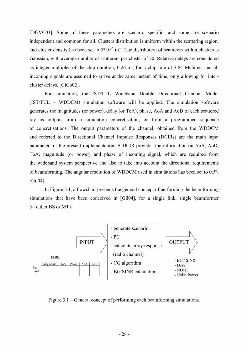
In Figure 3.1, a flowchart presents the general concept of performing the beamforming

simulations that have been conceived in [Gil04], for a single link, single beamformer

(at either BS or MT).

Figure 3.1 – General concept of performing each beamforming simulations.

INPUT

DCIRs:

Magnitude ToA Phase AoA AoD Ray1 Ray2 ....

- BG / SINR - DesS - NDesI - Noise Power

OUTPUT

- generate scenario

- PC

- calculate array response

(radio channel)

- CG algorithm

- BG/SINR calculation

- 29 -

The simulator gives a regular text file with 5 columns, for each DCIR, and each of the

columns corresponds to different parameters associated to each ray. The first column, in this

file, is magnitude, then ToA, phase, AoA, and AoD respectively.

It should be mentioned that the general block of Figure 3.1, considers:

• Generation of chosen scenarios

• Implementation of PC

• Calculation of array response (radio channel)

• Implementation of CG algorithm

• BG / SINR calculation.

Generation of chosen scenarios will be followed with the description given by separate parts,

Section 3.2, whereas the rest of these several elements of the simulation flowchart will be

described below.

A PC mechanism has been applied, using MATLAB® (file power_control.m).

A simple but effective PC process is implemented, in order to avoid near-far effects.

The PC algorithm, which has been applied for simulations, is described in [Gil04].

The next step to perform the beamforming simulations, the calculation of array

responses, depends on the number of L active BS-MT links and the number of antenna

elements, M. For each array element, for all active BS-MT links and for each time and angle

sample of the DCIR, each element of array responses is a product of:

• combination of channelisation and scrambling codes, which characterises each active

BS-MT pair

• DCIR magnitude

• DCIR phase

• antenna Array Factor (amplitude + phase)

As a result of this multiplication, channel matrices are obtained for all L active links.

These results are added with antenna thermal noise, N, creating a single array response

matrix [Gil04].

Making use of previous work, [Szym02], the CG algorithm has been applied as an

internal function (pcg.m), to control the beamforming process, by choosing the weights

vector. This is consistent with the description provided in Section 2.2.4.

As it is shown in Figure 3.1, as an output, the objective is to calculate the BG

and SINR for a single antenna’s element and for each link, as it was described

in Section 2.2.3. For all simulations, only SINR and BG values from the number of iteration

- 30 -

obtained for maximum SINR will be taken into account. The average value of SINR and BG

is obtained from 300 concretisations, as well as the standard deviation, giving a view on the

whole distribution of values, and to ensure that the number of concretisation is sufficient.

Besides evaluating SINR and BG, it is important to mention other outputs, which could be

analysed, the Desired Signal (DesS), Non-Desired Interference (NDesI) and noise power

components.

To obtain the reference source for the non-blind adaptive algorithm implementation,

TDD channelisation and scrambling code sequences combination are generated. The codes

have been applied, using MATLAB ®, and built according to the code tree, as it is shown

in Figure 2.6. The code length is constant and equal to 16, and SF is set to 4.

Simulations are performed using linear and circular arrays with different number

of elements, 8 for ULA, with element spacing of λ/2, oriented with its normal in the direction

considered as 0°, which is coincident with the LoS direction, on the same horizontal plane

as the WDCM, and 12 for UCA with element spacing of 3/4 λ. The 180° sectorisation

has been considered for ULA case, assuming also that antenna array has a ground backplane,

ideally not receiving any signals from behind. This concept has been chosen according to

[Szym02].

The general structure and some components of the simulations, for this work,

have been derived on the basis of work made for UMTS - FDD mode, with an adaptive array

at the BS, [Szym02], [Olej02], with the following changes for the UMTS - TDD mode

application:

• scrambling sequences and channelisation codes for TDD mode have been added

to substitute the FDD codes,

• filtering of DCIRs needs to be apply to get the ToA per each chip duration,

and AoD that are need in case of dealing with the beamforming at the both side,

• moreover, the whole structure of the program has been changed to obtain as main

target, beamforming at both the BS and the MT.

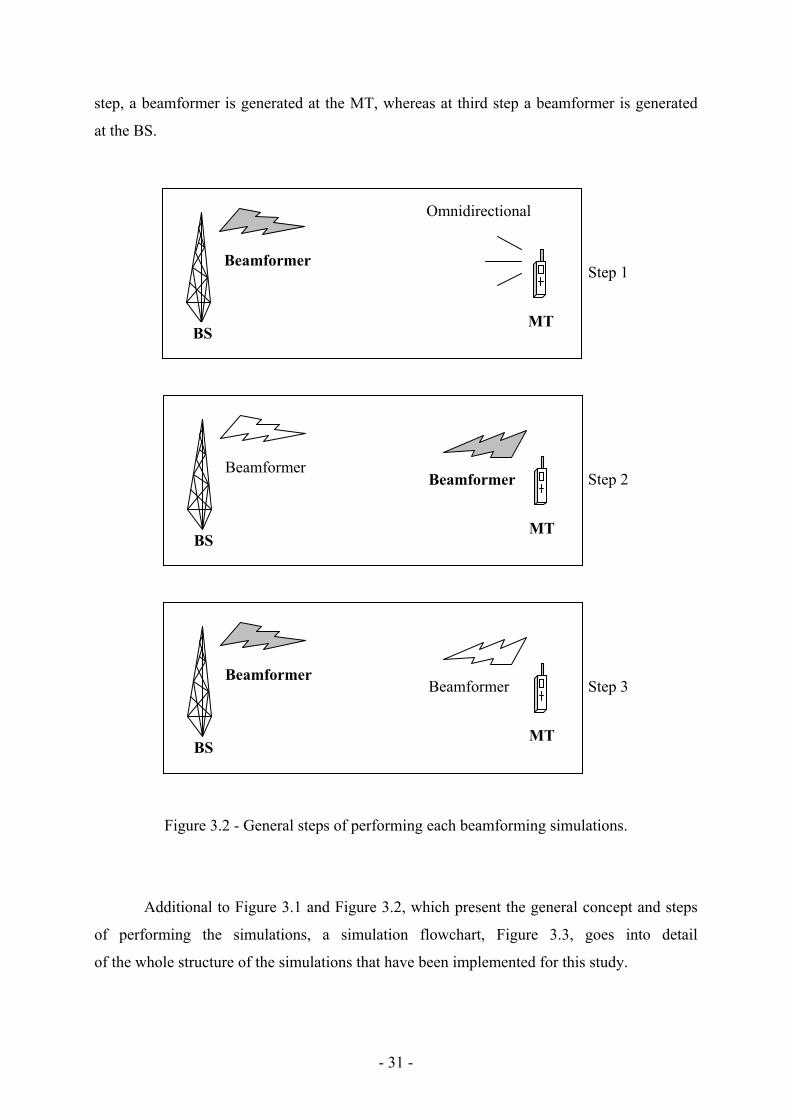
The general steps of performing each beamforming simulations, to obtain

beamforming at both the BS and the MT, are shown in Figure 3.2. The first step depicts

a beamforming only at the BS, i.e., the MT transmitting to the BS with a single,

omnidirectional antenna and beamformer is generated at the BS. The two other steps depict

the main concept of this study, beamforming at the both the BS and the MT. At the second

- 31 -

step, a beamformer is generated at the MT, whereas at third step a beamformer is generated

at the BS.

Figure 3.2 - General steps of performing each beamforming simulations.

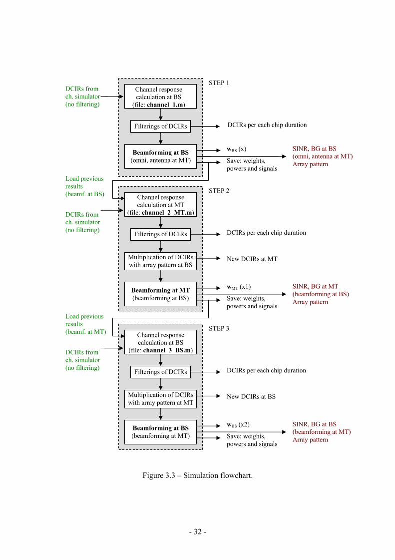
Additional to Figure 3.1 and Figure 3.2, which present the general concept and steps

of performing the simulations, a simulation flowchart, Figure 3.3, goes into detail

of the whole structure of the simulations that have been implemented for this study.

BS MT

Beamformer

BS MT

Beamformer Beamformer

Step 1

Step 2

Step 3

BS MT

Beamformer Beamformer

Omnidirectional

- 32 -

Figure 3.3 – Simulation flowchart.

STEP 1

Filterings of DCIRs

Channel response calculation at BS

(file: channel 3 BS.m)

DCIRs from ch. simulator (no filtering)

wBS (x)

Save: weights, powers and signals

SINR, BG at BS (omni, antenna at MT) Array pattern


Load previous results (beamf. at BS)

SINR, BG at MT (beamforming at BS) Array pattern Save: weights,

powers and signals Load previous results (beamf. at MT)


Beamforming at BS (beamforming at MT)

New DCIRs at BS

SINR, BG at BS (beamforming at MT) Array pattern Save: weights,

powers and signals

wMT (x1)

wBS (x2)

Multiplication of DCIRs with array pattern at MT

Filterings of DCIRs DCIRs per each chip duration

Multiplication of DCIRs with array pattern at BS

DCIRs per each chip duration

New DCIRs at MT

Beamforming at MT (beamforming at BS)

Channel response calculation at MT

(file: channel 2 MT.m)

Beamforming at BS (omni, antenna at MT)

Channel response calculation at BS

(file: channel 1.m)

STEP 2

STEP 3

Filterings of DCIRs DCIRs per each chip duration

- 33 -

As it was already mentioned, the simulations have been performed to obtain beamforming at

both the BS and the MT. The whole structure of performing the simulation is divided into

three programs:

• file channel_1.m, (beamforming at the BS and single antenna at MT),

• file channel_2_MT.m, (beamforming at MT with beamforming at the BS),

• file channel_3_BS.m, (beamforming at the BS with beamforming at MT).

The first part of the simulation (file: channel_1.m) deals with beamforming at the BS

and a single omnidirectional antenna at the MT. To obtain the array pattern, SINR and BG at

the BS, the general concept of performing the simulation, Figure 3.1, is used. Having the

beamforming at the BS, the second part of simulation (file: channel_2_MT.m) is applied for

obtaining the beamforming at the MT. Firstly, previous results (weights, power and signals)

from the first part of simulations, and DCIRs from channel simulator are loaded. Having new

inputs, filtering of DCIRs needs to be apply to get the ToA, per each chip duration, and AoD,

which are need in case of dealing with the beamforming at the both side. At first the DCIRs

are divided in bins, with a chip duration of 0.26 µs, then one signal (amplitude and phase)

is calculated per bin, being the sum of the all signals inside the bin. Moreover to calculate the

ToA and angles (AoA, AoD), a weighted mean of all ToA and angles per bin is calculated.

The results after filtering, new DCIRs, are multiplied by an amplitude and phase given by the

BS array pattern, for each AoD (AoAs at the BS in the UL will be the AoDs at the BS in the

DL). It was verified, by making the test calculations in MATLAB®, that filtering and

multiplication works properly. Moreover, after filtering and multiplication, all further

calculations follow the description provided in Figure 3.1. Finally the results from the second

part of the simulation are loaded into the last part (file: channel_3_BS.m), to calculate the

beamforming at the BS, with array pattern at MT.

The outputs of the simulations provide several values and parameters, which are

further used for a variety of analysis, comparisons and conclusions. All calculations have been

implemented using several files in MATLAB®.

3.2 Multi-user Scenarios

The scenarios that have been defined for MiC, MaC and “hybrid” MiC-MaC

environments aim to depict practical situations, concerning the angular positions of MTs,

their distance from BS and number of users. The MiC scenarios depict situations applied to

- 34 -

urban settings, for UMTS, whereas MaC and “hybrid” MiC-MaC scenarios depict situations

applied to sub-urban or rural environments, where the covering BS antenna will be much

higher than the MTs, being able to cover larger BS-MT distances.

The MiC scenarios that have been proposed for simulation, Table 3.1, present streets

and plaza scenarios. The streets examples have been divided into three groups: the first one,

Sc#MiC_a, depicts one BS and one MT, being placed at the same LoS from the BS.

The distance between the BS and the MT is set to 200, 500 and 1000 m, to verify

the dependence of beamforming performance on BS-MT distance; the other two streets

scenarios, Sc#MiC_b, Sc#MiC_c, depict two MTs, being placed at the same LoS from the BS

and assume constant BS-MT distance of 500 m, whereas between MT1 and MT2 distance

is set to 50 or 500 m. These two scenarios also depict different transmissions, where

in Sc#MiC_b, MT1 is in UL, besides MT2 being in DL transmission, whereas Sc#MiC_c

depict opposite transmissions, i.e. MT1 is in DL and MT2 is in UL. Finally, the last scenario

from Table 3.1, Sc#Mic_d, has been proposed to show the angular positions of MTs.

This scenario presents two MTs at the same 100 m distance from BS, and the same 50 m

distance between MTs, being placed at a plaza 15000 m2.

The MaC scenarios, presented in Table 3.2, have been proposed to compare

the beamforming performance between MiC and MaC environments. These scenarios

are similar to the MiC scenarios, Table 3.1, but they cover larger BS-MT distances.

The first scenario, Sc#MaC_a, proposed for this study, depicts one BS and one MT, being

placed at the same LoS from the BS, similar to Sc#MiC_a, but with larger BS-MT distances,

being set to 1000, 1500 and 2000 m. The other two “hybrid” scenarios, Sc#H_MiC-MaC_a,

Sc#H_MiC-MaC_b, present two MTs, being considered as MiC on the street, placed

at the same LoS and at the same 1000 m distance from the BS, but with different distance

between each MT, i.e., distance between MT1 and MT2 is set to 50 or 500 m. These scenarios

also depict different transmissions; in Sc#H_MiC-MaC_a, MT1 is in UL and MT2 is in DL,

whereas Sc#H_MiC-MaC_b depicts opposite transmission, i.e., MT1 is in DL and MT2

is in UL. Finally, Sc#H_MiC-MaC_c has been identified to verify the dependence

of beamforming performance on angular positioning of MTs. This scenario assumes constant

BS-MT distance, being set to 1000 m, but different positions from the BS. The distance

between MT1 and MT2 is set to 50 or 500 m.

The MiC and MaC scenarios that have been chosen for simulation, for this work,

Sc#MiC_a and Sc#MaC_a, can verify the dependence of beamforming performance

- 35 -

on BS-MT distance, whereas dependence on number of user and angular positions of MTs

are not considered in this work.

Table 3.1 – WDCM micro-cell scenarios.

Sc # Scenario (not to scale):

MiC_a

stre

et w

idth

= 3

0m

MT1BS

dT=200..500..1000mUL

MiC_b

stre

et w

idth

= 3

0m

MT2MT1BS

dT=500m

DLUL

dT=50..500m

MiC_c

stre

et w

idth

= 3

0m

MT2MT1BS

DL UL

dT=500m dT=50..500m

MiC_d

MT1

BS

d T=100m

UL

MT2

dT=100m

DL d T=50

m

plaz

a w

idth

= 1

00m

plaza length = 150m

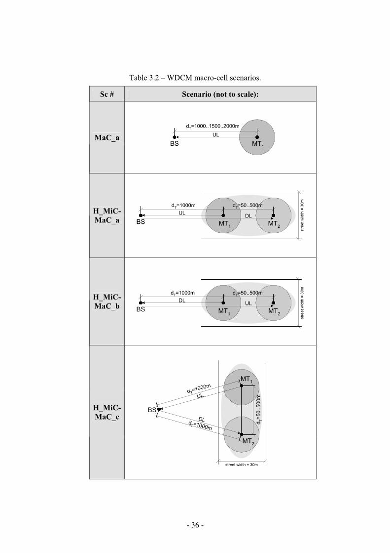
- 36 -

Table 3.2 – WDCM macro-cell scenarios.

Sc # Scenario (not to scale):

MaC_a

MT1BS

dT=1000..1500..2000mUL

H_MiC-MaC_a

MT1BS

dT=1000mUL

MT2

DL

stre

et w

idth

= 3

0mdT=50..500m

H_MiC-MaC_b

MT1BS

DL

MT2

ULst

reet

wid

th =

30mdT=50..500mdT=1000m

H_MiC-MaC_c

MT1

MT2

BS

street width = 30m

dT=1000m

d T=50

..500

m

dT=1000m

DL

UL

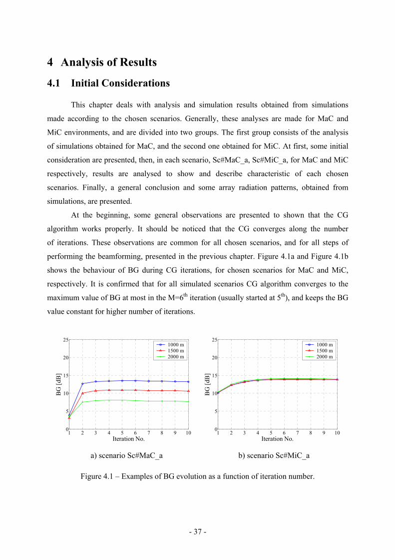
- 37 -

4 Analysis of Results

4.1 Initial Considerations This chapter deals with analysis and simulation results obtained from simulations

made according to the chosen scenarios. Generally, these analyses are made for MaC and

MiC environments, and are divided into two groups. The first group consists of the analysis

of simulations obtained for MaC, and the second one obtained for MiC. At first, some initial

consideration are presented, then, in each scenario, Sc#MaC_a, Sc#MiC_a, for MaC and MiC

respectively, results are analysed to show and describe characteristic of each chosen

scenarios. Finally, a general conclusion and some array radiation patterns, obtained from

simulations, are presented.

At the beginning, some general observations are presented to shown that the CG

algorithm works properly. It should be noticed that the CG converges along the number

of iterations. These observations are common for all chosen scenarios, and for all steps of

performing the beamforming, presented in the previous chapter. Figure 4.1a and Figure 4.1b

shows the behaviour of BG during CG iterations, for chosen scenarios for MaC and MiC,

respectively. It is confirmed that for all simulated scenarios CG algorithm converges to the

maximum value of BG at most in the M=6th iteration (usually started at 5th), and keeps the BG

value constant for higher number of iterations.

1 2 3 4 5 6 7 8 9 100

5

10

15

20

25

Iteration No.

BG

[dB

]

1000 m1500 m2000 m

1 2 3 4 5 6 7 8 9 100

5

10

15

20

25

Iteration No.

BG

[dB

]

1000 m1500 m2000 m

a) scenario Sc#MaC_a b) scenario Sc#MiC_a

Figure 4.1 – Examples of BG evolution as a function of iteration number.

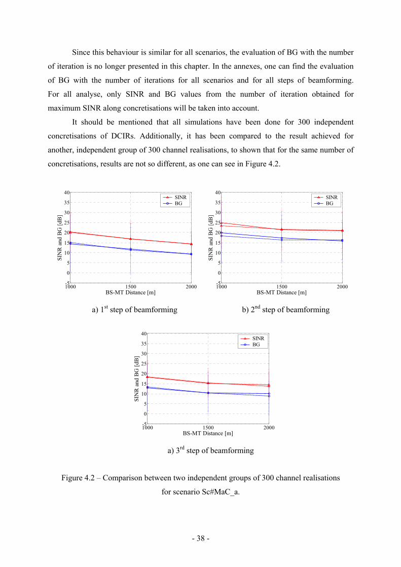
- 38 -

Since this behaviour is similar for all scenarios, the evaluation of BG with the number

of iteration is no longer presented in this chapter. In the annexes, one can find the evaluation

of BG with the number of iterations for all scenarios and for all steps of beamforming.

For all analyse, only SINR and BG values from the number of iteration obtained for

maximum SINR along concretisations will be taken into account.

It should be mentioned that all simulations have been done for 300 independent

concretisations of DCIRs. Additionally, it has been compared to the result achieved for

another, independent group of 300 channel realisations, to shown that for the same number of

concretisations, results are not so different, as one can see in Figure 4.2.

1000 1500 2000-5

0

5

10

15

20

25

30

35

40

BS-MT Distance [m]

SIN

R a

nd B

G [d

B]

SINRBG

1000 1500 2000-5

0

5

10

15

20

25

30

35

40

BS-MT Distance [m]

SIN

R a

nd B

G [d

B]

SINRBG

a) 1st step of beamforming b) 2nd step of beamforming

1000 1500 2000-5

0

5

10

15

20

25

30

35

40

BS-MT Distance [m]

SIN

R a

nd B

G [d

B]

SINRBG

a) 3rd step of beamforming

Figure 4.2 – Comparison between two independent groups of 300 channel realisations

for scenario Sc#MaC_a.

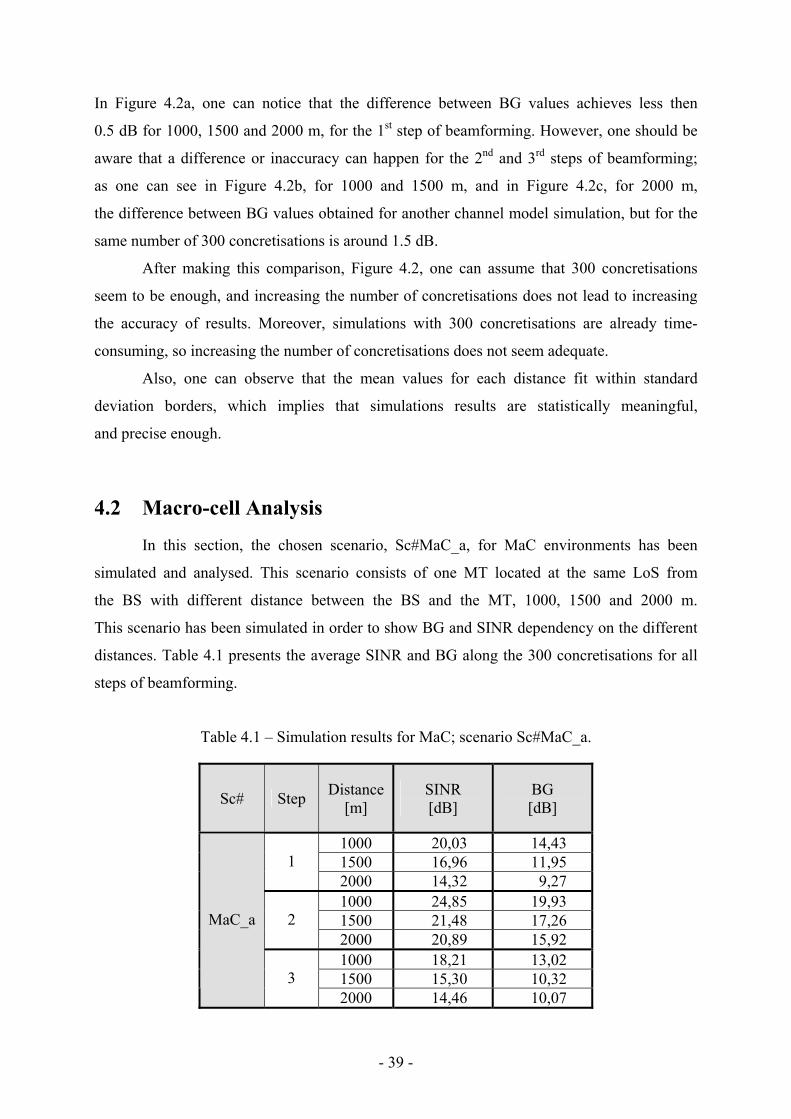
- 39 -

In Figure 4.2a, one can notice that the difference between BG values achieves less then

0.5 dB for 1000, 1500 and 2000 m, for the 1st step of beamforming. However, one should be

aware that a difference or inaccuracy can happen for the 2nd and 3rd steps of beamforming;

as one can see in Figure 4.2b, for 1000 and 1500 m, and in Figure 4.2c, for 2000 m,

the difference between BG values obtained for another channel model simulation, but for the

same number of 300 concretisations is around 1.5 dB.

After making this comparison, Figure 4.2, one can assume that 300 concretisations

seem to be enough, and increasing the number of concretisations does not lead to increasing

the accuracy of results. Moreover, simulations with 300 concretisations are already time-

consuming, so increasing the number of concretisations does not seem adequate.

Also, one can observe that the mean values for each distance fit within standard

deviation borders, which implies that simulations results are statistically meaningful,

and precise enough.

4.2 Macro-cell Analysis

In this section, the chosen scenario, Sc#MaC_a, for MaC environments has been

simulated and analysed. This scenario consists of one MT located at the same LoS from

the BS with different distance between the BS and the MT, 1000, 1500 and 2000 m.

This scenario has been simulated in order to show BG and SINR dependency on the different

distances. Table 4.1 presents the average SINR and BG along the 300 concretisations for all

steps of beamforming.

Table 4.1 – Simulation results for MaC; scenario Sc#MaC_a.

Sc# Step Distance [m]

SINR [dB]

BG [dB]

1000 20,03 14,43 1500 16,96 11,95 1 2000 14,32 9,27 1000 24,85 19,93 1500 21,48 17,26 2 2000 20,89 15,92 1000 18,21 13,02 1500 15,30 10,32

MaC_a

3 2000 14,46 10,07

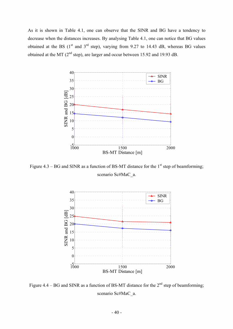
- 40 -

As it is shown in Table 4.1, one can observe that the SINR and BG have a tendency to

decrease when the distances increases. By analysing Table 4.1, one can notice that BG values

obtained at the BS (1st and 3rd step), varying from 9.27 to 14.43 dB, whereas BG values

obtained at the MT (2nd step), are larger and occur between 15.92 and 19.93 dB.

1000 1500 2000-5

0

5

10

15

20

25

30

35

40

BS-MT Distance [m]

SIN

R a

nd B

G [d

B]

SINRBG

Figure 4.3 – BG and SINR as a function of BS-MT distance for the 1st step of beamforming;

scenario Sc#MaC_a.

1000 1500 2000-5

0

5

10

15

20

25

30

35

40

BS-MT Distance [m]

SIN

R a

nd B

G [d

B]

SINRBG

Figure 4.4 – BG and SINR as a function of BS-MT distance for the 2nd step of beamforming;

scenario Sc#MaC_a.

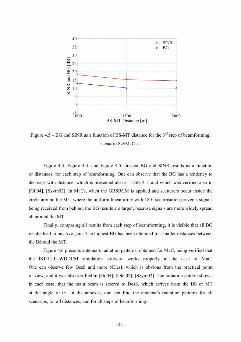
- 41 -

1000 1500 2000-5

0

5

10

15

20

25

30

35

40

BS-MT Distance [m]

SIN

R a

nd B

G [d

B]

SINRBG

Figure 4.5 – BG and SINR as a function of BS-MT distance for the 3rd step of beamforming;

scenario Sc#MaC_a.

Figure 4.3, Figure 4.4, and Figure 4.5, present BG and SINR results as a function

of distances, for each step of beamforming. One can observe that the BG has a tendency to

decrease with distance, which is presented also at Table 4.1, and which was verified also in

[Gil04], [Szym02]. In MaCs, when the GBSBCM is applied and scatterers occur inside the

circle around the MT, where the uniform linear array with 180° sectorisation prevents signals

being received from behind, the BG results are larger, because signals are more widely spread

all around the MT.

Finally, comparing all results from each step of beamforming, it is visible that all BG

results lead to positive gain. The highest BG has been obtained for smaller distances between

the BS and the MT.

Figure 4.6 presents antenna’s radiation patterns, obtained for MaC, being verified that

the IST/TUL–WDDCM simulation software works properly in the case of MaC.

One can observe few DesS and more NDesI, which is obvious from the practical point

of view, and it was also verified in [Gil04], [Olej02], [Szym02]. The radiation pattern shows,

in each case, that the main beam is steered to DesS, which arrives from the BS or MT

at the angle of 0°. In the annexes, one can find the antenna’s radiation patterns for all

scenarios, for all distances, and for all steps of beamforming.

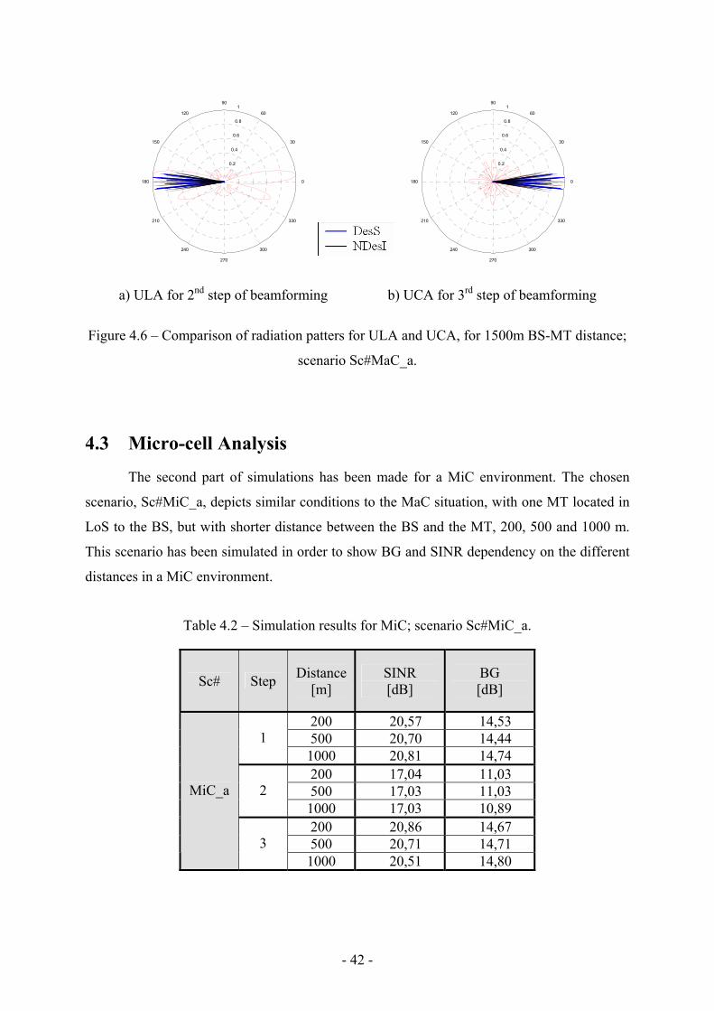
- 42 -

0.2

0.4

0.6

0.8

1

30

210

60

240

90

270

120

300

150

330

180 0

0.2

0.4

0.6

0.8

1

30

210

60

240

90

270

120

300

150

330

180 0

a) ULA for 2nd step of beamforming b) UCA for 3rd step of beamforming

Figure 4.6 – Comparison of radiation patters for ULA and UCA, for 1500m BS-MT distance;

scenario Sc#MaC_a.

4.3 Micro-cell Analysis

The second part of simulations has been made for a MiC environment. The chosen

scenario, Sc#MiC_a, depicts similar conditions to the MaC situation, with one MT located in

LoS to the BS, but with shorter distance between the BS and the MT, 200, 500 and 1000 m.

This scenario has been simulated in order to show BG and SINR dependency on the different

distances in a MiC environment.

Table 4.2 – Simulation results for MiC; scenario Sc#MiC_a.

Sc# Step Distance [m]

SINR [dB]

BG [dB]

200 20,57 14,53 500 20,70 14,44 1 1000 20,81 14,74 200 17,04 11,03 500 17,03 11,03 2 1000 17,03 10,89 200 20,86 14,67 500 20,71 14,71

MiC_a

3 1000 20,51 14,80

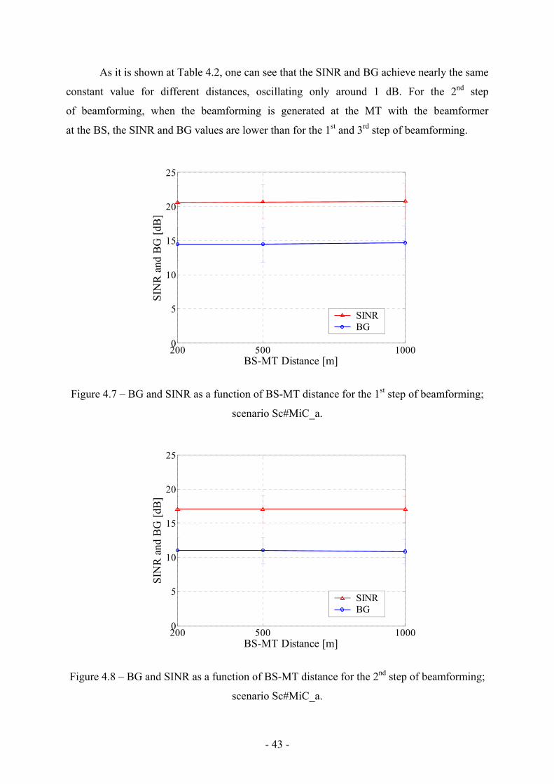
- 43 -

As it is shown at Table 4.2, one can see that the SINR and BG achieve nearly the same

constant value for different distances, oscillating only around 1 dB. For the 2nd step

of beamforming, when the beamforming is generated at the MT with the beamformer

at the BS, the SINR and BG values are lower than for the 1st and 3rd step of beamforming.

200 500 10000

5

10

15

20

25

BS-MT Distance [m]

SIN

R a

nd B

G [d

B]

SINRBG

Figure 4.7 – BG and SINR as a function of BS-MT distance for the 1st step of beamforming;

scenario Sc#MiC_a.

200 500 10000

5

10

15

20

25

BS-MT Distance [m]

SIN

R a

nd B

G [d

B]

SINRBG

Figure 4.8 – BG and SINR as a function of BS-MT distance for the 2nd step of beamforming;

scenario Sc#MiC_a.

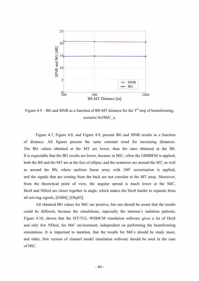
- 44 -

200 500 10000

5

10

15

20

25

BS-MT Distance [m]

SIN

R a

nd B

G [d

B]

SINRBG

Figure 4.9 – BG and SINR as a function of BS-MT distance for the 3rd step of beamforming;

scenario Sc#MiC_a.

Figure 4.7, Figure 4.8, and Figure 4.9, present BG and SINR results as a function

of distance. All figures present the same constant trend for increasing distances.

The BG values obtained at the MT are lower, than the ones obtained at the BS.

It is expectable that the BG results are lower, because in MiC, when the GBSBEM is applied,

both the BS and the MT are at the foci of ellipse, and the scatterers are around the MT, as well

as around the BS, where uniform linear array with 180° sectorisation is applied,

and the signals that are coming from the back are not consider at the MT array. Moreover,

from the theoretical point of view, the angular spread is much lower at the MiC,

DesS and NDesI are closer together in angle, which makes the DesS harder to separate from

all arriving signals, [Gil04], [Olej02].

All obtained BG values for MiC are positive, but one should be aware that the results

could be different, because the simulations, especially the antenna’s radiation patterns,

Figure 4.10, shown that the IST/TUL–WDDCM simulation software gives a lot of DesS

and only few NDesI, for MiC environment, independent on performing the beamforming

simulations. It is important to mention, that the results for MiCs should be study more,

and older, first version of channel model simulation software should be used in the case

of MiC.

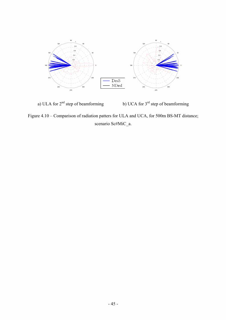
- 45 -

0.2

0.4

0.6

0.8

1

30

210

60

240

90

270

120

300

150

330

180 0

0.2

0.4

0.6

0.8

1

30

210

60

240

90

270

120

300

150

330

180 0

a) ULA for 2nd step of beamforming b) UCA for 3rd step of beamforming

Figure 4.10 – Comparison of radiation patters for ULA and UCA, for 500m BS-MT distance;

scenario Sc#MiC_a.

- 46 -

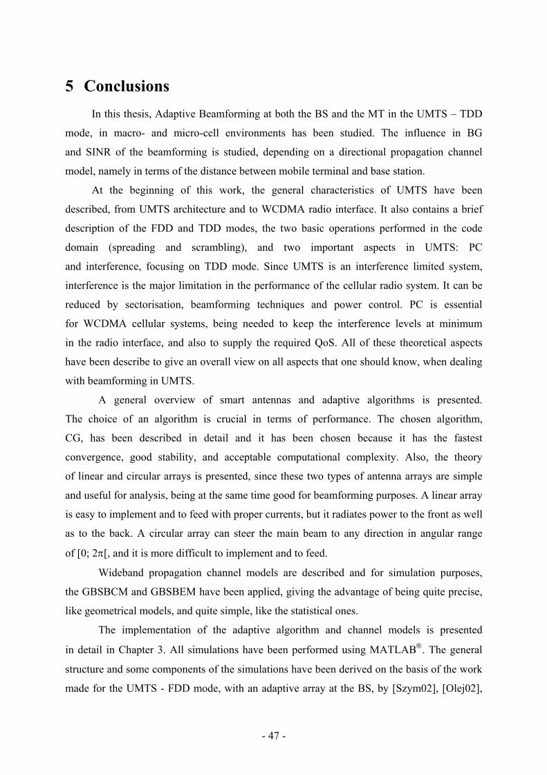
- 47 -

5 Conclusions In this thesis, Adaptive Beamforming at both the BS and the MT in the UMTS – TDD

mode, in macro- and micro-cell environments has been studied. The influence in BG

and SINR of the beamforming is studied, depending on a directional propagation channel

model, namely in terms of the distance between mobile terminal and base station.

At the beginning of this work, the general characteristics of UMTS have been

described, from UMTS architecture and to WCDMA radio interface. It also contains a brief

description of the FDD and TDD modes, the two basic operations performed in the code

domain (spreading and scrambling), and two important aspects in UMTS: PC

and interference, focusing on TDD mode. Since UMTS is an interference limited system,

interference is the major limitation in the performance of the cellular radio system. It can be

reduced by sectorisation, beamforming techniques and power control. PC is essential

for WCDMA cellular systems, being needed to keep the interference levels at minimum

in the radio interface, and also to supply the required QoS. All of these theoretical aspects

have been describe to give an overall view on all aspects that one should know, when dealing

with beamforming in UMTS.

A general overview of smart antennas and adaptive algorithms is presented.

The choice of an algorithm is crucial in terms of performance. The chosen algorithm,

CG, has been described in detail and it has been chosen because it has the fastest

convergence, good stability, and acceptable computational complexity. Also, the theory

of linear and circular arrays is presented, since these two types of antenna arrays are simple

and useful for analysis, being at the same time good for beamforming purposes. A linear array

is easy to implement and to feed with proper currents, but it radiates power to the front as well

as to the back. A circular array can steer the main beam to any direction in angular range

of [0; 2π[, and it is more difficult to implement and to feed.

Wideband propagation channel models are described and for simulation purposes,

the GBSBCM and GBSBEM have been applied, giving the advantage of being quite precise,

like geometrical models, and quite simple, like the statistical ones.

The implementation of the adaptive algorithm and channel models is presented

in detail in Chapter 3. All simulations have been performed using MATLAB. The general

structure and some components of the simulations have been derived on the basis of the work

made for the UMTS - FDD mode, with an adaptive array at the BS, by [Szym02], [Olej02],

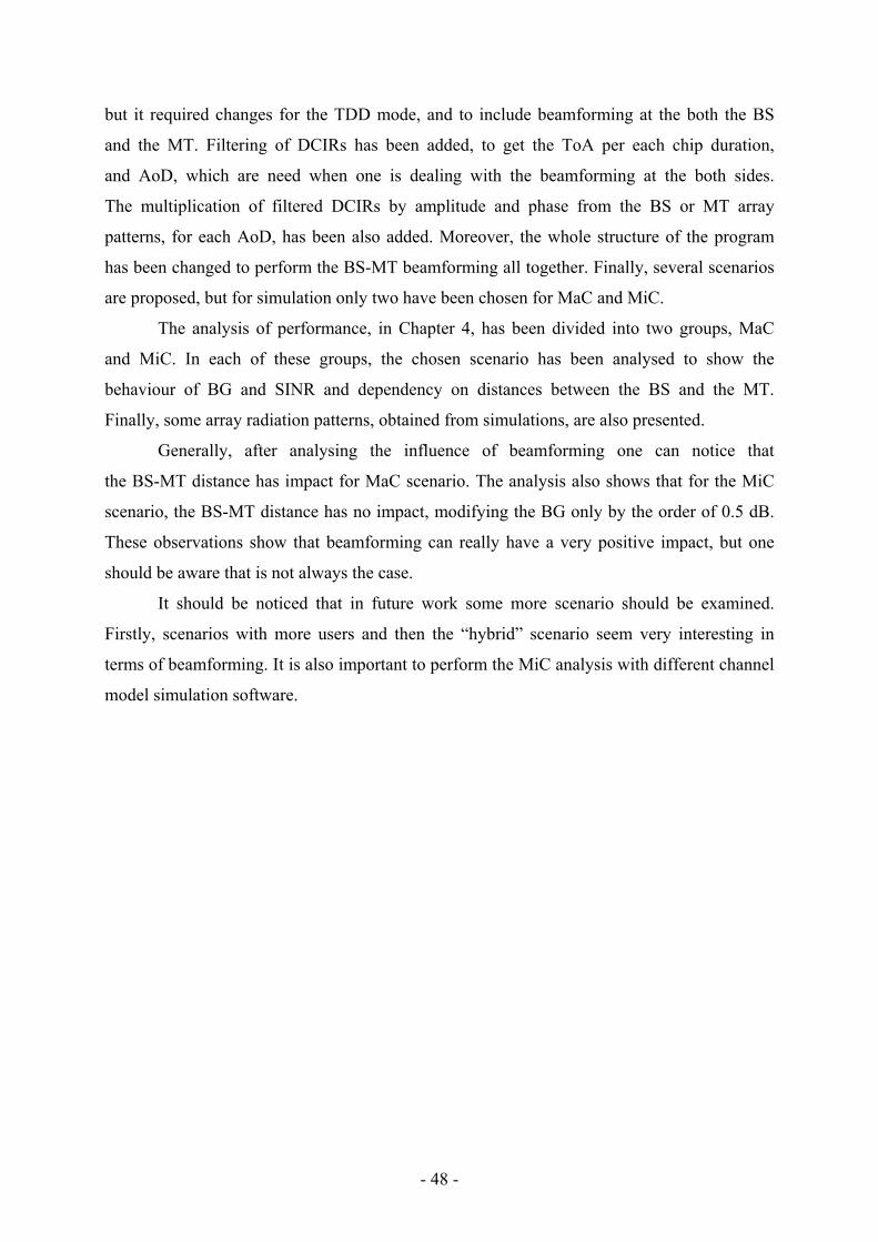
- 48 -

but it required changes for the TDD mode, and to include beamforming at the both the BS

and the MT. Filtering of DCIRs has been added, to get the ToA per each chip duration,

and AoD, which are need when one is dealing with the beamforming at the both sides.

The multiplication of filtered DCIRs by amplitude and phase from the BS or MT array

patterns, for each AoD, has been also added. Moreover, the whole structure of the program

has been changed to perform the BS-MT beamforming all together. Finally, several scenarios

are proposed, but for simulation only two have been chosen for MaC and MiC.

The analysis of performance, in Chapter 4, has been divided into two groups, MaC

and MiC. In each of these groups, the chosen scenario has been analysed to show the

behaviour of BG and SINR and dependency on distances between the BS and the MT.

Finally, some array radiation patterns, obtained from simulations, are also presented.

Generally, after analysing the influence of beamforming one can notice that

the BS-MT distance has impact for MaC scenario. The analysis also shows that for the MiC

scenario, the BS-MT distance has no impact, modifying the BG only by the order of 0.5 dB.

These observations show that beamforming can really have a very positive impact, but one

should be aware that is not always the case.

It should be noticed that in future work some more scenario should be examined.

Firstly, scenarios with more users and then the “hybrid” scenario seem very interesting in

terms of beamforming. It is also important to perform the MiC analysis with different channel

model simulation software.

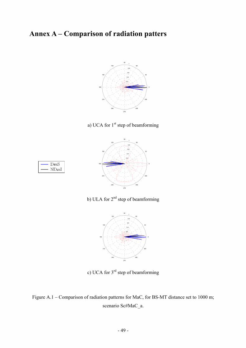
- 49 -

Annex A – Comparison of radiation patters

0.2

0.4

0.6

0.8

1

30

210

60

240

90

270

120

300

150

330

180 0

a) UCA for 1st step of beamforming

0.2

0.4

0.6

0.8

1

30

210

60

240

90

270

120

300

150

330

180 0

b) ULA for 2nd step of beamforming

0.2

0.4

0.6

0.8

1

30

210

60

240

90

270

120

300

150

330

180 0

c) UCA for 3rd step of beamforming

Figure A.1 – Comparison of radiation patterns for MaC, for BS-MT distance set to 1000 m;

scenario Sc#MaC_a.

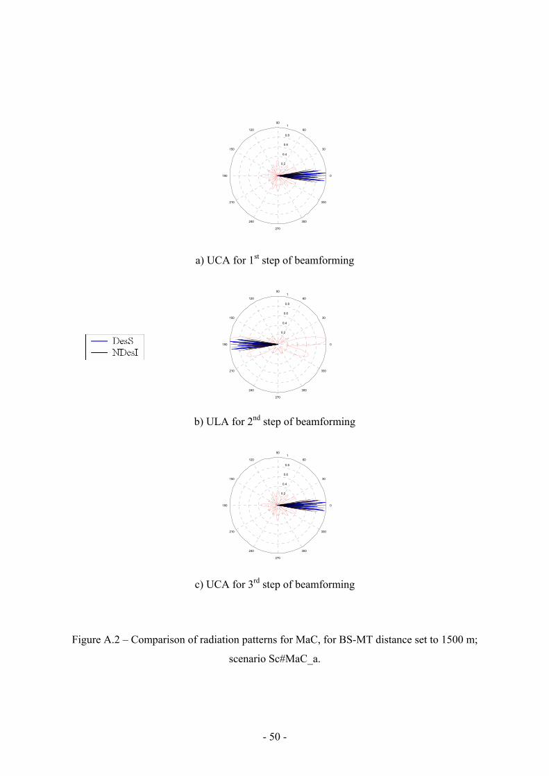
- 50 -

0.2

0.4

0.6

0.8

1

30

210

60

240

90

270

120

300

150

330

180 0


0.2

0.4

0.6

0.8

1

30

210

60

240

90

270

120

300

150

330

180 0


0.2

0.4

0.6

0.8

1

30

210

60

240

90

270

120

300

150

330

180 0



scenario Sc#MaC_a.

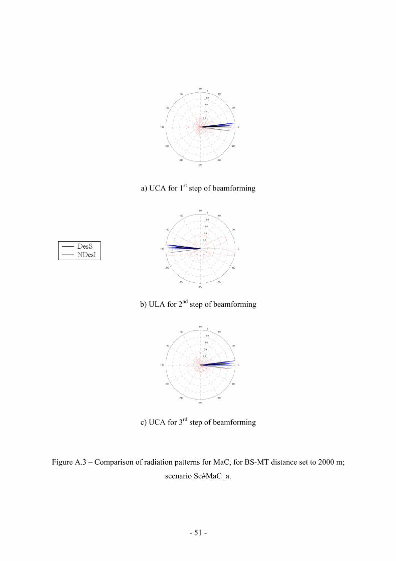
- 51 -

0.2

0.4

0.6

0.8

1

30

210

60

240

90

270

120

300

150

330

180 0


0.2

0.4

0.6

0.8

1

30

210

60

240

90

270

120

300

150

330

180 0


0.2

0.4

0.6

0.8

1

30

210

60

240

90

270

120

300

150

330

180 0



scenario Sc#MaC_a.

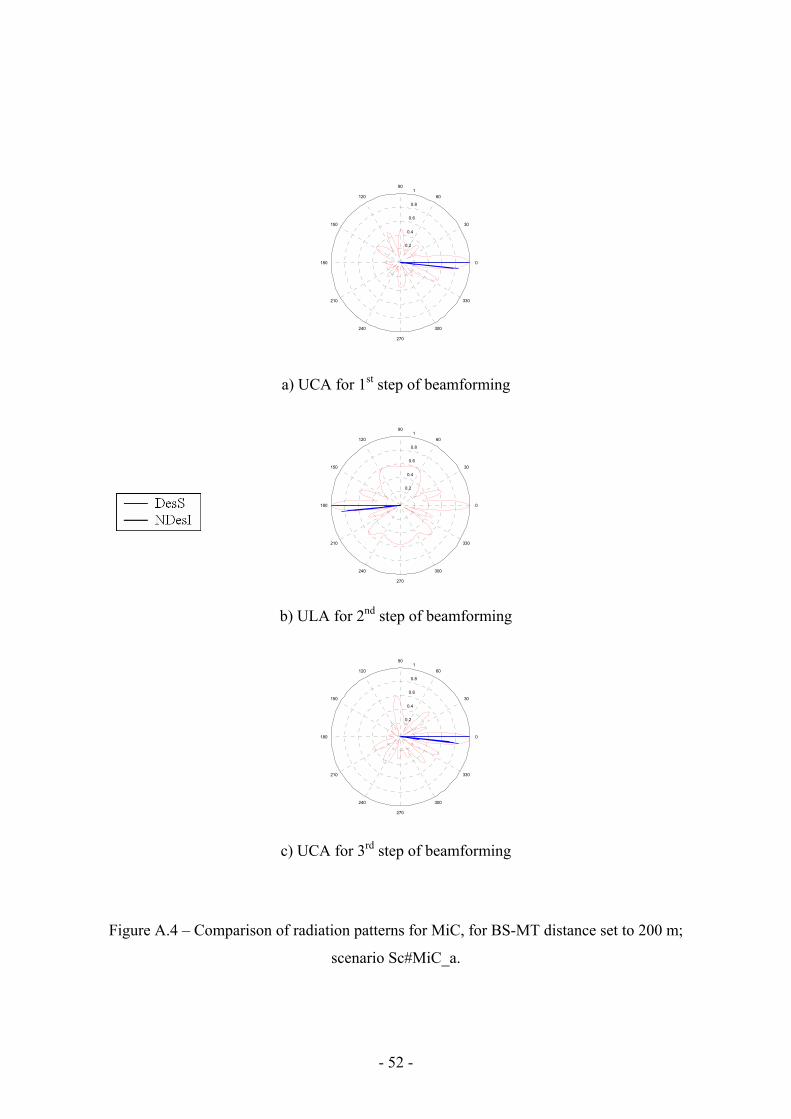
- 52 -

0.2

0.4

0.6

0.8

1

30

210

60

240

90

270

120

300

150

330

180 0


0.2

0.4

0.6

0.8

1

30

210

60

240

90

270

120

300

150

330

180 0


0.2

0.4

0.6

0.8

1

30

210

60

240

90

270

120

300

150

330

180 0


Figure A.4 – Comparison of radiation patterns for MiC, for BS-MT distance set to 200 m;

scenario Sc#MiC_a.

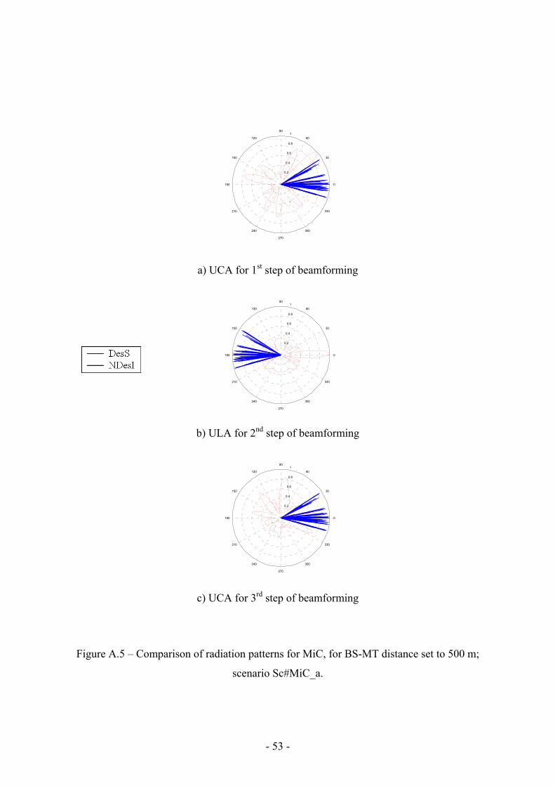
- 53 -

0.2

0.4

0.6

0.8

1

30

210

60

240

90

270

120

300

150

330

180 0


0.2

0.4

0.6

0.8

1

30

210

60

240

90

270

120

300

150

330

180 0


0.2

0.4

0.6

0.8

1

30

210

60

240

90

270

120

300

150

330

180 0



scenario Sc#MiC_a.

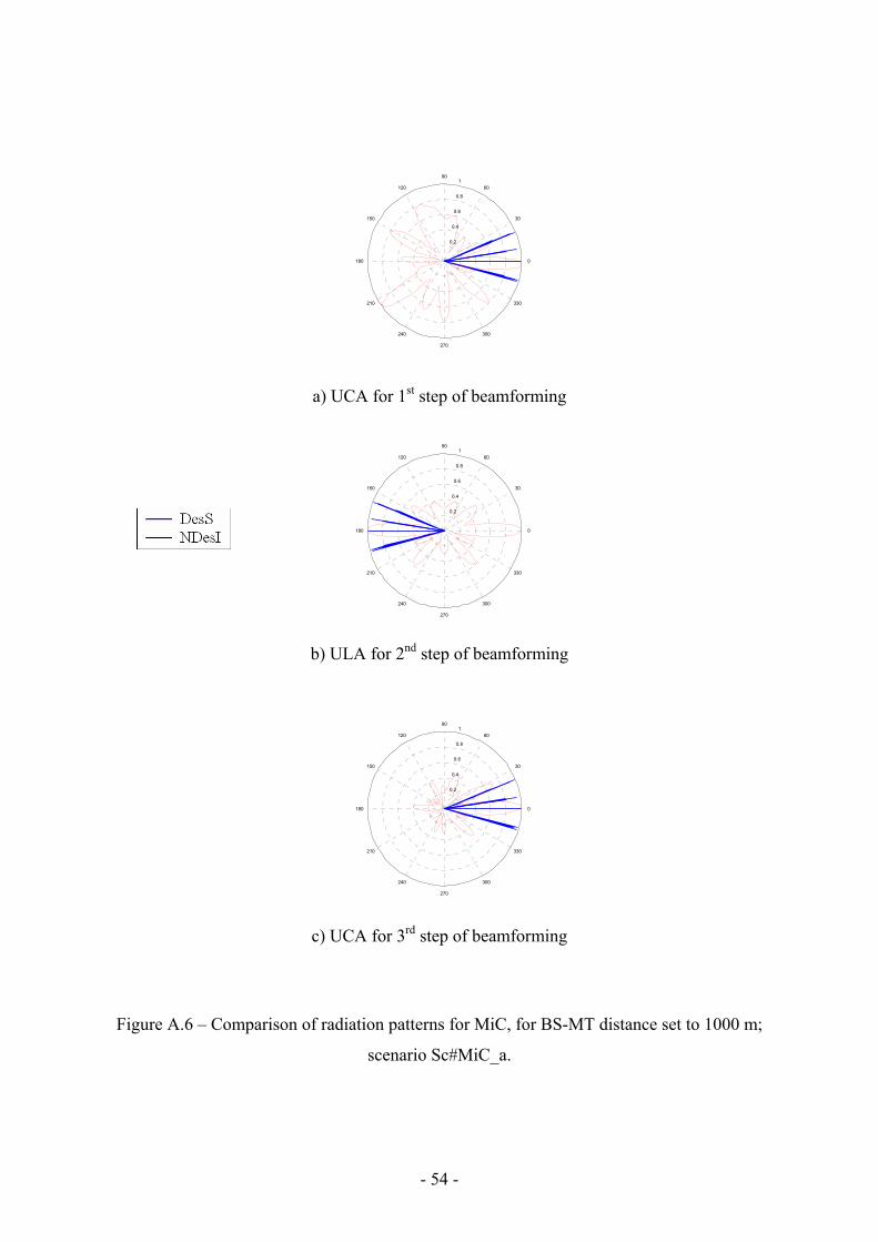
- 54 -

0.2

0.4

0.6

0.8

1

30

210

60

240

90

270

120

300

150

330

180 0


0.2

0.4

0.6

0.8

1

30

210

60

240

90

270

120

300

150

330

180 0


0.2

0.4

0.6

0.8

1

30

210

60

240

90

270

120

300

150

330

180 0



scenario Sc#MiC_a.

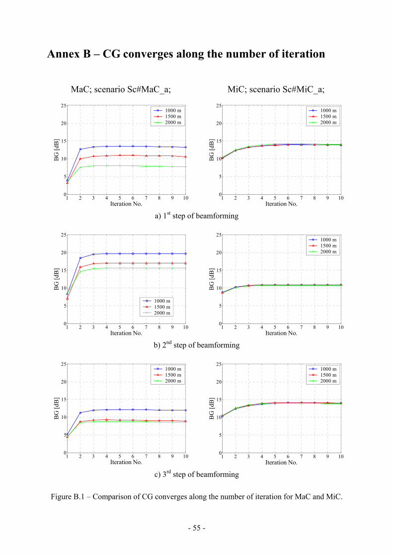
- 55 -

Annex B – CG converges along the number of iteration

MaC; scenario Sc#MaC_a; MiC; scenario Sc#MiC_a;

1 2 3 4 5 6 7 8 9 100

5

10

15

20

25

Iteration No.

BG

[dB

]

1000 m1500 m2000 m

1 2 3 4 5 6 7 8 9 100

5

10

15

20

25

Iteration No.B

G [d

B]

1000 m1500 m2000 m

a) 1st step of beamforming

1 2 3 4 5 6 7 8 9 100

5

10

15

20

25

Iteration No.

BG

[dB

]

1000 m1500 m2000 m

1 2 3 4 5 6 7 8 9 100

5

10

15

20

25

Iteration No.

BG

[dB

]

1000 m1500 m2000 m

b) 2nd step of beamforming

1 2 3 4 5 6 7 8 9 100

5

10

15

20

25

Iteration No.

BG

[dB

]

1000 m1500 m2000 m

1 2 3 4 5 6 7 8 9 100

5

10

15

20

25

Iteration No.

BG

[dB

]

1000 m1500 m2000 m

c) 3rd step of beamforming

Figure B.1 – Comparison of CG converges along the number of iteration for MaC and MiC.

- 56 -

- 57 -

References

[3GPP03a] 3GPP, Physical layer - General description, Technical Specification 25.201

v6.0.0, Dec. 2003 (http://www.3gpp.org).

[3GPP03b] 3GPP, Spreading and modulation (FDD), Technical Specification 25.213

v6.0.0, Dec. 2003 (http://www.3gpp.org).

[Bagh99] Baghaie,R., “Systolic implementation of sample-by-sample conjugate

gradient algorithm”, in Proc. of FINSIG’99 – IEEE Finish Signal Processing

Symposium, Oulu, Finland, May 1999.

[Bala97] Balanis,C.A., Antenna Theory: analysis and design, John Wiley & Sons,

New York, USA, 1997.

[ChKi92] Choi,S. and Kim,D.H., “Adaptive Antenna Array Utilising the Conjugate

Gradient Method for Compensation of Multipath Fading in a Land Mobile

Communication”, in Proc. of VTC’92 – 42nd IEEE Vehicular Technology

Conference, Denver, CO, USA, May 1992.

[DGVC03] Debbah,M., Gil,J.M., Venes,J., Cardoso,F., Marques,G. and Correia,L.M.,

Final report on channel models, IST-FLOWS Project, Deliverable D13,

EC-IST Office, Brussels, Belgium, Sep. 2003, (http://www.flows-ist.org).

[Gil04] Gil,J.M., Dependencies of Adaptive Beamforming on the Propagation

Channel in Wideband Mobile Communications, PhD. Thesis, Instituto

Superior Técnico, Technical University of Lisbon, Lisbon, Portugal,

June 2004.

[GiCo02] Gil,J.M. and Correia,L.M., Dependence of Adaptive Beamforming

Performance on Directional Channel Macro-Cell Scenarios for UMTS,

COST 273, Temporary Document TD(02)050, Espoo, Finland, May 2002.

- 58 -

[GiCo03] Gil,J.M. and Correia,L.M., “Adaptive Beamforming Dependencies on

Wideband and Directional Propagation Characteristics in Micro- and Macro-

Cell UMTS Scenarios”, in Proc. of PIMRC’2003 – 14th IEEE International

Symposium on Personal, Indoor and Mobile Communications, Beijing,

China, Sep. 2003.

[GiMC01] Gil,J.M., Mendez,J., and Correia,L.M., “Comparison of Recursive Least

Squares and Conjugate Gradient Applied to Adaptive Beamforming in

UMTS”, in Proc. of IST Mobile Communications Summit 2001, Barcelona,

Spain, Sep. 2001.

[Goda97] Godara,L.C., “Application of Antenna Arrays to Mobile Communications,

Part II: Beam-forming and Direction-of-Arrival Considerations”, Proc. of the

IEEE, Vol. 85, No. 8, Aug. 1997, pp. 1193-1245.

[HeBK99] Hernandez,R.I., Baghaie,R. and Kettunen,K., “Implementation of Gram-

Schmidt conjugate direction and conjugate gradient algorithms”, in Proc. of

FINSIG’99 – IEEE Finish Signal Processing Symposium, Oulu, Finland,

May 1999.

[Hera00] Herault,L., Project Presentation Report, IST-ASILUM project,

Deliverable D0.2, EC-IST Office, Brussels, Belgium, Apr. 2000,

(http://www.nari.ee.ethz.ch/~asilum/).

[HoTo01] Holma,H. and Toskala,A., WCDMA for UMTS, John Wiley & Sons,

Chichester, UK, 2001.

[KALN01] Kaaranen,H., Ahtiainen,A., Laitinen,L., Naghian,S. and Niemi,V.,

UMTS Networks, John Wiley & Sons, Chichester, UK, 2001.

[LiLo96] Litva,J. and Lo,T.K., Digital Beamforming in Wireless Communications,

Artech House, Norwood, MA, USA, 1996.

[LiRa99] Liberti,J.C. and Rappaport,T.S., Smart Antennas for Wireless

Communications: IS-95 and Third Generation CDMA Applications, Prentice

Hall, Upper Saddle River, NJ, USA, 1999.

- 59 -

[MaCo01] Marques,M.G. and Correia,L.M., “A Wideband Directional Channel Model

for UMTS Micro-cells”, in Proc. of PIMRC’01 – 12th IEEE Personal, Indoor

and Mobile Radio Communications Conference, San Diego, CA, USA,

Sep. 2001.

[Marq01] Marques,M.G., A Wideband Directional Model for Micro-Cells in UMTS,

M.Sc. Thesis, Instituto Superior Técnico, Technical University of Lisbon,

Lisbon, Portugal, 2001.

[Olej02] Olejniczak,J., Impact of the directional channel in adaptive beamforming for

UMTS-FDD in micro-cells, Graduation Project, Instituto Superior Técnico,

Technical University of Lisbon, Lisbon, Portugal, 2002.

[Szym02] Szymański,T., Impact of the directional channel in adaptive beamforming for

UMTS-FDD in macro-cells, Graduation Project, Instituto Superior Técnico,

Technical University of Lisbon, Lisbon, Portugal, 2002.

[VeBu88] Van Veen,B.D. and Buckley,K.M., ”Beamforming: A Versatile Approach to

Spatial Filtering”, IEEE Acoustics, Speech and Signal Processing Magazine,

Vol. 5, No. 2, Apr. 1988, pp. 4-24.

[ZoMa00] Zollinger,E. and Marques,G., Wideband Directional Channel Model and

Measurement Campaign, IST-ASILUM Project, Deliverable D2.1, IST

Central Office, Brussels, Belgium, Nov. 2000.

Documents

COMBINING ADAPTIVE ANTENNAS AT BOTH THE …grow.tecnico.ulisboa.pt/wp-content/uploads/2014/01/MScThesis...combining adaptive antennas at both the base station and the mobile terminal