Spectral Clustering Presented by Eldad Rubinstein

Based on a Tutorial by Ulrike von Luxburg TAU Big Data Processing Seminar December 14, 2014

What are we going to talk about?

• Introduction

– Clustering and k-Means

– Kernel methods

• Spectral Clustering

– Similarity graphs

– The algorithm itself

• Motivations

– Graph cut

– Random walk

• Examples and Summary

2

Clustering

• Cluster in Hebrew – אשכול or צביר

• Grouping “similar” objects into sets

– Maximize similarity within a category

– Minimize similarity between categories

• This is an unsupervised learning task

• Many applications, for instance:

– Image Segmentation

– Finding communities in social networks

3

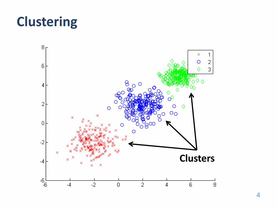
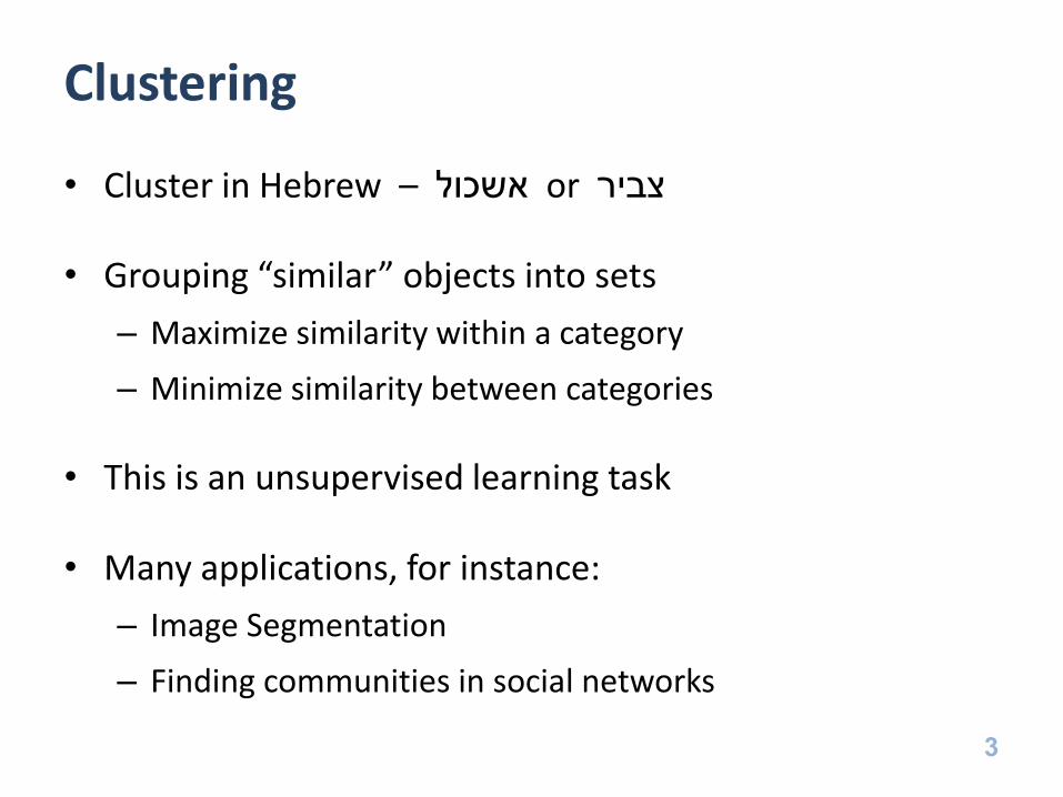
Clustering

4

Clusters

k-Means

• Popular clustering algorithm

• Definitions

– Dataset points

– Clusters with centroids

• NP-hard objective function

5

For each point, choose

the closest centroid

Minimize over centroid

locations

k-Means

6

• Input: data and k (number of clusters)

• Initialize: Choose centroids

• Iterate:

– Put each point in the cluster of the closest centroid

– Move each centroid to the mean of its cluster points

k-Means Disadvantages

7

• It doesn’t always reach the NP-hard objective

• It is unclear how to initialize the centroids

• Doesn’t work when the centroid assumption doesn’t hold:

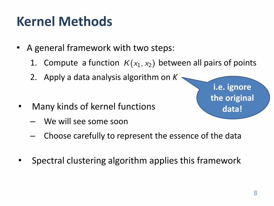
Kernel Methods

• A general framework with two steps:

1. Compute a function between all pairs of points

2. Apply a data analysis algorithm on K

• Many kinds of kernel functions

– We will see some soon

– Choose carefully to represent the essence of the data

• Spectral clustering algorithm applies this framework

8

i.e. ignore the original

data!

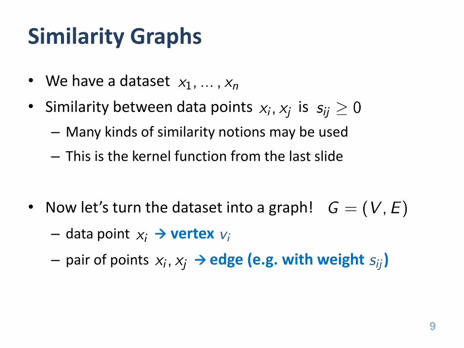
Similarity Graphs

• We have a dataset

• Similarity between data points is

– Many kinds of similarity notions may be used

– This is the kernel function from the last slide

• Now let’s turn the dataset into a graph!

– data point vertex

– pair of points edge (e.g. with weight )

9

Similarity Graphs (Examples)

• e -Neighborhood Graphs

– Connect all point whose pairwise distance

• k-Nearest Neighbors Graphs

– If x1 is one of the k nearest neighbors of x2 , connect them

– Should make it symmetric

• Fully connected graphs

– Important example – Gaussian (RBF) kernel

10

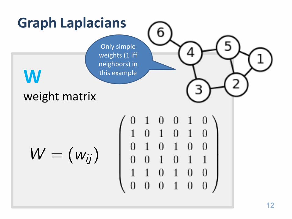
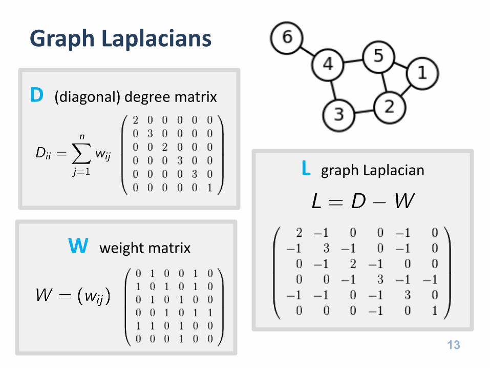
Graph Laplacians

11

D

(diagonal) degree matrix

Graph Laplacians

12

W weight matrix

Only simple weights (1 iff neighbors) in this example

Graph Laplacians

13

D (diagonal) degree matrix

L graph Laplacian

W weight matrix

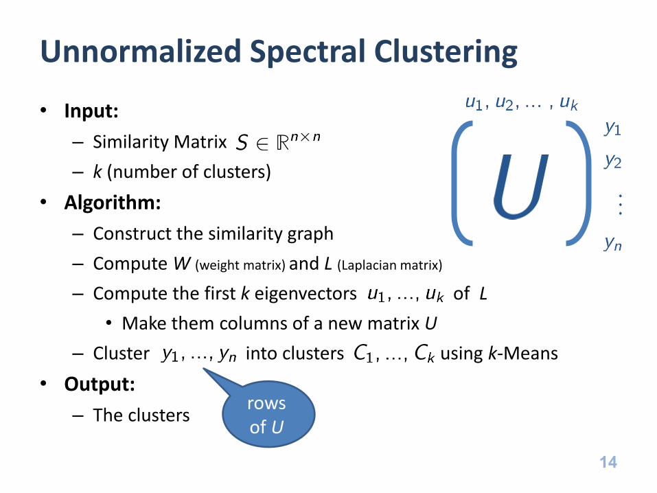
Unnormalized Spectral Clustering

• Input:

– Similarity Matrix

– k (number of clusters)

• Algorithm:

– Construct the similarity graph

– Compute W (weight matrix) and L (Laplacian matrix)

– Compute the first k eigenvectors of L

• Make them columns of a new matrix U

– Cluster into clusters using k-Means

• Output:

– The clusters

14

rows of U

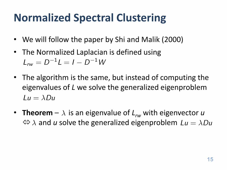
Normalized Spectral Clustering

• We will follow the paper by Shi and Malik (2000)

• The Normalized Laplacian is defined using

• The algorithm is the same, but instead of computing the eigenvalues of L we solve the generalized eigenproblem

• Theorem – is an eigenvalue of Lrw with eigenvector u and u solve the generalized eigenproblem

15

Example

16

• k-NN similarity

• normalized (1st row) and unnormalized (2nd row)

1-d data

Example

17

• Gaussian similarity function

• normalized (1st row) and unnormalized (2nd row)

1-d data

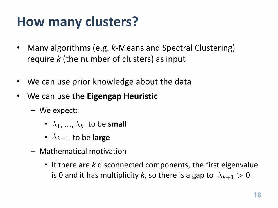
How many clusters?

18

• Many algorithms (e.g. k-Means and Spectral Clustering) require k (the number of clusters) as input

• We can use prior knowledge about the data

• We can use the Eigengap Heuristic

– We expect:

• to be small

• to be large

– Mathematical motivation

• If there are k disconnected components, the first eigenvalue is 0 and it has multiplicity k, so there is a gap to

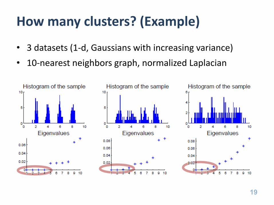
How many clusters? (Example)

19

• 3 datasets (1-d, Gaussians with increasing variance)

• 10-nearest neighbors graph, normalized Laplacian

Graph Cut Analysis

• Clustering Graph Min Cut

• We define cut using

– Where

• But we want all sets to be reasonably large

– So we’ll use a different objective:

• We want to minimize this function

20

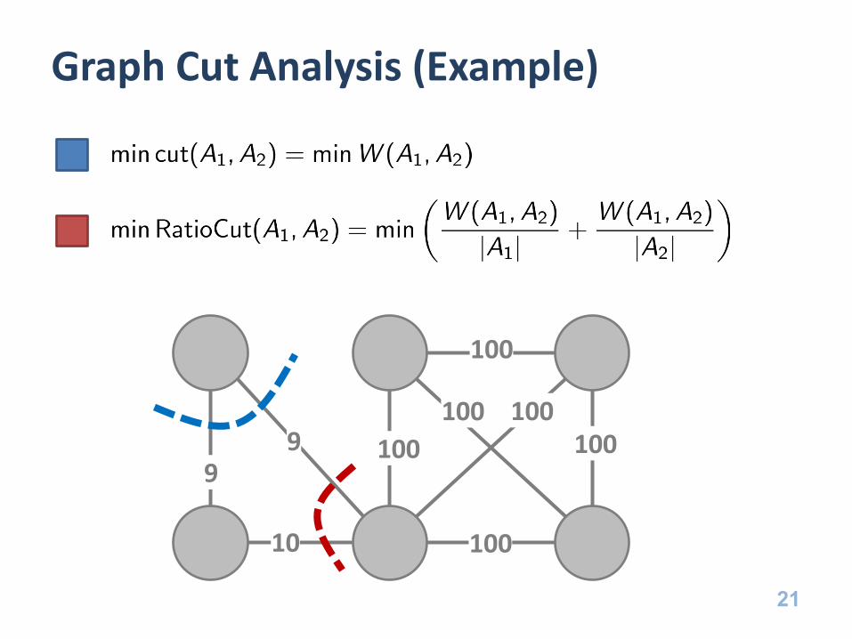
Graph Cut Analysis (Example)

21

9 9

10

100

100

100

100 100 100

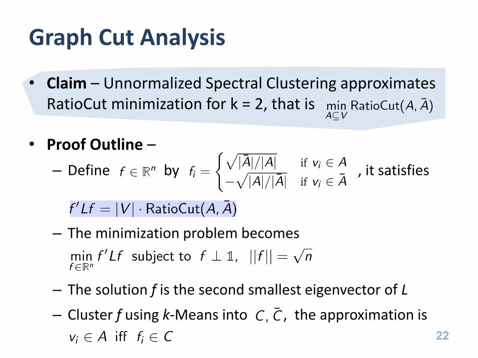
Graph Cut Analysis

• Claim – Unnormalized Spectral Clustering approximates RatioCut minimization for k = 2, that is

• Proof Outline –

– Define by , it satisfies

– The minimization problem becomes

– The solution f is the second smallest eigenvector of L

– Cluster f using k-Means into , the approximation is

22

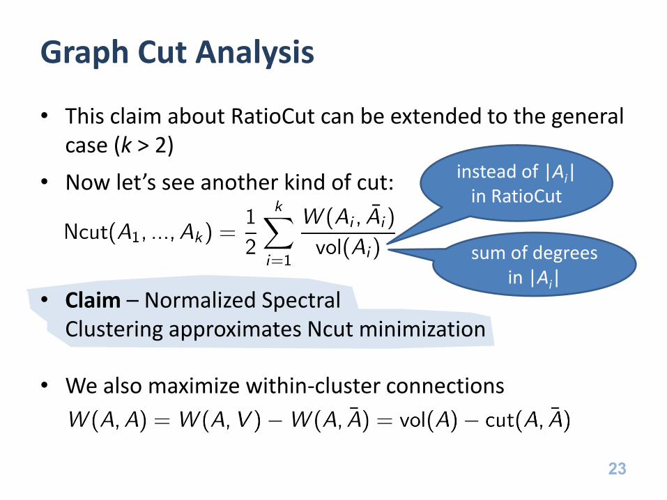
Graph Cut Analysis

• This claim about RatioCut can be extended to the general case (k > 2)

• Now let’s see another kind of cut:

• Claim – Normalized Spectral

Clustering approximates Ncut minimization

• We also maximize within-cluster connections

23

instead of |Ai| in RatioCut

sum of degrees in |Ai|

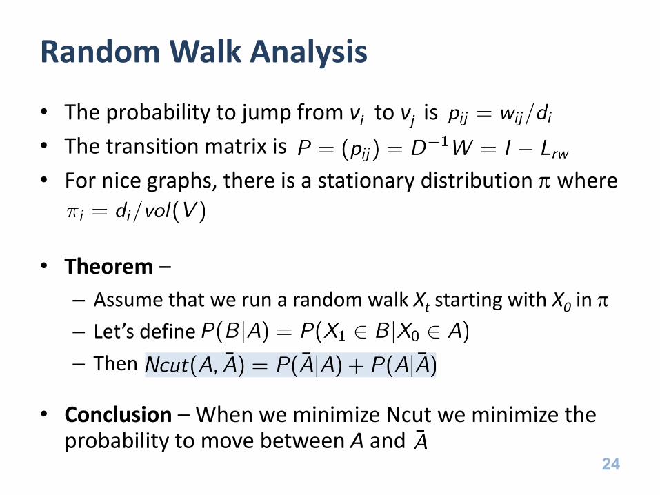
Random Walk Analysis

• The probability to jump from vi to vj is

• The transition matrix is

• For nice graphs, there is a stationary distribution p where

• Theorem –

– Assume that we run a random walk Xt starting with X0 in p

– Let’s define

– Then

• Conclusion – When we minimize Ncut we minimize the probability to move between A and

24

Toy Data Example

25

• Testing Spectral Clustering

– with toy data

– using Python + scikit-learn

• Create datasets (with two clusters)

• Cluster them using:

– Spectral Clustering with RBF (Gaussian) similarity matrix

– Spectral Clustering with 10 Nearest Neighbors connectivity matrix

– k-Means

Example Results

26

k-Means

Spectral Clustering (NN)

Spectral Clustering (RBF)

Image Segmentation Example

27

• Goal – Separating noisy circles

• Dataset – Image pixels

• Similarity Function – Gaussian kernel of the pixel gradients

Input Image Output Clusters

Summary

28

• Clustering is an important task

• We have seen two approaches to clustering

– k-Means – assumes that each cluster is around a centroid

– Spectral Clustering – Kernel + Graph-theoretic based

• Spectral clustering uses knowledge from spectral graph theory to analyze data

• Spectral Clustering can be justified

– Using graph cut point of view

– Using random walk point of view

Bibliography

29

• Spectral Clustering Tutorial by Ulrike von Luxburg

• Machine Learning Course Handouts by Shai Shalev-Shwartz

• Clustering web page from Python scikit-learn documentation (http://scikit-learn.org/stable/modules/clustering.html)

• Kernel Methods Presentation by Nello Cristianini

• Wikipedia (especially for illustrations and examples)

Questions?