A Non-Walrasian Labor Market and theEuropean Business Cycle

Francesco Zanetti∗

Boston College

May 2004

Abstract

This paper investigates to what extent a New Keynesian, mone-tary model with the addition of a microfounded, non-Walrasian labormarket based on union bargaining is able to replicate key aspects ofthe business cycle. The presence of a representative union offers anexplanation for two features of the cycle. First, it generates an en-dogenous mechanism which produces persistent responses of the econ-omy to both supply and demand shocks. Second, labor unionizationcauses a lower elasticity of marginal costs to output. This leads tolower inflation volatility. The model can replicate the negative cor-relation between productivity shocks and employment in the data.Model simulations show the superiority of the unionized frameworkin reproducing European business cycle statistics relative to a modelwith a competitive labor market.JEL: E24, E31, E32.Key Words: Trade Unions, Business Cycle, Inflation, Persistence.

∗I wish to thank Kit Baum, Chuck Carlstrom, Fabio Ghironi, Matteo Iacoviello, SusanaIranzo, Peter Ireland, Arthur Lewbel, Marco Maffezzoli, Mirco Soffritti, Richard Treschseminar participants at Boston College, Ente Einaudi, and Bank of England for usefulcomments. I thank the Ente Luigi Einaudi and the European Central Bank for hospitality.The usual disclaimer applies. Please address correspondence to: Francesco Zanetti, BostonCollege, Department of Economics, 140 Commonwealth Avenue, Chestnut Hill, MA 02467-3806. Fax:+1-617-552-2308. Email: zanettif@bc.edu.

1

1 Introduction

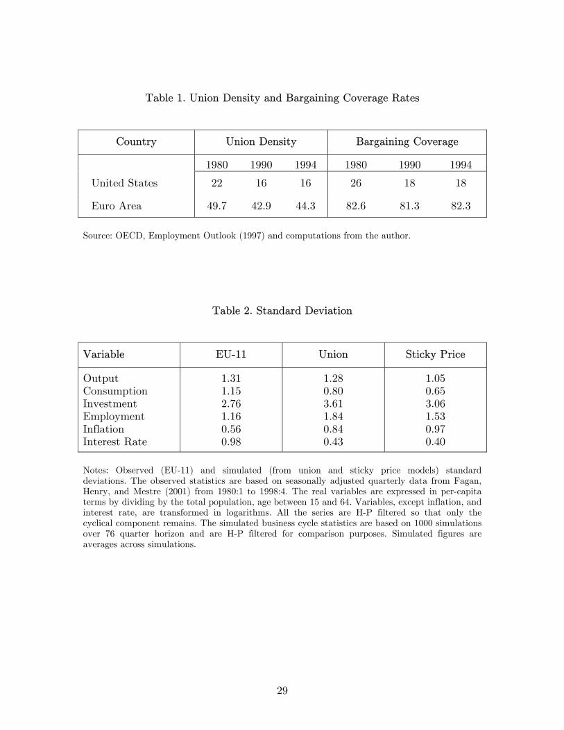
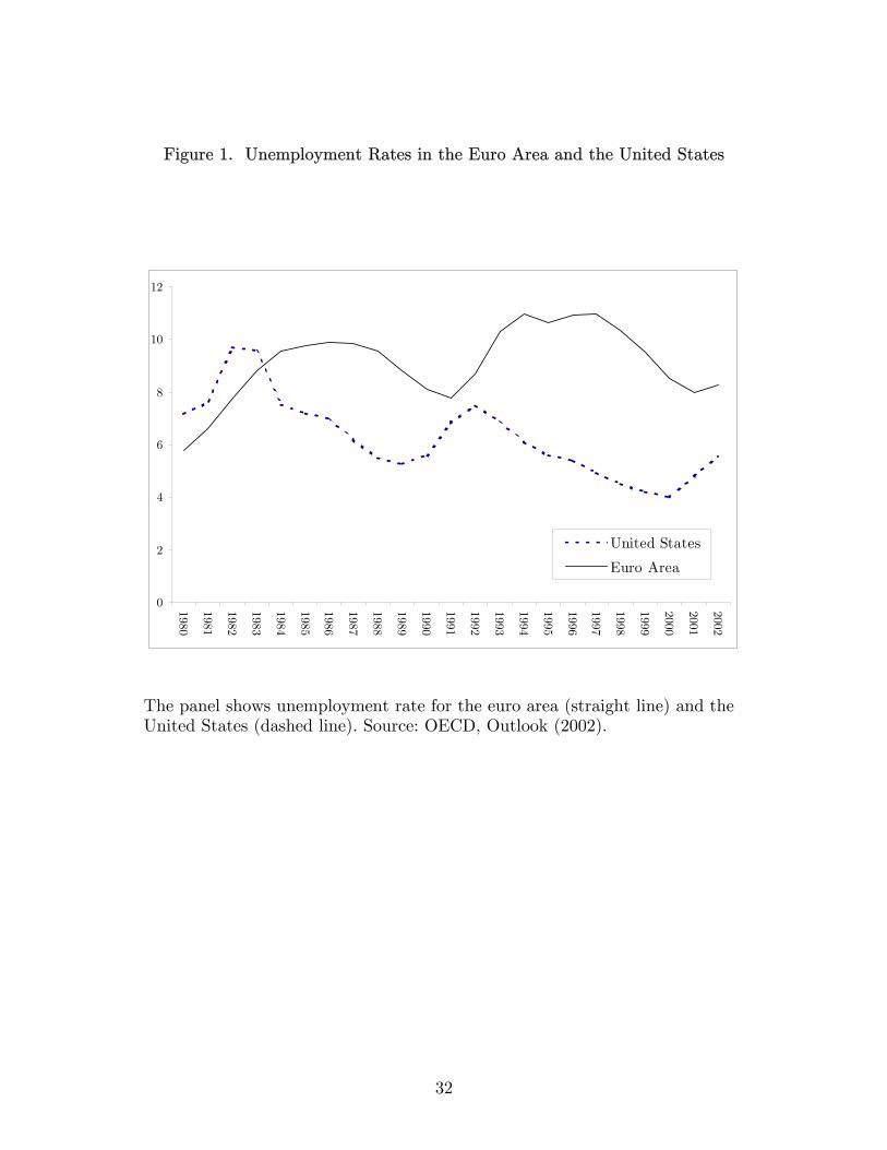
High unemployment rates have been a feature of the euro area countries forthe last two decades, despite the concern of the European Commission andnational governments. Figure 1 compares unemployment rates in the euroarea countries and in the United States. Although the timing of fluctuationsfor these economies is similar, amplitude and unemployment persistence havebeen considerably larger for the euro area.High unions density and coverage rates are striking features of the Euro-

pean labor market. Unionization is substantially more pervasive if comparedwith the American counterpart, as shown in Table 1. From these measures,we can infer a higher level of union power in Europe relative to the UnitedStates during the last two decades.These facts suggest that a perfectly competitive labor market may not be

the appropriate theoretical framework for the euro area, where countries aregenerally characterized by imperfections in the labor market and rigidities inthe economy. In this paper, I incorporate equilibrium unemployment throughunion bargaining in an otherwise standard New Keynesian monetary model.I then use the model to study the consequences of union bargaining on thebusiness cycle.The theoretical set up I introduce is characterized by an innovative New

Keynesian monetary model which encompasses departures from perfect com-petition in both labor and product markets. The structure of the labor mar-ket is non-Walrasian: Wages are set by the bargaining process between firmsand trade unions somewhere above the market-clearing level. This generatesunemployment as some individual workers are unable to sell as much laborservices as they wish to supply, given the established wages. Goods marketsare imperfectly competitive due to the presence of monopolistically competi-tive, intermediate goods-producing firms. The monetary authority conductsmonetary policy through interest rate setting in the form of a Taylor-typerule. Finally, I explicitly incorporate real and nominal rigidities, in the formof capital and price adjustment costs.The set up improves upon the previous literature in the following man-

ners. First, Hall (2000) stresses that variables’ persistence in the aftermathof shocks is a critical property of the data that standard neoclassical modelsfail to reproduce. He suggests that the inclusion of non-Walrasian featuresmay improve the replication of this feature of the business cycle. Alongthese lines, Maffezzoli (2001) shows that a real business cycle model with a

2

monopoly union has a comparative advantage over the Rogerson and Wright(1988) indivisible labor model in the replication of Italian business cycle sta-tistics. Nonetheless, his model cannot embed monetary policy shocks andis not able to generate appropriate persistence in reaction to supply shocks.Alexopoulos (2004) develops a shirking efficiency wage model which improvesthe replication of labor markets statistics but again fails to deliver an appro-priate degree of persistence. Dotsey and King (2001), building upon Chari,Kehoe, and McGrattan (2000), point out that standard sticky price mod-els are not able to account for the persistent response of output to demandshocks and they allow for a number of “supply side” features to improve theperformance of a standard sticky price model. In this paper, the introduc-tion of labor market bargaining into a standard sticky price model createsan endogenous mechanism based on lower wage volatility that independentlyintroduces persistence in response to both supply and demand shocks.Second, Bernanke and Gertler (1995), Christiano, Eichenbaum, and Evans

(1997), and Bernanke and Mihov (1998) offer evidence that inflation variesonly moderately in response to monetary policy shocks. Standard New Key-nesian sticky price models are not capable of capturing this feature of thebusiness cycle. In this set up a unionized labor market generates lower elastic-ity of marginal costs with respect to output, and this translates into moderateprice adjustments. This increases the level of price stickiness to changes inaggregate demand and diminishes inflation volatility.Third, recent contributions as Christiano and Eichenbaum (1992), Bernanke

and Gertler (1995), Bernanke and Mihov (1998), Shea (1998), Basu, Fernaldand Kimball (2002), Galì (1999), and Francis and Ramey (2003) point outa negative correlation between productivity shocks and employment. In linewith these studies, both the union and the baseline sticky price models ofthis paper are able to reproduce this feature due to the delayed reaction ofprices and production to technology shocks.Numerical simulations show that the presence of a non-Walrasian labor

market improves the ability of a standard sticky price model to replicate theEuropean business cycle relative to the standard model without monopolyunions. Attention is focused on the comparison between models and Eu-ropean statistics for the variables’ standard deviations, relative volatilitieswith respect to output, and correlations with output. Stochastic simulationsillustrate a higher persistence of the variables for the monopoly union model.Recent literature has employed New Keynesian, sticky price models to

study business cycles’ dynamics and shocks’ propagation. The majority of

3

contributions assume a Walrasian labor market and just few exceptions con-sider the case of equilibrium unemployment in the economy. Alexopoulos(2002) introduces equilibrium unemployment through imperfectly observedefforts into a standard monetary model and finds that this improves the repli-cation of labor markets’ fluctuations. The search and matching approach tolabor market equilibrium, first developed by Pissarides (1990) and Mortensenand Pissarides (1994), provides a framework used by Trigari (2004) andWalsh(2003) to model a non-Walrasian labor market in a monetary economy. Theyfind that this setting makes progresses over demand shocks propagation. Myapproach differs from those along two critical dimensions. First, it employsa different labor market structure: those papers draw their conclusions onthe basis of efficiency wages or on the idea that workers and firms look fora convenient match that cannot always be realized. In contrast, this paperrelies on union bargaining as the source of unemployment creation. Second, Iaccount for both demand and supply disturbances while previous research fo-cuses mainly on demand disturbances. Such an enriched environment permitsan extensive and more realistic testing ground for the model’s properties.The remainder of the paper is organized as follows: Section 2 sets up the

model, Section 3 describes the calibration, Section 4 carries out numericalsimulations and discusses the results, and, finally, Section 5 concludes.

2 Economic Environment

2.1 Overview

The model is constructed along the lines of those used by Daveri and Maffez-zoli (2000), Ireland (2000), King and Rebelo (2000), and Maffezzoli (2001).The distinguishing feature of my modelling strategy is the contemporaneouspresence of a non-Walrasian labor market generated by union bargaining,and imperfectly competitive goods markets in a monetary economy with realand nominal rigidities.This framework differs from previous contributions in the following re-

spects. First, Daveri and Maffezzoli (2000) and Maffezzoli (2001) develop anon-Walrasian labor market in a real business cycle framework. I extend theanalysis to an imperfectly competitive goods market in a monetary economyand make use of price and capital rigidities to deliver reliable monetary policyevaluation.

4

Second, as noted above, the literature on non-Walrasian labor marketimplemented through union bargaining never explicitly considered the actionof the monetary authority. Here, monetary authority is explicitly accountedfor through a Taylor-type rule for monetary policy.As noted above, this model mainly differs from the typical dynamic sto-

chastic general equilibrium (hereafter, DSGE) model by the presence of equi-librium unemployment caused by the bargaining power of the union over thewage. To explain the existence of the union, the difference in the supply oflabor and capital for the household needs to be considered. In fact, for eachperiod, while capital can be sold to a large number of firms, labor is indivis-ible and can be provided to only one firm. Households realize the possibilityof extracting some producer surplus by joining trade unions that negotiatewages at the firm level while representing their members. The objective ofthese institutions is to maximize the average labor income of members re-gardless of capital income. Once a representative union sets the wage rate—higher than the competitive wage— the representative firm chooses the levelof employment which maximizes its profit. As a result, some members ofthe union remain unemployed and are entitled to receive a subsidy from thegovernment. To prevent quits by unemployed members, unions redistributewages of employed people among all members. In this way, as in Pencavel(1986), unions act to completely insure markets so that the simplifying as-sumption of homogeneous agents is preserved over time.The model describes the behavior of a representative household, a repre-

sentative finished goods-producing firm, a continuum of intermediate goods-producing firms indexed by i ∈ [0, 1], a representative trade union indexedby j ∈ [0, 1], and a monetary authority.This economy is populated by a continuum of ex-ante identical, infinitely

lived worker-households with names in the closed interval [0, 1]. During eachperiod, t = 0, 1, 2, ..., the representative household purchases output from therepresentative finished goods-producing firm and supplies capital and laborto the intermediate goods-producing firms in imperfectly competitive mar-kets. It purchases riskless bonds and uses money provided by the governmentand profits by the firms. The household faces adjustment costs related toinvestment in physical capital.For each period, each intermediate goods-producing firm produces a dis-

tinct, perishable intermediate good indexed by i ∈ [0, 1]; for conveniencefirm i produces good i. In addition, the representative intermediate goods-producing firm faces a cost of adjusting its nominal price, as in Rotemberg

5

(1992). This cost of price adjustment allows the monetary authority to in-fluence the behavior of real variables in the short-run.Each representative union indexed by j ∈ [0, 1] unilaterally maximizes its

objective function during each period t = 0, 1, 2, ... taking as given the labordemand function as determined by the representative goods-producing firm.The government is the authority in charge of distributing the monetary

aggregate to the agents during each period t = 0, 1, 2, .... It also provides thehousehold with lump-sum transfers, and riskless bonds.Finally, the monetary authority establishes the nominal interest rate in

response to output and inflation deviations from their steady state levels andaccounting for monetary policy inertia.

2.2 The Representative Household

A comparison between theWalrasian and the non-Walrasian model is possibleif the dynamics of the labor market takes place on the extensive margin. Inthe usual DSGE framework, each member of the household chooses betweenworking a fixed number of hours and not working at all. The choice set isnot convex, but it may be convexified by introducing employment lotteries.For this reason, I employ a modified version of the Rogerson and Wright(1988) indivisible labor model. As it is described in King and Rebelo (2000),by entering a lottery a household member can choose to work a fractionof n days and to remain unemployed for the remaining 1 − n days. Withthe assumption of perfect risk sharing, it can be shown that the stand-inrepresentative household maximizes an expected utility function of the form1

E∞Xt=0

βtu(Ct, nt,Mt

Pt) = E

∞Xt=0

βt½

1

1− µ£C1−µt v(nt)

1−µ − 1¤+ κm logMt

Pt

¾,

(1)

where v(nt) =·ntv

1−µµ

e + (1− nt) v1−µµ

u

¸ µ1−µ, and 0 < β < 1. Variables ve and

vu represent the utility of leisure for the employed and unemployed repre-sentative household respectively. Consumption and real money holdings arerepresented by Ct and Mt/Pt respectively. The coefficient nt is the probabil-ity for the representative household of being employed, whereas 1−nt is her

1See Appendix for further details.

6

probability of being unemployed during each period t = 0, 1, 2, .... Note thataggregating individuals into a representative household permits to interpretnt as the employment rate. In this set up the Walrasian setting shares twokey features with the union model: first, an infinitely elastic labor supply forany given shadow value of installed physical capital (and the marginal utilityof consumption) and, second, unemployment can be positive in equilibriumdue to the lottery uncertainty.The representative household enters period t with bonds Bt−1 and money

Mt−1. At the beginning of the period, the household receives a lump-sumnominal transfer Tt from the monetary authority and nominal profits Ft fromeach intermediate goods-producing firm. The household supplies nt units oflabor to the representative union at the wage rate Wt, and Kt units of capi-tal at the rental rate Qt to each intermediate goods-producing firm i ∈ [0, 1]during period t. While unemployed, the household receives a reservationwage W t in the form of lump-sum transfers from the government which in-corporates unemployment subsidies and her value of leisure. Then, her bondsmature, providing Bt−1 additional units of money. The household uses partof this additional money to purchase Bt new bonds at nominal cost Bt/rt,where rt represents the gross nominal interest rate between t and t+1. Thehousehold may also use his income for consumption, Ct, or investment, It.By investing It units of the finished good during each period t, the rep-

resentative household increases the capital stock over time according to

Kt+1 = (1− δ)Kt + It − φk2

µKt+1

γt+1Kt− 1¶2Kt, (2)

where 1 < δ < 0 is the depreciation rate, the parameter φk ≥ 0 representsthe magnitude of capital adjustment costs, and γt+1 is the gross steady stategrowth rate of the capital stock at t + 1. For all t = 0, 1, 2, ..., fraction ofaggregate employment and capital supplied by the representative householdmust satisfy

nt =

Z 1

0

nt (i) di,

Kt =

Z 1

0

Kt (i) di,

and total profits received by each household are

7

Ft =

Z 1

0

Ft (i) di

during each period t = 0, 1, 2, .... The household carries Mt units of money,Bt bonds, and Kt+1 units of capital into period t+ 1, subject to the budgetconstraint

Ct+It+BtrtPt

+Mt

Pt=Bt−1Pt

+ntWt

Pt+FtPt+TtPt+QtKt

Pt+Mt−1Pt

+(1−nt)W t

Pt(3)

for all t = 0, 1, 2, ....Thus the household chooses Ct, nt,Kt+1, It, Bt,Mt∞t=0 to maximize its

utility subject to the budget constraint (3) for all t = 0, 1, 2, .... Lettingmt = Mt/Pt denote real balances, πt = Pt/Pt−1 the inflation rate, and Λtthe non-negative Lagrange multiplier on the budget constraint (3), the firstorder conditions for this problem are

C−µt v(nt)1−µ = Λt, (4)

µ

1− µµC1−µt v(nt)

−(1−µ)2µ

¶=

ΛtPt

¡Wt −W t

¢, (5)

Λt

·1 + φk

µKt+1

γt+1Kt− 1¶

1

γt+1

¸(6)

= βEtΛt+1

"(1− δ) +

Qt+1Pt+1

− φk2

µKt+2

γt+2Kt+1− 1¶2+ φk

µKt+2

γt+2Kt+1− 1¶

Kt+2

γt+2Kt+1

#

βrtEtΛt+1πt+1

= Λt, (7)

κmmt

+ βEtΛt+1πt+1

= Λt, (8)

with the transversality condition

limτ−→∞

βt+τKt+τ+1Λt+τ+1 = 0, (9)

8

and equation (2) with equality for all t = 0, 1, 2, .... Equations (4)-(9) to-gether with the household budget constraint (3) and the evolution of capitalstock (2) provide the necessary and sufficient conditions to solve the house-hold problem.According to equation (4), the Lagrange multiplier must equal the house-

hold’s marginal utility of consumption. According to equation (5), the mar-ginal disutility of working equals the marginal utility of consumption multi-plied by the real wage differential from working and being unemployed. Thisequation represents the labor supply equation in the Walrasian setting of themodel. For the non-Walrasian setting, it is replaced by the equation from theunion bargaining process described below. Equations (6)-(8), are standardEuler equations and describe the optimal path for capital, bonds and moneyholdings respectively.2

2.3 The Representative Finished Goods-Producing Firm

During each period t = 0, 1, 2, ..., the representative finished goods-producingfirm uses Yt(i) units of each intermediate good i ∈ [0, 1], purchased at nominalprice Pt(i), to produce Yt units of the finished product at constant returnsto scale technology ·Z 1

0

Yt(i)θ−1θ di

¸ θθ−1≥ Yt,

where θ > 1. Hence, the finished goods-producing firm chooses Yt(i) for alli ∈ [0, 1] to maximize its profits

Pt

·Z 1

0

Yt(i)θ−1θ di

¸ θθ−1−Z 1

0

PtYt(i)di,

for all t = 0, 1, 2, .... the first order conditions for this problem are

Yt(i) =

·Pt(i)

Pt

¸−θYt

for all i ∈ [0, 1] and t = 0, 1, 2, ....2Note that in the presence of an interest rate rule, which is assumed below, the money

demand equation simply determines the nominal level of money balances. For this reason,it can be safely ignored in the computation of the equilibrium.

9

Competition drives the finished goods-producing firm’s profit to zero atthe equilibrium. This zero profit condition implies that

Pt =

·Z 1

0

Pt(i)1−θdi

¸ 11−θ

for all t = 0, 1, 2, ....

2.4 The Representative Intermediate Goods-ProducingFirm

During each period t = 0, 1, 2, ..., the representative intermediate goods-producing firm hires nt units of labor and Kt(i) units of capital from therepresentative household in order to produce Yt(i) units of intermediate goodi according to the constant return to scale technology

Yt(i) = at αKt(i)η + [nt(i)Ht]

η 1η (10)

where η < 1, and α > 0. The aggregate technology shock, at, follows theautoregressive process

ln(at) = ρa ln(at−1) + εat

where ρa < 1. The zero-mean, serially uncorrelated innovation εat is nor-mally distributed with standard deviation σa. The aggregate per-capita hu-man capital stock Ht makes the production function labor augmented. Theaccumulation of human capital stock develops following the rule

Ht+1 = Ht + ϕntHt,

in this way, the human capital accumulation evolves at the rate γt = 1+ϕnt.This expression captures the positive externality of a higher level of aggregateper-capita human capital stock. Barro and Sala-i-Martin (1995, p. 42) showthat a CES production function generates endogenous growth if the elasticityof substitution between labor and capital is greater than one. This is not thecase of this set up.Since the intermediate goods are not perfect substitutes in the produc-

tion of the final goods, the intermediate goods-producing firm faces an im-perfectly competitive market. During each period t = 0, 1, 2, ... it sets thenominal price Pt(i) for its output, subject to satisfying the representative

10

finished goods-producing firm’s demand. The intermediate goods-producingfirm faces a quadratic adjustment cost of adjusting nominal prices, measuredin terms of the finished goods and given by

φp2

·Pt(i)

πPt−1(i)− 1¸2Yt,

where φp > 0 is the degree of adjustment cost and π is the steady stateinflation rate.The problem for the firm is to choose Pt(i), nt(i),Kt(i)∞t=0 to maximize

its total market value given by

E∞Xt=0

βtΛt

·Ft(i)

Pt

¸,

where βttΛ/Pt measures the marginal utility value to the representative house-hold of an additional dollar in profits received during period t and where

Ft(i)

Pt=

·Pt(i)

Pt

¸1−θYt − nt(i)Wt

Pt− Kt(i)Qt

Pt− φp2

·Pt(i)

πPt−1(i)− 1¸YtPt

for all t = 0, 1, 2, .... Letting Ξt the Lagrange multiplier on (10), the firstorder conditions for this problem are

0 = (1− θ)Λt

·Pt(i)

Pt

¸−θ µYtPt

¶+ θΞt

·Pt(i)

Pt

¸−(1+θ)µYtPt

¶(11)

−φpΛt·Pt(i)

πPt−1(i)− 1¸ ·

YtπPt−1(i)

¸+ βφpEt

½Λt+1

·Pt+1(i)

πPt(i)− 1¸ ·Pt+1(i)Yt+1πPt(i)2

¸¾,

ΛtPtWt = Ξtat αKt(i)

η + [nt(i)Ht]η 1η−1 [nt(i)]η−1Hη

t , (12)

ΛtPtQt = Ξtat αKt(i)

η + [nt(i)Ht]η 1η−1 αKt(i)

η−1, (13)

for all t = 0, 1, 2, .... These first order conditions are in line with the standardfindings of the literature. In particular, (12) and (13) show that firm max-imizes its profits when marginal cost of labor and capital equates marginal

11

revenues of these factors. Equation (11) highlights that the firm sets pricesas a mark up on marginal cost, accounting for price adjustment costs. Thisequation relates the price level with the real variables of the economy. Notethat log-linearizing equation (11) produces a New Keynesian forward lookingPhillips Curve.

2.5 The Representative Trade Union

In the economy there are decentralized trade unions, named on j ∈ [0, 1], andeach intermediate goods-producing firm negotiates with a single union whichis too small to influence the outcome of the market. Each household cansupply its labor to only one firm and is a price taker in the capital market.By organizing in trade unions, the households can extract some producersurplus.The representative union negotiates the wage rate on behalf of its mem-

bers. The bargaining process is modelled as a static Stackelberg game inwhich the representative union (leader) chooses the wage rate and the rep-resentative intermediate goods-producing firm (follower) decides how muchlabor to employ given the established wage rate. This modelling strategybelongs to the same family of the commonly used “right to manage” modelsintroduced by Nickell (1982). In the latter the employment decisions are uni-lateral decisions of management so that the wage setting can be establishedthrough the bargaining process between unions and firms. The choice of thisformulation may be justified by transaction costs, and it also fits with theempirical observation that firms set labor demand unilaterally.Due to the lack of consensus about a union’s utility function, as noted

by Farber (1986), I assume, as in Maffezzoli (2001), that the representativeunion maximizes the average members’ wage bill in the form of the followingobjective function

nt(i)Wt(j) + (1− nt(i))W t(j)

where W t is the unions’ reservation wage, taking the conditional labor de-mand of the intermediate goods-producing representative firm, and the rep-resentative household reservation wage as given. For the sake of simplicity,the union reservation wage

©W t

ª∞t=0is assumed to be exogenous in the form

of a lump-sum transfer from the government.

12

As in Maffezzoli (2001), the representative union maximizes the real dis-counted labor income of its members

E∞Xt=0

βt

Pt

£nt(i)Wt(j) + (1− nt(i))W t(j)

¤with respect to the wage rate W (j)∞t=0 , subject to the conditional labordemand (12). The first order conditions for this problem are

µatnt(i)Ht

Yt

¶η ·(1− η)

µatnt(i)Ht

Yt

¶η

+ η

¸=

ΛtΞt

nt(i)

YtW t(j). (14)

This non-linear equation defines the wage setting rule for the economy afterthe union bargaining process has been carried out. Unlike the representativehousehold labor supply (5), this equation accounts for optimal supply sidedecisions in the labor market. Equation (14) together with the labor demand(12) determines the equilibrium wage. Negotiations lead to a higher wagethan in the case of perfect market competition so that the labor marketexhibits equilibrium unemployment. Note that a novel feature of equation(14) is the presence of both household and firm Lagrange multipliers.

2.6 The Monetary Authority

The monetary authority conducts monetary policy through changes of thenominal interest rate rt in response to deviations of lagged output Yt−1, laggedinflation πt−1, from their steady state levels y and π following the Taylor-typerule

ln³rtr

´= ρr ln

³rt−1r

´+ (1− ρr)

·ρy ln

µYt−1Y

¶+ ρπ ln

³πt−1π

´¸+ εrt (15)

where r is the steady state value of the nominal interest rate, rt−1 is the laggednominal interest rate, and εrt is a normally distributed serially uncorrelatedinnovation with zero mean and standard deviation σr. As advocated byCarlstrom and Fuerst (2000), I employ lagged values for output and inflationbecause it is consistent with the information set of the monetary authorityat time t, and it guarantees determinacy.

13

Parameter ρR expresses the degree of interest rate smoothing. If ρπ islarger than one the monetary authority policy is to stabilize inflation; thesame holds for output if ρy is larger than zero. As pointed out in Clarida etal. (1998), this modelling strategy for the monetary authority incorporatesconsistent monetary policy actions for the United States as well as Europeancountries.

2.7 Symmetric Equilibria

The unionized and non-unionized equilibria differ in the way in which thelabor supply is derived. In the absence of the representative union, laborsupply comes from the household maximization process for nt∞t=0. Instead,in the presence of a representative union the labor supply depends upon thewage rate Wt(j)∞t=0 which is from the bargaining between the union andthe firm. Common to the two settings is the following:

In a symmetric dynamic equilibrium all intermediate goods-producingfirms and trade unions make identical decisions, so that nt(i) = nt, yt(i) = yt,Pt(i) = Pt, Ft(i) = Ft, Wt(j) = Wt, and W t(j) = W t for all i ∈ [0, 1], j ∈[0, 1], and t = 0, 1, 2, .... The equilibrium is defined as a sequence of functionsfor relative prices Wt, Qt, rt, Pt∞t=0, an infinite dimensional allocation forthe firm

©Kdt , n

dt , Yt

ª∞t=0, an infinite dimensional allocation for the household

Ct, It,Kst , Bt,Mt∞t=0, a sequence of human capital stock Ht∞t=0, and a

sequence of government policy Bt,Mt∞t=0 such that:- the allocation

©Kdt , n

dt , Yt, Pt, Ft

ª∞t=0

solves the firm problem,- the allocation

©Ct, It, K

st+1, Bt,Mt

ª∞t=0

solves the representative house-hold problem,- market clearing on all markets Kd

t = Kst , n

dt = nst , Yt = Ct + It +

φp2

³Pt(i)Pt−1(i)

− π´2Yt, and the human capital accumulation holds,

- the market clearing conditions Tt =Mt −Mt−1 − (1− nt)W t and Bt =Bt−1 = 0 must hold for all t = 0, 1, 2, ....- monetary policy rule holds for all t = 0, 1, 2, ....

The system is approximated by log-linearizing its equations around thestationary steady state. In this way, I attain a linear dynamic system whichdescribes the path of the endogenous variables’ relative deviations from theirsteady state value accounting for exogenous shocks in the economy. This

14

latter method is referred as the state-space approach and the Klein (2000)technique, which builds upon the seminal paper by Blanchard and Kahn(1980), allows writing the system of linearized difference equations as

st= Ψst−1+Ωεt,

and

ft= Ust.

The vector st contains the model state variables which includes the cur-rent values of the capital stock kt = Kt/Ht, the lagged interest rate rt−1,the lagged values of output yt−1 = Yt−1/Ht−1, lagged inflation πt−1, thelagged values of firms’ profit ft−1 = Ft−1/Pt−1Ht−1. The vector ft includesthe model flow variables which are current consumption ct = Ct/Ht, em-ployment rate nt, the multipliers λt = ΛtH

µt , and ξt = ΞtH

µt , investments

it = It/Ht, the human capital accumulation γt = Ht+1/Ht, and the real fac-tor prices wt = Wt/PtHt, and qt = Qt/Pt. Finally, the vector εt containsthe innovation shocks εat, εrt which are assumed to be serially and mutu-ally uncorrelated.3 With this formulation, the elements of the matrices Ψ,Ω, and U all depend upon parameters expressing private agents’ tastes andtechnologies and parameters of the monetary authority rule.

3 Model Calibration

The variables of the model are calibrated using data from the euro area andstructural parameters are in line with other studies as Smets and Wouters(2003), Galì, Gertler, and Lopez-Salido (2002) which apply DSGE models tothe European economy. I calibrate the model on quarterly frequencies andthe value for each parameter is reported below.The model accounts for a trend in the variables through human capital

accumulation which captures the labor augment technological progress ex-pressed by the term g = 1+ϕn. This setup implies that the variables grow atthe gross rate of human capital accumulation along a balanced growth path.

3More formally, the covariance matrix of the innovation shocks can be expressed as

E(εt, ε0t) =

·σ2A 00 σ2R

¸.

15

Based on the fact that the annual growth rate for the euro area countries isapproximately 2.26 percent, I set the parameter g equal to 1.0056.I compute the steady state values for inflation, π, using the OECD

Economic Outlook data set for countries composing the euro area. I setthe value for steady state gross inflation equal to 1.04 on an annual basis sothat we can use a calibration value of 1.01.As noted, some structural parameters are borrowed from values com-

monly used in the literature. I take the calibrated value for the technologyshock from Smets and Wouters (2003), who estimate a DSGE model for theeuro area using Bayesian techniques. Hence, I set serial correlation and stan-dard deviation for technology shock, ρA and σA, equal to 0.8674 and 0.0056respectively. The value for the variance of the policy shock is in line withClarida et al. (1998), who estimate a similar specification for this shockwith the generalized method of moments. Its standard deviation, σε, equals0.0018.I choose parameters for the employment rate, n, growth rate, γ, invest-

ment share of output, i/y, and capital share of output, k/y, in order tomatch with the euro area data. I assign the following values: n = 61%,γ = 0.48%, i/y = 21%, and k/y = 12.73. These values imply a technologi-cal parameter, α, equals to 1.15, a depreciation rate, δ, of 0.02, and a scaleparameter, ϕ, of 0.0082. I set the parameter θ, which measures the degreeof market power owned by the representative goods-producing firm, equal to6 following Rotemberg and Woodford (1992). Since the steady state valueof θ determines the mark-up of prices over marginal costs, this value impliesa mark-up of 20% which is reasonable for the European economy. I set thediscount factor, β, equal to 0.99, which implies an annual steady state realinterest rate of 4% for the euro area as in Smets and Wouters (2003). Iset the elasticity of intertemporal substitution, µ, equal to 2 as it is Kingand Rebelo (2000). I set the substitution parameter, η, equal to -0.43 as itwas estimated for the European economy in Pissarides (1998). It implies anelasticity of substitution between physical and human capital equal to 0.7,which is a reasonable value for the euro area. On this parameter, I carriedout an extensive sensitivity analyses and I established that it does not affectthe quality of the results. The value for the reservation wageW is calibratedusing equation (14) and matching the value for the employment rate n.I set the parameters of the monetary policy rule using Smets and Wouters

(2003) and are in line with the studies in Taylor (1999) and Woodford (2001).With this respect, values for the interest rate response to inflation, ρπ, interest

16

rate response to output, ρπ, and the degree of interest rate smoothing, ρr,take values close to the so called Taylor-type rule for monetary policy. Inparticular, the interest rate response to inflation, ρπ, is set equal to 1.658, theinterest rate response to output, ρy, equals 0.148, and the degree of interestrate smoothing, ρr, is set equal to 0.9. As specified in Carlstrom and Fuerst(2000), this setting assures that the model does not suffer indeterminacy orexplosive results.Due to the novel feature of quadratic adjustment costs that represent

rigidities in the economy, exact number for these parameters for the euro areaare not available in the literature. For this reason, I follow the prescriptionof Ireland (2000) who suggest a high level of price and capital adjustmentcosts. With this in mind, the price adjustment costs parameter, φp, is setequal to 30, and the parameter representing the capital adjustment costs, φk,equals 40.

4 Findings

This section points out the findings from the model. The analysis comparesthe union economy model with a baseline sticky price model. Both demandand supply shocks are considered. This section is divided into two parts:first, I analyze the model’s prediction and, second, I simulate the model inorder to test its ability to capture some Euro area business cycle facts.

4.1 Model Predictions

Figures 2 and 3 show the responses of monetary and productivity shocksrespectively. For each variable, I plot its response to shocks in the unionmodel (straight line) and the baseline sticky price model (dashed line).The qualitative response of the variables in the two models is similar for

both supply and demand shocks. Therefore, the introduction of a union bar-gaining process does not affect the nature of the baseline dynamics. However,from a quantitative perspective, the two models differ in some key aspects.First, a general feature of the union model is its ability to deliver more

persistence in the variables after demand or supply shocks hit the economy.In both models a productivity shock causes output, capital, and consumptionto rise, and the rental rate of capital, the nominal interest rate, employment,and inflation to fall. These reactions are standard in the literature, except for

17

employment which will be explained below. For all the variables, the degreeof persistence is higher in the union case. When a contractionary monetaryshock hits the economy, the nominal interest rate immediately rises, causingreal variables and inflation to fall with, again, a higher degree of persistencein the case of an economy with unions.To understand the generation of persistence, I limit the analysis to the

case of monetary shocks but the analysis applies to the case of productivityshocks along the same lines. First, it must be noticed that a monetary shockis a white noise process so that its effect vanishes after one period. Hence, thedynamics of the variables in later periods are entirely independent from theinfluences of this exogenous shock. For all the impulses, except for the fac-tors’ remuneration, the initial jump in the variables is higher for the unionizedeconomy and the degree of persistence is more pronounced. The higher initialchange may be explained by the different effect that a shock has on the house-hold’s Lagrange multiplier. As already mentioned, the Lagrange multiplierrepresents both the marginal utility of consumption for the representativehousehold as well as the shadow value of installed physical capital. In thismodel, as is standard in the literature, both consumption and capital arenegatively related to their marginal values. Therefore, an exogenous shock isable to influence both the demand and supply sides of the economy throughits effect on the Lagrange multiplier. In fact, since a contractionary monetarypolicy shock has a higher positive impact on the multiplier in the unionizedeconomy, the change in consumption and capital is more pronounced and thisleads to a higher initial change in the other real variables. Once the shockoccurs and the variables react, the speed of convergence along the originalsteady state is lower for the unionized economy. This feature is generated bythe lower volatility of wages in the economy with the representative unionas shown in Figure 2. The presence of the union generates “real rigidities”in the economy. Lower wage volatility causes employment to adjust slowlyalong the original balanced growth path and through this channel the speedof convergence of the other real variables decreases. As mentioned, the per-sistence dynamics are similar for both supply and demand shocks. Initially,variables in the unionized economy respond with a higher magnitude, andthen converge more slowly to the original steady state. To sum up, for bothshocks, the key features that explain the different reaction and persistenceare the effect on the household’s Lagrange multiplier and the distinct wagevolatility in the aftermath of a shock for the two economies.The inability of sticky price models to replicate the low elasticity of in-

18

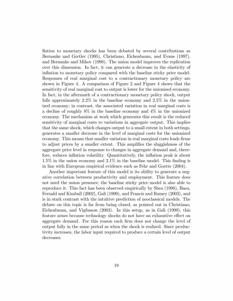
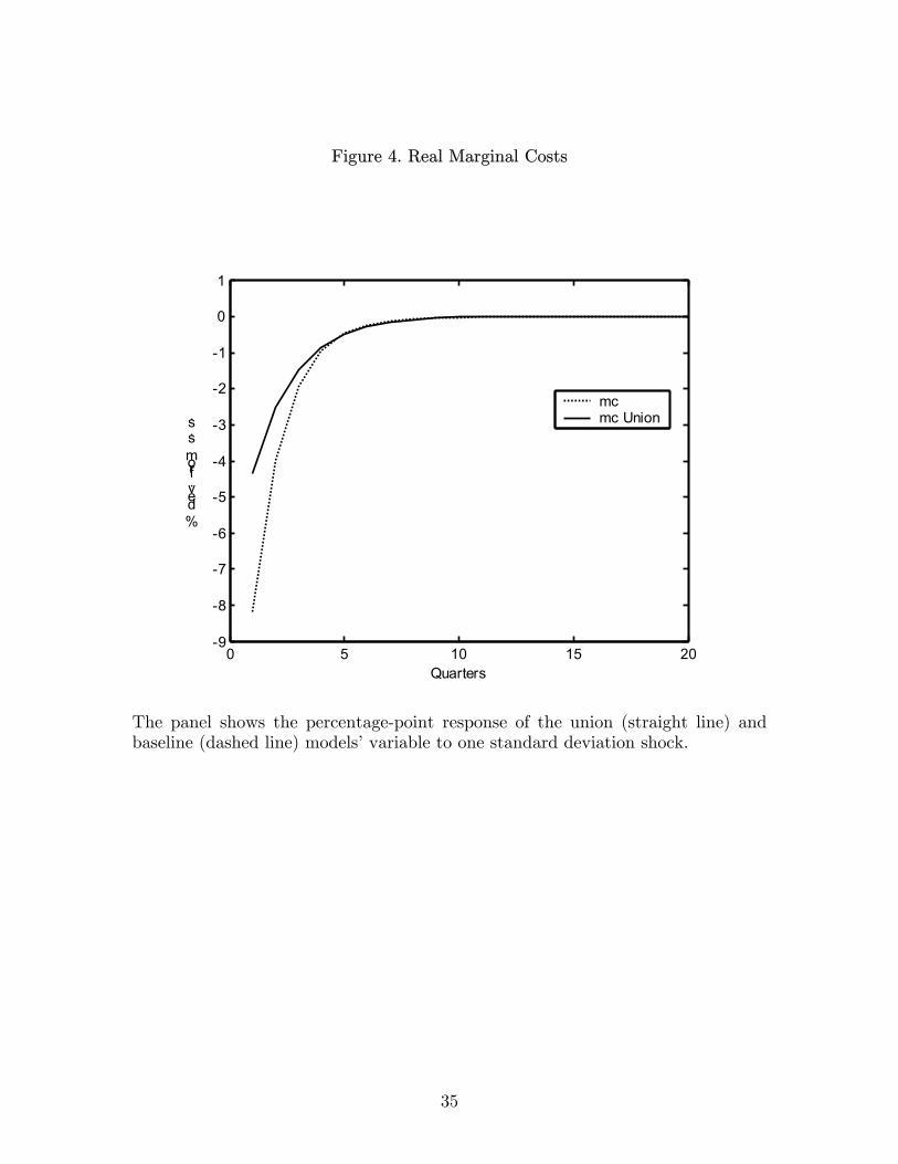
flation to monetary shocks has been debated by several contributions asBernanke and Gertler (1995), Christiano, Eichenbaum, and Evans (1997),and Bernanke and Mihov (1998). The union model improves the replicationover this dimension. In fact, it can generate a decrease in the elasticity ofinflation to monetary policy compared with the baseline sticky price model.Responses of real marginal cost to a contractionary monetary policy areshown in Figure 4. A comparison of Figure 2 and Figure 4 shows that thesensitivity of real marginal cost to output is lower for the unionized economy.In fact, in the aftermath of a contractionary monetary policy shock, outputfalls approximately 2.2% in the baseline economy and 2.5% in the union-ized economy; in contrast, the associated variation in real marginal costs isa decline of roughly 8% in the baseline economy and 4% in the unionizedeconomy. The mechanism at work which generates this result is the reducedsensitivity of marginal costs to variations in aggregate output. This impliesthat the same shock, which changes output to a small extent in both settings,generates a smaller decrease in the level of marginal costs for the unionizedeconomy. This means that smaller variation in real marginal costs leads firmsto adjust prices by a smaller extent. This amplifies the sluggishness of theaggregate price level in response to changes in aggregate demand and, there-fore, reduces inflation volatility. Quantitatively, the inflation peak is about1.5% in the union economy and 2.1% in the baseline model. This finding isin line with European empirical evidence such as Fehr and Goette (2004).Another important feature of this model is its ability to generate a neg-

ative correlation between productivity and employment. This feature doesnot need the union presence; the baseline sticky price model is also able toreproduce it. This fact has been observed empirically by Shea (1998), Basu,Fernald and Kimball (2002), Galì (1999), and Francis and Ramey (2003), andis in stark contrast with the intuitive prediction of neoclassical models. Thedebate on this topic is far from being closed, as pointed out in Christiano,Eichenbaum, and Vigfusson (2003). In this setup, as in Galì (1999), thisfeature arises because technology shocks do not have an exhaustive effect onaggregate demand. For this reason each firm does not change the level ofoutput fully in the same period as when the shock is realized. Since produc-tivity increases, the labor input required to produce a certain level of outputdecreases.

19

4.2 Model Simulations

The series for the variables are taken from Fagan, Henry, and Mestre (2001)and they are drawn from the European Central Bank data base. The dataare quarterly from 1980:1 through 1998:4. Output is measured by real GDP,consumption is measured by private consumption, investment is measuredby gross investment, employment is measured by standard units of labor,inflation is measured by changes in the GDP deflator, and the interest rateis measured by the short term interest rate. All data, except for the interestrate, are seasonally adjusted. The real variables are expressed in per-capitaterms by dividing by the total population between ages of 15 and 64. Allvariables, except inflation and the interest rate, are transformed into loga-rithms. All the series are H-P filtered so that only the cyclical componentremains.The state space representation of the model is used to generate realization

of the model by simulating a system of difference equations in st and ft forT periods by generating a (T ×1) dimensional series of Gaussian white noiseinnovations, εt, where T is the number of simulated periods that equals thenumber of periods in the observed time series of the economy. The simulatedstatistics are based on a set of 1000 simulations over a 76-quarter horizon, asthe size of the sample considered.Tables 2 through 4 list business cycle statistics for the Euro area macro-

economic variables output, consumption, investment, employment, inflation,and interest rates and compare them with the simulated series for the union(U) and baseline sticky price (SP) models. The statistics reproduced are thestandard deviation, the relative volatility (the ratio of the standard deviationof each variable and the standard deviation of output), and the correlationcoefficient with output.Table 2 shows the standard deviations for the variables under investi-

gation. A comparison of the union and the baseline models shows that thepresence of a representative union produces higher volatility for the real vari-ables, and lower volatility for inflation. The union model is better able toreplicate the variance of inflation, the interest rate, output, and consump-tion. The union model underperforms in the replication of the variance ofinvestment and employment.Table 3 compares the relative standard deviation of the variables with

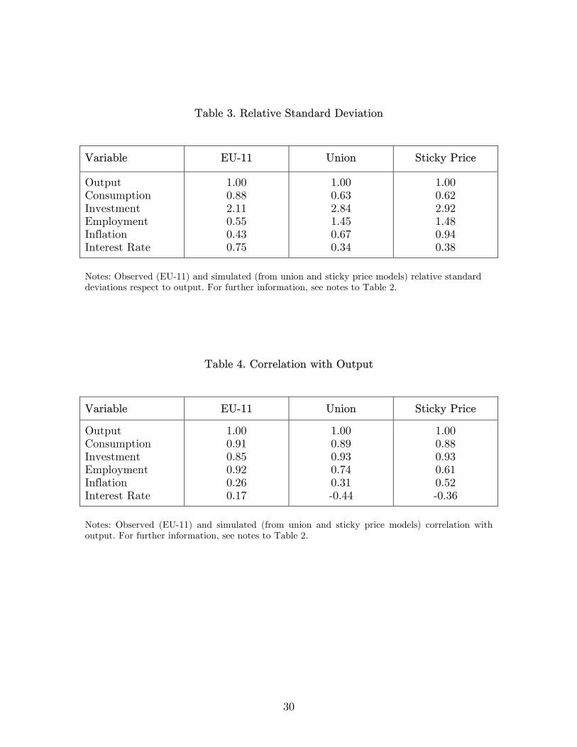
respect to output so that these statistics can be interpreted as the volatilityof the variables. From model’s simulations we notice that in the union model

20

the volatility of the nominal variables is lower and the volatility of the realvariables is higher, except for consumption. A comparison with the datashows that the union model matches the European economy better over all.The only mismatch is given by the interest rate for which the actual economystatistic is 0.75, whereas the union and baseline models produce values of 0.34and 0.38. Nonetheless, it must be noticed that the difference for this variablein the simulated models is small.Table 4 presents the correlations of the variables with output. As for the

previous measure, the volatility of the correlations is lower for the nominalvariables although the reverse relation does not hold for all the real variables.A shortcoming of both models is their inability to replicate the correlationof the interest rate with output. As Boivin and Giannoni (2003) point out,this may be due to the time span considered for the monetary policy rule.Nonetheless, the union model generates statistics closer to the ones in theactual economy.As a further exercise, I explore whether the model simulations produce

more persistence in the variables for the union model, as the theoreticalanalysis suggest. As inMaffezzoli (2001), I compare the correlations of supplyand demand shocks with lags and leads of the simulated series for bothunion and baseline models. Tables 5 and 6 reproduce these statistics for theproductivity and policy shocks respectively. For both shocks, the correlationin lead periods is higher in the union model, which suggests that the non-Walrasian setting delivers a higher degree of persistence.The overall lesson from these results is that the union model is better

able than the standard sticky price model to replicate several key aspects ofthe European business cycle.

5 Conclusions

This paper combines equilibrium unemployment generated through a simpleunion bargaining process into an otherwise standard New Keynesian mone-tary model. The combination of a non-Walrasian labor market with generalequilibrium models has been recently introduced in the New Keynesian liter-ature through efficiency wage and search models, and has been used to studybusiness cycles’ dynamics and shocks’ propagation. This paper is the firstattempt to introduce a union bargaining process to study interactions be-tween both supply and demand shocks and the business cycle in a monetary

21

sticky price model.The introduction of union bargaining produces two main results. First,

variables’ persistence in the aftermath of supply and demand shocks in-creases. The presence of the representative union in the economy generatesreal rigidities because of the lower wage volatility relative to a perfect compet-itive labor market. This feature produces an endogenous mechanism whichincreases variables’ persistence. Second, inflation becomes less volatile. Thesensitivity of real marginal costs to output is lower in the unionized economyso that firms adjust prices by a smaller extent compared to the competitivelabor market. The model is also able to reproduce the negative correlationbetween productivity shocks and employment that is observed in the data.Model simulations show the union model is superior to the standard stickyprice model in replicating European business cycles.

22

References

[1] Alexopoulos, M., (2002), Unemployment in a Monetary Business CycleModel, Unpublished manuscript, University of Toronto.

[2] Alexopoulos, M., (2004), Unemployment and the Business Cycle, Jour-nal of Monetary Economics, 51, 277-298.

[3] Barro, R., and Sala-i-Martin, X., (1999), Economic Growth, MIT Press.

[4] Basu, S., Fernald, J., and Kimball, M., (2002), Are Technology Im-provements Contractionary?, Harvard Institute of Economic Research,no. 1986.

[5] Bernanke, B., and Gertler, M., (1995), Inside the Black Box: The CreditChannel of Monetary Policy Transmission, Journal of Economic Per-spectives, Vol. 9, no. 4, 24-48.

[6] Bernanke, B., and Mihov, I., (1998), Measuring Monetary Policy, Quar-terly Journal of Economics, Vol. 113, no. 3, 869-902.

[7] Blanchard, O., and Khan, C., (1980), The Solution of Linear DifferenceModels under Rational Expectation, Econometrica, 48, no. 5, 1305-1311.

[8] Boivin, J., Giannoni, M., (2003), Has Monetary Economics Becomemore Effective?, NBER Working Paper Series, No. 9459.

[9] Carlstrom, C., and Fuerst, T., (2000), Forward vs. Backward-LookingTaylor Rules, Working Paper, Federal Reserve Bank of Cleveland.

[10] Chari, V., V., Kehoe, P., J., and McGrattan, E., (2000), Sticky PriceModels of the Business Cycle: Can the Contract Multiplier Solve thePersistence Problem, Econometrica, Vol. 68, 1151-1579.

[11] Christiano, L., and Eichenbaum, M., (1992), Current Real Business Cy-cle Theories and Aggregate Labor Market Fluctuations, American Eco-nomic Review, Vol. 82, no. 3, 430-450.

[12] Christiano, L., Eichenbaum, M., and Evans, C., (1997), Sticky Pricesand Limited Participation Models: A Comparison, European EconomicReview, 41, 1201-1249.

23

[13] Christiano, L., Eichenbaum, M., and Evans, C., (2004), Nominal Rigidi-ties and the Dynamic Effects of a Shock to Monetary Policy, Journal ofPolitical Economy, forthcoming.

[14] Christiano, L., Eichenbaum, M., and Vigfusson, R., (2003), What Hap-pens After a Technology Shock, Board of Governors of the Federal Re-serve System Discussion Paper, No. 768.

[15] Clarida, R., Galì, J., and Gertler, M., (1998), Monetary Policy Rules inPractice: some International Evidence, European Economic Review, 42,1033-1067.

[16] Daveri, F., and Maffezzoli, M., (2000), A Numerical Approach to Fis-cal Policy, Unemployment and Growth in Europe, Bocconi University-IGIER Working Paper.

[17] Dotsey, M., and King, R., (2001), Pricing, Production and Persistence,NBER Working Paper Series, No. 8407.

[18] Fagan, G., Henry, J., and Mestre, R., (2001), An Area Wide Model(AWM) for the Euro Area, ECB Working Paper Series, No. 42.

[19] Farber, H.S., (1986), The Analysis of Union Behaviour, in Ashenfelter,Layard (Eds.), Handbook of Labor Economics, North Holland, Amster-dam, Vol. II.

[20] Fehr, E. and Goette, L., 2004, Robustness and Real Consequences ofNominal Wage Rigidity, Journal of Monetary Economics, forthcoming.

[21] Francis, N., and Ramey, V., (2003), Is the Technology Driven Real Busi-ness Cycle Hypothesis Dead? Shocks and Aggregate Fluctuations Re-vised, Unpublished Manuscript, University of California at San Diego.

[22] Galì, J., (1999), Technology, Employment, and the Business Cycle: DoTechnology Shocks Explain Aggregate Fluctuations?, American Eco-nomic Review, Vol. 89, no. 1, 249-271.

[23] Galì, J., Gertler, M., and Lopez-Salido, D., (2002), Markups, gaps andWelfare Costs of Business Fluctuations, NBER Working Paper Series,No. 8850.

24

[24] Hall, R., (2000), Labor Market Frictions and Unemployment Fluctu-ations, Handbook of Macroeconomics, (Woodford, M., and Taylor, J.,Eds.), Vol. IB. Amsterdam/New York, Elsevier.

[25] Ireland, P., (2000), Interest Rates, Inflation, and Federal Reserve PolicySince 1980, Journal of Money Credit and Banking, 32, 417-434.

[26] Kimball, M., (1995), The Quantitative Analytics of the Basic Neomon-etarist Model, Journal of Money, Credit, and Banking, 27, 1241-1277.

[27] King, R., and Rebelo, S., (2000), Resuscitating Real Business Cycle,Handbook of Macroeconomics, (Woodford, M., and Taylor, J., Eds.),Vol. IB. Amsterdam/New York, Elsevier.

[28] Klein, P., (2000), Using the Generalized Schur Form to Solve a Multi-variate Linear Rational Expectations Model, Journal of Economic Dy-namics & Control, 24, 1405-1423.

[29] Maffezzoli, M., (2001), Non-Walrasian Labor Markets and Real BusinessCycle, Review of Economics Dynamics, 4, 860-892.

[30] Manning, A., (1987), An Integration of Trade Union Model in a Sequen-tial Bargaining Framework, Economic Journal, 97, 121-139.

[31] Mortersen, D., and Pissarides, C., (1994), Job Creation and Job Destruc-tion in the Theory of Unemployment, Review of Economics Studies, 61,397-415.

[32] Nickell, S., (1982), A Bargaining Model of the Phillips Curve, Centerfor Labor Economics Discussion Paper, Nr. 130.

[33] OECD (1997), Employment Outlook.

[34] OECD (2002), Economic Outlook.

[35] Pencavel, J., (1986), Labor Supply of Men: a Survey, in Ashenfelter andLayard (Eds.), Handbook of Labor Economics, North Holland, Amster-dam, 3-102.

[36] Pissarides, C., (1990), Equilibrium Unemployment Theory, The MITPress.

25

[37] Pissarides, C., (1998), The Impact of Employment Tax Cut on Un-employment and wages; The Role of Unemployment Benefits and TaxStructure, European Economic Review, 42, 155-183.

[38] Rogerson, R., and Wright, R., (1988), Involuntary Unemployment inEconomics with Efficient Risk Sharing, Journal of Monetary Economics,22, 501-515.

[39] Rotemberg, J., and Woodford, M., (1992), Oligopolistic Pricing and theEffects of aggregate Demand on Economic Activity, Journal of PoliticalEconomy, 100, 1153-1207.

[40] Shea, J., (1998), What do Technology Shocks Do?, NBER Macroeco-nomics Annual.

[41] Smets, F., and Wouters, R., (2003), An estimated Stochastic DynamicsGeneral Equilibrium Model of the Euro Area, Journal of the EuropeanEconomic Association, 5, 1123-1175.

[42] Taylor, J., (1999), Monetary Policy Rules, (Eds.), NBER Business CycleSeries, Vol. 31.

[43] Trigari, A., (2004), Equilibrium Unemployment, Job Flows and InflationDynamics, ECB Working Paper Series, No. 304.

[44] Walsh, C., (2003), Labor Market Search, Sticky Prices and Interest RateRules, University of Santa Clara Working Paper Series.

[45] Woodford, M., (2001), The Taylor Rule and Optimal Monetary Policy,American Economic Review, 2001, 91(2), 232-237.

26

6 Appendix

This Appendix shows how to derive the representative household’s utilityfunction as it appears in equation (1). King, Plosser, and Rebelo (1988)show that a utility function in consumption and leisure can be expressed as

Ut =1

1− µ [Ctv(nt)]1−µ − 1, (A.1)

where the function v(nt) satisfies at some regularity conditions.4 The mar-ginal utility of consumption of (A.1) can be expressed as

U1(Ct, nt,Mt

Pt) = C−µt v(nt)

1−µ.

Assuming perfect risk sharing, the marginal utility of consumption foremployed (e) and unemployed (u) members of the household is the same.Therefore, the following holds

C−µet ve(nt)1−µ = C−µut vu(nt)

1−µ (A.2)

The average consumption for the representative household can be writtenas

Ct = ntCet + (1− nt)Cut. (A.3)

Using equation (A.2), expression (A.3) can be written as

Cet =Ct

nt + (1− nt)vu(nt)ve(nt)

. (A.4)

The utility for the representative household can be written as

ntU(Cet, nt,Mt

Pt) + (1− nt)U(Cut, 1− nt, Mt

Pt) (A.5)

= [Cetve(nt)]1−µ

½nt + (1− nt)

·Cutvu(nt)

Cetve(nt)

¸¾+ κm

Mt

Pt.

4Namely, from King, Plosser, and Rebelo (1988), v(n) is twice continuously differen-tiable and, since µ > 1, v(n) is decreasing and convex. In addition, to assure the overallconcavity of U , −µv(n)vnn(n) > (1− 2µ) [vn(n)]2.

27

Equations (A.2) and (A.4) into (A.5) yield

U(Ct, nt,Mt

Pt) = ve(nt)

1−µC1−µt

(nt + (1− nt)

·Cutvu(nt)

Cetve(nt)

¸ 1−µµ

)µ+ κm

Mt

Pt

which is equivalent to equation (1) in the paper once the irrelevant termve(nt)

1−µ is dropped and the function is rescaled for the constant -1.

28

29

Table 1. Union Density and Bargaining Coverage Rates

Country

Union Density

Bargaining Coverage

1980

1990

1994

1980

1990

1994

United States

22

16

16

26

18

18

Euro Area

49.7

42.9

44.3

82.6

81.3

82.3

Source: OECD, Employment Outlook (1997) and computations from the author.

Table 2. Standard Deviation

Variable

EU-11

Union

Sticky Price

Output Consumption Investment Employment Inflation Interest Rate

1.31 1.15 2.76 1.16 0.56 0.98

1.28 0.80 3.61 1.84 0.84 0.43

1.05 0.65 3.06 1.53 0.97 0.40

Notes: Observed (EU-11) and simulated (from union and sticky price models) standard deviations. The observed statistics are based on seasonally adjusted quarterly data from Fagan, Henry, and Mestre (2001) from 1980:1 to 1998:4. The real variables are expressed in per-capita terms by dividing by the total population, age between 15 and 64. Variables, except inflation, and interest rate, are transformed in logarithms. All the series are H-P filtered so that only the cyclical component remains. The simulated business cycle statistics are based on 1000 simulations over 76 quarter horizon and are H-P filtered for comparison purposes. Simulated figures are averages across simulations.

30

Table 3. Relative Standard Deviation

Variable

EU-11

Union

Sticky Price

Output Consumption Investment Employment Inflation Interest Rate

1.00 0.88 2.11 0.55 0.43 0.75

1.00 0.63 2.84 1.45 0.67 0.34

1.00 0.62 2.92 1.48 0.94 0.38

Notes: Observed (EU-11) and simulated (from union and sticky price models) relative standard deviations respect to output. For further information, see notes to Table 2.

Table 4. Correlation with Output

Variable

EU-11

Union

Sticky Price

Output Consumption Investment Employment Inflation Interest Rate

1.00 0.91 0.85 0.92 0.26 0.17

1.00 0.89 0.93 0.74 0.31 -0.44

1.00 0.88 0.93 0.61 0.52 -0.36

Notes: Observed (EU-11) and simulated (from union and sticky price models) correlation with output. For further information, see notes to Table 2.

31

Table 5. Correlations of Simulated Series with Supply Shocks

Output

Consumption

Investment

Employment

Inflation

Inter.Rate

U

SP

U

SP

U

SP

U

SP

U

SP

U

SP t+3

t+2

t+1

t

t-1

t-2

t-3

0.30

0.42

0.53

0.54

0.29

0.10

-0.02

0.23

0.37

0.50

0.56

0.32

0.14

0.02

0.26

0.44

0.65

0.85

0.48

0.21

0.02

0.22

0.41

0.64

0.88

0.52

0.26

0.07

0.28

0.34

0.34

0.20

0.08

0.00

-0.06

0.20

0.28

0.31

0.22

0.11

0.03

-0.03

0.24

0.22

0.12

-0.16

-0.15

-0.13

-0.12

0.13

0.09

-0.02

-0.30

-0.22

-0.15

-0.10

0.11

0.00

-0.22

-0.62

-0.41

-0.25

-0.13

0.10

0.04

-0.09

-0.40

-0.28

-0.18

-0.10

-0.33

-0.32

-0.16

-0.06

0.02

0.07

0.10

-0.26

-0.28

-0.16

-0.07

0.00

0.04

0.06

Notes: Correlations of different leads and lags of simulated series from union (U) and sticky price (SP) models with supply shocks. All series have been H-P filtered; all figures are averaged across simulations.

Table 6. Correlations of Simulated Series with Demand Shocks

Output

Consumption

Investment

Employment

Inflation

Inter.Rate

U

SP

U

SP

U

SP

U

SP

U

SP

U

SP t+3

t+2

t+1

t

t-1

t-2

t-3

-0.03

-0.13

-0.30

-0.62

0.16

0.14

0.12

0.01

-0.07

-0.27

-0.68

0.13

0.12

0.10

-0.03

-0.09

-0.18

-0.35

0.13

0.10

0.08

-0.01

-0.05

-0.15

-0.37

0.09

0.08

0.06

-0.02

-0.14

-0.36

-0.75

0.17

0.15

0.13

0.02

-0.08

-0.31

-0.82

0.15

0.13

0.11

-0.03

-0.15

-0.36

-0.75

0.18

0.15

0.14

0.02

-0.08

-0.31

-0.81

0.14

0.12

0.10

-0.01

-0.11

-0.29

-0.62

0.12

0.10

0.10

0.02

-0.07

-0.30

-0.78

0.13

0.11

0.10

0.15

0.36

0.74

-0.18

-0.15

-0.13

-0.11

0.08

0.32

0.83

-0.15

-0.13

-0.11

-0.10

Notes: Correlations of different leads and lags of simulated series from union (U) and sticky price (SP) models with demand shocks. All series have been H-P filtered; all figures are averaged across simulations.

32

Figure 1. Unemployment Rates in the Euro Area and the United States

0

2

4

6

8

10

12

1980

1981

1982

1983

1984

1985

1986

1987

1988

1989

1990

1991

1992

1993

1994

1995

1996

1997

1998

1999

2000

2001

2002

United States

Euro Area

The panel shows unemployment rate for the euro area (straight line) and the United States (dashed line). Source: OECD, Outlook (2002).

33

Figure 2. Impulse Response Functions to a Monetary Policy Shock

0 5 10 15 20-1

-0.5

0

Quarters

% dev. from s. s.

c c Union

0 5 10 15 20-6

-4

-2

0

nn Union

0 5 10 15 200

2

4

6λλ Union

0 5 10 15 20-10

-5

0

ii Union

0 5 10 15 20-0.03

-0.02

-0.01

0

γγ Union

0 5 10 15 20-15

-10

-5

0

5

qq Union

0 5 10 15 20-3

-2

-1

0

yy Union

0 5 10 15 20-6

-4

-2

0

2

ww Union

0 5 10 15 20-4

-2

0

2

ξξ Union

0 5 10 15 20-3

-2

-1

0

1

ππ Union

0 5 10 15 20-0.4

-0.3

-0.2

-0.1

0

kk Union

0 5 10 15 200

0.5

1rr Union

0 5 10 15 20-5

0

5

10

15ff Union

Each panel shows the percentage-point response of the union (straight line) and baseline (dashed line) models’ variables to one standard deviation monetary policy shock.

34

Figure 3. Impulse Response Functions to a Productivity Shock

0 5 10 15 200

0.2

0.4

0.6

0.8

Quarters

% dev. from s. s. c

c Union

0 5 10 15 20-1

-0.5

0

0.5

nn Union

0 5 10 15 20-2

-1.5

-1

-0.5

0

λλ Union

0 5 10 15 200

0.5

1

1.5

2ii Union

0 5 10 15 20-5

0

5x 10

-3

γγ Union

0 5 10 15 20-2

-1

0

1

qq Union

0 5 10 15 200

0.5

1yy Union

0 5 10 15 20-0.5

0

0.5

ww Union

0 5 10 15 20-3

-2

-1

0

ξξ Union

0 5 10 15 20-0.8

-0.6

-0.4

-0.2

0

ππ Union

0 5 10 15 200

0.1

0.2

0.3

0.4kk Union

0 5 10 15 20-0.2

-0.1

0

0.1

0.2rr Union

0 5 10 15 200

1

2

3

4ff Union

Each panel shows the percentage-point response of the union (straight line) and baseline (dashed line) models’ variables to one standard deviation productivity shock.

35

Figure 4. Real Marginal Costs

0 5 10 15 20-9

-8

-7

-6

-5

-4

-3

-2

-1

0

1

Quarters

% dev. from s. s.

mc mc Union

The panel shows the percentage-point response of the union (straight line) and baseline (dashed line) models’ variable to one standard deviation shock.