Embed Size (px)
Citation preview
HAL Id: inria-00392881https://hal.inria.fr/inria-00392881
Submitted on 9 Jun 2009
HAL is a multi-disciplinary open accessarchive for the deposit and dissemination of sci-entific research documents, whether they are pub-lished or not. The documents may come fromteaching and research institutions in France orabroad, or from public or private research centers.
L’archive ouverte pluridisciplinaire HAL, estdestinée au dépôt et à la diffusion de documentsscientifiques de niveau recherche, publiés ou non,émanant des établissements d’enseignement et derecherche français ou étrangers, des laboratoirespublics ou privés.
Combinative preconditioning based on Relaxed NestedFactorization and Tangential Filtering preconditioner
Pawan Kumar, Laura Grigori, Frédéric Nataf, Qiang Niu
To cite this version:Pawan Kumar, Laura Grigori, Frédéric Nataf, Qiang Niu. Combinative preconditioning based onRelaxed Nested Factorization and Tangential Filtering preconditioner. [Research Report] RR-6955,INRIA. 2009. inria-00392881

appor t de r ech er ch e
ISS
N02
49-6
399
ISR
NIN
RIA
/RR
--69
55--
FR
+E
NG
Thème NUM
INSTITUT NATIONAL DE RECHERCHE EN INFORMATIQUE ET EN AUTOMATIQUE
Combinative preconditioning based on RelaxedNested Factorization and Tangential Filtering
preconditioner
Pawan Kumar — Laura Grigori — Frederic Nataf — Qiang Niu
N° 6955
Juin 2009


Centre de recherche INRIA Saclay – Île-de-FranceParc Orsay Université
4, rue Jacques Monod, 91893 ORSAY CedexTéléphone : +33 1 72 92 59 00
Combinative pre onditioning based on RelaxedNested Fa torization and Tangential Filteringpre onditionerPawan Kumar∗ , Laura Grigori† , Frederi Nataf‡ , Qiang Niu§Thème NUM Systèmes numériquesÉquipe-Projet Grand-largeRapport de re her he n° 6955 Juin 2009 24 pagesAbstra t: The problem of solving blo k tridiagonal linear systems arising fromthe dis retization of PDE is onsidered. The nested fa torization pre onditionerintrodu ed by [J. R. Appleyard and I. M. Cheshire, Nested Fa torization, SPE12264, presented at the Seventh SPE Symposium on Reservoir Simulation, SanFran is o, 1983 is an ee tive pre onditioner for ertain lass of problems and asimilar method is implemented in S hlumerger's E lipse oil reservoir simulator.In this paper, a relaxed version of Nested Fa torization pre onditioner isproposed as a repla ement to ILU(0). Indeed, the proposed pre onditioner isSPD and leads to a stable splitting if the input matrix is S.P.D. . For ILU(0),equivalent properties hold if the input matrix is a M-matrix. Moreover it hasno storage ost. Ee tive multipli ative/additive pre onditioning is a hievedin ombination with Tangential ltering pre onditioner with the lter ve tor hosen as ve tor of ones. Numeri al tests are arried out with both additiveand multipli ative ombinations. With this setup the new pre onditioner is asrobust as the ombination of ILU(0) with tangential ltering pre onditioner.Key-words: pre onditioner, linear system, frequen y ltering de omposition,GMRES, nested fa torization, in omplete LU, eigenvalues∗ INRIA Sa lay - Ile de Fran e, Laboratoire de Re her he en Informatique, UniversiteParis-Sud 11, Fran e (Email:pawan.kumarlri.fr)† INRIA Sa lay - Ile de Fran e, Laboratoire de Re her he en Informatique, UniversiteParis-Sud 11, Fran e (Email:laura.grigoriinria.fr)‡ Laboratoire J. L. Lions, CNRS UMR7598, Universite Paris 6, Fran e; Email:natafann.jussieu.fr§ S hool of Mathemati al S ien es, Xiamen University, Xiamen, 361005, P.R. China; Thework of this author was performed during his visit to INRIA, funded by China S holarshipCoun il; Email:kangniugmail. om

Pré onditionnement basé sur fa torisationemboîtée et ltrage tangentielRésumé : Dans e papier nous présentons une version de fa torisation em-boîté ave relaxation. Cette fa torisation est proposée omme rempla ement deILU(0). Le pré onditionneur proposé est SPD si la matri e originale est SPD.Pour ILU(0)des propriété équivalentes existent si la matri e originale est uneM-matri e. Un pré onditionnement e a e est obtenu en ombinaison ave leltrage tangentiel ave le ve teur de ltrage de ones. Des tests numériques sontprésentés pour des ombinaisons additifs et multipli atifs. Ils montrent que lepré onditionneur est aussi robuste que la ombinaison obtenue par ILU(0)ave le ltrage tangentiel.Mots- lés : pré onditionnement, fa torisation emboîtée, fa torisation LUin omplète

Combinative pre onditioning based on RNF and Tangential Filtering 31 INTRODUCTIONSeveral appli ations are modelled by non-linear partial dierential equations,examples in lude oil reservoir simulations and uid ow through porous me-dia. These equations are usually solved by the Newton's method or xed pointmethod, where at ea h step a pre onditioned iterative method is generally usedfor solving a large sparse linear systemAx = b. (1)The linear systems hange at ea h step, and solving them onstitute the most omputationally intensive part of the simulation. Therefore, an e ient pre on-ditioner with fast setup time plays an important role in the overall simulationpro ess. Also, sin e the systems are very large, the pre onditioner should notbe too demanding in terms of memory requirements. This problem has al-ready been extensively studied, see [7, 16, 18 for the des ription of algorithmsand their omparisons. In parti ular, one lass of methods whi h have provedparti ularly su essful are the algebrai multigrid methods, see for example,[17, 19, 20, 24. However, for ertain problems the algebrai multigrid meth-ods involve relatively high setup ost, whi h leads us to look into some otheralternatives in this work.With fast setup time and very modest storage requirement, the Nested Fa -torization (NF) pre onditioner introdu ed in [1 is a powerful pre onditioner;it has been found [1, 15 that for ertain lass of problems it performs betterthan the widely used ILU(0) or Modied ILU [18. NF takes as input a matrixwhi h has a nested blo k tridiagonal stru ture. Matri es arising from the dis- retization of P.D.E an be permuted to this form. The method of NF diersfrom ILU(0) or Modied ILU(0) in that the pre onditioning matrix in NF is notformed stri tly from upper and lower triangular fa tors. Instead, blo k lowerand upper fa tors are onstru ted using a pro edure whi h adds one dimensionat a time to the pre onditioning matrix having the diagonal matrix on the lowestlevel.The NF pre onditioner has some important properties. If BNF is the NF pre- onditioner, then colsum(BNF −A) = 0 (also known as zero olsum property),as a onsequen e the sum of the residuals in su essive Krylov iterations remainzero, provided a suitable initial solution is used [1. This property an provide avery useful he k on the orre tness of the implementation. Further, quoting [1,the fa torization pro edure onserves material exa tly for ea h phase at ea hlinear iteration, and a ommodates non-neighbour onne tions (arising from thetreatment of the faults, ompleting the ir le in three-dimensional oning stud-ies, numeri al aquifers, dual porosity/permeability systems et .) in a naturalway. Moreover, for uid ow problems it is proved in [2 that the lower and theupper triangular fa tors of NF are nonsingular. Due to these desirable qualities,the NF pre onditioner is of parti ular interest in the oil reservoir industry; amethod similar to NF is implemented in S hlumerger's E lipse oil reservoir sim-ulator [12. However, as we will see later in the tables, the NF pre onditioner an fail on some problems.The main result of this paper is the introdu tion of a new pre onditionerwhi h orresponds to a relaxed version of NF, namely RNF(0,0). Compared toILU(0), it has several important properties:RR n° 6955

4 Pawan Kumar , Laura Grigori , Frederi Nataf , Qiang Niu If A is S.P.D. then,RNF(0,0) is S.P.D.RNF(0,0) leads to a stable splitting no setup ost no storage requirementThe new pre onditioner is parti ularly useful when multipli ate/additive pre- onditioning is a hieved in ombination with tangential ltering pre onditioner[4. With this setup the new pre onditioner is as robust as the ombinationof ILU(0)with tangential ltering pre onditioner. Notably both multipli ativeand additive ombination are tried. Good results are obtained with the additive ombination whi h moreover has an advantage over multipli ative ombinationon parallel systems; ea h of the pre onditioner solves involved with the additive ase an be done simultaneously on two dierent pro essors. In order to makea omprehensive study, we onsider a general relaxed version of NF, namelyRNF(α,β).This arti le is organized as follows. Notations play an important role inexplaining the method of NF; we arefully introdu e them in the next se tion.In se tion 3, NF is explained and later in the se tion RNF is introdu ed. Themethod of LFTFD is dis ussed briey in se tion 4. In se tion 5, we present onvergen e results for the ombination involving RNF(0,0) and LFTFD whi hshows that the ombination is onvergent. In se tion 6 we will omment onnumeri al results. And nally, se tion 7 on ludes the paper.2 NOTATIONSThroughout the paper, matrix A is onsidered to be arising from the nitedieren e or nite volume dis retization of two or three dimensional partialdierential equations. For example, using 7-point formula for three dimensionalproblems for an nx×ny×nz grid, where nx denotes the number of points on theline, ny denotes the number of lines on ea h plane, and nz denotes the numberof planes, we obtain an (nx×ny×ny)× (nx×ny×nz) matrix. Let nxy denotenx× ny, the number of unknowns on ea h plane, nyz denote ny ×nz, the totalnumber of lines on all planes, and nxyz denote nx× ny × nz, the total numberof unknowns. Then the resulting matrix has a nested tridiagonal stru ture asfollows:
A =
D1 U13
L13 D2
. . .. . . . . . Unz−13
Lnz−13 Dnz
. (2)Here the diagonal blo ks Dis are the blo ks orresponding to the unknownsof the ith plane. The blo ks Li3 and U i
3 are diagonal matri es of size nxy, andthey orrespond to the onne tions between the ith and (i + 1)th plane. Fur-ther, the diagonal blo ks Dis are themselves blo k tridiagonal, i.e. they haveINRIA

Combinative pre onditioning based on RNF and Tangential Filtering 5the following stru ture,Di =
D(i−1)∗ny+1 U(i−1)∗ny+1
2
L(i−1)∗ny+1
2 D(i−1)∗ny+2
. . .. . . . . . Ui∗ny−1
2
Li∗ny−1
2 Di∗ny
where the blo ks L
i
2 and Ui
2 are diagonal matri es of size nx ea h and they orrespond to the onne tions between the lines. The diagonal blo ks Di arethemselves tridiagonal matri es,Di =
D(i−1)∗nx+1 U(i−1)∗nx+11
L(i−1)∗nx+11 D(i−1)∗nx+2
. . .. . . . . . Ui∗nx−1
Li∗nx−11 Di∗nx
with the s alars L
(i−1)∗nx+j1 and U
(i−1)∗nx+j1 being the orresponding onne -tions between the ells. We observe that this matrix has nested tridiagonalstru ture. For any matrix K, Diag(K) refers to the stri t diagonal of K; forany ve tor v, Diag(v) refers to the diagonal matrix formed from the ve tor v.For any diagonal matrix M of size nxyz, the ith entry of M is denoted by Mi,the ith line blo k of M is denoted by M i, and the ith plane blo k of M is denotedby Mi. Below we list the stru tures of the matri es L1, U1, L2, U2, L3, and U3to be referred to later.
RR n° 6955

6 Pawan Kumar , Laura Grigori , Frederi Nataf , Qiang NiuDiag(A) =
D1
D2 . . .Dnxyz
, M =
M1
M2 . . .Mnxyz
L1 =
0
L11 0. . . . . .
Lnxyz−11 0
, U1 =
0 U11
0. . .. . . U1
nxyz−1
0
L2 =
0
L1
2
. . .. . . . . .. . . . . .L
nyz−1
2 0
, U2 =
0 U1
2. . . . . .. . . . . .. . . Unyz−1
2
0
L3 =
0
L13
. . .. . . . . .. . . . . .Lnz−1
3 0
, U3 =
0 U13. . . . . .. . . . . .. . . Unz−1
3
0
3 RELAXED NESTED FACTORIZATIONIn this se tion, we introdu e RNF for three-dimensional ase, the two-dimensional ase will be onsidered a spe ial ase of three-dimensional ase with just oneplane. We rst introdu e a spe ial version of the pre onditioner for whi h weprove that it is S.P.D when the input matrix A is S.P.D . Later, we introdu e amore general version whi h will prove signi ant for the two-dimensional prob-lems.3.1 A spe ial ase : RNF(0,0)We dene the RNF(0,0) pre onditioner as follows:
BRNF (0,0) = (P + L3)(I + P−1U3)
P = (T + L2)(I + T−1U2)
T = (M + L1)(I + M−1U1)
M = diag(A) .3.2 The general ase : RNF(α,β)The general version of relaxed nested fa torization pre onditioner denoted byBRNF (α,β) is dened hierar hi ally as follows: INRIA
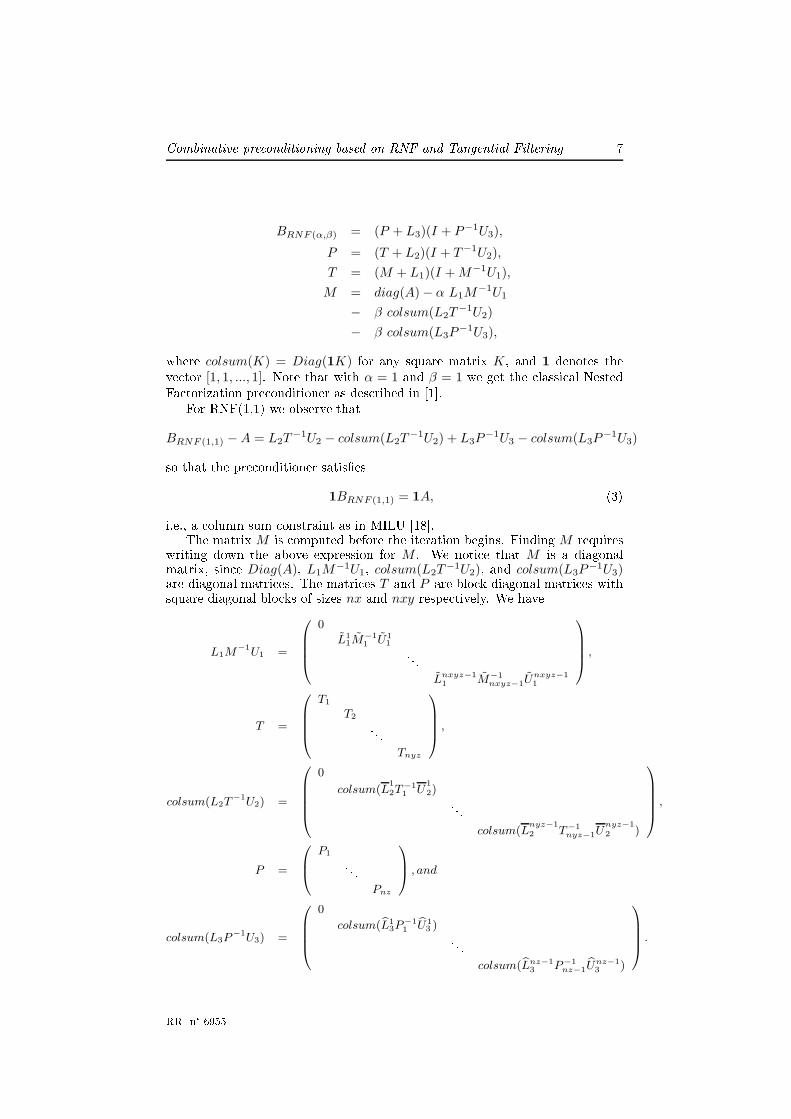
Combinative pre onditioning based on RNF and Tangential Filtering 7BRNF (α,β) = (P + L3)(I + P−1U3),
P = (T + L2)(I + T−1U2),
T = (M + L1)(I + M−1U1),
M = diag(A) − α L1M−1U1
− β colsum(L2T−1U2)
− β colsum(L3P−1U3),where colsum(K) = Diag(1K) for any square matrix K, and 1 denotes theve tor [1, 1, ..., 1]. Note that with α = 1 and β = 1 we get the lassi al NestedFa torization pre onditioner as des ribed in [1.For RNF(1,1) we observe that
BRNF (1,1) − A = L2T−1U2 − colsum(L2T
−1U2) + L3P−1U3 − colsum(L3P
−1U3)so that the pre onditioner satises1BRNF (1,1) = 1A, (3)i.e., a olumn sum onstraint as in MILU [18.The matrix M is omputed before the iteration begins. Finding M requireswriting down the above expression for M . We noti e that M is a diagonalmatrix, sin e Diag(A), L1M−1U1, colsum(L2T
−1U2), and colsum(L3P−1U3)are diagonal matri es. The matri es T and P are blo k diagonal matri es withsquare diagonal blo ks of sizes nx and nxy respe tively. We have
L1M−1
U1 =
0BBB@
0
L1
1M−1
1U1
1 . . .L
nxyz−1
1M−1
nxyz−1U
nxyz−1
1
1CCCA ,
T =
0BBB@
T1
T2 . . .Tnyz
1CCCA ,
colsum(L2T−1
U2) =
0BBBB@
0
colsum(L1
2T−1
1U
1
2) . . .colsum(L
nyz−1
2 T−1
nyz−1U
nyz−1
2 )
1CCCCA
,
P =
0B@
P1 . . .Pnz
1CA , and
colsum(L3P−1
U3) =
0BBB@
0
colsum(bL1
3P−1
1bU1
3 ) . . .colsum(bLnz−1
3P−1
nz−1bUnz−1
3)
1CCCA .
RR n° 6955

8 Pawan Kumar , Laura Grigori , Frederi Nataf , Qiang Niu3.3 Constru tion of RNF(α, β) pre onditionerA detailed pseudo ode for the onstru tion of RNF (α, β) pre onditioner is pro-vided in Algorithm (1), we briey outline the onstru tion in this se tion. Theentries of M are al ulated in a single sweep through the grid. Reading theentries row by row for the expression of M , we an determine M .The rst row gives M1 = D1. For the se ond ell onwards up to the last ellof rst line there are ontributions from the term L1M−1U1, and we have
Mi = Di − Li−11 U i−1
1 /Mi−1, i = 2, . . . , nx.When the update from the rst line is nished, ea h element of M for the se ondline also depends on the previous line through the term colsum(L2T−1U2), andea h element of M for se ond plane onwards depends on the previous planethrough the term colsum(L3P
−1U3). The (j + 1)th line blo k of the blo kdiagonal matrix colsum(L2T−1U2), an be omputed as follows:
colsum(Lj
2T−1j U
j
2) = Diag(1Lj
2T−1j U
j
2) = Diag((Uj
2)T T−T
j (Lj
2)T1).A similar al ulation an be performed for the omputation of the plane blo ksof colsum(L3P
−1U3).3.4 Solution pro edureIn this se tion we will see how the nested expression for B is used to solve theequationBRNF (α,β)u = vrequired in a pre onditioned Krylov iterative method. At the outermost level,we solve
(P + L3)(I + P−1U3)u = vdoing the forward sweeps of the form q = P−1i (v − Li−1
3 q), and the ba kwardsweeps of the form u = u − P−1i U i
3q. These equations are solved for one planeat a time. The solution involves solving equations of the form Piw = x forea h plane. To solve this equation we use the fa t that ea h plane blo k of thepre onditioner has an in omplete blo k fa torization represented byP = (T + L2)(I + T−1U2),and we solve Piw = x using the forward sweeps of the form r = T−1
i (x−Li−1
2 r),and the ba kward sweeps of the form w = w−T−1i U
i
2r. We noti e that we needto solve equations of the form Tiy = z orresponding to ea h line blo k of thepre onditioner, and for this we use the following fa tored form of T
T = (M + L1)(I + M−1U1),and we solve Tiy = z using the forward sweeps of the form s = M−1i (z− Li−1
1 s),and the ba kward sweeps of the form y = y − M−1i U i
1s. INRIA

Combinative pre onditioning based on RNF and Tangential Filtering 9
Algorithm 1 PSEUDOCODE TO FIND M FOR RNF(α, β)INPUT: Diag(A), L1, L2, L3, U1, U2, U3OUTPUT: Mfor i = 1 to nz (Number of planes) doif i 6= 1 and β 6= 0 (Not the rst plane) thenSolve PTi−1x = (L3
i−1)T .1
Mi = Mi - β(U3
i−1)T xend ifUPDATE-FROM-LINES(Mi)end forUPDATE-FROM-LINES(Mi)for j = 1 to ny (Number of lines in urrent plane) doif j 6= 1 and β 6= 0(Not the rst line) thenSolve T T
j−1x = (L2j−1
)T .1
M (i−1)∗ny+j = M (i−1)∗ny+j - β(Uj−1
2 )T xend ifUPDATE-FROM-CELLS(M (i−1)∗ny+j)end forUPDATE-FROM-CELLS(M i)M(i−1)∗nx+1 = D(i−1)∗nx+1 (Update from rst ell of urrent line)for k = 2 to nx (Update from rest of the ells) do
M(i−1)∗nx+k = M(i−1)∗nx+k - α L(i−1)∗nx+k−11 M−1
(i−1)∗nx+k−1U(i−1)∗nx+k−11end for
RR n° 6955

10 Pawan Kumar , Laura Grigori , Frederi Nataf , Qiang Niu4 LOW FREQUENCY TANGENTIAL FILTER-ING DECOMPOSITIONIn [4, a Low Frequen y Tangential Filtering De omposition(LFTFD) pre ondi-tioner was developed. If t is any ve tor and BLF is the LFTFD pre onditioner,then the pre onditioner satises the right ltering propertyAt = BLF t . (4)We briey des ribe the de omposition pro edure. The pre onditioner BLFis dened as follows
BLF = (Q + L3)(I + Q−1U3),where Q is a blo k diagonal matrix with diagonal blo ks Qi of size nxy ea h,the blo ks Qis are dened as followsQi =
D1, i = 1,
Di − Li−13 (2βi−1 − βi−1Qi−1βi−1)U
i−13 , i = 2 to nzwhere βi is given by
βi = Diag((Q−1i Uiti+1)./(Uiti+1)) (5)Here ./ is a pointwise ve tor division, Diag(v) is the diagonal matrix onstru tedfrom the ve tor v and t = [t1, ..., tnz]
T is the lter ve tor. Division by zero beingundened, it is assumed that no omponent of t is zero.This pre onditioner seems to be robust enough when ombined with ILU(0)using multipli ative pre onditioner similar to (2) for a wide lass problems forwhi h it was tested. For more on this we refer the reader to [4. For otherpre onditioners satisfying the ltering property (4), the reader is referred to[9, 10, 21, 22, 23.5 ANALYSIS OF THEMULTIPLICATIVE PRE-CONDITIONERS INVOLVING RNF(0,0), RNF(1,0),AND LFTFDFor any matrix K, let K ≻ 0 denote that the matrix K is symmetri positivedenite; let K > 0 denote that ea h entry of K is positive, and let λi(K) denotean arbitrary eigenvalue of K.For onvenien e, we denote the pre onditioners RNF(0,0) byBRNF0, RNF(1,0)by BRNF1, and LFTFD by BLF . When the results apply to both RNF(0,0) andRNF(1,0), we denote the pre onditioner as BRNF ; further, let Bc denoteB−1
c = B−1RNF + B−1
LF − B−1LF AB−1
RNF . (6)The Following theorem shows that the multipli ative pre onditioner obtainedusing formula (6) satises the right ltering property (4). INRIA

Combinative pre onditioning based on RNF and Tangential Filtering 11Lemma 5.1 If BLF satises the right ltering property (4) on ve tor t, thenthe pre onditioner Bc1obtained by ombining BLF and BRNF (α,β) using formula(6) satises the right ltering property (or onstraint) on the same ve tor, i.e.
Bc1t = At. Proof: From Eqn. (6) we haveI − B−1
c1 A = (I − B−1RNF (α,β)A)(I − B−1
LF A)From this identity we have,(I − B−1
c1 A)t = 0 ( since (I − B−1LF A)t = 0)Hen e the lemma.In Lemma 5.2, we prove that the xed point iteration involving RNF(0,0)pre onditioner is onvergent. Lemma 5.3 an be found in [4. In our last resultTheorem 5.6, we prove that the xed point iteration involving Bc1 pre ondi-tioner is onvergent.Lemma 5.2 If A ≻ 0, then BRNF0 ≻ 0, BRNF1 ≻ 0, λi(B
−1RNF0A) ∈ (0, 1],and λi(B
−1RNF1A) ∈ (0, 1].Proof: The RNF(0,0) pre onditioner is dened as follows:
BRNF0 = (PRNF0 + L3)P−1RNF0(PRNF0 + LT
3 ),
PRNF0 = (TRNF0 + L2)T−1RNF0(TRNF0 + LT
2 ),
TRNF0 = (MRNF0 + L1)M−1RNF0(MRNF0 + LT
1 ),
MRNF0 = Diag(A).It is easy to see that sin e A ≻ 0, MRNF0 = Diag(A) > 0, so TRNF0 ≻ 0,PRNF0 ≻ 0, and hen e BRNF0 ≻ 0. Sin e B−1
RNF0A is similar to a symmetri matrix B− 1
2
RNF0AB− 1
2
RNF0, all the eigenvalues of B−1RNF0A are real. Also, sin e
BRNF0, TRNF0, and PRNF0 are positive denite andBRNF0 = A + L1M
−1RNF0L
T1 + L2T
−1RNF0L
T2 + L3P
−1RNF0L
T3 ,we have
(BRNF0x, x) = (Ax, x) + (M−1RNF0L
T1 x, LT
1 x) + (T−1RNF0L
T2 x, LT
2 x) + (P−1RNF0L
T3 x, LT
3 x),
≥ (Ax, x),
> 0, ∀x 6= 0,and from this we have λi(B−1RNF0A) ∈ (0, 1]. The BRNF1 pre onditioner hassimilar hierar hi al representation as BRNF0, it is dened as follows:
BRNF1 = (PRNF1 + L3)P−1RNF1(PRNF1 + LT
3 ),
PRNF1 = (TRNF1 + L2)T−1RNF1(TRNF1 + LT
2 ),
TRNF1 = (MRNF1 + L1)M−1RNF1(MRNF1 + LT
1 ),
MRNF1 = D − L1M−1RNF1L
T1 .RR n° 6955

12 Pawan Kumar , Laura Grigori , Frederi Nataf , Qiang NiuSin e A ≻ 0, we have TRNF1 = Diag(A) + L1 + LT1 ≻ 0, PRNF1 ≻ 0, and hen e
BRNF1 ≻ 0. AlsoBRNF1 = A + L2T
−1RNF1L
T2 + L3P
−1RNF1L
T3 ,
(BRNF1x, x) ≥ (Ax, x),
> 0, ∀x 6= 0,and from this we have λi(B−1RNF1A) ∈ (0, 1]. Hen e the proof.Lemma 5.3 Let A ≻ 0, then BLF ≻ 0, BLF − A = N ≻ 0, and λi(B
−1LF A) ∈
(0, 1].Proof: For the proof of the fa t that BLF ≻ 0 and BLF − A = N ≻ 0 seeLemma 2.2 in [4. Now by the similar argument as in the previous lemma, wehave(BLF x, x) = (Ax, x) + (Nx, x) ≥ (Ax, x) > 0, ∀x 6= 0,and from this it follows that λi(B
−1LF A) ∈ (0, 1].If A ≻ 0, then the inner produ t ( , )A dened by (u, v)A = uT Av is awell dened inner produ t, and it indu es the energy norm ‖ ‖A dened by
‖v‖A = (v, v)A
1
2 for any ve tor v. A matrix K is alled A-selfadjoint if(Ku, v)A = (u, Kv)A.or equivalently if,
A−1KT A = K (7)Lemma 5.4 If A is symmetri , then the matri es I −B−1RNF A, I −B−1
LF A, andI − B−1
c A are A-selfadjoint.Proof: Using riteria for self-adjointness dened by (7), it an be easilyproved that I−B−1RNF A and I−B−1
LF A are A-selfadjoint. To prove that I−B−1c Ais self-adjoint, we have
A−1(I − B−1c A)T A = A−1(I − B−1
LF A)T (I − B−1RNF A)T A,
= A−1(I − AB−1RNF − AB−1
LF + AB−1LF AB−1
RNF )A,
= I − B−1c A.Hen e the theorem.For any matrix K, let ρ(K) = maxi(|λi(K)|) denote the spe tral radius of
K.Lemma 5.5 [Ashby, Holst, Manteuel, and Saylor [5 If A ≻ 0 and K isA-self adjoint, then ‖K‖A = ρ(K).Theorem 5.6 If A ≻ 0, then the xed point iteration with the orrespondingerror propagation matrix (I − B−1c A) is onvergent, i.e.,
ρ(I − B−1c A) < 1. INRIA

Combinative pre onditioning based on RNF and Tangential Filtering 13Proof: Using Theorem (5.4) and Lemma (5.5), we haveρ(I − B−1
c A) = ‖I − B−1c A‖A,
= ‖(I − B−1RNF A)(I − B−1
LF A)‖A,
≤ ‖(I − B−1RNF A)‖A‖(I − B−1
LF A)‖A,
= ρ(I − B−1RNF A)ρ(I − B−1
LF A),
< 1 (Using Lemma 5.2 and Lemma 5.3).Hen e the proof.6 NUMERICAL EXPERIMENTSIn this se tion we present numeri al results for NF, RNF, and its ombinationswith LFTFD. We shall ompare ea h of these pre onditioners, and outline theadvantages and disadvantages of ea h of them. First, we will ompare the onvergen e of RNF(α,β) with other lassi al pre onditioners, and later we shallobserve the spe trum behavior. Se ondly, we shall ompare several ombinativepre onditionings involving RNF(α,β). Thirdly, we shall ompare the resultsbetween additive and multipli ative pre onditionings, and then nally we shalldis uss the results of ombinative pre onditionings with the lter ve tor hosenas Ritz ve tor.6.1 Sour e of matri esWe onsider the boundary value problem as in [4div(a(x)u) − div(κ(x)∇u) = f in Ω,
u = 0 on ∂ΩD,∂u∂n
= 0 on ∂ΩN ,(8)where Ω = [0, 1]n (n = 2, or 3), ∂ΩN = ∂Ω \ ∂ΩD. The ve tor eld a and thetensor κ are the given oe ients of the partial dierential operator. In 2D ase,we have ∂ΩD = [0, 1] × 0, 1, and in 3D ase, we have ∂ΩD = [0, 1] × 0, 1 ×
[0, 1].The following ve ases are onsidered:Case 4.1: Adve tion-diusion problem with a rotating velo ity in two dimen-sions:The tensor κ is identity, and the velo ity is a = (2π(x2 − 0.5), 2π(x1 − 0.5))T .We test problems for the two-dimensional ase.Case 4.2: Non-homogeneous problems with large jumps in the oe ientsin two dimensions:The oe ient a is zero. The tensor κ is isotropi and dis ontinuous. It jumpsfrom the onstant value 103 in the ring 12√
2≤ |x − c| ≤ 1
2 , c = (12 , 1
2 )T , to 1outside. We test problems for the two-dimensional ase.Case 4.3: Skys raper problems:The tensor κ is isotropi and dis ontinuous. The domain ontains many zones ofhigh permeability whi h are isolated from ea h other. Let [x] denote the integervalue of x. For two-dimensional ase, we dene κ(x) as follows:κ(x) =
103 ∗ ([10 ∗ x2] + 1), if [10 ∗ xi] = 0 mod(2), i = 1, 2,1, otherwise.RR n° 6955

14 Pawan Kumar , Laura Grigori , Frederi Nataf , Qiang Niuand for three-dimensional ase κ(x) is dened as follows:κ(x) =
103 ∗ ([10 ∗ x2] + 1), if [10 ∗ xi] = 0 mod(2) , i = 1, 2, 3,1, otherwise.Case 4.4: Conve tive skys raper problems:The same with the Skys raper problems ex ept that the velo ity eld is hangedto be a = (1000, 1000, 1000)T . Both two and three dimensional ase are onsid-ered.Case 4.5: Anisotropi layers:The domain is made of 10 anisotropi layers with jumps of up to four or-ders of magnitude, and an anisotropy ratio of up to 103 in ea h layer. Forthree-dimensional ase, the ube is divided into 10 layers parallel to z = 0,of size 0.1, in whi h the oe ients are onstant. The oe ient κx in the
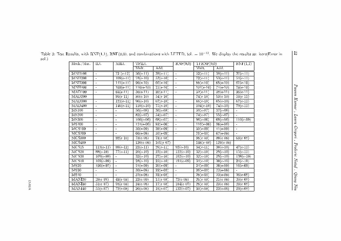
ith layer is given by v(i), the latter being the ith omponent of the ve torv = [α, β, α, β, α, β, γ, α, α], where α = 1, β = 102 and γ = 104. We haveκy = 10κx and κz = 1000κx. The velo ity eld is zero.We onsider problems on uniform grid with n×n nodes for the two-dimensional ase, where we hoose n = 100, 200, 300, and 400; whereas, for the three-dimensional ase we onsider the uniform grid with n × n × n nodes, and we hoose n = 20, 30, and 40.6.2 Comments on the numeri al testsAll our test results were obtained with GMRES(20) in double pre ision arith-meti with initial solution ve tor as ve tor of all zeros. The known solution isa random ve tor. The stopping riteria is the de rease of the relative residualbelow 10−12. The maximum number of iterations allowed is 200. The methodof NF is implemented in Fortran 90, whereas, the method of LFTFD is im-plemented in MATLAB, for this reason instead of CPU time, we provide theop ount (see Table 1) for a nx × nx × nx uniform grid for all the methods onsidered.In table 1, we introdu e short notations for the methods and the test ases onsidered.To ompare RNF(1,1) and RNF(0,0) with other lassi al methods, we presentresults in Table (3). We noti e that RNF(1,1) takes smaller number of steps to onverge as ompared to the lassi al pre onditioners like ILU and MILU. Inmost of the test ases, we observe that whenever MILU onverged within 200steps, RNF(1,1) onverged as well. For matri es with dis ontinuous oe ientslike skys rapper and onve tive skys rapper problems, RNF(1,1), ILU(0), andMILU fail to onverge within the maximum number of iterations. The on-ditioning behavior of RNF(0,0) seems to be similar to ILU(0) in terms of thenumber of steps required for onvergen e; the problems for whi h ILU(0) on-verges, RNF(0,0) onverges as well, and for those for whi h ILU(0) does not onverge, RNF(0,0) does not onverge either. These observations suggest thatRNF(0,0) alone an repla e ILU(0) for ertain problems; the advantage of doingthis is that for RNF(0,0), no ost of onstru tion is required, and there are nostorage requirements (see Table 2). On the other hand, omparing RNF(0,0)and RNF(1,0) (see table 3 and table 4), we nd that RNF(1,0) onverges fasterwhen ompared to RNF(0,0). So, RNF(1,0) an also repla e ILU(0) for the test ases onsidered. INRIA
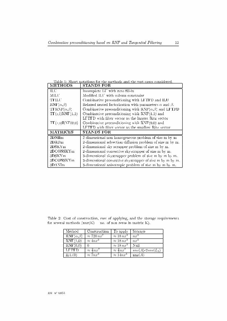
Combinative pre onditioning based on RNF and Tangential Filtering 15Table 1: Short notations for the methods and the test ases onsidered.METHODS STANDS FORILU In omplete LU with zero ll-inMILU Modied ILU with olsum onstraintTFILU Combinative pre onditioning with LFTFD and ILURNF(α,β) Relaxed nested fa torization with parameters α and β.TFRNF(α,β) Combinative pre onditioning with RNF(α,β) and LFTFDTF(r,l)RNF(1,1) Combinative pre onditioning with RNF(1,1) andLFTFD with lter ve tor as the largest Ritz ve torTF(r,s)RNF(0,0) Combinative pre onditioning with RNF(0,0) andLFTFD with lter ve tor as the smallest Ritz ve torMATRICES STANDS FOR2DNHm 2-dimensional non-homogeneous problem of size m by m2DADm 2-dimensional adve tion diusion problem of size m by m.2DSKYm 2-dimensional sky s rapper problem of size m by m.2DCONSKYm 2-dimensional onve tive skys rapper of size m by m.3DSKYm 3-dimensional skys rapper problem of size m by m by m.3DCONSKYm 3-dimensional onve tive skys rapper of size m by m by m.3DANIm 3-dimensional anisotropi problem of size m by m by m.
Table 2: Cost of onstru tion, ost of applying, and the storage requirementsfor several methods (nnz(K) = no. of non-zeros in matrix K).Method Constru tion To apply StorageRNF(α,β) ≈ 720 nx7 ≈ 18 nx3 nx3RNF(1,0) ≈ 4nx3 ≈ 18 nx3 nx3RNF(0,0) 0 ≈ 18 nx3 NullLFTFD ≈ 23nx7 ≈ 2
3nx7 nnz(A)-2nnz(L3)ILU(0) ≈ 7nx3 ≈ 14nx3 nnz(A)RR n° 6955

16 Pawan Kumar , Laura Grigori , Frederi Nataf , Qiang NiuTo study the spe trum of RNF(α,α) pre onditioned matrix for dierent val-ues of the parameter α, we display the spe trum for 30×30 skys rapper problemin the Figure (1). The spe trum of TFRNF(0,0) pre onditioned matrix is dis-played in the Figure (2). As we observe in the gure, the parameter has inuen eon the spe trum; with α = 0, the eigenvalues of RNF(0,0) lies between zero andone, whi h is favorable for the multipli ative pre onditioning as seen in se tion5. For a fair omparison, in tables 3 and 4, the number of iterations orrespond-ing to multipli ative ombination are doubled. On the other hand, the numberof iterations for the additive ase are the a tual number of iterations, keeping inmind that ea h of the pre onditioner solves an be performed on two dierentpro essors on parallel ar hite tures.0 0.1 0.2 0.3 0.4 0.5 0.6 0.7 0.8 0.9 1
−1
0
1
0 0.1 0.2 0.3 0.4 0.5 0.6 0.7 0.8 0.9 1−1
0
1
0 0.2 0.4 0.6 0.8 1 1.2 1.4−1
0
1
0 0.2 0.4 0.6 0.8 1 1.2 1.4−1
0
1
0 0.2 0.4 0.6 0.8 1 1.2 1.4 1.6 1.8−1
0
1
0 500 1000 1500 2000 2500−2
0
2x 10
−12
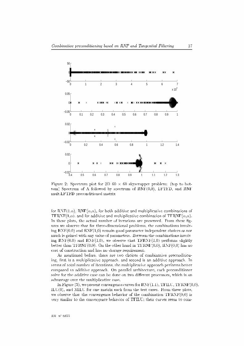
Figure 1: Spe trum plot for RNF(α, α) pre onditioned 2D 30 × 30 skys rapperproblem: (top to bottom) α = 0, 0.2, 0.4, 0.6, 0.8, and 1Comparing the ombinative pre onditioning TFILU and TFRNF(1,α), wend that the ombination TFRNF(1,α) performs mu h better ompared to the ombination TFILU or other lassi al methods (see table 3 and 4) when pa-rameter is hosen lose to 1. We noti e that the signi ant number of steps an be saved for two-dimensional problems, but for three-dimensional prob-lems dependen e on the parameter is almost negligible. This dependen e ofiteration number on the parameter for ea h type of matri es are plotted in Fig-ure (4) for two-dimensional ase and in Figure (5) for three-dimensional aseINRIA
Combinative pre onditioning based on RNF and Tangential Filtering 170 1 2 3 4 5 6 7
x 104
−50
0
50
0 0.1 0.2 0.3 0.4 0.5 0.6 0.7 0.8 0.9 1−0.05
0
0.05
0 0.2 0.4 0.6 0.8 1 1.2 1.4−0.02
0
0.02
0.4 0.5 0.6 0.7 0.8 0.9 1 1.1 1.2 1.3−0.02
0
0.02
Figure 2: Spe trum plot for 2D 60 × 60 skys rapper problem: (top to bot-tom) Spe trum of A followed by spe trum of RNF(0,0), LFTFD, and RNFmult.LFTFD pre onditioned matrixfor RNF(1,α), RNF(α,α), for both additive and multipli ative ombinations ofTFRNF(1,α), and for additive and multipli ative ombination of TFRNF(α,α).In these plots, the a tual number of iterations are presented. From these g-ures we observe that for three-dimensional problems, the ombinations involv-ing RNF(0,0) and RNF(1,0) remain good parameter independent hoi es as notmu h is gained with any value of parameters. Between the ombinations involv-ing RNF(0,0) and RNF(1,0), we observe that TFRNF(1,0) performs slightlybetter than TFRNF(0,0). On the other hand in TFRNF(0,0), RNF(0,0) has no ost of onstru tion and has no storage requirement.As mentioned before, there are two hoi es of ombinative pre ondition-ing, rst is a multipli ative approa h, and se ond is an additive approa h. Interms of total number of iterations, the multipli ative approa h performs better ompared to additive approa h. On parallel ar hite ture, ea h pre onditionersolve for the additive ase an be done on two dierent pro essors, whi h is anadvantage over the multipli ative ase.In Figure (3), we present onvergen e urves for RNF(1,1), TFILU, TFRNF(0,0),ILU(0), and MILU for one matrix ea h from the test ases. From these plots,we observe that the onvergen e behavior of the ombination TFRNF(0,0) isvery similar to the onvergen e behavior of TFILU; their urves seem to oin-RR n° 6955

18 Pawan Kumar , Laura Grigori , Frederi Nataf , Qiang Niu ide with ea h other; the reason for su h similarity may be due to the fa t thatRNF(0,0) in some sense behave as ILU(0) for all the problems onsidered (seeTable 3).Other meaningful attempt involves ombining RNF(1,1) with LFTFD wherethe lter ve tor hosen is the largest Ritz ve tor. In our test ases we observethat the reason for the failure of RNF(1,1) is the presen e of some very largeeigenvalues in the spe trum of the pre onditioned matrix, see Figure (1). Todeate one of these largest eigenvalues, we hose the lter ve tor to be thelargest Ritz ve tor obtained after 20 steps of Arnoldi iteration [6 with RNF(1,1)pre onditioned matrix. We observe that in Table (4), where the total ost isshown, this ombination is not robust enough, the reason being the presen eof many other large eigenvalues in the RNF(1,1) pre onditioned matrix whi h ause di ulties in the pre onditioned GMRES method. On the other handRNF(0,0) pre onditioned matrix has few small eigenvalues, see Figure (2). Forthis reason we hoose the lter ve tor orresponding to the smallest Ritz valuein magnitude. This ombination, i.e., TF(r,s)RNF(0,0) is not robust either, andthe reason being the presen e of other small eigenvalues in the spe trum of thepre onditioned matrix.However, in our tests we found that for the ombinative pre onditioning,the hoi e of the lter ve tor as ve tor of all ones is quite robust. Moreover, iteliminates the ost of forming the lter ve tor.
INRIA

Combinative pre onditioning based on RNF and Tangential Filtering 19
0 50 100 150 200 25010
−14
10−12
10−10
10−8
10−6
10−4
10−2
100
Convergence curves for the matrix 2dNH200200
Number of iterations
Nor
m o
f rel
ativ
e re
sidu
al
RNF(1,1)
ILU(0)+LFTFD
RNF(0,0)+LFTFD
ILU(0)
MILU(a) 2D 200 × 200 non-homogeneousproblem 0 50 100 150 200 25010
−14
10−12
10−10
10−8
10−6
10−4
10−2
100
Convergence curves for the matrix 2dAD200200
Number of iterations
Nor
m o
f rel
ativ
e re
sidu
al
RNF(1,1)
ILU(0)+LFTFD
RNF(0,0)+LFTFD
ILU(0)
MILU(b) 2D 200 × 200 adve tion diusionproblem0 50 100 150 200 250
10−14
10−12
10−10
10−8
10−6
10−4
10−2
100
Convergence curves for the matrix 2dCONSKY200200
Number of iterations
Nor
m o
f rel
ativ
e re
sidu
al
RNF(1,1)
ILU(0)+LFTFD
RNF(0,0)+LFTFD
ILU(0)
MILU( ) 2D 200×200 onve tive skys rapperproblem 0 50 100 150 200 25010
−14
10−12
10−10
10−8
10−6
10−4
10−2
100
Convergence curves for the matrix 3dSKY303030
Number of iterations
Nor
m o
f rel
ativ
e re
sidu
al
RNF(1,1)
ILU(0)+LFTFD
RNF(0,0)+LFTFD
ILU(0)
MILU(d) 3D 30×30×30 skys rapper problem
0 50 100 150 200 25010
−14
10−12
10−10
10−8
10−6
10−4
10−2
100
Convergence curves for the matrix 3dCONSKY303030
Number of iterations
Nor
m o
f rel
ativ
e re
sidu
al
RNF(1,1)
ILU(0)+LFTFD
RNF(0,0)+LFTFD
ILU(0)
MILU
(e) 3D 30×30×30 onve tive skys rap-per problem 0 10 20 30 40 50 6010
−14
10−12
10−10
10−8
10−6
10−4
10−2
100
Convergence curves for the matrix 3dANI303030
Number of iterations
Nor
m o
f rel
ativ
e re
sidu
al
RNF(1,1)
ILU(0)+LFTFD
RNF(0,0)+LFTFD
ILU(0)
MILU
(f) 3D 30×30×30 anisotropi problemFigure 3: Convergen e urves for ea h of the test problems.RR n° 6955

20 Pawan Kumar , Laura Grigori , Frederi Nataf , Qiang Niu
0 0.2 0.4 0.6 0.8 120
40
60
80
100
120
140
160
180
200
alpha
num
ber
of it
erat
ions
Plot of alpha Vs no. of iters. for 2dNH200200
RNF(1,alpha) mult. LFTFD
RNF(1,alpha) add. LFTFD
RNF(1,alpha)
(a) 2D 200 × 200 non-homogeneousproblem. 0 0.2 0.4 0.6 0.8 120
40
60
80
100
120
140
160
180
200
alpha
num
ber
of it
erat
ions
Plot of Alpha Vs No. of iters. for 2dNH200200
RNF(alpha,alpha) mult. LFTFD
RNF(alpha,alpha) add. LFTFD
RNF(alpha,alpha)
(b) 2D 200 × 200 non-homogeneousproblem.0 0.2 0.4 0.6 0.8 1
20
40
60
80
100
120
140
160
180
200
alpha
num
ber
of it
ertio
ns
Plot of alpha Vs no. of iters. for 2dAD200200
RNF(1,alpha) mult. LFTFD
RNF(1,alpha) add. LFTFD
RNF(1,alpha)
( ) 2D 200 × 200 adve tion-diusionproblem. 0 0.2 0.4 0.6 0.8 120
40
60
80
100
120
140
160
180
200
alpha
num
ber
of it
erat
ions
Plot of Alpha Vs No. of iters. for 2dAD200200
RNF(alpha,alpha) mult. LFTFD
RNF(alpha,alpha) add. LFTFD
RNF(alpha,alpha)
(d) 2D 200 × 200 adve tion-diusionproblem.0 0.2 0.4 0.6 0.8 1
20
40
60
80
100
120
140
160
180
200
alpha
num
ber
of it
erat
ions
Plot of alpha Vs no. of iters. for 2dSKY200200
RNF(1,alpha) mult. LFTFD
RNF(1,alpha) add. LFTFD
RNF(1,alpha)
(e) 2D 200×200 skys rapper problem. 0 0.2 0.4 0.6 0.8 120
40
60
80
100
120
140
160
180
200
alpha
num
ber
of it
erat
ions
Plot of alpha Vs no. of iters. for 2dSKY200200
RNF(alpha,alpha) mult. LFTFD
RNF(alpha,alpha) add. LFTFD
RNF(alpha,alpha)
(f) 2D 200×200 skys rapper problem.Figure 4: Alpha Vs number of iterations for 2D test ases.INRIA
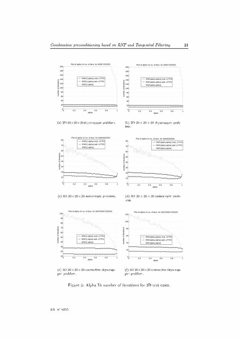
Combinative pre onditioning based on RNF and Tangential Filtering 21
0 0.2 0.4 0.6 0.8 10
20
40
60
80
100
120
140
160
180
200
alpha
num
ber
of it
erat
ions
Plot of alpha Vs no. of iters. for 3dSKY202020
RNF(1,alpha) mult. LFTFD
RNF(1,alpha) add. LFTFD
RNF(1,alpha)
(a) 3D 20×20×20 skys rapper problem. 0 0.2 0.4 0.6 0.8 10
20
40
60
80
100
120
140
160
180
200
alpha
num
ber
of it
erat
ions
Plot of alpha Vs no. of iters. for 3dSKY202020
RNF(alpha,alpha) mult. LFTFD
RNF(alpha,alpha) add. LFTFD
RNF(alpha,alpha)
(b) 3D 20× 20× 20 skys rapper prob-lem.0 0.2 0.4 0.6 0.8 1
0
10
20
30
40
50
60
70
80
alpha
num
ber
of it
erat
ions
Plot of alpha Vs no. of iters. for 3dANI202020
RNF(1,alpha) mult. LFTFD
RNF(1,alpha) add. LFTFD
RNF(1,alpha)
( ) 3D 20×20×20 anisotropi problem. 0 0.2 0.4 0.6 0.8 10
10
20
30
40
50
60
70
80
alpha
num
ber
of it
erat
ions
Plot of alpha Vs no. of iters. for 3dANI202020
RNF(alpha,alpha) mult. LFTFD
RNF(alpha,alpha) add. LFTFD
RNF(alpha,alpha)
(d) 3D 20× 20× 20 anisotropi prob-lem.0 0.2 0.4 0.6 0.8 1
10
20
30
40
50
60
70
80
90
100
alpha
num
ber
of it
erat
ions
Plot of alpha Vs no. of iters. for 3dCONSKY202020
RNF(1,alpha) mult. LFTFD
RNF(1,alpha) add. LFTFD
RNF(1,alpha)
(e) 3D 20×20×20 onve tive skys rap-per problem. 0 0.2 0.4 0.6 0.8 10
20
40
60
80
100
120
alpha
num
ber
of it
erat
ions
Plot of alpha Vs no. of iters. for 3dCONSKY202020
RNF(alpha,alpha) mult. LFTFD
RNF(alpha,alpha) add. LFTFD
RNF(alpha,alpha)
(f) 3D 20×20×20 onve tive skys rap-per problem.Figure 5: Alpha Vs number of iterations for 3D test ases.RR n° 6955
22PawanKumar,LauraGrigori,Frederi Nataf,QiangNiu
Table 3: Test Results, with RNF(1,1), RNF(0,0), and ombinations with LFTFD, tol. = 10−12. We display the results as: iters(Error insol.) Meth./Mat. ILU MILU TFILU RNF(0,0) TFRNF(0,0) RNF(1,1)Mult. Add. Mult. Add.2dNH100 - 72 (e-12) 56(e-11) 39(e-11) - 52(e-11) 38(e-11) 37(e-11)2dNH200 - 109(e-11) 78(e-10) 53(e-10) - 72(e-11) 53(e-11) 54(e-11)2dNH300 - 141(e-11) 96(e-10) 66(e-10) - 88(e-10) 65(e-10) 67(e-10)2dNH400 - 169(e-11) 110(e-10) 75(e-10) - 104(e-10) 74(e-10) 78(e-10)2dAD100 - 65(e-11) 56(e-11) 39(e-11) - 52(e-11) 38(e-11) 36(e-11)2dAD200 - 95(e-11) 80(e-10) 54(e-10) - 74(e-10) 53(e-10) 53(e-11)2dAD300 - 121(e-11) 96(e-10) 67(e-10) - 88(e-10) 65(e-10) 67(e-11)2dAD400 - 146(e-11) 110(e-10) 75(e-10) - 104(e-10) 74(e-10) 79(e-11)2dS100 - - 56(e-08) 36(e-08) - 50(e-07) 37(e-08) -2dS200 - - 82(e-07) 54(e-07) - 74(e-07) 55(e-07) -2dS300 - - 100(e-06) 68(e-07) - 96(e-06) 69(e-06) 110(e-09)2dS400 - - 124(e-06) 82(e-06) - 116(e-06) 86(e-06) -2dCS100 - - 50(e-09) 39(e-09) - 50(e-09) 41(e-09) -2dCS200 - - 66(e-08) 59(e-09) - 76(e-08) 67(e-08) -2dCS300 - 92(e-10) 78(e-08) 73(e-08) - 98(e-08) 80(e-08) 63(e-08)2dCS400 - - 120(e-08) 101(e-07) - 138(e-08) 120(e-08) -3dCS15 113(e-11) 99(e-12) 22(e-11) 28(e-11) 92(e-10) 34(e-11) 30(e-10) 47(e-11)3dCS20 88(e-10) 77(e-11) 20(e-10) 23(e-10) 122(e-10) 32(e-10) 29(e-10) 15(e-11)3dCS30 169(e-09) - 32(e-10) 27(e-10) 162(e-10) 32(e-10) 29(e-10) 138(e-10)3dCS40 169(e-09) - 28(e-10) 25(e-10) 191(e-09) 34(e-10) 30(e-10) 24(e-10)3dS20 196(e-07) - 24(e-09) 20(e-09) - 24(e-09) 20(e-09) 16(e-09)3dS30 - - 30(e-08) 22(e-08) - 26(e-08) 22(e-08) -3dS40 - - 32(e-08) 23(e-08) - 28(e-08) 23(e-08) 26(e-08)3dANI20 29(e-08) 43(e-08) 22(e-09) 15(e-08) 72(e-08) 26(e-08) 21(e-08) 20(e-08)3dANI30 51(e-07) 58(e-08) 24(e-08) 17(e-08) 104(e-07) 28(e-08) 23(e-08) 23(e-08)3dANI40 55(e-07) 72(e-08) 26(e-08) 18(e-07) 132(e-07) 30(e-08) 23(e-08) 23(e-08)INRIA

Combinativepre onditioning
basedonRNFandTangentia
lFiltering23 Table 4: Test Results, with RNF(1,1), RNF(0,0), RNF(1,0), and ombinations with LFTFD, tol. = 10−12. We display the results as:iters(Error in sol.)Meth./Mat. RNF(1,0) TFRNF(1,0) TFRNF(.9,.9) TFRNF(1,0.9) TF(r,l)RNF(1,1) TF(r,s)RNF(0,0)Mult. Add. Mult. Add. Mult. Add. Mult. Mult.2dNH100 168(e-10) 48(e-11) 35(e-11) 36(e-11) 24(e-11) 34(e-11) 21(e-10) 52(e-11) 52(e-11)2dNH200 - 70(e-11) 48(e-10) 50(e-10) 34(e-11) 48(e-10) 29(e-10) 78(e-11) -2dNH300 - 84(e-10) 59(e-10) 62(e-10) 40(e-10) 58(e-10) 36(e-10) 104(e-10) -2dNH400 - 96(e-10) 69(e-10) 72(e-10) 46(e-10) 70(e-10) 42(e-10) 122(e-10) -2dAD100 168(e-10) 48(e-11) 35(e-11) 36(e-11) 24(e-11) 32(e-11) 21(e-10) 52(e-11) 52(e-11)2dAD200 - 70(e-11) 49(e-10) 50(e-10) 33(e-10) 48(e-10) 30(e-10) 78(e-11) 394(e-09)2dAD300 - 84(e-10) 59(e-10) 64(e-10) 40(e-10) 60(e-10) 37(e-10) 100(e-10) -2dAD400 - 96(e-10) 67(e-10) 70(e-10) 45(e-10) 70(e-10) 42(e-10) 128(e-10) -2dS100 - 44(e-07) 33(e-08) 42(e-07) 22(e-07) 42(e-07) 23(e-07) - -2dS200 - 68(e-07) 51(e-07) 64(e-07) 32(e-07) 60(e-07) 30(e-07) - -2dS300 - 84(e-06) 60(e-07) 58(e-06) 38(e-06) 56(e-07) 34(e-06) 124(e-09) -2dS400 - 102(e-06) 72(e-06) 94(e-06) 47(e-06) 92(e-06) 46(e-06) - -2dCS100 - 46(e-09) 39(e-09) 38(e-09) 31(e-09) 38(e-09) 32(e-09) - 390(e-09)2dCS200 - 70(e-08) 57(e-08) 52(e-09) 39(e-08) 52(e-08) 39(e-09) - -2dCS300 - 80(e-08) 73(e-08) 56(e-08) 43(e-08) 48(e-08) 39(e-08) 108(e-09) -2dCS400 - 124(e-07) 109(e-07) 74(e-08) 59(e-08) 72(e-08) 58(e-08) - -3dCS15 92(e-10) 30(e-11) 28(e-10) 44(e-10) 36(e-11) 48(e-11) 37(e-11) 76(e-11) 154(e-10)3dCS20 97(e-10) 30(e-11) 27(e-10) 28(e-10) 27(e-11) 28(e-10) 26(e-11) 30(e-11) 302(e-10)3dCS30 168(e-09) 28(e-10) 26(e-10) 44(e-10) 29(e-10) 44(e-10) 29(e-10) - 120(e-09)3dCS40 - 28(e-10) 27(e-10) 26(e-10) 24(e-09) 24(e-09) 24(e-10) 78(e-10) 170(e-09)3dS20 - 24(e-09) 20(e-09) 26(e-09) 20(e-09) 26(e-09) 20(e-09) 28(e-09) 278(e-08)3dS30 - 26(e-08) 22(e-08) 50(e-09) 25(e-09) 52(e-09) 26(e-08) - 188(e-08)3dS40 - 28(e-08) 22(e-08) 30(e-08) 21(e-08) 32(e-09) 21(e-08) 46(e-09) -3dANI20 57(e-08) 26(e-09) 19(e-08) 18(e-08) 14(e-08) 18(e-08) 13(e-08) 28(e-09) 84(e-09)3dANI30 75(e-07) 28(e-08) 21(e-08) 20(e-08) 15(e-08) 20(e-08) 14(e-08) 30(e-08) 72(e-06)3dANI40 106(e-07) 28(e-08) 22(e-08) 20(e-07) 15(e-07) 20(e-08) 14(e-08) 32(e-08) 84(e-08) RRn°6955

24 Pawan Kumar , Laura Grigori , Frederi Nataf , Qiang Niu7 CONCLUSIONAND FUTURE DIRECTIONSWe have introdu ed a relaxed version of NF, and an ee tive ombinative pre- onditioning is a hieved in ombination with tangential ltering pre onditioners[4. Compared to ILU(0), it has several important properties. If A is S.P.D.then RNF(0,0)is S.P.D. and leads to a stable splitting. There is no setup ostnor storage requirement. The new pre onditioner is parti ularly useful whenmultipli ate/additive pre onditioning is a hieved in ombination with tangen-tial ltering pre onditioner [4. With this setup the new pre onditioner is asrobust as the ombination of ILU(0)with tangential ltering pre onditioner.A future work onsists in studying other modied version of NF, similar toone suggested by Gustason [13, [14 for MILU, where the diagonal is perturbedby an additive term of order O(h2), whi h seems to improve the onditioning ofmodied in omplete fa torization methods for ertain lass of problems.Referen es[1 J. R. Appleyard and I. M. Cheshire, Nested Fa torization, SPE 12264,presented at the Seventh SPE Symposium on Reservoir Simulation, SanFran is o, 1983.[2 J. R. Appleyard, Proof that simple Colsum modied ILU fa toriza-tion of matri es arising in Fluid folw problems are not singular, byJohn Appleyard, Polyhedron Software Ltd, May 2004. Available online :http://www.polyhedron. om/ olsum-proof.[3 J. R. Appleyard and I. M. Cheshire, Stri tly Triangular L.U formulation ofNested Fa torization, by John Appleyard, Polyhedron Software Ltd, May2004. Available online : http://www.polyhedron. om/stri tlu.[4 Y. A hdou and F. Nataf, Low frequen y tangential ltering de omposition,Numer. Linear Algebra Appl., 14, (2007), pp. 129-147.[5 S. F. Ashby, M. J. Holst, T. A. Manteuel, and P. E. Saylor The role ofinner produ t in stopping riteria for onjugate gradient iterations, BIT.,41, (2001), pp. 26-52.[6 Z. Bai, J. Demmel, J. Dongarra, A. Ruhe, and H. van der Vorst Tem-plates for the Solution of Algebrai Eigenvalue Problems: A Pra ti al Guide,SIAM, Philadelphia, 2000.[7 M. Benzi, A. M. Tuma, A omparative study of sparse approximate inversepre onditioners, Appl. Numer. Math., 30, (1999), pp. 305-340.[8 D. Braess Towards algebrai multigrid for ellipti problems of se ond order,Computing, 55(4), (1995), pp. 379-393.[9 A. Buzdin, Tangential de omposition, Computing., 61, (1998), pp. 257-276.[10 A. Buzdin and G. Wittum, Two-frequen y de omposition, Numer. Math.,97, (2004), pp. 269-295. INRIA
Combinative pre onditioning based on RNF and Tangential Filtering 25[11 C. Wagner and G. Wittum, Adaptive ltering, Numer. Math., 78, (2004),pp. 305-328.[12 P. A. Crumpton, P. A. Fjerstad, and J. Berge, Parallel omputing UsingECLIPSE Parallel S hlumberger, E lipse, Te hni al Des ription 2003A,Chapter 38: Parallel Option. 2003.[13 Gustafsson I, A lass of rst order fa torization methods, BIT 18, pp. 142-56, 1978.[14 Gustafsson I, Modied in omplete holesky(MIC) methods, In D.Evans, ed-itor, Pre onditioning Methods-Theory and Appli ations, pp. 265-293. Gor-don and Brea h, New York, 1983.[15 N. N. Kuznetsova, O. V. Diyankov, S. S. Kotegov, S. V. Koshelev, I. V.Krasnogorov, V. Y. Pravilnikov, and S. Y. Maliassov, The family of nestedfa torizations, Russian Journal of Numeri al Analysis and Mathemati alModelling. 22(4) (2007), pp. 393â412.[16 G. Meurant Computer Solution of Large Linear Systems North-HollandPublishing Co. Amsterdam, 1999.[17 J. W. Ruge, K. Stüben Algebrai multigrid. Multigrid Methods, Frontiersof Applied Mathemati s, vol. 3. SIAM Philadelphia, PA, 1987; 73â130.[18 Y. Saad, Iterative Methods for Sparse Linear Systems, PWS publishing ompany, Boston, MA, 1996.[19 K. Stüben, A review of algebrai multigrid, J. Comput. Appl. Math. andapplied mathemati s, 128(1-2), (2001), pp. 281-309, Numeri al analysis2000, vol. VII, Partial dierential equations.[20 U. Trottenberg, C. W. Oosterlee, and A. S hüller, Multigrid, A ademi Press In . San Diego, CA, (2001). With ontributions by Brandt A, OswaldP, and Stüben K.[21 C. Wagner, Tangential frequen y ltering de ompositions for symmetri matri es, Numer. Math., 78, (1997), pp. 119-142.[22 C. Wagner, Tangential frequen y ltering de ompositions for unsymmetri matri es Numer. Math., 78, (1997), pp. 143-163.[23 C. Wagner and G. Wittum, Adaptive ltering, Numer. Math., 78, (1997),pp. 305-382.[24 P. Van¥k, M. Brezina, and J. Mandel Convergen e of algebrai multigridbased on smoothed aggregation, Numeris he Mathematik, 88(3), (2001), pp.559-579.[25 L. Grigori, F. Nataf, and Q. Niu, Two sides tangential ltering de omposi-tion, INRIA TR 6554.RR n° 6955

Centre de recherche INRIA Saclay – Île-de-FranceParc Orsay Université - ZAC des Vignes
4, rue Jacques Monod - 91893 Orsay Cedex (France)
Centre de recherche INRIA Bordeaux – Sud Ouest : Domaine Universitaire - 351, cours de la Libération - 33405 Talence CedexCentre de recherche INRIA Grenoble – Rhône-Alpes : 655, avenue de l’Europe - 38334 Montbonnot Saint-Ismier
Centre de recherche INRIA Lille – Nord Europe : Parc Scientifique de la Haute Borne - 40, avenue Halley - 59650 Villeneuve d’AscqCentre de recherche INRIA Nancy – Grand Est : LORIA, Technopôle de Nancy-Brabois - Campus scientifique
615, rue du Jardin Botanique - BP 101 - 54602 Villers-lès-Nancy CedexCentre de recherche INRIA Paris – Rocquencourt : Domaine de Voluceau - Rocquencourt - BP 105 - 78153 Le Chesnay CedexCentre de recherche INRIA Rennes – Bretagne Atlantique : IRISA, Campus universitaire de Beaulieu - 35042 Rennes Cedex
Centre de recherche INRIA Sophia Antipolis – Méditerranée :2004, route des Lucioles - BP 93 - 06902 Sophia Antipolis Cedex
ÉditeurINRIA - Domaine de Voluceau - Rocquencourt, BP 105 - 78153 Le Chesnay Cedex (France)http://www.inria.fr
ISSN 0249-6399