COMA Control Engineering with Maxima - Austromath · Control Engineering with Maxima Wilhelm Haager ... is passed to Gnuplot via the option user_preamble in appropriate form

,d�>µs��^�X�W�o��v ÇÅÄÄ�^�X�W�o��v�n�t�o��Ç�n�ÄÆËÈÆ-ËÉÄÉÅ-ÇÄÄ

�o�l��}��Zv]l ��Z�o��X��X��n�Z��Wll��XZ�o��X��X��

,�Z��]oµvP�n�&��Z��Zµo��n��v��Zµo�

COMAControl Engineering with Maxima

Wilhelm Haager

HTL St. Pölten, Department Electrical Engineering

[email protected]

Version 1.8, April 18, 2017

Contents 2

Contents

1 Introduction 31.1 Notions . . . . . . . . . . . . . . . . . . . . . . . . . . . . . . . . . . . . . . . . . . . . . . . 31.2 wxMaxima User Interface . . . . . . . . . . . . . . . . . . . . . . . . . . . . . . . . . . . 41.3 Basic Concepts of the Package COMA . . . . . . . . . . . . . . . . . . . . . . . . . . . . 4

2 Plot routines 52.1 Options of the Gnuplot-Interface Draw . . . . . . . . . . . . . . . . . . . . . . . . . . . 52.2 Additional Options of COMA . . . . . . . . . . . . . . . . . . . . . . . . . . . . . . . . . 62.3 Plot . . . . . . . . . . . . . . . . . . . . . . . . . . . . . . . . . . . . . . . . . . . . . . . . . 62.4 Contour Lines . . . . . . . . . . . . . . . . . . . . . . . . . . . . . . . . . . . . . . . . . . . 8

3 Transfer functions 9

4 Laplace Transformation, Step Response 13

5 Frequency Responses 15

6 Investigations in the Complex s-Plane 206.1 Poles/Zeros-Distribution . . . . . . . . . . . . . . . . . . . . . . . . . . . . . . . . . . . . 206.2 Root Locus Plots . . . . . . . . . . . . . . . . . . . . . . . . . . . . . . . . . . . . . . . . . 21

7 Stability Behavior 237.1 Stability . . . . . . . . . . . . . . . . . . . . . . . . . . . . . . . . . . . . . . . . . . . . . . . 237.2 Relative Stability . . . . . . . . . . . . . . . . . . . . . . . . . . . . . . . . . . . . . . . . . 25

8 Optimization 27

9 Controller Design 28

10 State Space 30

11 Various Functions 34

Bibliography 35

Wilhelm Haager: Control Engineering with Maxima

1 Introduction 3

1 Introduction

1.1 Notions

Maxima: Open-Source descendant of the computeralgebra system Macsyma, which initially wasdeveloped 1967–1982 at the MIT by order of the US Department of Energy. 1989 a versionof Macsyma was published with the name Maxima under the GNU General Public Licence,which is now being developed further by an independent group of users. Maxima is writtenin Lisp and contains many aspects of functional programming.

Due to its power and free availability there is no reason to use it not.wxMaxima: One of several graphical user interfaces for Maxima. It enables input and editing

expressions in a working window, as well as the documenting calculations with text andimages. Maxima outputs results and (on demand) graphics into that working window.

Working sessions can be saved, loaded and re-executed; the most common commands areaccessible via menus and control buttons (for notorious mouse-clickers) . Working sessionscan be exported as HTML or as LATEX-file. Export to LATEX may require some corrections byhand of the resulting TEX-file.

On installing Maxima, wxMaxima is automatically installed as the standard user interface.

COMA (COntrol engineering with MAxima):

Control engineering package for Maxima, it comprises basic methods for system analysis intime-, frequency- and Laplace-domain, controller design, as well as state space methods:

• Inverse Laplace-transform of transfer functions of arbitrary order (the built-in func-tion ilt in general fails at orders higher than two).

• Unit step responses

• Nyquist diagrams and Bode plots

• Poles and Zeros, root locus plots

• Stability investigations: stability limit, Hurwitz criterion, stable regions in the param-eter plane, phase margin, gain margin

• Optimization and controller design: ISE-criterion (integral of squared error), gainoptimum

• State space: Conversion into a transfer function, canonical forms, controllability, ob-servability


1 Introduction 4

1.2 wxMaxima User Interface

À . . . Working window for input and outputÁ . . . Gnuplot output window

1.3 Basic Concepts of the Package COMA

• The Laplace variable is considered to be always s, the time variable always t; in functionsconcerning the frequency response, the angular frequency is ω. In frequency responses sis automatically replaced by jω. Transfer functions are rational functions in the variable s,time delays are not supported, but can be approximated by Padé approximations.

• All functions, which take a transfer function as a parameter, can also take (without explicitnotice) a list of transfer functions as a parameter; in that case the result will also be a list,of which the elements correspond to the particular transfer functions. That is particularlyimportant in graphics, where a couple of curves shall be drawn into a single diagram.

The list to be plotted need not have only functions (transfer functions), but can alsocontain graphic objects of the Gnuplot interface Draw (explicit, points, implicit,parametric, polar, polygon, rectangle, ellipse, label). Thus diagrams can be pro-vided with labels, legends and other graphical elements; furthermore a direct comparisonwith measured values is possible.

• Additional to the plotted functions, all plot routines can have optional parameters in theform option = value, which allow to adapt the graphic with respect to colors, line widths,scale, graphic type, output etc.

• Priot to its first usage, the package has to be laded using the command load.


2 Plot routines 5

2 Plot routines

Maxima uses the program Gnuplot [2] for drawing graphics, which is called at the generationof the graphic. Herein the graphic is drawn either in a seperate Gnuplot window (using theoption wx=false) or directly into the working window of wxMaxima (using the option wx=true,default).

The plot routines of COMA don’t use the standard functions of Maxima (plot2d, plot3d,wxplot2d, wxplot3d), but the functions of the additional package Draw (draw2d, draw3d,wxdraw2d und wxdraw3d), refer [1], [3]. Those functions are a little bit more complicatedin their application, but they offer much more possibilities to adapt the graphics according tospecial requirements by the use of options.

All plot routines take a single function as parameter or a list of functions; additional optionalparameters in the form option=value. Options, which apply to particular graphic objects, (color,line_width etc.), can be given in a list, of which the elements correspond to the respectivegraphic objects: option=[val1,val2, . . . ].

2.1 Options of the Gnuplot-Interface Draw

terminal=target output target, possible values: screen (default), jpg,png, pngcairo, eps, eps_color

file_name=string name of the output file, default: maxima_out.ext

color=c plot color

line_width=w line width

xrange=[x1,x2] plot range in x-direction

yrange=[x1,y2] plot range in y-direction

zrange=[z1,z2] plot range in z-direction

logx=true/false logarithmic scale of the x-axis

logy=true/false logarithmic scale of the y-axis

logz=true/false logarithmic scale of the z-axis

grid=true/false inclusion of grid lines

enhanced3d=true/false coloring of surfaces in 3D-plots

Important options of the Gnuplot-interface Draw

A complete list of the options can be found in in the Maxima manual [1].


2 Plot routines 6

2.2 Additional Options of COMA

wx=true/false determines the output:true . . . output into the wxMaxima working windowfalse . . . output into a seperate Gnuplot window

aspect_ratio=value ratio height/width of the diagram; the value −1 resultsin same scale of the x-axis and the y-axis

color=[c1,c2,. . . ] list of colors, which are applied for the particularelements to be plotted respectively

line_width=[w1,w2,. . . ] list of linewidths, applied to the elements respectively

dimensions=[width,height] width and height of the graphic...

Global variable:

coma_defaults list containing options in the form option=value

Additional options of COMA

The variable coma_defaults is a list containing default values for settings in the form of key-value pairs. Contrary to the list draw_defaults of the Gnuplot-interface Draw coma_defaultscan contain also othe options, which are not part of Draw.

2.3 Plot

The function plot performs a two-dimensional depiction of functions f (x) in one variable or athree-dimensional depiction of functions f (x , y) in two variables.

plot(f(x), opts) plotting the function f (x) in a two-dimensionalcoordinate system

plot(f(x,y), opts) plotting the function f (x , y) in 3D-representation

Instead of a single function f , also a list of functions[ f1, f2, . . . ] can be plotted.

Plot routines for 2D und 3D graphics

The functions of the package Draw (wxdraw2d, draw2d, wxdraw3d, draw3d) are called inter-nally with appropriate parameters. Thus the (convenient) call of

plot([f(x),g(x)],xrange=[0,10],color=[red,blue])

exactly corresponds to the (less convenient) command

wxdraw2d(xrange=[0,10],color=red, explicit(f(x),x,0,10),

color=blue, explicit(g(x),x,0,10)).


2 Plot routines 7

The value of the option aspect_ratio, which does not exist in the routines of the packageDraw, is passed to Gnuplot via the option user_preamble in appropriate form.

Loading the control engineering package (%i1) load(coma)$

coma v.1.84, (Wilhelm Haager, 2017−02−24)

List containing default values for thegraphics options

(%i2) coma_defaults ;

(%o2) [grid�true ,wx�true ,dimensions �[600 ,350 ],user_preamble �set grid linetype 3 lc '#444444' ,color�[red ,blue ,dark −green ,goldenrod ,violet ,gray40 ,dark −cyan ,orange ,brown ,sea −green ]]

List of color names (%i3) col:[red,green,brown,blue];

(%o3) [red ,green ,brown ,blue ]

Plotting a list of four functions in onesingle variable; internally the functionwxdraw2d is called. The names of thevariables can be different in eachfunction.

(%i4) plot([sin(5*x)**2,0.8*sin(5*y)**2,x,0.8*y],xrange=[-0.5,1.5],color=col,line_type =[solid,solid,dots,dots]);

(%t4)

Plotting a list of two functions in twovariables each; internally the functionwxdraw3d is called.The option surface_hide=truesuppresses hidden lines.

(%i5) plot([sin(5*x)**2+0.8*sin(5*y)**2,x+0.8*y],xrange=[-0.5,1.5],surface_hide =true)$

(%o4) (%t5)

plot evaluates the function to be plotted f before points are calculated. In order to evaluatethe function for every particular point, it has to be quoted. That is especially important e.g. forcharacteristic values of transfer functions (section 7), which can only be calculated numerically.

Transfer function with a dependence ona parameter a

(%i6) f:(s+a)/(s^3+a*s^2+2*s+a);

(%o6) s�a

s3�a s

2�2 s�a


2 Plot routines 8

The damping can only be calculatednumerically, which requires a to have afixed value. Thus f has to be quoted toavoid being evaluated too early.

(%i7) plot('damping_ratio (f),xrange=[0,5]);

(%t7)

2.4 Contour Lines

The function contourplot draws isolines of a function f (x , y). Contrary to contour_plot,which is part of Maxima, it uses the Gnuplot interface Draw, like all plot routines of the packageCOMA. It also has the same options.

contourplot(f(x,y), x , y, opts) Plotting of isolines of the function f (x , y)

contours=[z1, z2, . . . ] Determining the function values for the isolines

Contour Lines

Transfer function with two parameters aand b

(%i8) f:1/(s^5+s^4+5*s^3+a*s^2+b*s+1);

(%o7)

(%o8) 1

s5�s

4�5 s

3�a s

2�b s�1

Isolines for the damping in dependenceon the parameters a and b. The blackline at damping 0 represents the stabilitylimit, green lines represent stable areas,red lines unstable areas.

(%i9) contourplot ('damping (f),a,b,xrange=[0,8], yrange=[0,7],contours =[-0.3,-0.2,-0.1,0,0.1],color=[red,red,red,black,green],ip_grid_in =[20,20])$

(%t9)



3 Transfer functions

COMA provides the following functions for convenient generation of transfer functions, primarilyfor testing and experimenting:

rantranf(n) n-th order random transfer function, of wich thenumerator and denominator coefficients are numbersbetween 1 and 10

stable_rantranf(n) Stable random transfer function (only up to 6th order)

gentranf(c, k, d, n) n-th order transfer function, (numerator of k-th order)with the numerator coefficients ci and the denominatorcoefficients di

tranftype(F(s)) Type of the transfer function F(s) as a string

ntranfp(F(s)) Yields true, if all coefficients of the transfer functionF(s) evaluate to numbers.

closed_loop(Fo(s)) Calculation of the closed loop transfer function FW (s)from the open loop FO(s)

open_loop(Fw(s)) Calculation of the open loop transfer function FO(s)from the closed loop FW (s)

time_delay(T, n, [k]) n-th order Padé approximation for a time delay system.The order of the numerator k is optional.

impedance_chain(Z1, Z2, . . . [n])transfer function of an impedance chain with theimpedances Z1, Z2, . . . and an (optional) repeat factorn

transfer_function(eqs, vars, u, y)Calculation of the transfer function from the equationseqs in the variables vars with the inputs u and theoutputs y

sum_form(F(s), n) One of four canonical forms F(s) (in depoendence of n)

product_form(F(s), [n]) Splitting up F(s) into linear und quadratic factors

Generation of transfer cunctions

The function stable_rantranf(n) searches denominator coefficients randomly between 1and 10, until a stable transfer function is found, which is becoming more difficult at higherorders, at seventh order computing time is increasing heavily. Thus stable_rantranf is work-ing only for transfer functions up to sixth order.

Higher orders can be attained by multiplication of several lower order transfer functions. How-ever, in that case the coefficients are not confined to the range 1. . . 10 any more.



Generation of a list of fourth orderrandom transfer functions, the orders onthe numerators are lower, at least byone.

(%i1) fli:makelist (rantranf (3),k,1,4);

(%o1) [4 s

2�8 s�10

4 s3�s

2�4 s�10

,9 s�10

7 s3�7 s

2�2 s�4

,

2 s2�10 s�7

4 s3�5 s

2�9 s�7

,2 s

2�s�10

10 s3�10 s

2�2 s�5

]

Stability test of the transfer functions(section 7)

(%i2) stablep (fli);

(%o2) [false ,false ,true ,false ]

Generation of a list of stable randomtransfer functions

(%i3) fli:makelist (stable_rantranf (3),k,1,4);

(%o3) [3

2 s3�10 s

2�7 s�4

,4 s

2�10 s�1

2 s3�3 s

2�6 s�4

,

8 s�7

2 s3�9 s

2�s�1

,10

4 s3�10 s

2�4 s�5

]

All are stable. (%i4) stablep (fli);

(%o4) [true ,true ,true ,true ]

List of transfer functions (%i5) fo:[k/s,5/(s*(s+3)),1-b/s];

(%o5) [k

s,

5

s� �

s�3,1−

b

s]

Calculation of the closed loop transferfunctions

(%i6) fw:closed_loop (fo);

(%o6) [k

s�k,

5

s2�3 s�5

,s−b

2 s−b]

Determining the types of the transferfunctions as strings

(%i7) tranftype (fw);

(%o7) [PT1 ,PT2 ,PDT1 ]

Check, whether all coefficients of thetransfer functions evaluate to numbers

(%i8) ntranfp (fw);

(%o8) [false ,true ,false ]

Back-calculation to the open looptransfer functions

(%i9) open_loop (fw);

(%o9) [k

s,

5

s2�3 s

,s−b

s]

gentranf(a,k,b,n) produces a general transfer function with indexed coefficients in the form

a0 + a1s+ a2s2 + · · ·+ aksk

b0 + b1s+ b2s2 + · · ·+ bnsn.

transfer function with generalcoefficients ai and bi

(%i10) gentranf (a,3,b,5);

(%o10) a3s3�a

2s2�a

1s�a

0

b5s5�b

4s4�b

3s3�b

2s2�b

1s�b

0

Time delay systems have transcendental transfer functions, inverse Laplace transform of controlloops containing time delays is not possible analytically in general.time_delay(T,n,k) yields a n-th order Padé approximation of a time delay system with thetransfer function G(s)=e−sT . The declaration k of the numerator order is optional, its default isn− 1.



Fourth order Padé approximation of thetransfer function of a time delayG(s)=exp(−sT )

(%i11) time_delay (T,4);

(%o11) −4 T

3s3�60 T

2s2−360 T s�840

T4s4�16 T

3s3�120 T

2s2�480 T s�840

impedance_chain calculates the transfer function of an impdance chain with arbitrary impedances(of even number); the last (optional integer valued) parameter determines the number of repe-titions of the impedance chain.

Z1 Z3 Zn−1

Z2 Z4 ZnUE(s) UA(s)

transfer function of an impedance chainconsisting of four elements

(%i12) impedance_chain (R,1/(s*C),s*L+R,1/(s*C));

(%o12) 1

C2L R s

3�

� �

C2R2�C L s

2�3 C R s�1

transfer function of an impedance chainrepeated four times

(%i13) impedance_chain (R,1/(s*C),4);

(%o13) 1

C4R4s4�7 C

3R3s3�15 C

2R2s2�10 C R s�1

transfer_function(eqs,vars,u,y) calculates the transfer function from a list of linear equa-tions eqs, e.g. from a block diagram. vars is a list containing the used variables according towhich the system of equations is to be solved, u is the input, y is the output.Also multivariable systems can be calculated: When u and y are lists of variables, the corre-sponding transfer matrix is calculated.

u F2 y

F1

F3

x2

x1

x3

−

x1 = F1 · ux2 = F2 · (u− x3)

x3 = F3 · yy = x1 + x2

System of linear equations from theblock diagram

(%i14) eqs:[x1=F1*u,x2=F2*(u-x3),x3=F3*y,y=x1+x2];

(%o14) [x1�F1 u,x2�F2� �

u−x3 ,x3�F3 y,y�x2�x1]

Calculation of the transfer function fromthe equations

(%i15) transfer_function (eqs,[x1,x2,x3,y],u,y);

(%o15) F2�F1

F2 F3�1

sum_form(F(s),n) divides the numerator and the denominator of F(s) in dependence of n by apartitcular coefficient, thus making one of the leading or last coefficients to 1:

n= 1 . . . leading numerator coefficient of F(s)n= 2 . . . last numerator coefficient of F(s)n= 3 . . . leading denominator coefficient of F(s)n= 4 . . . last denominator coefficient of F(s) (default)



(%i16) F:(2*s+3)/(4*s^3+5*s^2+6*s+7);

(%o16) 2 s�3

4 s3�5 s

2�6 s�7

Canonical forms, making the leading orlast numerator coefficient to 1:

(%i17) [sum_form (F,1),sum_form (F,2)];

(%o17) [s�1.5

2 s3�2.5 s

2�3 s�3.5

,

0.66667 s�1

1.3333 s3�1.6667 s

2�2 s�2.3333

]

Canonical forms, making the leading orlast denominator coefficient to 1:

(%i18) [sum_form (F,3),sum_form (F,4)];

(%o18) [0.5 s�0.75

s3�1.25 s

2�1.5 s�1.75

,

0.28571 s�0.42857

0.57143 s3�0.71429 s

2�0.85714 s�1

]

product_form splits numerator and denominator of the transfer function into linear and quadraticfactors:

Product form of a transfer function (%i19) product_form (F);

(%o19) 0.42857

� �

0.66667 s+1.0� �

0.82799 s+1.0

� �

0.69014 s2+0.029158 s+1.0



4 Laplace Transformation, Step Response

Maxima provides the function laplace(f,t,s) for the Laplace transform; the inverse Laplacetransform is calculated with ilt(f,s,t). The coefficients of the numerator and denominatorpolynomials can have symbolic values. However, ilt fails at denominator polynomials of thirdor higher order, if no zeros can be found analytically.

The function nilt of the package COMA calculates the zeros of the denominator polynomialnumerically using allroots, thus rational functions of (nearly) arbitrary order can be back-transformed; however, the polynomial coefficients have to evaluate to numbers in that case.

laplace(ft, timevar, lapvar) Laplace transform of the function ft(part of Maxima)

ilt(fs, lapvar, timevar) inverse Laplace transform of fs(part of Maxima)

nilt(fs, lapvar, timevar) inverse Laplace transform of fs with numericallycalculated poles

step_response(F(s), opts) Plotting the unit step response of the transfer functionF(s)

Laplace transform

Laplace transform of a function (%i1) laplace (t^2*sin(a*t),t,s);

(%o1) 8 a s

2

� �

s2�a

23−

2 a� �

s2�a

22

Inverse Laplace transform (%i2) ilt(1/(s^3+2*s^2+2*s+1),s,t);

(%o2) %e−t

2

� �

� ��

sin

� �

� �

3 t

2

3−cos

� �

� �

3 t

2�%e

−t

The coefficients can also have symbolicvalues.

(%i3) ilt(1/((s+a)^2*(s+b)),s,t);

(%o3) %e

−b t

b2−2 a b�a

2�t %e

−a t

b−a−

%e−a t

b2−2 a b�a

2

Inverse Laplace transform fails, if nozeros of the denominator polynomialcan be found analytically.

(%i4) ilt(1/(s^3+2*s^2+3*s+1),s,t);

(%o4) ilt

� �

� �1

s3�2 s

2�3 s�1

,s,t

nilt calculates the zeros of thedenominator numerically, thus arbitraryorder transfer functions can beback-transformed.

(%i5) nilt(1/(s^3+2*s^2+3*s+1),s,t);

(%o5) −0.14795 %e−0.78492 t

sin� �

1.3071 t −0.54512

%e−0.78492 t

cos� �

1.3071 t �0.54512 %e−0.43016 t



Generation of a list of PT2-elements withincreasing damping ratio

(%i6) pt2li:create_list (1/(s^2+2*d*s+1), d, [0.0001,0.1,0.2,0.3,0.4,0.5]);

(%o6) [1

s2�2.0 10

−4s�1

,1

s2�0.2 s�1

,1

s2�0.4 s�1

,

1

s2�0.6 s�1

,1

s2�0.8 s�1

,1

s2�1.0 s�1

]

Plotting the step responses; unless theoption xrange is given explicitely, thetime range is chosen automatically.

(%i7) step_response (pt2li)$

(%t7)

PT1-element with additional time delayin Padé approximation

(%i8) F:time_delay (2,5)*1/(1+s);

(%o8) 5 s

4−60 s

3�315 s

2−840 s�945

� �

s�1

� �

2 s5�25 s

4�150 s

3�525 s

2�1050 s�945

Calculation of the exact step response ofa PT1-element with additional timedelay

(%i9) ft:unit_step (t-2)*ev(ilt(1/(s*(1+s)),s,t),t=t-2);

(%o9) unit_step� �

t−2

� �

1−%e2−t

Comparison of the exact step responsewith the Padé approximation; the exactstep response is included as a graphicalobject explicit.

(%i10) step_response ([F,explicit (ft,t,0,10)],yrange=[-0.2,1.2]);

(%t10)



5 Frequency Responses

bode_plot(F(s), opts) Bode plot of F( jω)

magnitude_plot(F(s), opts) Magnitude plot of the Bode diagram of F( jω)

logy=false Option for magnitude_plot, yields linear scale of themagnitude

phase_plot(F(s), opts) Phase plot of the Bode diagram of F( jω)

phase(F(s)) Phase shift of the frequency responsees F( jω) in degree

asymptotic(F(s)) Asymptotic characteristic of the frequency responseF( jω)

nyquist_plot(F(s), opts) Frequency response locus of F( jω)

Frequency responses

Parameters are transfer functions F(s) depending on the Laplace variable s; the plot routinesreplace s by jω automatically.

Unless the options xrange and yrange are declared explicitely, the scale is chosen automat-ically. The axes of Bode plots plot can be linearly-scaled using the option logx=false andlogy=false. bode_plot requires a list of two ranges for the option yrange, one for the magni-tude plot and one for the phase plot each.

Frequency response locus plots (nyquist_plot) have the same scale in x-direction and y-direction by default (aspect_ratio=-1), which results in an undistorted image.

Contrary to the Maxima function carg, which calculates the argument of a complex number (inradiant) always in the interval −π. . .π, phase calculates the actual phase shift between inputand output, which can attain arbitrarily high values; every pole and every zero produce a phaseshift of π/2 (or 90 degrees) with the appropriate sign.

At resonance a significant phase shift is occuring in a small frequency range. In order to attain –especially in frequency response locus plots – a smooth curve, the number of primarily calculatedpoints has to be increased explicitely, which can be set with the option nticks=value (default500).

List of PT2-elements with increasingdaming ratio

(%i1) fli:create_list (1/(s^2+2*d*s+1), d,

[0.0001,0.1,0.2,0.3,0.4,0.5]);

(%o1) [1

s2�2.0 10

−4s�1

,1

s2�0.2 s�1

,1

s2�0.4 s�1

,

1

s2�0.6 s�1

,1

s2�0.8 s�1

,1

s2�1.0 s�1

]



Bode plots of the PT2-elements, theranges of the y-axes have to be declaredin a list.

(%i2) bode_plot (fli,yrange=[[0.1,10],[-200,20]])$

(%t2)

Magnitude plots of the PT2-elementswith both axes scaled linearly

(%i3) magnitude_plot (fli,xrange=[0,2],yrange=[0.1,5],logx=false,logy=false)$

(%t3)

Phase plots of the PT2-elements withboth axes scaled linearly; the y-axis isscaled linearly by default.

(%i4) phase_plot (fli,xrange=[0,2],yrange=[-200,20],logx=false)$

(%t4)



Transfer function of a PID-controller (%i5) Fr:2*(1+1/(2*s)+0.1*s/(1+0.02*s));

(%o5) 2

� �

� �0.1 s

0.02 s�1�

1

2 s�1

Bode plot of the PID-controller: exact(red) and asymptotic characteristic(blue)

(%i6) bode_plot ([Fr,asymptotic (Fr)],xrange=[0.01,1000],yrange=[[1,100],[-120,120]])$

(%t6)

Frequency response locus plots of thePT2-elements; eventually the number ofprimarily calculated points has to beincreased with the option nticks.

(%i7) nyquist_plot (fli,xrange=[-5,5],yrange=[-6,1], nticks=2000)$

(%t7)

Third order transfer function (%i8) f:2/(1+2*s+2*s^2+s^3);

(%o8) 2

s3�2 s

2�2 s�1



Phase shift of F( jω) by splitting thefrequency response into linear andquadratic factors and addition of thepartial phase shifts.

(%i9) phase(f);

(%o9) 180

� �

−atan� �

1.0 � −atan2

� �

1.0 �,1.0 −1.0 �2

�

A frequency response locus can be marked and labelled with graphical objects points andlabel; arbitrary positions of the labels can be determined with some tricky considerations: thelabel for a point lies in a certain distance from the point in orthogonal direction of the curve.

Attention: points and vectors are defined here as lists, not as matrices.

List of ω-values for marking andlabelling of the frequency response locus

(%i10) omegali :makelist (0.1*k,k,1,10);

(%o10) [0.1 ,0.2 ,0.3 ,0.4 ,0.5 ,0.6 ,0.7 ,0.8 ,0.9 ,1.0]

Replacement of s by jω (%i11) fom:ev(f,s=%i*omega);

(%o11) 2

−%i �3−2 �

2�2 %i ��1

Position of a point on the curve (list of x-and y-coordinate):

(%i12) dot:[realpart (fom),imagpart (fom)];

(%o12) [2

� �

1−2 �2

� �

2 �−�3

2�

� �

1−2 �2

2,

2

� �

�3−2 �

� �

2 �−�3

2�

� �

1−2 �2

2]

Differentiation gives the direction of thecurve.

(%i13) abl:ratsimp (diff(dot,omega));

(%o13) [16 �

7−12 �

5−8 �

�12�2 �

6�1

,−6 �

8−20 �

6−6 �

2�4

�12�2 �

6�1

]

Unit vector orthogonal to the curve (%i14) ovec:ratsimp ([-abl[2],abl[1]]/ sqrt(abl[1]^2+abl[2]^2));

(%o14) [6 �

8−20 �

6−6 �

2�4

36 �4�16 �

2�16

�12�2 �

6�1

,

16 �7−12 �

5−8 �

36 �4�16 �

2�16

�12�2 �

6�1

]

Position for the label of a point(%i15) lab:dot+0.3*ovec$

The marks are defined as graphic objectpoints.

(%i16) punkte:points(map(lambda ([u],ev(dot,omega=u)),omegali ))$

The labels are defined as graphic objectlabel.

(%i17) labs:apply(label,map(lambda ([u],[string(u),ev(lab[1],omega=u),ev(lab[2],omega=u)]),omegali ))$

Unit circle as parametric curve (%i18) circle:parametric (cos(t),sin(t),t,0,2*%pi);

(%o18) parametric� �

cos� �

t ,sin� �

t ,t,0,2 �



Frequency response locus plot withlabelled points and the unit circle

(%i19) nyquist_plot ([circle,f,punkte,labs],xrange=[-2,3],yrange=[-2.5,0.5],point_type =7,color=[black,red,red,black])$

(%t19)


6 Investigations in the Complex s-Plane 20

6 Investigations in the Complex s-Plane

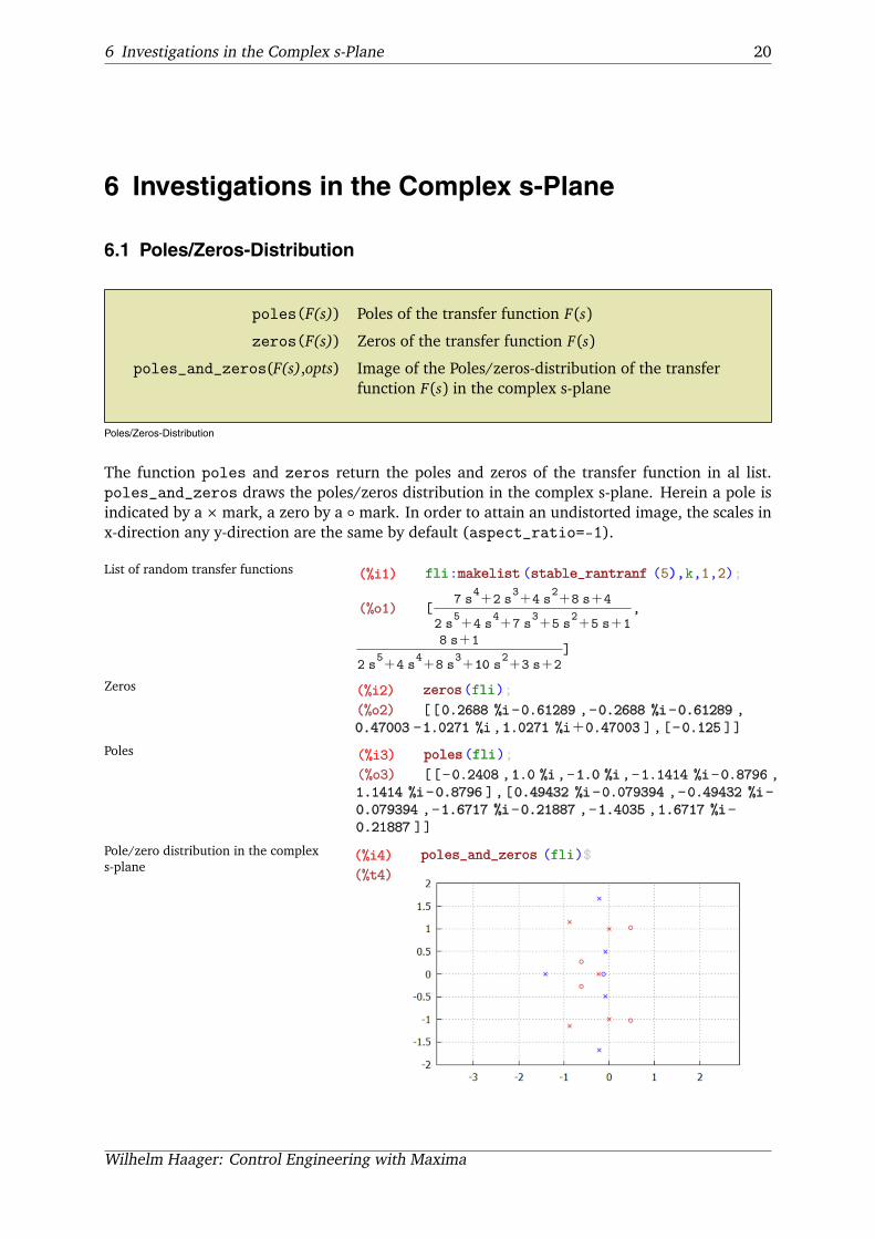
6.1 Poles/Zeros-Distribution

poles(F(s)) Poles of the transfer function F(s)

zeros(F(s)) Zeros of the transfer function F(s)

poles_and_zeros(F(s),opts) Image of the Poles/zeros-distribution of the transferfunction F(s) in the complex s-plane

Poles/Zeros-Distribution

The function poles and zeros return the poles and zeros of the transfer function in al list.poles_and_zeros draws the poles/zeros distribution in the complex s-plane. Herein a pole isindicated by a × mark, a zero by a ◦ mark. In order to attain an undistorted image, the scales inx-direction any y-direction are the same by default (aspect_ratio=-1).

List of random transfer functions (%i1) fli:makelist (stable_rantranf (5),k,1,2);

(%o1) [7 s

4�2 s

3�4 s

2�8 s�4

2 s5�4 s

4�7 s

3�5 s

2�5 s�1

,

8 s�1

2 s5�4 s

4�8 s

3�10 s

2�3 s�2

]

Zeros (%i2) zeros(fli);

(%o2) [[0.2688 %i−0.61289 ,−0.2688 %i−0.61289 ,

0.47003 −1.0271 %i,1.0271 %i�0.47003 ],[−0.125 ]]

Poles (%i3) poles(fli);

(%o3) [[−0.2408 ,1.0 %i,−1.0 %i,−1.1414 %i−0.8796 ,1.1414 %i−0.8796 ],[0.49432 %i−0.079394 ,−0.49432 %i−0.079394 ,−1.6717 %i−0.21887 ,−1.4035 ,1.6717 %i−0.21887 ]]

Pole/zero distribution in the complexs-plane

(%i4) poles_and_zeros (fli)$

(%t4)



6.2 Root Locus Plots

root_locus(F(s,k),opts) Root locus plot of a transfer function F(s, k) with onefree parameter k in the s-plane

trange=[min,max] Range for the free parameter k, default: [0.001,100]

nticks=n Number of calculated points, default: 500

Root locus plots

root_locus draws the root locus of a transfer function F(s) in dependence of a parameter k,which need not be (unlike in “classical” root loci) the open loop gain, but can be an arbitraryparameter influencing the transfer function. If several transfer functions are given in a list, thenames of the parameters can be different, nervertheless their ranges have to be the same for alltransfer functions, determinded by the option trange.

The plot points are distributed over the parameter range logarithmically, thus only positivevalues for the range are allowed.

The starting points of the root loci are indicated by a × mark, the endpoints are indicated by a ◦mark. If the free parameter is the open loop gain, its starting value is sufficiently small, its endvalue is sufficiently large, starting and ending points represent the poles and zeros of the openloop transfer function respectively.

List of transfer functions with variouszeros a and a variating gain k

(%i5) fli:closed_loop (makelist (k*((s-a)*(s+1)) /(s*(s-2)*(s+7)),a,-11,-8));

(%o5) [k s

2�12 k s�11 k

s3�k s

2�5 s

2�12 k s−14 s�11 k

,

k s2�11 k s�10 k

s3�k s

2�5 s

2�11 k s−14 s�10 k

,

k s2�10 k s�9 k

s3�k s

2�5 s

2�10 k s−14 s�9 k

,

k s2�9 k s�8 k

s3�k s

2�5 s

2�9 k s−14 s�8 k

]

Root locus plots in dependence on theopen loop gain k with various values ofthe open loop zero a

(%i6) root_locus (fli,xrange=[-17,3], yrange=[-6,6],nticks=5000)$

(%t6)



Root locus plot of a PT2-element withthe damping ratio as parameter

(%i7) root_locus (1/(s**2+a*s+1),xrange=[-4,1], trange=[1e-4,3],nticks=5000)$

(%t7)


7 Stability Behavior 23

7 Stability Behavior

7.1 Stability

stablep(F(s)) Checks the stability of the system with the der transferfunction F(s)

stability_limit(F(s), k) Calculation of the stability limit of the transfer functionF(s, k) with respect to the parameter k

hurwitz(p(s)) Calculation of the Hurwitz-determinants of thepolynomial p(s)

stable_area(F(s, a, b), a, b, opts)Plot of the stability limit of the transfer functionF(s, a, b) in the a/b-parameter plane

Stability

The function stability_limit(F(s), k) yields conditions for imaginary poles in the form

k = value, ω= value,

which is equivalent to the stability limit for common systems. Herein the value of ω is theangular frequency of the undamped oscillaion at the stability limit. Those conditions can befulfilled also for more than one value of ω. Which condition in fact corresponds to the stabilitylimit, has to be checked by further considerations.Exact conditions for stability are provided by the Hurwitz-criterion: All zeros of the polyno-mial p(s) have a negative realpart (i. e. in exactly that case the transfer function with the de-nominator p(s) is stable), if all Hurwitz determinants have a value greater zero. The functionhurwitz(p(s)) yields a list of the Hurwitz determinants, the coefficients of p(s) can have sym-bolic values.stable_area plots the stability limit of a transfer function with respect to two parameters aand b in the a/b-parameter plane. Unless the options xrange and yrange are given explicitely,the axes range from 0 to 1.

Random transfer function (%i1) f:stable_rantranf (5);

(%o1) 9

s5�3 s

4�9 s

3�10 s

2�7 s�6

Calculation of the closed loop transferfunction with a controller gain of k

(%i2) fw:closed_loop (k*f);

(%o2) 9 k

s5�3 s

4�9 s

3�10 s

2�7 s�9 k�6

Calculation of the stability limit; theresult can be more tan one condition forimaginary poles.

(%i3) lim:stability_limit (fw,k),numer;

(%o3) [[k�−13.709 ,��2.8531 ],[k�0.042326 ,��

0.92733 ]]



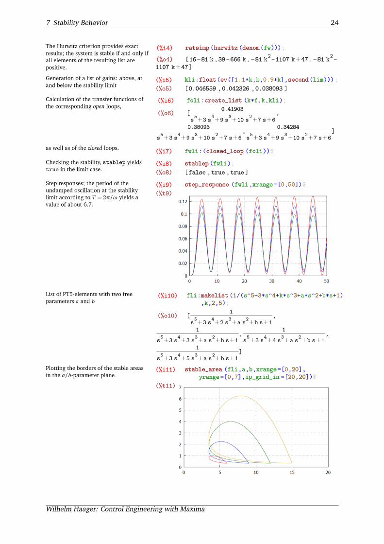
The Hurwitz criterion provides exactresults; the system is stable if and only ifall elements of the resulting list arepositive.

(%i4) ratsimp (hurwitz (denom(fw)));

(%o4) [16−81 k,39−666 k,−81 k2−1107 k�47,−81 k

2−

1107 k�47]

Generation of a list of gains: above, atand below the stability limit

(%i5) kli:float(ev([1.1*k,k,0.9*k],second(lim)));

(%o5) [0.046559 ,0.042326 ,0.038093 ]

Calculation of the transfer functions ofthe corresponding open loops,

(%i6) foli:create_list (k*f,k,kli);

(%o6) [0.41903

s5�3 s

4�9 s

3�10 s

2�7 s�6

,

0.38093

s5�3 s

4�9 s

3�10 s

2�7 s�6

,0.34284

s5�3 s

4�9 s

3�10 s

2�7 s�6

]

as well as of the closed loops.(%i7) fwli:(closed_loop (foli))$

Checking the stability, stablep yieldstrue in the limit case.

(%i8) stablep (fwli);

(%o8) [false ,true ,true ]

Step responses; the period of theundamped oscillation at the stabilitylimit according to T = 2π/ω yields avalue of about 6.7.

(%i9) step_response (fwli,xrange=[0,50])$

(%t9)

List of PT5-elements with two freeparameters a and b

(%i10) fli:makelist (1/(s^5+3*s^4+k*s^3+a*s^2+b*s+1)

,k,2,5);

(%o10) [1

s5�3 s

4�2 s

3�a s

2�b s�1

,

1

s5�3 s

4�3 s

3�a s

2�b s�1

,1

s5�3 s

4�4 s

3�a s

2�b s�1

,

1

s5�3 s

4�5 s

3�a s

2�b s�1

]

Plotting the borders of the stable areasin the a/b-parameter plane

(%i11) stable_area (fli,a,b,xrange=[0,20], yrange=[0,7],ip_grid_in =[20,20])$

(%t11)



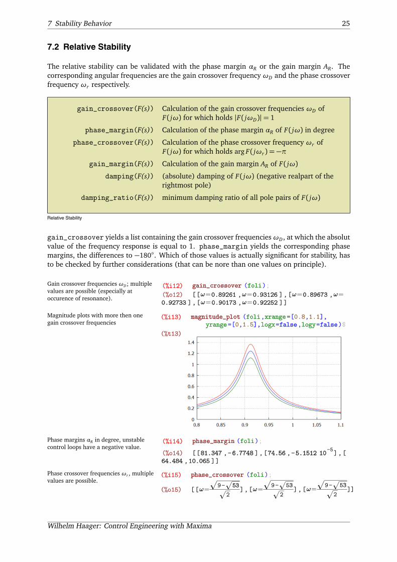
7.2 Relative Stability

The relative stability can be validated with the phase margin αR or the gain margin AR. Thecorresponding angular frequencies are the gain crossover frequency ωD and the phase crossoverfrequency ωr respectively.

gain_crossover(F(s)) Calculation of the gain crossover frequencies ωD ofF( jω) for which holds |F( jωD)|= 1

phase_margin(F(s)) Calculation of the phase margin αR of F( jω) in degree

phase_crossover(F(s)) Calculation of the phase crossover frequency ωr ofF( jω) for which holds arg F( jωr) = −π

gain_margin(F(s)) Calculation of the gain margin AR of F( jω)

damping(F(s)) (absolute) damping of F( jω) (negative realpart of therightmost pole)

damping_ratio(F(s)) minimum damping ratio of all pole pairs of F( jω)

Relative Stability

gain_crossover yields a list containing the gain crossover frequenciesωD, at which the absolutvalue of the frequency response is equal to 1. phase_margin yields the corresponding phasemargins, the differences to −180◦. Which of those values is actually significant for stability, hasto be checked by further considerations (that can be nore than one values on principle).

Gain crossover frequencies ωD; multiplevalues are possible (especially atoccurence of resonance).

(%i12) gain_crossover (foli);

(%o12) [[��0.89261 ,��0.93126 ],[��0.89673 ,��

0.92733 ],[��0.90173 ,��0.92252 ]]

Magnitude plots with more then onegain crossover frequencies

(%i13) magnitude_plot (foli,xrange=[0.8,1.1], yrange=[0,1.5],logx=false,logy=false)$

(%t13)

Phase margins αR in degree, unstablecontrol loops have a negative value.

(%i14) phase_margin (foli);

(%o14) [[81.347 ,−6.7748 ],[74.56 ,−5.1512 10−5],[

64.484 ,10.065 ]]

Phase crossover frequencies ωr , multiplevalues are possible.

(%i15) phase_crossover (foli);

(%o15) [[��

9−

53

2],[��

9−

53

2],[��

9−

53

2]]



Gain margins AR, unstable control loopshave a value less than 1.

(%i16) gain_margin (foli);

(%o16) [[0.90909 ],[1.0 ],[1.1111 ]]

damping calculates the damping σ of a transfer function. That is the negative realpart of theoutmost right pole or pole pair. It indicates the speed of decaying (or stoking up) of a transientprocess. The damping ratio D is the relative damping, related to the natural angular frequencyωn of a pole pair. damping_ratio calculates the minimum damping ratio of all pole pairs of atransfer function. Stable transfer functions have positive values of σ and D, unstable transferfunctions have negative values

Damping of three transfer functions (%i17) damping (fwli);

(%o17) [−0.0020036 ,0,0.0020153 ]

Damping ratio of three transfer functions (%i18) damping_ratio (fwli);

(%o18) [−0.0021573 ,0.0 ,0.0021766 ]


8 Optimization 27

8 Optimization

The performance index according to the ISE-criterion can be calculated according to Parseval’stheorem directly in the Laplace domain:

IISE =

∫ ∞

0

e2(t)dt =1

2π j

∫ j∞

− j∞E(s) · E(−s)ds

Herein e(t) is a function tending to zero with increasing time, usually the deviation of thecontrolled variable from its stationary value. According to [6] the integral can be calculatedalgebraically.

ise(E(s)) Performance index of the function e(t) according to theISE-criterion

Integral performance indexes

Differentiation of the integral with respect to the free parameters (e. g. the controller parame-ters) and setting the results zo zero yield the optimum values of the parameters.

transfer function with two freeparameters a and b

(%i1) f:1/(s**3+a*s**2+b*s+1);

(%o1) 1

s3�a s

2�b s�1

Calculation of the deviation from thestationary value at input step function

(%i2) xs:ratsimp ((1-f)/s);

(%o2) s2�a s�b

s3�a s

2�b s�1

Preformance index according to theISE-criterion

(%i3) iise:ise(xs);

(%o3) a b

2−b�a

2

2 a b−2

Differentiation with respect to theparameters a and b (Calculation of theJacobian matrix)

(%i4) abl:ratsimp (jacobian ([iise],[a,b]));

(%o4) a2b−2 a

2 a2b2−4 a b�2

a2b2−2 a b−a

3�1

2 a2b2−4 a b�2

Confinement to real solutions of systemsof equations

(%i5) realonly :true;

(%o5) true

Solving the equations with respect to aand b, the expressions are assumed to beset to zero.

(%i6) res:solve(abl[1],[a,b]);

(%o6) [[a�1,b�2]]

Substituting the solutions into f yieldsthe “optimum” transfer function.

(%i7) fopt:ev(f,res);

(%o7) 1

s3�s

2�2 s�1



9 Controller Design

gain_optimum(Fs(s),Fr(s)) Calculation of a controller according to the gainoptimum.

Controller Design

gain_optimum calculates the parameters of an optimum controller FR(s) for a given plant F(s).The strucuture of the controller and the names of its parameters are freely chooseable on prin-cipal. It depends on the reasonableness of the assumtions for the controller, whether solutionsfor the controller paraneters are found actually (e.g. a PT1-controller will presumeably not yieldsoutions).

Transfer function of a plant (%i1) fs:2/((1+5*s)*(1+s)**2*(1+0.3*s));

(%o1) 2

� �

0.3 s�1� �

s�12 � �

5 s�1

List of an I-, PI- and a PID-controller (%i2) [fri,frpi,frpid]:[1/(s*Ti),kr*(1+1/(s*Tn)),(1+s*Ta)*(1+s*Tb)/(s*Tc)];

(%o2) [1

Ti s,kr

� �

� �1

Tn s�1 ,

� �

Ta s�1� �

Tb s�1

Tc s]

Gain optimum for the I-controller (%i3) g1:gain_optimum (fs,fri);

(%o3) [Ti�146

5,Ti�0]

Gain optimum for the PI-controller; thezero of the controller approximatelycompensates the dominating pole of theplant.

(%i4) g2:gain_optimum (fs,frpi);

(%o4) [kr�206057

349320,Tn�

206057

40190]

Gain optimum for the PID-controllerr;the zeros of the controller approximatelycompensate the two dominating poles ofthe plant.

(%i5) g3:float(gain_optimum (fs,frpid));

(%o5) [Tc�3.6197 ,Ta�4.9984 ,Tb�1.3966 ]

Substituting the results into thecontrollers

(%i6) reli:float(ev([fri,frpi,frpid],[g1,g2,g3]));

(%o6) [0.034247

s,0.58988

� �

� �0.19504

s�1.0 ,

0.27627� �

1.3966 s�1.0� �

4.9984 s�1.0

s]



The step responses confirm about 5%overshoot and rise times in the amountof about 4.7 times the sum of theremaining time constants.

(%i7) step_response (float(ev(closed_loop (reli*fs), res)),yrange=[0,1.5])$

(%t7)

The plant can also have symboliccoefficients.

(%i8) fs:2/((1+a*s)*(1+s**2)*(1+b*s));

(%o8) 2

� �

a s�1� �

b s�1

� �

s2�1

The results are formulas for theoptimum controller parameters.

(%i9) gain_optimum (fs,frpi);

(%o9) [kr�b2�a

2−1

4 a b,Tn�

b3�a b

2�

� �

a2−1 b�a

3−a

b2�a b�a

2−1

]


10 State Space 30

10 State Space

System: [A, B, C, D] Definition of a linear system as a list of state matrices A,B, C und D

systemp(A, B, C [, D])systemp(system) Checks, whether system is a valid system constiting of

state matrices.

nsystemp(A, B, C [, D])nsystemp(system) Cecks, whether system forms a valid linear system,

wherein all matrix elements evaluate to numbers.

transfer_function(A, B, C [, D])transfer_function(System) Calculation of the transfer function (or transfer matrix)

from the state matrices

controller_canonical_form(f)Calculation of the state matrices according to thecontroller canonical from the transfer function f

observer_canonical_form(f)Calculation of the state matrices according to theobserver canonical from the transfer function f

controllability_matrix(A, B)controllability_matrix(System)

Calculation of the controllability matrix

observability_matrix(A, C)observability_matrix(System)

Calculation of the observability matrix

State space representation

The notion system means a subsumption of the four state matrices A (system matrix), B (inputmatrix), C (output matrix) and D (transit matrix) into a list. The transit matrix D can be omittedfor systems without feedthrough, for systems with one input and one output D can be a scalarvalue d.

All funcions, which can have a system as the parameter, can also receive the particular statematrices as parameters (without subsumption into a list).


10 State Space 31

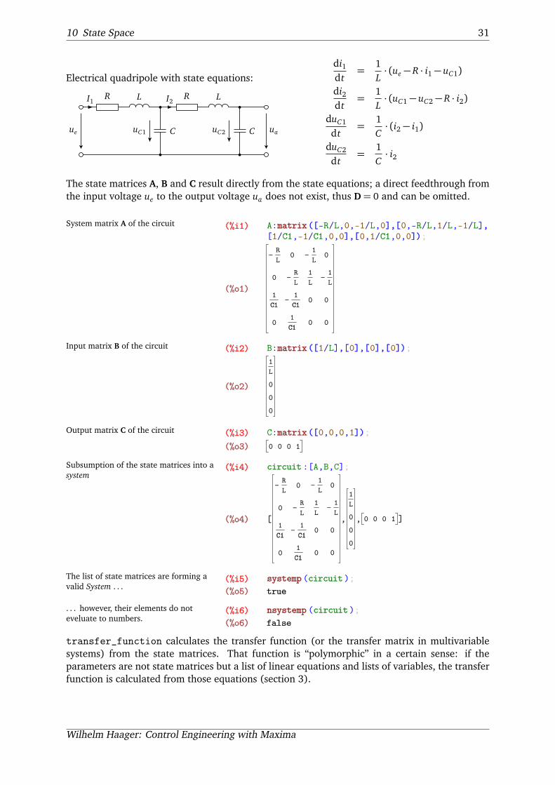
Electrical quadripole with state equations:

R L R L

C Cue uauC1 uC2

I1 I2

di1dt

=1L· (ue − R · i1 − uC1)

di2dt

=1L· (uC1 − uC2 − R · i2)

duC1

dt=

1C· (i2 − i1)

duC2

dt=

1C· i2

The state matrices A, B and C result directly from the state equations; a direct feedthrough fromthe input voltage ue to the output voltage ua does not exist, thus D= 0 and can be omitted.

System matrix A of the circuit (%i1) A:matrix([-R/L,0,-1/L,0],[0,-R/L,1/L,-1/L],

[1/C1,-1/C1,0,0],[0,1/C1,0,0]);

(%o1)

−R

L

0

1

C1

0

0

−R

L

−1

C1

1

C1

−1

L

1

L

0

0

0

−1

L

0

0

Input matrix B of the circuit (%i2) B:matrix([1/L],[0],[0],[0]);

(%o2)

1

L

0

0

0

Output matrix C of the circuit (%i3) C:matrix([0,0,0,1]);

(%o3) 0 0 0 1

Subsumption of the state matrices into asystem

(%i4) circuit :[A,B,C];

(%o4) [

−R

L

0

1

C1

0

0

−R

L

−1

C1

1

C1

−1

L

1

L

0

0

0

−1

L

0

0

,

1

L

0

0

0

, 0 0 0 1 ]

The list of state matrices are forming avalid System . . .

(%i5) systemp (circuit );

(%o5) true

. . . however, their elements do noteveluate to numbers.

(%i6) nsystemp (circuit );

(%o6) false

transfer_function calculates the transfer function (or the transfer matrix in multivariablesystems) from the state matrices. That function is “polymorphic” in a certain sense: if theparameters are not state matrices but a list of linear equations and lists of variables, the transferfunction is calculated from those equations (section 3).


10 State Space 32

Calculation of the transfer function;providing a system, . . .

(%i7) f:transfer_function (circuit );

(%o7) 1

C12L2s4�2 C1

2L R s

3�C1

2R2s2�3 C1 L s

2�3 C1 R s�1

. . . as well as particular state matrices ispossible.

(%i8) transfer_function (A,B,C);

(%o8) 1

C12L2s4�2 C1

2L R s

3�C1

2R2s2�3 C1 L s

2�3 C1 R s�1

Direct calculation of an impedance chainyields the same result expectedly.

(%i9) f:impedance_chain (R+s*L,1/(s*C1),2);

(%o9) 1

C12L2s4�2 C1

2L R s

3�

� �

C12R2�3 C1 L s

2�3 C1 R s�1

The state matrices can be calculated from the transfer function according to the controller canon-ical form or the observer canonical form:

Controller canonical form of the statematrices

(%i10) circ1:controller_canonical_form (f);

(%o10) [

0

0

0

−1

C12L2

1

0

0

−3 R

C1 L2

0

1

0

−C1

2R2�3 C1 L

C12L2

0

0

1

−2 R

L

,

0

0

0

1

,1

C12L2

0 0 0

0]

Observer canonivcal foem of the statematrices

(%i11) circ2:observer_canonical_form (f);

(%o11) [

0

1

0

0

0

0

1

0

0

0

0

1

−1

C12L2

−3 R

C1 L2

−C1

2R2�3 C1 L

C12L2

−2 R

L

,

1

C12L2

0

0

0

, 0 0 0 1 ,0]

Controllability matrix (%i12) h1:ratsimp (controllability_matrix (A,B));

(%o12)

1

L

0

0

0

−R

L2

0

1

C1 L

0

C1 R2−L

C1 L3

1

C1 L2

−R

C1 L2

0

−C1 R

3−2 L R

C1 L4

−2 R

C1 L3

C1 R2−2 L

C12L3

1

C12L2


10 State Space 33

Observability matrix (%i13) h2:observability_matrix (circuit );

(%o13)

0

0

0

1

C12L

0

1

C1

−R

C1 L

R2

C1 L2−

2

C12L

0

0

1

C1 L

−R

C1 L2

1

0

−1

C1 L

R

C1 L2

The system is controllable andobservable.

(%i14) [rank(h1),rank(h2)];

(%o14) [4,4]


11 Various Functions 34

11 Various Functions

The package COMA provides several auxiliary functions which are not specific to control engi-neering, but can be useful in various calculations.

R1 // R2 Parallel connection of two resistors R1 and R2

Z /_ ϕ Polar coordinate representation of a complex numberz = Z∠ϕ (Z „cis“ ϕ)

z cf Postfix-Operator, outputs the complex number z inpolar coordinate representation Z∠ϕ

chop(x) Replaces all numbers in the expression x, which are lessthan 10−10, by 0

coefficient_list(p, x) List of the coefficients of the polynomial p in thevariable x

set_option(name=val, list) Setting or adding an element as a key-value pair to list

delete_option(name, list) Deleting of a key-value pair name from list

option_exists(name, list) Checks, whether a key-value pair name exists in list

list_option_exists(name, list)Checks, whether a key-value pair with the name nameexists in list and its value is a list itself

Various functions

„//“ and „/_“ are two operators common in electrical enigneering: for the parallel connectionof resistors and for complex quantities in polar coordinate representation. The postfix operatorcf outputs a complex quantity in polar coordinates.

Parallel connection of impedances (%i1) R // 1/(s*C) // s*L + R1;

(%o1) L R s

C L R s2�L s�R

�R1

Polar coordinate represenation ofcomplex quantities

(%i2) [U1,U2,U3]:[230,230/_240,230/_120];

(%o2) [230 ,−199.19 %i−115.0 ,199.19 %i−115.0 ]

Output of a complex quantity in polarcoordinates

(%i3) U1+U3 cf;

(%o3) 230.0 /_ 60.0

coefficient_list builds a list of the polynomial coefficients in increasing order:

Polynomial in the variable x (%i4) p:5*(x+y)^2+a*x^5;

(%o4) 5� �

y�x2�a x

5


Bibliography 35

List containing the polynomialcoefficients

(%i5) coefficient_list (p,x);

(%o5) [5 y2,10 y,5,0,0,a]

The function chop removes all numbers from an expression, which are less than 10−10. That isuseful for “ironing out” numeric bugs:

When the numeric fails, . . . (%i6) x3:expand((s^2-1.1*s+1.1) *(s^2+1.1*s+1.1)*(s^2+1));

(%o6) s6�1.99 s

4�2.2204 10

−16s3�2.2 s

2�1.21

. . . erroneously emerging small numberscan be removed.

(%i7) chop(x3);

(%o7) s6�1.99 s

4�2.2 s

2�1.21

An associative array (hash), consisting of key-value pairs, is implemented as a list. It is wellsuited for saving preferences (“options”) and for named parameters of functions (e. g. graphicroutines).

Some routines facilitate the handling of associative arrays:

List of key-value pairs (%i8) opts:[color=blue,xrange=[0,10]];

(%o8) [color�blue ,xrange�[0,10]]

Replacing a value (%i9) set_option (color=red,opts);

(%o9) [xrange�[0,10],color�red ]

Unless a key exists, a new key-value pairis generated.

(%i10) set_option (title="Test",opts);

(%o10) [xrange�[0,10],color�red ,title�Test ]

Removing a key-value pair (%i11) delete_option (color,opts);

(%o11) [xrange�[0,10],title�Test ]

Checking, whether a key exists (%i12) option_exists (xrange,opts);

(%o12) true

Reading a hash value (%i13) get_option (title,opts);

(%o13) Test

Returning a default value, unless a keyexists

(%i14) get_option (color,opts,red);

(%o14) red

The function get_option to read out a value would not be not neccessary on principal, for thatpurpose the Maxima function assoc is available. Contrary to assoc, get_option accepts alsolists, which not only contain key-value pairs, but also any arbitrary expression (which is usedinternally by other by other COMA-functions).


Bibliography 36

Bibliography

[1] Maxima Development Team: Maxima Manual Version 5.39.0,http://maxima.sourceforge.net 2016 .

[2] Various Authors: Gnuplot 4.6, An Interactive Plotting Program,http://www.gnuplot.info 2014 .

[3] Rodríguez Riotorto, M.: A Maxima-Gnuplot Interface,http://riotorto.users.sourceforge.net/Maxima/gnuplot/index.html.

[4] Haager W.: Computeralgebra mit Maxima, Hanser München, Leipzig 2014.

[5] Haager W.: Regelungstechnik kompetenzorientiert, Hölder Pichler Tempsky Wien 2016.

[6] Newton G., Gould L., Kaiser J.: Analytical Design of Linear Feedback Control, Wiley, NewYork 1957.


Documents

COMA Control Engineering with Maxima - Austromath · Control Engineering with Maxima Wilhelm Haager ... is passed to Gnuplot via the option user_preamble in appropriate form