Embed Size (px)
Citation preview
Column generation based approaches for a tour
scheduling problem with a multi-skill heterogeneous
workforce
Matthieu Gerarda, Francois Clautiauxb,∗, Ruslan Sadykovb
aCompany ASYS Paris, Inria Lille - Nord Europe, Universite de Lille 1bInstitut de Mathematiques de Bordeaux (UMR CNRS 5251), Universite de Bordeaux,
Inria Bordeaux - Sud Ouest
Abstract
In this paper, we address a multi-activity tour scheduling problem with timevarying demand. The objective is to compute a team schedule for a fixedroster of employees in order to minimize the over-coverage and the under-coverage of different parallel activity demands along a planning horizon ofone week. Numerous complicating constraints are present in our problem:all employees are different and can perform several different activities duringthe same day-shift, lunch breaks and pauses are flexible, demand is givenfor 15 minutes periods. Employees have feasibility and legality rules to besatisfied, but the objective function does not account for any quality mea-sure associated with each individual’s schedule. More precisely, the problemmixes simultaneously days-off scheduling, shift scheduling, shift assignment,activity assignment, pause and lunch break assignment.
To solve this problem, we developed four methods: a compact MixedInteger Linear Programming model, a branch-and-price like approach witha nested dynamic program to solve heuristically the subproblems, a divingheuristic and a greedy heuristic based on our subproblem solver. The com-putational results, based on both real cases and instances derived from realcases, demonstrate that our methods are able to provide good quality so-lutions in a short computing time. Our algorithms are now embedded in acommercial software, which is already in use in a mini-mart company.
∗Corresponding Author. Institut de Mathematiques de Bordeaux, Universite de Bor-deaux, 351, cours de la Liberation - F 33 405 Talence, France
Email address: [email protected] (Francois Clautiaux)
Preprint submitted to European Journal of Operational Research December 10, 2015
Keywords: employee scheduling, integer programming, branch-and-price,heuristics
1. Introduction
Employee scheduling is an important issue in retail (see [1]), as person-nel wages account for a large part of their operational costs. This problemraises considerable computational difficulties, especially when certain fac-tors are considered, such as employee availability, fairness, strict labor rules,highly variable work demand, mixed full and part-time contracts, etc. Sincethe seminal work of Dantzig [2], a large quantity of research papers havedeveloped models and methods to assist managers and planners in their em-ployee scheduling tasks (more than 300 papers published between 2004 and2012 were surveyed in [3]). For a comprehensive literature review of classicalstudies on this problem, we refer to [4].
In this paper, we study a real-life multi-activity tour scheduling problemwith highly heterogeneous employees and flexible working hours. Given afixed set of employees, the objective is to construct their work schedule orplanning that minimizes the distance to the ideal coverage of the demand.Numerous complicating factors described in the literature are taken into ac-count and, to the best of our knowledge, this paper is one of the first attempts(in parallel with [5]) to combine days-off scheduling, shift scheduling, shiftassignment, activity assignment, pause and lunch break assignment.
Several features of our problem are still considered as major issues inthe recent literature [3]: individual constraints and flexibility of employees,integrated days-off, shift scheduling and assignment [6] and multi-activity as-signment [7, 8, 9]. Although the lunch break assignment between two times-lots is taken into account in most research papers, pause assignment duringactivities themselves remains a gap in the academic literature (see [10]). Toour knowledge, only [11] deals with both types of breaks at the same time.
Although integer linear programming (ILP) models exist for this familyof problems, they cannot be used directly to solve large scale problems withmany constraints. Therefore, several works propose heuristics based on thoseILP models to reduce their computational burden. Heuristic methods canbe obtained by applying a hierarchical decomposition (see e.g. [12]). First,good shifts are computed, and then employees are assigned to the shifts in asecond phase. Unfortunately, this technique cannot be applied directly to ourproblem, where each employee can change activity during his shift and has his
2
very specific features such as availabilities, skills and pre-assignments. Whenthe time horizon is large, and the problem can be solved for a smaller timehorizon (typically one week) without risking infeasibilities for the planning,an interesting approach [13] is to use a rolling horizon heuristic, where theproblems related to smaller time horizons are solved in an iterative manner.In our problem, the total number of worked hours for each employee is fixed,which may lead such method to unfeasible schedules.
Many algorithms for solving such employee scheduling problems are basedon the column-generation approach (see for example [14]). Recent papers ad-dress shift or tour scheduling problems with branch-and-price methods. Coteet al. [15], Boyer et al. [16] and Restrepo et al. [5] use branch-and-price tosolve very general multi-activity shift scheduling problems. Their approachesrely on the description of shifts using a context-free grammar. Another re-cent work on the subject was realized by Brunner and Stolletz [17]. Theyuse an ad-hoc branch-and-price method to solve a tour scheduling problem.The main ingredients of their approach are the use of variables related today-shifts, which are recombined in the master problem, and stabilizationstrategies to reduce the number of column generation iterations. Another re-cent work [18] uses branch-and-price in the context of employee-scheduling.They use a nested dynamic programming approach, which is well-suited tothe structure of their problem.
Our approach is also based on a branch-and-price algorithm. However,the problem settings do not allow us to use directly the algorithms from[15, 16, 5]. In our problem, each employee is different, the time horizonis much larger than the ones in [16, 15], and many constraints restrict theconstruction of the shifts. This leads to a prohibitively large pricing problemsolution time. Since our aim is to handle real-life instances, we had to use aheuristic version of the branch-and-price, where some constraints are treatedheuristically in the subproblem. The hierarchical structure of our shifts calledfor an ad-hoc specific nested dynamic program (like [18]), which proves to bemuch more efficient than a straightforward dynamic programming approach.
An important practical requirement is to find a good solution in a shortamount of time (a few seconds for 100 employees). To respect this timelimit, we designed a greedy algorithm based on our dynamic program. Also,a diving heuristic is proposed for cases when we have several minutes ofcomputational time. Our algorithms have been implemented and are nowembedded in a commercial software. They are able to find feasible solutionswith good quality in a small or reasonable time for all test cases that were
3
provided by our industrial partner. Our algorithms are now in use in a mini-mart company.
In Section 2, we describe formally our problem. Our column generationframework is presented in Section 3, followed by the nested dynamic programused to solve the pricing problem in Section 4. Our heuristic algorithmsbased on column generation are presented in Section 5, while computationalexperiments on real and generated instances are reported in section 6.
2. Problem description
The problem consists in scheduling a fixed workforce to maximize the fit toa given time-varying demand. The planning horizon consists of D consecutivedays. Each day is divided into the same number of successive time periods ofequal length (15 minutes in this paper). Set T represents the different timeperiods in the discrete planning horizon. The set of heterogeneous employeesis denoted by E .
The whole set of activities that employees can carry out is divided intotwo distinct groups: production activities A, related to work demands, andpause activities P , related to non-productive activities. In our retail context,a production activity can represent, for example, the welcome desk, a cashdesks line or a meat counter. Each employee e ∈ E has a set of produc-tion activities A(e, t) that he/she can perform at time period t. Set P(e, t)contains a pause if employee can take it at time period t; this set is emptyotherwise. The beginning and the length of a pause are strictly constrainedby the personalized pause policy of the company agreement. An employeee is unavailable at time period t if A(e, t) ∪ P(e, t) = ∅. In this case, theplanning computed for employee e cannot contain any activity at time t.Note that if an employee is unavailable the entire day, then a day-off has tobe scheduled. Some employees may be pre-assigned to activities for certaintime periods. In this case, finding a schedule that respects this pre-assignedtasks is a part of the problem.
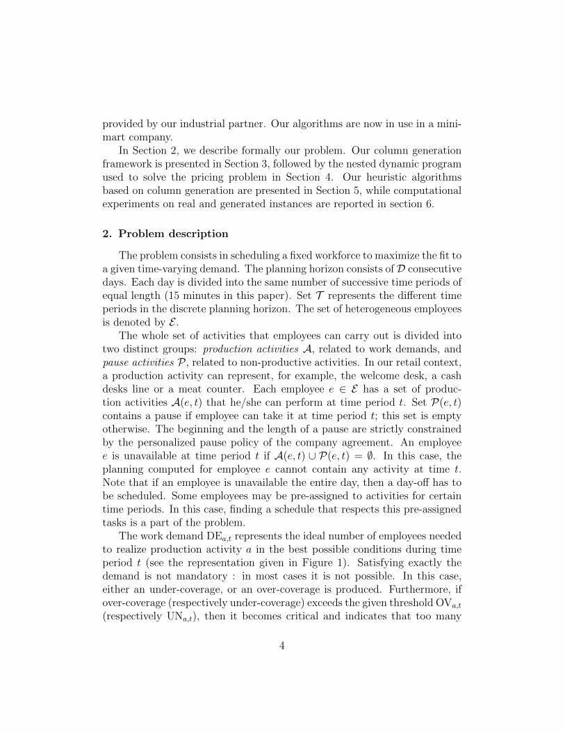
The work demand DEa,t represents the ideal number of employees neededto realize production activity a in the best possible conditions during timeperiod t (see the representation given in Figure 1). Satisfying exactly thedemand is not mandatory : in most cases it is not possible. In this case,either an under-coverage, or an over-coverage is produced. Furthermore, ifover-coverage (respectively under-coverage) exceeds the given threshold OVa,t
(respectively UNa,t), then it becomes critical and indicates that too many
4

t
number ofemployees
Figure 1: representation of the workload for a production activity : the ideal number ofemployees required to cover the demand is in gray, the thresholds of critical undercoverageand overcoverage are given respectively in black and white.
(respectively too few) employees have been assigned to activity a duringtime period t.
Our objective is to construct a feasible team schedule that minimizes thesum of the over-coverage and under-coverage costs for the whole planninghorizon and all production activities.
2.1. A hierarchical structure of a team schedule
A feasible solution follows a hierarchical structure (see Figure 2). Foreach level of the hierarchy, there is an associated set of constraints. Thisflexible structure does not rely on the use of a pre-computed day-shift orindividual planning library, since the number of possibilities is far too large.
team schedule
individualplanning
day-off
day-shift timeslot tasktime
period
Figure 2: Hierarchical structure of a team schedule.
• A team schedule consists of a set of |E| valid employee plannings.
5
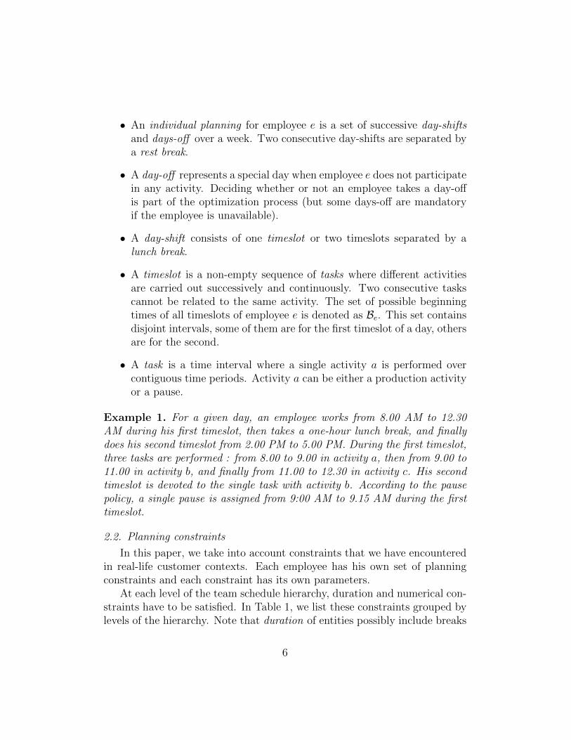
• An individual planning for employee e is a set of successive day-shiftsand days-off over a week. Two consecutive day-shifts are separated bya rest break.
• A day-off represents a special day when employee e does not participatein any activity. Deciding whether or not an employee takes a day-offis part of the optimization process (but some days-off are mandatoryif the employee is unavailable).
• A day-shift consists of one timeslot or two timeslots separated by alunch break.
• A timeslot is a non-empty sequence of tasks where different activitiesare carried out successively and continuously. Two consecutive taskscannot be related to the same activity. The set of possible beginningtimes of all timeslots of employee e is denoted as Be. This set containsdisjoint intervals, some of them are for the first timeslot of a day, othersare for the second.
• A task is a time interval where a single activity a is performed overcontiguous time periods. Activity a can be either a production activityor a pause.
Example 1. For a given day, an employee works from 8.00 AM to 12.30AM during his first timeslot, then takes a one-hour lunch break, and finallydoes his second timeslot from 2.00 PM to 5.00 PM. During the first timeslot,three tasks are performed : from 8.00 to 9.00 in activity a, then from 9.00 to11.00 in activity b, and finally from 11.00 to 12.30 in activity c. His secondtimeslot is devoted to the single task with activity b. According to the pausepolicy, a single pause is assigned from 9:00 AM to 9.15 AM during the firsttimeslot.
2.2. Planning constraints
In this paper, we take into account constraints that we have encounteredin real-life customer contexts. Each employee has his own set of planningconstraints and each constraint has its own parameters.
At each level of the team schedule hierarchy, duration and numerical con-straints have to be satisfied. In Table 1, we list these constraints grouped bylevels of the hierarchy. Note that duration of entities possibly include breaks
6
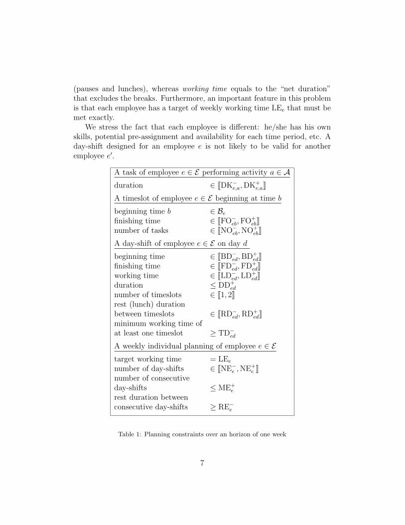
(pauses and lunches), whereas working time equals to the “net duration”that excludes the breaks. Furthermore, an important feature in this problemis that each employee has a target of weekly working time LEe that must bemet exactly.
We stress the fact that each employee is different: he/she has his ownskills, potential pre-assignment and availability for each time period, etc. Aday-shift designed for an employee e is not likely to be valid for anotheremployee e′.
A task of employee e ∈ E performing activity a ∈ Aduration ∈ JDK−e,a,DK+
e,aK
A timeslot of employee e ∈ E beginning at time b
beginning time b ∈ Befinishing time ∈ JFO−eb,FO+
ebKnumber of tasks ∈ JNO−eb,NO+
ebK
A day-shift of employee e ∈ E on day d
beginning time ∈ JBD−ed,BD+edK
finishing time ∈ JFD−ed,FD+edK
working time ∈ JLD−ed,LD+edK
duration ≤ DD+ed
number of timeslots ∈ J1, 2Krest (lunch) durationbetween timeslots ∈ JRD−ed,RD+
edKminimum working time ofat least one timeslot ≥ TD−ed
A weekly individual planning of employee e ∈ Etarget working time = LEe
number of day-shifts ∈ JNE−e ,NE+e K
number of consecutiveday-shifts ≤ ME+
e
rest duration betweenconsecutive day-shifts ≥ RE−e
Table 1: Planning constraints over an horizon of one week
7
2.3. Pause assignment policy
There are numerous pause assignment policies in practice. In this work,we use the following rules. First, pauses are not included in the working time.There is at most one pause assigned per timeslot. The pause is assigned ifand only if the duration of the timeslot is at least four hours (including thepause duration). A pause must be located in the second third of its timeslot,and its duration is exactly one time period. Some pauses can be initially setat some time periods as pre-assignment constraints.
In our settings, each pause is positioned inside an existing task k. Thetwo parts of task k before and after the pause are considered as a uniquetask, i.e. the two constitute a single task with one begining and one end.Note that pauses are different from lunch breaks in our models: a lunch breakseparates the day-shift into two timeslots.
3. Our column generation approach
The Dantzig-Wolfe decomposition [19] is well adapted to our schedulingproblem, since it consists of disjoint subproblems (one per employee) that arelinked by demand constraints. Similarly to [2], the subproblem for employeee consists in designing a valid individual planning respecting the specific setof constraints of employee e, but disregarding the requirements dealing withthe others plannings. The master problem combines the employee plannings(columns) to minimize the total cost of over-coverage and under-coverage.
Another version of the set-covering model for the tour scheduling was pro-posed by Stolletz [20]. Instead of using variables representing plannings, theauthor uses (day-)shift variables that are combined in the master problem toform valid plannings. Our problem settings do not allow easy recombinationsof shifts: all employees are different and therefore each planning is associ-ated to exactly one employee, and the total number of working periods in aplanning is a fixed parameter. In our model, we keep the original planningvariables, similar to what is done in [2].
3.1. Master problem
Let X (e) denote the set of individual plannings (or columns) for employeee and C(e) its column index set: X (e) = Xcc∈C(e). Each column Xc isrepresented by a vector [xc,a,t]t∈T ,a∈A where:
8
ObjectiveValue
under-coverage over-coverage
OVa,tUNa,t
ova,t ovcrita,tuna,tuncrita,t
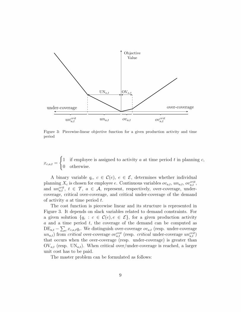
Figure 3: Piecewise-linear objective function for a given production activity and timeperiod
xc,a,t =
1 if employee is assigned to activity a at time period t in planning c,
0 otherwise.
A binary variable qc, c ∈ C(e), e ∈ E , determines whether individualplanning Xc is chosen for employee e. Continuous variables ova,t, una,t, ov
crita,t ,
and uncrita,t , t ∈ T , a ∈ A, represent, respectively, over-coverage, under-coverage, critical over-coverage, and critical under-coverage of the demandof activity a at time period t.
The cost function is piecewise linear and its structure is represented inFigure 3. It depends on slack variables related to demand constraints. Fora given solution qc : c ∈ C(e), e ∈ E, for a given production activitya and a time period t, the coverage of the demand can be computed asDEa,t −
∑c xc,a,tqc. We distinguish over-coverage ova,t (resp. under-coverage
una,t) from critical over-coverage ovcrita,t (resp. critical under-coverage uncrita,t )that occurs when the over-coverage (resp. under-coverage) is greater thanOVa,t (resp. UNa,t). When critical over/under-coverage is reached, a largerunit cost has to be paid.
The master problem can be formulated as follows:
9

min∑a∈A
∑t∈T
COa · ova,t + COcrita · ovcrit
a,t + CUa · una,t + CUcrita · uncrit
a,t (1)
s.t.∑e∈E
∑c∈C(e)
xc,a,t qc − (ova,t + ovcrita,t ) + (una,t + uncrit
a,t ) = DEa,t
∀t ∈ T ,∀a ∈ A(2)
∑c∈C(e)
qc = 1 ∀e ∈ E (3)
una,t ≤ UNa,t, ∀t ∈ T ,∀a ∈ A (4)
ova,t ≤ OVa,t, ∀t ∈ T ,∀a ∈ A (5)
qc ∈ 0, 1 ∀e ∈ E ,∀c ∈ C(e) (6)
una,t, ova,t ∈ R+ ∀t ∈ T ,∀a ∈ A (7)
uncrita,t , ov
crita,t ∈ R+ ∀t ∈ T ,∀a ∈ A (8)
The piecewise objective function (1) minimizes the total cost of over-coverage and under-coverage over the planning horizon and production ac-tivities. Constant values COa ∈ R+ and CUa ∈ R+ represent, respectively,the unitary costs of over-coverage and under-coverage for production activ-ity a. Constant values COcrit
a ∈ R+ and CUcrita ∈ R+ represent respectively
the costs of critical over-coverage and under-coverage for production activ-ity a. Critical over-coverage and critical under-coverage have larger costs:CUa < CUcrit
a and COa < COcrita .
Constraints (2) link the decision variables and calculate the gap betweenthe produced work and the work demand DEa,t for each time period and eachproduction activity. Constraints (3) assign exactly one individual planningto each employee e.
3.2. Pricing subproblems
The pricing problem decomposes into |E| independent subproblems (onefor each employee). Let [πa,t]t∈T ,a∈A be the dual values related to masterproblem constraints (2) and [πe]e∈E be the dual values related to masterproblem constraints (3). The subproblem for employee e consists in finding
10
a feasible individual planning (denoted by vector X = [xa,t]t∈T ,a∈A) with theminimum reduced cost. We use variables xa,t, which will be used to constructthe constant column descriptors xc,a,t in the master problem. Recall thatX (e) denotes the set of individual planning (or columns) for employee e.The subproblem for employee e can be stated as follows.
min −πe −∑t∈T
∑a∈A(e,t)
πa,t xa,t (9)
s.t. X ∈ X (e) (10)
3.3. Acceleration strategies
Acceleration techniques are key elements for the efficiency of our columngeneration approach. Several papers list strategies for this purpose (see e.g[21]), and more specifically for employee scheduling problems in [17] and [22].We used the following strategies.
1. Instead of adding one column with the best reduced cost, we add tothe restricted master problem several negative reduced cost columnsat each iteration. Practically speaking, at each ieration of the columngeneration method, we add the best column found for each employeeif it has a negative reduced cost. This means that at most |E| columnsare added at each iteration. This method dramatically decreases thenumber of column generation iterations.
2. After solving a restricted master problem, if the number of variablesexceeds a given threshold (more than 5000 columns in practice), thenwe delete all variables with a reduced cost exceeding 10−12.
3. The lagrangian lower bound is computed at each iteration to stop thealgorithm earlier if this bound and the solution value of the restrictedmaster are equal. The lagrangian lower bound is computed as follows.Let OPT (RMP ) be the optimum of the current reduced master prob-lem and RC(SPe) be the best reduced cost of a variable generated bysubproblem e at the current iteration. The lagrangian lower bound isequal to OPT (RMP )−
∑e∈E RC(SPe).
We have also tried to apply dual price smoothing stabilization [23] inorder to accelerate column generation. However, it did not have a clear posi-tive impact on the solution time. Note that [17] reports very good speed-ups
11
from stabilized column generation in a branch-and-price algorithm for a sim-ilar shift scheduling problem. We conjecture that the explanation for thisdifferent stabilization impact comes from the presence of the total work-ing time constraint in our variant of the problem. Preliminary experimentsshowed that the dual price smoothing stabilization improves a lot the columngeneration solution time once this constraint is removed.
We also tried to solve only one pricing subproblem at each step (by con-sidering only one employee), or to add only the column of best reduced costamong all subproblems. In both cases, the method was less efficient. Thiscan be explained by the fact that solving the master problem takes a largeamount of time. Moreover, several subproblems are solved in parallel, whichhelps reducing the time spent to solve all subproblems.
4. A nested dynamic program for the pricing subproblem
A pricing subproblem corresponds to finding the best individual planningfor one employee according to his set of constraints. In this section, we discusstwo possible ways from the literature to formulate this problem. Then wepresent our nested dynamic programming algorithm.
4.1. Limits of the resource constrained shortest path formulation
The pricing subproblem can be formulated as a resource-constrained short-est path problem (RCSPP) in a directed acyclic graph (DAG). In this DAG,each arc is characterized by a cost to use it and a set of resource consump-tions while each node is characterized by a position in time and an amount ofresource consumption already used for each resource. The objective is to finda path from a source node to a sink node that minimizes the overall cost andsatisfies the resource consumption bounds. In [24], the authors present anexact dynamic programming algorithm based on relaxations and alternatedforward and backward searches to solve shortest path problems involvinga huge number of local resource constraints. This algorithm is much moreefficient when only upper bounds are considered. When both lower and up-per bounds co-exist, the dominance relations, used to reduce enumeration,are weaker. Another recent work [25] propose an exact method capable ofhandling large-scale networks in a reasonable amount of time.
In our problem, we have a large number of lower and upper bounds for theresource consumption, and some arc costs are negative. This weakens con-siderably the dominance rules used in the solution methods for the resource-
12
constraint shortest path problem. Preliminary experiments confirmed thatthis approach was not efficient for our problem.
4.2. Limits of the grammar-based formulation
The structure of individual plannings makes the subproblem suitable fora solution method that uses context-free grammars, like it is done in [15, 16]for a shift scheduling problem (horizon with a single day) and in [5] for a tourscheduling problem (horizon of 7 days). Namely, for each employee e ∈ Ewe can define a grammar which describes the set of all valid plannings fore. Based on this grammar, a directed acyclic hyper-graph (called graph withor-nodes and and-nodes in [16]) can be constructed. Every unit flow in thishyper-graph defines a feasible individual planning for e. So the search for anindividual planning with the best reduced cost can be done using a dynamicprogramming algorithm that seeks a min cost unit flow in the hyper-graph.
We have performed preliminary experiments with this approach and ob-tained the following results. A considerable number of bound constraints(presented in Table 1) and a long time horizon result in a huge hyper-graph.Therefore, the construction of this hyper-graph takes a large amount of time,making it impossible to embed the grammar-based dynamic program in a fastheuristic. Moreover, even if the graph is constructed, this algorithm takestoo much time to be called at every column generation iteration to solve thesubproblem.
Therefore, we designed a nested dynamic programming algorithm. Inorder to reduce its running time, we heuristically remove some states, as itis explained below.
4.3. A nested dynamic programming algorithm
The specific structure of our problem leads to the following observations.
• There are a large number of resource constraints, but only a subset ofthem are active at a given node.
• Many paths share identical subpaths. Due to the hierarchical structureof the planning, the best day-shift for a given day is likely to be usedin many non-dominated partial solutions.
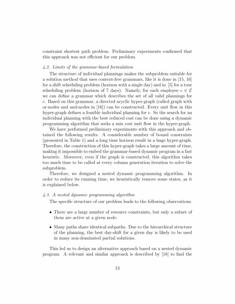
This led us to design an alternative approach based on a nested dynamicprogram. A relevant and similar approach is described by [18] to find the
13

individualplanning
day-off
day-shift timeslot tasktime
period
Figure 4: Nested dynamic programming segmentation.
best individual plannings in a nurse rostering problem by using 3 levels and2 segmentations. We call segmentation the phase where levels k and k − 1are combined. If the number of levels is z, then the number of segmentationsshould be z − 1. In the first segmentation, the method combines day-shiftsto design the best feasible sequence, this sequence is completed at the endwith days-off to find the best feasible blocks of workdays. In the secondsegmentation, it combines the block of workdays to get the best individualplanning.
We have adapted the nested method to the specific features of our prob-lem by using 5 levels and 4 segmentations (Figure 4). For each employee e,we build an individual planning Xc ∈ X (e) by combining day-shifts consti-tuted by one or several timeslots, themselves composed of tasks. To manageeasily path dominance rules and symmetries, the dynamic programming al-gorithm is segmented into several sub-problems according to the hierarchicalstructure of the planning. At each level, the design of a given entity consistsin combining the valid entities of the level immediately below.
The bottom-up presentation of the method consists in calculating thebest reduced costs of the following entities: task, timeslot, day-shift andindividual planning.
4.3.1. Reduced cost of a task
For an employee e ∈ E , let αe(b, f, a) be the reduced cost of the task inwhich the employee starts activity a ∈ A at period b, and finishes it at periodf . Note that this task is valid for the employee, if it respects the durationbounds and employee skills and pre-assignments. We set the reduced cost ofan invalid task to +∞. Then, the formula for the reduced cost calculationis:
14
αe(b, f, a) =
−∑f
t=b πa,t, if f − b+ 1 ∈ [DK−ea,DK+ea],
a ∈ A(e, t),∀t ∈ [b, f ];
+∞, otherwise.
(11)
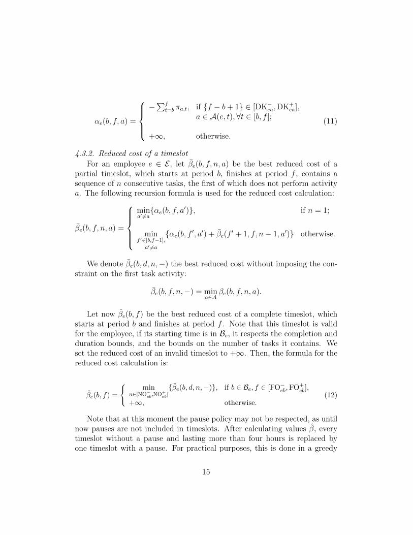
4.3.2. Reduced cost of a timeslot
For an employee e ∈ E , let βe(b, f, n, a) be the best reduced cost of apartial timeslot, which starts at period b, finishes at period f , contains asequence of n consecutive tasks, the first of which does not perform activitya. The following recursion formula is used for the reduced cost calculation:
βe(b, f, n, a) =
mina′ 6=aαe(b, f, a′), if n = 1;
minf ′∈[b,f−1],
a′ 6=a
αe(b, f ′, a′) + βe(f′ + 1, f, n− 1, a′) otherwise.
We denote βe(b, d, n,−) the best reduced cost without imposing the con-straint on the first task activity:
βe(b, f, n,−) = mina∈A
βe(b, f, n, a).
Let now βe(b, f) be the best reduced cost of a complete timeslot, whichstarts at period b and finishes at period f . Note that this timeslot is validfor the employee, if its starting time is in Be, it respects the completion andduration bounds, and the bounds on the number of tasks it contains. Weset the reduced cost of an invalid timeslot to +∞. Then, the formula for thereduced cost calculation is:
βe(b, f) =
min
n∈[NO−eb,NO+eb]βe(b, d, n,−), if b ∈ Be, f ∈ [FO−eb,FO+
eb],
+∞, otherwise.(12)
Note that at this moment the pause policy may not be respected, as untilnow pauses are not included in timeslots. After calculating values β, everytimeslot without a pause and lasting more than four hours is replaced byone timeslot with a pause. For practical purposes, this is done in a greedy
15

manner: we put the pause to a period in the second third of the timeslotsuch that its reduced cost is minimized. The pause replaces the correspondingwork period such that the duration of timeslot is not increased. Note that thisgreedy approach for inserting pauses makes the whole dynamic programmingprocedure heuristic (sub-optimal solutions may be generated).
If a pre-assigned pause is contained inside a timeslot, and it is not posi-tioned in the second third of it, such a timeslot is declared invalid, and itscost is set to +∞. The same happens if the employee cannot take any pause(P(e, t) is empty for all time moments in the second third of the timeslot).
Let βe(b, f) be the best reduced cost of a timeslot, which starts at periodb, finishes at period f , and respects the pause policy. Let `(b, f) be thistimeslot’s working time, which can be uniquely determined from its duration(f − d+ 1) according to the pause policy.
4.3.3. Reduced cost of a day-shift
For an employee e ∈ E , let δκe (d, b, f, `) be the best reduced cost of aday-shift of day d that starts at period b, completes at period f , containsκ timeslots and ` working periods. A valid day-shift should satisfy starting,completion, working time bounds and the daily pre-assignments. Let set Ωed
contain the set of valid triples (b, f, `):
Ωed =
(b, f, `) :
b ∈ [BD−ed,BD+ed], f ∈ [FD−ed,FD+
ed],` ∈ [LD−ed,LD+
ed], f − b+ 1 ≤ DD+ed
.
The formula for the day-shift containing one timeslot is:
δ1e(d, b, f, `) =
βe(b, f), if (b, f, `) ∈ Ωed, ` = `(b, f);
+∞, otherwise.(13)
The formula for the day-shift containing two timeslots separated by alunch break is:
δ2e(d, b, f, `) = min
f ′,b′
βe(b, f′) + βe(b
′, f), if (b, f, `) ∈ Ωed,` = `(b, f ′) + `(b′, f),b′ − f ′ − 1 ∈ [RD−ed,RD+
ed],`(b, f ′) ≥ TDed or`(b′, f) ≥ TDed;
+∞, otherwise.
(14)
16

The best reduced cost δe(d, b, f, `) of a day-shift with one or two timeslotscan now be computed :
δe(d, b, f, `) = minδ1e(d, b, f, `), δ
2e(d, b, f, `)
.
4.3.4. Reduced cost of an individual planning
In this step, we seek the best combination of day-shifts and days-off thatdesigns a valid individual planning for employee e given its total workingtime LEe and its number of day-shifts in [NE−e ,NE+
e ]. This is also called atour scheduling problem for a single employee.
For an employee e ∈ E , let η0e(d, n, `) be the best reduced cost of a par-
tial employee planning for the first d days, which contains n day-shifts and` working periods, and ends with a day-off. Let also η1
e(d, f, n, `) be thebest reduced cost of a partial employee planning for the first d days, whichcontains n day-shifts and ` working periods, and ends at period f with aday-shift. These reduced costs are calculated using the following recursions.We set η0
e(0, 0, 0) = 0, all other values η0e(0, f, `) are set to +∞. Also we set
η1e(d, f, n, `) = +∞ if d ≤ 0 or f 6∈ [FD−ed,FD+
ed].The formula for η0
e(d, n, `) is the following:
η0e(d, n, `) = min
η0e(d− 1, n, `),min
f
η1e(d− 1, f, n, `)
The formula for η1
e(d, f, n, `), f ∈ [FD−ed,FD+ed], is:
η1e(d, f, n, `) = min
η0e(d, f, n, `), min
f ′∈[FD−e,d−1,FD+e,d−1]
η1e(d, f
′, f, n, `)
, (15)
where η0e(d, f, n, `) is the best reduced cost with the condition that the em-
ployee had a day-off on day d−1, and η1e(d, f, f
′, n, `) is the best reduced costwith the condition that the employee had a day-shift of day d − 1 finishingat time f ′.
η0e and η1
e are computed as follows:
η0e(d, f, n, `) = min
b∈[BD−ed,BD+ed],
`′∈[LD−ed,LD+ed]
η0e(d− 1, n− 1, `− `′) + δe(d, b, f, `
′),
η1e(d, f ′, f, n, `) = minb∈[maxf ′+RE−e , BD−ed, BD+
ed
],
`′∈[LD−ed,LD+ed]
η1e(d− 1, f ′, n− 1, `− `′)+δe(d, b, f, `
′)
. (16)
17
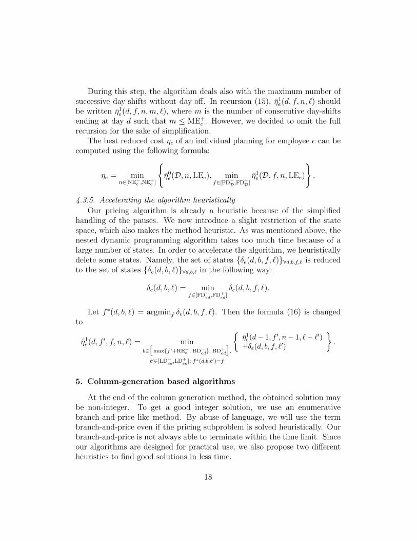
During this step, the algorithm deals also with the maximum number ofsuccessive day-shifts without day-off. In recursion (15), η1
e(d, f, n, `) shouldbe written η1
e(d, f, n,m, `), where m is the number of consecutive day-shiftsending at day d such that m ≤ ME+
e . However, we decided to omit the fullrecursion for the sake of simplification.
The best reduced cost ηe of an individual planning for employee e can becomputed using the following formula:
ηe = minn∈[NE−e ,NE+
e ]
η0e(D, n,LEe), min
f∈[FD−D,FD+D]η1e(D, f, n,LEe)
.
4.3.5. Accelerating the algorithm heuristically
Our pricing algorithm is already a heuristic because of the simplifiedhandling of the pauses. We now introduce a slight restriction of the statespace, which also makes the method heuristic. As was mentioned above, thenested dynamic programming algorithm takes too much time because of alarge number of states. In order to accelerate the algorithm, we heuristicallydelete some states. Namely, the set of states δe(d, b, f, `)∀d,b,f,` is reducedto the set of states δe(d, b, `)∀d,b,` in the following way:
δe(d, b, `) = minf∈[FD−ed,FD+
ed]δe(d, b, f, `).
Let f ∗(d, b, `) = argminf δe(d, b, f, `). Then the formula (16) is changedto
η1e(d, f
′, f, n, `) = minb∈[
maxf ′+RE−e , BD−ed, BD+ed
],
`′∈[LD−ed,LD+ed]: f∗(d,b,`′)=f
η1e(d− 1, f ′, n− 1, `− `′)
+δe(d, b, f, `′)
.
5. Column-generation based algorithms
At the end of the column generation method, the obtained solution maybe non-integer. To get a good integer solution, we use an enumerativebranch-and-price like method. By abuse of language, we will use the termbranch-and-price even if the pricing subproblem is solved heuristically. Ourbranch-and-price is not always able to terminate within the time limit. Sinceour algorithms are designed for practical use, we also propose two differentheuristics to find good solutions in less time.
18

5.1. Branch-and-price algorithm
Our branching scheme consists in fixing a variable xc,a,t for all candidatecolumns Xc related to a given employee e. In the formulation, this branchingis accomplished as follows:
• xc,a,t = 0 forbids employee e to be assigned to activity a at time periodt. We delete all columns Xc, c ∈ C(e), in which activity a is per-formed during period t. In the pricing subproblem for employee e, thecorresponding transition is forbidden.
• xc,a,t = 1 assigns employee e to production activity a at time period t.We delete all columns Xc, c ∈ C(e), in which activity a is not performedat period t. The subproblem for employee e is modified by assigning avery large negative cost to the corresponding transition.
When branching, we choose the triplet (employee e, production activ-ity a and time period t) which is the most fractional, i.e. for which |0.5 −∑
c∈C(e) xc,a,tqc| is minimum (where qc is determines whether individual plan-
ning Xc is chosen for employee e, as defined above). We use a depth-firststrategy to explore the search tree. We tried different strategies (sometimesmixed together): branching on the slack variables (under or over-coveragevariables), or branching on entities (forcing/forbidding an employee to workduring a given day or time-slot). However, we do not have convincing resultswhich show an advantage of these strategies over the scheme above.
The time allowed at each node of the branch-and-bound tree was limitedto one hour. In rare cases, this results in premature termination of columngeneration at some nodes. In that case, our heuristic branch-and-price con-tinues and carries out its branching strategy.
The heuristic dynamic programming algorithm for the subproblem makesour branch-and-price algorithm also heuristic. This means that theoreticallythere exist test instances for which the solution found is not optimal evenafter termination of the branch-and-price. However, for our test instancesthat are solved both by the branch-and-price and the MIP solver applied tothe compact formulation, the obtained solution values are equal.
5.2. Diving heuristic
The diving heuristic is an algorithm in which the branch-and-price tree issearched partially (see [26] for details). As usually done in diving heuristics,
19

we use a different branching strategy for the diving, as the goal here is notto have a balanced search tree, but a good feasible solution quickly. Assuggested in [26], at each node, after the termination of column generation,we select and fix a columnXc′ , i.e. we select a complete planning for employeee′ such that c′ ∈ C(e′). After that, all columns Xc, c ∈ C(e′), are excludedfrom the problem, demands DEa,t are updated according to the fixed partialsolution. Then, the subproblem for employee e′ is not called in descendantnodes.
As no backtracking occurs, the method stops after at most |E| nodes. Inour algorithm, we select the column related to the variable with the largestvalue in the solution of the master problem.
To obtain a fast heuristic, we introduce the time limit for column gener-ation at each node of the diving heuristic. When this time limit is reached,we use the current master solution values for fixing the next column, even ifthis solution is not optimal.
5.3. Greedy heuristic based on the nested dynamic program
When the time limit is set to a handful of seconds, the diving heuristicmay not be able to terminate. We propose a simple heuristic based on ourpricing subproblem to find good solutions in a small amount of time. Inthis heuristic, the employee plannings are still computed by our dynamicprogram, but the plannings are individually generated one by one and addediteratively to the solution. Here, the objective function of the subproblems isbased on the residual work demand REa,t, which corresponds to the remainingwork demand, taking into account the individual plannings already in thecurrent partial solution. Each time an individual planning is computed, theresidual work demand REa,t is updated, and the method is run again withthe remaining set of employees.
At initialization, REa,t have the same value as the work demand DEa,t
and they are updated each time a planning is added or deleted in the teamschedule. In the objective function of the subproblem for employee e, thecost πa,t of variable xa,t, which determines whether activity a is performedduring time period t, is calculated by the relation:
πa,t =
−REa,t/DEa,t − 1 if REa,t ≥ 0
−REa,t/DEa,t otherwise(17)
The greedy heuristic is presented formally in Algorithm 1. The first iter-ation is complete when the first complete solution is constructed. Then we
20

Algorithm 1:
1 Input: work demand DEa,t ;2 Best found solution is empty: Ωbest ← ∅;3 cost(Ωbest)← +∞;4 Partial solution is empty: Ω← ∅;5 E ′ ← Sort employees set E ;6 for i = 1, ..., nbIterations do7 foreach employee e ∈ E ′ do8 Delete current planning for employee e in partial schedule (if
exists): Ω← Ω \ Xc, c ∈ C(e) ;9 Compute the residual work demands ∀a, t:
REa,t ← DEa,t −∑
X∈Ω xa,t;10 Compute πa,t ∀a, t, according to (17);11 Solve subproblem with costs πa,t for employee e to obtain a
planning Xc, c ∈ C(e);12 Assign Xc to partial solution: Ω← Ω ∪ Xc;13 end14 if solution Ω is complete and cost(Ω) < cost(Ωbest) then15 Ωbest ← Ω;16 end
17 end18 return best found solution Ωbest ;
perform additional iterations in which, for each employee, the current individ-ual planning is deleted from the solution and another planning is computedbased on the updated residual work demand. Initial employees sorting, ob-jective function costs and the number of iterations are parameters of thealgorithm.
Despite our efforts, we did not find a particular sorting algorithm foremployees that gave better results than others on average. So we use Al-gorithm 1 several times with different random orders on the employees, andkeep the best result found. Empirical tests suggest that after three iterations,the solution is usually not improved anymore.
21

6. Computational experiments
Our four methods, solving MIP compact model by a commercial solver,the branch-and-price algorithm, the diving heuristic, and the greedy heuristichave been tested on both real data coming from a customer and randomlygenerated data. The MIP compact model is described in the electronic sup-plement.
6.1. Customer data
Data |E| |A| LBTriv greedy dive120 dive600 dive1800 B&P LBLagr compactA1-7 5 1 204 390 335 335 335 325 321,5 325A1-9 5 1 288 423 299 299 299 299 299 299A1-0 10 1 334 528 393 393 393 393 393 393A1-3 10 1 152 326 228 228 228 228 225,55 228A3-5 25 3 680 1077 832 834 832 824 T 819,7 890 TA3-9 25 3 866 1181 984 960 987 954 T 951 999 TA3-1 30 3 880 1285 970 962 954 954 T 935,4 1095 TA3-2 30 3 358 931 592 551 543 529 T 487,4 739 TA5-5 42 5 140 1111 918 909 852 852 T 804 3179A5-6 42 5 303 1254 1029 942 925 925 T 883,6 1298A5-0 45 5 404 1713 1522 1510 1504 1504 1504 -A5-1 45 5 412 1793 1529 1525 1533 1513 T 1507,7 -
Table 2: Customer data: solution values obtained by our methods. ”T”: branch-and-pricemethod and the MIP solver did not terminate within 24 hours of calculation. In this case,the solution value is the best one found ; ”-”: the MIP solver did not find any feasiblesolution within the time limit. The best found dive solution is used for initialisation ofthe B&P.
Our customer data comes from a company of mini-marts. All instancesare defined over one week divided into 15 minutes periods. In the customerdata, almost 10% of employees work only on Saturday, while the others maywork at most five days. Around 70% of the employees can only perform onetype of production activity. Most of the employees have a small flexibilityin their schedule: general beginning and finishing time of timeslots can beshifted by one hour (for instance, the first timeslot of a day-shift starts be-tween 8.00 AM and 9.00 AM for a given employee, but this range can bedifferent for another day).
22
Data |E| |A| greedy dive120 dive600 dive1800 B&P col. gen. compactA1-7 5 1 0,3 4,5 3,8 3,8 44,5 2,2 9,2A1-9 5 1 0,4 6,7 5,7 5,4 11,3 11,3 7,6A1-0 10 1 0,6 8,4 7,5 7,5 3,9 3,9 31135A1-3 10 1 0,5 13,6 12,8 12,5 2045 12,5 8962A3-5 25 3 1,6 118 482 833 T 105 TA3-9 25 3 2,0 118 574 1164 T 117 TA3-1 30 3 2,2 119 520 1163 T 546 TA3-2 30 3 2,2 127 617 1615 T 2642 TA5-5 42 5 2,8 131 592 1650 T 3663 TA5-6 42 5 2,7 135 592 1679 T 1244 TA5-0 45 5 2,3 123 527 1369 2166 2166 -A5-1 45 5 2,2 125 529 1102 T 177 -
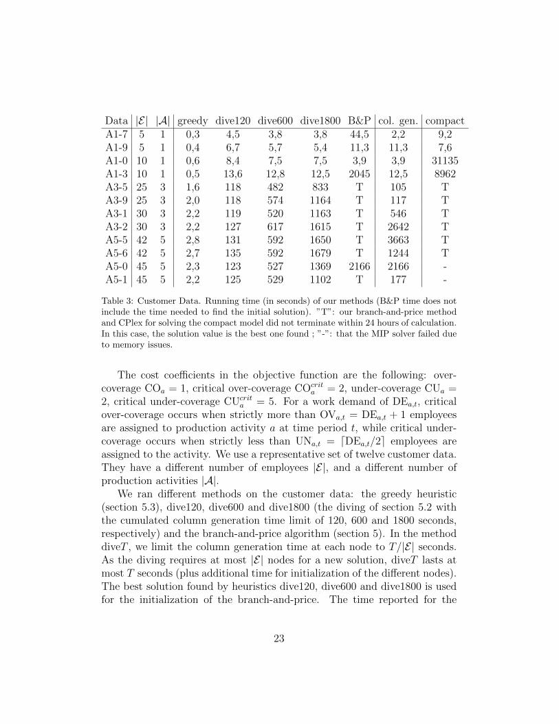
Table 3: Customer Data. Running time (in seconds) of our methods (B&P time does notinclude the time needed to find the initial solution). ”T”: our branch-and-price methodand CPlex for solving the compact model did not terminate within 24 hours of calculation.In this case, the solution value is the best one found ; ”-”: that the MIP solver failed dueto memory issues.
The cost coefficients in the objective function are the following: over-coverage COa = 1, critical over-coverage COcrit
a = 2, under-coverage CUa =2, critical under-coverage CUcrit
a = 5. For a work demand of DEa,t, criticalover-coverage occurs when strictly more than OVa,t = DEa,t + 1 employeesare assigned to production activity a at time period t, while critical under-coverage occurs when strictly less than UNa,t = dDEa,t/2e employees areassigned to the activity. We use a representative set of twelve customer data.They have a different number of employees |E|, and a different number ofproduction activities |A|.
We ran different methods on the customer data: the greedy heuristic(section 5.3), dive120, dive600 and dive1800 (the diving of section 5.2 withthe cumulated column generation time limit of 120, 600 and 1800 seconds,respectively) and the branch-and-price algorithm (section 5). In the methoddiveT , we limit the column generation time at each node to T/|E| seconds.As the diving requires at most |E| nodes for a new solution, diveT lasts atmost T seconds (plus additional time for initialization of the different nodes).The best solution found by heuristics dive120, dive600 and dive1800 is usedfor the initialization of the branch-and-price. The time reported for the
23
branch-and-price does not include the time spent by the heuristic. All testswere run using a standard PC of the experimental platform ”Plafrim” (seeAcknowledgement) with 4 GBits of memory over four cores (four subproblemsare solved in parallel). All methods were implemented in Java and IBM Cplex12.6 was used for solving the MIP and the linear master problems.
Tables 2 and 3 summarize the results obtained (respectively the objec-tive function value of the solution found, and the execution time) with ourcustomer data. In column ”LBLagr”, we report the Lagrangian lower bound(see subsection 3.3) computed at the root node of the B&P. Recall that |E| isthe number of employees, and |A| the number of production activities. Col-umn ”LBTriv” is a trivial lower bound computed in the following way. LetL be the cumulated working time of the team (measured in time periods):L =
∑e∈E LEe. Let also D be the cumulated demand (measured in time
periods): D =∑
t∈T∑
a∈ADEa,t. If D ≥ L then the solution value cannotbe less than LBTriv = mina∈ACUa × (D − L). If D < L then the solutionvalue cannot be less than LBTriv = mina∈ACOa × (L − D). The triviallower bound is quite far from the Lagrangian bound for the customer datainstances with 5 activities.
The running time of the greedy heuristic is very small, even for instanceswith 45 employees. The difference between the value of the greedy solutionand the optimal one can be large. However, recall that simple constructiveheuristics may fail to find feasible shifts, since assigning too much or toofew hours at the begining of the week may not allow to find a solution thatrespects all bound constraints. Moreover, the piecewise linear cost functionwill take a large value even if most of the working demand is fulfilled.
The diving heuristics are much more effective to find near optimal solu-tions for these instances. The relative gap of the dive120 heuristic with thebranch-and-price is greater than 10% only for two instances (A3 2 and A5 6).It may happen that the diving gives better results when a smaller comput-ing time is set (A3 5, A3 9 and A5 1). However, different experiments, notreported here, showed that giving more time to the diving heuristic at eachnode generally improves the result.
The branch-and-price method terminates for five instances out of twelvewithin 24 hours of computation time. For three instances the bounds aretight at the root node, for two instances the root ”lower bound” was improved(recall that the pricing is performed heuristically), for one instance the initialupper bound was improved, and for one instance both bounds were improvedby branch-and-price. For five instances out of the remaining six, branch-and-
24
price improves the upper bound before hitting the time limit. Note that whenthe MIP solver is able to find an optimal solution, its value is equal to thesolution value found by the heuristic branch-and-price.
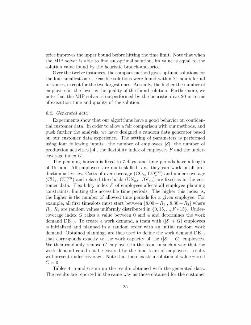
Over the twelve instances, the compact method gives optimal solutions forthe four smallest ones. Feasible solutions were found within 24 hours for allinstances, except for the two largest ones. Actually, the higher the number ofemployees is, the lower is the quality of the found solution. Furthermore, wenote that the MIP solver is outperformed by the heuristic dive120 in termsof execution time and quality of the solution.
6.2. Generated data
Experiments show that our algorithms have a good behavior on confiden-tial customer data. In order to allow a fair comparison with our methods, andpush further the analysis, we have designed a random data generator basedon our customer data experience. The setting of parameters is performedusing four following inputs: the number of employees |E|, the number ofproduction activities |A|, the flexibility index of employees F and the under-coverage index G.
The planning horizon is fixed to 7 days, and time periods have a lengthof 15 min. All employees are multi skilled, i.e. they can work in all pro-duction activities. Costs of over-coverage (COa, COcrit
a ) and under-coverage(CUa, CUcrit
a ) and related thresholds (UNa,t, OVa,t) are fixed as in the cus-tomer data. Flexibility index F of employees affects all employee planningconstraints, limiting the accessible time periods. The higher this index is,the higher is the number of allowed time periods for a given employee. Forexample, all first timeslots must start between J8.00−R1 , 8.30 +R2K whereR1, R2 are random values uniformly distributed in 0, 15, ..., F ∗ 15. Under-coverage index G takes a value between 0 and 4 and determines the workdemand DEa,t. To create a work demand, a team with (|E| + G) employeesis initialized and planned in a random order with an initial random workdemand. Obtained plannings are thus used to define the work demand DEa,t
that corresponds exactly to the work capacity of the (|E| + G) employees.We then randomly remove G employees in the team in such a way that thework demand could not be covered by the final team of employees: resultswill present under-coverage. Note that there exists a solution of value zero ifG = 0.
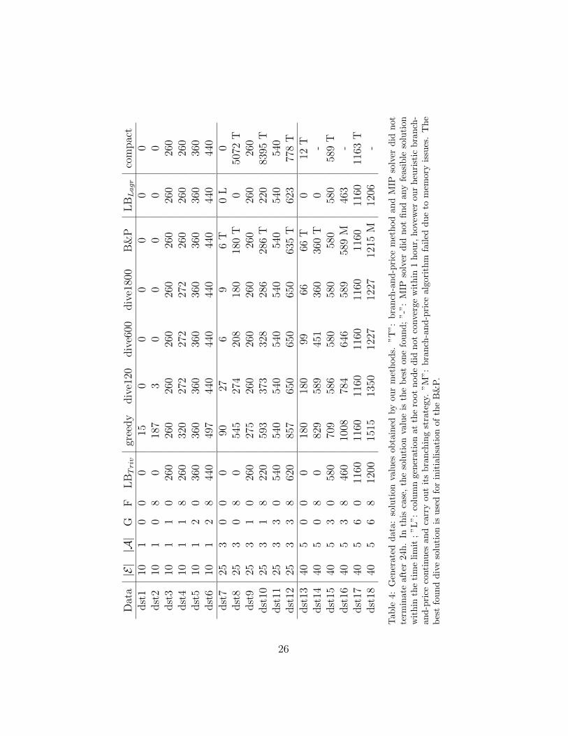
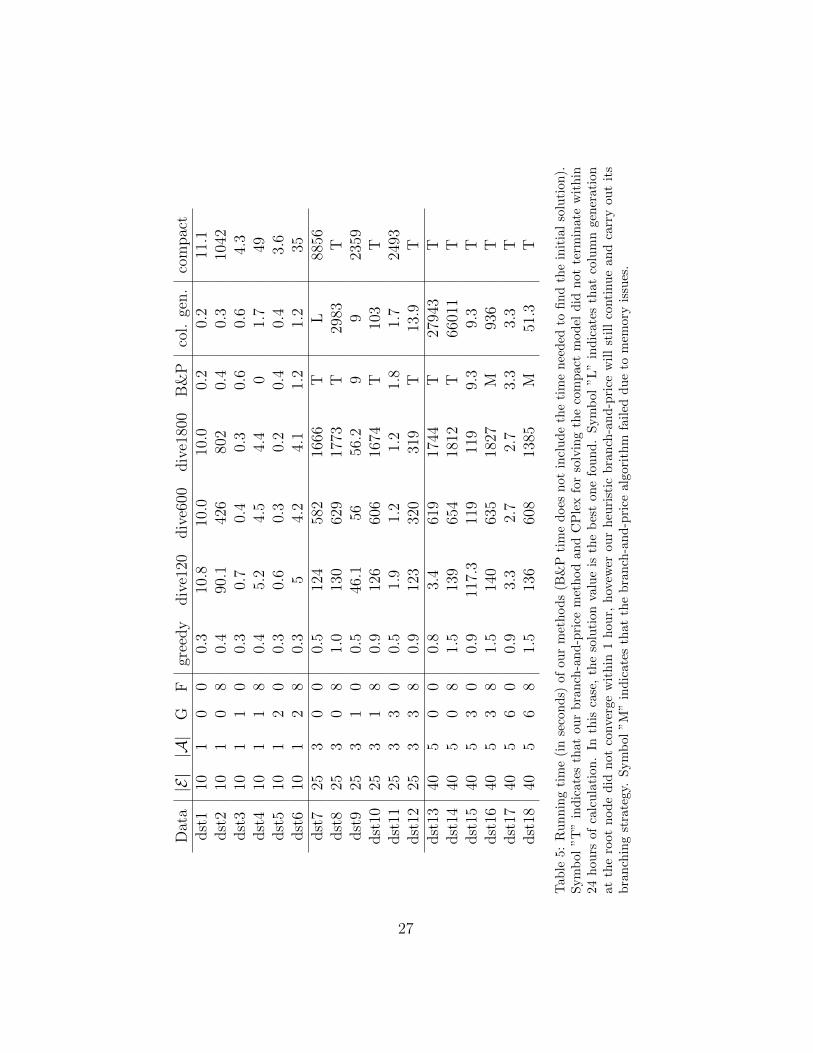
Tables 4, 5 and 6 sum up the results obtained with the generated data.The results are reported in the same way as those obtained for the customer
25
Dat
a|E||A|
GF
LBTriv
gree
dy
div
e120
div
e600
div
e180
0B
&P
LBLagr
com
pac
tdst
110
10
00
150
00
00
0dst
210
10
80
187
30
00
00
dst
310
11
026
026
026
026
026
026
026
026
0dst
410
11
826
032
027
227
227
226
026
026
0dst
510
12
036
036
036
036
036
036
036
036
0dst
610
12
844
049
744
044
044
044
044
044
0dst
725
30
00
9027
69
6T
0L
0dst
825
30
80
545
274
208
180
180
T0
5072
Tdst
925
31
026
027
526
026
026
026
026
026
0dst
1025
31
822
059
337
332
828
628
6T
220
8395
Tdst
1125
33
054
054
054
054
054
054
054
054
0dst
1225
33
862
085
765
065
065
063
5T
623
778
Tdst
1340
50
00
180
180
9966
66T
012
Tdst
1440
50
80
829
589
451
360
360
T0
-dst
1540
53
058
070
958
658
058
058
058
058
9T
dst
1640
53
846
010
0878
464
658
958
9M
463
-dst
1740
56
011
6011
6011
6011
6011
6011
6011
6011
63T
dst
1840
56
812
0015
1513
5012
2712
2712
15M
1206
-
Tab
le4:
Gen
erat
edd
ata:
solu
tion
valu
esob
tain
edby
ou
rm
eth
od
s.”T
”:
bra
nch
-an
d-p
rice
met
hod
an
dM
IPso
lver
did
not
term
inat
eaf
ter
24h.
Inth
isca
se,
the
solu
tion
valu
eis
the
bes
tone
fou
nd
;”-”
:M
IPso
lver
did
not
fin
dany
feasi
ble
solu
tion
wit
hin
the
tim
eli
mit
;”L
”:co
lum
nge
ner
atio
nat
the
root
nod
ed
idn
ot
conve
rge
wit
hin
1h
ou
r,h
ovew
erou
rh
euri
stic
bra
nch
-an
d-p
rice
conti
nu
esan
dca
rry
out
its
bra
nch
ing
stra
tegy.
”M
”:
bra
nch
-an
d-p
rice
alg
ori
thm
fail
edd
ue
tom
emory
issu
es.
Th
eb
est
fou
nd
div
eso
luti
onis
use
dfo
rin
itia
lisa
tion
of
the
B&
P.
26
Dat
a|E||A|
GF
gree
dy
div
e120
div
e600
div
e180
0B
&P
col.
gen.
com
pac
tdst
110
10
00.
310
.810
.010
.00.
20.
211
.1dst
210
10
80.
490
.142
680
20.
40.
310
42dst
310
11
00.
30.
70.
40.
30.
60.
64.
3dst
410
11
80.
45.
24.
54.
40
1.7
49dst
510
12
00.
30.
60.
30.
20.
40.
43.
6dst
610
12
80.
35
4.2
4.1
1.2
1.2
35dst
725
30
00.
512
458
216
66T
L88
56dst
825
30
81.
013
062
917
73T
2983
Tdst
925
31
00.
546
.156
56.2
99
2359
dst
1025
31
80.
912
660
616
74T
103
Tdst
1125
33
00.
51.
91.
21.
21.
81.
724
93dst
1225
33
80.
912
332
031
9T
13.9
Tdst
1340
50
00.
83.
461
917
44T
2794
3T
dst
1440
50
81.
513
965
418
12T
6601
1T
dst
1540
53
00.
911
7.3
119
119
9.3
9.3
Tdst
1640
53
81.
514
063
518
27M
936
Tdst
1740
56
00.
93.
32.
72.
73.
33.
3T
dst
1840
56
81.
513
660
813
85M
51.3
T
Tab
le5:
Ru
nn
ing
tim
e(i
nse
con
ds)
ofou
rm
eth
od
s(B
&P
tim
ed
oes
not
incl
ud
eth
eti
me
nee
ded
tofi
nd
the
init
ial
solu
tion
).S
ym
bol
”T”
ind
icat
esth
atou
rb
ran
ch-a
nd
-pri
cem
eth
od
an
dC
Ple
xfo
rso
lvin
gth
eco
mp
act
mod
eld
idn
ot
term
inate
wit
hin
24h
ours
ofca
lcu
lati
on.
Inth
isca
se,
the
solu
tion
valu
eis
the
bes
ton
efo
un
d.
Sym
bol
”L
”in
dic
ate
sth
at
colu
mn
gen
erati
on
atth
ero
otn
od
ed
idn
otco
nve
rge
wit
hin
1h
our,
hov
ewer
ou
rh
euri
stic
bra
nch
-an
d-p
rice
wil
lst
ill
conti
nu
ean
dca
rry
ou
tit
sb
ran
chin
gst
rate
gy.
Sym
bol
”M”
ind
icat
esth
atth
eb
ran
ch-a
nd
-pri
cealg
ori
thm
fail
edd
ue
tom
emory
issu
es.
27
cases. It transpires from our results that the structure of the data stronglyimpacts the algorithms behavior. As one would expect, the computing timedepends on the number of employees to schedule, and the number of produc-tion activities. Flexibility is also a difficulty factor: it increases the numberof possible shifts, and makes the dynamic program slower.
The tests on generated data confirm the conclusion drawn on the customerdata. We observe that the ”lower bound” obtained at the root node of theheuristic branch-and-price still has a very good value, i.e. it is often closeor equal to the optimal solution or the best solution found, and the finalabsolute gap is small, except for the instances with a large size, and a largeflexibility (dst8, dst10, and dst16).
The greedy heuristic is fast and the quality of the planning is good butrarely optimal. The diving heuristic gives results that are close to those of thebranch-and-price in most cases (the results are even optimal for small data).Similar to what happens with the customer instances, giving more time ateach node of the diving clearly improves the results on average, although itmay happen (dts7) that better results are obtained when less time is allowed.
A specificity of generated data instances is that the trivial lower boundis very close to the Lagrangian one and the optimal solution. Moreover, thebounds are equal for most of the instances. When this is the case, it is quiteeasy to find an optimal dual solution π (optimal Lagrangian multipliers)for the column generation algorithm. However, even when an optimal dualsolution is known, it takes a large number of iterations to find an optimalprimal solution of the linear relaxation of the master problem. This factexplains why known stabilization techniques such as dual smoothing do notimprove convergence of column generation. They are aimed at stabilizingaround the best dual solution. This does not help in our case as the optimaldual solution is already known.
7. Conclusion
In this paper, we describe efficient strategies for solving a real-life em-ployee scheduling problem that mixes days-off scheduling, shift scheduling,shift assignment, activity assignment, pause assignment and break assign-ment. Our approaches are based on the Dantzig-Wolfe decomposition, andwe have successfully implemented a heuristic branch-and-price algorithm,from which we derived a diving heuristic and a greedy algorithm. Thesemethods were tested on both customer and randomly generated data with
28
excellent results. The computational experiments show that the proposedapproaches yield optimal or near optimal solutions in many cases.
The behavior of our methods raises several questions. Since classicalstabilization strategies were not able to improve the convergence of the algo-rithm, we need a deeper analysis of the structure of the problem to come upwith new strategies dedicated to this kind of problems. As explained above,stabilization techniques acting in the dual space have a limited impact onthe convergence. Therefore, an effort should be done in developing primalstabilization strategies.
From a customer point of view, it would be interesting to consider the an-nualized workforce allocation problem, in which employees are scheduled overthe planning horizon of several weeks (up to a year). This problem includesconstraints linking successive weeks of work. Since solving this problem forone week is already challenging for state-of-the-art methodologies, we planto derive heuristics for these very large scale instances.
In this work, we consider independent employees, i.e. they perform ac-tivities independently of other employees. Another challenge would be toconsider activities or tasks that require simultaneous presence of several em-ployees with different skills.
Acknowledgment
The authors would like to thank the anonymous referees for their usefulcomments, which helped improving the presentation of the paper.
Experiments presented in this paper were carried out using the PLAFRIMexperimental testbed, being developed under the Inria PlaFRIM developmentaction with support from Laboratoire Bordelais de Recherche en Informa-tique and Institut de Mathematique de Bordeaux and other entities: ConseilRegional d’Aquitaine, FeDER, Universite de Bordeaux and CNRS(see https://plafrim.bordeaux.inria.fr/).
References
[1] O. Kabak, F. Ulengin, E. Aktas, S. Onsel, Y. Topcu, Efficient shiftscheduling in the retail sector through two-stage optimization, EuropeanJournal of Operational Research 184 (1) (2008) 76–90.
[2] G. Dantzig, A comment on Edie’s ”Traffic delays at toll booths”, Journalof the Operations Research Society of America 2 (3) (1954) 339–341.
29

[3] J. Van Den Bergh, J. Belien, P. De Bruecker, E. Demeulemeester,L. De Boeck, Personnel scheduling: A literature review, European Jour-nal of Operational Research 26 (3) (2012) 367–385.
[4] A. Ernst, H. Jiang, M. Krishnamoorthy, D. Sier, Staff scheduling androstering: A review of applications, methods and models, EuropeanJournal of Operational Research 153 (1) (2004) 3–27.
[5] M. I. Restrepo, B. Gendron, L.-M. Rousseau, Branch-and-price for per-sonalized multi-activity tour scheduling, Tech. rep., CIRRELT (2015).
[6] Q. Lequy, M. Bouchard, G. Desaulniers, F. Soumis, B. Tachefine, As-signing multiple activities to work shifts, Journal of Scheduling 15 (2)(2012) 239–251.
[7] C. Quimper, L. Rousseau, A large neighbourhood search approach tothe multi-activity shift scheduling problem, Journal of Heuristics 16 (3)(2010) 373–392.
[8] M. Restrepo, L. Lozano, A. Medaglia, Constrained network-based col-umn generation for the multi-activity shift scheduling problem, Interna-tional Journal of Production Economics 140 (1) (2012) 466–472.
[9] Q. Lequy, G. Desaulniers, M. Solomon, A two-stage heuristic for multi-activity and task assignment to work shifts, Computers and IndustrialEngineering 63 (4) (2012) 831–841.
[10] G. Thompson, M. Pullman, Scheduling workforce relief breaks in ad-vance versus in real-time, European Journal of Operational Research181 (1) (2007) 139–155.
[11] M. Widl, N. Musliu, The break scheduling problem: complexity resultsand practical algorithms, Memetic Computing 6 (2014) 97–112.
[12] M. Hojati, A. Patil, An integer linear programming-based heuristic forscheduling heterogeneous, part-time service employees, European Jour-nal of Operational Research 209 (1) (2011) 37–50.
[13] R. Stolletz, E. Zamorano, A rolling planning horizon heuristic forscheduling agents with different qualifications, Transportation ResearchPart E: Logistics and Transportation Review 68 (2014) 39–52.
30
[14] G. Eitzen, D. Panton, G. Mills, Multi-skilled workforce optimisation,Annals of Operations Research 127 (1-4) (2004) 359–372.
[15] M.-C. Cote, B. Gendron, L.-M. Rousseau, Grammar-based column gen-eration for personalized multi-activity shift scheduling, INFORMS Jour-nal on Computing 25 (3) (2013) 461–474.
[16] V. Boyer, B. Gendron, L. Rousseau, A branch-and-price algorithmfor the multi-activity multi-task shift scheduling problem, Journal ofScheduling 17 (2) (2014) 185–197.
[17] J. O. Brunner, R. Stolletz, Stabilized branch and price with dynamicparameter updating for discontinuous tour scheduling, Computers &Operations Research 44 (2014) 137 – 145.
[18] A. Dohn, A. Mason, Branch-and-price for staff rostering: An efficientimplementation using generic programming and nested column genera-tion, European Journal of Operational Research 230 (1) (2013) 157–169.
[19] G. Dantzig, P. Wolfe, Decomposition principle for linear programs, Op-erations research 8 (1) (1960) 101–111.
[20] R. Stolletz, Operational workforce planning for check-in counters at air-ports, Transportation Research Part E: Logistics and TransportationReview 46 (3) (2010) 414–425.
[21] J. Desrosiers, M. Lubbecke, A primer in column generation, in:G. Desaulniers, J. Desrosiers, M. Solomon (Eds.), Column Generation,Springer US, 2005, pp. 1–32.
[22] B. Maenhout, M. Vanhoucke, Branching strategies in a branch-and-priceapproach for a multiple objective nurse scheduling problem, Journal ofScheduling 13 (1) (2010) 77–93.
[23] P. Wentges, Weighted dantzig–wolfe decomposition for linear mixed-integer programming, International Transactions in Operational Re-search 4 (2) (1997) 151–162.
[24] F. G. Engineer, G. L. Nemhauser, M. W. Savelsbergh, Shortest pathbased column generation on large networks with many resource con-straints, Tech. rep., Georgia Tech, College of Engineering, School ofIndustrial and Systems Engineering (2008).
31

[25] L. Lozano, A. Medaglia, On an exact method for the constrained shortestpath problem, Computers & Operations Research 40 (2012) 378–384.
[26] C. Joncour, S. Michel, R. Sadykov, D. Sverdlov, F. Vanderbeck, Col-umn generation based primal heuristics, Electronic Notes in DiscreteMathematics 36 (2010) 695–702.
32

nbN
odes
nbM
PnbC
olum
ns
Dat
a|E|
div
e120
div
e600
div
e180
0B
&P
div
e120
div
e600
div
e180
0B
&P
div
e120
div
e600
div
e180
0B
&P
dst
110
1010
101
209
209
209
110
8910
8910
890
dst
210
1010
101
1116
2891
3234
158
9417
140
2288
50
dst
310
22
21
55
55
4040
4040
dst
410
1010
1048
9191
9117
629
329
329
312
80dst
510
22
21
33
33
2020
2020
dst
610
1010
101
9090
907
227
227
227
60dst
725
2525
251
T39
011
1924
3120
02T
3014
8068
1797
050
025
Tdst
825
2525
2513
2T
383
1388
2301
6870
T23
0167
9512
183
1684
50T
dst
925
2525
2580
226
830
522
933
4232
8033
3233
3244
8335
dst
1025
2525
2580
2T
339
1057
2076
2293
3T
2136
6380
1177
044
8335
Tdst
1125
22
21
88
88
175
175
175
175
dst
1225
2525
2592
0T
421
826
826
3191
2T
3002
4827
4827
6175
19T
dst
1340
140
4091
T9
701
1310
9758
T32
084
2616
423
3866
80T
dst
1440
4040
402
T24
069
412
2219
94T
1869
5522
1034
879
680
Tdst
1540
4040
401
313
261
256
2740
9535
7934
3429
0dst
1640
4040
4011
2927
971
813
5871
6721
3558
1711
470
2414
70dst
1740
22
21
1010
1010
354
354
354
580
dst
1840
4040
4011
5126
279
413
2113
007
2178
8339
1150
239
7319
Tab
le6:
Gen
erat
edD
ata:
Beh
avio
rin
dic
ator
of
the
met
hod
sacc
ord
ing
toth
ed
ata
set.
Sym
bol
”T
”in
dic
ate
sth
at
ou
rb
ran
ch-a
nd
-pri
cem
eth
od
did
not
term
inat
ew
ith
in24
hou
rsof
calc
ula
tion
.In
this
case
,th
eso
luti
on
valu
eis
the
bes
ton
efo
un
d.
33