College I and University Physics I - A Laboratory Manualbzeller/labmanual-p1-spring2016.pdf · College I and University Physics I - A Laboratory Manual Bruce W. Zellar Spring 2016

College I and University Physics I - A Laboratory

Manual

Bruce W. Zellar

Spring 2016 Addition

ii

c© Copyright, 2002, 2003, 2004, 2016 by the author, Bruce W. Zellar.Printed in the United States of America. All rights reserved. This book, orparts thereof, may not be reproduced in any form without written permissionof the author.

Contents

Preface xi

1 P1-1: Uncertainty in Measurements 1

1.1 Objectives . . . . . . . . . . . . . . . . . . . . . . . . . . . . 1

1.2 Significant Figures . . . . . . . . . . . . . . . . . . . . . . . . 1

1.2.1 Use of Significant Figures . . . . . . . . . . . . . . . . 2

1.2.2 Rules for Using Significant Figures in Calculations . . 2

1.3 Uncertainty or Error . . . . . . . . . . . . . . . . . . . . . . . 3

1.4 Precision and Accuracy . . . . . . . . . . . . . . . . . . . . . 4

1.5 Propagation of Error . . . . . . . . . . . . . . . . . . . . . . . 5

1.5.1 Absolute and Percent Error . . . . . . . . . . . . . . . 5

1.5.2 Rules Used To Calculate Uncertainty . . . . . . . . . . 5

1.5.3 Propagation of Error Examples . . . . . . . . . . . . . 6

1.6 Experimental Procedure . . . . . . . . . . . . . . . . . . . . . 8

1.6.1 Volume and Density of a Cylinder . . . . . . . . . . . 8

1.6.2 Equipment Usage . . . . . . . . . . . . . . . . . . . . . 8

1.6.3 Experimental Procedure . . . . . . . . . . . . . . . . . 10

1.6.4 Calculations . . . . . . . . . . . . . . . . . . . . . . . . 11

1.6.5 Questions . . . . . . . . . . . . . . . . . . . . . . . . . 11

1.6.6 P111/112 Data Sheet - Experiment 1: Error Analysis 13

2 P1-2:Statistical & Graphical Analysis 15

2.1 Objectives . . . . . . . . . . . . . . . . . . . . . . . . . . . . 15

2.2 Statistics . . . . . . . . . . . . . . . . . . . . . . . . . . . . . 15

2.2.1 Statistical Distributions . . . . . . . . . . . . . . . . . 16

2.2.2 An Example of Standard Deviation of the Mean . . . 18

2.3 Graphical Analysis . . . . . . . . . . . . . . . . . . . . . . . . 19

2.3.1 Regression Analysis . . . . . . . . . . . . . . . . . . . 20

iii

iv CONTENTS

2.3.2 How To Calculate a Least Squares Fit . . . . . . . . . 21

2.3.3 A Least Squares Fit Example . . . . . . . . . . . . . . 22


2.4.1 Part A: Statistical Determinations - Area of a Plate . 26

2.4.2 Part B: Regression Analysis - A Stone Thrown Vertically 28

2.5 Calculations . . . . . . . . . . . . . . . . . . . . . . . . . . . . 30

2.6 Questions . . . . . . . . . . . . . . . . . . . . . . . . . . . . . 30

2.7 Report Requirements . . . . . . . . . . . . . . . . . . . . . . . 30

2.7.1 P111/112 Results Summary Sheet - Experiment 2:Statistical and Graphical Analysis . . . . . . . . . . . 31

3 Uniform Acceleration 33

3.1 Objectives . . . . . . . . . . . . . . . . . . . . . . . . . . . . 33

3.2 Introduction . . . . . . . . . . . . . . . . . . . . . . . . . . 33

3.2.1 Uniform (Linear) Acceleration . . . . . . . . . . . . . 33

3.2.2 Experimental Concept . . . . . . . . . . . . . . . . . . 34


3.3.1 Materials . . . . . . . . . . . . . . . . . . . . . . . . . 35

3.3.2 Data Collection . . . . . . . . . . . . . . . . . . . . . . 35

3.4 Analysis . . . . . . . . . . . . . . . . . . . . . . . . . . . . . . 38

3.5 Questions . . . . . . . . . . . . . . . . . . . . . . . . . . . . . 39


4 Projectile Motion 41

4.1 Objectives . . . . . . . . . . . . . . . . . . . . . . . . . . . . 41

4.2 Introduction . . . . . . . . . . . . . . . . . . . . . . . . . . 41

4.2.1 The Range of the Projectile . . . . . . . . . . . . . . . 41

4.2.2 More on the Range . . . . . . . . . . . . . . . . . . . . 43

4.3 Experimental Concept . . . . . . . . . . . . . . . . . . . . . . 46


4.4.1 Materials . . . . . . . . . . . . . . . . . . . . . . . . . 46

4.4.2 Procedure (Determination of the range) . . . . . . . . 47

4.5 Calculations . . . . . . . . . . . . . . . . . . . . . . . . . . . . 48


5 Force & Static Equilibrium 53

5.1 Objectives . . . . . . . . . . . . . . . . . . . . . . . . . . . . 53

5.2 Introduction . . . . . . . . . . . . . . . . . . . . . . . . . . 53

5.2.1 Force . . . . . . . . . . . . . . . . . . . . . . . . . . . 53

5.2.2 Equilibrium . . . . . . . . . . . . . . . . . . . . . . . . 54

CONTENTS v



5.3.1 Materials . . . . . . . . . . . . . . . . . . . . . . . . . 55

5.3.2 Data Collection . . . . . . . . . . . . . . . . . . . . . . 56

5.4 Calculations . . . . . . . . . . . . . . . . . . . . . . . . . . . . 57

5.5 Questions . . . . . . . . . . . . . . . . . . . . . . . . . . . . . 57


6 Friction 61

6.1 Introduction . . . . . . . . . . . . . . . . . . . . . . . . . . . . 61

6.2 Theory . . . . . . . . . . . . . . . . . . . . . . . . . . . . . . . 61

6.2.1 Part A . . . . . . . . . . . . . . . . . . . . . . . . . . . 62

6.2.2 Part B . . . . . . . . . . . . . . . . . . . . . . . . . . . 63

6.2.3 Part C . . . . . . . . . . . . . . . . . . . . . . . . . . . 63

6.2.4 Optional Part D . . . . . . . . . . . . . . . . . . . . . 65

6.2.5 Optional Part E . . . . . . . . . . . . . . . . . . . . . 65


6.3.1 A - Static Friction. . . . . . . . . . . . . . . . . . . . . 65

6.3.2 Part B - Coefficient of kinetic friction using balancedforces. . . . . . . . . . . . . . . . . . . . . . . . . . . . 66

6.3.3 Part C - Coefficient of kinetic friction using unbal-anced forces. . . . . . . . . . . . . . . . . . . . . . . . 66

6.3.4 Part D Optional part Static Friction. . . . . . . . . . . 68

6.3.5 Part E Optional part Kinetic Friction. . . . . . . . . . 68

6.4 Calculations . . . . . . . . . . . . . . . . . . . . . . . . . . . . 69

6.5 Minimum Report Requirements . . . . . . . . . . . . . . . . . 69

7 Centripetal Force 71

7.1 Objectives . . . . . . . . . . . . . . . . . . . . . . . . . . . . 71

7.2 Introduction . . . . . . . . . . . . . . . . . . . . . . . . . . 71

7.2.1 Uniform Circular Motion and Centripetal Force . . . . 71



7.4 Calculations . . . . . . . . . . . . . . . . . . . . . . . . . . . . 77


8 Conservation of Energy 79

8.1 Objectives . . . . . . . . . . . . . . . . . . . . . . . . . . . . 79

8.2 Introduction . . . . . . . . . . . . . . . . . . . . . . . . . . 79

8.2.1 Work and Energy . . . . . . . . . . . . . . . . . . . . . 79

vi CONTENTS

8.2.2 Conservation of Mechanical Energy . . . . . . . . . . . 80



8.3.1 Materials . . . . . . . . . . . . . . . . . . . . . . . . . 81

8.3.2 Data Collection . . . . . . . . . . . . . . . . . . . . . . 82

8.4 Calculations . . . . . . . . . . . . . . . . . . . . . . . . . . . . 83

8.5 Questions . . . . . . . . . . . . . . . . . . . . . . . . . . . . . 84

9 Conservation of Linear Momentum 89

9.1 Objectives . . . . . . . . . . . . . . . . . . . . . . . . . . . . 89

9.2 Introduction . . . . . . . . . . . . . . . . . . . . . . . . . . 89

9.2.1 Momentum - Definition . . . . . . . . . . . . . . . . . 89

9.2.2 Types of Collisions . . . . . . . . . . . . . . . . . . . . 89

9.2.3 Conservation of Linear Momentum . . . . . . . . . . . 90



9.3.1 Materials . . . . . . . . . . . . . . . . . . . . . . . . . 93

9.3.2 Data Collection . . . . . . . . . . . . . . . . . . . . . . 93

9.4 Analysis & Calculations . . . . . . . . . . . . . . . . . . . . . 97

9.5 Questions . . . . . . . . . . . . . . . . . . . . . . . . . . . . . 97

10 Simple Harmonic Motion 101

10.1 Objective . . . . . . . . . . . . . . . . . . . . . . . . . . . . 101

10.2 Simple Harmonic Motion . . . . . . . . . . . . . . . . . . . . 101

10.2.1 The Static Displacement Of A Mass On A Spring . . . 101

10.2.2 The Oscillating Mass On A Spring . . . . . . . . . . . 102



10.3.1 Materials . . . . . . . . . . . . . . . . . . . . . . . . . 103

10.3.2 Part 1 - Static Displacement Case . . . . . . . . . . . 103

10.3.3 Part 2 - Oscillating Mass Case . . . . . . . . . . . . . 103

10.4 Analysis and Calculations . . . . . . . . . . . . . . . . . . . . 104

10.4.1 Static Case . . . . . . . . . . . . . . . . . . . . . . . . 104

10.4.2 Oscillating Case . . . . . . . . . . . . . . . . . . . . . 104

10.5 Questions . . . . . . . . . . . . . . . . . . . . . . . . . . . . . 104


11 Moment of Inertia 107

11.1 Objectives . . . . . . . . . . . . . . . . . . . . . . . . . . . . 107

11.2 Introduction . . . . . . . . . . . . . . . . . . . . . . . . . . 107

CONTENTS vii

11.2.1 Torque . . . . . . . . . . . . . . . . . . . . . . . . . . . 10711.2.2 Rotational Inertia (Moment of Inertia) . . . . . . . . . 10911.2.3 Relating Torque to Moment of Inertia . . . . . . . . . 10911.2.4 Moments of Inertia of Specific Objects. . . . . . . . . 11011.2.5 Experimental Concept . . . . . . . . . . . . . . . . . . 110

11.3 Experimental Procedure . . . . . . . . . . . . . . . . . . . . . 11211.3.1 Materials . . . . . . . . . . . . . . . . . . . . . . . . . 11211.3.2 Data Collection - Part A . . . . . . . . . . . . . . . . 11211.3.3 Data Collection - Part B . . . . . . . . . . . . . . . . . 112

11.4 Calculations . . . . . . . . . . . . . . . . . . . . . . . . . . . . 11311.5 Questions . . . . . . . . . . . . . . . . . . . . . . . . . . . . . 11411.6 Report Requirements . . . . . . . . . . . . . . . . . . . . . . . 114

12 Simple Pendulum 11712.1 Objective . . . . . . . . . . . . . . . . . . . . . . . . . . . . 11712.2 Period for the Small Angle Approximation . . . . . . . . . . . 11712.3 Experimental Procedure . . . . . . . . . . . . . . . . . . . . . 11912.4 Analysis and Calculations . . . . . . . . . . . . . . . . . . . . 12012.5 Report Requirements . . . . . . . . . . . . . . . . . . . . . . . 120

13 Vibrating String 12113.1 Objectives . . . . . . . . . . . . . . . . . . . . . . . . . . . . 12113.2 Introduction . . . . . . . . . . . . . . . . . . . . . . . . . . 121

13.2.1 A Pulse on a Rope . . . . . . . . . . . . . . . . . . . . 12113.2.2 Phase, Wavelength and the Fundamental Equation of

Wave Motion . . . . . . . . . . . . . . . . . . . . . . . 12213.2.3 Standing Waves . . . . . . . . . . . . . . . . . . . . . . 12313.2.4 Conditions for Standing Waves . . . . . . . . . . . . . 12413.2.5 Experimental Concept . . . . . . . . . . . . . . . . . . 124

13.3 Experimental Procedure . . . . . . . . . . . . . . . . . . . . . 12513.3.1 Materials . . . . . . . . . . . . . . . . . . . . . . . . . 12513.3.2 Data Collection . . . . . . . . . . . . . . . . . . . . . . 126

13.4 Calculations . . . . . . . . . . . . . . . . . . . . . . . . . . . . 12713.5 Questions . . . . . . . . . . . . . . . . . . . . . . . . . . . . . 12813.6 Report Requirements . . . . . . . . . . . . . . . . . . . . . . . 128

viii CONTENTS

List of Figures

1.1 Vernier Caliper . . . . . . . . . . . . . . . . . . . . . . . . . . 9

1.2 Micrometer Caliper . . . . . . . . . . . . . . . . . . . . . . . . 10

2.1 Gaussian Distribution (Bell Curve) . . . . . . . . . . . . . . . 16

2.2 Poisson Distribution . . . . . . . . . . . . . . . . . . . . . . . 17

2.3 Plot of 2x2 + 3 and 2[f(x)] + 3 with f(x) = x2 . . . . . . . . 21

2.4 Pressure as a function of Volume . . . . . . . . . . . . . . . . 23

2.5 Pressure as a function of Volume Squared . . . . . . . . . . . 24

2.6 Pressure as a function of Inverse Volume . . . . . . . . . . . . 25

3.1 Positions of a falling body. . . . . . . . . . . . . . . . . . . . . 34

3.2 Spacing of black bars on ”Picket Fence” ( c© 1991 PASCOScientific) . . . . . . . . . . . . . . . . . . . . . . . . . . . . . 35

3.3 Release position of ”Picket Fence” ( c© 1991 PASCO Scientific) 35

3.4 Photogate and ”Picket Fence” ( c© 1991 PASCO Scientific) . 36

4.1 Projectile Path . . . . . . . . . . . . . . . . . . . . . . . . . . 42

4.2 Pasco Projectile Launcher ( c© 1992 PASCO Scientific withmodifications.) . . . . . . . . . . . . . . . . . . . . . . . . . . 44

4.3 PASCO Short-Range Projectile Launcher. ( c© 1996-2012 PASCOScientific) . . . . . . . . . . . . . . . . . . . . . . . . . . . . . 45

5.1 Force Table Apparatus with three hanging masses. . . . . . . 55

5.2 Diagram of forces used in experiment. . . . . . . . . . . . . . 56

6.1 Experimental set-up. . . . . . . . . . . . . . . . . . . . . . . . 62

6.2 Free body diagram, static friction case. . . . . . . . . . . . . . 63

6.3 Free body diagram, kinetic friction case with acceleration. . . 64

6.4 Free body diagram, kinetic friction accelerating mass (M2). . 64

ix

x LIST OF FIGURES

7.1 Uniform circular motion. A particle travels around a circleat constant speed. . . . . . . . . . . . . . . . . . . . . . . . . 72

7.2 Centripetal force apparatus with clamp-on pulley and hang-ing mass. . . . . . . . . . . . . . . . . . . . . . . . . . . . . . 73

7.3 Centripetal force apparatus with clamp-on pulley and hang-ing mass. . . . . . . . . . . . . . . . . . . . . . . . . . . . . . 74

7.4 Close-up of spring, orange indicator and indicator bracket. . . 757.5 Close-up of side post assembly with object. . . . . . . . . . . 757.6 Close-up of rotating platform and bottom of side post assembly. 76

8.1 Diagram of experimental apparatus. ( c© May 1988 PASCOScientific with modifications.) . . . . . . . . . . . . . . . . . . 81

9.1 Two bodies both with non-zero initial velocities. . . . . . . . 909.2 Two bodies both with non-zero final velocities. . . . . . . . . 909.3 Two bodies collide and stick together. . . . . . . . . . . . . . 929.4 Apparatus with gliders and photogates. ( c© May 1988 PASCO

Scientific) . . . . . . . . . . . . . . . . . . . . . . . . . . . . . 92

10.1 Mass on a spring. . . . . . . . . . . . . . . . . . . . . . . . . . 102

11.1 Forces acting on a door - view from the top. . . . . . . . . . . 10811.2 Two forces acting on a body of arbitrary shape produce a

torque about point O. . . . . . . . . . . . . . . . . . . . . . . 10811.3 Moment of Inertia of an arbitrary body. . . . . . . . . . . . . 10911.4 Apparatus with rotating disk. . . . . . . . . . . . . . . . . . . 11111.5 Rotating disk with ring. . . . . . . . . . . . . . . . . . . . . . 111

12.1 Simple Pendulum. . . . . . . . . . . . . . . . . . . . . . . . . 118

13.1 A Pulse on a taut rope (left). Wave traveling along a rope(right). . . . . . . . . . . . . . . . . . . . . . . . . . . . . . . . 122

13.2 Transverse wave in a string. . . . . . . . . . . . . . . . . . . . 12313.3 Production of standing waves . . . . . . . . . . . . . . . . . . 12513.4 Vibrating String Apparatus. . . . . . . . . . . . . . . . . . . . 126

Preface

Ever since the beginning of the Twentieth Century, and perhaps even earlier,instruction in the Physics Laboratory has been designed to provide certainbenefits to the student. It is hoped that the student will learn skills that willhelp them develop discriminating powers of observation. The lab also putsthe student in personal contact with the general principles and phenomenadiscussed in both the textbooks and in the traditional lecture class.

Because of this, a strong emphasis has been put on determining the Erroror Uncertainty in measured and calculated quantities. It is equally impor-tant that the student learn to communicate the results of such an analysisand so, a report styled after a journal article is also stressed. Of course,the prose that each student generates in his or her reports will vary greatlyin sophistication from student to student, depending on the students back-ground and command of the English language, but as long as the studentdemonstrates the understanding of the matter at hand, this should not beheld against them. A sample report, tips on report writing and sampleuncertainty calculations can be found in the appendicies.

Many thanks to Dr. Ram Chaudhari (Professor Emeritus and of BlessedMemory) and Dr. Anne L. Caraley for their many helpful editorial com-ments.

xi

xii PREFACE

Experiment 1

P1-1: Uncertainty inMeasurements

1.1 Objectives

What are Significant Figures? What Rules Govern the Use of Significant

Figures? What is Uncertainty or Error? What is Absolute Uncertainty or

Absolute Error? What is Percent Uncertainty or Percent Error? What is

Propagation of Error and the Rules Governing It?? How is Uncertainty

calculated?

1.2 Significant Figures

The first step in the acquisition of experimental data is the direct observationof the relative position and motion of an object. Such an observation, ormeasurement, is possible only through the detection of sensations producedin the environment surrounding the object in question. The value of such anobservation depends on the accuracy of the measurement. The accuracy isalways limited by the refinement of the apparatus in use and the skill of theobserver. The accuracy can be improved with refinements in the measuringequipment and the observer’s skill in using it, but no matter how ’improved’the measurement is made, there is always a point when the observationbecomes uncertain. At this point, the measurement must be estimated.However, it gives information that is meaningful about the measurement in

1

2 EXPERIMENT 1. P1-1: UNCERTAINTY IN MEASUREMENTS

question and is therefore significant. We define a Significant Figure as onethat is know to be reasonably trustworthy.

1.2.1 Use of Significant Figures

This definition does not really seem very helpful, so here are a few rules thatwill clarify things.

The decimal place has nothing to do with the number of signifi-cant figures.

If a zero is used to merely indicate the location of the decimalplace, it is not significant.

If a zero is located between two figures that are significant, it isalways significant.

A zero located at the end of a number tends to be ambiguous.

Since the last digit in a measurement is uncertain and must beestimated, only one doubtful digit is kept and treated as signifi-cant.

For example, a certain length measurement is made using a meter-stickand is recorded as 7.36cm. The final digit, 6, is an estimate on the scale usingthe millimeter division. This reading has three significant figures. This samenumber can be written as 73.6mm and it also has three significant figures.Expressing this in meters gives 0.0736m or as 7.36 × 10−2m, once again,both expressions have three significant figures.

1.2.2 Rules for Using Significant Figures in Calculations

We now know how to specify the number of significant figures but we alsoneed to know how to use them in calculations. Numbers that do not repre-sent quantities that are measured have an unlimited number of significantfigures. For example, an inch is defined to be 2.54cm exactly. The 2.54 hasan unlimited number of significant figures. If it did not, then unit conver-sions would suffer unnecessary round-off and truncation errors. Likewise,pure numbers, such as Pi (π), also have unlimited significant figures.

When disregarding digits that are not significant, the digit to be retainedoften has to be rounded. For example, if a quantity is calculated to be 13.468

1.3. UNCERTAINTY OR ERROR 3

(which has 5 significant figures) and should only have 4 significant figures,then we round the 6 to a 7, so we would have 13.47, because we are droppingthe 8. If the 8 were instead a 2 (ie. 13.462), then we would round it to 13.46.When the digit to be dropped is 5, it is a bit more tricky. If the quantitywere 13.465, we would round it to 13.46. If it were 13.475, we would roundit to 13.48.

When adding or subtracting, it is convenient to arrange the numbersin columns to determine how many decimal places should be kept. Forexample,

Summarizing, we have five rules:

Any number that represents a numerical count in an exact defi-nition has an unlimited number of significant figures.

When a digit to be dropped is less than 5, the preceding digitis retained without change. When it is greater than 5, the lastdigit to be kept is rounded up by 1. When digit is exactly 5, thedigit to be kept is rounded so that the last digit kept is an evennumber.

When Adding or Subtracting numbers, arrange them in columnsand keep no column that is to the right of a column containinga doubtful figure.

When Multiplying or Dividing, the result should have no moresignificant figures than the factor having the least number ofsignificant figures.

The roots and powers of a number should have as many signifi-cant figures as the number itself.

1.3 Uncertainty or Error

In a physical experiment, one is faced with two types of determination ormeasurement; direct and indirect. A direct determination establishes a valuefor the quantity under consideration by the use of some kind of measuringdevice. An indirect determination involves one or more separate direct de-terminations which are used to find another physical quantity by means ofa functional relation (ie. a formula). The merit or reliability of such a de-termination is called the Uncertainty or Error. The word Error, doesnot mean mistake. A mistake can be corrected, but the Uncertainty can


never be eliminated, only reduced. The Uncertainty or Error is an inherent’fuzziness’ in the quantity. This fuzziness is random in nature.

At this point, it is convenient to discuss types of error, specifically thedifference between Systematic and Random Errors. When a given measure-ment is repeated several times, they generally do not agree exactly; this isthe result of a random error, which often comes about from a number offactors. Some of these are:

Errors of Judgment: Estimates of a fraction of the smallest di-vision of a a scale on an instrument may vary in a series ofmeasurements.

Fluctuation Conditions: Important factors in a given experimentsuch as temperature, pressure, or line voltage may fluctuate dur-ing the measurements, affecting the results.

Small Disturbances: Small mechanical vibrations, and the pickupof spurious electrical signals will contribute random errors tosome types measurement.

Lack of Definition in the Quantity Measured: For example, mea-surements with a micrometer of the thickness of a steel platehaving non-uniform surfaces will in general not be reproducible.

Randomness in the Quantity Measured: Repeated measurementsof the number of disintegrations per second in a radioactivesource will give different values because radioactive disintegra-tions occur randomly in time.

In contrast, Systematic Errors present in the measurement process will pro-duce a constant offset from the ’true’ value, in a series of repeated mea-surements. For example, a systematic error will be present if the measuringdevice is used improperly or if it is not calibrated correctly.

1.4 Precision and Accuracy

If the measured values cluster around a ’true’ value closely, the measurementis regarded as accurate. And, if an experiment has a small systematic errorit is regarded as having high accuracy. A precise measurement is one inwhich the spread of measured values is small, and, naturally, the sourceof the error is random. One should note that a measurement can be veryprecise but inaccurate if the systematic errors are large. One should keepthis in mind when one applies the following error analysis technique.

1.5. PROPAGATION OF ERROR 5

1.5 Propagation of Error

1.5.1 Absolute and Percent Error

The most natural way in which to judge the merit of an experimental valueis to compare it to an actual value, when it is know. One way to do this isto find the Percent Difference. The Percent Difference is defined as:

(accepted value−measured value)/(accepted value) ∗ 100% (1.1)

Close agreement would presume an ’accurate’ determination, but, in a ma-jority of cases, an actual value is not known. Furthermore, it is difficultto know when or if such a difference is significant. In that case, one canjudge the merit by examining the range of uncertainty of the determina-tion. This range in uncertainty is referred to as Absolute Uncertaintyor Absolute Error. For a direct measurement, the Absolute Uncertaintyor Absolute Error is an estimate (or educated guess). The observer assignsa value for the error based on a number of factors such as the fineness ofthe graduation of the measuring scale, the degree of estimation involvedin determining the final digit in the value, how the device is used to mea-sure, etc. A small absolute error indicates a precise determination. If themeasurement is repeated enough times, a statistical determination, such asthe standard deviation of the mean may be used instead of the estimation.This uncertainty can also be expressed as a percent. We define the PercentError as:

Percent Error = (Absolute Error)/(Quantity) ∗ 100% (1.2)

1.5.2 Rules Used To Calculate Uncertainty

For an indirect measurement, the determination is more complicated. Sincethis type of determination is not direct, it must be calculated. There aretwo rules by which this can be accomplished.

Rule I When two or more quantities are added and/or sub-tracted, the Absolute Error in the calculated quantity is foundby ADDING the Absolute Errors of the values used in thecalculation.

Rule II When two or more quantities are multiplied, dividedand/or raised to a power, the Percent Error in the calculatedquantity is found by ADDING the Percent Errors of the


values used in the calculation, and if a value is raised to a power,that particular value’s percent error is first multiplied by thatpower before the individual percent errors are added.

In calculations that involve combinations of addition, subtraction, multipli-cation, divison and raising to a power, the standard algebraic rules used toperform the calculation dictate when the above rules are applied.

1.5.3 Propagation of Error Examples

So, how do we use these rules? Let’s look at a simple case: a triangulartabletop. The tabletop is shaped as a right triangle with sides measuring3.0m ± 0.2m, 4.0m ± 0.2m and 5.0m ± 0.2m. What are the perimeter andarea of the tabletop with their respective uncertainties (ie. errors)?

Perimeter is defined as the addition of the lengths of the sides, so

P = a+ b+ c = 3.0m+ 4.0m+ 5.0m = 12.0m

The absolute error or absolute uncertainty for the perimeter is found byusing the rule for addition which is Rule I,

δP = δa+ δb+ δc = 0.2m+ 0.2m+ 0.2m = 0.6m

The percent error or percent uncertainty is,

(δP/P ) · 100% = (0.6m/12.0m) · 100% = 5.0%

The area is,

A = 1/2ab = (1/2)(3.0m)(4.0m) = 6.0m2

and the percent uncertainty for the area is given by Rule II,

(δA/A) · 100% = (0.2/3.0) · 100% + (0.2/4.0) · 100% = 11.6%

and the absolute uncertainty is,

(11.6%/100%) · 6.0m2 = 0.7m2

So, we would quote the values for the perimeter as,

12.0m± 0.6m or 12.0m± 5.0%

and for the area as,

1.5. PROPAGATION OF ERROR 7

6.0m2 ± 0.7m2 or 6.0m2 ± 11.6%

Notice, we have adjusted for the proper number of significant figures.Now, let us consider a more complicated situation. Suppose we want to

find the magnitude of a two dimensional vector given the vector’s x and ycomponents. The magnitude in the x direction is Fx = 5.0N ± 0.5N and inthe y direction Fy = 12.0N ± 0.5N . The magnitude of the two componentsis given by,

|F | =√F 2x + F 2

y =√

(5.0)2 + (12.0)2 = 13.0N

Now the uncertainty calculation is more complicated, because of theaddition of two squared quantities and then a square root. To apply bothRule I and Rule II, we follow the rules of algebra. Algebraic rules dictatethat each square be calculated first, then added, and finally the square rootis found. So the uncertainty is found as follows; percent error for Fx and Fy(using the definition of percent error),

(δFx/Fx) · 100% = (0.5N/5.0N) = 10.0%

(δFy/Fy) · 100% = (0.5N/12.0N) = 4.2%

The percent error in F 2x (using Rule II),

2 · 10% = 20%

The percent error in F 2y (using Rule II),

2 · 4.2% = 8.4%

The absolute error for F 2x and F 2

y (using the definition of percent errorbackwards),

(20.0%/100%) · (5.0N)2 = 5.0N2

(8.4%/100%) · (12.0N)2 = 12.0N2

The absolute error in the quantity, F 2x + F 2

y (using Rule I),

5.0N2 + 12.0N2 = 17.0N2

The percent error in the quantity, F 2x+F 2

y (using the definition of percenterror), (

17.0N2/169.0N2)· 100% = 10.0%


The percent error in the quantity,√F 2x + F 2

y (using Rule II)

1/2 · 10.0% = 5.0%

And, finally, the absolute error in |F | (using the definition of percenterror backwards),

(5.0%/100%) · 13.0N = 0.7N

1.6 Experimental Procedure

1.6.1 Volume and Density of a Cylinder

The volume of a uniform cylinder is given by

V = π(D2/4

)L (1.3)

where V is the volume, D is the diameter and L is the length. The densityis given by

ρ =m

V(1.4)

where ρ is the density and V is the volume. Measuring D, L and mdirectly, we will assign the uncertainty for each (see the above section ”Un-certainty or Error”). Then we can calculate V , ρ, δV and δρ; the latter twobeing indirect determinations.

1.6.2 Equipment Usage

Devices needed for measuring the lengths and diameters are: a ruler, avernier caliper and a micrometer caliper. For measuring the mass, a triplebeam balance will be used. Each of these instruments used to measurelength has a different degree of precision; the ruler having the least and themicrometer having the most.

Using a ruler is rather easy, line up one edge of the object in question witha tick mark on the ruler and then find the corresponding tick mark on theruler for the remaining edge. The difference between these two tick marksgives the length. Please note that this involves some degree of estimation andthis will help dictate the uncertainty assigned. The only other precautionone need take is to avoid using the edges of the ruler, since they may beworn down and hence introduce a systematic error in the measurement.

The vernier caliper and micrometer caliper are a bit more complicated.A vernier caliper is made up of a fixed jaw and a movable jaw (see figure

1.6. EXPERIMENTAL PROCEDURE 9

Figure 1.1: Vernier Caliper

1.1). The fixed jaw has a metric scale, called the main scale, which startsat 0mm and ends at 120mm. The movable jaw has a metric scale, calledthe vernier scale which starts at 0 and ends at 10. The leftmost mark onthe vernier scale has the value 0 (zero). When the jaws are closed, the zeromark (left most tick mark) on the vernier scale should line up with the zeromark on the main scale. If this is not the case, the vernier caliper is out ofcalibration. Do not use it and inform your instructor of this condition. Tomeasure the length of an object, open the jaws of the caliper wide enough forthe object to fit in between and then gently close the jaws so that fit snuglyagainst it. DO NOT TIGHTEN DOWN ON THE CALIPER!!! Itis not a ’C’ clamp! This will break it or put it out of calibration.

To determine the distance, as indicated by the spread of the jaws, lookfor the zero mark on the vernier scale. In the accompanying figure ( figure1.1) it lies between 13mm and 14mm. This means that the caliper readingis 13 plus ”something” mm. The ”something” part is found by finding thetick mark on the vernier scale that lines up with a tick mark on the mainscale. This will be unique for any given measurement. In the figure, the5 mark lines up the best with a mark on the main scale, hence the caliperreading is 13 + 0.5 = 13.5mm. Note that determining which mark on thevernier scale lines up best requires a degree of estimation and implies whatthe uncertainty might be.

The micrometer caliper also uses movable jaws and a vernier type scale.The movable part is called a thimble. The scale on the fixed jaw or main


Figure 1.2: Micrometer Caliper

scale has tick marks every 1mm above the horizontal line, and below theticks marks half way between. The thimble is graduated with 50 tick marks(on some types 100) and each rotation of the thimble moves it 0.5mm (or1.0mm), so each mark on the thimble is 0.5mm/50 = 0.01mm. To determinethe distance between the jaws, rotate the thimble until the jaws are spreadfar enough apart to allow the object to be inserted and then gently rotatethe thimble back until the jaws fit snugly against it. DO NOT TIGHTENDOWN ON THE CALIPER!!! It is not a ’C’ clamp! This willbreak it or put it out of calibration. To read the indicated value, locatethe edge of the thimble against the scale above the horizontal line on themain scale. In the accompanying figure (figure 1.2) the edge is between 3and 4, therefore the reading is 3 plus ”something” mm. Further, the edgeis also to the right of one of the tick marks below the horizontal line, soadd 0.5mm to the 3mm to obtain 3.5 plus ”something” mm. Lastly, thehorizontal line intersects the thimble at 37.5 (between thimble tick mark 37and 38), so the ”something” is 37.5 times 0.01mm = 0.375mm. This makesthe measurement 3.5 + 0.375 = 3.875mm. Note that the last digit is anestimate and gives a hint at the uncertainty.

1.6.3 Experimental Procedure

1. Record the alphanumeric identification stamped on your cylinder.

2. Using the following data sheet, measure and record the mass, diame-


ter and length of the cylinder using the ruler, vernier and micrometer. Also,record your estimates of the uncertainties (ie. absolute errors).

3. Make sure you record the measurements with the units common to theparticular device. Also, convert these to SI units and enter them on yourdata sheet.

1.6.4 Calculations

On a separate sheet of paper, calculate the Volume, V , the density δρ andthe absolute and percent errors for each. Present each calculation neatlyin three steps: write down the equation, then show how the values aresubstituted and then show the final numerical answer.

1.6.5 Questions

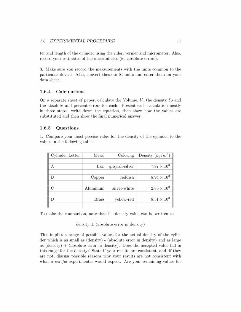
1. Compare your most precise value for the density of the cylinder to thevalues in the following table.

Cylinder Letter Metal Coloring Density (kg/m3)

A Iron grayish-silver 7.87× 103

B Copper reddish 8.94× 103

C Aluminum silver-white 2.85× 103

D Brass yellow-red 8.51× 103

To make the comparison, note that the density value can be written as

density ± (absolute error in density)

This implies a range of possible values for the actual density of the cylin-der which is as small as (density) - (absolute error in density) and as largeas (density) + (absolute error in density). Does the accepted value fall inthis range for the density? State if your results are consistent, and, if theyare not, discuss possible reasons why your results are not consistent withwhat a careful experimenter would expect. Are your remaining values for


the density consistent with the accepted value? Discuss along the same lines.

2. In the calculation section, you calculated the volume, V using

V = π(D2/4

)L (1.5)

An alternate formula that could have been used includes the radius, R,instead of the diameter:

V = π(R2)L (1.6)

If this had been used instead, would your uncertainties have been different?Why? (Show all work in support of your answer.)


1.6.6 P111/112 Data Sheet - Experiment 1: Error Analysis

Student’s Name:

Partner’s Name:

Lab Period: Date:

Instructor’s Signature or Initials:

Quantity Measuring Device Value Absolute Error

Mass Balance

g

kg

Length Ruler

cm

m

Vernier

cm

m

Micrometer

mm

m

Diameter Ruler

cm

m

Vernier

cm

m

Micrometer

mm

m

Cylinder Identification: Cylinder Metal:


Experiment 2

P1-2:Statistical & GraphicalAnalysis

2.1 Objectives

What is a Gaussian Distribution? What is the Standard Deviation? Whatis the Standard Deviation of the Mean? How is the Standard Deviationand Standard Deviation of the Mean use? What constitutes a good graph?What makes graphing important? What is a Linear Regression or RegressionAnalysis?

2.2 Statistics

As we have already see, every measurement we make has a certain uncer-tainty or error associated with it. Some of those errors are systematic, othersare random. A ruler used to measure the length of an object many times isan example of the latter. If we eliminate systematic errors, how much vari-ation can we expect in measuring a physical quantity once or many times?We could use the method illustrated in the previous experiment, but, thattends to overestimate the uncertainty and becomes impratical when largesets of data are involved. A better method is found in the mathematicalmethods of Statistics.

15

16 EXPERIMENT 2. P1-2: STATISTICAL & GRAPHICAL ANALYSIS

Figure 2.1: Gaussian Distribution (Bell Curve)

2.2.1 Statistical Distributions

If the error is truly random and the data are plotted on a Frequency Distri-bution Graph we get one of two distributions: Gaussian (a.k.a. Normal orBell Curve) or Poisson (see figures 2.1 and 2.2).

We note that the Gaussian Distribution is symmetrical and the that Pois-son Distribution is asymmetrical. The Poisson Distribution is asymmetricaldue to the mean of the distribution being bounded on one side.

Some important parameters of the Gaussian Distribution:1) Average or Mean

x =

N∑i=1

(x1 + x2 + x3 + ...+ xi)/N (2.1)

where N is the number of data points.

2.2. STATISTICS 17

Figure 2.2: Poisson Distribution


2) Deviation

Devi = (xi − x) (2.2)

3) Standard Deviation (SD)

SD =

√√√√ N∑i=1

(Devi)2/(N − 1) =

√√√√ N∑i=1

(xi − x)2/(N − 1) (2.3)

where N is the number of data points.

Physically, the standard deviation for a Gaussian Distribution means thefollowing: If one additional measurement of the quantity being measured istaken, the probability is 2/3 that the value of the measurement will lie inthe range: mean value ± one SD.

4) Standard Deviation of Mean

SDM = SD/√N (2.4)

Physically, the standard deviation of the mean for a Gaussian Distribu-tion means the following: If an additional set of measurements were taken,the probability is 2/3 that the mean value for this second set of measure-ments would lie in the range: previous mean ± one SDM .

2.2.2 An Example of Standard Deviation of the Mean

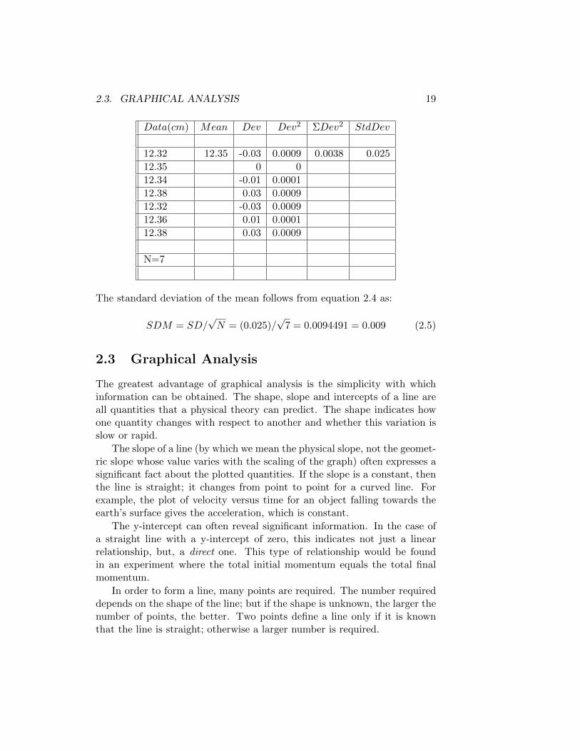
The accompanying table shows the results obtained when a student mea-sured the length of an object seven times. The student then used a spread-sheet and generated the standard deviation. Verify for yourself that themean, the deviations of each datum, the squares of each deviation, the sumof the squared deviations and the standard deviation are as shown.

2.3. GRAPHICAL ANALYSIS 19

Data(cm) Mean Dev Dev2 ΣDev2 StdDev

12.32 12.35 -0.03 0.0009 0.0038 0.025

12.35 0 0

12.34 -0.01 0.0001

12.38 0.03 0.0009

12.32 -0.03 0.0009

12.36 0.01 0.0001

12.38 0.03 0.0009

N=7

The standard deviation of the mean follows from equation 2.4 as:

SDM = SD/√N = (0.025)/

√7 = 0.0094491 = 0.009 (2.5)

2.3 Graphical Analysis

The greatest advantage of graphical analysis is the simplicity with whichinformation can be obtained. The shape, slope and intercepts of a line areall quantities that a physical theory can predict. The shape indicates howone quantity changes with respect to another and whether this variation isslow or rapid.

The slope of a line (by which we mean the physical slope, not the geomet-ric slope whose value varies with the scaling of the graph) often expresses asignificant fact about the plotted quantities. If the slope is a constant, thenthe line is straight; it changes from point to point for a curved line. Forexample, the plot of velocity versus time for an object falling towards theearth’s surface gives the acceleration, which is constant.

The y-intercept can often reveal significant information. In the case ofa straight line with a y-intercept of zero, this indicates not just a linearrelationship, but, a direct one. This type of relationship would be foundin an experiment where the total initial momentum equals the total finalmomentum.

In order to form a line, many points are required. The number requireddepends on the shape of the line; but if the shape is unknown, the larger thenumber of points, the better. Two points define a line only if it is knownthat the line is straight; otherwise a larger number is required.


2.3.1 Regression Analysis

The equation of a straight line is given by:

y = mx+ b (2.6)

where,

• x: is the independent variable, ie. abscissa (graph on horizontal axis)

• y: is the dependent variable, ie. ordinate (graph on vertical axis)

• m: is the slope of the line

• and b: is the y-intercept

Given a set of data which we suspect or believe fits a straight line (ie. islinear), we can use the method of Least Squares to obtain an equation thatrepresents the line defined by the data.

The basic principle of the Least Squares method is as follows:

The sum of the squares of the deviation of all points from thebest line (in accordance with this method) is the least it canbe. By the term deviation we mean the difference between they-value of the line and the y-value for the point (of the originaldata) for a particular value of x.

The application, by hand, of the Least Squares method is rather te-dious and leaves much room for mistakes in calculation; hence, we will usea computer spreadsheet and program it to do the tedious, mind-numbingcalculations.

Some important parameters generated by the Least Squares calculationare,

• X coefficient: (also known as slope of line)

• Std. Err. of Coef: (standard error of coefficient)

• R Squared: (measure of how good the data fit the equation. If RSquared = 1 implies a perfect fit.)

• y-intercept


Figure 2.3: Plot of 2x2 + 3 and 2[f(x)] + 3 with f(x) = x2

If the data points do not seem to fit a straight line, but we suspect theform of an equation that might, the Least Squares method can be extendedto this curve. In this case, the equation we fit is:

y = m[f(x)] + b (2.7)

so instead of plotting x on the horizontal axis, we plot f(x). For example,the following equation is not linear:

y = 2x2 + 3 (2.8)

As we can see (refer to figure 2.3), equation (2.8) is a parabola and (fromcalculus) its slope varies as 4x. But, if the values of x2 are plotted on thehorizontal axis and the values of y are plotted on the vertical axis, we get astraight line, for which the slope is 2 (a constant) and the y-intercept is 3,which follows from equation (2.7).

2.3.2 How To Calculate a Least Squares Fit

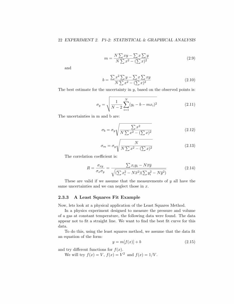
The best estimates for the slope and y-intercept are found from the following:


m =N∑xy −

∑x∑y

N∑x2 − (

∑x)2

(2.9)

and

b =

∑x2∑y −

∑x∑xy

N∑x2 − (

∑x)2

(2.10)

The best estimate for the uncertainty in y, based on the observed points is:

σy =

√√√√ 1

N − 2

N∑i=1

(yi − b−mxi)2 (2.11)

The uncertainties in m and b are:

σb = σy

√ ∑x2

N∑x2 − (

∑x)2

(2.12)

σm = σy

√N

N∑x2 − (

∑x)2

(2.13)

The correlation coefficient is:

R =σxyσxσy

=

∑xiyi −Nxy√

(∑x2i −Nx2)(

∑y2i −Ny2)

(2.14)

These are valid if we assume that the measurements of y all have thesame uncertainties and we can neglect those in x.

2.3.3 A Least Squares Fit Example

Now, lets look at a physical application of the Least Squares Method.In a physics experiment designed to measure the pressure and volume

of a gas at constant temperature, the following data were found. The dataappear not to fit a straight line. We want to find the best fit curve for thisdata.

To do this, using the least squares method, we assume that the data fitan equation of the form:

y = m[f(x)] + b (2.15)

and try different functions for f(x).We will try f(x) = V , f(x) = V 2 and f(x) = 1/V .


Figure 2.4: Pressure as a function of Volume

V olume(cm3) Pressure(kPa)

21 120

25 99.2

31.8 81.3

41.1 60.6

60.1 42.7

Slope (x-Coefficient) -1.869364912

Standard Error 0.344021941

y-intercept 147.6832639


R Squared 0.907768268


Figure 2.5: Pressure as a function of Volume Squared

V olume2(cm6) Pressure(kPa)

441 120

625 99.2

1011.24 81.3

1689.21 60.6

3612.01 42.7

Slope (x-Coefficient) -0.021474928




R Squared 0.817301612


Figure 2.6: Pressure as a function of Inverse Volume

1/V olume(cm−3) Pressure(kPa)

0.047619048 120

0.04 99.2

0.031446541 81.3

0.0243309 60.6

0.016638935 42.7

Slope (x-Coefficient) 2486.349853




R Squared 0.998085942

Looking at the regression output for f(x) = V , the R-Squared Coefficientis 0.9077, which might make one believe that this is the correct fit. In thecase where f(x) = V 2 the R-Squared Coefficient is smaller, 0.817. However,the last case, f(x) = 1/V has an R-Squared value of 0.998 making it thebest candidate so far, but, the R-Squared value is not the only criterionthat should be considered. Looking at the graph for f(x) = V , the plotshows a definite curvature, and not scatter about a best fit line. The plotof f(x) = 1/V shows a very straight line, and this is to be expected if theconditions of the experiment agree with PV = nRT , the ideal gas law.



2.4.1 Part A: Statistical Determinations - Area of a Plate

Imagine that a student has to measure very accurately the area of a rect-angular plate, whose dimensions are approximately 3.5 cm by 6.1 cm. Alogical choice of measuring device would be a vernier caliper. To accountfor irregularities in the sides the student makes measurements at several dif-ferent positions. The student also uses several different calipers to accountfor small biases in the measuring device. Use the following steps to findthe uncertainty in the area of the plate and to familiarize yourself with thecomputer spreadsheet, ”Excel”.

1. At your computer work station, open the folder labeled ”Physics Ap-plications”, which is located on the desktop of your computer screen.

2. Double click the icon for Microsoft Excel. (Star Office is available forthose who want it, but you are on your own.)

3. To enter something in a cell, first click it (if it is not already selected) andthen type in the desired contents, hitting the ”Enter” key when finished. Incell A1 type Width (cm) and in A13 Length (cm). To edit a cell, clickit and retype to correct or click on the edit line above the cell matrix andmove the cursor to the desired position and type or delete as necessary.

4. Enter the following data: in Cells A2 through A11, the Width; in CellsA14 through A23, the Length.


Width (cm) Length (cm)

3.435 6.036

3.436 6.035

3.433 6.041

3.438 6.037

3.434 6.036

3.435 6.032

3.433 6.039

3.436 6.038

3.433 6.036

3.434 6.038

5. Adjust the width of Column A so that the contents do not spill over ontoColumn B. This is done by positioning the cursor on the line separating thecolumn designators ”A” and ”B”, clicking and holding the left mouse buttonand dragging the line to the right. Make sure you do this each time a cellspills over onto another.

6. Add additional labels according to the following: Cell B1 Ave. Width;B13 Ave. Length; C1 Deviation; D1 Deviation Squared; E1 Sum ofSquared Deviations; F1 Standard Deviation

7. In Cell B2 type =AVERAGE(A2:A11) and in Cell B14 =AVER-AGE(A14:A23). Note, this gives the mean or average for the width andlength. The equal sign is necessary; it tells ”Excel” that you have entered aformula into a cell, not a label.

8. In Cell C2 type =A2-$B$2 and Cell C14 type =A14-$B$14. Thiswill give the deviation for the first data point for each dimension. Note thatthe ”$” before the column and row name makes this an absolute reference.This means no matter where the cell contents are copied, it will always ref-erence this exact cell.

9. To square the previous deviation type in Cell D2 =C2*C2 and in CellD14 =C14*C14

10. Use the ”Copy” and ”Paste” commands and copy the contents of CellC2 to Cells C3 through C11 inclusive. This will copy the formula for the


deviation and calculate the remaining deviations. To use the ”Copy” com-mand, select the desired cell (ie. Cell C2), click on the ”Edit” button abovethe cell matrix, click on ”Copy”. Now highlight the destination cells ( CellsC3 through C11) by clicking the left mouse button on the first cell of thedestination and hold it down and then drag until all of the desired cells areselected. Then, as before, click on ”Edit” and then click ”Paste”.

11. Now do the same for the squares of the deviations (ie Cell D2 etc.).Also, copy the labels in Cells C1 through F1 to Cells C13 through F13.

12. Complete the calculations for the deviations and squares of the de-viations for the lengths.

13. To sum the squares of the deviations, type in Cell E2 =SUM(D2:D11)and in Cell E14 =SUM(D14:D23).

14. To calculate the standard deviation, type in Cell F2 =SQRT(E2/(10-1)) and in Cell F14 =SQRT(E14/(10-1)). The 10 appears in the formulabecause there are 10 data points.

15. To print the graph, click ’File’ from the main window, then click ’PrintGraph’. On the pop-up window, click the check box next to ’Print Footer’and fill in the box with the names of the participants in this exercise. Inthe ’Comments’ box, put enough information to identify the trial that thisgraph represents and click ’OK’. The printer will be ’CutePDF Writer’. Thiswill allow you to print this to a file. The program will ask you to supply afilename and location to store it. For the filename, use something that willidentify the trial and use the ’Desktop’ for the location. You will have tosave this to a flashdrive or email it to your lab group as the computer willdelete it when you exit the current session.

2.4.2 Part B: Regression Analysis - A Stone Thrown Verti-cally

Imagine that a stone is thrown vertically upward with speed v. It shouldrise to a height h given by v2 = 2gh, where g is the local acceleration dueto gravity. This implies that a plot of v2 versus h will be a straight lineand its slope will be 2g. To test this, a student measures v2 and h for sevendiferent throws. Use the following steps to perform a linear regression and


graph the data.

17. Select a new sheet by clicking on the ”Sheet 2” Tab located at thebottom of the cell matrix. Enter a label in Cell A1 for the height, h, andvelocity squared, v2, in Cell B1. Enter the following data into the spread-sheet starting below the labels. Make sure you put the height and velocitysquared data in the correct columns.

h (m) v2 (m2/s2)

0.4 7

0.8 17

1.4 25

2.0 38

2.6 45

3.4 62

3.8 72

18. From the menu above the cell matrix, select ”Tools”, ”Data Analysis”,scroll down to find ”Regression” and select it. Then click the ”OK” but-ton. In the box marked ”Input Y Range” type =Sheet2!$B$2:$B$8 andin the box marked ”Input X Range” type =Sheet2!$A$2:$A$8. Underthe ”Output Options” click the circle button for ”Output Range” and type$A$10 in the box. Then click the ”OK” button.

19. Adjust the column widths for readability. Print out the spreadsheet.Sign and date it in the upper right hand corner.

20. To create a graph, click the ”Insert” button, located above the cellmatrix; click ”Chart”; choose ”XY(Scatter), then click the ”Next button.

21. To specify the X and Y series, click the ”Series” Tab and click the”Add” button. In the ”X Values” box type =Sheet2!$A$2:$A$8. Selectthe ”Y Values” box and type =Sheet2!$B$2:$B$8. In the ”Name” boxtype Stone. Then click ”Next”.

22. In the box for Chart Title type Velocity Squared vs. Height. TypeHeight (m) in the box labeled ”Value(X) axis:” and Velocity Squared(m2/s2) in the box for ”Value(Y) axis:”.


23. Set the vertical grid lines by clicking the ”Gridlines” Tab, then click thecheck box for ”Minor gridlines” under ”Value(X) axis” . Leave the checkbox for ”Major gridlines” under ”Value(Y) axis” selected. Click ”Next”.

24. To finish the graph, position the cursor over one of the data pointson the graph and click the right button of the mouse to get the pop-upmenu. Select ”Add Trendline...”. Select ”Linear” and then click ”OK”.

25. Make sure your lab partners have received a working copy of yourspreadsheet.

2.5 Calculations

1. Using the results of Procedure Part A, calculate the average area of theplate [A = l × w] and the Standard Deviation of the Mean for the averagelength and average width. Treat these as the Absolute Uncertainties andcalculate the Absolute and Percent Uncertainties in the area. Quote theresult to the proper number of significant figures.

2. From the slope of the line in Procedure Part B, determine the valueof g and its Absolute and Percent Uncertainty. The slope of the line is givenin the regression output in the row marked ”X Variable 1” and under thecolumn marked ”Coefficients”. The corresponding Standard Deviation isunder ”Standard Error”, in the same row. Quote g to the proper numbersignificant figures.

2.6 Questions

1. Assuming the local value of g is 9.81 m/s2, compare this value to theresult you got in Calculation step 2. Would you consider these two valuesto be the same? Why?

2.7 Report Requirements

1. Submit a working copy of your spreadsheet via email.2. Submit your sample calculations in a pdf via email if you have not alreadyincluded them in your spreadsheet.3. Submit your answer to Question 1 from above.

2.7. REPORT REQUIREMENTS 31

2.7.1 P111/112 Results Summary Sheet - Experiment 2: Sta-tistical and Graphical Analysis

Student’s Name:

Partner’s Name:

Lab Period: Date:

Instructor’s Signature or Initials:

Quantity Value Absolute Error Percent Error

Part A

length (cm)

width (cm)

area (cm2)

Part B

slope (m/s2)

g (m/s2)


Experiment 3

Uniform Acceleration

3.1 Objectives

To study the motion of a body falling freely in the near earth gravitationalfield.

3.2 Introduction

3.2.1 Uniform (Linear) Acceleration

According to Newton’s Law of Gravitation, a body falling near the surfaceof the Earth1 should appear to fall at a constant rate. In order to determinethe type of motion that this falling body undergoes, it is important to use amethod that is independent of any assumptions about that type of motion.The equations of uniform motion do not fulfill this requirement in this caseand so may not be used. Instead, the position of the falling body withrespect to time and the definitions of average velocity and acceleration willbe used. Consider three consecutive positions of the falling body; positionsa, b and c (see Figure 3.1). The average velocity of the body at position bis given by:

vb = (sc − sa)/(tc − ta) (3.1)

where, sc − sa is the displacement between points c and a and tc − ta is thetime it takes to go from a to c. It is important to note the t represents clocktime, not time interval. Whereas, tc − ta is a time interval.

If we determine the average velocity for each position and plot it againstthe time, the slope of the resulting curve will give the average acceleration

1Or any other planet or moon

33

34 EXPERIMENT 3. UNIFORM ACCELERATION

Figure 3.1: Positions of a falling body.

experienced by the body. Further, if the acceleration is constant, then theline will be straight and the motion observed will be uniform. Since theacceleration is by definition the change in velocity versus the change in time,the slope of such a line will give the average acceleration. In this particularcase, this acceleration corresponds to the local acceleration due to gravitydenoted by g.

3.2.2 Experimental Concept

The apparatus consists of a photogate and a ”Picket Fence”. The PicketFence is a rectangular piece of plastic that has evenly spaced opaque blackbars and when dropped through the photogate the black bars interrupt thelight beam. (See Figure 3.2)

If the distance between the black bars is known then the timing mea-surements from the photogate can be used to calculate the average velocity2

and a graph of velocity versus time will give a straight line whose slope isthe average acceleration.

2For the method used to calculate the velocity see - William J. Leonard, ”Dangers ofAutomated Data Analysis”, The Physics Teacher 35(4), 220-222 (Apr. 1997).


Figure 3.2: Spacing of black bars on ”Picket Fence” ( c© 1991 PASCO Sci-entific)

Figure 3.3: Release position of ”Picket Fence” ( c© 1991 PASCO Scientific)


3.3.1 Materials

1 - Picket Fence, 1 - photogate, 1 - LabPro interface, 1 - bench clamp, 1 -half-inch diameter rod, 1 - right angle clamp, 1 - thick foam pad or othersuitable padding (used to cushion the impact of the Picket Fence with thefloor).

3.3.2 Data Collection

Precautionary Notes

1) Make sure to place soft padding below the photogate to cushion the fallof the Picket Fence.

2) For an accurate result position and hold the Picket Fence according to


Figure 3.4: Photogate and ”Picket Fence” ( c© 1991 PASCO Scientific)

Figure 3.3. Pinch the end of the Picket Fence with your thumb and forefin-ger, centered at the top before releasing.

Procedure

1) Open the Logger Pro 3.3 software (located in the Desktop window). ClickFile, Open and the folder called Physics with Vernier. Scroll throughthe listings and select the file called ’05 Picket Fence Free Fall’. This willbe near the beginning of the listing. Two graphs should now be displayed;one labeled with Distance and Time and the other with Velocity and Time.

2) Position the Picket Fence just above the photogate so that it passesthrough as is illustrated in Figure 3.4.

3) Click the green ’Collect’ icon. The timer will start timing when thePicket Fence blocks the photodiode. The timing should stop by itself aftera pre-set interval. If it does not, stop the timing by clicking the red ’Stop’icon after the Picket Fence clears the photogate. The software is alreadyprogrammed with the black bar spacing of 5.00 cm.

4) You should now see the data plotted on both graphs. The data werecalculated by the software in accordance with equation 3.13. The velocitygraph should be a straight line and there should be more than three datapoints. If not, start this trial again. If you have trouble, please alert yourinstructor or the laboratory manager.

5) To select the data you wish to fit, click the left mouse button on the

3with some modifications


left most data point, hold it and drag across to the last datum. Your datashould now be highlighted. If you are having trouble, call for help.

6a) Click the Distances vs. Time graph. Click Analyze and LinearFit. A best fit line will be drawn thorough your data and a box with thebest fit information will appear. Then right click the dialog box that con-tains the linear fit information and choose Linear Fit Options. UnderStandard Deviations click the Slope box then OK. The standard devi-ation of the slope should now be displayed. Record the m(Slope), Std.Dev. of Slope and Correlation values. The former is the slope of the lineand the latter is the goodness of fit or R-Squared value. The R-Squaredshould always be 1 or very very close to that value. The middle value givesa statistical uncertainty in the value of the slope. Record all of the valuesfor this fit.

6b) For the same graph, repeat best line fitting steps only this time chooseCurve Fit instead of Linear Fit, then choose the Quadratic and thenOK. The software will most likely place the dialog boxes at inconvenientplaces on the graph. To remedy this, use the ’Click, Hold and Drag’ methodand move the boxes to spots that do not obscure the data and lines. Record’a’, ’b’ and ’c’ with their given statistical uncertainties and the ’RMSE’value. The ’RMSE’ is related to the quality of fit for this curve4.

6c) Click on the Velocity vs. Time graph and perform a linear fit us-ing your newfound skills and record all the relevant information. The slopeof this line is the average acceleration of the picket fence.

7) Repeat step 2) through 6) for a minimum of 8 to 10 trials or more ifwarranted.

8) To print the graph, click File from the main window, then click PrintGraph. On the pop-up window, click the check box next to Print Footerand fill in the box with the names of the participants in this exercise. Inthe Comments box, put enough information to identify the trial that thisgraph represents and click OK. The printer will be ’CutePDF Writer’. Thiswill allow you to print this to a file. The program will ask you to supply afilename and location to store it. For the filename, use something that will

4You may note that the quadratic is a better fit than the linear one by visual inspectionof the two fitted lines.


identify the trial and use the ’Desktop’ for the location. You will have tosave this to a flashdrive or email it to your lab group as the computer willdelete it when you exit the current session.

3.4 Analysis

In the table titled ’Sample Results’ you will find the results of this experi-ment conducted by another person and for the purposes of discussion let uscall that person Ima Yutz. Since each trial has its own variation (i.e. is madeup of a set of values for the acceleration), one cannot simple average themtogether and call that value the average of the acceleration. The variationof each trial must be taken into account. The solution to this problem is aquantity called the weighted average. The formal definition of the weightedaverage is: If x1, x2, ..., xN are measurements of a single quantity called xwhich have known uncertainties σ1, σ2, ..., σN , then the best estimate for xis calculate using

xwav =

∑wixi∑wi

(3.2)

where the sums are over all N measurements, i = 1, 2, ..., N , and the weightswi are the reciprocal squares of the corresponding uncertainties,

wi =1

σ2i

. (3.3)

The uncertainty in xwav is

σwav =1√∑wi, (3.4)

where the sums are over all of the measurements i = 1, 2, ..., N .For practice, see if you can duplicate Yutz’s final result before you do

you own calculation or pester your instructor for help.

3.5. QUESTIONS 39

Sample Results - by Ima Yutz

Acceleration (m/s/s) Standard Deviation (m/s/s) wi (wi)(ai)

9.761 0.0695 207.0286217 2020.806376

9.812 0.0917 119.051552 1168.133828

9.770 0.0572 305.531579 2985.043526

9.748 0.0488 419.9140016 4093.321688

9.924 0.0644 241.2670729 2394.334431

9.761 0.0690 210.1617228 2051.388576

9.851 0.0352 806.6180755 7945.994661

9.760 0.0241 1718.879346 16776.26241

9.723 0.0521 368.6871905 3584.745553

9.767 0.0588 289.1329859 2823.961873

9.715 0.0469 455.5969516 4426.124385

SUM = 5141.869099 50270.11731

awav = 9.777

swav = 0.014

1) Find the weighted average and the associated uncertainty for youracceleration. Call the average value gwav. Use Excel or your favorite spread-sheet software to make the tedious calculations less boring.

2) Compare gwav ± swav to both 9.805 m/s2 and the sample calculation.

3.5 Questions

1) Comment on the comparison from calculation step 2.

2) Do your results support the hypothesis that a body falling near the surfaceof the Earth undergoes uniform acceleration? Why?


1. Submit your completed Data/Calculations Sheet.

2. Submit your printed trial from Logger Pro and your Excel Spreadsheet


Sheet.

3. Answer the question(s) if assigned by your instructor.

4. Make sure you have your name and your lab partners names writtenon the top right hand side of EACH sheet of paper submitted. This is toensure that your work does not get lost should any of the pages get sepa-rated.

Experiment 4

Projectile Motion

4.1 Objectives

4.2 Introduction

The motion of a projectile is a special case of a freely falling body in whichthe initial velocity may be in any direction with respect to the vertical. Thepath of the projectile is a parabolic path produced by a combination of theuniform horizontal velocity of projection and the changing vertical velocitycaused by the acceleration of gravity. We can study this type of motionvery effectively by considering it as made up of two independent motions,one of constant velocity in the horizontal direction, and the other of constantacceleration in the vertical direction. In the detailed analysis of projectilemotion which follows we neglect air resistance, because its effects are smallin this experiment.

4.2.1 The Range of the Projectile

If we put the origin of the coordinate system used to describe the motionat the place of projection (making x0 and y0 = 0), then the two equationswhich describe the motion are

x = v0xt (4.1)

y = v0y +1

2gt2 (4.2)

where x and y are the horizontal and vertical positions of the object at thetime t, v0x is the initial velocity of the object in the x-direction, v0y the

41

42 EXPERIMENT 4. PROJECTILE MOTION

Figure 4.1: Projectile Path

initial velocity in the y-direction, and g the acceleration in the y-direction.For the object projected in Figure 4.1, these equations reduce to:

x = v0(cosθ)t (4.3)

y = v0(sinθ)t− 1

2gt2 (4.4)

Note that g is negative because it is in the negative direction as we havedefined it here. When the projectile hits the floor we know that x = R andy = −H. The value of y is negative because the floor is below the origin ofour coordinate system. With these substitutions, the equations become

R = v0(cosθ)t (4.5)

−H = v0(sinθ)t− 1

2gt2 (4.6)

In these equations the range R is the dependent parameter and v, H andθ are the independent parameters. In order to compare the theoretical rangewith the experimental range, we must measure the independent parametersand use these last two equations to calculate the range.

4.3. EXPERIMENTAL CONCEPT 43

4.2.2 More on the Range

Notice that in the above we did not say anything about measuring time.Recall that θ, v and H are the indedendent variables and that

R = v0(cosθ)t (4.7)

which implies

t =R

v0cosθ(4.8)

Substitute for t in

−H = v0(sinθ)t− 1

2gt2 (4.9)

gives

0 = H +R(tanθ)− g

2v20cos

2θR2 (4.10)

Now to complete this we need the quadratic formula. Putting the previousequation into standard form

− g

2v20cos

2θR2 + (tanθ)R+H = 0 (4.11)

and comparing to

Ax2 +Bx+ C = 0 (4.12)

and if we also let x = R then

A =−g

2v20cos

2θ(4.13)

B = tanθ (4.14)

and

C = H (4.15)

Now we can calculate numerical values for A, B and C and then substitutethe resultant numerical values into

R =−B ±

√B2 − 4AC

2A(the quadratic formula) (4.16)

to find the theoretical range. Note, you will get two values for the range,only one will make physical sense and it will be obvious to you which valueit is.


Figure 4.2: Pasco Projectile Launcher ( c© 1992 PASCO Scientific with mod-ifications.)

4.3. EXPERIMENTAL CONCEPT 45

Figure 4.3: PASCO Short-Range Projectile Launcher. ( c© 1996-2012PASCO Scientific)


4.3 Experimental Concept

The projectile launcher apparatus is depicted in Figures 4.2 and 4.3. Itconsists of a base that supports the launcher above a mounting surface suchas a bench or table. The base is secured to the mounting surface with twobench clamps. The launcher is attached to the base by two thumb screwsthat allow the launcher to be aimed at any angle from zero to ninety de-grees with respect to the mounting surface. The angle is determined usinga protractor with a small plumb bob and is located at the back end of thelauncher for easy access and can be determined to within one-half of a degree.

Loading and arming the launcher is accomplished by insertion of the pro-jectile through the front end into a cradle attached to a piston which is thenpushed into one of three locked positions with a ramrod. Once armed, theramrod is removed. If desired, the launcher may sighted at a target usingthe bore-sight located at the back end of the launcher prior to loading. Thepiston is connected to a spring that propels the cradle with the projectileup the barrel.

Pulling the trigger releases the cradle from the locked position. There isno spin imparted to the projectile since the cradle prevents the projectilefrom rubbing on the wall as it travels up the barrel. It is imperative that themuzzle velocity be measured since the launching mechanism is sensitive tothe angle at which the launcher is set. This is accomplished by placing twophotogates at the front end of the launcher using a mounting bracket thatmaintains a fixed distance between the photogates. Measuring the differencein time between the photogates allows for easy calculation of the velocity asthe projectile leaves the launcher.


4.4.1 Materials

1 - Pasco Projectile Launcher, 1 - metal projectile (ball), 2 - photogates,1 - Pasco photogate bracket 2 - bench clamps, large roll of white butcherpaper, 1 - sheet of carbon paper, 1 - roll masking tape, 1 - plumb bob, 1 -meterstick, 1 - 2-meterstick, 1 Vernier LabPro interface and one computerwith the Vernier LoggerPro software.


4.4.2 Procedure (Determination of the range)

1. Tilt the launcher to make the projection angle, θ, lie in the range from25 to 40 degrees. Clamp the launcher securely at this angle. Use the pro-tractor on the side of the launcher to measure this angle and record its value.

2. If not already done for you, turn on the computer and start the Log-gerPro software. Click FILE, OPEN and the folder called Physics withVernier. Scroll through the listings and select the file called 08 ProjectileMotion.

3. Put the projectile (a metal ball) in place in the launcher and arm itby pushing on the ball with the ramrod provided to the farthest (ie. ”LongRange”) position. When arming the launcher, hold it steady with your otherhand so as not to change its angle of tilt or its position relative to the edgeof the table.

4a. Make sure no one is in front of the launcher (especially yourhappy instructor) and test fire it by pulling the trigger straight back soas not to bend the trigger lever!

4b. Make sure that the ball hits the floor before it strikes the wall op-posite the launcher. If it hits the wall first, call your Instructor to remedythe situation.

4c. Also, check the software to ensure that the muzzle velocity is beingrecorded.

5a. With the ball in place in the launcher and not armed, measure thevertical distance, H, between the floor and the bottom of the ball.

5b. Use the plumb line and any other handy equipment, along with youringenuity, to determine the point on the floor which is directly below thecenter of the ball. Mark this point on a piece of masking tape placed on thefloor. To aide you in making this measurement, there is a bulls-eye at thefront of the launcher.

5c. Make all range measurements from this point.

6. Arm the launcher, fire it, and note the point at which the ball strikes


the floor. Lay a sheet of white butcher paper on the floor centered over thislocation and affix it with masking tape at the four corners.

7. Make another test firing. The ball will make a mark when it strikesthe paper. Place a sheet of carbon paper over the general area where theprojectile hit the paper. You need not tape it in place.

8. Fire the gun at least 10 times. After each trial, record the muzzlevelocity. In addition, label each black mark with the trial number so thatthe range may be correlated to the velocity. If the ball does not land closeto the other marks each time, you probably are moving the gun as you armit. Have your Instructor check this.

4.5 Calculations

The following calculations may be done using Excel or your calculator. Yourinstructor will be pleased to assist you with Excel.

1. Calculate the average initial velocity from your data and call this v0.It is also good practice to also calculate the standard deviation (SD) andthe standard deviation of mean (SDM) for v0. It may be treated as theabsolute uncertainty in v0. The SDM is calculated using

δv0 =SD for v0√

N(4.17)

where N is the number of data points for v0.

2. Calculate the average and standard deviation (SD) for your experimentalrange. Label the average Rexp.

3. Calculate

δRexp =SD for Rexp√

N(4.18)

here N is the number of data points for Rexp. This is also known as thestandard deviation of the mean in the experimental range.

4. Calculate the theoretical range using

R =−B ±

√B2 − 4AC

2A(4.19)


5. From the two values you calculated for the range, R+ and R−, pickthe one that makes sense and label it Rtheo.

6. Compare your theoretical range Rtheo to your average experimental rangeRexp ± δRexp. Does Rtheo fall in this range? If not, does it fall within twotimes the δRexp? Three times? What might you concluded from this result?



2. On a separate sheet show samples of each type of calculation made.Calculations for average and standard deviation (SD) need not be shown ifyou used your calculator or Excel, HOWEVER, you must make sure thatyour results are correct as these will be checked by your instructor.

3. Make sure you answer the question posed in calculation step 6.



Data/Calculation Sheet


Velocity v0 (m/s) Range Rexp (cm) Range Rexp (m)

Average v0 (m/s) Average R = Rexp (m)

SD of SD ofAverage v0 (m/s) Average Rexp

SDM of A = −g2v20cos

2θ

Average v0 (m/s)

B = tanθ

θ = C = H(degrees)

H(m) = R+ = −B+√B2−4AC2A

R− = −B−√B2−4AC2A


Experiment 5

Force & Static Equilibrium

5.1 Objectives

To use the state of static equilibrium to determine an object’s mass.

5.2 Introduction

5.2.1 Force

In simple layman terms, a force is a push or pull. The concept of force givesa quantitative description of how bodies interact. A force is called a contactforce when direct contact between two bodies occurs. Contact forces occurwhen you push or pull an object with your hand or when a baseball is hitwith a bat. A different type of force, a long-range force occurs when bodiesare separated by empty space. The gravitational attraction of the sun onthe planets in our solar system is such a force. When two or more forces actat the same point on a body at the same time, the effect is the same as theeffect of a single force (ie. net force) equal to the vector sum of the originalforces. This is a very important principle known as the superposition offorces and it will be useful when analyzing how forces affect the motion ona body.

Newton’s First Law of Motion states:

Every body continues in its state of rest or of constant velocityin a straight line unless compelled to change that state by anexternal force.

53

54 EXPERIMENT 5. FORCE & STATIC EQUILIBRIUM

The important point to note from this is that force causes acceleration.Newton’s Second Law defines a force.

If a net external force acts on a body, the body accelerates. Thedirection of the acceleration is the same as the direction of thenet force. The net acceleration is equal to the net force actingon the body divided by the mass of the body.

Symbolically,

a =F

m(5.1)

where m is the mass of the body and a is its acceleration. More commonly,Newton’s Second Law is expressed as

F = ma (5.2)

5.2.2 Equilibrium

When a body is acted on by no forces or by forces such that their net forceis zero, it is said that the body is in equilibrium. The case where the body isat rest is termed static equilibrium. Thus, each component of the net forcemust also be zero. Symbolically,∑

Fx = 0,∑

Fy = 0,∑

Fz = 0 (5.3)

for forces acting in a three dimensional Cartesian coordinate system. This isassuming that the forces acting on the body are concurrent. In other words,the forces all act at the same point. When this is not the case, that is whenthe forces are non-concurrent, a second condition is needed for equilibriumto occur.


Figure 5.1 depicts the apparatus. It consists of a table graduated in degrees.Pulleys are attached on the edge and held in place with a set screw. Thepulleys may be adjusted to any desired angle. A string passes over eachpulley and supports a weight holder upon which weights are placed. Thestrings are attached to a small ring which acts as the common point of actionfor each force supplied by the strings. A pin located in the center of thetable keeps the ring from moving until the system is placed in equilibrium.A circular bubble level is supplied and is used in conjunction with the screwsin the feet of the table to level it.


Figure 5.1: Force Table Apparatus with three hanging masses.

The forces diagrammed in Figure 5.2 are to be used in the experiment.The forces are displayed as viewed looking down at the top of the force table.Forces F1 and F2 have non-zero components along the x and y directionsand the unknown force FU has a non-zero component along the x directionand a zero component along the y direction. Since these are concurrentforces, in order for this system to be in equilibrium, the sum of each vectorcomponent must be zero, hence we can write∑

Fx = 0 = F1x + F2x + FUx = F1cos(θ) + F2cos(φ)− FU (5.4)∑Fy = 0 = F1y + F2y + FUy = F1sin(θ)− F2sin(φ). (5.5)

The component of each vector gets a plus sign (+) or minus sign (−) ac-cording to the direction it points. Components along the positive x and ydirections are added (+) and those in the negative x and y directions aresubtracted (−). The magnitudes of F1 and F2 are found from

F1 = m1g F2 = m2g (5.6)

where g is the local acceleration due to gravity. The unknown force (andhence the mass of the unknown) is found by solving equation (4.4) for FU .Additionally, if the system is at equilibrium, equation (4.5) implies thatF1sin(θ) = F2sin(φ).


5.3.1 Materials

Force table with ring and 3 strings, 3 Super Pulleys, bubble level, 2 - 50gram mass hangers, 1 unknown mass, triple beam balance and 1 set of


Figure 5.2: Diagram of forces used in experiment.

slotted masses consisting of the following: one 500 gram, two 200 gram, one100 gram, one 50 gram, two 20 gram, one 10 gram, one 5 gram , two 2 gramand one 1 gram.


1. Place the bubble level on top of the force table and adjust the levelingscrews for level.

2. Mount a pulley on the 180◦ mark using the reference mark on the pul-ley. The set screws need only be tight enough to hold the pulley in place.Caution: DO NOT OVER TIGHTEN THE SET SCREW! IT ISNOT A C-CLAMP. IF THE SET SCREW IS TOO TIGHT, THEPULLEY WILL BREAK! This is where the unknown mass will be hung.

3. With the pin inserted into the top of the force table, put the ring overthe pin. The pin will serve to keep the masses from falling until the systemis in equilibrium. Attach the unknown mass to a string and suspend it overthe pulley.

4. For the remaining two strings, using the mass hanger and slotted masses,suspend a total of 150 grams (call this m1) at one pulley and 250 grams(call this m2) at the other, as illustrated in Figure 5.2. Remember, the mass

5.4. CALCULATIONS 57

hanger is 50 grams. Make sure that the strings are parallel with the top ofthe force table. Adjust the vertical position of the pulley(s) in the event itis not.

5. Adjust the angles of both strings in step 4 until the ring is centeredaround the pin. At this point, the system should be in equilibrium. To testthis, remove the pin and give the strings a small tug. The masses shouldmove back and forth and stop at the original centering position. If it doesnot, make the appropriate adjustment.

6. Record the masses and angles for each pulley.

7. Repeat steps 1 through 6 with 200 grams for m1 and 300 grams form2.

8. For a final trial, choose two masses, not previously done, and find theangles for which equilibrium occur.

9. Measure the mass of the unknown using the triple beam balance.

5.4 Calculations

1. For your three trials, calculate the unknown force and the unknown massusing equation (5.4).

2. Use equation (5.5) to check how close your results are to equilibrium(the closer to zero, the better).

3. Average your three unknown masses and compare to the triple beambalance value.

5.5 Questions

1. What would happen if the force table was not level? Would it effect theend result of the experiment?

2. Reformulate equations (5.4) and (5.5) for the case with the unknownforce having non-zero components in both the x and y directions.




2. On a separate sheet show samples of each type of calculation made.





Trial 1 Trial 2 Trial 3

m1

(kg)

m2

(kg)

θ(degrees)

φ(degrees)

cosθ

sinθ

cosφ

sinφ

F1x

(N)

F1y

(N)

F2x

(N)

F2y

(N)∑Fx

(N)∑Fy

(N)

FU(N)

mU calculated(kg)

mU (balance)(kg)


Experiment 6

Friction

6.1 Introduction

The purpose of this experiment is to investigate some aspects of the forceof friction, and to determine the coefficient of static and kinetic frictionbetween a wooden block and a wooden plane.

6.2 Theory

As you are aware from everyday experience, a force of friction exists betweentwo objects when they slide over one another. This force called kinetic fric-tion, always opposes the motion. We know that the force of sliding frictiondepends upon the nature of the materials in contact, but is independentof the apparent area of contact between the surfaces, provided that neithersurface is deformed so as to change the nature of the surface. Sliding frictionis also independent of the relative speed of the objects as they slide over eachother, except that at zero speed, the frictional resistance is greater. How-ever, under this condition of no relative motion between the two objects,a static friction force exists only when external forces tend to move one ofthe objects relative to the other one. The static friction force always acts tooppose this tendency for motion. For either of the above cases, the frictionalforce f is proportional to the force pressing the two surfaces together. Theconstant of proportionality is the coefficient of friction and has the symbolµ (mu). The force pressing the two surfaces together is measured perpen-dicular to the surfaces and is called the normal force. Its symbol is N . Inthe case of static friction; the above quantities are related by the expression:

fs ≤ µsN (6.1)

61

62 EXPERIMENT 6. FRICTION

Figure 6.1: Experimental set-up.

where the subscript s refers to ”static”.

This expression reflects the fact that the force of static friction may haveany value from zero up to a maximum (µN) depending on the other externalforces acting on the system. When the surfaces move relative to each other,the force of kinetic friction is given by:

fk = µkN (6.2)

where k refers to ”kinetic”. In general, µs > µk which means that it takesmore force to start a system moving than to maintain the motion.

To determine µs and µk we use the three separate experimental proce-dures outlined in Parts A, B and C which follow. Parts D and E outlinealternate experiments which you can use to obtain µs and µk. These twoparts are optional with your instructor, however.

6.2.1 Part A

Consider first the problem of determining µs. Figure 6.1 shows a block ofwood which is just about to break away from a wooden plane due to thehorizontal force exerted by the mass M2. The static frictional force is thelargest it can be under these circumstances which results in the free bodyforce diagram shown in Figure 6.2. Using the first condition for equilibrium,we find that

µs =M2

M1(6.3)

Consequently, a balance measurement of the masses of the M1 (the block)and M2 determines µs.

6.2. THEORY 63

Figure 6.2: Free body diagram, static friction case.

6.2.2 Part B

Next we consider how to determine µk. We can use the same apparatus if wedecrease M2 so that the block moves with constant speed (no acceleration)once we set it in motion by giving it a slight bump to break it away fromthe plane.

The force diagram is similar to that in Figure 6.2; the only change neededis to substitute fk for fs = µsN . The block is still in equilibrium, so thefirst condition for equilibrium again yields

µk =M2

M1(6.4)

Note, however, that the value of M2 in Part B is less than its value in PartA, which makes µk smaller than µs as we stated it should be.

6.2.3 Part C

We can also determine µk by using unbalanced forces on the block. Althoughthe experimental arrangement is similar to the previous cases, accelerationsare involved which make the analysis somewhat more detailed. We canderive an equation for the coefficient of kinetic friction in terms of M1, M2,and the acceleration of the system, a. from the following. The force diagramfor M1 as it accelerates is shown in Figure 6.3. Figure 6.4 shows the forceson M2 during this same time period.

From Newton’s second law for M1

ΣFx = F2 − µkN = M1a (6.5)


Figure 6.3: Free body diagram, kinetic friction case with acceleration.

Figure 6.4: Free body diagram, kinetic friction accelerating mass (M2).


for M2

ΣFy = F2 −M2g = −M2a (6.6)

where a is the acceleration of either mass. Also we have for M1

ΣFy = N −M1g = 0 (6.7)

Using the above three equations and solving for µk we obtain

µk =M2

M1− a

g

[1 +

M2

M1

](6.8)

Now we are in a position to determine µk experimentally using the aboveconcepts. Note, however, that experiments which attempt to measure thesecoefficients are hard to do and the data may scatter to some extent. Keepthis in mind when doing these experiments.

6.2.4 Optional Part D

We can determine the coefficient of static friction using the wooden planeand block only. If we raise one end of the plane until the block breaks awayfrom the plane and clearly accelerates to the other end of the plane, thenthe angle of tilt, θ, is related to the coefficient of static friction by

µs = tan(θ) (6.9)

6.2.5 Optional Part E

We can use the same technique in Part D to obtain the coefficient of kineticfriction as well. Here, however, we raise the plane and gently bump theblock until it breaks away from the plane and slides with constant velocityto the end of the plane. Under these conditions we have

µk = tan(φ) (6.10)

where φ is the angle of tilt of the plane. This angle is smaller than the anglein Part D.


6.3.1 A - Static Friction.

1) Measure and record the mass of the block M1 shown in Figure 6.1, usingthe triple beam balance.


2) Arrange the apparatus as in Figure 6.1 with the wide side of the block onthe plane. Put two 1 kg masses on the end of the plane nearest the pulley toprevent the block from sliding into it. Be sure the string between the planeand block is horizontal.

3) Add hooked weights and the small copper wire weights to the stringuntil the block just breaks away from the plane when you gently tap theplane. Note that the mass M2 should be large enough so that the blockclearly accelerates to the end of the plane once it breaks away from theplane. Caution: Do not let the block to crash into the pulley - hold the two1 kg masses with your hands. Weigh those wire weights you used and recordthe total mass for M2.

4) Repeat step 3 at least four more times, starting with the block at differentplaces on the plane. This will give an average value for the coefficient ofstatic friction.

6.3.2 Part B - Coefficient of kinetic friction using balancedforces.

1) As in Part A, add hooked weights and the wire weights to the string untilM1 moves with constant speed once you set it in motion by giving the blocka slight bump to break it away from the plane. Because the plane is notuniform, you will have to use your judgement to determine when the blockmoves with constant speed. Record your value of M2.

2) Repeat step 1 at least four more times, starting with the block at differentlocations on the plane. Record your values of M2. Note that the M2 valuesmust be smaller than those in Part A.

6.3.3 Part C - Coefficient of kinetic friction using unbalancedforces.

You will have to log on to the cumputer using your ’LakerNet ID’ beforestarting the data acquisition software.


1) Start the Logger Pro 3 software. It can be found on the computer desk-top. Close the ’Tip of the Day’if it should display.

2) Click File then Open. Double click Physics with Computers andthen double click Smart-Pulley-10-Spoke-Groove. You may have toscroll through to the bottom of the list to find it.

3a) Click Experiment, Set Up Sensors and Show All Interfaces. Youare now ready to check to see if the smart-pulley is operational. Turn thepulley slowly using your hand and verify that it is working. The status ofthe pulley is shown next to DIG/SONIC1 and appears listed as a pulley.The status should alternate between blocked and unblocked. Alternately,you can simply use your hand to block the photogate portion of the smart-pulley. The red LED on the pulley should also light up. If it is working,move on to 3b), if not, alert your instructor or the laboratory support person.

3b) Again click Experiment, select Data Collection and set the dura-tion to 180 seconds (This may be adjusted as needed). Then click Done.

4) Hold the wooden block in place at the far end of the plane with a largeweight. Put 200 g on the end of the string. Rotate the smart pulley byhand until the LED (Light Emitting Diode) extinguishes. Make sure thatthe 1 kg masses will stop the block before it can hit the pulley. Hold the 1kg masses with your hands. THE BLOCK MUST NOT HIT THE PULLEY!

5a) Informational step: To start the timing sequence, click Collect. Tostop the timing click Stop.

5b) Start the timing sequence and release the block. Stop the timing se-quence just before the weight(s) hit kilogram masses and do not let theblock hit the smart-pulley.

6) Click Analyze, Linear Fit and a box with the slope, y-intercept andcorrelation coefficient will be displayed on the graph. Right click the boxthat pops up and select Linear Fit Options and select Show Uncertain-ties, then OK. This will now show the uncertainties for the slope and they-intercept. The data plotted should fit a straight line. Record the value ofthe slope and the uncertainty - this is the acceleration of the block. Alsorecord the R-squared value - this should be between 0.998 and 1.


7) To print the graph, click File from the main window, then click PrintGraph. On the pop-up window, click the check box next to Print Footerand fill in the box with the names of the participants in this exercise. Inthe Comments box, put enough information to identify the trial that thisgraph represents and click OK. The printer will be CutePDF Writer.This will allow you to print this to a file. The program will ask you to sup-ply a filename and location to store it. For the filename, use something thatwill identify the trial and use the Desktop for the location. You will haveto save this to a flashdrive or email it to your lab group as the computerwill delete it when you exit the current session.

8) Repeat procedure C with 300 g on the string.

9) Repeat procedure C with 100 g taped to the top of the block and a200 g falling mass.

10) Repeat procedure C with 200 g taped to the top of the block and a300 g falling mass.

6.3.4 Part D Optional part Static Friction.

1) Place the block on the plane near the end with the hole drilled through it.

2) Use the clamps and support rods provided to raise the plane until theblock breaks away from the plane and accelerates to the other end. Tap theplane gently as you raise it. Here again, the block should clearly accelerateonce it starts its motion. Clamp the plane in this position.

3) Use a gravitational protractor to measure the angle of tilt, θ. Recordthis value.

6.3.5 Part E Optional part Kinetic Friction.

1) Repeat the steps in Part D above. Note, however, that you must raisethe plane until the block slides down the plane with constant speed once itbreaks away from the plane. You must give the block a gentle push to startthe block moving. Record the value of φ.


6.4 Calculations

1) Calculate the average value of µs ± SDM from part A. If you performedpart D, calculate µs using the data obtained therein.

2) Calculate the average value of µk ± SDM from part B. If you performedpart E, calculate µk using the data obtained therein.

3) Calculate the average value of µk ± SDM from part C. (This may seemsilly if you did not perform enough trials to be of statistical value, but do itfor practice anyway and because I said so!)

6.5 Minimum Report Requirements

These may be altered by your lab instructor!

1) Submit your data and results labeled and tabulated neatly in a spread-sheet via email.

2) Submit your velocity vs. time graphs from part C. These may be inthe form of a pdf via email or on paper (email is prefered).

3) Submit your sample calculations with uncertainty calculations and a shortparagraph discussing your results on paper or pdf via email (email is pref-ered).

4) Submit anything else your instructor requires.


Experiment 7

Centripetal Force

7.1 Objectives

To study uniform circular motion; in particular, to compare the observedand calculated values of the centripetal force.

7.2 Introduction

7.2.1 Uniform Circular Motion and Centripetal Force

Acceleration describes the change in an object’s velocity. In the case ofa glider moving down an inclined air track, the speed changes, but, thedirection stays constant. In the case of an object moving around a circle witha constant speed, v, the velocity vector changes continuously in direction andnot in magnitude. This is called uniform circular motion. Let us considerwhat acceleration the object will experience under such conditions.

Figure 7.1 illustrates the situation. P denotes the position of the particleat a time, t, and P ′ is the position at a later time, t + ∆t. The velocity atP is v, a vector tangent to the circle at P . The velocity at P ′ is v′, a vectortangent to the circle at P ′. The vectors v and v′ are equal in magnitude,but, have different directions. The path length, s, traveled by the objectduring the time interval, ∆t, is the length of the arc PP ′. This arc lengthis equal to v∆t, where v is the constant speed.

In order to understand the change in velocity, ∆v, as the particle movesfrom P to P ′, the vectors v and v′ can be redrawn (see figure 7.1b) so thatthey originate at a common point, O. Notice that the vector, ∆v = v′ − v,

71

72 EXPERIMENT 7. CENTRIPETAL FORCE

Figure 7.1: Uniform circular motion. A particle travels around a circle atconstant speed.

points inward toward the circle’s center. This is because ∆v is the vectorthat has to be added to v to get v′.

Let the triangle OQQ′ be formed by the three vectors v, v′ and ∆v andtriangle CPP ′ be formed by the chord PP ′ and the radii CP and CP ′. Bothare isosceles triangle having the same vertex angle, hence triangles OPP ′

and CPP ′ are similar triangles. The angle θ is the same as angle POP ′

because v is perpendicular to CP and v′ is perpendicular to CP ′. Takingthe length of the chord PP ′ approximately equal to the arc length PP ′, wecan write

∆v

v=s

r=v∆t

r(7.1)

and as ∆t becomes smaller and smaller, the lengths of the chord PP ′ andarc PP ′ approach each other and ∆v gets closer and closer to being per-pendicular to v and v′. It follows from equation 7.1 that

∆v

∆t=v2

r(7.2)

and in the limit as ∆t goes to zero, this expression becomes exact, hence

ac = lim∆t→0

∆v

∆t=v2

r(7.3)

where ac is magnitude of the centripetal acceleration. It is convenient towork in terms of angular speed. Angular speed ω is defined as the change

7.2. INTRODUCTION 73

Figure 7.2: Centripetal force apparatus with clamp-on pulley and hangingmass.

in the angle per change in time

ω =∆θ

∆t(7.4)

and is related to the tangential speed v by

v = ωr (7.5)

We can now define the centripetal force, in accordance with Newton’s SecondLaw, as

Fc = mac = mv2

r= mω2r (7.6)

with m being the mass of the object moving around the circle.


Figures 7.2 and 7.3 show the apparatus to be used to determine the cen-tripetal force. It consists of a rotating platform on a stand. The platformis connected to a motor driven shaft. Located at the center of the plat-form is the center post assembly, which consists of a spring attached to abracket whose height above the platform can be adjusted and a pulley nearthe bottom. Also located on the center post is an indicator bracket that canbe adjusted up or down to align with the orange indicator attached to thespring.

Mounted to one side of the center post assembly, is the side post as-sembly. It contains a object suspended from the top by a string. There isreference line drawn along the vertical axis of the side post assembly. The


Figure 7.3: Centripetal force apparatus with clamp-on pulley and hangingmass.

side post assembly can be moved along the length of the rotating platformto change the radius of orbit.

When the platform is rotated, the object moves outward from the centerof the platform until the spring provides enough centripetal force, Fc, tokeep the object moving in a circular orbit. This condition is met when thestring supporting the object is aligned with the vertical reference line onthe side post. When the platform is stationary, an hanging mass may beattached to the object, such that the object’s support string is again alignedwith the vertical reference line, thereby determining the spring force, Fs.


1. Weigh the object and record its mass as m. Hang the object from theside post and connect the string from the spring to the object. The stringmust pass under the pulley on the center post. Remember, this is the massof the object that is rotated.

2. Attach the clamp-on pulley to the end of the track nearer to the hangingobject. Attach a string to the hanging object and hang a know mass overthe clamp-on pulley. Record this mass as ms. This establishes the constantcentripetal force. Note: this mass is used to calculate the spring force Fs.


Figure 7.4: Close-up of spring, orange indicator and indicator bracket.

Figure 7.5: Close-up of side post assembly with object.


Figure 7.6: Close-up of rotating platform and bottom of side post assembly.

3. Select a radius by aligning the line on the side post with any desiredposition on the measuring tape. While pressing down on the side post toassure that it is vertical, tighten the thumb screw on the side post to secureits position. Record this radius.

4. The object on the side bracket must hang vertically: On the centerpost, adjust the spring bracket vertically until the string from which theobject hangs on the side post is aligned with the vertical line on the sidepost.

5. Align the indicator bracket on the center post with the orange indi-cator.

6. Remove the mass that is hanging over the clamp-on pulley and removethe pulley.

7. Before turning the power supply on, check to make sure the wires fromthe motor are connected to the supply properly. To rotate the platformclockwise, connect the red wire from the motor to the red terminal on theright hand-side of the power supply and the black wire to the black terminal.Reversing these will make the platform turn counter-clockwise.

8. Rotate the apparatus, increasing the speed until the orange indicator


is centered in the indicator bracket on the center post. This indicates thatthe string supporting the hanging object is at the desired radius.

9. Maintaining this speed, use a timer to time twenty-five revolutions.Recored this time.

10. Repeat this an additional eight times.

11. If time permits, add an additional 10 grams to the spring mass andrepeat steps 2 through 10.

7.4 Calculations

All quantities must be converted to the mks system.

1. The weight of the mass hanging over the pulley is equal to the cen-tripetal force applied by the spring. Calculate this force by multiplying themass hung over the clamp-on pulley by ”g” and record this force as Fs foreach trial. You need only do this once.

2. For each trial, calculate ω (in units of radians/sec) using

ω = 2πN

t(7.7)

where N = 25 (the number of revolutions) and t is the total time it took for25 revolutions.

3. Calculate the centripetal force Fc using mw2r for each trial.

4. Using Excel, calculate the average, standard deviation and standarddeviation of mean (SDM) for Fc.


1. Tabulate all data and all calculated results.

2. Show samples of each type of calculation made. For the average andsample standard deviations, a well labeled email submission of your Excelspreadsheet will suffice.


3. Write a short paragraph comparing Fs and Fc. Pay close attentionto the range Fc ± SDM ; does it bracket Fs? If not, what do you concludeif the range were extended to ± 2SDM? ± 3SDM?

Experiment 8

Conservation of Energy

8.1 Objectives

To examine how Conservation of Mechanical Energy applies to a glider mov-ing on an air-track.

8.2 Introduction

8.2.1 Work and Energy

Work is a familiar concept. When a force is applied to a stalled car to moveit a distance s, work is done. This work is expressed as

W = Fcos(θ)s (8.1)

where θ is the angle between the force and displacement. Note that this isa scalar quantity possessing only magnitude. The units of work are newton-

meters N ·m = kg·m2

s2which is called joules (J). If the force increases or the

distance increases then the work increases. Recall that if the net force actingon an object of mass m is non-zero then the object is being accelerated andtherefore the object must be moving with a changing velocity. If an object ofmass m moves with a velocity v, the object is said to have energy of motionor Kinetic Energy (KE). Mathematically, the Kinetic Energy is expressedas

KE =1

2mv2. (8.2)

When a net force performs work on an object, there is always a result fromthe effort. This results in a change in the Kinetic Energy of that object.

79

80 EXPERIMENT 8. CONSERVATION OF ENERGY

This is known as the ”Work-Energy” Theorem. Consider a glider of mass mmoving down an inclined air-track (see Figure 8.1.) The purpose of an air-track is to eliminate or reduce the effect of friction. Assuming this conditionexists, then the net force acting on the glider is due solely to the gravitationalforce. At the top of the air-track the glider has an initial velocity vi and atthe bottom the velocity is vf . The glider is accelerated down the air-tracka distance d and the work done by gravity is

(ΣFNet)d = mad. (8.3)

Recalling from kinematics that v2f = v2

i +2ad, solving for ad and substitutingwe get a new expression for the work which is

1

2m(v2

f − v2i ) = KEf −KEi (8.4)

which is just the change in the Kinetic Energy (∆KE).Kinetic Energy is not the only type of energy. An object may also possess

energy by virtue of its position relative to another body such as the earth.This type of energy is called Gravitational Potential Energy (GPE) or moresimply as the Potential Energy (PE). That position is measured by theheight h of the object relative to an arbitrary zero level and mathematicallyis expressed as

PE = mgh (8.5)

and since the base SI units of this quantity is kg·m2

s2we again have joules (J).

Returning to the case of the glider, as the glider falls, it falls a distance h.The potential energy at the top is:

mgh (8.6)

and at the bottom it is zero, our arbitrary zero potential energy referencepoint. Thus, the work done by the gravity is also mgh and hence we canequate the change in ∆KE and ∆PE as

∆KE = KEf −KEi =1

2m(v2

f − v2i ) = ∆PE = PEi − PEf = mgh (8.7)

8.2.2 Conservation of Mechanical Energy

Since an object can possess these two types of energies it is reasonable to saythat the total mechanical energy (E) is the sum of the both. This leads toan important physical principle - Conservation of Mechanical Energy. Thisprinciple can be stated as:


Figure 8.1: Diagram of experimental apparatus. ( c© May 1988 PASCOScientific with modifications.)

The total mechanical energy of an object remains constant asthe object moves, provided that the net work done by externalnonconservative forces is zero.

An example of a nonconservative force is friction.


As we have already discussed, by the Law of Conservation of MechanicalEnergy, the change in the Kinetic Energy is equal to the change in PotentialEnergy. Referring to Figure 8.1, the value of h cannot be measured directlyas it would require cutting a large hole in the air-track. However, we cancalculate it. Note that two similar triangles are formed; one by the sides dand h , the other by D and H. Geometry tells us that the ratio of the sidesof similar triangles are equal, hence

h =dH

D(8.8)

The photogates measure the time it takes for the glider to pass throughit and if the length of the object interrupting the gate is known, then themagnitude of the velocity v can be calculated.


8.3.1 Materials

1 - two-meter long air-track, 1 - glider, 1 - 25 cm long flag, several woodenblocks, 1 - vernier caliper, 2 - photogates, 1 - blower, 1 - hose , 1 - Vernier


Lab Pro interface, 2 - bench stands, 2 - right angle clamps, 1 - computerwith Vernier Logger PRo software.


1) Start the Logger Pro 3 software. It can be found on the computer desk-top. Close the ’Tip of the Day’.

2) Click File then Open. Double click Physics with Computers andthen double click Energy-Photogates. You may have to scroll throughthe list to find it.

3) Click Experiment, Set Up Sensors and Show All Interfaces. Youare now ready to check to see if the photogates are operational. Block eachgate using your hand and verify that each is working. The status will beshown on the computer screen next to each photogate displayed as Blockedor Unblocked. The red LED on each gate should also light up. If both areworking, click Close, if not, alert your instructor or the laboratory supportperson.

4) Measure the height H with a vernier caliper. Your instructor will helpyou do this.

5) If your glider does not have a flag installed, install it now. Check tosee that the glider with flag activates each photogate. Adjust the height ofeach gate up or down as needed.

6) Measure the effective length of the flag at each photogate by recording theposition of the front edge of the glider when the LED on the photogate firstturns on and then again when the LED goes out. The difference between thetwo positions will be the effective length of the flag. This is a necessary stepbecause one photogate may not ’see” the flag exactly the same as the otherone and this will have an adverse effect on the kinetic energy calculations.

7) Measure the distance between the photogates d. Do this by sliding theglider along the air-track and record the position when each photogate isactivated. The difference between these two positions is d.

8) To start the timing sequence for each collision, click Collect. To stopthe timing click Stop.


9) Start the timing sequence and allow the glider to slide down from thehigh end of the air-track. When the glider has passed through the secondphotogate, stop the timing.

10) Check out the table of times. Note that there are three columns; onefor clock time and two for the photogates. Each of the columns for the pho-togates has only one set of 1’s and 0’s. These indicate when the photogatewas blocked (’1’) and unblocked (’0’). The column labeled GateState1indicates what happened at photogate 1; the column labeled GateState2refers to photogate 2. The difference in clock times for each set of 1’s and0’s gives the time it took to pass through each gate. The velocity at eachgate is calculated by dividing the effective length of the flag at the particu-lar photogate by the corresponding change in time. The magnitude of thevelocity at the bottom of the air-track should be larger than that at the top.

11) Repeat steps 6 through 10 a total of 8 to 10 times to get a statisti-cal average.

12) Increase height H and repeat steps 5 through 11.

13) Measure the mass m of the glider and the distance D.

14) For five or additional values of H repeat steps 6-10 but do not includethe repetition for each value as you did previously.

8.4 Calculations

These calculations will be quick and easy to do provided you use a spread-sheet. Your instructor will help you with Excel if you need it.

For each trial, do the following:

1) Calculate the average, SD and SDM for the time t at each photogate.

2) Calculated the velocity at each photogate.

3) Calculate h.

4) Calculated the changes in the Kinetic (∆KE) and Potential (∆PE) en-


ergies.

8.5 Questions

1) Compare the results of calculation step 4. Do your results agree with theprediction?

2) If your results do not agree, give supposition as to why this may haveoccurred.

8.5. QUESTIONS 85

Data/Calculation Sheet - Sheet 1Glider mass Glider mass

m (g) m (kg)

H (cm) H (m)

D (cm) D (m)

d (cm) d (m)

Flag width (cm) Flag width (m)Gate 1 Gate 1


Trial Time t (s) Time t(s)Gate 1 Gate 2

1

2 h (m)

3 v1 (m/s)

4 v2 (m/s)

5 PE at top (J)

6 KE at top (J)

7 PE at bottom (J)

8 KE at bottom (J)

9 ∆KE (J)

10 ∆PE (J)

Average

SD

SDM



m (g) m (kg)

H (cm) H (m)

D (cm) D (m)

d (cm) d (m)




1

2 h (m)

3 v1 (m/s)

4 v2 (m/s)

5 PE at top (J)

6 KE at top (J)

7 PE at bottom (J)

8 KE at bottom (J)

9 ∆KE (J)

10 ∆PE (J)

Average

SD

SDM

8.5. QUESTIONS 87


m (g) m (kg)

H (cm) H (m)

D (cm) D (m)

d (cm) d (m)




1

2 h (m)

3 v1 (m/s)

4 v2 (m/s)

5 PE at top (J)

6 KE at top (J)

7 PE at bottom (J)

8 KE at bottom (J)

9 ∆KE (J)

10 ∆PE (J)

Average

SD

SDM


Experiment 9

Conservation of LinearMomentum

9.1 Objectives

To examine how Conservation of Linear Momentum applies to a glider mov-ing on an air-track.

9.2 Introduction

9.2.1 Momentum - Definition

Linear Momentum1 of an object is a vector quantity and is defined as theproduct of the mass and its velocity:

−→p = m−→v (9.1)

Since velocity is dependent on the reference frame of the observer so too isthe momentum and we must always specify this frame.

9.2.2 Types of Collisions

There are several types of collisions that bodies can undergo. One type iscalled elastic and as such the bodies simply bounce off each other like billiardballs on a pool table. In these types of collisions the bodies do not deformand Kinetic Energy is conserved. A baseball undergoes a type of collisionthat is termed inelastic. When the ball makes contact with the baseball bat

1And for the rest of this discussion it will simply be referred to as ”Momentum”.

89

90 EXPERIMENT 9. CONSERVATION OF LINEAR MOMENTUM

Figure 9.1: Two bodies both with non-zero initial velocities.

Figure 9.2: Two bodies both with non-zero final velocities.

it changes shape briefly and Kinetic Energy is not conserved. A completelyinelastic collision occurs when bodies stick together as in the case of twohunks of clay being smacked together2.

9.2.3 Conservation of Linear Momentum

Conservation of Momentum is defined as:

When the resultant external forces acting on a system is zero,the total vector momentum of the system remains constant.

Another way to state this is:

the total initial momentum must equal the total final momen-tum.

Symbolically,Total −→p initial = Total −→p final (9.2)

Let us consider two bodies constrained to move along the x-axis. Referringto Figures 9.1 and 9.2, initially they move towards each other with their

2Yet another type of collision is that which NASA uses to sling-shot planetary probesaround the solar system.


respective velocities. They then collide completely elastically and then theymove apart in opposite directions. Let us choose the velocity to be positivein the positive direction and hence we can write the total initial momentumas:

pi = mAvAi +mB(−vBi) = mAvAi −mBvBi (9.3)

and then the total final momentum is:

pf = mA(−vAf ) +mBvBf = mBvBf −mAvAf . (9.4)

[Notice the change in the minus signs.] Thus, by Conservation of Momentumwe can state that:

pi = pf ⇒ mAvAi −mBvBi = mBvBf −mAvAf . (9.5)

Since this is an elastic collision, the Kinetic Energy is also conserved so

KEi = KEf ⇒ 1

2mAv

2Ai +

1

2mBv

2Bi =

1

2mBv

2Bf +

1

2mAv

2Af . (9.6)

Now consider and inelastic collision like that shown in Figure 9.3. Ini-tially, one body is moving towards the other which is at rest and in the finalcase they stick together and move off with the same velocity vA = vB = vf .Hence by Conservation of Momentum the collision can be expressed as:

pi = pf ⇒ mAvAi = (mA +mB)vf . (9.7)

In this case, the Kinetic Energy is not conserved so there is a large differencebetween the total initial and total final Kinetic Energies.


The apparatus consists of an airtrack with blower, two photogates and twogliders with various bumper attachments which are used to create elastic andinelastic collisions in a reduced friction environment (See Figure 9.3). Thephotogates are connected to a computer through a Vernier LabPro interfaceand the data collection runs using the Vernier LoggerPro software. TheU-bumpers consist of a U-shaped bracket and an elastic rubber-band likematerial that provides the recoil and is used with the spade bumpers duringelastic collision experiments. The wax-catcher and pin bumpers are used forinelastic collisions. All the bumpers are attached to the sides of the gliders.The 2.5 cm flags are used to interrupt the photogates. The length of the flagas seen by the photogate and the time each glider takes to pass through areused to calculate the average speed at the given photogate. The red LEDon the top of each photogate indicates when the photogate is blocked. Theleveling screws make the airtrack horizontal.


Figure 9.3: Two bodies collide and stick together.

Figure 9.4: Apparatus with gliders and photogates. ( c© May 1988 PASCOScientific)



9.3.1 Materials

1 - two-meter long air-track, 2 - gliders, 2 - 2.5 cm long flag, 2 - photogates,1 - blower, 1 - hose , 1 - Vernier Lab Pro interface, 2 - bench stands, 2 -right angle clamps, 1 - computer with Vernier Logger Pro software.


Procedure A - Both gliders move to the right. Elastic collision.

1) If the apparatus is not set-up as in Figure 9.3 do so now.

2a) To level the airtrack place two gliders on the track and turn the bloweron.

2b) When using the leveling, screw be sure to turn them both in the samedirection so that the airtrack does not tip left nor right along its long axis.Adjust the leveling screw so that the gliders do not drift or, if they do, theydrift very slowly and in opposite directions. This process of leveling is farsuperior to that of a torpedo level, which is a notoriously inaccurate device.

3a) Place the two photogates about 80 cm apart with the left gate about 60cm from the end of the airtrack scale. This is necessary to provide adequateroom for the collisions to occur.

3b) Attach a black 2.5 cm flag to each glider and adjust the height of eachphotogate so that each glider can pass underneath unimpeded and still trig-ger the red LED.

4a) To measure the effective of the flag, slide a glider through one of thephotogates and note the position the red RED turns on and turns off. Thedifference between these positions is the effective flag length. Make thismeasurement CAREFULLY and repeat this operation as necessary as thisis very critical to obtaining a precise value for the velocity, which is a verysensitive quantity. [Small uncertainties are magnified greatly when quanti-ties are squared!]

4b) Repeat this operation for both gliders at both photogates. Note anydifferences seen by the photogates. [Once again, this is a very sensitive mea-


surement!]

4c) Attach to glider A two U-bumpers and two spade bumpers to gliderB, using the LOWER holes in the glider in each case. Putting the bumpersin the lower holes reduces the chances of the gliders bucking or dipping dur-ing the collision, a condition that would violate Conservation of Momentum.Add a round mass to each pin on the sides of glider A.

4d) Make sure the spade bumpers are perpendicular to the rubber-bandon the U-bumper. This reduces the contact between the gliders and allowsus to assume a completely elastic collision.

4e) Measure and record the mass of each glider with attachments in place.

5a) Start the Logger Pro 3 software. It can be found on the computerdesktop. Close the ’Tip of the Day’.

5b) Click File then Open. Double click Physics with Computersand then double click Momentum-Photogates. You may have to scrollthrough the list to find it.

5c) Click Experiment, Set Up Sensors and Show All Interfaces. Youare now ready to check to see if the photogates are operational. Block eachgate using your hand and verify that each is working. The status will beshown on the computer screen next to each photogate displayed as Blockedor Unblocked. The red LED on each gate should also light up. If both areworking, click Close, if not, alert your instructor or the laboratory supportperson.

6a) To start the timing sequence for each collision, click Collect. To stopthe timing click Stop.

6b) As a check on your understanding of how events occur within this appa-ratus, place glider B between the the photogates and place glider A to theleft of photogate 1. Start the timing sequence. Keeping glider B with zeroinitial velocity, give glider A a push. The gliders should collide in betweenthe gates with glider B passing through photogate 2 before glider A. Afterglider B passes through photogate 2, remove it from the airtrack so as notto impede glider A from passing through photogate 2. Stop the timing afterglider A passes through the second photogate.


6c) Check out the table of times. Note that there are three columns; one forclock time and two for the photogates. Each of the columns for the photo-gates has only 1’s and 0’s. These indicate when the photogate was blocked(’1’) and unblocked (’0’). The column labeled GateState1 indicates whathappened at photogate 1 and has only one set of 1’s and 0’s. This says thatthe gate was activated only once. The column labeled GateState2 refersto photogate 2 and has two sets of 1’s and 0’s. This indicates that it wasactivated twice. Now, here is the crucial part of understanding the course ofevents. Referring to the photogate 1 column: Recall glider A passed throughphotogate 1 first and glider B never went through it; therefore, the changein clock time is related to the initial velocity of glider A. In other words, theclock time in Row 2 minus the clock time in Row 1 is the time it took gliderA to pass through photogate 1. Referring to the photogate 2 column: Recallglider B passed through photogate 2 first and glider A came through second.This indicates that the time in Row 4 minus the time in Row 3 is the timethat glider B took to pass through photogate 2 and is the change in timerelated to the final velocity of glider B. Likewise, the change in time relatedto the final velocity of glider A can be calculated by subtracting the clocktime in Row 5 from that in Row 6. When the positions of the gliders changewith respect to the photogates the associated times will change accordingly.

7a) Re-set the gliders to their original positions. Make sure glider B isstationary. If necessary, hold the bottom edge of the glider lightly with afinger and release it just before the collision occurs. Click the green ”Start”icon and give glider A a push towards glider B. It may take a few attemptsbefore you get glider A to move with enough velocity to strike glider B tomove off and still have enough velocity to pass through the second photo-gate. After glider B passes through the second photogate remove it from theairtrack so as not to interfere with glider A’s movement. After glider A haspassed through the second gate stop the timing by clicking the red ”Stop”icon. If the collision was too violent, that is, if the the gliders clanked,bucked or dipped disregard this data set and restart.

7b) Add another round mass to each side of glider A, remeasure the massof the glider with bumpers attached and repeat step 7a for a second trial.


Procedure B - glider A moves right, glider B moves left. Elasticcollision.

1) Remove one round mass from each side of glider A, leaving only one massper side. Place glider A to the left of photogate 1 and glider B to the rightof photogate 2. Start the timing sequence and push both gliders towardseach other so that they collide between the photogates. Stop the timingafter each glider has passed back through each respective photogate. Allpreceding warnings and caveats still apply.

2) If you are satisfied with the outcome of Procedure B step 1, add a roundmass to each side of glider A and repeat.

Procedure C - Both gliders move to the right. Inelastic collision.

1a) Replace the right bumper with a pin bumper on glider A and replacethe left spade bumper with a wax catcher on glider B. The pin bumper andwax catcher must be facing each other or they will not stick together.

1b) Remove one round mass from each side of glider A and place bothgliders as was done in Procedure A.

1c) As in Procedure A, perform the collision only this time the glidersshould stick together and move off. Note that the velocity for glider Awill be slightly smaller than that of glider B after the collision has occurred.You should speculate on this in your report summary.

2) Add a mass to each side of glider A and repeat.

9.4. ANALYSIS & CALCULATIONS 97

9.4 Analysis & Calculations

These calculations will be quick and easy to do provided you use a spread-sheet. Your instructor will help you with Excel if you need it.

1) For each trial, do the following: calculate the velocity and momentumat each gate for each glider. Recall that momentum is a vector. Use theconvention that when a glider moves to the right, the velocity is positiveand when it moves to the left it is negative.

2) Calculate the total initial −→p i and total final momentums −→p f for eachtrial.

3) Calculate the total initial and total final Kinetic Energies for each trial.

4) Calculate the change(s) in momentum ∆p. What do you conclude?

5) Calculate the loss in Kinetic Energy for each trial. The loss in KEis

Total KEinitial - Total KEfinal = ∆KE

6) Calculate the percent loss in KE using:

percent loss = ∆KEKEinitial

× 100%

9.5 Questions

1) The airtrack supplied an environment that reduced or eliminated the hor-izontal forces acting on the gliders. However, there are two vertical forcesacting on the gliders too. Why did these vertical forces not invalidate Con-servation of Momentum?

2) Comment on the results of the Kinetic Energy from calculation steps5 & 6.


Data/Calculation Sheet - Page 1

Proc. A Proc. AGlider A Trial 1 Glider B Glider A Trial 2 Glider B

mass (kg)

Photogate 1

LED on (cm)

LED off (cm)

flag length (cm)

flag length (m)

Photogate 2

LED on (cm)

LED off (cm)

flag length (cm)

flag length (m)

Photogate 1time (s)

Photogate 2time (s)

Photogate 1velocity (m/s)


Photogate 1−→p (kg·m/s)


9.5. QUESTIONS 99


Proc. B Proc. BGlider A Trial 1 Glider B Glider A Trial 2 Glider B

mass (kg)

Photogate 1

LED on (cm)

LED off (cm)

flag length (cm)

flag length (m)

Photogate 2

LED on (cm)

LED off (cm)

flag length (cm)

flag length (m)

Photogate 1time (s)

Photogate 2time (s)







Proc. C Proc. CGlider A Trial 1 Glider B Glider A Trial 2 Glider B

mass (kg)

Photogate 1

LED on (cm)

LED off (cm)

flag length (cm)

flag length (m)

Photogate 2

LED on (cm)

LED off (cm)

flag length (cm)

flag length (m)

Photogate 1time (s)

Photogate 2time (s)





Experiment 10

Simple Harmonic Motion

10.1 Objective

To study Hooke’s Law and Simple Harmonic Motion of translation and, inaddition, to determine the spring constant for a spiral spring.

10.2 Simple Harmonic Motion

Periodic motion1 is any motion that repeats itself at regular intervals. Sim-ple Harmonic Motion is the periodic motion in which the acceleration isproportional to the displacement but opposite in direction. Symbolically,this is expressed as

a = −Cx (10.1)

where a is the acceleration, x is the displacement and C is an arbitraryconstant of proportionality. The period of such a motion can be shown tobe

T = 2π

√−xa

(10.2)

10.2.1 The Static Displacement Of A Mass On A Spring

When a properly made spring is stretched by an applied force it is knownthat the elongation is directly proportional to the applied force.2 This isknown as Hooke’s Law and is expressed as

F = −ky. (10.3)

1Also called harmonic motion.2So long as the stretching does not exceed the elastic limit.

101

102 EXPERIMENT 10. SIMPLE HARMONIC MOTION

Figure 10.1: Mass on a spring.

If the spring is suspended in the earth’s gravitational field then the force Fis equal to mass m times the local acceleration due to gravity g. Referringto Figure 10.1, if mass is added to the spring it is stretched by an amounty. The variable k is called the force constant of the spring or just simply thespring constant.

10.2.2 The Oscillating Mass On A Spring

Suppose a mass attached to a spring is pulled down such that when it isreleased the mass experiences a force proportional to the displacement andin the opposite direction. This force is called a restoring force and causesthe mass to oscillate up and down periodically. Furthermore, if this springobeys Hooke’s Law then we have

F = −ky = mg ⇒ g =−kym

. (10.4)

The right-hand side of equation (10.4) is identical in form to equation (10.1)so this motion must be simple harmonic in nature. By inspection, we canwrite the period as

T = 2π

√m

k. (10.5)



Static Stretch Case

The spring is suspended from a horizontal bar and as the mass is increasedthe spring stretches down. This stretch can be measured easily with a meterstick. A graph of the force versus stretch will give a slope equal to the springconstant k.

Oscillating Case

To determine the period of the mass-spring oscillation, we can measure thetime it takes 30 oscillations and calculate the period for each mass suspendedby the spring. A graph of the period squared versus the suspended mass(T 2 vs. m) will give a slope of 4π2

k . The value of the slope and its statisticaluncertainty can be found using a linear regression (i.e. least squares fit) andfrom this the value of k ± δk may be determined.


10.3.1 Materials

Bench clamp, 1 - 1 meter long rod 3/4 in. dia., 1 right angle clamp, 1 timer(tenths of second), 1 - 1/2 in. dia. rod, 1 - 2-meterstick, 1 - spiral spring, 1- mass hanger and 1 - slotted mass set.

10.3.2 Part 1 - Static Displacement Case

1) Set-up the apparatus according to the description above.

2) Measure the static elongation y for approximately ten different masses.Be careful not to exceed the elastic limit of the spring!

10.3.3 Part 2 - Oscillating Mass Case

1) With the apparatus as previously set-up, measure the time in seconds for30 oscillations for the same set of masses used in the previous section. Theperiod is the time for one oscillation, so you must divide the time by 30 toget the period.


10.4 Analysis and Calculations

10.4.1 Static Case

1) Graph the force versus the stretch (in the MKS system of units).

2) Perform a linear regression to determine the best fit line and determinek ± δk from the slope and its uncertainty.

10.4.2 Oscillating Case

3) Graph the period squared versus the suspended mass (in the MKS systemof units). Remember, the period is the time it takes for one oscillation.

4) Perform a linear regression to determine the best fit line and determinek ± δk from the slope and its uncertainty.

10.5 Questions

1) Are the two different values for k in agreement? Why or why not?

2) How would you improve this experiment and where do we get funding forthe improvement(s)?



2. Submit via your Excel Spreadsheet Sheet and graphs.

3. Show all your calculations and make a table summarizing your results.These may be in whole or in part in your spreadsheet.





Part 1 - Static Displacement Case

Mass (g)

Displacement (m)



Part 2 - Oscillating Case

Mass (g)

Period

Trial 1

2

3

4

5

6

7

8

9

10

Average

SD

SDM

Experiment 11

Moment of Inertia

11.1 Objectives

To find the rotational inertia of a ring and a disk experimentally and compareto the theoretical values.

11.2 Introduction

11.2.1 Torque

The basic relation of all dynamics is F = ma. This form works well whendealing with particles, however when dealing with rotation it is more conve-nient to express the Newton’s Second Law in terms of rotational quantities.Consider the forces acting on the door pictured in Figure 11.1. The door isconstrained to rotate in the plane of the paper about point O. If we exerta force F1 at point a, the door will rotate, that is it will accelerate. If wemove the force to point b the door will again rotate, but with a greateracceleration. Everyday experience confirms this fact; the farther away fromthe axis of rotation a given force acts, the greater the rotational effect.

Now let us apply a second force F2 along the length of the door towardsthe hinge at point O. This force will produce no rotation since its line ofaction passes through the axis of rotation. Applying a third force F3 andresolving its components, we see one component lies along the length of thedoor from point b to point O and the other at a right angle to this line ofaction. The component directed along the line from b to O will produce norotation, but the perpendicular component will. If the same force F3 wereapplied at a point on the opposite side of the door, the rotation that would

107

108 EXPERIMENT 11. MOMENT OF INERTIA

Figure 11.1: Forces acting on a door - view from the top.

Figure 11.2: Two forces acting on a body of arbitrary shape produce atorque about point O.

result would be in the same direction as that produced by F1. Hence, thedirection of the force at its point of application will effect which directionthe door will rotate as well as the magnitude of the rotational acceleration.Forces F4 and F5 do not produce a rotation about point O because they areperpendicular to the axis of rotation. A quantity that relates all of theseproperties is called torque or the moment of a force. Torque is a vectorquantity. For ease of calculation, it can be thought of as the product of themagnitude of the force F and its moment arm r⊥ about an axis

τ = r⊥F. (11.1)

The moment arm r⊥ is the perpendicular distance from the axis of rotationto the line of action of the force (see Figure 11.2).


Figure 11.3: Moment of Inertia of an arbitrary body.

11.2.2 Rotational Inertia (Moment of Inertia)

Consider the rotating body in Figure 11.3. Each particle in its make up hasa certain amount of kinetic energy. We can write the total kinetic energyfor the body as:

KE =1

2m1v

2 +1

2m2v

2 +1

2m3v

2 + · · · (11.2)

Since v = ωr,

KE =1

2(m1r

21 +m2r

22 +m3r

23 + · · ·)ω2 =

1

2(Σmir

2i )ω

2. (11.3)

The term (Σmir2i ) is called the rotational inertia or moment of inertia I.

Note that the moment of inertia is dependent upon the shape of the body.So, we can re-write equation 11.3 as

KE =1

2Iw2 (11.4)

11.2.3 Relating Torque to Moment of Inertia

When a particle moves in a circular path it experiences a centripetal ac-celeration. In addition to this centripetal acceleration it also experiences atangential acceleration which is

αr (11.5)


where α is the angular acceleration. Applying Newton’s Second Law, thetorque becomes:

τ = r⊥F = r(mαr) = mr2α = Iα (11.6)

for a single particle. This relation τ = Iα holds true for systems of particlesas well.

11.2.4 Moments of Inertia of Specific Objects.

It can be shown that the moment of inertia of a solid cylinder or disk rotatedabout the cylinder axis is

I =MR2

2(11.7)

where M is the mass of the cylinder and R is the radius. Similarly, themoment of inertia of an annular cylinder or ring is

I =M(R2

1 +R22)

2(11.8)

where R1 and R2 are the inner and outer radii respectively.


The apparatus consists of a stand with an axle mounted vertically and adisk mounted on top (see Figure 11.4). A string is wrapped around the axleand run across a ”smart pulley”. A mass m is attached to the end of thestring and falls vertically when released. The acceleration produced by thefalling mass is then measured with the ”smart pulley”.

Let the radius of the axle plus half the thickness of the string be r, thetension in the string T , and frictional torque exerted by the bearings be fr(where f is the frictional force). Applying Newton’s Second Law to the freebody diagram of the hanging mass, we get

mg − T = ma (11.9)

and for rotational motion, the torque equation is

Tr − fr = Iα = I(a/r). (11.10)

Eliminating T between the two previous equations, we obtain

mg − f = ma+ I(a/r2) (11.11)


Figure 11.4: Apparatus with rotating disk.

Figure 11.5: Rotating disk with ring.

which can be factored as

(g − a)(m+ I/r2) = gI/r2 + f (11.12)

and if we assume that the frictional torque is constant, the right hand sideof equation 11.12 is also constant. Substituting C for the right hand sidewe have

(g − a)(m+ I/r2) = C (11.13)

and if we keep the acceleration a very small compared to g, we can writeequation 11.13 as

m+ I/r2 =C

g − a=

C

g(1− a/g)=C(1 + a/g)

g. (11.14)

If we plot m versus (1 + a/g), we get a straight line whose slope is C/g andy-intercept is −I/r2. We can now determine I experimentally for any objector combination of objects.



11.3.1 Materials

You will need thread, a blue mass and hanger set, rotational inertia appara-tus, smart pulley, disk and a ring. Additionally, you will need a meter stick,vernier caliper, large size triple beam balance and a computer to interfacewith the smart pulley.

11.3.2 Data Collection - Part A

This data will be used to calculate the theoretical moments of inertia.

1. Measure and record the masses of the disk and ring.

2. Measure and record the diameter of the disk in order to calculate itsradius.

3. Measure and record the inner and outer diameters of the ring to cal-culate the radii R1 and R2.

11.3.3 Data Collection - Part B

This data will be used to calculate the experimental moments of inertia.

1. Mount the disk on top of the axle.

2. To find the acceleration start the ”Logger Pro 3.3” program.

3. Put a total of 50 grams on the end of the thread and run the threadover the smart pulley. Note, the mass hanger is 5 grams.

4. Wind the thread up on to the axle making sure that the thread doesnot wind on top of itself; winding the thread on top of itself changes theradius r and hence the torque.

5. Make sure that the red LED on top of the smart pulley is not lit; ifit is, turn it gently until it goes out.

6. Click the green Collect icon. The timer will start timing when thephotodiode is first blocked by the moving pulley. Let the mass fall and stop


the timing by clicking the red Stop icon just before the thread completelyruns out.

7. Referring to the velocity versus time graph: To get the acceleration,click Analyze, Linear Fit and a box with the linear regression will be dis-played on the graph. To obtain the proper statistical uncertainties for thefit, right click the regression output box and select Linear Fit options andclick the check boxes for the slope and y-intercept standard deviations.

8a. The velocity versus time graph should now be displayed with the statis-tics at the top of the screen. The slope of the graph is the acceleration.Record the slope and all relevent statistical values. Right click the pop-upbox to get the linear fit options just as you did in the friction experiment.

8b. Print the graphwith the regression output using the CutePDF Writeras the printer.

9. Repeat steps 1 through 8 increasing the hanging mass by 5 grams eachtime up to 100 grams.

10. Place the ring on top of the disk so that it sits in the groove cut intothe top of the disk as illustrated in Figure 11.5.

11. Determine the accelerations for the same range of hanging masses asyou just did for the disk alone.

12. Unwind the thread and measure the diameter of the axle with a verniercaliper. Note - there is more than one place that the thread can be wound,make sure you measure the diameter where the thread was wrapped.

11.4 Calculations

1. Calculate the theoretical moments of inertia for the disk and the ring;use the data from Part A.

2. Graph m versus (1 + a/g) for each set of data in Part B. The accel-eration a is the slope from Part B. The local acceleration due to gravityis g = 9.805m/s2 Perform a linear regression for each set of graphed dataand extract a moment of inertia for the disk (Idisk) and for the disk+ring


(Idisk+ring) combination from the y-intercepts. Recall that the y-interceptof this graph is −I/r2 where r is the radius of the axel, so you must solvefor I twice; once for the disk and once for the disk+ring combination.

3. To calculate the experimental moment of inertia of the ring (Iring) use

Idisk+ring − Idisk (11.15)

and the moments of inertia from calculation 2.

4. Calculate the absolute uncertainties for the experimental Idisk and Iring.Note - you may treat the standard error for the y-intercept as its absoluteuncertainty. If we assume a simple straightforward propagation of uncer-tainty then

δI = I

(∣∣∣∣δbb∣∣∣∣+ 2

∣∣∣∣δrr∣∣∣∣) (11.16)

where b is the y-intercept and δb is the standard error for the y-intercept asgiven by the regression output from Excel. Assume δr = 0.01 cm.

11.5 Questions

1. We defined r as the radius of the axle plus 1/2 the thickness of the string.In the above calculations we neglected the thickness of the thread. Supposethe diameter of the thread was not small as compared to the diameter ofthe axle, how would this effect your results?



2. Submit your printed Excel Spreadsheet Sheet and both graphs.

3. Show all your calculations and make a table summarizing your results forI and δI on a separate sheet of paper.


5. Make sure you have your name and your lab partners names writtenon the top right hand side of EACH sheet of paper submitted. This is to


ensure that your work does not get lost should any of the pages get sepa-rated.



hanging hanging slope stand.mass (g) mass (kg) error

Trial slope

Mass 1Disk (kg)

Mass 2Ring (kg)

Disk 3Diameter (cm)

Disk 4Diameter (m)

Ring Inner 5Diameter (cm)

Ring Inner 6Diameter (m)

Ring Outer 7Diameter (cm)

Ring Outer 8Diameter (m)

Axel Diameter 9(cm)

Axel Radius 10(cm)

Axel Radius(m)

Experiment 12

Simple Pendulum

12.1 Objective

To determine the motion of a simple pendulum and the local accelerationdue to gravity.

12.2 Period for the Small Angle Approximation

The simple pendulum consists of a point mass suspended by a light inex-tensible string (ie. the mass of the string is negligable and the string doesnot stretch). When it is pulled to one side from its rest position and letgo, it swings back and forth in a verticle plane under gravity’s influence.Resolving the forces acting on the pendulum bob, we see that the tangentialcomponent FT is

FT = mg · sin(θ) (12.1)

and the radialFR = mg · cos(θ) (12.2)

The radial component supplies the necessary force to keep the bob movingin a circular arc (ie. centripetal force). The tangential component suppliesthe restoring force; it tends to bring the bob to equilibrium, hence

Frestore = −mg · sin(θ) (12.3)

Since the restoring force for the pendulum goes as sin(θ) (and not θ) theresulting oscillatory motion is not simple harmonic motion. Approximatingsin(θ) by θ (for small angles), we have

Frestore = −mgθ = −mgxl

(12.4)

117

118 EXPERIMENT 12. SIMPLE PENDULUM

Figure 12.1: Simple Pendulum.

which resembles −kx, the restoring force of a mass on a spring. By lettingmgl = k and substituting this into the expression for the period T of a mass

on a spring, we arrive at

T = 2π

√l

g(12.5)

for the small angle approximation for the period of a simple pendulum. Fromthe slope of a graph of T 2 versus l, the local acceleration due to gravity maybe determined.



1. You can determine the local acceleration due to gravity by measuring theperiod of the pendulum for various values of the pendulum length. Becauseit is difficult to set the bob swinging in a plane using a single string attachedto the bob, we actually use two strings harnessed to the bob. However, thebob still swings as though there were only one string connected between thecenter of the bob and the support frame directly above the bob. This lengthis the length l.

2. Select either the one-meter stick or the two-meter stick as appropri-ate. Use the two movable fingers on the stick to measure the distance fromthe bottom of the support arm to the top of the bob. These fingers actlike the jaws of a giant caliper, allowing you to measure distances to thenearest half millimeter. Be sure not to stretch the strings as you make themeasurement. Use the vernier caliper to determine the diameter of the bob.The length l is the distance to the top of the bob plus the radius of the bob.Use 9 values, starting at about 30 cm and ending at about 195 cm, for thependulum length. Space the values about 18 cm apart.

3. Determine the periods corresponding to the various pendulum lengths.For each pendulum length, position the photogate timer so that only thelower part of the bob cuts the light beam. Make sure that the hole in thebob does not pass through the light beam.

4. Load the photogate software by clicking on the icon for Logger Pro(make sure it is version 3 or higher). Under File choose Open and clickPhysics with Vernier and then click 14 Pendulum Periods

5. For your smallest pendulum length, start the pendulum swinging withan amplitude of 5 or less. Make sure that there is no twisting motion asthe pendulum swings and that the pendulum is swinging in a plane. Thecomputer will start timing when the Collect button is clicked. Allow thecomputer to time 10 periods; then click the Stop button after the tenthdata entry.

6. Repeat steps 2, 3, and 5 for the remaining pendulum lengths. Keepthe amplitude less that 5 degrees for each measurement. Do not repeat step4.

120 EXPERIMENT 12. SIMPLE PENDULUM

12.4 Analysis and Calculations

1. Plot T 2 versus l in Excel. Plot a regression line using the Tools and DataAnaylsis options. If you do not remember how to do this, ask your friendlyinstructor, he will most graciously do it for you! (But, if you do, you shouldbuy him a beer after the semester ends!)

2. Print out graph and spreadsheet.

3. Calculate g the local acceleration due to gravity and specify the un-certainty for your experimental result. The value of g may be obtained fromg = 4π2

slope . The uncertainty in g is δg = g · δ(slope)/slope


Hand in your data, graph, spreadsheet and calculations.

Experiment 13

Vibrating String

13.1 Objectives

To study standing waves on a string and determine the mass per unit lengthof the string.

13.2 Introduction

13.2.1 A Pulse on a Rope

Consider the case of a rope stretched tautly. The act of snapping the ropegenerates a wave pulse that travels along the rope to the other end (seeFigure 13.1). The displacement of the rope is at right angles to the directionin which the pulse travels and is called a transverse wave pulse . The motionof any one particular point along the direction of the rope is very smallcompared to the motion perpendicular to the rope. In other words, eachsection makes a single oscillation up and down about some equilibrium pointas the wave travels down the rope. The motions of the wave and the mediumare not independent of each other because each section of rope is connectedto an adjacent section. Hence, the propagation of the transverse wave pulseis a collective motion and not just an isolated behavior.

121

122 EXPERIMENT 13. VIBRATING STRING

Figure 13.1: A Pulse on a taut rope (left). Wave traveling along a rope(right).

13.2.2 Phase, Wavelength and the Fundamental Equation ofWave Motion

Not only is it important to denote the difference between the motion of thewave and that of the medium, but the type of motion as well. For example,the transverse velocity of a point on a rope may vary sinusoidal in time whilethe velocity of the wave propagating along the rope may be constant. Thistype of wave pulse is called a traveling wave (see Figure 13.1). The pulseoccurs at one place at one time and at another place some time later. Thedistance traveled by the pulse is proportional to the elapse time.

If a particle vibrates with simple harmonic motion (SHM), its displace-ment y at any time t is given by:

y = A sin(θ) = A sin (2πft) = A sin

(2πt

T

)(13.1)

where A is the amplitude of the vibration, θ is the phase angle and T isthe period.

When the vibrating particles are in an elastic medium, each particlevibrates with the same frequency as the others; but the successive particlesare progressively later in phase. Two particles are said to be ’in phase’when they reach their maximum displacements at the same time. In thecase where the phase lag is proportional to the distance x from a givenpoint where the phase is zero, the displacement, of this transverse wave, isgiven by:


Figure 13.2: Transverse wave in a string.

y = A sin

(2π

[t

T− x

λ

])(13.2)

where the distance λ is the wavelength (see Figures 13.1 & 13.2). Wave-length is the distance between two particles that are in phase.

Figure 13.2 shows a section of an uniform string of infinite length. If thisstring is put under tension and is vibrated at right angles to the length ofthe string at one end, then transverse waves will travel along it. The wavesconsist of a regular succession or train of crests and troughs traveling downthe string. The distance between two successive crests or two successivetroughs is one wavelength. In a time equal to the period, T , the crests ortroughs travel a distance equal to the wavelength, λ. This means that thespeed v of the wave will be:

v =λ

T= fλ (13.3)

where f is the frequency, which is the number of waves that pass a givenpoint per second. Equation (13.3) is often called the fundamental equationof wave motion. For an ideal string, the speed with which the transversewave travels down the string is:

v =

√Ftµ

(13.4)

where Ft is the tension in the string and µ is the mass per unit length.

13.2.3 Standing Waves

Standing waves are created when two wave trains, of the same frequency andamplitude and having the proper phase angles, travel in opposite directions.


When transverse waves are sent along a string fixed at one end, the wavesare reflected at the fixed end. Standing waves will occur, if the string is ofthe correct length.

Figure 13.3 illustrates the creation of standing waves. The curves a,b, c, and d show the displacements due to the waves and the resultantdisplacement at fractions of the period 0, T/4, T/2, and 3T/4. Curve eshows the positions of the nodes N and the antinodes A in the standingwaves. Nodes mark the times where the displacement is at a minimum(ie. zero) and the antinodes mark the times where the displacement isat a maximum. Nodes and antinodes occur only in standing waves. Incurve a, the two waves, of equal amplitude, are coincident and the resultingdisplacement of the string at each point is the sum of the two displacementsdue to each wave. The resultant curve is similar to the original curves butdouble in amplitude. In curve b, a quarter period later, each wave has moveda quarter of a wavelength and the displacements are now equal in magnitudebut opposite in direction and the resultant displacement is zero everywhere.Curves c and d show the individual and resultant displacements of the stringat one-half and three-quarters of the period. Curve e shows the resultant fora whole period. The distance between a node and an antinode is a quarterof a wavelength; the distance between two successive nodes or antinodes ishalf a wavelength.

13.2.4 Conditions for Standing Waves

A string may be forced to vibrate with any frequency, but it will vibrate withstanding waves only if certain conditions are met. In a standing wave, bothends of the string are fixed in position (see Figure 13.3e) which means thatboth ends are nodes. This means that the length, L, must be an integralnumber of wave lengths. Hence,

L = (N − 1)λ/2 (13.5)

where N is the number of nodes. Hence λ can be found from,

λ =2L

N − 1(13.6)


The experimental apparatus is depicted in Figure 13.4. It consists of a stringwhich is attached to a support rod at one end. The opposite end of the string


Figure 13.3: Production of standing waves

is placed over a pulley and attached to a mass, which supplies the tensionin the string. A mechanical driver is placed near the support rod and iscoupled to the string. A function generator supplies the electrical energy tothe mechanical driver and controls the frequency of vibration. By adjustingthe frequency of vibration for a given tension and length, L, the number ofnodes of the standing wave may be observed. From this observation, thewavelength, λ, of the standwaves may be determined using equation (13.6)and the speed of the wave can then be found using equation (13.3). [Note:This treatment gives a determination of λ and v which is independent ofthe tension Ft in the string.] According to equation (13.4), the slope of agraph of v2 versus Ft is equal to 1

µ , from which we can get the mass per unitlength of the string.


13.3.1 Materials

You will need the following: bench-top table clamp - 2, a 2.5 meter longlength of string, support rod - 1, super pulley - 1, mechanical driver -1,


Figure 13.4: Vibrating String Apparatus.

function generator -1, mass hanger - 1 and 1 set of slotted masses.


1. Obtain a length of string approximately 2.5 meters long. Measure thelength of the string (make sure there are no knots in it).

2. Measure and record the mass of the string to the nearest 0.01 gramusing the quad-beam balance.

3. Setup the equipment as shown in Figure 13.4.

3. Attach a 50 gram mass hanger to the end of the string hanging overthe pulley and add a 200 gram mass. Record the total hanging mass.

5. Release the lock on the Mechanical Driver.

4. Connect the Function Generator to the Mechanical Driver using thebanana plug wires provided. Use the red LO output and black GND outputon the Function Generator.

6. Turn the Function Generator on, reducing the frequency to below 5 Hz.Set the Function Generator to produce a sinusoidal waveform (top choice).Set the amplitude control to the middle of its range.

7. By adjusting the frequency, find a standing wave. Make the numberof nodes as large as possible. (A practical upper limit for the frequency maybe 100 Hz.) Adjust the amplitude if necessary to aid in seeing the standing


wave.

8. Measure and record the distance L from the pulley to the Mechani-cal Drive arm. Also, record the frequency and number of nodes. Note, thatthere are nodes at the pulley and the Mechanical Driver.

9. Increase the hanging mass by 50 grams and repeat steps 7 and 8. Con-tinue increasing the hanging mass in units of 50 grams to include 600 gramsas a final data point. Make sure the wavelength increases as the hangingmass increases, if it does not, you may have deluded yourself into thinkingyou have found a valid standing wave.

13.4 Calculations

1. For each trial calculate the following: the tension in the string Ft (whichcomes from the mass hanging on the end of the string times g the localacceleration due to gravity, the wavelength λ (using equation 13.6), and thevelocity v (from equation 13.3). [Note: the units of frequency is hertz (Hz)which is defined as 1 Hz = 1 cycle/sec.]

2. Graph v2 versus Ft and perform a linear regression with v2 as the depen-dent variable. Use Excel.

3. From the slope of the line obtained from the linear regression, calcu-late the mass per unit length and call it µslope.

4. Calculate the mass per unit length from the direct measurements ofthe string’s mass and length and call it µdirect. Note, the length of the stringis not L.

5. Calculate an absolute error for µslope. Recalling equation (13.4) we cansay that the uncertainty in µ is

δµ = µ

(δslope

slope

)(13.7)

where the value of the slope and δslope come from the regression outputgenerated by Excel.

6. Calculate a percent difference between µslope and µdirect. Assume µdirectto be the accepted value.


13.5 Questions

1. Assuming that you have done your absolute error calculations correctly,how do your two values for µ compare? Do they agree with each other?Why?

2. A certain string 1.00 meter long has a mass of 0.375 gram. What tensionis necessary to tune it to a frequency of 640 Hz? What is the length of thestanding wave in the string?



2. Submit your printed Excel Spreadsheet Sheet and graph.

3. Show all your calculations and make a table summarizing your results forµ and δµ on a separate sheet of paper.





String Length, l (m)

String Mass, m (g)

String Mass, m (kg)

µdirect = m/l (kg/m)

Trial hanging hanging Freq. lengthmass (g) mass (kg) (hz) L (m)

1

2

3

4

5

6

7

8

Documents

College I and University Physics I - A Laboratory Manualbzeller/labmanual-p1-spring2016.pdf · College I and University Physics I - A Laboratory Manual Bruce W. Zellar Spring 2016