1

Cohort study

Atiporn Ingsathit MD.PhD.p gSection for Clinical Epidemiology & Biostatistics

Faculty of Medicine Ramathibodi HospitalMahidol University

Outlines

Definition of cohort studyHow to assess riskSurvival analysis

Why we need observation studies?

Hypothesis generatingRiskPrognosis

L i th RCT’Less expensive than RCT’sWell done observation study yield results similar to RCT’s

2

Three questions to know the study design

Assign exposure/intervention? Experimental

Observational

Comparison groups ? Analytic

Clinical trials

Field trials

RCT

Descriptive

Start with exposure or outcome?

Case-control Cohort Cross-sectional

Cohort study: Marching towards outcomes

Population vs. cohort

PopulationAll people in a defined setting or with certain defined characteristicsTemporal and potentially dynamicTemporal and potentially dynamic

CohortA population for whom membership is defined in a permanent fashion

3

“Cohort” Group of soldiers that marched together into battle (Roman)

A group of people who share a commonexperience or condition

A birth cohort shares the same year or period of birthy pA cohort of smokers has the experience of smoking in commonA cohort of vegetarians share their dietary habit

Cohort study

An analytical, observational study, based on data, usually primary, from a follow-up period of a group in which some have had, have or will have the exposure of interest towill have the exposure of interest, to determine the association between that exposure and an outcome. Do not provide empirical evidence that is as strong as that provided by properly executed randomized controlled clinical trials.

Cohort studyCohort study

* Analytic study to find association between exposure and outcome* Homogenous population

Exposure Outcome

4

Exposure & Outcome

Exposure Outcome

Risk factors

Intervention

Diseases

Health problems

Independent variable Dependent variable

Design

Type of cohort

PopulationClosed or fixed cohortOpened or dynamic cohort

D iDesignRetrospective ProspectiveAmbidirection

5

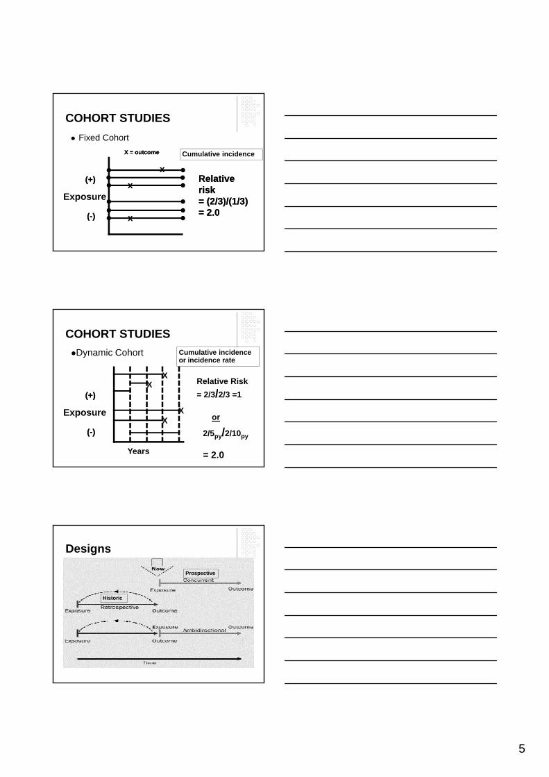
COHORT STUDIESFixed Cohort

x

X = outcomeX = outcome Cumulative incidence

Exposure

(+)(+)

((--))

x

x

Relative Relative risk risk = (= (22//33)/()/(11//33) ) = = 22..00

COHORT STUDIESDynamic Cohort

Relative RiskX

X

Cumulative incidence or incidence rate

Exposure

(+)(+)

((--))

= 2/3/2/3 =1

or

2/5py/2/10py

= 2.0Years

XX

Designs

Prospective

Historic

6

Cohort study

Prospective cohort study

Exposed

Disease

No disease

PopulationPeople without

The diseaseNot exposed Disease

Direction of the study

No disease

No disease

Follow-up is mandatory*****

Cohort study

Retrospective cohort study

Exposed

Disease

No disease

PopulationPeople without

The diseaseNot exposed Disease

Direction of the study

No disease

No disease

Cohort study

ProspectiveExposure, and factors can be measuredExpensive, time

RetrospectiveCheaperLess time consumingSuitable for rare

tconsuming outcomeSome available data is unavailable from historical partConfounding factors

7

Study designs

Example

Kidney Stone

CKD

Normal

PopulationStudy

subjectNo Stone

CKD

Direction of the study

Normal

Normal

Cohort StudyAdvantage

Can be standardized in eligible criteria & outcome assessmentCan establish temporal associationCan establish temporal association

DisadvantageUsually expensiveHard to blindLong follow-up period for rare disorderDifficult to find controls and confounders

What to look for in cohort studiesWho is at risk?

Since women who have had a bilateral mastectomy operation have almost no risk of breast cancer,17 they should not be included in cohort studies of CA breast.

Who is exposed?Cohort studies need a clear, unambiguous definition of the exposure at the outset. This definition sometimes involves quantifying the exposure by degree, rather than just yes or no.

Who is an appropriate control (the unexposed)?The key notion is that controls should be similar to the exposed in all important respects, except for the lack of exposure.

Have outcomes been assessed equally?Outcomes must be defined in advance; they should be clear, specific, and measurable.Keeping those who judge outcomes unaware of the exposure status of participants.

8

Outcome measurement (1)

Subjective outcome

Objective outcome

Fever Fever

PainPain

HemocultureHemoculture

DeathDeath

Outcome measurement (2)

Surrogate outcome

Clinical outcome

Low-density lipoprotein

(LDL)

Low-density lipoprotein

(LDL)

ProteinuriaProteinuria

DeathDeath

ESRDESRD

When should we use cohort design?

9

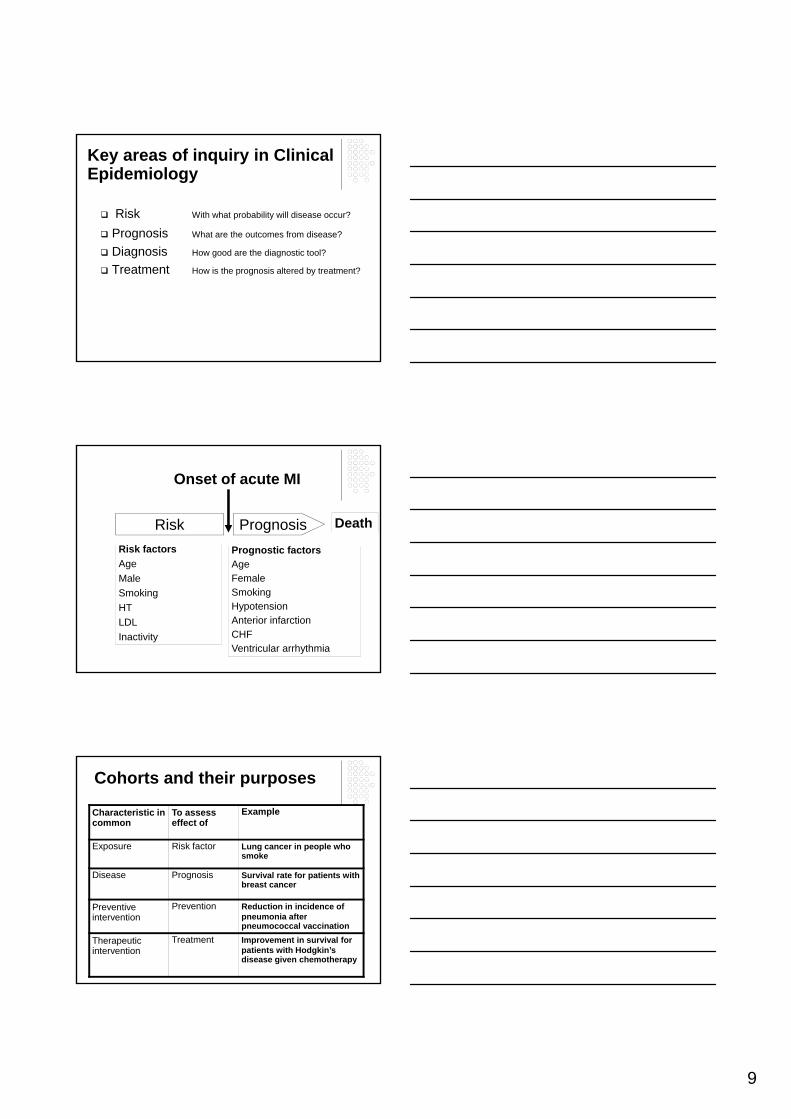
Key areas of inquiry in Clinical Epidemiology

Risk With what probability will disease occur?

Prognosis What are the outcomes from disease?

Di iDiagnosis How good are the diagnostic tool?

Treatment How is the prognosis altered by treatment?

Onset of acute MI

Risk Prognosis Death

Risk factors Prognostic factorsAgeMaleSmokingHTLDLInactivity

AgeFemaleSmokingHypotensionAnterior infarctionCHFVentricular arrhythmia

Cohorts and their purposes

Characteristic in common

To assess effect of

Example

Exposure Risk factor Lung cancer in people who smoke

Disease Prognosis Survival rate for patients with breast cancer

Preventive intervention

Prevention Reduction in incidence of pneumonia after pneumococcal vaccination

Therapeutic intervention

Treatment Improvement in survival for patients with Hodgkin’s disease given chemotherapy

10

How to assess risk or association?

Risk

The probability of some unexpected event.

The probability that people who are exposed t t i “ i k f t ” ill b tlto certain “risk factors” will subsequently develop a particular disease more often than similar people who are not exposed.

Risk factorsHypercholesterolemiaPositive family history

Valvular diseaseViral infection

SmokingDM

Multiple causes and effects

High blood pressure Congestive heart failure

Coronary atherosclerosisStroke

Renal failureMyocardial infarction

11

Way to express and compare risk

Expression Question Definition

Absolute risk What is the incidence of disease in a gr initially free of the condition?

I = #new case#People in group

Attributable risk What is the incidence of AR = IE+-IE-

(Risk difference) disease attributable to exposure?

Relative risk(Risk ratio)

How many times more likely are exposed persons to become diseased, relative to nonexposed persons?

RR = IE+

IE-

Population-attributable risk

What is the incidence of disease in a population, associated with the prevalence of a risk factor?

ARp = AR x P

Exposure

Disease No disease

Total Stone CKD No CKD

Total

+ a b a+b Yes 80 10 90- c d c+d NO 20 90 110

a+c b+d n 100 100 200

Way to express and compare risk

a+c b+d n 100 100 200Term General Example Question?

Risk a/(a+b)Or

c/(c+d)

80/90Or

20/110

What is the incidence of disease in a group initially free of the condition?

Relative risk a/(a+b) ÷c/(c+d)

80/90 ÷ 20/110= 5

How many times more likely are exposed persons to become disease, relative to nonexposed persons?

Exposure

Disease No disease

Total Stone CKD No CKD

Total

+ a b a+b Yes 80 10 90- c d c+d NO 20 90 110

Way to express and compare risk

a+c b+d n 100 100 200Term General Example Definition

Attributable risk (AR)

a/(a+b) –c/(c+d)

80/90 – 20/110= 0.7

The incidence of disease attributable to exposure

Population attributable riskPAR= ARxPEX

AR x (a+b)/n

0.7 x 90/200= 0.32

The incidence of disease in a population is associated with the occurrence of a risk factor

12

Relative risk vs. attributable risk

RR The strength of associationCausal inference

ARMeasure of how much of the disease risk is attributable to a certain Causal inference

Valuable in etiologic studies

exposureValuable in clinical practice and public health

Incidence

Ipop - I unexposed

Population attributable risk (PAR)

population unexposed

PAR% = {(Ipop - I unexposed ) / Ipop}100

Incidence

Ipop - I unexposed

Population attributable risk (PAR)If we had an effective prevention program (stop stone) in this population, how much of a reduction in CKD incidence could we

ti i t i th t t l

population unexposed

PAR% = {(Ipop - I unexposed ) / Ipop}100

anticipate in the total population (of both stones and no stones)?

13

Incidence rate

The measure of disease in cohort studies is the incidence rate, which is the proportion of subjects who develop the disease under study within a specified time periodstudy within a specified time period. The numerator of the rate is the number of diseased subjects.the denominator is usually the number of person-years of observation.

Total observed person-time 69.1 mo.

Survival analysisThe likelihood that patients with a given condition will experience an outcome at any point in time.Cohort or a randomized control trialCohort or a randomized control trialTime to event

Origin End point

14

Why survival analysis?Investigators Frequently must analyze their data before all the subjects have died or the event has occurred.

Why survival analysis?Investigators frequently must analyze their data before all the subjects have died or the event has occurred.The patients do not typically enter theThe patients do not typically enter the study at the same time.

Total observed person-time 69.1 mo.

15

Survival analysisEvent : Code 1 0

1= Event occurred : death0= censored observation: alive or0= censored observation: alive or

loss to follow-upCensored observation: An observation whose value is unknown because the subject has not been in the study long enough for the outcome of interest to occur

Methodological characteristics of survival study

The starting date for each patient must clearly defined

date of diagnosedate of receiving treatmentdate of operation, etc.

The end date for each patient Patient’s status at the end

Death if death is the final outcome recurrence, disease free infection, non-infection remission, non-remission recovery, non-recovery loss to follow up, withdraw

Survival Probability

The proportion of population of such people who survive a given length of time in the same circumstances. An estimate of survivorship function S(t)An estimate of survivorship function S(t) is the estimated proportion of individual who survive longer than time

-(1)----- sindividual ofnumber Total

t thanlonger survive who sindividual ofNumber =∧

)(tS

16

Life table analysis

ni wi di qi=di/[ni-(wi/2)]

Pi=1-qi Si=pi(pi-1)

Interval start time(mo)

No entering this interval

No withdrawal during

No of terminal events

Proportion terminating

Proportion surviving

Cum proportion surviving at ( )

interval End

0 13 2 1 0.083 0.917 0.917

3 10 4 1 0.125 0.875 0.802

6 5 4 0 0 1.000 0.802

9 1 1 0 0 1.000 0.802

Kaplan-Meier method ni Ci di qi= di/ni Pi=1-qi Si=pi(pi-1)

Event time(mo)

No at risk Censor No of events

Mortality Survival Cum survival

3 10 0 1 1/10=0.1 0.90 0.9

4 9 1 0 0/9=0 1.0 0.9*1=0.9

5.7 8 1 0 0/8=0 1.0 0.9*1*1=0.9

6.5 7 0 2 2/7= 0.28 0.72 0.9*1*1*0.72=0.648

.

10

Kaplan-Meier survival estimate

1 1

1

100.

751.

00ob

abili

ty

Figure 3. Kaplan-Meier survival estimate with censoring

1

0.00

0.25

0.50

Sur

viva

l pro

0 2 4 6 8 10 12 14Time (months)

17

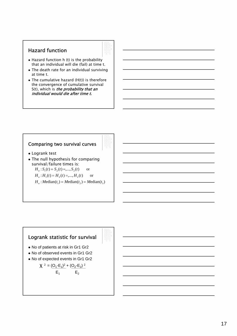
Hazard function

Hazard function h (t) is the probability that an individual will die (fail) at time t.The death rate for an individual surviving at time tat time t. The cumulative hazard (H(t)) is therefore the convergence of cumulative survival S(t), which is the probability that an individual would die after time t.

Comparing two survival curves

Logrank testThe null hypothesis for comparing survival/failure times is:

)()()( SSSH

)(edian)(edian)(edian :or )(,...,)()( :

or )(,..., )()( :

321

221

221

tMtMtMHtHtHtHH

tStStSH

o

o

o

====

==

Logrank statistic for survival

No of patients at risk in Gr1 Gr2No of observed events in Gr1 Gr2No of expected events in Gr1 Gr2χ 2 = (O1-E1)2 + (O2-E2) 2

E1 E2

18

Time(month)

d1jNumber ofDeaths

n1jNumber at risk

d2j n2j dj nj e1j e2j

.03

.07.1

.17

.23

.27

.50

1111111

1514131211109

0000000

15151515151515

1111111

30292827262524

1x15/30=.501x14/29=.481x13/28=.46

.44

.42

.40

.38

1x15/30=.501x15/29=.521x15/28=.54

.56

.57

.60

.63

j

jj

ndn 1

=j

jj

ndn 2

=

Demonstrating calculation of Log-rank statistics

3.035.939.139.80

13.2315.83

101100

877655

010011

151514141413

111111

232221201918

.35

.32

.33

.30

.26

.28

.65

.68

.67

.70

.74

.72

Total 10O1

3O2

4.93E1

8.07E2

39.807.8

)07.83(93.4

)93.410( 222

=

−+

−=χ

P=0.001

Hazard ratioHR = O1/E1

O2/E2

= 10/4.93 = 2.03/0.37 = 5.53/8.07

The risk of GF at any time in recipients olderthan 50 years old is 5.5 times greater than the riskin recipients who younger.

Faster

stsum, by(ager_gr)failure _d: GF == 1

analysis time _t: _tid: hnr

| incidence no. of |------ Survival time -----|ager_gr | time at risk rate subjects 25% 50% 75%---------+---------------------------------------------------------------------

<50 | 831.5701574 .0865832 253 3.756331 6.652977 .>=50 | 229.7221081 .0740025 71 3.635866 . .

---------+---------------------------------------------------------------------total | 1061.292266 .08386 324 3.635866 . .

. sts test ager_grfailure d: GF == 1

CC-EBM

failure _d: GF == 1analysis time _t: _t

id: hnr

Log-rank test for equality of survivor functions

| Events Eventsager_gr | observed expected--------+-------------------------<50 | 72 69.61>=50 | 17 19.39--------+-------------------------Total | 89 89.00

chi2(1) = 0.38Pr>chi2 = 0.5391

19

Statistical analysisSurvival analysis with Kaplan-Meier was used to estimate survival rate, median survival time of recipients. Log-rank test was used to compare survival g pcurves Cox regression was used to determine factors associated with survival time

Cox regressionProportional hazard model

The Cox proportional hazard model (or Cox regression) was proposed by Cox in 1972 and has been used widely since then when desiring to investigate several variables simultaneously for time to event outcomes. The model is a semi-parametric approach –no particular type of distribution is assumed for survival times.

Cox regressionProportional hazard model

A strong assumptionThe effects of the different groups of variable on survival are constant over timetime.

Benefits of the Cox model are: (i) It can perform multiple comparisons (ii) It’s able to adjust for confounding variables for which the study design can not control for.

20

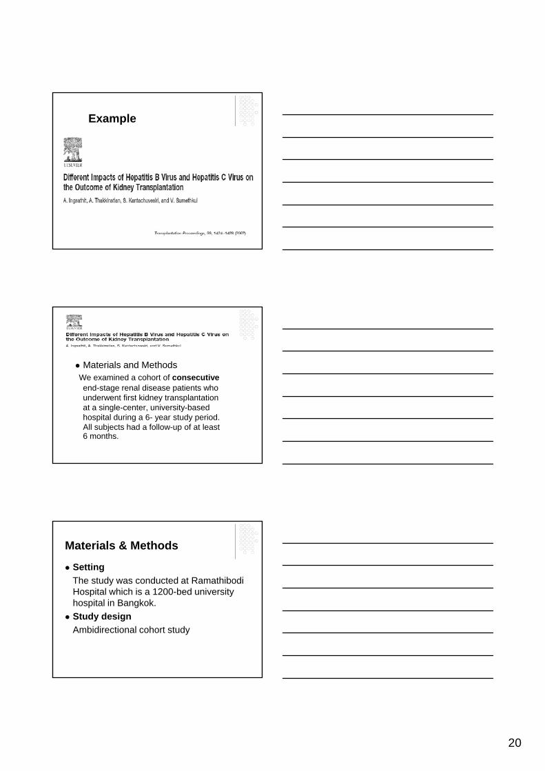
Example

Materials and Methods We examined a cohort of consecutive

d t l di ti t hend-stage renal disease patients who underwent first kidney transplantation at a single-center, university-based hospital during a 6- year study period. All subjects had a follow-up of at least 6 months.

Materials & Methods

SettingThe study was conducted at Ramathibodi Hospital which is a 1200-bed university hospital in Bangkok.Study designAmbidirectional cohort study

21

MethodsStudy design

A ambidirectional cohort studyPast Present Future

Start 1997 2002 2006

Materials & MethodsStudy population

Inclusion criteriaMedical records of patients aged at least 18 years

old who initially had undertaken kidney transplantation inold who initially had undertaken kidney transplantation in Ramathibodi Hospital

Exclusion criteriaMulti-organ transplants or dual kidney transplantsRecipient who had graft failure or death within 6 monthsRecipients who had time of follow-up of less than 6 months

Study design

HBV HCVHBV

HCV

GF

No GF

GFHCV

Non HBVHCV

Follow over time

No GF

GF

No GF

22

OutcomeThe primary outcomes were time to graft failure.

Graft failure was defined by the introductionGraft failure was defined by the introduction of long-term dialysis after transplantation or retransplantation.

Statistical analysisGraft and patient and survivals were determined using the Kaplan-Meier method.

Log-rank test was used to compare survival curvessurvival curves Cox regression analysis with time-varying covariates was used to assess the effect of HBV/HCV infections adjusting for confounders.

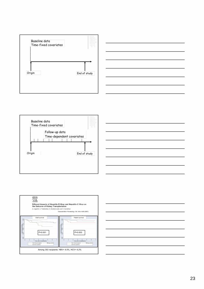
Data collection

Baseline dataFollow-up data

23

Baseline dataTime-fixed covariates

Origin End of study

Baseline dataTime-fixed covariates

Follow-up dataTime-dependent covariates

Origin End of study

.75

1.00

y

Composite survival

.75

1.00

y

Patient survivalGraft survival Patient survival

0.00

0.25

0.50

0Su

rviv

al p

roba

bilit y

0 1 2 3 4 5 6 7Years post transplantation

Non inf ected patient HBsAg positiv eAnti-HCV positiv e

0.00

0.25

0.50

0Su

rviv

al p

roba

bilit y

0 1 2 3 4 5 6 7Years post transplantation

Non inf ected patient HBsAg positiv eAnti-HCV positiv e

P=0.001 P=0.003

Among 353 recipients: HBV+ 6.5%, HCV+ 6.2%

24

Incidence of graft failure and HR

Characteristics No. ofGF

Totalsubjects

Timeat risk(years)

IncidenceGF/100/year

Hazard ratio(95%CI)

P-value

Recipient age, years < 50 > 50

920

26477

272.56981.12

3.302.01

1.0***1.67(0.76-3.68)

0.20

Sex 0 84SexMaleFemale

1019

131210

461.93791.75

2.162.40

1.0***1.10(0.50-2.33)

0.84

Duration of dialysis <12 months

>12 months 1415

162161

623.69551.88

2.242.71

1.0***1.17(0.56-2.43)

0.66

Anti-HCVPositiveNegative 6

2322319

90.331171.7

7.331.96

3.88(1.57-9.57)1.0***

0.001

Potential bias in cohort studies

Selection bias Susceptibility biasMigration biasMigration bias

Measurement biasSurvival cohortsConfounders

Selection or Susceptibility bias

Groups being compared are not equally susceptible to the outcome of interest, other than the factor under studyCCA colon : CEA level and Relapse

Dukes classification and Relapse

25

Methods for controlling selection bias

MethodPhase of study

Design Analysis

Randomization +

Restriction +

Matching +

Stratification +

AdjustmentMultivariable

+

Migration bias

HBV HCVHBV

HCV

GF

No GF

GF

Drop out

HCV

Non HBVHCVFollow over time

No GF

GF

No GF

Cross over

Best-case/worst case analysis

Measurement bias

When patients in one subgroup of a cohort stand a better chance of having their outcomes detected than another subgroup.Ways to controlWays to control

Unawareness of person who record outcome eventsSet up strict criteria/rules for diagnose outcome eventsApply efforts to discover outcome events equally

26

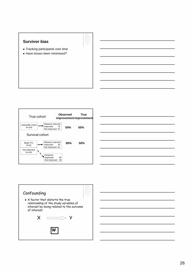
Survivor bias

Tracking participants over timeHave losses been minimised?

True cohort Observed improvement

True improvement

Assemble cohortN=150

Measure outcomeImproved: 75Not improved: 75 50% 50%

Survival cohort

Begin F/UN=50

Not observedN=100

Measure outcomeImproved: 40Not improved: 10

DropoutsImproved: 35Not improved: 65

80% 50%

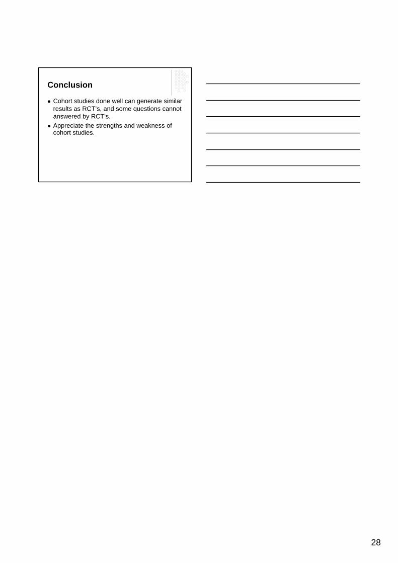
ConfoundingA factor that distorts the true relationship of the study variables of interest by being related to the outcome of interest.

X Y

W

27

ConfoundingIt must be a risk factor for outcome It must be associated with the exposure or distributed unequallyunequally between the groups

Exposure

(Coffee drinking)

Outcome

(CA stomach)

ConfoundingIt must be a risk factor for outcome It must be associated with the exposure or distributed unequallyunequally between the groups

Exposure

(Coffee drinking)

Outcome

(CA stomach)

Confounding variable

(Smoking)

Features to look for in a cohort study

28

Conclusion

Cohort studies done well can generate similar results as RCT’s, and some questions cannot answered by RCT’s.Appreciate the strengths and weakness ofAppreciate the strengths and weakness of cohort studies.