Wireless Pers Commun (2015) 82:1623–1642DOI 10.1007/s11277-015-2303-8

Coherent Detection of Turbo-Coded OFDM SignalsTransmitted Through Frequency Selective RayleighFading Channels with Receiver Diversity and IncreasedThroughput

K. Vasudevan

Published online: 3 February 2015© The Author(s) 2015. This article is published with open access at Springerlink.com

Abstract In this work, we discuss techniques for coherently detecting turbo coded orthogo-nal frequency division multiplexed (OFDM) signals, transmitted through frequency selectiveRayleigh (the magnitude of each channel tap is Rayleigh distributed) fading channels havinga uniform power delay profile. The channel output is further distorted by a carrier frequencyand phase offset, besides additive white Gaussian noise. A new frame structure for OFDM,consisting of a known preamble, cyclic prefix, data and known postamble is proposed, whichhas a higher throughput compared to the earlier work. A robust turbo decoder is proposed,which functions effectively over a wide range of signal-to-noise ratio (SNR). Simulationresults show that it is possible to achieve a bit-error-rate (BER) of 10−5 at an SNR per bitas low as 8dB and throughput of 82.84%, using a single transmit and two receive antennas.We also demonstrate that the practical coherent receiver requires just about 1dB more powercompared to that of an ideal coherent receiver, to attain a BER of 10−5. The key contributionto the good performance of the practical coherent receiver is due to the use of a long preamble(512 QPSK symbols), which is perhaps not specified in any of the current wireless communi-cation standards. We have also shown from computer simulations that, it is possible to obtaineven better BER performance, using a better code. A simple and approximate Cramér–Raobound on the variance of the frequency offset estimation error for coherent detection, isderived. The proposed algorithms are well suited for implementation on a DSP-platform.

Keywords OFDM · Coherent detection · Matched filtering · Turbo codes · Frequencyselective Rayleigh fading · Channel capacity

This work is supported by the India-UK Advanced Technology Center (IU-ATC) of Excellence in NextGeneration Networks, Systems and Services under grant SR/RCUK-DST/IUATC Phase 2/2012-IIT K (C),sponsored by DST-EPSRC. This work was partly presented as an Invited Talk at the International Federationof Nonlinear Analysts (IFNA) World Congress, Greece, June 2012 and partly published in ISPCC, Sept.2013, Shimla and ITST Nov. 2013, Finland.

K. Vasudevan (B)Department of EE, IIT Kanpur, Kanpur, Indiae-mail: vasu@iitk.ac.in

123

1624 K. Vasudevan

1 Introduction

Future wireless communication standards aim to push the existing data-rates higher. Thiscan only be achieved with the help of coherent communications, since they give the lowestbit-error-rate (BER) performance for a given signal-to-noise ratio (SNR). Conversely, theyrequire the lowest SNR to attain a given BER, resulting in enhanced battery life. If we lookat a mobile, it indicates a typical received signal strength equal to −100dBm (10−10 mW).However this is not the signal-to-noise ratio! Therefore, the question is:What is the operatingSNR of the mobiles? Would it be possible to achieve the same performance by transmittingat a lower power? The recent advances in cooperative communications has resulted in lowcomplexity solutions, that are not necessarily power efficient [1,2]. In fact, it is worth quotingthe following from [3]:

1. The Myth: Sixty years of research following Shannon’s pioneering paper has ledto telecommunications solutions operating arbitrarily close to the channel capacity—“flawless telepresence” with zero error is available to anyone, anywhere, anytime acrossthe globe.

2. The Reality: Once we leave home or the office, even top of the range iPhones and tabletcomputers fail to maintain “flawless telepresence” quality. They also fail to approach thetheoretical performance predictions. The 1,000-fold throughput increase of the best third-generation (3G) phones over second-generation (2G) GSM phones and the 1,000-foldincreased teletraffic predictions of the next decade require substantial further bandwidthexpansion toward ever increasing carrier frequencies, expanding beyond the radio- fre-quency (RF) band to optical frequencies, where substantial bandwidths are available.

The transmitter and receiver algorithms proposed in this paper and in [4,5] are well suitedfor implementation on a DSP processor or hardwired and may perhaps not require quantumcomputers, asmentioned in [3]. The reader is also referred to the brief commentary on channelestimation and synchronization in page 1351 and also to the noncoherent schemes in page1353 of [1], which clearly state that cooperative communications avoid coherent receiversdue to complexity.

Broadly speaking, thewireless communicationdevice needs to have the following features:

1. maximize the bit-rate2. minimize the bit-error-rate3. minimize transmit power4. minimize transmission bandwidth

A rather disturbing trend in the present day wireless communication systems is to make thephysical layer very simple and implement it in hardware, and allot most of the computingresources to the application layer, e.g., for internet surfing, video conferencing etc. Whilehardware implementation of the physical layer is not an issue, in fact, it may even be preferredover software implementation in some situations, the real cause for concern is the tendencyto make it “simple”, at the cost of BER performance. Therefore, the questions are:

1. was signal processing for coherent communications given a chance to prove itself, orwas it ignored straightaway, due to “complexity” reasons?

2. are the present day single antenna wireless transceivers, let alone multi-antenna systems,performing anywhere near channel capacity?

This paper demonstrates that coherent receivers need not be restricted to textbooks alone, infact they can be implemented with linear (not exponential) complexity. The need of the houris a paradigm shift in the way the wireless communication systems are implemented.

123

Frequency Selective Rayleigh Fading Channels 1625

In this article, we dwell on coherent receivers based on orthogonal frequency divisionmultiplexing (OFDM), since it has the ability to mitigate intersymbol interference (ISI)introduced by the frequency selective fading channel [6–8]. The “complexity” of coherentdetection can be overcome by means of parallel processing, for which there is a large scope.We wish to emphasize that this article presents a proof-of-concept, and is hence not con-strained by the existing standards in wireless communication. We begin by first outlining thetasks of a coherent receiver. Next, we scan the literature on each of these tasks to find out thestate-of-the-art, and finally end this section with our contributions.

The basic tasks of the coherent receiver would be:

1. To correctly identify the start of the (OFDM) frame (SoF), such that the probability of falsealarm (detecting an OFDM frame when it is not present) or equivalently the probabilityof erasure/miss (not detecting the OFDM frame when it is present) is minimized. Werefer to this step as timing synchronization.

2. To estimate and compensate the carrier frequency offset (CFO), since OFDM is knownto be sensitive to CFO. This task is referred to as carrier synchronization.

3. To estimate the channel impulse/frequency response.4. To perform (coherent) turbo decoding and recover the data.

To summarize, a coherent receiver at the physical layer ensures that the medium accesscontrol (MAC) is not burdened by frequent requests for retransmissions.

A robust timing and frequency synchronization for OFDM signals transmitted throughfrequency selective additive white Gaussian noise (AWGN) channels is presented in [9].Timing synchronization in OFDM is addressed in [10–14]. Various methods of carrier fre-quency synchronization for OFDM are given in [15–21]. Joint timing and CFO estimation isdiscussed in [22–27].

Decision directed coherent detection of OFDM in the presence of Rayleigh fading istreated in [28]. A factor graph approach to the iterative (coherent) detection of OFDM inthe presence of CFO and phase noise is presented in [29]. OFDM detection in the presenceof intercarrier interference (ICI) using block whitening is discussed in [30]. In [31], a turboreceiver is proposed for detecting OFDM signals in the presence of ICI and inter antennainterference.

Most flavors of the channel estimation techniques discussed in the literature are done inthe frequency domain, using pilot symbols at regular intervals in the time/frequency grid [32–36]. Iterative joint channel estimation and multi-user detection for multi-antenna OFDM isdiscussed in [37]. Noncoherent detection of coded OFDM in the absence of frequency offsetand assuming that the channel frequency response to be constant over a block of symbols,is considered in [38]. Expectation maximization (EM)-based joint channel estimation andexploitation of the diversity gain from IQ imbalances is addressed in [39].

Detection of OFDM signals, in the context of spectrum sensing for cognitive radio, isconsidered in [40,41]. However, in both these papers, the probability of false alarm is quitehigh (5%).

In [42], discrete cosine transform (DCT) based OFDM is studied in the presence of fre-quency offset and noise, and its performance is compared with the discrete Fourier transform(DFT) based OFDM. It is further shown in [42] that the performance of DFT-OFDM is asgood as DCT-OFDM, for small frequency offsets.

A low-power OFDM implementation for wireless local area networks (WLANs) isaddressed in [43]. OFDM is a suggested modulation technique for digital video broadcasting[44,45]. It has also been proposed for optical communications [46].

123

1626 K. Vasudevan

The novelty of this work lies in the use of a filter that is matched to the preamble, to acquiretiming synchronization [47,48] (start-of-frame (SoF) detection). Maximum likelihood (ML)channel estimation using the preamble is performed. This approach does not require anyknowledge of the channel and noise statistics.

The main contributions of this paper are the following:

1. It is shown that, for a sufficiently long preamble, the variance of the channel estimatorproposed in eq. (28) of [4] approaches zero.

2. A known postamble is used to accurately estimate the residual frequency offset for largedata lengths, thereby increasing the throughput compared to [4,5].

3. Turbo codes are used to attain BER performance closer to channel capacity compared toany other earlier work in the open literature, for channels having a uniform power delayprofile (to the best of the authors knowledge, there is no similar work on the topic of thispaper, other than [4,5]).

4. A robust turbo decoder is proposed, which performs effectively over a wide range ofSNR (0–30dB).

In a multiuser scenario, the suggested technique is OFDM-TDMA. The uplink and downlinkmay be implemented using time division duplex (TDD) or frequency division duplex (FDD)modes.

This paper is organized as follows. Section 2 describes the system model. The enhancedframe structure is described in Sect. 3. The modifications in the turbo decoder in the presenceof receive diversity and the variance of the channel estimation error, are presented in Sect. 4.The channel capacity is discussed in Sect. 5. The BER results from computer simulations aregiven in Sect. 6. Finally, in Sect. 7, we discuss the conclusions and future work.

2 System Model

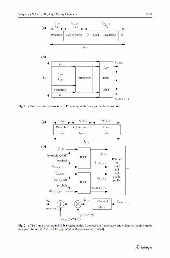
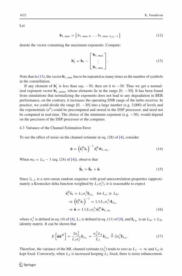
We assume 1st-order transmit diversity and N th-order receive diversity. The data is orga-nized into frames, as depicted in Fig. 1. The earlier frame structure considered in [4] is givenin Fig. 2.

The received signal in each diversity arm (l) can be expressed as (see also eq. (5) in [4]):

rk, n, l =(sk, n � hk, n, l

)e j(ωkn+θk, l ) + wk, n, l

= yk, n, lej(ωkn+θk, l ) + wk, n, l (1)

for 1 ≤ l ≤ N . The frequency offset is assumed to be identical for all the diversity arms,whereas the carrier phase and noise are assumed to be independent. The noise variance issame for all the diversity arms. Two extreme scenarios are considered in the simulations (a)identical channel and (b) independent channel in each diversity arm. The channel span is Lh

and is assumed to have a uniform power delay profile.The output of the FFT can be written as (for 0 ≤ i ≤ Ld − 1):

Rk, i, l = Hk, i, l Sk, 3, i + Wk, i, l (2)

for 1 ≤ l ≤ N diversity arms. The notation in (2) is self explanatory and is based on eq. (36)in [4].

123

Frequency Selective Rayleigh Fading Channels 1627

(a)

(b)

Ld

Postamble

Interleaver

Ld−

point

IFFT

sk, 3,L d−1

sk, 3, 0

Lp

s1,n

Lcp

sk, 2,n

Ld

sk, 3,n

Preamble

sk,n

Cyclic prefix B Data Postamble B

B

B

Data

Ld2

Fig. 1 a Enhanced frame structure. b Processing of the data part at the transmitter

IFFT

IFFT

ChannelTo

receiver

Preamble QPSK

symbols

Data QPSK

symbols

sk,n

hk,n

wk,n (AWGN)

(a)

(b)

e j(ωkn+θk)

Lp

ataDelbmaerP

LdLcp

sk, 2,n sk, 3,n

sk,n

Cyclic prefix

s1,n

S1, 0

S1,Lp−1

Sk, 3, 0

Sk, 3,Ld−1

s1, 0

s1,Lp−1

sk, 3, 0

sk, 3,Ld−1

yk,n

to

andadd

cyclicprefix

Parallel

serial

Fig. 2 a The frame structure in [4]. b System model. k denotes the frame index and n denotes the time indexin a given frame. © 2013 IEEE. Reprinted, with permission, from [4]

123

1628 K. Vasudevan

1.0e-05

1.0e-04

1.0e-03

1.0e-02

1.0e-01

0 2 4 6 8 10 12

RMS coarseRMS fine

Max coarseMax fine

RMS cohoApprox CRB

SNR per bit (dB)

Freq

off

set e

st e

rror

(rad

ians

)

Fig. 3 RMS and maximum frequency offset estimation error for L p = 512

3 Enhanced Frame Structure

The basic motivation behind the enhanced frame structure, is to increase the throughput,which in turn, depends on Ld . The accuracy of the frequency offset estimate depends onthe length of the preamble L p . Increasing the number of frequency bins B1 and B2 [4] for agiven L p , does not improve the accuracy. From Fig. 3 it can be seen that the RMS value ofthe fine frequency offset estimation error is about 2× 10−4, at an SNR per bit equal to 8dB.The subcarrier spacing with data length Ld = 4,096 is equal to 2π/4,096 = 1.534 × 10−3

radians. Therefore, the residual frequency offset is 0.0002 × 100/0.001534 = 13% of thesubcarrier spacing, which is quite high and causes severe ICI. Note that the RMS frequencyoffset estimation error can be reduced by increasing the preamble length (L p), keeping thedata length (Ld ) fixed, which in turn reduces the throughput given by (for the frame structurein Fig. 2):

T = Ld1

L p + Lcp + Ld(3)

where Ld1 is defined in Fig. 4, for the frame structure given in Fig. 2. Note that for a rate-1/2turbo code Ld = 2Ld1, whereas for a rate-1 turbo code, Ld = Ld1. This motivates us tolook for an alternate frame structure which not only solves the frequency offset estimationproblem, but also maintains the throughput at a reasonable value.

Consider the frame in Fig. 1a. In addition to the preamble, prefix and data, it contains“buffer” (dummy) symbols of length B and postamble of length Lo, all drawn from theQPSK constellation. In Fig. 1b we illustrate the processing of Ld symbols at the transmitter.Observe that only the data and postamble symbols are interleaved before the IFFT operation.After interleaving, the postamble gets randomly dispersed between the data symbols. Thebuffer symbols are sent directly to the IFFT, without interleaving. The preamble and thecyclic prefix continue to be processed according to Figure 1 in [4] and eq. (3) in [4]. We nowexplain the reason behind using this frame structure. In what follows, we assume that theSoF has been detected, fine frequency offset correction has been performed and the channelhas been estimated.

123

Frequency Selective Rayleigh Fading Channels 1629

Fig. 4 Encoder block diagramfor the frame structure in Fig. 2.© 2013 IEEE. Reprinted, withpermission, from [4]

to

QPSK

Map

Map

to

QPSK

Input

bitslength Ld1

Rate-1/2RSC

Rate-1/2RSC

encoder 1

encoder 2

Encoder 1QPSK symbols

length Ld1

QPSK symbolslength Ld1

Encoder 2

Total length Ld = 2Ld1

Interleaver

(π)

We proceed by making the following observations:

1. Modulation in the time domain results in a shift in the frequency domain. Therefore,any residual frequency offset after fine frequency offset correction, results in a frequencyshift at the output of the FFT operation at the receiver. Moreover, due to the presence of acyclic prefix, the frequency shift is circular. Therefore, without the buffer symbols, thereis a possibility that the first data symbol would be circularly shifted to the last data symbolor vice versa. This explains the use of buffer symbols at both ends in Fig. 1. In orderto compute the number of buffer symbols (B), we have to know the maximum residualfrequency offset, after fine frequency offset correction. Referring to Fig. 3,we find that themaximum error in fine frequency offset estimation at 0dB SNRper bit is about±2×10−3

radians. With Ld = 4,096, the subcarrier spacing is 2π/4,096 = 1.534× 10−3 radians.Hence, the residual frequency errorwould result in a shift of±2/1.534 = ±1.3 subcarrierspacings. Therefore, while B = 2 would suffice, we have taken B = 4, to be on the safeside.

2. Since the frequency shift is not an integer multiple of the subcarrier spacing, we needto interpolate in between the subcarriers, to accurately estimate the shift. Interpolationcan be achieved by zero-padding the data before the FFT operation. Thus we get a2Ld−point FFT corresponding to an interpolation factor of two and so on. Othermethodsof interpolation between subcarriers is discussed in [49].

3. After the FFT operation, postamble matched filtering has to be done, since the postam-ble and Hk ≈ Hk are known. The procedure for constructing the postamble matchedfilter is illustrated in Fig. 5. From simulations, it has been found that a postamble lengthLo = 128 results in false peaks at the postamble matched filter output at 0dB SNRper bit. Therefore we have taken Lo = 256. With these calculations, the length ofthe data works out as Ld2 = Ld − 2B − Lo = 4,096 − 8 − 256 = 3,832 QPSKsymbols. The throughput of the enhanced frame structure (with rate-1 turbo code)is

123

1630 K. Vasudevan

Fig. 5 Obtaining the postamblematched filter for Ld = 8. Buffersymbols are not shown. Thefrequency offset (π/Ld ) is halfthe subcarrier spacing (2π/Ld ).Hk and Sk are assumed to bereal-valued. Noise is absent. aOutput of the Ld -point FFT inthe absence of frequency offset.The red lines represent postambleand the blue lines represent datasymbols. b Output of the2Ld -point FFT in the presence offrequency offset. Observe that thered and blue lines have shifted tothe right by π/Ld . Green linesdenote the output of the Ld -pointFFT in the presence of frequencyoffset. c The postamble matchedfilter

HkSk

k

(a)

0 15

HkSk

k

(b)

0 15

k

(c)HkSk

0

7

Table 1 Throughput comparison of various frame structures with L p = Ld1 = 512, Ld2 = 3,832, Lcp = 18

Frame structure in Fig. 2rate-1/2 turbocode [4] Eq. (3)

Frame structure in Fig. 2rate-1 turbocode [5] Eq. (3)

Frame structure in Fig. 1rate-1 turbo code(proposed) Eq. (4)

Throughput(%)

32.95 49.14 82.84

T = Ld2

L p + Lcp + Ld

= 3,832

512 + 18 + 4,096= 82.84%. (4)

The throughput comparison of various frame structures is summarized in Table 1.

4 Receiver

The receiver algorithms for start-of-frame (SoF) detection, frequency offset, channel andnoise variance estimation are already discussed in [4,5], and apply also to the enhanced framestructure given above and receive diversity. In what follows, we describe the modificationsrequired in the turbo decoder in the presence of receive diversity.

4.1 Turbo Decoding

In the turbo decoding operation, (for decoder 1, transition from state m to n, kth frame, Ndiversity arms, rate-1/2 turbo code, the enhanced frame structure in Fig. 1 and 0 ≤ i ≤

123

Frequency Selective Rayleigh Fading Channels 1631

Ld2/2 − 1), we have (assuming independent noise in all the diversity arms)

γ1, k, i,m, n =N∏l=1

γ1, k, i,m, n, l (5)

where

γ1, k, i,m, n, l = exp

⎡⎢⎣−

(Rk, i, l − Hk, i, l Sm, n

)2

2Ld σ 2w

⎤⎥⎦ (6)

where σ 2w is the average estimate of the noise variance over all the diversity arms and Sm, n

is the QPSK symbol corresponding to the transition from state m to n.Similarly at decoder 2, for 0 ≤ i ≤ Ld2/2 − 1, we have:

γ2, k, i,m, n =N∏l=1

γ2, k, i,m, n, l (7)

where

γ2, k, i,m, n, l = exp

⎡⎢⎣−

(Rk, j, l − Hk, j, l Sm, n

)2

2Ld σ 2w

⎤⎥⎦ (8)

where

j = Ld3 + i

Ld3 = Ld2/2. (9)

For a rate-1 turbo code obtained by puncturing, alternate gammas have to be set to unity[5,7]. The rest of the BCJR algorithm is described in [5,7].

4.2 Robust Turbo Decoding

At high SNR, the term in the exponent (b is the exponent of eb) of (6) and (8) becomes verylarge (typically b > 100) and it becomes unfeasible for the DSP processor or even a computerto calculate the gammas. We propose to solve this problem by normalizing the exponents.Observe that the exponents are real-valued and negative. Let b1, j, i denote an exponent atdecoder 1 due to the j th symbol in the constellation (1 ≤ j ≤ 4 for QPSK) at time i . Fornotational convenience, we again assume a rate-1/2 turbo code. Let

b1 =⎡⎢⎣b1, 1, 0 . . . b1, 1, Ld3−1

......

...

b1, 4, 0 . . . b1, 4, Ld3−1

⎤⎥⎦ (10)

denote the matrix of exponents for decoder 1. Let b1,max, i denote the maximum exponent attime i , that is

b1,max, i = max

⎡⎢⎣b1, 1, i

...

b1, 4, i

⎤⎥⎦ . (11)

123

1632 K. Vasudevan

Let

b1,max = [b1,max, 0 . . . b1,max, Ld3−1

](12)

denote the vector containing the maximum exponents. Compute:

b′1 = b1 −

⎡⎢⎣b1,max

...

b1,max

⎤⎥⎦ . (13)

Note that in (13), the vector b1,max has to be repeated asmany times as the number of symbolsin the constellation.

If any element of b′1 is less than say, −30, then set it to −30. Thus we get a normal-

ized exponent vector b1, norm, whose elements lie in the range [0, −30]. It has been foundfrom simulations that normalizing the exponents does not lead to any degradation in BERperformance, on the contrary, it increases the operating SNR range of the turbo receiver. Inpractice, we could divide the range [0, −30] into a large number (e.g. 3,000) of levels andthe exponentials (eb) could be precomputed and stored in the DSP processor, and need notbe computed in real-time. The choice of the minimum exponent (e.g. −30), would dependon the precision of the DSP processor or the computer.

4.3 Variance of the Channel Estimation Error

To see the effect of noise on the channel estimate in eq. (28) of [4], consider

u =(sH1 s1

)−1sH1 wk,m1 . (14)

When m0 = Lh − 1 (eq. (24) of [4]), observe that

hk = hk + u. (15)

Since s1, n is a zero-mean random sequence with good autocorrelation properties (approxi-mately a Kronecker delta function weighted by L1σ

2s ), it is reasonable to expect

sH1 s1 = L1σ2s ILhr for L p � Lhr

⇒(sH1 s1

)−1 = 1/(L1σ2s )ILhr

⇒ u = 1/(L1σ2s )sH1 wk,m1 (16)

where σ 2s is defined in eq. (4) of [4], L1 is defined in eq. (11) of [4], and ILhr is an Lhr × Lhr

identity matrix. It can be shown that

E[uuH

]= 2σ 2

w

L1σ 2sILhr = σ 2

wLd

L1ILhr

�= 2σ 2u ILhr . (17)

Therefore, the variance of the ML channel estimate (σ 2u ) tends to zero as L1 → ∞ and Ld is

kept fixed. Conversely, when Ld is increased keeping L1 fixed, there is noise enhancement.

123

Frequency Selective Rayleigh Fading Channels 1633

5 The Channel Capacity

The communication system model under consideration is given by (2). The channel capacityis given by [50]:

C = 1

2log2(1 + SNR) bits/transmission (18)

per dimension (real-valued signals occupy a single dimension, complex-valued signalsoccupy two dimensions). The “SNR” in (18) denotes the minimum average signal-to-noiseratio per dimension, for error-free transmission. Observe that:

1. The sphere packing derivation of the channel capacity formula [50], does not require noiseto be Gaussian. The only requirements are that the noise samples have to be independent,the signal and noise have to be independent, and both the signal and noise must have zeromean.

2. The channel capacity depends only on the SNR.3. The average SNR per dimension in (18) is different from the average SNR per bit (or

Eb/N0), which is widely used in the literature. In fact, it can be shown that [7,50]:

SNR = 2C × SNR per bit. (19)

4. It is customary to define the average SNR per bit (Eb/N0) over two dimensions (complexsignals). When the signal and noise statistics over both dimensions are identical, theaverage SNR per bit over two dimensions is identical to the average SNR per bit over onedimension. Therefore (19) is valid, even though the SNR is defined over one dimensionand the SNR per bit is defined over two dimensions.

5. The notation Eb/N0 is usually used for continuous-time, passband analog signals [50–52], whereas SNR per bit is used for discrete-time signals [7]. However, both definitionsare equivalent. Note that passband signals are capable of carrying information over twodimensions, using sine and cosine carriers, inspite of the fact that passband signals arereal-valued.

6. Each dimension corresponds to a separate and independent path between the transmitterand receiver.

7. The channel capacity is additive with respect to the number of dimensions. Thus, thetotal capacity over 2N real dimensions is equal to the sum of the capacity over each realdimension.

8. Each Sk, 3, i in (2) corresponds to one transmission (over two dimensions, since Sk, 3, i iscomplex-valued).

9. Transmission of Ld2 data bits in Fig. 1 (for a rate-1 turbo code), results in NLd2 complexsamples (2NLd2 real-valued samples) of Rk, i, l in (2), for N th-order receive diversity.Therefore, the channel capacity is

C = Ld2

2NLd2

= 1

2Nbits/transmission (20)

per dimension. In other words, (20) implies that in each transmission, one data bit istransmitted over 2N dimensions. Similarly, for a rate-1/2 turbo code with N th-orderreceive diversity, transmission of Ld2/2 data bits results in NLd2 complex samples of

123

1634 K. Vasudevan

Table 2 The minimum SNR per bit for different code rates and receiver diversity

Rate-1/2 turbocode 1st-orderreceive diversity

Rate-1 turbocode 1st-orderreceive diversity

Rate-1 turbocode 2nd-orderreceive diversity

Min avg SNRper bit (dB)

−0.817 0 −0.817

Rk, i, l in (2), and the channel capacity becomes:

C = Ld2

4NLd2

= 1

4Nbits/transmission (21)

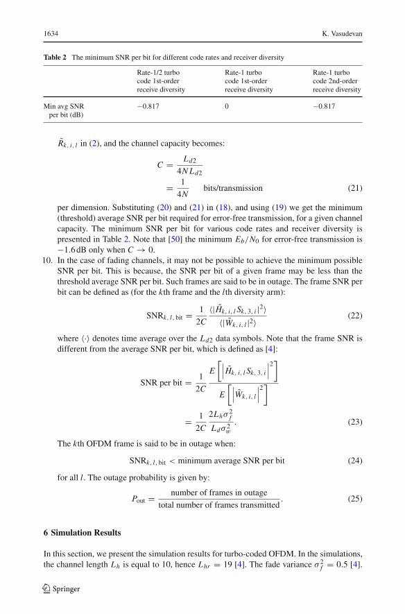
per dimension. Substituting (20) and (21) in (18), and using (19) we get the minimum(threshold) average SNR per bit required for error-free transmission, for a given channelcapacity. The minimum SNR per bit for various code rates and receiver diversity ispresented in Table 2. Note that [50] the minimum Eb/N0 for error-free transmission is−1.6dB only when C → 0.

10. In the case of fading channels, it may not be possible to achieve the minimum possibleSNR per bit. This is because, the SNR per bit of a given frame may be less than thethreshold average SNR per bit. Such frames are said to be in outage. The frame SNR perbit can be defined as (for the kth frame and the lth diversity arm):

SNRk, l, bit = 1

2C

〈|Hk, i, l Sk, 3, i |2〉〈|Wk, i, l |2〉

(22)

where 〈·〉 denotes time average over the Ld2 data symbols. Note that the frame SNR isdifferent from the average SNR per bit, which is defined as [4]:

SNR per bit = 1

2C

E

[∣∣∣Hk, i, l Sk, 3, i∣∣∣2]

E

[∣∣∣Wk, i, l

∣∣∣2]

= 1

2C

2Lhσ2f

Ldσ 2w

. (23)

The kth OFDM frame is said to be in outage when:

SNRk, l, bit < minimum average SNR per bit (24)

for all l. The outage probability is given by:

Pout = number of frames in outage

total number of frames transmitted. (25)

6 Simulation Results

In this section, we present the simulation results for turbo-coded OFDM. In the simulations,the channel length Lh is equal to 10, hence Lhr = 19 [4]. The fade variance σ 2

f = 0.5 [4].

123

Frequency Selective Rayleigh Fading Channels 1635

1.0e-03

1.0e-02

1.0e-01

1.0e+00

0 1 2 3 4 5 6 7 8

UC, data=512, PrTC, data=512, Pr

UC, data=1024, PrTC, data=1024, PrUC, data=4096, PrTC, data=4096, PrUC, data=4096, IdTC, data=4096, Id

SNR per bit (dB)

Bit

erro

r rat

e

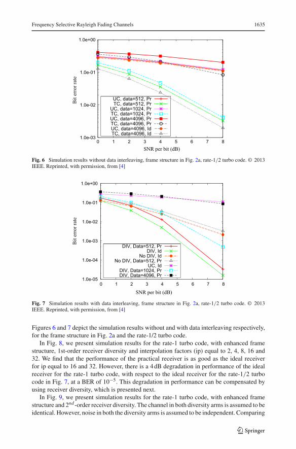
Fig. 6 Simulation results without data interleaving, frame structure in Fig. 2a, rate-1/2 turbo code. © 2013IEEE. Reprinted, with permission, from [4]

1.0e-05

1.0e-04

1.0e-03

1.0e-02

1.0e-01

1.0e+00

0 1 2 3 4 5 6 7 8

DIV, Data=512, PrDIV, Id

No DIV, IdNo DIV, Data=512, Pr

UC, IdDIV, Data=1024, PrDIV, Data=4096, Pr

SNR per bit (dB)

Bit

erro

r rat

e

Fig. 7 Simulation results with data interleaving, frame structure in Fig. 2a, rate-1/2 turbo code. © 2013IEEE. Reprinted, with permission, from [4]

Figures 6 and 7 depict the simulation results without and with data interleaving respectively,for the frame structure in Fig. 2a and the rate-1/2 turbo code.

In Fig. 8, we present simulation results for the rate-1 turbo code, with enhanced framestructure, 1st-order receiver diversity and interpolation factors (ip) equal to 2, 4, 8, 16 and32. We find that the performance of the practical receiver is as good as the ideal receiverfor ip equal to 16 and 32. However, there is a 4dB degradation in performance of the idealreceiver for the rate-1 turbo code, with respect to the ideal receiver for the rate-1/2 turbocode in Fig. 7, at a BER of 10−5. This degradation in performance can be compensated byusing receiver diversity, which is presented next.

In Fig. 9, we present simulation results for the rate-1 turbo code, with enhanced framestructure and 2nd -order receiver diversity. The channel in both diversity arms is assumed to beidentical. However, noise in both the diversity arms is assumed to be independent. Comparing

123

1636 K. Vasudevan

1.0e-05

1.0e-04

1.0e-03

1.0e-02

1.0e-01

1.0e+00

0 2 4 6 8 10 12

ip=32, Prip=16, Prip=8, Prip=4, Prip=2, Pr

Id

SNR per bit (dB)

Bit

erro

rra

te

Fig. 8 Simulation results with data interleaving, enhanced frame structure in Fig. 1a and rate-1 turbo code

1.0e-06

1.0e-05

1.0e-04

1.0e-03

1.0e-02

1.0e-01

1.0e+00

2 4 6 8 10 12 14

ip=32, Prip=16, Pr

ip=8, Prip=4, Prip=2, Pr

Id

SNR per bit (dB)

Bit

erro

r rat

e

Fig. 9 Simulation results with data interleaving, enhanced frame structure in Fig. 1a and rate-1 turbo codewith 2nd order receive diversity. Identical channel on both diversity arms

Figs. 8 and 9, we find that the ideal receiver with 2nd-order diversity is just 2dB better thanthe one with 1st-order diversity, at a BER of 10−5. Moreover, the practical receivers, withip=32 have nearly identical performance. This is to be expected, since it is well known thatdiversity advantage is obtained only when the channels are independent.

In Fig. 10, we present simulation results for the rate-1 turbo code, with enhanced framestructure and 2nd-order receiver diversity. The channel and noise in both diversity arms areassumed to be independent. Comparing Figs. 8 and 10, we find that the ideal receiver with2nd order diversity exhibits about 5dB improvement over the one with 1st order diversity, ata BER of 10−5. Moreover, the practical receiver with ip=16, 32 is just 1dB inferior to theideal receiver, at a BER of 10−5.

Finally, in Fig. 11 we present the outage probability for the rate-1 turbo code with 1stand 2nd order receive diversity. The outage probability for 1st order receive diversity, at6dB SNR per bit is 3 × 10−4. In other words, 3 out of 104 frames are in outage (no error

123

Frequency Selective Rayleigh Fading Channels 1637

1.0e-07

1.0e-06

1.0e-05

1.0e-04

1.0e-03

1.0e-02

1.0e-01

1.0e+00

3 4 5 6 7 8 9

ip=32, Prip=16, Prip=8, Prip=4, Prip=2, Pr

Id

SNR per bit (dB)

Bit

erro

r rat

e

Fig. 10 Simulation results with data interleaving, enhanced frame structure in Fig. 1a and rate-1 turbo codewith 2nd order receive diversity. Independent channel on both diversity arms

1.0e-04

1.0e-03

1.0e-02

1.0e-01

1.0e+00

-1 0 1 2 3 4 5 6

Div=1Div=2

SNR per bit (dB)

Out

age

pro

babi

lity

Fig. 11 Simulation results for outage probability with data interleaving, enhanced frame structure in Fig. 1aand rate-1 turbo code with 1st and 2nd order receive diversity. Independent channel on both diversity arms

correcting code can correct errors in such frames). Therefore, in the worst case, the numberof bit errors for the frames in outage would be 0.5 × 3 × 3,832 (assuming probability oferror is 0.5). Let us also assume that for the remaining (10,000 − 3 = 9,997) frames, allerrors are corrected, using a sufficiently powerful error correcting code. Therefore, in thebest case situation, the overall BER at 6dB SNR per bit, with 1st order diversity would be0.5 × 3 × 3,832/(10,000 × 3,832) = 1.5 × 10−4. However, from Fig. 8, even the idealcoherent receiver exhibits a BER as high as 10−2 at 6dB SNR per bit. Therefore, there islarge scope for improvement, using perhaps a more powerful error correcting code. However,it has been found from simulations that, increasing the number of trellis states does not resultin a significant improvement in the BER performance. This is probably due to the fact thatpuncturing leads to loss of information.

Similarly we observe from Fig. 11 that, with 2nd order receive diversity, the outageprobability is 10−4 at 3dB SNR per bit. This implies that 1 out of 104 frames is in outage.

123

1638 K. Vasudevan

Using similar arguments, the best case overall BER at 3dB SNR per bit would be 0.5 ×3,832/(10,000 × 3,832) = 0.5 × 10−4. From Fig. 10, the ideal coherent receiver gives aBER of 2 × 10−2, at 3dB SNR per bit, once again suggesting that there is large scope forimprovement.

7 Conclusions and Future Work

This paper deals with linear complexity coherent detectors for turbo-coded OFDM signalstransmitted over frequency selective Rayleigh fading channels. Simulation results show thatit is possible to achieve a BER of 10−5 at an SNR per bit of 8dB and throughput equal to82.84%, using a single transmit and two receive antennas.

With the rapid advances in VLSI technology, it is expected that coherent transceiverswould drive the future wireless telecommunication systems.

It may be possible to further improve the performance, using a better code.

Open Access This article is distributed under the terms of the Creative Commons Attribution License whichpermits any use, distribution, and reproduction in any medium, provided the original author(s) and the sourceare credited.

8 An Approximate and Simple Cramér–Rao Bound on the Variance of the FrequencyOffset Estimation Error

Consider the signal model in eq. (5) of [4], which is repeated here for convenience (fornotational simplicity, we drop the subscript k, assume θk = 0 and N − 1 = L p − Lh + 1):

rn = ynejωn + wn for 0 ≤ n ≤ N − 1. (26)

We assume that the channel is known, and hence yn is known at the receiver. Moreover, weconsider only the steady-state preamble part of the received signal (note that time is suitablyre-indexed, such that the first steady-state sample is considered as time zero, whereas, actuallythe first steady-state sample occurs at time Lh − 1). Define

y = [y0 . . . yN−1

]

r = [r0 . . . rN−1

]. (27)

The coherent maximum likelihood (ML) estimate of the frequency offset is obtained asfollows: choose that value of ω which maximizes the joint conditional pdf

maxω∈[−ωmax, ωmax]

p(r|y, ω

)(28)

where ωmax denotes the maximum possible frequency offset in radians. Substituting for thejoint conditional pdf in (28), we obtain

maxω

1

(2πσ 2w)N

exp

⎛⎜⎝

−∑N−1n=0

∣∣∣rn − yn e j ωn∣∣∣2

2σ 2w

⎞⎟⎠ (29)

123

Frequency Selective Rayleigh Fading Channels 1639

which simplifies to

maxω

�{N−1∑n=0

rn y∗n e

−j ωn

}. (30)

Observe that eq. (32) in [4] is the non-coherent ML frequency offset (and timing) estimator,whereas (30) is the coherent ML frequency offset estimator assuming timing is known.The root-mean-squared (RMS) frequency offset estimation error for the coherent detector isshown in Fig. 3 as “RMS coho”.

Since ML estimators are unbiased, the variance of the frequency offset estimate is lowerbounded by the Cramér–Rao bound (CRB):

E[(

ω − ω)2] ≥ 1

/E

[(∂

∂ωln p (r|y, ω)

)2]

(31)

since y is assumed to be known. It can be shown that

∂

∂ωln p (r|y, ω) = j

2σ 2w

N−1∑n=0

[n yne

jωnw∗n − n y∗

ne−jωnwn

]. (32)

Substituting (32) in (31) and assuming independent noise (the real and imaginary parts ofnoise are also assumed independent), we obtain:

E

[(∂

∂ωln p (r|y, ω)

)2]

= 1

σ 2w

N−1∑n=0

n2 |yn |2 (33)

and hence

E[(

ω − ω)2] ≥

[1

σ 2w

N−1∑n=0

n2 |yn |2]−1

(34)

when yn is known. When yn is a random variable, which is true in our case, then the righthand side of (34) needs to be further averaged over y [53,54]. In other words, we need tocompute

E

⎡⎣(

1

σ 2w

N−1∑n=0

n2 |yn |2)−1⎤

⎦ =∫

y

[1

σ 2w

N−1∑n=0

n2 |yn |2]−1

p(y) d y (35)

which is complicated. The purpose of this Appendix is to provide an alternate and a muchsimpler solution to (35), by assuming that yn is ergodic.

We claim that, for large values of N (in our case N = 504)

N−1∑n=0

n2 |yn |2 ≈N−1∑n=0

n2E[|yn |2

]

= a constant. (36)

Now

yn =Lh−1∑i=0

hi sn−i . (37)

123

1640 K. Vasudevan

Therefore

E[|yn |2

]= E

⎡⎣

Lh−1∑i=0

hi sn−i

Lh−1∑j=0

h∗j s

∗n− j

⎤⎦

=Lh−1∑i=0

Lh−1∑j=0

E[hi h

∗j

]E[sn−i s

∗n− j

](38)

where we have assumed

1. hn and sn to be independent2. sn (the preamble) varies randomly from frame to frame and is not a constant.

Hence (38) can be rewritten as:

E[|yn |2

]=

Lh−1∑i=0

Lh−1∑j=0

2σ 2f δK (i − j)σ 2

s δK ( j − i)

= 2σ 2f σ

2s Lh . (39)

where σ 2f is defined in eq. (2) of [4], σ

2s is defined in eq. (2) of [4] and δK (·) is the Kronecker

delta function. With these developments (35) becomes

E

⎡⎣(

1

σ 2w

N−1∑n=0

n2 |yn |2)−1⎤

⎦ ≈[2σ 2

f σ2s Lh

σ 2w

N−1∑n=0

n2]−1

. (40)

Therefore, theCRBon the variance of the frequency offset estimate is (assuming N−1 = M)

E[(

ω − ω)2] ≥

[2σ 2

f σ2s Lh

σ 2w

(M3

3+ M2

2+ M

6

)]−1

. (41)

The approximate CRB is depicted in Fig. 3 as “Approx CRB”.

References

1. Hanzo, L., El-Hajjar, M., & Alamri, O. (2011). Near-capacity wireless transceivers and cooperativecommunications in the MIMO Era: Evolution of standards, waveform design, and future perspectives.Proceedings of the IEEE, 99(8), 1343–1385.

2. Zhang,R., et al. (2013).Advances in base- andmobile-station aided cooperativewireless communications.IEEE Vehicular Technology Magazine, 8(1), 57–69.

3. Hanzo, L., Haas, H., Imre, S., Brien, D. O., Rupp, M., & Gyongyosi, L. (2012). Wireless myths, real-ities, and futures: From 3G/4G to optical and quantum wireless. Proceedings of the IEEE, 100(SpecialCentennial issue), 1853–1888.

4. Vasudevan, K. (2013). Coherent detection of turbo coded OFDM signals transmitted through frequencyselective rayleigh fading channels. In Proceedings of the IEEE ISPCC. Shimla, India, Sept. 2013.

5. Samal, U. C., & Vasudevan, K. (2013). Bandwidth efficient turbo coded OFDM systems. In Proceedingsof the IEEE ITST (pp. 490–495), Tampere, Finland, Nov. 2013.

6. Bingham, J. A. C. (1990). Multicarrier modulation for data transmission: An idea whose time has come.IEEE Communications Magazine, 28(5), 5–14.

7. Vasudevan, K. (2010). Digital communications and signal processing, (CDROM included), 2nd edn.(India), Hyderabad: Universities Press. www.universitiespress.com.

8. Hanzo, L., & Keller, T. (2006). OFDM and MC-CDMA: A primer. New York: Wiley.9. Schmidl, T. M., & Cox, D. C. (1997). Robust frequency and timing synchronization for OFDM. IEEE

Transactions on Communications, 45(12), 1613–1621.

123

Frequency Selective Rayleigh Fading Channels 1641

10. van de Beek, J.-J., Sandell,M., Isaksson,M., &Börjesson, P. O. (1995). Low-complex frame synchroniza-tion in OFDM systems. In Proceedings of the 4th IEEE international conference on universal personalcommunications, Nov. 1995 (pp. 982–986). Tokyo, Japan.

11. Landström, D., Wilson, S. K., van de Beek, J.-J., Ödling, P., & Börjesson, P. O. (2002). Symbol timeoffset estimation in coherent OFDM systems. IEEE Transactions on Communications, 50(4), 545–549.

12. Park, B., Cheon, H., Kang, C., & Hong, D. (2003). A novel timing estimation method for OFDM systems.IEEE Communications Letters, 7(5), 239–241.

13. Ren, G., Chang, Y., Zhang, H., & Zhang, H. (2005). Synchronization method based on a new constantenvelope preamble for OFDM systems. IEEE Transactions on Broadcasting, 51(1), 139–143.

14. Kang, Y., Kim, S., Ahn, D., &Lee, H. (2008). Timing estimation for OFDMsystems by using a correlationsequence of preamble. IEEE Transactions on Consumer Electronics, 54(4), 1600–1608.

15. Baum, K. L. (1998). A synchronous coherent OFDM air interface concept for high data rate cellularsystems. In Proceedings of the IEEE VTS 48th vehicular technology conference, May 1998, pp. 2222–2226.

16. Julia Fernández-GetinoGarcia,M., Edfors, O., & Páez-Borrallo, J.M. (2001). Frequency offset correctionfor coherent OFDM in wireless systems. IEEE Transactions on Consumer Electronics, 47(1), 187–193.

17. Bradaric, I., & Petropulu, A. P. (2003). Blind estimation of the carrier frequency offset in OFDM systems.In 4th IEEE workshop on signal processing advances in wireless communications, June 2003, (pp. 590–594).

18. Kuo, C., & Chang, J.-F. (2005). Generalized frequency offset estimation in ofdm systems using periodictraining symbol. In Proceedings of the IEEE international conference on communication, May 2005, pp.715–719.

19. Lin, J.-S., & Chen, C.-C. (2005). Hybrid maximum likelihood frequency offset estimation in coherentOFDM systems. IEE Proceedings - Communications, 152(5), 587–592.

20. Ahn, S., Lee, C., Kim, S., Yoon, S. & Kim, S. Y. (2007). A novel scheme for frequency offset estimationin OFDM systems. In 9th international conference on advanced communication technology, Feb. 2007,pp. 1632–1635.

21. Henkel, M., & Schroer, W. (2007). Pilot based synchronization strategy for a coherent OFDM receiver.In IEEE wireless communications and networking conference (WCNC), March 2007, pp. 1984–1988.

22. Tufvesson, F., Edfors, O., & Faulkner, M. (1999). Time and frequency synchronization for OFDM usingPN-sequence preambles. In Proceedings of the IEEE VTS 50th vehicular technology conference, Sept.1999, pp. 2203–2207.

23. Minn, H., Bhargava, V. K., & Letaief, K. B. (2003). A robust timing and frequency synchronization forOFDM systems. IEEE Transactions on Wireless Communication, 2(4), 822–839.

24. Zhang, Z., Long, K., Zhao, M., & Liu, Y. (2005). Joint frame synchronization and frequency offsetestimation in OFDM systems. IEEE Transactions on Broadcasting, 51(3), 389–394.

25. Abdzadeh-Ziabari, H., & Shayesteh, M. G. (2011). Robust timing and frequency synchronization forOFDM systems. IEEE Transactions on Vehicular Technology, 60(8), 3646–3656.

26. Mattera, D., & Tanda, M. (2013). Blind symbol timing and CFO estimation for OFDM/OQAM systems.IEEE Transactions on Wireless Communications, 12(1), 268–277.

27. López-Salcedo, J. A., Gutiérrez, E., Seco-Granados, G., & Swindlehurst, A. L. (2013). Unified frameworkfor the synchronization of flexible multicarrier communication signals. IEEE Transactions on SignalProcessing, 61(4), 828–842.

28. Frenger, P. K., & Svensson, N. A. B. (1999). Decision-directed coherent detection in multicarrier systemson Rayleigh fading channels. IEEE Transactions on Vehicular Technology, 48(2), 490–498.

29. Merli, F. Z., &Vitetta, G.M. (2008). A factor graph approach to the iterative detection of OFDM signals inthe presence of carrier frequency offset and phase noise. IEEE Transactions onWireless Communications,7(3), 868–877.

30. wei Wang, H., Lin, D. W., & Sang, T.-H. (2012). OFDM signal detection in doubly selective channelswith blockwise whitening of residual intercarrier interference and noise. IEEE Journal on Selected Areasin Communications, 30(4), 684–694.

31. Chen, C.-Y., Lan, Y.-Y., & Chiueh, T.-D. (2013). Turbo receiver with ICI-aware dual-list detection formobile MIMO-OFDM systems. IEEE Transactions on Wireless Communications, 12(1), 100–111.

32. van deBeek, J.-J., Edfors, O., Sandell,M.,Wilson, S. K., &Börjesson, P. O. (1995). On channel estimationin OFDM systems. In Proceedings of the IEEE VTS 45th vehicular technology conference, July 1995, pp.815–819.

33. Edfors, O., Sandell, M., van de Beek, J.-J., Wilson, S. K., & Börjesson, P. O. (1998). OFDM channelestimation by singular value decomposition. IEEE Transactions on Communications, 46(7), 931–939.

34. Coleri, S., Ergen, M., Puri, A., & Bahai, A. (2002). Channel estimation techniques based on pilot arrange-ment in OFDM systems. IEEE Transactions on Broadcasting, 48(3), 223–229.

123

1642 K. Vasudevan

35. Ribeiro, C., & Gameiro, A. (2008). An OFDM symbol design for reduced complexity MMSE channelestimation. Journal of Communications, 3(4), 26–33.

36. Kinjo, S. (2008). An MMSE channel estimation algorithm based on the conjugate gradient methodfor OFDM systems. In The 23rd international technical conference on circuits/systems, computers andcommunications (ITC-CSCC), July 2008, pp. 969–972.

37. Jiang,M., Akhtman, J., &Hanzo, L. (2007). Iterative joint channel estimation andmulti-user detection formultiple-antenna aided OFDM systems. IEEE Transactions on Wireless Communications, 6(8), 2904–2914.

38. Fischer, R. F. H., Lampe, L. H.-J., &Müller-Weinfurtner, S. H. (2001). Codedmodulation for noncoherentreception with application to OFDM. IEEE Transactions on Vehicular Technology, 50(4), 910–919.

39. Marey, M., Samir, M., & Dobre, O. A. (2012). EM-based joint channel estimation and IQ imbalances forOFDM systems. IEEE Transactions on Broadcasting, 58(1), 106–113.

40. Kamalian, M., Tadaion, A. A., &Derakhtian, M. (2012). Invariant detection of orthogonal frequency divi-sion multiplexing signals with unknown parameters for cognitive radio applications. IET Signal Process-ing, 6(3), 205–212.

41. Turunen, V., Kosunen, M., Vä ä rä kangas, M., & Ryynä nen, J. (2012). Correlation-based detection ofOFDM signals in the angular domain. IEEE Transactions on Vehicular Technology, 61(3), 951–958.

42. Tan, P.,&Beaulieu,N.C. (2006).A comparison ofDCT-basedOFDMandDFT-basedOFDMin frequencyoffset and fading channels. IEEE Transactions on Communications, 54(11), 2113–2125.

43. Yu, C., Sung, C.-H., Kuo, C.-H., Yen, M.-H., & Chen, S.-J. (2012). Design and implementation of alow-power OFDM receiver for wireless communications. IEEE Transactions on Consumer Electronics,58(3), 739–745.

44. Sari, H., Karam, G., & Jeanclaude, I. (1995). Transmission techniques for digital terrestrial TV broad-casting. IEEE Communications Magazine, 33(2), 100–109.

45. Reimers, U. (1998). Digital video broadcasting. IEEE Communications Magazine, 36(6), 104–110.46. Takahashi, H. (2009). Coherent OFDM transmission with high spectral efficiency. In 35th European

conference on optical communication, Sept. 2009, (pp. 1–4).47. Vasudevan, K. (2008). Synchronization of bursty offset QPSK signals in the presence of frequency offset

and noise. In Proceedings of the IEEE TENCON, Hyderabad, India, Nov. 2008.48. Vasudevan, K. (2012). Iterative detection of turbo coded offset QPSK in the presence of frequency and

clock offsets and AWGN. Signal, Image and Video Processing, 6(4), 557–567.49. Adakane, D. V., & Vasudevan, K. (2013). An efficient pilot pattern design for channel estimation in

OFDM systems. In Proceedings of the IEEE ISPCC, Shimla, India, Sept. 2013.50. Proakis, J. G., & Salehi, M. (2005). Fundamentals of communication systems. Pearson Education Inc.51. Haykin, S. (2001). Communication systems (4th ed.). New York: Wiley Eastern.52. Proakis, J. G. (1995). Digital communications (3rd ed.). New York: McGraw Hill.53. Morelli,M.,&Mengali,U. (2000).Carrier-frequency estimation for transmissions over selective channels.

IEEE Transactions on Communications, 48(9), 1580–1589.54. Li, Y., Minn, H., & Zeng, J. (2010). An average Cramer–Rao bound for frequency offset estimation in

frequency-selective fading channels. IEEE Transactions on Wireless Communications, 9(3), 871–875.

K. Vasudevan completed his Bachelor of Technology (Honours) fromthe department of Electronics and Electrical Communication Engineer-ing, IIT Kharagpur, India, in the year 1991, and his M.S. and Ph.D.from the department of Electrical Engineering, IIT Madras, in the years1996 and 2000 respectively. During 1991–1992, he was employed withIndian Telephone Industries Ltd, Bangalore, India. He was a Post Doc-toral Fellow at the Mobile Communications Lab, EPFL, Switzerland,between Dec. 1999 and Dec. 2000, and an engineer at Texas Instru-ments, Bangalore, between Jan 2001 and June 2001. Since July 2001,he has been a faculty at the Electrical department at IIT Kanpur, wherehe is now an Associate Professor. His interests lie in the area of com-munications and signal processing.

123