Embed Size (px)
Citation preview

Cognitive Vision Model Gauging Interest in
Advertising Hoardings
Saad Choudri
MSc Cognitive Systems Session 2005/2006 The candidate confirms that the work submitted is his own and the appropriate credit has been given where reference has been made to the work of others. I understand that failure to attribute material which is obtained from another source may be considered as plagiarism.
(Signature of student) ___________________________________

For the late Vice Admiral HMS Choudri (H.Pk ; MBE), my grandfather, friend and mentor.
i

Acknowledgments At the outset, I would like to acknowledge the support of my parents Rishad and Samar Choudri
who encouraged and sponsored my MSc Cognitive Systems. My other family members and friends
who supported me considerably include Sana Lutfullah, Rayika, Zayd and Khizar Diwan to whom I
am thankful.
Prof. David Hogg (Supervisor) and Dr. Andy Bulpit (Assessor), with their unmatched experience in
Computer Vision and guidance, fueled the “from idea to project” concept to help me refine the
conception of this project.
Prof. David Hogg supported this project from the very start and most of all encouraged a self-driven
approach which in itself had immense advantages including novelty. Dr. Hannah Dee (stand-in
Supervisor) played a vital role in his absence to steer the report toward its current state and make me
think “Japanese garden” vs. “English garden”.
I am very grateful to Eric Atwell for giving me an edge for the road ahead and to Katja Markert,
Prof. Tony Cohn, Prof. Ken Brodlie, Martyn Clark and Tony Jenkins for various roles they played.
I would also like to thank all members of [email protected] including Savio Pirondini,
Graham Hardman and Pritpal Rehal for none other than their support.
Special thanks to Simon Baker and Ralph Gross at Carnegie Mellon University for making available
the Pose Illumination and Expression (PIE) database of 41368 images.
Thanks to Lee Kitching and Khurram Ahmed for participating in a few evaluation videos. Mention
must also be made of Arnold, the silverfish in my room who, if he could, would gladly have eaten
this report.
Last but not least, I would like to thank administration members of the School of Computing,
especially Mrs. Irene Rudling, Yasmeen, Judy and Teresa for, among other assistance, helping me
locate Prof. Hogg for my million plus questions.
ii

Abstract
In order to gauge pedestrian interest in advertising hoardings, a gaze or head pose estimation system
is required. Proposed here, is a novel “spirit-level” approach to head pose estimation where heads
may be as small as 20 pixels high and lack detail. This adds to the few existing models that deal
with such head sizes. The heads are found using a Viola-Jones model for face detection. A binary
feature vector drawn horizontally from approximately the centre of the eyes and tip of the nose
consists of skin pixels as a bubble against non-skin pixels. The feature vector is classified by a
support vector machine classifier previously trained and containing a number of support vectors for
three generalised head poses; left, right and centre. Designed specifically to gauge interest in
advertisement hoardings, the model is complemented with a regional interest gauge to measure
interest in specific objects. A hoarding is divided into nine regions and 5 discretised face kernel
templates are used to classify the region of interest, in a combination of two or more classifications.
The “spirit-level” system performs at par with other existing systems at 89% accuracy.
iii

Table of Contents
Chapter 1: Introduction........................................................................................................................ 1
1.1 Motivation ................................................................................................................................. 1
1.2 Project Overview....................................................................................................................... 1
1.2.1 Aim and Objective ............................................................................................................. 1
1.2.3 Requirements ..................................................................................................................... 2
1.2.4 Enhancements .................................................................................................................... 2
1.2.5 Deliverables ....................................................................................................................... 2
1.3 Scope ......................................................................................................................................... 2
1.4 Methodology ............................................................................................................................. 4
1.4.1 Outline Description and Specification ............................................................................... 4
1.4.1.1 Research Methods....................................................................................................... 5
1.4.1.2 Schedule...................................................................................................................... 5
1.4.2 Development and Validation.............................................................................................. 5
Chapter 2: Background and Previous Work ........................................................................................ 7
2.1 Literature Review: Background ................................................................................................ 7
2.2 Literature Review: Possible Solutions....................................................................................... 8
2.2.1 Determining Direction of Gaze at Close Range................................................................. 8
2.2.2 Determining Direction of Gaze at a Distance .................................................................... 9
2.2.3 Detecting the Face and Eyes ............................................................................................ 11
2.3 Literature Review: Machine Learning..................................................................................... 14
2.3.1 Regression Trees vs. Classification Trees........................................................................ 15
2.3.2 Support Vector Machines vs. Neural Networks............................................................... 15
2.3.3 Partition-Based vs. Hierarchical Clustering ..................................................................... 17
2.3.4 Mahalanobis Distance vs. Euclidean Distance................................................................. 17
Chapter 3: Model and Experiment Design......................................................................................... 19
3.1 Development Environment...................................................................................................... 19
3.2 Dataset ..................................................................................................................................... 19
3.3 Component Analysis and Testing............................................................................................ 21
3.4 Testing and Training Data ....................................................................................................... 22
Chapter 4: Experimental Feature Based Model ................................................................................. 23
4.1 Plan and Architecture .............................................................................................................. 23
4.1.1 Integrating MPT and Feature Extraction.......................................................................... 24
4.1.2 Classification.................................................................................................................... 26
4.2 Evaluation................................................................................................................................ 27
iv

Chapter 5: Spirit-Level and Face Kernels.......................................................................................... 31
5.1 Plan and Architecture .............................................................................................................. 31
5.1.1 Initial Version .................................................................................................................. 33
5.1.2 Image Segmentation Explored ......................................................................................... 38
5.2 Spirit-Level Approach ............................................................................................................. 43
5.3 Cross-Referencing Objects With Pose Using Face Kernels .................................................... 44
5.4 Evaluation of the Final Model including Spirit-Level vs. 13 Features.................................... 46
5.5 Final Model Combined............................................................................................................ 49
Chapter 6: Evaluation Against Ground Truth.................................................................................... 51
6.1 The Set Up............................................................................................................................... 51
6.2 MPT’s Suitability .................................................................................................................... 52
6.3 Robustness............................................................................................................................... 53
6.4 DoG Estimation Ability........................................................................................................... 54
6.5 Evaluation Summary ............................................................................................................... 58
Chapter 7: Future Work ..................................................................................................................... 59
Chapter 8: Conclusion ....................................................................................................................... 60
References.......................................................................................................................................... 61
Appendix A: Reflection ..................................................................................................................... 65
Appendix B: Objectives and Deliverables Form ............................................................................... 66
Appendix C: Marking Scheme and Header Sheet ............................................................................. 67
Appendix D: Gantt Chart and Project Management .......................................................................... 70
Appendix E: CD ................................................................................................................................ 71
Appendix F: Dataset .......................................................................................................................... 72
Appendix G: 13 Feature Analysis Samples ....................................................................................... 74
Appendix H: Image Segmentation Samples ...................................................................................... 76
Appendix I: Ground Truth Evaluation Form ..................................................................................... 83
v

Chapter 1: Introduction Provided here is the basis and scope for the project to set the scene for the rest of the report.
1.1 Motivation
During 2005, an estimated £196m [1] was invested in outdoor advertising in the United Kingdom.
Competing firms in consumer markets employ advertising companies to get their messages across.
Whether advertisement hoardings, “in-game advertising” or internet advertising, success is often
gauged in sales reports. Amongst the mediums mentioned, hoardings are widely used. It is easy to
make a pretty picture and attach a message to it but to actually determine what people are looking at,
what market demographics are looking, what expressions the observers have and how long they
gaze for is data that is sought after by all. Gaze estimation data is essential in that it allows
advertisers to see what attracts attention most, the model in the image, the product message, the
company logo, and possibly even the location of the hoarding. Viable solutions can be adapted from
within the field of Computer Vision (CV). Benefits will include allowing firms to test their
approaches to advertising on a smaller scale, before making large commitments to clients. But while
gaze estimation has been researched extensively for close-range subjects, limited attention has been
given to outdoor situations.
1.2 Project Overview
1.2.1 Aim and Objective
This projects aim was to design, implement and evaluate a CV model to gauge if pedestrians are
showing interest in advertisement hoardings. This was to be done by estimating their viewing
direction and duration. Hence, it primarily set out to answer the question; “is someone in the video
looking towards the hoarding or not, and if so then for how long”. The approach was to combine
state-of-the-art face and eye detection techniques with self-implemented algorithms. Though this
was only the beginning of a solution for the motivating requirements, it was a challenging task to
undertake and provides a novel platform for future work.
The educational objective here was to get “hands-on” experience in implementing CV techniques
and Machine Learning (ML) for a “real-world” problem. This is always the ideal way to learn and is
the purpose of most academic projects. The acquisition of this experience and knowledge gained
along the way was intended to be good enough to tackle several areas where CV could be used to
solve problems. This endeavour was also an exercise in project management skills- the ability to
schedule, organise, research and troubleshoot effectively.
1

1.2.3 Requirements
The minimum requirements provided a basis to expand on. They were:
1. Integrate off-the-shelf face and eye detection software.
2. Estimate viewing direction using a face and eye detection package augmented with novel
algorithms and, or, approaches through literature research.
3. Devise a measure of interest from viewing angle and duration of viewing.
4. Evaluate the system documented in a report.
Since this project was an idea, i.e., without an industry representative, this was the “requirements
elicitation phase” in the “requirements engineering process” as described in [2] and [3].
1.2.4 Enhancements
There were a number of potential optional enhancements that could have been incorporated. These
included:
1. Incorporation of facial expression or gesture recognition.
2. Cross-reference of gaze to objects in the display to gauge level of interest in an object.
1.2.5 Deliverables
These deliverables were discussed and agreed:
1. Project report with an evaluation from ground truth, i.e. video footage from a hoarding.
2. The video used in the evaluation, could be from a ground level hoarding etc.
3. Software, i.e. source code.
1.3 Scope
An elaboration on the minimum requirements and what the project was meant to do is described
here. This report’s style assumes the reader is familiar with CV. Integrating off-the-shelf face and
eye detection software involved studying to see if the suggested (in formal discussions) Machine
Perception Toolbox (MPT) would be ideal to use. Similar steps to the Component Based Software
Engineering (CBSE) methodology described in [2] and [3] were taken at the start to see if the
Machine Perception Toolbox (MPT) [29] component would be ideal with careful attention to ensure
that no requirements adjustment [2] be required. The decision was made on the basis of; 1) if there
were other papers describing its use; 2) if it performed well enough for the algorithm under
development to be evaluated. A detailed study of all existing face detection packages was outside
the scope of this project and non-functional aspects such as memory usage were not deciding
2

factors. Though the concept of emergence [3, 5] within such a component based system existed,
such details would have disrupted the schedule.
Figure 1.1 (from left to right) Right, centre and left poses (laterally inverted). Source [4]
Estimating viewing direction, requirement two, was to be dependent on the training images
available and the fact that hoardings in general vary in size, shape, and location. Thus it was decided
that three generalised limits as shown in Figure 1.1 would be the basic left, centre and right
representatives for the development of the project, and if the model correctly classified these above
a Zero R baseline, it would be a decent proposal to the problem. It is important to note that head
pose estimation is mainly for pedestrians. It does not apply to anyone in a motorised vehicle where
the face is often obscured or unclear. Therefore it is more useful in countries where target
consumers travel generally on foot, such as most of Europe and the United States rather than
countries like Pakistan, where consumers are normally hidden in automobiles. It was also not
necessarily required to work on faces with accessories such as hats or veils, but if it did this was an
advantage. Spectacles and sunglasses were considered a challenge and were included in what the
system should have worked with. As for the machine learning methods chosen, a brief justification
is provided rather than an extensive survey. This project was meant to explore a non-model based
approach. Therefore techniques such as principal component analysis (PCA) [9] were left out.
Requirement 3, devising an interest measure, should be interpreted in its basic sense as taking the
gaze estimation model from requirement 2 and using it to count in total the seconds or “duration”
that the billboard was viewed for. This does not take into account how many people viewed it but
simply a “viewed or not viewed” count, per face, per frame. This is not required of all the iterations
and prototypes that were developed. Instead only the prototype which outperforms the rest,
according to an evaluation criteria discussed later, will be further tuned to measure this duration in
either a text form or an image annotation.
The further enhancements include two possibilities. The first is facial gesture or facial expression
recognition, and the second involves cross-referencing objects in the hoarding with the estimated
head pose. The latter was not supposed to say precisely what object was being viewed but instead a
regional interest estimate would have sufficed. This was because object recognition or any similar
approaches were beyond the scope of this project. Therefore a count will be incremented for each
region of the hoarding as it is viewed.
3

The deliverables included a report, software and evaluation video. Among these points it should be
clarified that a hoarding and billboard can be at any level and assumed to be of a size that is
normally larger than A1. Both refer mainly to a large outdoor signage or advertisement [6, 7].
Therefore the evaluation video was not specific to any hoarding. In fact, since putting a camera in
front of a billboard and not concealing it has the affect of people looking directly at the camera;
recording may be done from a simulated location. The software is in the form of a prototype source
code and not a user interfaced application as specified.
1.4 Methodology
As with most projects not involving third-party stakeholders, especially academic research oriented
types, conventional methodologies such as “the waterfall model” cannot be applied as they do not
usually require signoffs. In fact almost all projects that are not critical systems generally follow an
adapted or modified selected methodology [3]. Though publications demonstrate inconsistency in
opinion to what “prototyping” actually is [8], this methodology with its branch of “evolutionary
prototyping” is best suited to this project. Figure 1.2 best describes the overall methodology used.
Figure 1.2 Evolutionary development illustration. Source [2]
1.4.1 Outline Description and Specification
In an industrial project "outline description" and "specification" come from external requirements.
Here they emerged from the minimum requirements. Often during this phase, coined in [3] as
"requirements engineering", a risk analysis, feasibility study and cost benefit analysis are conducted.
This was avoided due to the projects nature. Instead, the schedule described in Section 1.4.1.2 was
hoped to take into account risks such as "feature-creep" [3]. Considering the fact that this
experimental project had an iterative method of development, an industry representative was not
interviewed. This is because it was feared that this would have lead to taking an overly expansive
approach with too many requirements (for example, gauging what a person is thinking) which could
have lead to failure [2, 3, 8]. In terms of “requirements analysis”, Chapter 2 presents an in-depth
problem and solution review that is a key step in this software process.
4

1.4.1.1 Research Methods
This project was centred on academia and thus it was essential to study relevant available literature
as opposed to implemented systems since the latter would have been difficult to access and appeared
not to exist. Several research papers are available on gaze and pose estimation, and face and gesture
recognition, and these were the primary source for literature research and background reading. Also,
the research was prototype specific. For example, the first prototype was based on using features
such as the eyes and the face to estimate viewing direction. For this, papers related to feature usage
were read and a few alternative techniques were looked at until a suited solution and final system
was achieved. However, the research was only a means to gain background knowledge into the
problem. The main drive behind this project was to experiment with state-of-the-art techniques
learnt during the academic year in conjunction with an “out of the box” fresh approach. This was
necessary since the project is entirely experimental and thus far appears not to have been
implemented before. To research into the problem, papers on billboard surveys, advertising
productivity and survey techniques were reviewed.
1.4.1.2 Schedule
The Gantt chart is shown in Appendix D. The project made considerable head-way within the first
few months. The plan was devised with larger milestones as past experience showed that it was not
possible to predict exactly how long smaller tasks took. For example, it took longer to determine
how best to segment a face from the background, in a non-model based way without a spleen curve
fitting algorithm, than it did to code the entire final system. This was unanticipated at the start of the
project.
1.4.2 Development and Validation
Two main prototypes were developed each with several different versions. Figure 1.3 shows 5
stages that outline this report. The first stage deals with experimentations and finding the best
combination of face and eye detection which is found throughout the report. Stage 2 shows the first
prototype which works with 13 features and caters to the minimum requirements. This is described
in Chapter 4. It is evaluated using datasets collected and described in Chapter 3. The evaluation
criterion is mainly true negatives and true positives also referred to as truth, accuracy and precision
in this report. However as explained later, algorithm bias and other factors are also taken into
account for comparison purposes. Stage 3 shows two systems. The “spirit-level” prototype,
described in Chapter 5 (part of the final model) evolved after the feature based approach described
in Chapter 4. It moves beyond the minimum requirements by dividing “not looking” into “left or
right”. It also performs far better as shown in Chapter 5’s evaluation. The further enhancement of
cross referencing objects in the billboard with head pose was also successfully developed, evaluated
and combined with the final system or model described in Chapter 5.
5

Chapter 6 puts the final model described in Chapter 5 to a “ground truth” test. Several frames of
processed video were captured at 2 second intervals over the duration of the evaluation videos shot
at various locations. These were manually evaluated and several confusion matrices were made. All
aspects were tested. The basis of testing only the final model on outdoor footage was primarily that
most texts [2, 3 & 8] agree that a prototype should be executable and the intermediate versions need
not be fully functional but should be at a simulated level. Therefore, each prototype version was
evaluated in a controlled environment as mentioned. Only the final selection was developed further
and evaluated in Chapter 6. To ensure all deadlines were met it was not possible to evaluate every
frame after it was processed which is another reason why 2 second intervals were chosen.
MPT
Face & Eyes
DoG
2
L R S
?
1
Looking?
YesNo
Experimentation with face and eye detection Chapters 3 to 6
Meeting minimum requirements with a feature
based approach Chapter 4
A novel “spirit-level” approach that addresses the minimum requirements adds features and performs better
than that in Chapter 4. Evaluated and chosen for
final system Chapter 5
3
A regional detector for cross referencing objects in
hoardings with head pose. This is added to the final
system Chapter 5
evaluated
evaluated
GROUND TRUTH EVALUATION OF FINAL
SYSTEM Chapter 6
4
5 Figure 1.3 Outline of main prototypes and report structure.
The report combines various stages of the development into similar sections for the sake of brevity
and flow. For example, the dataset selection in Chapter 3 was done over many days. First, several
photographs were taken of a subject to test the face detection component and after that a test and
training set was selected. In this report, it has all been put into one section. This can be found in
other areas as well to keep within the reports page limit. Section 5.5 describes the final model.
Appendix E contains the remaining deliverables other than the report and evaluation.
6

Chapter 2: Background and Previous Work A detailed problem analysis and extensive review into state-of-the-art CV techniques follows.
2.1 Literature Review: Background
Advertising expenditure within the U.K in 2005 stood at £ 3,027m with an increase of 4.4% forecast
for 2006. 6.5% of this was spent on outdoor advertisements (hoardings or billboards) [1]. Despite
the adspend, research on advertisings productivity is limited and fragmentary [10]. Long standing
regulatory debates also exist, but only a limited number of academic studies explore why firms use
the medium. Users claim that billboards have unique advantages not offered by other media and are
afraid that their companies will lose up to 20% sales if billboards were banned [11]. Outdoor
advertising has increased in popularity owing to its creative treatment which aims to provide new
ways of using this traditional medium [12]. However, a study in [13] reveals that treatment such as
“smart-boards” produced the lowest level of recall.
From another perspective, Advertising Standards Authority (ASA) prepares compliance reports by
assessing billboards and administers the British Codes of Advertising and Sales Promotion by
visiting boards and often adhering to complaints. Between 1st January 2002 and 30th June 2002
1577 outdoor advertisements were assessed among which a few were in breach of codes and had to
be dealt with. If a gaze estimation system was present with facial gesture recognition, inappropriate
advertisements could be identified earlier [14].
A non-CV based application that attempted to blur the boundaries between web-browsing and art-
making was called Jumboscope [15] based on Kerne’s “Collage Machine” described in [16]. The
project interactively, by detecting interest through motion sensors and a touch screen display
interaction changed collages on a large touch screen display, rating the most popular collages. The
CV technique, eye-tracking, has been used in advertising to gauge interest in internet advertisements
and improve web-designing. In fact it has become a necessity giving designers insight into the
effectiveness of their websites [17]. The most relevant use of eye-tracking is described in [18] where
research was conducted to see if adolescents attend to warnings in cigarette advertisements. The test
involved 326 adolescents who viewed several cigarette advertisements with mandated and non-
mandated health warnings. It was followed by a recall test hoping to link cognitive processes to eye
ball movement. It showed that new non-mandated warnings were most effective.
7

As is evident, there does not appear to be a system in place using state-of-the-art CV techniques for
outdoor advertisements, and if there was one it would be extremely useful. The next section presents
a detailed survey of solutions that were considered to solve this problem.
2.2 Literature Review: Possible Solutions
In order to develop a system to gauge pedestrian interest in advertisement hoardings the key was to
understand how to determine gaze so as to answer the question; “are they looking at the hoarding?”
There are several other applications requiring a good estimator of the direction of gaze and therefore
research was carried out for each area. The most prominent of these areas found in research papers
was that of human computer interfaces (HCI) and surveillance. For example, the handicapped can
use gaze to control a mouse cursor in cases where they may only be able to move their faces or
eyeballs [19]. Surveillance videos can be processed and queries in investigations, such as, if a
person was being followed, can also be answered [25]. Various approaches have been used but most
combine head pose estimation with eye location estimations and, or, body pose or sometimes
probabilistic local descriptions to find facial features like the skin.
2.2.1 Determining Direction of Gaze at Close Range
The most common and basic way to go about estimating direction of gaze (DoG) is to find the eyes
and the face associated with the eyes in an image. From this certain characteristics are extracted that
are then used. Head pose estimation and DoG in such systems depends completely on the ability of
the system to track certain facial features reliably but feature tracking itself is error-prone unless
verification and forward estimation of higher level information is done [19]. To estimate DoG in
video streams sometimes velocity and direction of movement is used in symbiosis. In some cases
just the face and direction of motion are used because problems with locating features in small poor
quality images where the face may be 20 pixels high is difficult, and eyes, for example, cannot be
found.
Gee and Cipolla’s work in [20] is heavily based on facial features and uses 3D geometric
relationships between these features. It has been applied to paintings to determine where the subject
is looking. They look at points such as nose tip and base, define a facial plane with the far corners of
the eyes and mouth and with various ratios move to two main methods, one that uses 3-D
information provided by the position of the nose tip and the image, and the other which exploits a
planar skew-symmetry. [20] While this is an excellent method for accurate gaze estimation in large
paintings it cannot be applied to images of low quality where it becomes extremely difficult to track
certain features accurately to build upon. However, their use of ratios for eye planes and other
parts of the face is built upon and abstractions can be found throughout the project.
8

As mentioned, significant work has been carried out for HCI to estimate DoG. In [21] Morimoto et
al. base their technique on the theory of spherical optical surfaces and using the Gullstrand model of
the eye to estimate the positions of the centres of the cornea and pupil in 3D. They propose a method
for computing the 3D position of an eye and its gaze direction from a single camera with two near
infra-red light sources. This approach allows for free face motion and does not require calibration
with the user before each user session [21]. Zelinsky and Heinzmann in [19] also propose a similar
method which reconstructs the eye in 3-D to account for loss of detail through illumination and
distance variation. Besides their dependency on the subject’s nearness, these two systems relied on a
“world” based coordinate system. This decision was based on Brooks’ [48] views against a “sense-
model-plan-act methodology” [48]. Results of a picture based system were far better than the
“world” based coordinate system since it avoided the “cumbersome, complex, and slow complete
world modelling approach” [48].
Other techniques include oculography, limbus, pupil and eyelid tracking, a contact lens method,
corneal and pupil reflection relationships, Purkinje image tracking, artificial neural networks,
morphable models and geometry [22]. Wang et al., in [22], propose their “one circle” algorithm for
estimating DoG combining projective geometry and anthropometric properties of the eyeball. Their
method differs from others in that they treat the image of the iris contour correctly as an ellipse,
accuracy is improved since their method only needs the image of one eye and thus greater zooming
can be done with certain mechanisms in place to avoid losing the eye while tracking it. They rely
heavily on estimating the ellipse of the iris contour and the edges of the iris. Their results were
found to be better than other non-intrusive approaches such as one proposed by Zelinsky and
Heinzmann in [19] [22].
As far as tracking is concerned, especially that of the face’s movement and flow, edge detection can
be used and combined with other estimators as has been done in [23] to understand the importance
of motion information in human-robot attention. However none of these approaches can
successfully be employed in the task at hand as they significantly rely on near proximity. Also, it
will not be enough to implement an eye ball rotation tracking system. Even though they may
produce accurate gaze estimates for a subject looking within the narrow field of view allowed by the
eye movements alone, they cannot cope with larger gaze shifts which involve a movement of the
face [20].
2.2.2 Determining Direction of Gaze at a Distance
In [24] Voit and Nickel propose a “smart room” based neural network approach to face pose
estimation and horizontal face rotation. Their motivation was to move beyond the subject sitting in
one position but is still confined to a “smart room” fitted with 4 cameras at each corner. It appears
that it can easily be extended to a market place or some outside area to suit the project at hand. A
9

good reason for this is that it does not require images to have clearly visible features. This is
beneficial because most head pose estimation techniques do and thus are not suited to distances and
the outside world. However what can be problematic is a crowd of people. The system will have to
track faces that are common to the cameras for accuracy.
Other approaches that tackle detailed-feature based problems include that of Efros who showed how
to distinguish between human activities including walking and running. Efros’ system compared the
gross properties of motion using a descriptor derived from frame-to frame optic flow and performed
an exhaustive search over extensive representative data. Although the aim was not to estimate face
pose it showed how the use of a system descriptor invariant to lighting and clothing can be useful
[25]. There are many examples where solely trajectory information is used for surveillance purposes
including that in MITs AI lab to monitor urban sites [25]. At the University of Leeds, Prof. David
Hogg and Dr. Hannah Dee use a Markov chain with penalties associated with state transitions. It
returns a score for observed trajectories which essentially encodes how directly a person made his or
her way toward predefined scene exits [25]. Such techniques can be used to identify the direction of
motion combined with other information which has been done in the work of Robertson et al. in
[25], a remarkable and major shift from the feature tracking approaches. It combines head pose and
trajectory information using Bayes rule to obtain a joint distribution [25].
This remarkable approach [25], which may be considered as an “explicit” technique, discussed later,
for estimating DoG, caters to situations where the persons face is typically 20 pixels high. It uses a
feature vector based on skin detection to estimate the orientation of the face which is discretised into
8 different orientations relative to the camera position, serving as a compass. A sampling method
returns a distribution over face poses and the general direction and face pose [25]. The first
component as stated is a descriptor based on skin colour. This is extracted for each face in a large
training database and labelled with one of 8 distinct head poses. The labelled database is queried to
find either a nearest neighbour match for an unseen descriptor or is non-parametrically sampled to
provide an approximation to a distribution over possible face poses. Skin plays the key role because
the amount of skin visible of a persons face gives a pretty good idea of the persons DoG. However
to obtain this descriptor they manually intervene to a small degree. A mean-shift tracker is manually
initialised on the face and a skin-colour histogram in RGB-space with 10-bins over a hand selected
region of one frame in the current sequence is defined. Then they compute a probability that every
pixel in the face image which the tracker produces is drawn from this predefined skin histogram.
Each pixel in each face image is drawn from a specific RGB bin and then assigned the relevant
weight which can be interpreted as a probability that the pixel comes from the skin model. The
weighted images therefore define their feature vectors for face orientation per frame [25]. For the
matching part, they use a binary tree in which each node in the tree divides the set of representative
images below itself into roughly equal halves. Such a structure can be searched in roughly log-n
10

time to give an approximate nearest neighbour result which has not been used as it takes longer to
compute. Through this they achieve an 80% success rate. They then, as described, fuse together the
individual DoG obtained from direction of motion and head pose using Bayesian fusion [25]. Their
approach works very well on various video streams and on severely distorted tiny subjects in
footage such as that in football fields (Figure 2.1).
This is indeed a state-of-the-art technique and allowed for other similar tactics to be explored. The
algorithms implemented and described in Chapter 5 borrow from this approach but bypass certain
areas where their [25] approach cannot be used. It is assumed in [25] that the amount of skin to non-
skin pixels of a subjects face is an invariant cue to estimate DoG. Theoretically this system should
work with the current problem since they further combine body motion to compensate the face
kernel matching portion of their algorithm. The discretised faces they show appear as though they
may cause problems with bearded and veiled faces. Also, the DoG estimate is over a relatively large
area shown in Figure 2.1 which is clearly wider than a billboard and therefore does not offer a
precise estimation. Thus a precise estimation was required that did not assume the availability of
specifically located skin patches on the face.
Figure 2.1 System described in [25] implemented on soccer players. Source [25]
2.2.3 Detecting the Face and Eyes
The first step was to integrate components that detect the face and the eyes of subjects in video
streams. Since this model did not need to work in real-time and could run in a batch-processing time
frame the priority was not efficiency but accuracy in performance. Essentially it was the algorithm
for DoG that was the purpose of this project. The face detection problem is one that deals with
determining if there is any face in the image and then returning the location and extent of each [26].
Ideally the whole procedure must perform in a robust manner, invariant to illumination and scale
and orientation change [26]. This usually relies on independent decisions being made regarding the
presence of a face within an image leading to a large number of evaluations, approximately 50,000
in a 320 x 240 image [27].
11

A very successful widely used model for face detection is that proposed by Viola and Jones in [28]
who essentially use a boosted collection of features to classify image windows based on the
AdaBoost algorithm of Freund and Schapire [27]. A classifier comprises of an interpretable set of
features, one to many, that are each made up of a binary threshold function and a rectangular filter.
The rectangular filter is a linear function of an image, i.e. considering the filter is made up of two
rectangles, the sum of the pixels in one is deducted from the sum of the pixels in another and if the
threshold is exceeded a positive vote is cast; otherwise a negative one. Weights are assigned to these
features in the final classifier using a confidence rated AdaBoost procedure. Correctly labelled
examples are given a lower weight while incorrectly labelled examples are given a higher weight.
The weights on each feature are encoded in votes of each feature, i.e. yes or no gets a stronger
weighting after training for that feature. Then a cascade of classifiers is used to preserve efficiency
so those image windows that can easily be rejected as not being faces are not passed on any further,
while those that can be are sent downward into the hierarchy of classifiers. Each classifier further
down is trained on false positives of those before it. Each classifier also has more features. Thus
harder problems are dealt with more carefully and the resolution of image windows takes longer
while traversing the hierarchy [27, 28].
Another comparable approach is that proposed by Rowley et al. The Rowley-Kanades detector uses
a multi-layer neural network trained with face and non-face prototypes at different scales. The use of
non-face appearance allows to better differentiate boundaries of facial classes. The system assumes
a range of working image sizes starting at 20 x 20 pixels and performs a multi-scale search on the
image. The system allows a configuration of its tolerance for lateral views. This process is known to
be computationally expensive [26].
Santana et al. in [26] propose their face detection and tracking system as being faster than both the
Rowley-Kanades and the Viola-Jones system for face detection in video streams. They also group
face detectors into two main families implicit and explicit [26]. Implicit face detectors work while
searching exhaustively for a previously learned pattern at every position and different scales of an
input image, e.g. the Rowly-Kanades detector and the Viola-Jones detector [28] [26]. Explicit face
detectors end up increasing processing time since they take into account face knowledge explicitly
and combine cues such as colour, motion, facial geometry and appearance. An example of this
approach may be that in [25] and the Gee and Cipolla approach in [20].
Their approach [26] combines both implicit and explicit detectors in an advantageous fashion. In
their schema they have two main sections; “after no detection” and “after recent detection.” In the
former, the Viola-Jones detector model based OpenCV brute force detector is used combined with
another local context model which they claim works better on low resolution images provided the
face and shoulders are visible. This system assumes frontal faces only, i.e. those that are not for
12

example, profile views but can still be rotated. After using this method to detect a face, skin colour-
detection is performed to heuristically remove elements that are not part of the face and an ellipse is
fitted to the blob in order to rotate it to a vertical position. Within the skin blob eyes are then
located.
Eyes are particularly darker than their surroundings, so this is one approach. Secondly a Viola-Jones
based eye detector is used within the blobs within a minimum size of 16x12 pixels. This detector
scales images up in case the minimum size is too small. Lastly, if all else fails a Viola-Jones eye pair
detector is used. This is then followed by a normalisation procedure and a pattern matching
confirmation. In the case of the latter section, the position and size and colour using a red-green
normalised colour space and patterns of the eyes and whole face are used from the former section.
Using a number of approaches centred on areas where faces were previously detected their system
cascades through several steps and proves to be rather robust and accurate [26].
They tested their system, the Viola-Jones detector and the Rowley-Kanades system on 26338
images and showed that their system outperforms the others. Their system was 2.5 times faster than
the Viola-Jones detector and 10 times faster than the other. However, in terms of accuracy there is
only a 2 percent positive difference from the Viola-Jones detector [26].
Apart from the OpenCV brute force face detector is that provided in the free MPT [29]. As
discussed in [26] OpenCV was slower than their system. In [30] Benoit et al. propose a system to
measure a drivers fatigue, stress and other such related symptoms that could have severe
consequences. They use mpiSearch a part of the MPT which is a black and white, real time and
frontal face finder using a Viola and Jones style approach to find the face. While mpiSearch already
works in close to real-time for 320x200 pixel sized frames, they propose a means to make it 2.7
times faster. Therefore, rather than trying to come up with a system like that in [26] or designing a
new one from scratch, i.e. re-inventing the wheel, literature leads one to use the MPT. It is also wise
to do face detection for each image rather than track a face, so that is an advantage. They [30] prefer
mpiSearch but also acknowledge drawbacks such as decreasing frame rates which apparently do not
take place in OpenCV. Another project in which mpiSearch has been used successfully is [31]
where a human robot interaction method is developed based on spatial aspects, such as a person’s
proximity to detect an interaction partner. They use mpiSearch for face localisation, and consider it
a robust face detector. Using this, a robot measures the distance and direction toward a person based
on the person’s size and face. Here [31] it is stated that a face of 12x2 pixels is the minimum that
can be detected by mpiSearch. Going further and as discussed in [26], there are eye detectors also
available using the Viola-Jones style approach. In [30], although they are using mpiSearch, they use
another method for detecting the eyes because the eye detector with the MPT, called eyefinder,
takes too much computing time due to its spatial feature detection [30]. They instead use an
13

approach relying on the fact that the eye region is the only region of the face with both horizontal
and vertical contours. So applying two oriented low pass filters for each orientation and multiplying
the result gives them the area with an abundance of horizontal and vertical contours and thus the eye
region. Taking a further six operations per pixel they manage to point to the centre of the eyes.
Apart from those discussed, several other techniques exist for frontal upright faces in images. But in
reality natural scenes contain an abundance of rotated or profile faces that are not reliably detected.
Reliable non-upright face detection was first presented in a paper by Rowley et al., who improved
their Rowley-Kanade detector by training two neural network classifiers, one to estimate the pose of
the face in the detection window and the other a face detector. Faces are detected in three steps. An
estimation of the pose of the head is done which is then used to de-rotate the image window. This is
then classified by a second detector. The final detection rate is the product of the correct
classification rate of the two classifiers and thus is affected by their individual errors [27]. Viola and
Jones extend their model, as mentioned above, in [28] for non-frontal faces using a two stage
approach. First the pose of each window is estimated using a decision tree constructed using features
like those described in [9]. In the second stage one of N pose specific Viola-Jones detectors are used
to classify the window [27]. Once the specific detectors are trained and available, an alternative
detection process can be tested as well [27]. “In this case all N detectors are evaluated and the union
of their detections are reported” [27].
The discussion has so far demonstrated that estimating DoG especially for outdoor scenes, where
subjects are far from the camera, can be a major problem which has not been researched enough. It
is not unique to estimating interest in advertisement hoardings but in surveillance, security and even
strategy building for sports training, by studying, e.g., footballers DoG which helps to detect signs to
anticipate opponent teams coming moves [25]. A number of face and eye detection techniques have
also been discussed.
2.3 Literature Review: Machine Learning
Since there was no ideal solution found for this problem, a new approach had to be devised and an
extensive review of machine learning techniques was conducted. Problems which require the
induction of general functions from specific training examples need machine learning [33]. The
DoG component in this model is one such problem and so a number of machine learning techniques
were reviewed. The regression tree, support vector machine and a probabilistic distribution and
density model [32], the Normal distribution, have been employed. For clustering purposes the K-
means clustering algorithm has been used with the Euclidean distance measure. While it is not
possible to cover all the machine learning techniques and categories [32], a brief justification of the
use of these techniques follows. Detailed reviews can be found in [9] [32] and [33].
14

2.3.1 Regression Trees vs. Classification Trees
Numerous learning methods exist and it is often difficult to choose [33]. Decision tree learning is a
popular method for inductive inference since it is quick and robust to noisy data. It is well suited to
problems where; 1) instances are represented by a small number of disjoint possible values, 2) the
target function has discrete output values, such as yes and no, 3) when an if-then-else solution is
required, 4) where the training data may contain errors and, 5) where attribute values may be
missing. Classification trees are representative of this type of tree [33]. However the current
problem requires a tree that caters to instances with continuous values. Therefore a regression tree
has been chosen.
Regression trees have specifically been designed to approximate real-valued functions instead of
being used for classification [37, 32, 33]. Built through “binary recursive partitioning” [37], the
training data is iteratively split into partitions minimizing the sum of the squared deviations from the
mean in the separate parts. Once the deviations equate to zero or the maximum specified size is
reached the node is considered a terminal node [37]. This is very different from the classification
trees ID3 and C4.5, where the former uses information-gain and the latter uses gain-ratio to decide a
split and construct the tree [33]. Another deciding factor was that a regression tree appears to have
been successfully used in [25]. With both categories of trees, deciding the tree’s depth to avoid over-
fitting remains a problem and pruning needs to be done. Thus a different type of machine learning
technique is also required.
2.3.2 Support Vector Machines vs. Neural Networks
Various regression-type problems can be catered to by neural network architectures [37]. Neural
networks are among the most effective learning methods known. They fit well to problems with
noisy data and those where the output is from cameras and microphones. Their accuracy is
comparable to decision trees but they require longer training periods. They also work well for
continuous values but the biggest problem and main discouraging factor is the “black magic”, so-to-
speak, in classification and training [33, 34]. Having already selected a tree based learning method
an instance based type was still required. This included, for example, the K nearest neighbour
classifier [33]. The Naïve Bayes classifier was also an option but is by default meant only for
numerical values and this could have been a restriction [33].
The vision community considers classifiers as a means to an end, looking for simple, reliable and
effective techniques to get the job done. “The support vector machine (SVM) is such a technique.
This should be the first classifier you think of when you wish to build a classifier from examples
(unless the examples come from a known distribution, which hardly ever happens)” [9]. The SVM
emerged, like neural networks, from early work on perceptrons [34] [32]. With the ability to use
several kernel mapping functions or “kernel tricks”, it is ideal for linearly and non-linearly separable
15

problems. The data to be classified in this particular case appears to be linearly separable so a linear
kernel function is adopted with a least-squares method for the separating hyper plane. Even if it is
not linearly separable the SVM is known to find a decent separation. This configuration also
appears [9, 32] to be a default configuration for the basic SVM, though some texts [35] consider a
radial basis function as its default “kernel trick”. Nonetheless, in essence, a SVM separates two
groups of data using a hyper plane hoping to obtain a maximum distance of each point in the space
from that hyper plane [9, 32, 35]. But this may not always be possible, and even if it is, there is, as
with any other classifier, a chance that the model will over-fit test data. Overfitting can be catered to
by tweaking the support vectors until the bias that is created to either one of the groups is closest to
zero. This is another reason why the linear function is adopted with an SVM that caters to a binary
data configuration. Also, because of the support vectors, while the neural network and SVM are
considered comparable or the latter considered superior [9] the “black magic” or “voodoo” affect
such as that described in [34] is not present. This model based, rather than pattern based (e.g. [42]),
classifier falls under the predictive category of classifiers in that it allows us to classify objects of
interest given known values of other variables [32]. Thus falling within the boundaries of a fully
supervised solution.
A SVM may be regarded as an instance based learner which expends more effort in classifying new
instances than actually learning from the dataset [32, 33]. This is a disadvantage and when the
training data is large the SVM requires a lot of memory to run. However, in this case, the SVM will
have a small number of training examples. The SVM has another advantageous attribute; it can be
converted into other types of classifiers. For example, by using a sigmoid kernel function it can be
converted into a two layer feed-forward neural network [35].
There are of course several other types of methods, for example, the class conditional category such
as Bayesian classifiers [32]. Other than the restriction posed by the first-order Bayesian classifier,
Naïve Bayes, mentioned above, these are considered more suited to the language community for
tasks including the classification of text documents [33]. The EM algorithm is another example
falling into a similar category but it is ideally suited to maximise the likelihood score function given
a probabilistic model, often a mixture model, with unobserved variables [33]. This project relied on
observation so it did not seem suitable.
Having selected a descriptive [32] (one that summarises large data without a notion of
generalisation), inductive, tree based approach, the regression-tree, and an instance-based, predictive
approach, the SVM, a probabilistic approach was still required. This was not the primary motive to
adopt the Normal Distribution and we return to this in Section 2.3.4.
16

2.3.3 Partition-Based vs. Hierarchical Clustering
Just as machine learning is part of data mining, so is clustering [32]. In the vision community, image
pixels often have to be clustered together for segmentation. In fact this is among the most frequently
used methods of image segmentation [9]. Clustering is an unsupervised task, as mentioned, since the
training data does not mention precisely what we are trying to learn. Thus it can also be classified as
a descriptive [32] method. [38] and [39] provide an in-depth discussion on the different possible
types of clustering algorithms. For the sake of brevity, here the division is made into two broad
types, hierarchical and partition-based [9, 32, 38]. The former may be further divided into two types,
divisive and agglomerative. Both these methods are extremely memory intensive [9, 32].
Agglomerative clustering is a non-parametric clustering method and has been successfully used in
[40]. It returns the same results every time it is given the same input. On each iteration a pixel will
be compared to every other pixel if applied to this problem. This would become extremely resource
intensive [41]. Divisive methods suffer from similar problems. Partition-based methods are often
preferred. These methods use “greedy” interactions to come up with good overall representations
[32]. Among these methods the K-means algorithm is very popular using Euclidean distance as a
similarity measure [9, 32, 38, 39].
K-means is an iterative improvement algorithm which starts from a randomly chosen clustering of
points. The “means” are calculated on each iteration and the cluster centres continue to shift while
grouping the pixels using the additive measure Euclidean distance. The value of “K” determines the
random seeds or cluster centres at the start. This value also determines the final number of clusters.
Determining the value of “K” can be a problem just as predefining the best split and merge for
hierarchical methods is a problem [32, 38]. However it is a much faster algorithm and the problem
of defining “K” can be overcome. With text, knowing the different parts-of-speech can help define
the number of clusters [38]. Similarly, in this case, through observation the number of clusters can
be determined. Although it seems possible to take a subset and apply the agglomerative measure to
it to determine the “K” to data size ratio, it is beyond the scope of this project to do so. There is
another problem that all centroid based algorithms face. Outliers have a very strong influence on the
final decision. In [38] it is suggested that this be rectified by using a medoid approach, i.e. the
median as opposed to the mean.
There are a number of other techniques for image segmentation, using Eigen vectors, for example,
or probabilistic mixture models such as that implemented in [44] (one reason for which Normal
distribution has been chosen) but K-means sufficed for this purpose.
2.3.4 Mahalanobis Distance vs. Euclidean Distance
Euclidean distance, as mentioned, is a measure that is used as the basic similarity measure for the K-
means clustering algorithm. Though a number of measures exist such as the cosine angle between
17

two vectors for document grouping [39] it is a recommended measure to use with this algorithm [9,
32, 38, 39, 43].
From [33], in a plane with p1 at (x1, y1) and p2 at (x2, y2), the Euclidean distance is given by:
)²)y - (y )² x- ((x 2121 + (2.1)
Evident from Equation 2.1, Euclidean distance does not take into account correlations in p-space
and assigns simply on the basis of proximity. Mahalanobis distance on the other hand does cater to
these correlations and additionally is scale-invariant. [32]
( )
)()(21
21
1
2 ||2
1)(μμ
π
−−− ∑=−
∑
xx T
pexf (2.2)
Equation 2.2 from [32] is the definition of a p-dimensional Normal distribution. The exponent in
this equation;
(2.3) )()( 1 μμ −− ∑ − xxT
is the scalar value known as the Mahalanobis distance between the data point χ and mean μ, [32]
denoted as:
(2.4) )(2 μ−Σ xr
The denominator in Equation 2.2 is simply a normalising constant to ensure that the function
equates to the standard probability density function scale of zero to one [32]. Other than this
important feature, under the central limit theorem and fairly broad assumptions the mean of N
independent random variables often have a Normal distribution [32]. Though it was only applied
where the data permitted its use, the Normal distribution was therefore chosen as the probabilistic
model.
In this way the SVM, regression tree, K-means, Euclidean Distance and the Normal distribution
were chosen as the experimental classification and clustering techniques.
18

Chapter 3: Model and Experiment Design Various decisions and choices are justified and discussed in this Chapter.
3.1 Development Environment Matlab was the chosen environment for this project since it supports rapid prototyping by providing
several built-in functions. Its image processing toolbox is ideally suited to vision type problems. The
regression tree, K-means, SVM and Euclidean distance earlier chosen are already provided and
downloadable from the Internet. It is also extremely easy to manipulate matrices and therefore the
frames of videos [47]. Additionally an extensive computer vision library [45] is available for Matlab
if there are functions not already present. A Normal distribution function using the Z-Score method
was not available and so it was implemented using concepts in [36]. A suitable face and eye
detection package was required that integrates well with Matlab. As discussed in the literature
review; the MPT Beta Version 0.4b was obtained from [29].
3.2 Dataset
This section describes the images that were used to test the face and eye detection component and
train and test the individual prototypes. The final evaluation test videos are described in Chapter 6.
Figure 3.1 13 poses; 9 in the horizontal sweep separated by approximately 22.5°, 2 above and below the
central camera and 2 in the corners of the room. Source [4]
Initially, work began on random images selected from the internet and movies. It was also thought
that entire feature films would be ideal for training as the subjects never look at the camera. This
was not enough and an alternative was required. Among the image databases freely available the
pose illumination and expression database (PIE) [4] from Carnegie Mellon University was
considered as it catered to the minimum requirements and the further enhancements described in
Chapter 1. Though there are a number of image databases with a large number of subjects with
significant pose and illumination variation, this dataset consists of a much wider illumination and
19

pose variation augmented with expression variation [4]. Figures 3.1, 3.2 and 3.3 show the pose,
illumination and expression variations respectively. Details are provided in [4].
Figure 3.2 Illumination variation illustration. Source [4]
The danger of over-fitting caused by optimising the algorithm on the test set existed. As long as a
model is developed that estimates DoG, the problem of over-fitting can be dealt with in the future.
Figure 3.3 Expression variation illustration. Source [4]
The image set selection from the PIE database was done on the grounds of what the face and eye
detection component detected. In order to test that component a test set was required where the
background was uniform and the angle-sweep was at shorter intervals. The PIE database does not fit
this requirement and so a floor plan as shown in Figure 3.4 was devised. A single subject was
photographed in up to 70 different face poses. The subject positioned his face from position 1 to 5
with the face tilt at 0° (i.e. straight on), 24° (upward) and then at -24° (downward). Camera A was
positioned approximately 12° above the subjects eye line, and camera B, roughly 12° below the
subjects eye line. In one round with both cameras and all three face tilts, 30 images were taken with
the subject not looking at the camera.
20

Figure 3.4 Each marking on the wall, from 1 to 9, is approximately 11.25 ° apart. There are two camera
positions above and below the subject, A (12° above) and B (12° below).
The same was repeated with the subjects eyeballs fixed on the lens and face poses as before. This
was done to add to the PIE database if need be. With a few extra free-look sweeps (Appendix E)
approximately 70 images were acquired. To get from position 5 to 9 a horizontal image
transformation was applied to all images of face poses 1 to 4, inspired by [46]. Therefore a total of
126 images are obtained.
3.3 Component Analysis and Testing MPT includes a face detector (mpiSearch), an eye detector (eyefinder), a blink detector and a colour
tracker. The component that is tested here is the face detector for reasons already discussed.
Conducting informal experiments to verify that stated about mpiSearch in the literature review
showed that contrary to [26] this version of the MPT does have trouble with 16x12 pixel sized faces.
However, faces of 20 pixels high can easily be detected by mpiSearch still be used for this project.
Informally, it was found that while the eye detector of the MPT, “eyefinder”, is slow, it works at
real-time in areas dictated by the mpiSearch face coordinates.
MpiSearch detected the generalised subset of images shown in Figure 3.5. Only 29 images out of
126 images were detected of head poses between wall positions 3 and 7 (Figure 3.4). This result was
obtained using the AdaBoost algorithm built into mpiSearch without which fewer faces were
detected. Also the face tilt detected was between 5 o and -5o to camera level. However, informal
experiments with the “eyefinder” suggested that its face finding capabilities were better than
mpiSearch, but it is much slower as discussed in Section 2.2.3. Though attempts were made to find
out exactly why this difference existed from Machine Perception Laboratory, they were
unsuccessful. Further experiments also showed that mpiSearch focuses on [28], the Viola-Jones
approach for frontal faces instead of other rotations and angles, as they discuss in [27].
Even though the problem of frontal faces being detected existed, mpiSearch was used to begin the
project as there is only limited face to torso and eye movement flexibility that allows a subject to
gaze at an advertising hoarding. This usually means a near frontal-face view. This was learnt from
21

studying how people look at hoardings while walking by and the observation was backed by a video
analysis. Appendix E has video clips that provide evidence of the same. Also its dimension
limitations to faces 20 pixels high incorporated into the assumption that the number of cameras, i.e.
from 1 to N was according to the size of the area to be covered and the distance from the ground. As
this was the most important component to help discover a solution to the problem of DoG, it had to
be tested in advance. However, functions like the SVM, and a blob finding algorithm, that are later
used, are tested during development and approved simply on the basis of them working and giving
desired results.
Figure 3.5 A subset of the images against a cluttered background showing angles detected by mpiSearch.
3.4 Testing and Training Data
The previous section suggests that poses C05, C27 and C29 from Figure 3.1 be selected for the
subject looking left, centre (“straight-on”) and right respectively. Another deciding factor for this set
was that images of pose C05 have a skin coloured background. For a skin based approach to be tried
this obstacle can be an opportunity to make the algorithm invariant to background colour. The
images were selected on the basis of the subject’s physical anthropology variation, appearance,
expression, and illumination. The training data of 73 images with the break up as shown in
Appendix F as Figure F.1, was selected to allow variation to avoid over-fitting. Some images have
repeated subjects with and without spectacles. This data set was used for the feature based and skin
based prototypes described in Chapters 4 and 5 respectively. The test data of 133 images was
selected to include unseen poses not present in the training data. The “looking” images have a few
repeated subjects to test if classifiers are biased towards seen data. The “looking” and “not-looking”
test sets are shown as Figure F.2 and Figure F.3 in Appendix F.
Cross-referencing face pose with objects in the billboard or hoarding also required a dataset since
the dataset for the minimum requirements could fall under the category of “looking” and “not
looking” rather than, for example, “top-left corner”. For this purpose a training and test set was
selected of poses C05(left), C27(centre), C29 (right), C09 (down) and C07(up). Between 10 and 15
subjects of each pose were selected for training and 5 of each for testing. This dataset was carefully
selected to maximise subject appearance and physical anthropology variation. This dataset is shown
as Figure F.4 and Figure F.5 in Appendix F.
22

Chapter 4: Experimental Feature Based Model This Chapter highlights the feature based prototype and its versions developed that cater to the minimum requirements.
4.1 Plan and Architecture
The literature reviewed in Section 2.2 offers some interesting and novel techniques to go about the
solution to this problem. Some of those cannot be applied here while others give insight into
possibilities. Two main approaches can be chalked out, a feature based approach, and a skin based
approach. The first step taken was to adopt a feature based approach. This was the simplest way to
begin and allowed a detailed study of the human face to be conducted, thus allowing for ideas to
emerge. It avoided problems of segmentation, and as Robertson et al. claim in [25] skin cannot be
represented in any colour space. Figure 4.1 illustrates this first prototype which caters to the
minimum requirements. Section 4.1.1 describes stage 1 and stage 2 of the diagram and Section 4.1.2
describes stage 3 and how the various machine learning techniques chosen in Section 2.3 were
experimented with. They are evaluated in Section 4.2.
Figure 4.1 Outline of the feature based prototype. All the versions share this architecture. Stage 1 involved the
expansion of face coordinates found by mpiSearch and image processing for eyefinder. The DoG component
first extracted 13 features in stage 2 and a number of classifiers were used in stage 3.
Direction of Gaze Algorithm
Looking?
YesNo
1
2
Eye coordinates
MPT:mpiSearch
INPUT Expanded Face Region
MPT:eyefinder
Feature
Classification
3
OUTPUT
23

4.1.1 Integrating MPT and Feature Extraction
Figure 4.2 13 Picture coordinates with respect to the x axis and y axis of the face box. A1 = centre of the eye
plane on x (a.k.a NCX) and y (NTY). A2 = mouth or upper lip on y (NBY). B3= subjects right eye (given by
eyefinder) on x (REX) and y (REY). B4 = subjects left eye on x (LEX) and y (LEY). C is the face box drawn
from coordinates returned by mpiSearch. E6 (RECY) and E5 (RECX) are the intersection of the right eye, and
D8 (LECX) and D9 (LECY) are the intersection of the left eye ordinates with the contour ordinates on x and
y. F9 (FCY) and F10 (FCX) are approximate ordinates of the centre of the face.
As explained in Section 2.2, a picture based coordinate system is being used rather than a “world”
based system. The first step taken was to try and adapt Gee and Cipollas work in [20] by using the
eye points returned by eye finder as a starting point to identify the tilt of the face. In its initial stages
it was stopped and a new approach was required. The line running vertically down the face in
Figures 4.2 and 4.3 represent this implementation. Figure 4.3 shows why it could not be taken
further. The image on the extreme right shows the subject’s right eye detected much further down
than it is and this changes the angle of the constructed tilt-line. This took place often and because of
the inconsistency of the eyefinder sometimes showed a completely opposite tilt.
Figure 4.3 The images show how face tilts produce an angle against a possible normal that may be produced
parallel to the y-axis of face box.
It was not possible to use eye ball based systems but it was a possibility to use the location of the
eye axis centre on the x axis. Figure 4.2 illustrates thirteen coordinates that were introduced over a
period of time; the building blocks for this prototype and its versions. This seemed an intuitive step
to take and allowed several issues to come to light. One of these was that the face detector always
24

centred the face bounding box on the eyes. Due to this NCX, for example, was often the same
regardless of where the person was looking. To cater to this, a novel medoid contouring approach
was applied. As shown in Figure 4.2 (right) this resulted in six features. By taking the intersection of
the eyes and the contour on the axis of the face bounding box, it was possible to determine where in
the now enlarged bounding box the face was. LECX (read as Left-Eye-Contour-X axis), LECY,
RECX and RECY were obtained in this manner. Through observation the face has a larger number
of different isosurfaces than the rest of the face. Therefore the face would have more isolines or
contours. Taking a median of the ordinates of these contours would give an approximate centre to
the face. FCY and FCX are obtained in this way. A centroid, i.e. using the mean, would be
susceptible to outliers. The rest of the features are self explanatory from Figure 4.2.
In this prototype, to speed up processing, mpiSearch defined the region where eyefinder searched.
This was done after various attempts to speed up processing and it worked well until major
problems were identified; Figure 4.4 illustrates. To get around these problems the face box was
expanded with a growth procedure.
Figure 4.4 Extreme right: eyefinder result within original face box. Centre right: eyefinder within grown face
box parameters (grown box not shown). Centre left: best possible face growth of 1 to 20 pixels for either side
depending on the image dimensions. Extreme left: face box and eyes drawn only from the eyefinder showing
that “Centre left” is a near approximation and that the eyefinders face is a closer fit than that found by
mpiSearch (extreme right). Source [49]
The growth procedure was checked on a number of images and then implemented. It grew the face
box 20 pixels in either direction or until the image dimensions were reached. This catered to the
problem to a large extent. Another problem this growth procedure catered to was that of not
detecting eyes at all. Occasionally the eyes were not detected as the eyefinder typically finds a face
first and then the eyes. If the face is found then the eyefinder cannot find a face within a face and so
it does not detect anything or sometimes only one eye.
25

4.1.2 Classification
Training and testing were done in different stages. During training all the parameters were extracted
from the training set and were used to build a regression tree. The tree is shown in Figure 4.5. The
results were interesting and a functional model was created to cater to the minimum requirements.
Then an SVM was used with the same parameters in place of the regression tree. The evaluation in
Section 4.2 describes the results. Each classification method was tried in combination and single
parameters were also used for classifying all the images on their own.
Figure 4.5 Regression tree of the top performing tree based system with 63% accuracy. 121=Yes, 110=No.
Since there was no available Normal distribution function that matched the current need, it was
implemented, but only after checking to see if it would be suitable to employ having already
encountered the problem of the face box being centred on the eyes. For this a non-parametric
density model, the histogram, was used (subset shown in Appendix G, Figure G.1 to Figure G.6).
This was inadequate because histograms do not provide a smooth estimate [32] and so the mean and
standard deviation of each parameter was plotted (Figure 4.6). As shown the ranges suggested a
Normal or Gaussian distribution may be fitted and so it was. The training values of each parameter
were used to compute the mean and standard deviation for the Z-score formula for “not looking”
and “looking” curves. Therefore there were 26 Gaussians in total. A Z-score was computed for each
of the 13 features and was looked up in an “areas under the standard normal probability distribution”
table implemented from [36]. A new vector was created that took a 1 if the feature probability for
“yes” was higher, or 0 if “no” was higher. If there are more 0’s in this vector than 1s then it was not
looking, otherwise it was a “looking” face. The number 2 was assigned for equal probabilities. This
26

offered a means to further tweak those parameters that caused problems, i.e., they were represented
by 0’s and 1’s so those which said 1 when they should have said 0 were removed.
Figure 4.6 Parameters plotted as ranges from μ to ± 1σ. Green = looking, Red = not looking, 1=NBY, 2=
NTY, 3=NCX, 4=LEX, 5= REX, 6=LEY, 7= REY, 8=LECX, 9=LECY, 10= RECX, 11= RECY, 12= FCX,
13=FCY.
4.2 Evaluation
The various versions of this prototype were evaluated by constructing confusion matrices for each.
While it was not possible to present all the confusion matrices here, a summary of true positives and
negatives, and total positives and negatives is given. The latter two measures provide a bias
estimate. This was important especially for this prototype since the degrees-of-freedom was quit
high. That is, the ratio of parameters to test images was high. The Zero R baseline was used, i.e. if
there were fifty positive images and thirty negative images then the baseline becomes the positive
images divided by the total number. Confusion matrices for the two top performing versions are
Tables 4.1 and 4.2.
Classification Truth Looking Not Looking
Looking 48 16 Not Looking 27 25
Table 4.1 Confusion matrix for the top performing regression based version with 63% accuracy.
27

Classification Truth Looking Not Looking
Looking 44 20 Not Looking 24 28
Table 4.2 Confusion matrix for the top performing SVM version with 62% accuracy.
Figure 4.7 shows 11 versions of this feature based prototype constructed from in-depth parameter
tweaking and trying up to 5 different combinations of each of the 3 classifier-versions. Beside each
accuracy bar in Figure 4.7, are the total positive and total negative bars from the confusion matrices.
The difference between these is the key to determining the best version along with accuracy, rather
than just using accuracy as the evaluation criteria. This was possible since the number of “looking”
and “not looking” images in the test set was almost equal. “PAT” or “probabilistic version - all
features together” had the lowest accuracy with the greatest bias toward “no”. All the SVM based
systems had the lowest bias and the regression based system the highest accuracy.
59
53
5962 61 63
6056
5962
42
20
25
30
35
40
45
50
55
60
65
70
75
80
Yes 59 48 58 69 64 75 66 66 56 72 23
Accuracy 59 53 59 62 61 63 60 56 59 62 42
No 58 58 62 54 58 48 54 44 62 50 69
SAABT ST3T ST3LBT SAABLBT SAT RAABT RT3T RT3LBT RAT2T RAT PAT
Figure 4.711 selected versions of the feature based prototype plotted with accuracy (precision) and bias.
KEY: PREFIX: P=Probability R=Regression S=SVM, AABT - all above baseline together, T3T - top 3 via
accuracy together, T3LBT- top 3 least bias and above baseline together, AABLBT- all above baseline least
bias together, AT - All features together, AT2T-All rounder top 2.
As the positive, or looking, images are larger in number, the baseline is 55% for this prototype. Both
versions have clearly passed the baseline thus providing plausible solutions to the DoG problem.
The matrices shown represent the results of the entire test set on the SVM based version and the
regression tree version, both with the least biased parameters above baseline. Please note that the
test set is much larger that 116 images but mpiSearch has trouble detecting many of these images.
This is discussed again later in this Section. The result of the top performing probabilistic version is
shown in Table 4.3.
28

Classification Truth Looking Not Looking Equally Likely
Looking 14 46 1 Not Looking 16 35 1
Table 4.3 Confusion matrix for the top performing Gaussian version with 42% accuracy.
Table 4.3 shows a major problem with the probabilistic model, that of equal probabilities. This was
due to vectors with equal votes. While a joint probability may have solved this problem, at this stage
in the project it was more about a hunt for the ideal solution rather than a retreat with a possible
solution with such low accuracy. Individual parameters were used to classify images and that is how
it was established which to put into the combinations. Figures 4.8 to 4.10 illustrate the confusion
matrix results for each of the different classifier-versions.
44
56
4751
42
56
47
56
62
56 5659
54
59
5355
20
2530
35
40
4550
55
60
65
7075
80
Yes 56 50 69 41 42 52 39 59 61 72 66 56 36 73 67 72
Accuracy 44 56 47 51 42 56 47 56 62 56 56 59 54 59 53 55
No 29 63 21 63 42 62 56 52 63 37 44 63 77 42 35 35
NCX-FCX NCY-FCY Combined NBY NTY NCX LEX LEY REX REY LECX LECY RECX RECY FCX FCY
Figure 4.8 All features using the regression tree.
5955
43
6158
60
55 5351
64
44
6359
20
25
30
35
40
45
50
55
60
65
70
75
80
Yes 61 48 48 61 64 63 60 53 55 77 22 69 59
Accuracy 59 55 43 61 58 60 55 53 51 64 44 63 59
No 56 63 40 62 50 58 56 54 46 48 71 56 58
NBY NTY NCX LEX LEY REX REY LECX LECY RECX RECY FCX FCY
Figure 4.9 All features using the SVM.
29

36
4643
30
50
4447 47
45 45
56
43
53
20
25
30
35
40
45
50
55
60
65
70
75
Yes 30 33 48 28 62 56 39 39 31 34 66 36 51
Accuracy 36 46 43 30 50 44 47 47 45 45 56 43 53
No 46 66 40 40 39 46 56 60 68 60 44 57 61
NBY NTY NCX LEX LEY REX REY LECX LECY RECX RECY FCX FCY
Figure 4.10 All features using Gaussians.
During the course of the experiments conducted it was found that the regression tree misclassified
instances it had already seen. This is a good sign showing that the tree summarises information
rather than reconstructing it. It is evident that the SVM and the regression tree are top performers.
However, all the SVM approaches had a lower bias and from Figure 4.6 one of its top performing
versions was only 1 % lower than the top performing regression tree version. The top performing
single features were also with the SVM with the RECX (Right-Eye-Contour-X axis) at 64%
accuracy and FCX (Face-Centre (from contour)-X axis) at 63% accuracy. All this indicates that the
SVM is an excellent classifier to use. It also provides a bias-reading after training and thus can be
tweaked to bring the bias-reading as close to zero as possible. The regression tree would require
pruning which is a tedious and delicate process and the Gaussian based versions suffer from equal
probabilities besides poor performance.
Therefore after 15 different versions, 5 for each classifier-version, the SVM with all the least bias
features above the baseline is chosen to be the top system from the feature based prototype to serve
as an interest level gauge for any resolution of face that mpiSearch and eyefinder can detect.
30

Chapter 5: Spirit-Level and Face Kernels Following is a description of the final models prototype and its various versions. These were developed to move beyond the minimum requirements catered to by the SVM feature based approach (Chapter 4) and to incorporate the gaze to object cross-referencing enhancement.
5.1 Plan and Architecture
2
L R S
3
DoG
Face & Eyes
MPT:eyefinder
INPUT
OUTPUT ?
Corrected Coordinates
1
Figure 5.1 Outline of the final model. Stage 1 involved the correction of face and eye coordinates using
several ratios and subsampling. The “spirit-level” model is presented in stage 2 which goes further than the
feature based model in classification and accuracy. Stage 3 is the regional interest detector.
The final model or system can be broken up into 3 main stages as shown in Figure 5.1; the face and
eye detection package, the main DoG component which classifies “not looking” specifically as
either “left” or “right” and the regional interest detector which works if the subjects gaze is
“straight-on” (or “centre”). Although the feature based prototype did work with “left”, “right” and
“straight-on” input and output it was not specifically designed to do so. The final version of stage 2
is described in Section 5.2. Its initial version and reasons for the extensive image segmentation
techniques developed and described in Section 5.1.2 is described in Section 5.1.1. Stage 3, the
regional interest detecting further enhancement, is described in Section 5.3. It was not feasible to
develop the facial expression and gesture recognition system since the heads were very small and
the project schedule could not allow it. Section 5.4 contains an evaluation of the various versions of
the two main components. It also contains a comparison between the best “spirit-level” version and
the SVM feature based approach described in Chapter 4. In Section 5.5 the components are put
together and the final models interface is explained.
31

Before discussing the new approach it should be noted that mpiSearch was replaced by eyefinder.
This was because mpiSearch had trouble with detecting faces and eyefinder detected many more.
Using the eyefinder within mpiSearch, as discussed in Chapter 4, was prone to precision problems
and what was not discussed earlier is the fact that mpiSearch caused segmentation violation
problems more frequently than eyefinder. The former issue greatly affected the overall performance
as this approach relies on a pin point accurate segment of the face. The latter issue occurred usually
with memory mismanagement. Though the memory management problem was with the
development environment (for some unexplained reason by MathWorks and Machine Perception
Laboratory), the slower eyefinder reduced its frequency. Since the main algorithm for DoG was
under development and the face detector was only a means to test this algorithm the speed decrease
was not thought to be a major problem. The only problem identified by switching was a comparison
between the two main prototypes. The source data-set remained the same but the sub-sets were now
different. They were sub-sets because both mpiSearch and eyefinder did not detect all the subjects
and when they did eyefinder detected more. However with confusion matrices in place problems for
comparisons were minimised. Also, the only major difference was the detection of a few more faces
so this did not affect the comparison.
a b c d e f g h i
Figure 5.2 A subset of possible pedestrian appearances that this algorithm should cater to. Face segments
shown below each subject.
As discussed in Section 2.2. Robertson et al.’s model in [25] could not be applied as it did not give
precise gaze estimation. Also, a model that moved beyond that proposed in Chapter 4 was sought
after which had improved performance and estimation quality. With this new prototype it was
possible to determine, more precisely than the feature based model, where the subject was looking.
Therefore it became possible to tell if the hoarding should be in a different position as well as if
people are looking at it, or if people are paying more attention to another hoarding and if so then
why.
While observing various images of people and video footage it was realised that there is one section
or segment of the face that is usually visible shown in Figure 5.2. As shown, regardless of whether
the person has a beard or not or if the face is covered, the skin is visible in this segment. Segment
“f” of the lady wearing a burqa (i.e., full veil) shows an abundance of cloth. As discussed later, skin-
32

pixels were assumed to be those clustered-pixels (i.e., encoded with a cluster number) that were
found to occur most between the mouth plane and the eye plane. A detailed explanation of these
planes may be found in [20]. Therefore if an eye detector found the eyes the section may be drawn
and the cloth would act in place of the skin in that region. But a face and eye detector superior to
eyefinder and mpiSearch needs to be used which does not need a visible face and works with eyes as
well. Nevertheless, all the prototypes and versions developed, especially the final proposed model,
are ready to work with any face and eye detector package. This is proved in the Chapter 6 where
robustness is evaluated. The following Sections describe the various steps that lead up to the final
“spirit-level” approach.
5.1.1 Initial Version
The initial version took a larger section centered on the tip of the nose referring to it as the third
quarter from the top of the face coordinates returned by the eyefinder. However, its results
motivated further refinements and the resulting novel algorithm. Work first began with RGB images
that were converted to greyscale and then standardised using the median of pixels since that was
affected less by outliers [43, 38]. K-means was also used with a medoid approach [38] for the same
reason. Regional clustering was done to obtain a mean skin cluster value and a mean background
cluster value over the training images. Other than searching for a solution to segment the face from
the background, it was also done to verify Robertson et al.’s claim in [25]; that skin cannot be
represented as, or in, any colour space. Results for non-regional clustering are shown in Figure 5.4,
with a 25 x 18 pixel face. The face was subsampled taking every second pixel to remove extra
information including detail in the background that was similar to that belonging to the skin region.
The concepts of subsampling and regional base clustering were intuitive steps taken and since they
gave good results they were accepted. Figure 5.5 shows segments obtained from an image that was
not subsampled and the same image subsampled. (This Figure is the result of the final model but it
still describes the advantages of subsampling.)
Figure 5.4 Left: K-means with 3 clusters, lightest coloured region is skin. Right: original image.
33

Figure 5.5 Subsampled face of 30 pixels high and original with segments shown.
As opposed to Figure 5.4, Figure 5.6 shows the result of applying K-means in a regional way, i.e.
separately to the area between the eye plane and the mouth plane.
Figure 5.6 Left: Kmeans (medoid) with 2 clusters, red indicating skin. Right: original image.
While this image shows a good segmentation, clustering of this sort was not resource efficient, at
least not in the RGB colour space. Figure 5.7 shows the similarity between the skin coloured
background and the face in a standardised greyscale image converted from an RGB image.
50 100 150 200 250 300
1020304050
50 100 150 200 250 300
1020304050
Figure 5.7 Top: Similarity between face and background toward left of image. Bottom: poor skin and non-
skin segmentation.
The result in Figure 5.6 encouraged a new stance to be taken in colour segmentation. Linear colour
spaces include the CMYK, CIE XYZ and RGB colour spaces. RGB among these is common and
was created for practical reasons. It uses single wavelength primaries. But with all linear colour
34

spaces the coordinates of a colour do not always encode properties that are important in most
applications, and individual coordinates do not capture human intuitions about the topology of
colours [9]. In other words, the RGB colour space cannot be represented in terms of hue, saturation
and value, or HSV, such as in non-linear colour spaces. Also, it was observed that standardisation
did not give desired results using the mean or median. This is necessary since brightness in a RGB
image varies with scale out from the origin. If the image was in HSV format the “value” component
could simply be removed leaving saturation and hue to help segment various objects in the scene.
Figure 5.8 Bottom left: Normal distribution resultant. Bottom right: Nearest match using Euclidean distance.
Simply removing “value”, and using hue and saturation did not work well either. Until then
Euclidean distance was being used as the encoding scheme and a mean value for the skin and non-
skin prototype clusters was the encoding criteria. In order to try a different approach to Euclidean
distance, the standard deviations were calculated by using Euclidean distance to find out which
pixels were skin pixels and which were non-skin. The standard deviation and mean for skin and
non-skin pixels were then used to look at the area under the skin and non-skin Gaussians to find out
where the pixel had a higher probability of belonging. Also, Gaussian smoothing is applied before
segmentation in attempts to improve the cluster assignment. The difference is show in Figure 5.8.
An isotropic low pass Gaussian smoothing was applied to blur images, remove detail and remove
noise [9]. It outputs a weighted average weighted towards the value of the central pixels, of each
35

pixel's neighbourhood as opposed to, for example, the mean filter's uniformly weighted average.
Thus it provided gentler smoothing and preserved edges [50, 51].
There was a slight difference in the results of the Euclidean distance measure and the Mahalanobis
distance variation (Normal distribution). The latter took longer to compute and was prone to equal
probabilities. However at the same time it provided a closer fit. Figure 5.9 shows the difference in
the cross section.
Figure 5.9 Centre image: The Gaussian pixel encoding scheme draws nearer to the actual face than the
Euclidean distance encoding scheme (bottom) does.
The model was then taken to construct binary feature vectors such as those used by Dance et al. in
[52]. This is step 12 in the outline presented in Section 5.2. This was done by dividing the face
segment into a histogram of 12 bins. The skin pixels in each bin were counted and if they exceeded
a mean then a 1 was assigned, otherwise a 0.
S ( straight or centre) 0 0 1 1 1 1 1 1 1 1 0 0 R (right) 0 0 0 0 0 1 1 1 1 1 1 1 L (left) 1 1 1 0 0 0 0 0 0 0 1 1
Table 5.1 Feature vectors for left, right and centre face poses.
As shown in Table 5.1 the feature vectors for straight and right were well defined but that for left
was not. This was because the pixels of images that had a background similar to skin behind the face
were incorrectly labelled. The background was confused as skin and due to illumination variation
the actual faces were not considered to have many skin pixels. The “left” training images, where the
36

person is looking towards the right of the image plane were all affected by this. The result adds
further to Robertson et al.’s claim in [25] that skin cannot be represented in any specific region of
colour space. The pixels were extracted as intensities rather than colour and represented as two
Gaussians, one for skin and one for not skin, each with one standard deviation from the mean.
Although no colour was involved it appears that even a system based on probabilities of varying
intensities cannot work.
Testing (in Section 5.4) revealed that like the feature based approach described in Chapter 4, images
from the “not looking” test set where the poses were C09 and C07 (see Figure 3.1 in Section 3.2)
were mistaken as a “straight-on” face. To cater to this a vertical section was tried as shown in Figure
5.10 but it was not certain how to represent this data, for example beards, and how to make the
sections representative of their classes. There were many problems with the vertical section. The
findings lead to a disappointing conclusion, making a vertical measure of skin bins, a transpose of
this prototype, highly unlikely to work. This variation was to count skin pixels in bins of rows
moving vertically along the length of the face centre. This would incorporate a relationship between
the hair and the face and be merged with the feature vector for the third quarter of the face and the
background which has given a good accuracy. However the problem with the skin and background
propagated in this as well.
Figure 5.10 Vertical section attempt to cater to face tilt with a centred head pose.
The motivation behind taking a vertical cross section and dividing it into 12 bin-rows was that if a
person is looking straight on, there will be more hair in the top bins than if a person was looking
upwards. Also, if a person tilted his face downward, the number of hair pixels or non-skin pixels
would increase and this would not be classified as a “looking” image. It was also observed that
subjects looking up at a camera would have more neck showing, and so there would be more skin at
the bottom of the feature vector. Changing the width of this extracted portion also did not improve
the performance as the distinction between left right and straight-on images was also reduced. The
best possible way to cater to this was considered to be face kernels or a similar system like that
implemented in [25]. These are explored later in Section 5.3.
Returning now to the problem of face segmentation; possibilities existed to tweak the face section
by assuming that pixels in the corners were background. There were potential problems with this. In
37

an unsupervised environment a self corrector would not be possible. It would not be possible to say
that the pixels in the centre are skin pixels and those in a strip on the extreme left are background
since this algorithm works by expanding from the centre of the face. In the case of the faces looking
right, all the skin pixels were in the right side portion of the feature vector but there was little on the
left and so the 1’s started from the extreme right. Determining how much to grow the segment or
selection and what the number of bins should be was a problem for this vertical section. If the
subject was standing next to someone else then their skin may be included in the region. People
standing behind a subject could also cause a problem. However it is assumed that a person behind
the subject would have different skin pixel intensity values through depth in the foveal and shadows
cast by the subject in front. Therefore growth of the face or head box was restricted to be within a
possible shoulder distance boundary. The number 12 for bins was defined keeping in mind the limits
of the eyefinder to detect faces of widths of approximately no less than 15 pixels. A number of
techniques were tried to segment the face from the background and they follow.
5.1.2 Image Segmentation Explored
Figure 5.11 Main image segmentation techniques developed. Column Key: 1 = subject subset, 2 = Euclidean
distance, 3 = 5 regional Gaussians, 4 = 6 regional Gaussians with joint probability, 5 = 6 regional Gaussians in
joint probability represented by regional pixels rather than clustered pixels, 6 = Adaptive Background method,
7 = texture segmentation, 8 = subsampled texture segmentation, 9= ellipse on texture approach, 10 = final
saturation based segmentation.
It has already been established that there is no known generic scheme that may be stored and applied
to the face and background segmentation problem. While [40] and [52] offer state-of-the-art scene
segmentation and object recognition approaches respectively, it was beyond the scope of this project
to implement them. A number of different image segmentation techniques were explored and they
have been discussed here. Figure 5.11 offers a subset of original images, column 1, and results from
38

some of these techniques, columns 2 to 10. Column 2 shows the result of applying a regional based
segmentation to each image. This is done by applying K-means and Euclidean distance to the area
around the face and then to the area considered to be the face. Such approximations are done by
calculating ratios, inspired by [20]. For example, since there is a maximum face pan-range for left
and right looking subjects that eyefinder can detect, a multiplier of 4.5 to the length of the eye plane
of that face gives the constant that can be added and subtracted from the x ordinate of the centre of
the eye plane. Identical steps can be used for the height of the face region except that the multiplier
is 2.2 for the eye plane to obtain the y addition constant. Hence an approximate face area was
obtained. There were a total of 3 background clusters and 2 foreground clusters. Figure H.1 in
Appendix H shows the results of this segmentation technique. This was not adequate and so a series
of Gaussians were applied, 3 for the background and 2 for the foreground, i.e. as an encoding
scheme in place of Euclidean distance. The result is in column 3 and Figure H.2. The problem of
equal probabilities was the main underlying drawback which was catered to by having an equal
number of Gaussians, i.e. 3 for the background and 3 for the foreground. The results are in Figure
H.3 and column 4. While certain problems of the previous method had been overcome the methods
were both inferior to the Euclidean distance method which in itself was poor performing with skin
coloured backgrounds.
Column 5 and Figure H.4 show the results of taking all the background pixels of an image and using
them separately to define the representative Gaussian for their region and taking the foreground
pixels and treating them in the same way, avoiding clustering entirely. Column 5 shows the result of
an adaptive background Gaussian approach where any pixel considered to be part of the background
alters the shape of the background Gaussian inspired by Stauffer and Grimson’s approach in [44].
Figure H.6 shows its result after a few iterations. As is noticeable the problem of segmentation was
still not solved. From successful work in [51] with the RoSo2 algorithm, texture segmentation was
then implemented. The convolution kernels used in that algorithm were a Robert Cross 1st derivative
and a Sobel pair from [50]. Here after considerable experimentation an unusual set of kernels were
settled for including the Sobel pair that segmented the best as shown in Column 7 (Figure 5.11) and
Figure H.7 (Appendix H). Using texture is known to be a good segmentation technique. Here, edge
detection was performed in the spatial domain by correlating the image with the kernels in Table
5.2. High and low pass filters were used to manage intensities. This activity in the spatial domain
was believed to give better results though the frequency domain, e.g. Fourier domain, is much faster
for computation [50]. Squaring was done after this stage so that black to white transitions count the
same as white to black transitions [9, 51, 53]. Smoothing was done then to estimate the mean of the
squared filter outputs, which is then followed by applying a threshold to act as a high pass or low
pass filter. Each correlation has its own tweaked standard deviation and Gaussian smoothing
window size for it to function as desired. Finally the K-means clustering algorithm was applied to
summarise the segmentation results.
39

+2 -2 +1 +2 +1 -1 0 +1 -1 +1 +1 +1 0 -1 -2 +2 0 0 0 -2 0 +2 +1 -1 +1 -1 +1 0 -1 -2 -1 -1 0 +1 +1 +1 -1 -1 0 +1
Diagonal Filter 1
Sobel 2nd derivitave
Sobel 1st
derivitave Diagonal Filter 2 Robert Cross
variation
Table 5.2 Edge detection kernels for texture segmentation.
While the results were good the computational time was slow and so an approach was tried where
skin, background and hair images (Appendix E) were pre-processed using this algorithm and stored
as prototypes. Since there were 5 kernels and up to 20 clusters allowed it was hoped that there
would be a set of unique clusters for each image type but most were identical. This adds another
finding to Robertson et al’s claim in [25] about representing skin, that even texture, which varies for
every object, cannot represent skin in a predefined manner. However this problem was dealt with by
encoding on a regional basis and then removing the most frequent prototype, for example, for skin
from the background set. Finally a small set of prototypes was obtained, separate for each image.
The best result obtained was similar to that achieved earlier.
Having experimented with probabilistic density models, distance measures and texture
segmentation, [9] describes the use of Hough circles for the segmentation task. Inspired by [24] this
was applied to edges found by taking the gradient magnitude, its Laplacian, zero crossings, and then
points from the zero crossing with high gradient magnitude. This was done by a function found in
[45]. After carrying out an extensive parameter experimentation to see what standard deviation and
zero crossing threshold should be used, it was found that no threshold and a standard deviation of 8
was ideal for normal images (Appendix H: Figure H.12) and smoothing of 15 was ideal for texture
segmented images (Appendix H: Figure H.11). Since the Hough transform did not work an ellipse
was required that would fit around these edge points. A least squares ellipse fitting algorithm [54]
described in [55] was used and modified. An ellipse drawing function [56] was used and modified in
places along side the ellipse fitting algorithm to visualise ellipses.
The textured images, since they had their edge points far apart, provided a bias for the ellipse to fit
around well (Figure H.8). The original images required a bounding frame to be made by padding the
images to act as a bias otherwise the ellipse would not fit well. However there was a problem of the
ellipses not fitting well in general for the normal images for which a number of equations had to be
devised through observation. While several face drawing books discuss rule-of-thumb
measurements when getting a human face with the correct proportions down on paper, it was time to
move beyond them as they had already been adopted throughout this project. The ellipse size ratio
was worked out with the following devised formulae where xf and yf are the required values:
face_width=xf × eyeplane_length (5.1)
40

face_height=yf × eyeplane_length (5.2)
To adjust the face ellipse height, yh in the following equation was required.
face_ height = yh × eyeplane_length (5.3)
The equations need to be solved for x and y, which each determine the width ratio and height ratio,
respectively, of the face to the length of the eye plane. Images that had a good fit such as Figure
5.12 were used to find the missing ratios in the equations. There were other formulae as well that
helped move the ellipse to the left and right to centre it exactly on the face. The following ratios Rx
gives the position of the x ordinate of the centre of the ellipse with respect to an approximate face
pose.
Rx=X.centretraining ÷ Skin_Count_Differencetraining (5.4.a)
Ry=Y.centretraining ÷ Skin_Count_Differencetraining (5.4.b)
Skin_Count_Difference= RightSkinCount-LeftSkinCount (5.5)
X.centretest = Rx × Skin_Count_Differencetest (5.6.a)
Y.centretest = Ry × Skin_Count_Differencetest (5.6.b)
The original ellipse constructed is the large outer red ellipse in Figure 5.12. The large outer yellow
ellipse is an inverse of the red one and the centre yellow one is one constructed from parameters of
the original ellipse and size of the face. The reasoning for using ellipses was two fold; one which is
evident, to segment the face from the background, and the second is to use the radians to cross
reference objects in hoardings with face pose by feeding in the radians to an SVM for classification.
Figure 5.12 A well fit ellipse used to calculate the ratios.
As for the number of ellipses shown, the small ellipse is to fit the face, the outer ellipses were to fit
around the head but this did not happen as expected. The ellipses were supposed to fit well around
the edges of the head so that very close regional clustering could have been done to obtain the
perfect segmentation. Though regional clustering was done using the regions provided by the
41

ellipses, it was not as fruitful as desired. Applying the ratios gave results such as that in Figure H.9,
Appendix H, but the results on the textured based images were better (Figure H.10).
Figure 5.13 Comparison of ratio adjustment of ellipses on texture segmented (top) and RGB (bottom) images.
Figure 5.14 Training image represented as HSV and RGB. As is noticeable S, i.e. saturation shows the
maximum difference.
At this point the texture based system that was extremely slow was tested on real data of varying
sizes. Unfortunately all the low resolution images were not segmented as desired. Instead they took
42

unusual forms. Ratios were applied between image size and convolution settings, but the result of
segmentation was as it is shown in Column 8 of Figure 5.11. Having obtained a near decent ellipse
fit on the normal RGB images, experiments began to improve this so that this may be augmented
with the “spirit level” technique to extract the face as well as determine DoG. The various RGB
channels were tried and then HSV. This is when it was realised that saturation, “the property of a
colour that varies in passing from red to pink” [9] is the key to differentiating different similar
coloured objects. A number of images in saturation form are in Figure H.13 in Appendix H.
Saturation segmentation has been shown in Column 10 Figure 5.11. Figure H.14 shows several
segmented faces using images in saturation format, with K-means and Euclidean distance.
5.2 Spirit-Level Approach
So far details have been given about why this approach was introduced, what the motivating factors
were and how saturation with K-means was decided as the main segmentation method. This
approach was combined with the method described in the next Section to form the final system or
model. An overview of the final system is done right after the evaluation so details will not be
discussed here to avoid repetition. Now the number of bins in the feature vector is chosen as 15 to
increase accuracy. In terms of plain English pseudo-code, the steps are:
1. A frame is picked up from video as input.
2. The face and eyes are found.
3. For each face detected the face region is removed using ratios.
4. Gaussian smoothing is done and the image is subsampled to remove detail.
5. The region is converted into HSV space and S is retained.
6. Gaussian smoothing is performed a few times.
7. K-means clustering is done and 4 clusters are formed.
8. A small section from the eyes to the upper lip is analysed for a maximum number of
members of a certain cluster. The mode cluster number is considered as skin.
9. The region is converted into a binary representation with 1 as skin and 0 as non-skin.
10. Skeletonisation is done to break off bits that are usually not skin making the blob finding
smoother. This was implemented from concepts in [58].
11. The largest blob of pixels with 1, i.e. skin pixels, is extracted and the rest is converted to 0
using a blob finding implementation from [59].
12. Ratios are used to find the section shown in Figure 5.5 and this section is converted into a
15 bin binary feature vector.
13. The vector is classified by a few SVMs to suggest if the subject is looking at the board, to
the left or to the right.
14. Annotations are done for any direction the head-pose may be estimated to be in.
43

Figure 15.15 shows a subset of gaze annotated images that move beyond the “yes or no” model
proposed in Chapter 4. The annotation was done as this is the final system.
Figure 15.15 Annotated images from training set to show the “spirit level” approach working. All red arrows
represent “not looking” and green boxes represent “looking”. The top row shows arrows pointing to the right
of the image plane suggesting the subject is looking left and the centre row shows green boxes suggesting the
subjects are looking straight-on. The last row shows subjects looking towards their right hence the red arrow
pointing to the left of the image plane.
5.3 Cross-Referencing Objects With Pose Using Face Kernels
The solution to problem of estimating where in the hoarding people were looking was to introduce
face kernels. Between 10 and 15 images of poses C05(left), C27(centre), C29 (right), C09 (down)
and C07(up) (Figure 3.1) were taken and passed through the final algorithm. An extracted face was
treated as a vector and used to train, along side many others, a number of SVM classifiers. There
was one SVM for “centre or horizontal”, “centre or vertical”, “left or right” and one for “up or
down”, totalling to 4 SVMs. The SVM “centre or horizontal” for example comprises of all the
C27(centre) extracted face representations for centre, and a grouping of all C05(left) and C29(right)
for the horizontal decision. Therefore the support vector groups here were actually a template of
face kernels. Figure 5.16 (left) shows images of pose C05, or “looking left” and their corresponding
extracted faces. Figure 5.16(right) shows how the regional decision is made where the “if”
statements have been illustrated as a decision tree. The kernels are reduced to 20x20 pixels so all of
them are uniform, small and lack significant detail. All the faces were treated as prototypes because
it could happen that a face is not properly segmented and then has nothing to compare itself with.
This is another reason why SVMs are used. This was the motivation against having simply one
representative for each pose (or 3 for each pose such as those shown in Figure 5.17).
As shown these are complete faces, but often incomplete segmentations occur. Therefore this idea
was not developed further. Figure 5.18 shows a frame of annotated video from the final system. A
face is detected and the “spirit level” approach has classified it as “looking at the billboard” shown
by the green box. The system described in this Section, matched it to two SVM’s one for “up or
down” and another for “left or right”, and returned the verdict “up and right” (or region 3). An arrow
has been drawn to show what part of the interest area has been incremented for this purpose. In this
44

case the 9 will be incremented before moving to the next frame. The hoarding can thus be visualised
more easily. The interest level can be visualized in Figure 5.19
Figure 5.16 Left: Pose C05 with all its representative images and their extracted faces which have been
converted into support vectors. Right: SVM classification “if” statements shown as tree. CV and CH are 1 for
centre and 0 for vertical and horizontal respectively. UD and LR give decision according to the various poses.
For example, 5 is C05 and 29 is C29. Thus the region of interest is decided.
Figure 5.17 3 mean kernel clusters of all the extracted faces in Figure 5.16 (pose C05) in saturation mode.
Figure 5.18 Frame of annotated video showing the final system running and how the regional interest detector
is updated.
45

1 2 3
4 5 6
7 8 9
Figure 5.19 3 x 3 matrix drawn on an image of a hoarding (Source [57]) to show how it may be segmented
into 9 regions. For example, if regions 7, 8 and 9 are viewed most then interest was mainly shown there.
5.4 Evaluation of the Final Model including Spirit-Level vs. 13 Features
A number of combinations for classification were tried before deciding on one that has several
example support vectors in it. The current model is the best possible combination. The “spirit-level”
model described in Section 5.2 was tested on the test set and results follow. It should be noted again
that the eyefinder was being used as opposed to mpiSearch, so more faces were detected. Also the
filter of taking only the largest face returned by either detection package was removed so that it may
be used in scenes with many faces of varying sizes. The filter was put in place to channel out
eyefinder, and mpisearch’s problem of detecting false faces. Table 5.3 shows the confusion matrix
of the final “spirit-level” approach tested with no filter for the eyefinder and Table 5.5 shows it with
the filter on.
Classification Truth Looking Not Looking
Looking 56 12 Not Looking 16 44
Table 5.3 Confusion matrix of the “spirit-level” approach with “left” and “right” grouped as not looking.
The confusion matrix includes “left” and “right” as “Not Looking”. The precision or true positives
and negatives is 78% over a baseline of 53%. The main problem areas were again poses like C09
and C07. By removing those images the accuracy increased to 80%. This model identified “left”
and “right” subjects with an accuracy of 84% over a baseline of 46%.
Classification Truth Left Right Left 19 2
Right 5 19
Table 5.4 Confusion matrix of the “spirit-level” approach for “left” and “right”.
46

There was one major problem identified and it was that the model was biased toward the “right”
decision. It could not be tweaked to improve it any further as already the over-fitting and
optimisation fear existed.
Other than removing the face filter eyefinders dll file was also rebuilt. Though the build is from the
same source it seemed to make a difference. Previously this model had an 83% accuracy with a
baseline of 62% (shown below in Table 5.5) but 103 images were detected as opposed to the 133
images in the test-set or the 128 that have been detected above.
Classification Truth Looking Not Looking
Looking 56 8 Not Looking 9 30
Table 5.5 Confusion matrix for the “spirit-level” approach without a face filter and old build for eyefinder.
Using the mean feature vector approach as described in Section 5.1.1, but with this new
segmentation technique, the accuracy was 71% over a 62% baseline (Table 5.6). Raw values before
the mean thresholding were also tried in various combinations but yielded poor results.
Classification Truth Looking Not Looking
Looking 47 17 Not Looking 13 26
Table 5.6 Confusion matrix of the “spirit-level” approach using the 3 mean vectors.
Figure 5.20 compares the feature based model in Chapter 4 and the final “spirit-level” model. As the
test subsets vary the difference between truth (or precision) and the baseline have been used for the
main comparison. Besides that the new proposed model out performs the previously proposed model
in all respects.
Section 5.3’s regional interest detector was also tested and the results were rather promising. In this
case taking the most frequent as a baseline is inappropriate, but doing so gives, 77 % accuracy with
a 20% baseline. As described earlier, the “centre or vertical” and “centre or horizontal” SVM have
“up” and “down”, and “left” and “right” support vectors respectively. Therefore when testing they
are tested separately. Therefore the totals in Table 5.7 are greater than the actual size of the test-set
and, for example, “horizontal” has 10 correct classifications which is “left” (5) and “right” (5)
added up in the test data.
47

44
28
2024
20
56
44
1216 16
0
10
20
30
40
50
60
True Positives TrueNegatives
FalsePositives
FalseNegatives
Bias
13 Features spirit-level
62%
7%
78%
25%
0%
10%
20%
30%
40%
50%
60%
70%
80%
90%
Truth Truth-Baseline
13 Features spirit-level
Figure 5.20 Visualised confusion matrix of the feature based (Table 4.2) and the final “spirit-level” (Table
5.3) approaches.
Classification Truth Left Right Centre Up Down Vertical Horizontal Left 5
Right 2 3 Centre 4 4 2
Up 4 Down 5
Vertical 3 6 Horizontal 10
Table 5.7 Resultant confusion matrix of tests conducted on the SVMs for the regional interest detector.
The regional interest detector SVMs were biased toward the vertical figure. From Table 5.7 the
“centre or vertical” (CV) SVM trained set is 40% accurate. To tackle this removing the eye sockets
was tried but informal experiments showed that this did not pronounce the differences between the
poses. It is also not due to a larger number of vertical, i.e. up or down support vectors. This was left
alone and the code was made to, by default, select the centre region, in case no other decision
changes the interest region. Figure 5.21 shows two subjects and how they were classified by the
regional interest detector.
Figure 5.21 Left: The regional interest detector says that this subject is looking to the top left of the billboard.
Right: It said that this subject is looking towards the top centre of the billboard.
48
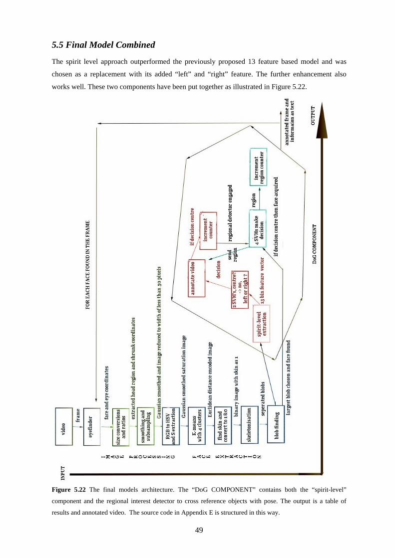
5.5 Final Model Combined
The spirit level approach outperformed the previously proposed 13 feature based model and was
chosen as a replacement with its added “left” and “right” feature. The further enhancement also
works well. These two components have been put together as illustrated in Figure 5.22.
Figure 5.22 The final models architecture. The “DoG COMPONENT” contains both the “spirit-level”
component and the regional interest detector to cross reference objects with pose. The output is a table of
results and annotated video. The source code in Appendix E is structured in this way.
49

Figure 5.23 shows and explains a snap shot of annotated video. A thorough evaluation of this final
model is conducted in the next Chapter where a precision of 89% is seen.
Regional interest detector. Gaze is inverted so it represents a billboard being faced by the
observer rather than the subject and is not laterally inverted.
Interest duration (secs) = total “looking” count ÷ 25fps
“Spirit-level” Component annotation for subject
looking “right”. (Laterally inverted) When faces are detected
this text appears and gives the verdict of looking and
not looking
If eyefinder finds a face then it is shown here. The frame count of the clip is
also shown here. Figure 5.23 Frame annotation explained.
50

Chapter 6: Evaluation Against Ground Truth The final model is thoroughly evaluated in this Chapter.
6.1 The Set Up
A detailed evaluation of the final system was carried out to ensure validity as well as verifiability
[2]. 1.5 hours of video footage was filmed from several locations with varying illumination,
elevation, background colour, and crowd trajectory angle to test the model for site installation
variance (Appendix E). Due to computational resource limitations requiring excessive time
consuming manual intervention the following decisions were made. From 1.5 hours of video footage
a few clips were created and processed totaling to approximately 4 minutes. Sample variations
within these clips are shown in Figure 6.1.
1 2 3 4 HIDDEN
FACE
HIDDEN FACE
5 6
HIDDEN FACE
7 8
HIDDEN FACE
Figure 6.1 Sample frames of the processed video clips. For the evaluation form; frame 1 is from clip “Khu”, 2
is from “Man”, 3 is from “Mich_proed”, 4 is from “sub_fork_proed”, 5 and 6 are from “stud_proed”, 7 is from
“sub_fork_40_60” and 8 is from “Close_up”. Frame 1 catered to a skin coloured background. Frame 7, for
example, represented posters inside tube stations between two path ways, and frame 3 represented a billboard
on a high rise.
It was not considered appropriate to compare the “interest duration” measure given by the model
with a manually timed one. A frame by frame analysis made a far better evaluation. With 25 frames-
per-second (fps) video clips and approximately 4 minutes of film, about 6000 frames would have
had to be manually annotated. This was not possible due to the time constraint, and a 2 second
interval (25 fps ∴ 50 frames for 2 seconds) was decided after observing how long individuals took
to change their DoG from objects of interest. 111 frames were obtained in this way. Due to
computational problems during processing, each interval of 50 frames does not tally with the actual
clip’s frame count. The completed evaluation form in Appendix I shows (from left to right) in each
row, the clip’s name (refer to Figure 6.1 for sample frames), a per clip frame count as on the clip
itself, a manual count from 1 to 5751 frames and classification information. Appendix E contains all
51

the extracted frames named with a concatenation of the clips name and the manual frame count, e.g.
Man_5601.jpg. The main evaluation criterion is precision accompanied by confusion matrix
information. Figure 6.2 provides an outline of the evaluation scheme followed and results follow.
MPT:eyefinder
True Face & Eyes
DoG DoG 3
False Face & Eyes
L R S Accept Reject
? 4
1
2
Figure 6.2 Evaluation scheme describing various parts of the model that have been evaluated. DoG represents
the proposed solution as in Chapter 5.
6.2 MPT’s Suitability
Stage 1 in Figure 6.2 shows the eyefinder. Although eyefinder is not the actual DoG model
proposed, it is part of the entire system and is therefore tested. 20 frames were selected from the
captured set, 1 to 501 and 2301 to 2801, and the total faces that lay between face poses C05 and C29
(Figure 3.1) were counted per frame (Appendix I). The first set of frames belonged to “Mich_proed”
and the second set belonged to “sub_fork_proed” (frame 3 and 7 from Figure 6.1 respectively). The
total faces were counted and those faces that appeared to be looking at the screen were also counted.
The faces ranged from 20 pixels to 40 pixels in height. These two separate counts were compared
with the actual correctly detected faces, (when eyefinder detects a face it also detects eyes). The
results are summarised in Table 6.1.
The first row in Table 6.1 represents a high location. MPT’s eyefinder detected only 17% of the
faces that were looking toward the simulated billboard or appeared close to pose C27 (Figure 3.1)
and only 4% of the faces in total. Frames 5 and 6 in Figure 6.1 illustrate this problem with no
detection or annotation visible. The other location yielded better but unsatisfactory results. The
totals favour eyefinder but a higher elevation installation is the most likely utilisation of this model.
Therefore when a better package is available it must replace MPT. Misclassifications were also a
problem. Figure 6.3 illustrates encountered misclassifications.
52

Raw Count Summary Percentage Location Actual
Count True Faces
Found Possible
C27’sActual Detection
Precision C27’s Detection
Precision“Mich_proed” 56 2 12 4% 17%
“sub_fork_proed” 36 14 12 39% 100% Totals 92 16 24 17% 67%
Table 6.1 Summary of MPT:eyefinder detection rate examination. For an elevated location (“Mich_proed”)
this face and eye detector was not acceptable. For a ground level and close proximity location it performed
better.
1 2 3 4
Figure 6.3 Frame 3, for example, shows a red arrow pointing to the left of the image plane. This is the
model’s answer to the eyefinder giving it an area of sky and leaves. The model proved to be robust in this way
dismissing most misclassifications. Frame 4 shows a misclassification being declared as “looking” due to very
little illumination which would have differentiated cloth from skin.
6.3 Robustness
Stage 2 in Figure 6.1 is a branch of the “False Face & Eyes”. The model is essentially a system
comprising of several SVM’s and other components. All systems possess the property of
emergence. Here the concept of emergence is seen in the system’s, or model’s, robustness. The
model should not be completely dependent on a face and eye detection package’s accuracy. For each
frame in the evaluation “True” and “False” face classifications were counted and the models
robustness. As shown in Appendix I, the total number of faces detected was 85 from 111 frames.
Out of those 85 faces 24 were misclassifications (Figure 6.3) so eyefinder had a 72% correct face
detection precision. The model classified 22 of these misclassifications as “not looking”, i.e., either
looking left or right, and 2 as “looking”. Therefore it is 92% (all figures rounded off) robust to input
from any face and eye detection package. This proves to be an imperative attribute that makes the
project commercially viable.
53

6.4 DoG Estimation Ability The following confusion matrices show how the model faired on an overall perspective.
Classification Truth Looking Not Looking
Looking 15 7 Not Looking 0 39
Table 6.2 With a 64% baseline an overall true positive and true negative precision of 89% was achieved to
cater to the minimum requirements.
Table 6.2 shows that the model has an overall combined, i.e. for all locations, classification
precision of 89% above a baseline of 64%. Individually positives were classified with a 68%
precision and negatives with a 100% precision. While the results were slightly biased toward the
negatives’, with an 89% overall precision expectations were exceeded.
In Table 6.2 “not looking” was a combination of “left” and “right” faces to measure how the model
dealt with its minimum requirement and thus verification [2] was completed. The left, right and
straight-on, feature, as described in Chapter 5, was added to complement the basic interest measure
of “looking” and “not looking” already catered to. As shown in Table 6.3, testing them separately
yielded good results. Classification
Truth Left Right Straight Left 7 12 0
Right 1 19 0 Straight 0 7 15
Table 6.3 Using “Right” for the Zero R baseline resulted in 33%. The overall truth in classification was 67%.
This added feature performed at 67% precision. Individually classifying images as “left” was 37%
accurate, “right” was 95% accurate and “straight-on” was 68% accurate. What the overall precision
did not show was that the model was biased toward classifying images as “right”. During training
the SVM had a bias toward a “right” classification and as discussed in Chapter 5 attempts were
made to deal with this to a certain level. It was not anticipated then that this was to cause problems.
Though, here there is a validated model performing at a reasonable precision overfitting is evident.
Since requirements verification was performed keeping elevations and locations in mind, a
validation for each location shown in Figure 6.1 is summarised in Table 6.5 from Appendix I.
Stage 4 involves evaluating the regional interest feature. Since it was not possible, within the
projects schedule, to perform a detailed evaluation here by counting negatives and positives for each
54

region a binary decision is given. Figure 6.4 illustrates how the decision is made. Table 6.4
summarises the regional interest gauge evaluation results.
Mich_proed Classification Classification Truth Left Right Straight Truth Looking Not Looking Left 6 1 0 Looking 5 0
Right 0 2 0 Not Looking 0 9 Straight 0 0 5
sub_fork_proed Classification
Truth Left Right Straight Classification Left 0 2 0 Truth Looking Not Looking
Right 1 6 0 Looking 3 3 Straight 0 3 3 Not Looking 0 9
sub_fork_40_60 Classification
Truth Left Right Straight Classification Left 0 4 0 Truth Looking Not Looking
Right 0 8 0 Looking 1 3 Straight 0 3 1 Not Looking 0 12
Khu Classification
Truth Left Right Straight Classification Left 0 0 0 Truth Looking Not Looking
Right 0 0 0 Looking 1 0 Straight 0 0 1 Not Looking 0 0
Close_up Classification
Truth Left Right Straight Classification Left 1 0 0 Truth Looking Not Looking
Right 0 1 0 Looking 3 1 Straight 0 1 3 Not Looking 0 2
stud_proed Classification
Truth Left Right Straight Classification Left 0 5 0 Truth Looking Not Looking
Right 0 0 0 Looking 2 0 Straight 0 0 2 Not Looking 0 5
Man Classification
Truth Left Right Straight Classification Left 0 0 0 Truth Looking Not Looking
Right 0 2 0 Looking 0 0 Straight 0 0 0 Not Looking 0 2
Table 6.3 A summary break up per location is presented in the confusion matrices, produced from Appendix
I. The minimum feature is presented in the confusion matrices running along the right and the added “left”,
“right” and “straight-on” feature is shown on the left. The name of each clip is provided.
55

1 2
HIDDEN FACE
HIDDEN FACE
4 3
Figure 6.4 Frame 1 and 2 show mistakes. In 1 the frame is confusing and so the model classified it as
“looking at region 2”. In frame 2 the subject is looking straight towards region 5 rather than region 4 as
classified. These two are considered as “False” in the evaluation form. Frames 3 and 4 correctly identify
possible regions of gaze and therefore are considered as “True”.
Regional
Location TRUE FALSE Mich_proed 5 0
Khu 1 0 sub_fork_proed 2 1
Close_up 1 2 sub_fork_40_60 0 1
stud_proed 1 1 Man 0 0
Table 6.4 Summary of regional interest detector for each location. Showing specifically that for the elevated
high position that it should cater to (“Mich_proed”) it performed 100 % correctly.
Table 6.5 summarises the combined final systems precision per location and Figure 6.5 illustrates
these values.
56

Direction of Gaze Model Features Location LRS Yes or No Regional
Mich_proed 93% 100% 100% Khu 100% 100% 100%
sub_fork_proed 60% 80% 67% Close_up 83% 83% 33%
sub_fork_40_60 56% 81% 0% stud_proed 29% 100% 50%
Man 100% 100% 0% Totals 67% 89% 67%
Table 6.5 Precision of all features at all locations. LRS is the “left”, “right” and “straight-on” component,
“Yes or No” is the minimum “looking” or “not looking” component and “Regional” represents the regional
interest detector.
9 3 %10 0 %
6 0 %
8 3 %
56 %
2 9 %
6 7%
10 0 % 10 0 %
8 0 %8 3 % 8 1%
10 0 %
8 9 %
10 0 %
6 7%
3 3 %
0 %
50 %
0 %
10 0 %
10 0 %
10 0 %
6 7%
0 %
10 %
2 0 %
3 0 %
4 0 %
50 %
6 0 %
70 %
8 0 %
9 0 %
10 0 %
Mich_p
roed
Khu
sub_
fork_
proed
Close_
up
sub_
fork_
40_60
stud_
proe
dMan
Total
s
TR U E Y es or N o R eg io nal
Figure 6.5 Visualisation of Table 6.5. The entire system performs very well on “Mich_proed” and on a skin
coloured background of “Khu”. For a ground level application, “sub_fork” it is also suitable but for a close up
with a very large face it is affected by the location of the eyes since they are more precisely found by MPT’s
eyefinder. The regional interest measure has also proved to be working well in a number of settings other than
the high level. The totals suggest an all rounding satisfactory performance.
57

6.5 Evaluation Summary As with any evaluation it is only possible to reveal the presence of errors rather than their absence
[3]. This is the motivation behind the methodology chosen. The evaluation technique used was
hoped to be least biased and at the same time convenient. That is, if frames were manually selected
then automatically preference would have been given to those that favour the model, and if a
random frame grabber was programmed then time consuming computational resource problems
would have been faced. However the scheme had the drawback of not giving a good idea of smaller
video clips such as “Khu” for a skin coloured background and “Man” for a cluttered background
and single subject outdoor analysis.
The skin coloured background was problematic (refer to “Khu.wmv” in Appendix E) only for
robustness and classifications were otherwise accurate owing to a saturation based segmentation
technique. Other than this the major problem was MPT which though is based on the state-of-the-art
Viola-Jones model, is error prone. It has a particularly discouraging problem of not being able to
detect dark skinned subjects unless in ideal illumination conditions. Other factors also apply that
have already been looked at in detail.
Despite component problems, the model performed very well. It is robust and accurate on a number
of sites including the high elevation that it was supposed to perform well on. The overall precision
was 89% for the simple minimum requirements and 67% for the added “left”, “right” and “straight-
on” feature. The “spirit-level” model had a lower accuracy of 78% in the controlled environment.
The “left or right” feature suffered from the SVM bias of a “right” classification which caused the
decline from the controlled environment testing result of 84% thus showing over-fitting and
optimisation. However it is better to have a system that is biased toward the “not looking” side to
suppress the interest gauge rather than show an overly exaggerated result. The regional interest
measure also performed extremely well but showed a decline from the controlled laboratory test-set
environment of 77% to a 67% accuracy or precision. Though this is lower it is still a satisfactory
result.
As demonstrated, a cognitive vision model to gauge interest in advertising hoardings was
successfully developed. Even if precisions are not at 100%, the model can be used not only to gauge
interest in particular advertisements but also to compare advertisements and in several other
applications.
58

Chapter 7: Future Work Possible additions to this project are discussed here.
This project provided a platform for a number of possible extensions. Among the two further
enhancements expression recognition could not be explored mainly to keep within the projects
schedule. Other concerns included the possibilities of heads being too small in footage from high
hoardings so facial expressions would not have been exploitable. However, during the development
it was realised that the heads will usually be big enough to get a rough approximation of the
subject’s expression. Though Figure 7.1 was taken from 40 feet above ground level and the image is
enlarged, super-sampling with interpolation methods can be used to clear up tiny distorted faces to
classify their expressions. The PIE database that has already been acquired and discussed can easily
be used for its expression images. Besides this body speed and trajectory, and posture and head
gestures including nods can complement an expression matching system. Such techniques are
important because it is not likely to have most of the pedestrian reactions shown in Figure 7.2.
These subjects appear to be
smiling
Figure 7.1 Example frame from height showing that expressions in heads 20 pixels high are still visible.
Figure 7.2 Unlikely and ideal facial expressions for a facial expression recognition model. Source [60]
The literature review has already covered techniques for trajectory and velocity incorporation using
Markov models and other probabilistic methods [25]. Other interest cues can be developed. For
example, if a subjects head has turned a considerable pan off the body’s trajectory for an extended
period of time this shows greater interest and goes beyond the current model. For this tracking
techniques need to be developed. There are several other possible extensions. Linking the system to
a National Identification or Drivers License database and adding a face recognition system to study
what demographics show the most interest would help pricing, market penetration and also
inventory control. As a first step, though, PCA should be used with the saturation based
segmentation technique to extract a perfect head. In this way, the regional detector can also be made
more precise. Although non-model approaches were to be tried it is only beneficial to incorporate a
model based approach beyond the ellipses as this project has been completed.
59

Chapter 8: Conclusion The reports conclusion
The need to develop a system that gauged interest in advertisement hoardings existed and for this a
system was developed. Proposed is a cognitive vision model to gauge interest in advertisement
hoardings. This technique of using pin point “spirit-level” binary feature vectors combined with a
regional detector is very useful in a number of settings apart from media research and advertising. It
can be used in HCI, for which many systems have been devised, gaze-navigation systems and
human robot interaction such as that used in [23].The model proved to work very well as shown in
Chapter 6 with an 89% accuracy exceeding all expectations. During the projects course several new
techniques were explored and the final model too is novel. It is hoped that this model and its
documentation will provide a useful platform and study for future gaze estimation research in multi-
resolution video.
60

References All citations within the text are listed here.
[1] The Advertising Association, (2006), Advertising Statistics Yearbook 2006, WARC.
[2]Sommerville I, (2000), Software Engineering, 6th Edition, Addison-Wesley.
[3]Sommerville I, (2004), Software Engineering, 7th Edition, Pearson/Addison-Wesley.
[4] Sim T, Baker S, Bsat M, (2002), The CMU Pose, Illumination, and Expression (PIE)
Database, in Proceedings of the International Conference on Automatic Face and Gesture
Recognition.
[5]Checkland P, (1981), Systems Thinking Systems Practice, Wiley.
[6 ] The American Heritage, (2000), Dictionary of the English Language, 4th edition, Houghton
Mifflin Company.
[7] WordNet, (2003), version 2.0, Princeton University.
[8] Pomberger G, Blaschek G, (1996), Object orientation and prototyping in software engineering,
translated by Bach R, Prentice Hall.
[9] Forsyth D, Ponce J, (2003), Computer Vision: A Modern Approach, Prentice Hall.
[10] Ramaswami S, Kim J, Bhargava M, (2001) Advertising productivity: developing an agenda for
research, in the International Journal of Advertising, vol. 20, no. 4.
[11] Franke G, Taylor C, (2003) Business perceptions of the role of billboards in the U.S. economy,
in the Journal of Advertising Research, vol. 43, no. 2, June 2003.
[12] McEvoy D, (2002) Outdoor: the Creative Medium, Admap, May 2002, Issue 428
[13] Coleman R, Cunningham A, (2004),Outdoor advertising recall: A comparison of newer
technology and traditional billboards, in ESOMAR, Online and Outdoor Conference, Geneva.
[14] Advertising Standards Authority, (2002), Outdoor Advertising Survey 2002: Compliance
Report, [Online] [Accessed: 7th August 2006] URL: http://www.asa.org.uk/NR/rdonlyres/A5F2E70F-
8661-4D06-8284 5726DFC296AF/0/ASA_Poster_Research.pdf
[15] Kerne A, Jumboscope Group, JumboScope: A Site-Specific Installation and Platform, [online]
[Accessed 11th August 2006] URL: http://www.cs.tufts.edu/colloquia/colloquia.php?event=169
[16] Kerne A, (1997), Collage Machine: Temporality and Indeterminacy in Media Browsing via
Interface Ecology, in the Proceedings of the ACM SIGCHI Conference on Human Factors in
Computing Systems Extended Abstracts, pp. 297-298, March 1997.
[17] Boyland M, Janes I, Barber H, (2004), The full picture, ESOMAR, Technovate 2, Barcelona.
[18] Krugman D, Fox R, Fletcher J, Fischer P, Rojas T, (1994), Do Adolescents Attend to Warnings
in Cigarette Advertising? An Eye-Tracking Approach, in the Journal of Advertising Research,
vol. 34, no. 6, November/December 1994.
[19] Heinzmann J, Zelinsky A, (1998) 3-D facial pose and gaze point estimation using a robust
real-time tracking paradigm, in the Proceedings of the 3rd IEEE International Conference on
Automatic Face and Gesture Recognition. pp.142-147, April 1998.
61

[20] Gee A, Cipolla R, (1994), Estimating gaze from a single view of a face, in the Proceedings of
the 12th IAPR International Conference on , vol.1, pp.758-760 October 1994.
[21] Morimoto C, Amir A, Flickner M, (2002) Detecting Eye Position and Gaze from a Single
Camera and 2 Light Sources, in the Proceedings of the 16th International Conference on
Pattern Recognition (ICPR'02). vol. 4. pp. 40314.
[22] Wang J.-G, Sung E, Venkateswarlu R, (2003) , Eye gaze estimation from a single image of one
eye, in the Proceedings of the Ninth IEEE International Conference, vol., no.pp. 136- 143 vol.1,
13-16 October 2003.
[23] Nagai Y, (2005), The Role of Motion Information in Learning Human-Robot Joint Attention, in
the Proceedings of the 2005 IEEE International Conference on. pp. 2069- 2074 April 2005.
[24] Voit M, Nickel K, Stiefelhagen R, (2005), Multi-view face pose estimation using neural
networks, , in the Proceedings of the 2nd Computer and Robot Vision Canadian Conference on
, pp. 347- 352, May 2005.
[25] Robertson N, Reid I, Brady J, (2005), What are you looking at? Gaze estimation in medium-
scale images, in the Proceedings of HAREM 2005.
[26] Castrillon-Santana M, Deniz-Suarez O, Guerra-Artal C, Hernandez-Tejera M, (2005), Realtime
Detection of Faces in Video Streams, in the Proceedings of the 2nd Canadian Conference on
Computer and Robot Vision (CRV'05), pp. 298-305.
[27] Viola P, Jones M, (2003), Fast Multi-View Face Detection, Mitsubishi Electric Research
Labs, Demonstration at the IEEE Conference on Computer Vision and Pattern Recognition
(CVPR'03).
[28] Viola P, Jones M, (2001), Rapid object detection using a boosted cascade of simple features, in
Proceedings of the IEEE Conference on Computer Vision and Pattern Recognition, Kauai, HI.
[29] Machine Perception Laboratory. [online] [Accessed 9th June 2006] URL:
http://mplab.ucsd.edu:16080/
[30] Benoit A, Bonnaud L, Caplier A, Ngo P, Lawson L, Trevisan D, Levacic V, Mancas C, Chanel
G,- (2005), Multimodal Focus Attention Detection in an Augmented Driver Simulator, in
Proceedings of eNTERFACE’ 05 workshop, Mons, Belgium.
[31] Tasaki T, Komatani K, Ogata T, Okuno H.G, (2005), Spatially mapping of friendliness for
human-robot interaction," in Proceedings of IEEE/RSJ International Conference on Intelligent
Robots and Systems (IROS 2005). pp. 1277- 1282.
[32] Hand D, Mannila H, Smyth P, (2001), Principles of Data Mining (Adaptive Computation and
Machine Learning), MIT Press.
[33] Mitchell T, (1997), Machine Learning, McGraw-Hill.
[34] Beal R, Jackson T, (1990) Neural Computing: An Introduction, IOP Publishing Ltd.
[35] DTREG, SVM - Support Vector Machines [online] [Accessed 13th August 2006]
URL:http://www.dtreg.com/svm.htm
[36] Donald S, (2000) , Statistics: a first course, 6 Edition, th McGraw-Hill.
62

[37] Cytel Statistical Software, XLminerTM Online Help, Version 3, [online] [Accessed 13th August
2006] URL: http://www.resample.com/xlminer/help/rtree/rtree_intro.htm
[38] Manning C, Schuetze H, (1999). Foundations of Statistical Natural Language Processing, MIT
Press.
[39] Markert K, Language: Semantic Similarity, [online] [Accessed 13th August 2006] URL:
http://www.comp.leeds.ac.uk/lng/lectures/handout3.pdf
[40] Leibe B, Schiele B, (2003) Interleaved Object Categorization and Segmentation. in
Proceedings of the British Machine Vision Conference (BMVC'03).
[41] Anderson P, (2005), Object Recognition Using An Interest Operator, [online] [Accessed 16th
April 2006] URL: http://www.comp.leeds.ac.uk/fyproj/reports/0405/AndersonP.pdf
[42] Dang M, Choudri S, (2006) Simple Unsupervised Morphology Analysis Algorithm (SUMAA),
in Proceedings of the PASCAL Challenge Workshop, Venice.
[43] Hogg D, (2006), Computer Vision: Lecture slides, University of Leeds, [online] [Accessed 16th
April 2006] URL: http://www.comp.leeds.ac.uk/vsn/
[44] Stauffer C, Grimson W, (1999) Adaptive background mixture models for real-time tracking, in
Computer Vision Pattern Recognition, pp. 246—252.
[45] Vision Group, Leeds University, ftp://smb.csunix.leeds.ac.uk/home/cserv1_a/ssa/vislib/
[46] Pomerleau D, (1989), ALVINN: An autonomous land vehicle in a neural network, in D.S.
Touretzky, editor, Advances in Neural Information Processing Systems, vol. 1, pp. 305-313,
[47] Gonzalez R, Woods R, Eddins S, (2003), Digital Image Processing Using MATLAB, 1st
Edition, Prentice Hall.
[48] Brooks R, (1991), Intelligence Without Reason, in Proceedings of the 12th International
Joint Conference on Artificial Intelligence Sydney Australia, August 1991, pp. 569–595.
[49] UK MSN, [online] [Accessed 16th April 2006] URL: http://uk.msn.com/
[50] Fisher R, Perkins S, Walker A, Wolfart E, The Hypermedia Image Processing Reference,
University of Edinburgh, [online] [Accessed 1st August 2006] Available from URL:
http://homepages.inf.ed.ac.uk/rbf/HIPR2/
[51] Choudri S, (2006), RoSo2 algorithm for Texture Segmentation, Computer Vision: Coursework.
[52] Dance C, Willamowski J, Fan L, Bray C, Csurka G, (2004), Visual categorization with bags of
keypoints. in the Proceedings of ECCV International Workshop on Statistical Learning in
Computer Vision.
[53] Gonzalez, R, Woods R, Eddins S, (2004), Digital Image processing using MATLAB, Upper
Saddle River, NJ, Pearson/Prentice Hall.
[54] Hanselman D, (2005) Ellipsefit.m, University of Maine, Orono, ME 04469 Mastering
MATLAB 7 [online] [Accessed 22nd August 2006] URL:
http://www.mathworks.com/matlabcentral/files/7012/ellipsefit.m
[55]Halif R, Flusser J, (2000), Numerically Stable Direct Least, Squares FItting of Ellipses,
Department of Software Engineering, Charles University, Czech Republic.
63

[56] Lei Wang, (2003), ellipsedraw.m, [online] [Accessed 22nd August 2006] URL:
http://www.mathworks.com/matlabcentral/files/3224/ellipsedraw.m
[57] Google images, [online] [Accessed 22nd August 2006]URL:
http://images.google.co.uk/images?svnum=10&hl=en&lr=&q=coke+billboard&btnG=Search
[58] Young D, Computer Vision: Lecture slides, University of Sussex, [online] [Accessed 10th July
2006] URL: Computer http://www.cogs.susx.ac.uk/courses/compvis/slides_lec5.pdf
[59] Forbes K, Some Simple Image Processing Tools for Matlab, [online] [Accessed 10th July 2006]
URL: http://www.dip.ee.uct.ac.za/~kforbes/KFtools/KFtools.html
[60] Essa I, Pentland A, (1995), Facial Expression Recognition Using a Dynamic Model and Motion
Energy, in the Proceedings of ICCV.
64

Appendix A: Reflection A reflection of experience that should be beneficial to other students in the future. While it is not possible to cover all the experience gained some aspects should be useful for others
to learn from. With any problem the simplest of solutions should be exhausted first. The image
segmentation techniques that were tried tended to be overly complicated at times when the actual
solution settled on was extremely simple to implement. For example, if simple experimentations
with RGB and HSV images had been exhausted earlier the further enhancement of expression
recognition could have been developed or more time could have been spent evaluating more frames.
Possible additions to a saturation based technique include using the mean-shift tracker. Without
using a PCA model those two techniques should give fruitful results in symbiosis.
The development environment is a very important aspect with any computer science problem.
Matlab provided rapid prototype development capabilities but also has poor memory management.
It is essential to keep such factors in mind since this project suffered considerably as a result. It took
2 weeks to manage to successfully process film that was expected to take a few days. Finally 1.5
hours of video was reduced to clips of 1 minute each which took at least half a day to compute. The
other alternative was to use OpenCV libraries and code in C++ but experience suggested that Matlab
was simpler. The lesson here is that if high quality images are to be processed (frames) then RAM
greater than 1GB is required. After every 80 frames (1024x786 pixel dimensions) of a 1 minute AVI
clip (approx.100MB) the system would crash with 1GB RAM. Also the task was divided among 4
computer systems with Intel Pentium 4 processors of 2.8 GHz, each with atleast 50 GB of hard disk
space for virtual memory. The higher resolution was essential to be able to detect smaller heads. The
computers were limited to 4 since the Matlab release being used had license limitations for its image
processing toolbox. This was another problem that should be kept in mind while developing
systems. Since this is an idea converted to a project there were certain aspects that were both pros
and cons. Firstly there was no set specification that allowed the development process to use as a
milestone and there was no existing system to beat. This also meant possible “feature-creep”.
However, at the same time it prevented “feature-creep” since there was no representative from the
industry and allowed development in a very research oriented style. The aspect governing its
success was a clearly defined precise set of minimum requirements from the very start and a specific
evaluation criteria to measure success with. While still on the subject of “idea to a project” it is
important to define an achievable schedule with large buffers in place. Since this is mainly a self-
driven project such buffers are required. For example, in July the development finished as planned
but the evaluation portion used up the buffer due to problems discussed. Lastly, for the report it is
important to document and evaluate everything during development and keep code to reproduce
results.
65

Appendix B: Objectives and Deliverables Form Objectives and deliverables form recording the initial agreement of minimum requirements, deliverables and other aspects of the project.
AIM AND REQUIREMENTS FORM COPIED TO SUPERVISOR AND STUDENT ---------------------------------------------------------- Name of the student: Saad CHOUDRI Email address: scs5sc Degree programme: MCGS - MSc in Cognitive Systems Number of credits: 60 Supervisor: dch Company: (none) The aim is: Development of Computer Vision concepts and skills through experience. The project outline is: Background reading: Reading and understanding face and gesture recognition to understand models such as the Viola and Jones model. Methodology: Prototype Development Product: Software implementation Evaluation of product: Performance evaluation against ground truth. The minimum requirements are: 1. Integrate off the shelf face and eye detection software 2. Estimate viewing direction from a face and eye detection package augmented with novel algorithms and or, approaches through literature research. 3. Devise a measure of interest from viewing angle and duration of viewing. 4. Evaluate the system documented in a report. 5. Enhancement Optionals 1) incorporate facial expression into the interest measure 2)Cross reference objects in the display to gauge level of interest in object. The hardware and software resources are: 1. Video Cameras from Vision Lab 2. Extra disk space as needed on school computers, starting with about 100 MB. 3. Continuous Mat Lab availability and support on school computers. The foundation modules are: 1. COMP5430M 2. COMP5420M The project title is Cognitive Model gauging interests in advertising hoardings.
66

Appendix C: Marking Scheme and Header Sheet The marking scheme, header sheet and comments from the interim report are give below.
67

68 68

69

Appendix D: Gantt Chart and Project Management Reflection on the project management and updates are given below Schedule Feb Mar Apr May Jun Jul Aug Sep Background Reading 1 2 3 4 1 2 3 4 1 Concurrent activities Final Evaluation Poster Report Free slots for delays KEY Completion of 3 stages and 1 week off. Project submission.
Table 1 Original Schedule describing an overview of the planned assigned weeks. For example the whole of
June was to take up the concurrent activities and background reading but only the first 3 weeks of August
were to be used for report writing. The key describes irregularities.
Schedule Feb Mar Apr May Jun July Aug Background Reading 1 2 3 4 1 2 3 4 Concurrent activities Done Final Evaluation Ongoing Poster Report Free slots for delays KEY Completion of 3 stages and 1 week off.
Project submission.
18th July progress meeting.
Table 2 Schedule as on 18th July.
The final evaluation stage threw the project off track and processing continued till the 10th of August
due to lack of resources such as RAM. This delayed all the other activities but the 1st and 2nd drafts
of the entire report were done by the 31st of August and so the buffer zones were very useful and
well planned.
A total of 280 hours of solid productive work were required for the evaluation troubleshooting,
report writing and poster making during August and the entire project was ready for submission 5
days before the deadline, on the 1st of September. Prior to this at least 400 hours were spent since
February. Therefore a total of 640 hours were spent productively for this project.
70

Appendix E: CD All deliverables other than this report, images, videos etc and source code are in the CD enclosed with the printed report handed in on the 6th of September 2006.
The following points explain how to use this CD or Appendix E (E for electronic). A readme.txt file
per section is present explaining the contents. The sections are:
• The folder titled “Deliverables” includes
o Evaluation videos filmed ( edited and as many as could fit on the CD)
o Processed clips ( named in accordance with evaluation form)
o Extracted Frames that were evaluated manually.
o Software code with workspace and usage instructions. (demonstration arrangeable)
• The folder titled “Dataset” contains
o All the training images, testing images, and extra 70 images taken for
The main DoG Component
The further enhancement
MPT testing
• The folder titled “Miscellaneous” contains
o Histograms etc. to understand the parameters of the 13 feature approach
o Background, skin and hair pictures
71

Appendix F: Dataset This Appendix contains thumbnails of the training and test images.
Figure F.1 Training images. 34 centre, 19 left and 20 right facing images. Subjects with glasses and without
glasses have been repeated in some areas. Other images have also been included to avoid optimisation.
Figure F.2 68 “looking” images selected on the basis of appearance variation. Some images have been
repeated to see how classifiers behave with previously seen images as well as unseen.
72

Figure F.3 65 “not looking” test images. Carefully selected images with many unseen poses, varying
appearance, illumination, background and expression, and that are likely to be misclassified.
Figure F.4 Training images for cross referencing objects with pose. 5 different poses used as described.
Figure F.5 Test images for cross referencing objects with pose. Carefully selected subjects with varying
appearance.
73

Appendix G: 13 Feature Analysis Samples Histograms and range analysis for Normal distribution.
L=left, R=right, S=straight or centre, Y=looking, N= not looking
Figure G.1 FCX
Figure G.2 FCY
Figure G.3 REY
This was a subset of the 13 histograms for L R and S that were plotted. The rest may be found in
Appendix E. Following are the same histograms but as yes and no rather than left right and straight.
74

Figure G.4 FCX
Figure G.5 FCY
Figure G.6 REY
The rest of the set of histograms are in Appendix E.
75

Appendix H: Image Segmentation Samples Screen shots of the various implemented image segmentation techniques on 76 training images.
Figure H.1 Face and hair extraction using K-means and Euclidean distance with 3 clusters for the background
and 2 for the subject.
Figure H.2 Results of encoding using 5 Gaussians. Equal probabilities are the biggest problem.
76

Figure H.3 6 Gaussians, 3 for face and 3 for background and used for joint probability.
Figure H.4 The foreground and background pixels individually representing 2 Gaussians
77

Figure H.5 An adaptive background approach using a series of Gaussians.
Figure H.6 After 3 iterations of the adaptive accumulative Gaussian approach from Figure H.5.
78

Figure H.7 Texture segmented images
Figure H.8 Ellipse on texture without adjustments
79

Figure H.9 Ellipse fit on RGB images
Figure H.10 Ellipse on texture with adjustments. The ellipse has been drawn on the original images but with
the coordinates of the textured image.
80
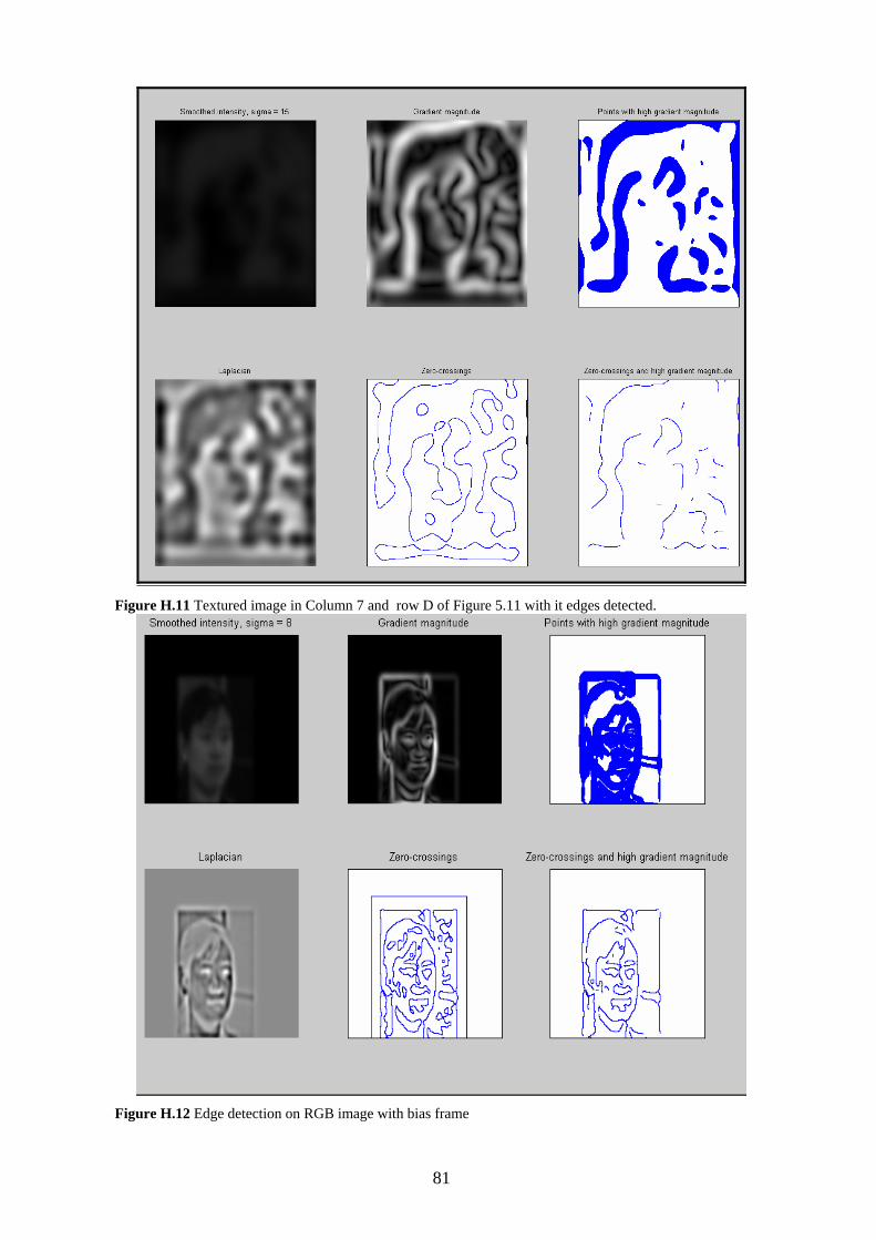
Figure H.11 Textured image in Column 7 and row D of Figure 5.11 with it edges detected.
Figure H.12 Edge detection on RGB image with bias frame
81

Figure H.13 Training image subset in saturation method with ellipses to show the colour discrimination.
Figure H.14 Faces segmented using saturation and K-means.
82

Appendix I: Ground Truth Evaluation Form Completed Evaluation form for 111 frames as described in Chapter 6. The empty cells are equivalent to zeros and were not required to be filled.
KEY Left-Right-Straight-True-False-NotLooking-Looking
Correct Classification Misclassification
Not Looking Looking
Frame Information Left Right Straight Region
Eyefinder Detection Precision
CVMGIAH
Robustness
Clip Frame No. L R S L R S L R S T F T F N L
Mich_proed 1 1 1 0 0 0 0 0 0 0 0 0 0 1 0 0 0
Mich_proed 50 51 0 0 0 0 0 0 0 0 0 0 0 0 0 0 0
Mich_proed 101 101 0 0 0 0 0 0 0 0 0 0 0 0 0 0 0
Mich_proed 151 151 0 0 0 0 0 0 0 0 0 0 0 0 1 1 0
Mich_proed 201 201 0 0 0 0 0 0 0 0 0 0 0 0 1 1 0
Mich_proed 251 251 0 1 0 0 0 0 0 0 0 0 0 1 0 0 0
Mich_proed 301 301 0 0 0 0 0 0 0 0 0 0 0 0 0 0 0
Mich_proed 351 351 0 0 0 0 0 0 0 0 0 0 0 0 0 0 0
Mich_proed 401 401 0 0 0 0 0 0 0 0 0 0 0 0 0 0 0
Mich_proed 450 451 0 0 0 0 1 0 0 0 0 0 0 1 2 1 1
Mich_proed 501 501 0 0 0 0 0 0 0 0 0 0 0 0 0 0 0
Mich_proed 551 551 0 0 0 0 0 0 0 0 1 1 0 1 0 0 0
Mich_proed 601 601 1 0 0 0 0 0 0 0 0 0 0 1 0 0 0
Mich_proed 651 651 0 0 0 0 0 0 0 0 0 0 0 0 1 1 0
83

Mich_proed 701 701 1 0 0 0 0 0 0 0 0 0 0 1 0 0 0
Mich_proed 750 751 1 0 0 0 0 0 0 0 0 0 0 1 0 0 0
Mich_proed 801 801 0 0 0 0 0 0 0 0 0 0 0 0 0 0 0
Mich_proed 851 851 0 0 0 0 0 0 0 0 1 1 0 1 0 0 0
Mich_proed 901 901 0 0 0 0 0 0 0 0 1 1 0 1 0 0 0
Mich_proed 950 951 0 0 0 0 1 0 0 0 0 0 0 1 1 1 0
Mich_proed 1001 1001 0 0 0 0 0 0 0 0 0 0 0 0 1 1 0
Mich_proed 516 1051 0 0 0 0 0 0 0 0 0 0 0 0 0 0 0
Mich_proed 567 1101 0 0 0 0 0 0 0 0 0 0 0 0 0 0 0
Mich_proed 1174 1151 1 0 0 0 0 0 0 0 1 1 0 2 0 0 0
Mich_proed 1225 1201 0 0 0 0 0 0 0 0 0 0 0 0 1 1 0
Mich_proed 1276 1251 0 0 0 0 0 0 0 0 0 0 0 0 0 0 0
Mich_proed 1327 1301 0 0 0 0 0 0 0 0 0 0 0 0 0 0 0
Mich_proed 1377 1351 1 0 0 0 0 0 0 0 1 1 0 2 0 0 0
Mich_proed 1428 1401 0 0 0 0 0 0 0 0 0 0 0 0 1 1 0
Mich_proed 1478 1451 0 0 0 0 0 0 0 0 0 0 0 0 1 1 0
Mich_proed 1528 1501 0 0 0 0 0 0 0 0 0 0 0 0 0 0 0
Mich_proed 1578 1551 0 0 0 0 0 0 0 0 0 0 0 0 1 1 0
Mich_proed 1628 1601 0 0 0 0 0 0 0 0 0 0 0 0 1 1 0
Mich_proed 1678 1651 0 0 0 0 0 0 0 0 0 0 0 0 0 0 0
Mich_proed 1728 1701 0 0 0 0 0 0 0 0 0 0 0 0 1 1 0
84

Khu 212 1751 0 0 0 0 0 0 0 0 1 1 1 0 0 0
Khu 204 1801 0 0 0 0 0 0 0 0 0 0 0 0 0 0 0
Khu 312 1851 0 0 0 0 0 0 0 0 0 0 0 0 0 0 0
Khu 302 1901 0 0 0 0 0 0 0 0 0 0 0 0 0 0 0
Khu 412 1951 0 0 0 0 0 0 0 0 0 0 0 0 0 0 0
Khu 404 2001 0 0 0 0 0 0 0 0 0 0 0 0 0 0 0
sub_fork_proed 5 2051 0 0 0 0 0 0 0 0 0 0 0 0 0 0 0
sub_fork_proed 55 2301 0 1 0 0 2 0 0 0 1 1 0 4 0 0 0
sub_fork_proed 147 2351 0 0 0 0 0 0 0 0 1 1 0 1 1 1 0
sub_fork_proed 198 2401 0 0 0 0 0 0 0 0 0 0 0 0 0 0 0
sub_fork_proed 248 2451 0 0 0 1 0 0 0 0 0 0 0 1 0 0 0
sub_fork_proed 298 2501 0 0 0 0 0 0 0 0 0 0 0 0 0 0 0
sub_fork_proed 348 2601 0 0 0 0 2 0 0 0 0 0 0 2 1 1 0
sub_fork_proed 398 2651 0 0 0 0 2 0 0 1 1 0 1 4 1 1 0
sub_fork_proed 448 2701 0 1 0 0 0 0 0 1 0 0 0 2 0 0 0
sub_fork_proed 498 2751 0 0 0 0 0 0 0 0 0 0 0 0 0 0 0
sub_fork_proed 548 2801 0 0 0 0 0 0 0 0 0 0 0 0 0 0 0
sub_fork_proed 598 2851 0 0 0 0 0 0 0 1 0 0 0 1 1 1 0
85

Close_up 1 2901 0 0 0 0 0 0 0 0 1 0 1 1 0
Close_up 50 2951 1 0 0 0 0 0 0 0 0 0 0 1 0
Close_up 101 3001 0 0 0 0 0 0 0 0 1 1 0 1 0
Close_up 151 3051 0 0 0 0 1 0 1 0
Close_up 200 3101 0 0 0 0 0 0 0 0 0 0 0 0 0 0 0
Close_up 251 3151 0 0 0 0 0 0 0 0 0 0 0 0 0 0 0
Close_up 301 3201 0 0 0 0 0 0 0 0 0 0 0 0 0 0 0
Close_up 351 3251 0 0 0 0 0 0 0 0 0 0 0 0 0 0 0
Close_up 401 3301 0 0 0 0 0 0 0 1 0 0 0 1 0 0 0
Close_up 450 3351 0 0 0 0 0 0 0 0 1 0 1 1 0 0 0
0
sub_fork_40_60 1 3401 0 0 0 0 0 0 1 1 0 1 2 0
sub_fork_40_60 51 3451 0 0 0 0 2 0 1 0 3 0
sub_fork_40_60 101 3501 0 1 0 0 1 0 0 2 0
sub_fork_40_60 151 3551 0 0 0 0 1 0 0 1 0
sub_fork_40_60 201 3601 0 0 0 0 0 0 0 0 0 0 0 0 0 0 0
sub_fork_40_60 251 3651 0 0 0 0 2 0 0 2 0
sub_fork_40_60 301 3701 0 0 0 0 0 0 0 0 0 0 0 0 0 0 0
sub_fork_40_60 351 3751 0 0 0 0 0 0 0 0 0 0 0 0 0 0 0
sub_fork_40_60 401 3801 0 0 0 0 0 0 0 0 0 0 0 0 0 0 0
sub_fork_40_60 451 3851 1 0 1 0
sub_fork_40_60 501 3901 0 0 0 0 0 0 0 0 0 0 0 0 0 0 0
86

sub_fork_40_60 551 3951 0 0 0 0 0 0 0 0 0 0 0 0 0 0 0
sub_fork_40_60 701 4001 0 0 0 0 1 0 0 0 0 0 0 1 0 0 0
sub_fork_40_60 751 4051 0 2 0 0 1 0 0 0 0 0 0 3 1 1
sub_fork_40_60 801 4101 0 1 0 0 0 0 0 0 0 0 1 0
sub_fork_40_60 851 4151 0 0 0 0 0 0 0 0 0 0 0 0 0 0 0
0 0 0 0 0 0 0 0 0 0
stud_proed 1 4201 0 0 0 0 0 0 0 0 0 0 0 0 0 0 0
stud_proed 51 4251 1 1 1 1
stud_proed 101 4301 0 0 0 0 0 0 0 0 0 0 0 0 0 0 0
stud_proed 151 4351 0 1 0 0 0 0 0 0 0 0 0 1 0
stud_proed 201 4401 0 2 0 0 0 0 0 0 0 0 0 2 0
stud_proed 251 4451 0 0 0 0 0 0 0 1 0 1 1 0
stud_proed 301 4501 0 0 0 0 0 0 0 1 1 0 1 1 1
stud_proed 351 4551 0 0 0 0 0 0 0 0 0 0 0 0 0 0 0
stud_proed 401 4601 0 1 0 0 0 0 0 0 0 0 0 1 0 0 0
stud_proed 451 4651 0 0 0 0 0 0 0 0 0 0 0 0 0 0 0
stud_proed 501 4701 0 0 0 0 0 0 0 0 0 0 0 0 0 0 0
stud_proed 551 4751 0 0 0 0 0 0 0 0 0 0 0 0 1 1
stud_proed 601 4801 0 0 0 0 0 0 0 0 0 0 0 0 0 0 0
stud_proed 651 4851 0 0 0 0 0 0 0 0 0 0 0 0 0 0 0
stud_proed 701 4901 0 0 0 0 0 0 0 0 0 0 0 0 0 0 0
stud_proed 751 4951 0 0 0 0 0 0 0 0 0 0 0 0 0 0 0
stud_proed 801 5001 0 0 0 0 0 0 0 0 0 0 0 0 0 0 0
87

stud_proed 851 5051 0 0 0 0 0 0 0 0 0 0 0 0 0 0 0
stud_proed 901 5101 0 0 0 0 0 0 0 0 0 0 0 0 0 0 0
stud_proed 951 5151 0 0 0 0 0 0 0 0 0 0 0 0 0 0 0
stud_proed 1001 5201 0 0 0 0 0 0 0 0 0 0 0 0 0 0 0
stud_proed 1051 5251 0 0 0 0 0 0 0 0 0 0 0 0 1 1 0
stud_proed 1151 5301 0 0 0 0 0 0 0 0 0 0 0 0 0 0 0
stud_proed 1201 5351 0 0 0 0 0 0 0 0 0 0 0 0 0 0 0
stud_proed 1251 5401 0 0 0 0 0 0 0 0 0 0 0 0 0 0 0
stud_proed 1301 5451 0 0 0 0 0 0 0 0 0 0 0 0 0 0 0
stud_proed 1351 5501 0 0 0 0 0 0 0 0 0 0 0 0 0 0 0
stud_proed 1401 5551 0 0 0 0 0 0 0 0 0 0 0 0 1 1 0
Man 14 5601 0 0 0 0 0 0 0 0 0 0 0 0 0
Man 65 5651 0 0 0 0 0 0 0 0 0 0 0 0 0
Man 115 5701 0 0 0 0 1 0 0 0 0 0 0 1 1 1
Man 165 5751 0 0 0 0 1 0 0 0 0 0 0 1 0
Totals 7 12 0 1 19 0 0 7 15 10 5 61 24 22 2
88