Cognitive Constructivism,

Eigen-Solutions, and

Sharp Statistical Hypotheses.

FIS-2005, ENSTA,

Paris, 4-7 July 2005

Julio Michael Stern

BIOINFO and

Computer Science Dept.,

University of Sao Paulo, Brazil

jstern@ime.usp.br

www.ime.usp.br/ ∼jstern

1

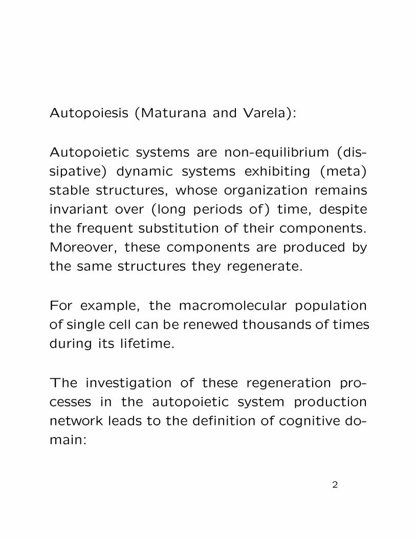
Autopoiesis (Maturana and Varela):

Autopoietic systems are non-equilibrium (dis-

sipative) dynamic systems exhibiting (meta)

stable structures, whose organization remains

invariant over (long periods of) time, despite

the frequent substitution of their components.

Moreover, these components are produced by

the same structures they regenerate.

For example, the macromolecular population

of single cell can be renewed thousands of times

during its lifetime.

The investigation of these regeneration pro-

cesses in the autopoietic system production

network leads to the definition of cognitive do-

main:

2

Maturana and Varela (1980):

“Our aim was to propose the characterizationof living systems that explains the generationof all the phenomena proper to them. Wehave done this by pointing at Autopoiesis inthe physical space as a necessary and sufficientcondition for a system to be a living one.”

“An autopoietic system is organized (definedas a unity) as a network of processes of produc-tion (transformation and destruction) of com-ponents that produces the components which:

(i) through their interactions and transforma-tions continuously regenerate and realize thenetwork of processes (relations) that producedthem; and

(ii) constitute it (the machine) as a concreteunity in the space in which they (the compo-nents) exist by specifying the topological do-main of its realization as such a network.”

3

Cognitive Domain (Maturana and Varela):

... Thus the circular organization implies the

prediction that an interaction that took place

once will take place again...

Every interaction is a particular interaction,

but every prediction is a prediction of a class

of interactions that is defined by those fea-

tures of its elements that will allow the living

system to retain its circular organization after

the interaction, and thus, to interact again.

This makes living systems inferential systems,

and their domain of interactions a cognitive

domain.”

4

Objects as Tokens for Eigen-Solutions

(von Foerster):

“The meaning of recursion is to run through

one’s own path again. One of its results is

that under certain conditions there exist in-

deed solutions which, when reentered into the

formalism, produce again the same solution.

These are called “eigen-values”, “eigen- func-

tions”, “eigen-behaviors”, etc., depending on

which domain this formation is applied.”

“Objects are tokens for eigen-behaviors.

Tokens stand for something else.

In exchange for money (a token itself for gold),

...tokens are used to gain admittance to the

subway or to play pinball machines.

In the cognitive realm, objects are the token

names we give to our eigen-behavior.

This is the constructivist’s insight into what

takes place when we talk about our experience

with objects.”

5

Eigen-Solution Ontology(von Foerster):

“Eigenvalues have been found onto-logically to be discrete, stable, separa-ble and composable, while ontogenet-ically to arise as equilibria that deter-mine themselves through circular pro-cesses. Ontologically, Eigenvalues andobjects, and likewise, ontogenetically,stable behavior and the manifestationof a subject’s “grasp” of an object can-not be distinguished.”

6

a- Discrete (or sharp):

“There is an additional point I want to make,

an important point. Out of an infinite contin-

uum of possibilities, recursive operations carve

out a precise set of discrete solutions. Eigen-

behavior generates discrete, identifiable enti-

ties. Producing discreteness out of infinite va-

riety has incredibly important consequences. It

permits us to begin naming things. Language

is the possibility of carving out of an infinite

number of possible experiences those experi-

ences which allow stable interactions of your-

self with yourself.”

It is important to realize that, in the sequel,

the term “discrete”, used by von Foerster to

qualify eigen-solutions in general, should be

replaced, depending on the specific context,

by terms such as lower-dimensional, precise,

sharp, singular, etc.

7

b- Equilibria (or stable):

A stable eigen-solution of the operator Op( ),

defined by the fixed-point or invariance equa-

tion, xinv = Op(xinv), can be found (built or

computed) as the limit, x∞, of the sequence

{xn}, as n →∞, by the recursive application of

the operator, xn+1 = Op(xn).

Under appropriate conditions (such as within a

domain of attraction, for instance) the process

convergence and its limit eigen-solution do not

depend on the starting point, x0.

We want to show, for statistical analysis in a

scientific context, how the property of sharp-

ness indicates that many, and perhaps some

of the most relevant, scientific hypotheses are

sharp, and how the property of stability, indi-

cates that considering these hypotheses is nat-

ural and reasonable.8

Coupling (Maturana and Varela):

“Whenever the conduct of two or more units is

such that there is a domain in which the con-

duct of each one is a function of the conduct

of the others, it is said that they are coupled

in that domain.”

“An autopoietic system whose autopoiesis en-

tails the autopoiesis of the coupled autopoietic

units which realize it, is an autopoietic system

of higher order.”

A typical example of a hierarchical system is

a Beehive, a third order autopoietic system,

formed by the coupling of individual Bees, the

second order systems, which, in turn, are formed

by the coupling of individual Cells, the first or-

der systems.

9

Social Systems (Luhmann):

“Social systems use communication as their

particular mode of autopoietic (re)production.

Their elements are communications that are

recursively produced and reproduced by a net-

work of communications that are not living

units, they are not conscious units, they are

not actions. Their unity requires a synthesis

of three selections, namely information, utter-

ance and understanding (including misunder-

standing).”

10

Differentiation (Luhmann):

Societys’ strategy to deal with increasing com-

plexity is the same one observed in most bio-

logical organisms, namely, differentiation.

Biological organisms differentiate in specialized

systems, such as organs and tissues of a pluri-

cellular life form (non-autopoietic or allopoietic

systems), or specialized individuals in an insect

colony (autopoietic system).

In fact, societies and organisms can be charac-

terized by the way in which they differenciate

into systems.

Modern societies are characterized by a verti-

cal differenciation into autopoietic functional

systems, where each system is characterized

by its code, program and (generalized) media.

11

-The code gives a bipolar reference to the sys-tem, of what is positive, accepted, favored orvalid, versus what is negative, rejected, disfa-vored or invalid.-The program gives a specific context wherethe code is applied.-The (generalized) media is the space in whichthe system operates.

Standard examples of social systems are:

Science: code: true/false; program: scientifictheory; media: journals, proceedings.

Judicial: code: legal/illegal; program: lawsand regulations; media: legal documents.

Religion: code: good/evil; program: sacredand hermeneutic texts; media: study, prayerand good deeds.

Economy: code: property / lack thereof;program: economic scenario, pricing method;media: money, assets.

12

Dedifferentiation (Luhmann):

Dedifferentiation (Entdifferenzierung) is thedegradation of the system’s internal coherence,through adulteration, disruption, or dissolutionof its own autopoietic relations.One form of dedifferentiation (in either biolog-ical or social systems) is the system’s penetra-tion by external agents who try to use system’sresources in a way that is not compatible withthe system’s autonomy.

“Autopoieticists claim that the smooth func-tioning of modern societies depends criticallyon maintaining the operational autonomy ofeach and every one of its functional (sub) sys-tems.”

Each system may be aware of events in othersystems (be cognitively open) but is requiredto maintain its differentiation (be operationallyclosed).

13

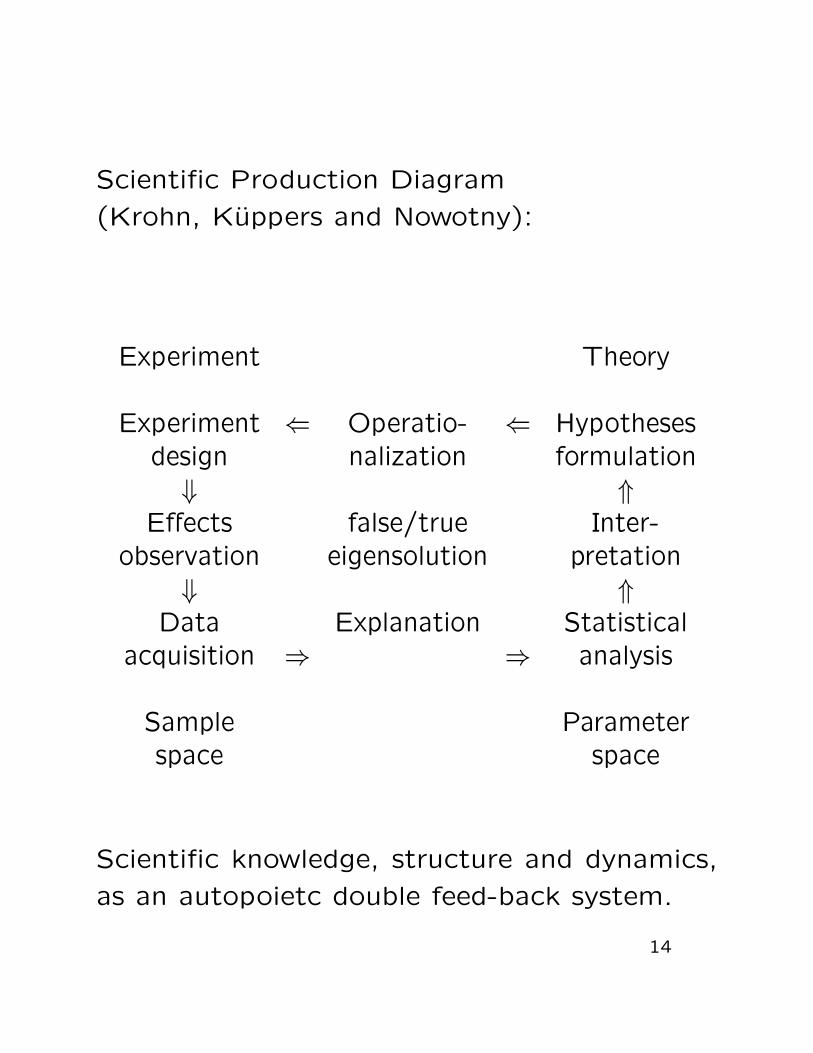
Scientific Production Diagram

(Krohn, Kuppers and Nowotny):

Experiment Theory

Experiment ⇐ Operatio- ⇐ Hypothesesdesign nalization formulation⇓ ⇑

Effects false/true Inter-observation eigensolution pretation

⇓ ⇑Data Explanation Statistical

acquisition ⇒ ⇒ analysis

Sample Parameterspace space

Scientific knowledge, structure and dynamics,

as an autopoietc double feed-back system.

14

Predictive Probabilities:

(stated in the sample space)

- At the Experiment side of the diagram, the

task of statistics is to make probabilistic state-

ments about the occurrence of pertinent events,

i.e. describe probabilistic distributions for what,

where, when or which events can occur.

Statistical Support of Hypotheses:

(stated in the parameter space)

- At the Theory side of the diagram, the role of

statistics is to measure the statistical support

of (sharp) hypotheses, i.e. to measure, quan-

titatively, the hypothesis plausibility or possi-

bility in the theoretical framework they were

formulated, given the observed data.

15

Probabilistic Statements:

Frequentist probabilistic statements are made

exclusively on the basis of the frequency of oc-

currence of an event in a (potentially) infinite

sequence of observations generated by a ran-

dom variable.

Epistemic probabilistic statements are made

on the basis of the epistemic status (degree of

belief, likelihood, truthfulness, validity) of an

event from the possible (actual or potential)

outcomes generated by a random variable.

Bayesian probabilistic statements are epistemic

probabilistic statements generated by the (in

practice, always finite) recursive use of Bayes

formula:

pn(θ) ∝ pn−1(θ)p(xn|θ) .

16

Frequentist (Classical) Statistics,

dogmatically demands that all probabilistic state-

ments be frequentist. Therefore, any direct

probabilistic statement on the parameter space

is categorically forbidden.

Scientific hypotheses are epistemic statements

about the parameters of a statistical model.

Hence, frequentist statistics can not make any

direct statement about the statistical signifi-

cance (truthfulness) of hypotheses.

Strictly speaking it can only make statements

at the Experiment side of the diagram.

The frequentist way of dealing with questions

on Theory side of the diagram, is to embed

them some how into the Experiment side.

A p-value (of the data bank, not of the hy-

pothesis) is the probability of getting a sample

that is more extreme (incompatible with H)

than the one we got.

17

Bayesian statistics,

allows probabilistic statements on the param-

eter space, and also, of course, in the sample

space. Thus it seems that Bayesian statistics

is the right tool for the job, and so it is!

Nevertheless, we must first examine the role

played by DecTh (decision theory) in the foun-

dations of orthodox Bayesian statistics (strat-

ified in two layers):

- First layer: DecTh provides a coherence sys-

tem for the use of probability statements, see

Finetti (1974, 1981). FBST use of probability

theory is fully compatible with DecTh in this

layer, Madruga (2001).

- Second layer: DecTh provides an epistemo-

logical framework for the interpretation of sta-

tistical procedures:

18

Betting on Theories (Savage):

“Gambling problems ... seem to embrace the

whole of theoretical statistics according to the

decision-theoretic view of the subject.

... the gambler in this problem is a person who

must act in one of two ways (two guesses),...

appropriate under (H0) or its negation (H1).

...The unacceptability of extreme (sharp) null

hypotheses is perfectly well known; it is closely

related to the often heard maxim that science

disproves, but never proves, hypotheses.

... The role of extreme (sharp) hypotheses in

science ... seems to be important but obscure.

...I cannot give a very satisfactory analysis...

nor say clearly how it is related to testing as

defined in (DecTh) theoretical discussions.”

19

In the DecTh framework we speak about the

betting odds for “getting the hypothesis on a

gamble taking place in the parameter space”.

But sharp hypotheses are zero (Lebesgue) mea-

sure sets, so our betting odds must be null, i.e.

sharp hypotheses are (almost) surely false.

If we accept the ConsTh view that an impor-

tant class of hypotheses concern the identifi-

cation of eigen-solutions, and that those are

ontologically sharp, we have a paradox!

20

The Full Bayesian Significance Test, FBST,

was specially designed to give an evidence value

supporting a sharp hypothesis, H. This sup-

port function, Ev(H, pn), is based on the pos-

terior pobability measure of a set called the

tangential set T (H, pn), which is a non zero

measure set (so no null probability paradoxes).

Furthermore Ev( ) has many necessary or de-

sirable properties for a statistical support func-

tion, such as:

1- Give an intuitive and simple measure of sig-

nificance for the (null) hypothesis, ideally, a

probability defined directly in the original or

natural parameter space.

2- Be able to provide a consistent test for a

given sharp hypothesis.

21

3- Have an intrinsically geometric definition,

independent of any non-geometric aspect, like

the particular parameterization of the hypoth-

esis (manifold) being tested, or the particular

coordinate system chosen for the parameter

space, i.e., be an invariant procedure.

4- Require no ad hoc artifice like assigning a

positive prior probability to zero measure sets,

or setting an arbitrary initial belief ratio be-

tween hypotheses.

5- Give a possibilistic support structure for hy-

potheses, and so comply with the Onus Probandi

juridical principle (In Dubito Pro Reo rule), i.e.

consider in the “most favorable way” the claim

stated by the hypothesis.

22

6- Obey the likelihood principle : The infor-

mation gathered from observations should be

represented (only) by the likelihood function.

7- Allow the incorporation of previous experi-

ence or expert’s opinion via “subjective” prior

distributions.

8- Be an exact procedure, i.e., make no use of

“large sample” asymptotic approximations.

9- Give a measure of significance that is smooth,

i.e. continuous and differentiable, on the hy-

pothesis parameters and sample statistics, un-

der appropriate regularity conditions.

23

Semantic Degradation:

Hopefully it’s now clear that several technicaldifficulties of testing (sharp) hypotheses in thetraditional statistical paradigms are symptomsof problems with much deeper roots.Regarding the abuse of (pseudo) economicalanalyses, see Luhmann (1989):

“In this sense, it is meaningless to speak of“non-economic” costs. This is only a metaphor-ical way of speaking that transfers the speci-ficity of the economic mode of thinking indis-criminately to other social systems.”

Once the forces pushing for systemic degrada-tion are exposed, we hope one can understandour (aphoristic, double) plea for sanity:

Preserve systemic autopoiesis and semantic in-tegrity, for de-differentiation is in-sanity itself.

Chose the right tool for each job: “If you onlyhave a hammer, everything looks like a nail”.

24

Competing Sharp Hypotheses (Good):

Never test a single sharp hypothesis, an unfairfaith of the poor sharp hypothesis standing allalone against everything else in the world.Instead, always confront a sharp hypothesiswith a competing sharp hypotheses, a fair game.

“...If by the truth of Newtonian mechanics wemean... approximately true, we could obtainstrong evidence that it is true; but if we mean...exactly true, then it has already been refuted.”

“...I think that the initial probability is posi-tive for every self-consistent scientific theory...since the number of statable theories is at mostcountably infinite (enumerable).”

“...It is difficult to decide... numerical proba-bilities, but it is not so difficult to judge theratio of initial probabilities of two theories bycomparing their complexities. ...(that’s) whyhistory of science is scientificaly important.”

25

The competing sharp hypotheses argument

does not contradict the ConsTh epistemolog-

ical framework, and it may be appropriate in

certain circumstances. It may also mitigate

or partially remediate the paradoxes of testing

sharp hypotheses in the traditional frequentist

or orthodox Bayesian settings (Bayes factors,

Jeffreys’ tests). However, we do not believe

that having it is neither a necessary condition

for good science practice, nor an accurate de-

scription of science history.

Quickly examine the very first major incident

in the tumultuous debacle of Newtonian me-

chanics (just to stay with Good’s example).

This incident was Michelson’s experiment on

the effect of “etherial wind” over the speed of

light. Michelson found no such effect, i.e. he

found the speed of light to be constant, in-

variant with the relative speed of the observer

(with no competing theory at that time).

26

Noether’s Theorem:

For every continuous symmetry in a physical

theory, there must exist an invariant quantity

or conservation law:

Galileo’s group ⇒ Newtonian mechanics ⇒Newtonian objects (ex. momentum, enery).

Lorentz’ goup ⇒ Einstein’s relativity ⇒Relativistic objects (ex. energy-momentum).

Conserv. laws are “ideal” sharp hypotheses.

Careful with competing theories historical anal-

yses “ex post facto” or “post mortem”.

Complex experiments require careful error and

fluctuation analysis, and realistic (complex) sta-

tistical models. All statistically significant in-

fluences should be incorporated into the model.

27

De Finetti type Theorems,

given an invariance transformation group

(like permutability, spherical symmetry, etc.),

provide invariant distributions, that can in turn

provide prototypical sharp hypotheses in many

application areas.

Physics has its own heavy apparatus to deal

with the all important issues of invariance and

symmetry.

Statistics, via de Finetti theorems, can provide

such an apparatus for other areas, even in sit-

uations that are not naturally embedded in a

heavy mathematical formalism.

28

Compositionality

(von Foerster):

“...Eigenvalues have been found ontologically

to be ...separable and composable...

(Luhmann, evolution of science):

“...something that idealization, mathematiza-

tion, abstraction, etc. do not describe ade-

quately. It concerns the increase in the ca-

pacity of decomposition and recombination, a

new formulation of knowledge as the product

of analysis and synthesis. ...(that) uncovers an

enormous potential for recombination.”

29

FBST - Full Bayesian Significance Test

Bayesian paradigm: the posterior density, pn(θ),

is proportional to the product of the likelihood

and a prior density,

pn(θ) ∝ L(θ |x) p0(θ).

(Null) Hypothesis: H : θ ∈ ΘH ,

ΘH = {θ ∈ Θ | g(θ) ≤ 0 ∧ h(θ) = 0}

Precise hypothesis: dim(ΘH) < dim(Θ).

Reference density, r(θ), interpreted as a rep-

resentation of no information in the param-

eter space, or the limit prior for no obser-

vations, or the neutral ground state for the

Bayesian operation. Standard (possibly im-

proper) uninformative references include the

uniform and maximum entropy densities, see

Dugdale (1996) and Kapur (1989)

30

FBST evidence value supporting and against

the hypothesis H, Ev(H) and Ev(H),

s(θ) = pn (θ) /r (θ) ,

s = s(θ) = supθ∈Θ s(θ) ,

s∗ = s(θ∗) = supθ∈H s(θ) ,

W (v) =∫T

pn (θ) dθ , W = 1−W (v) ,

T = {θ ∈ Θ | s(θ) ≤ s∗} , T = Θ− T ,

Ev(H) = W (s∗) , Ev(H) = W (s∗) = 1−Ev(H) .

s(θ) is the posterior surprise relative to r(θ).

The tangential set T is a HRSS.

(Highest Relative Surprise Set)

W (v) is the cumulative surprise distribution.

Ev(H) is invariant under reparameterizations.

If r ∝ 1 then s(θ) = pn(θ) and T is a HPDS.

31

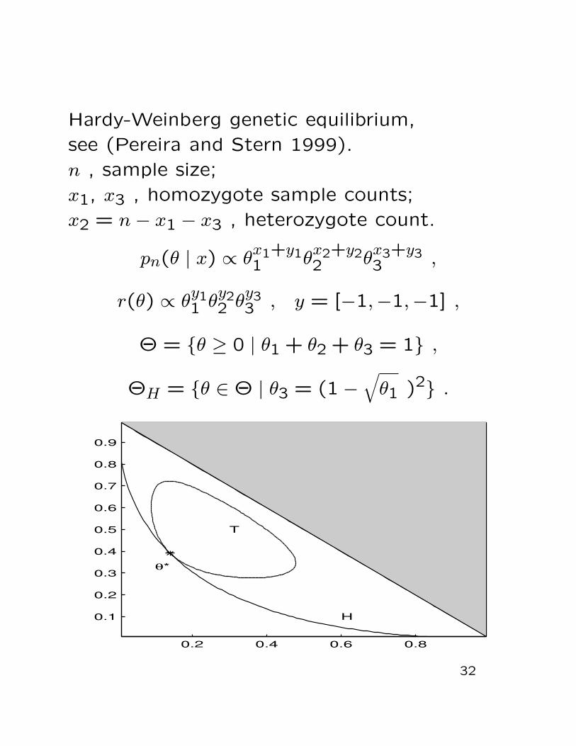
Hardy-Weinberg genetic equilibrium,

see (Pereira and Stern 1999).

n , sample size;

x1, x3 , homozygote sample counts;

x2 = n− x1 − x3 , heterozygote count.

pn(θ | x) ∝ θx1+y11 θ

x2+y22 θ

x3+y33 ,

r(θ) ∝ θy11 θ

y22 θ

y33 , y = [−1,−1,−1] ,

Θ = {θ ≥ 0 | θ1 + θ2 + θ3 = 1} ,

ΘH = {θ ∈ Θ | θ3 = (1−√

θ1 )2} .

0.2 0.4 0.6 0.8

0.1

0.2

0.3

0.4

0.5

0.6

0.7

0.8

0.9

H

T

θ*

32

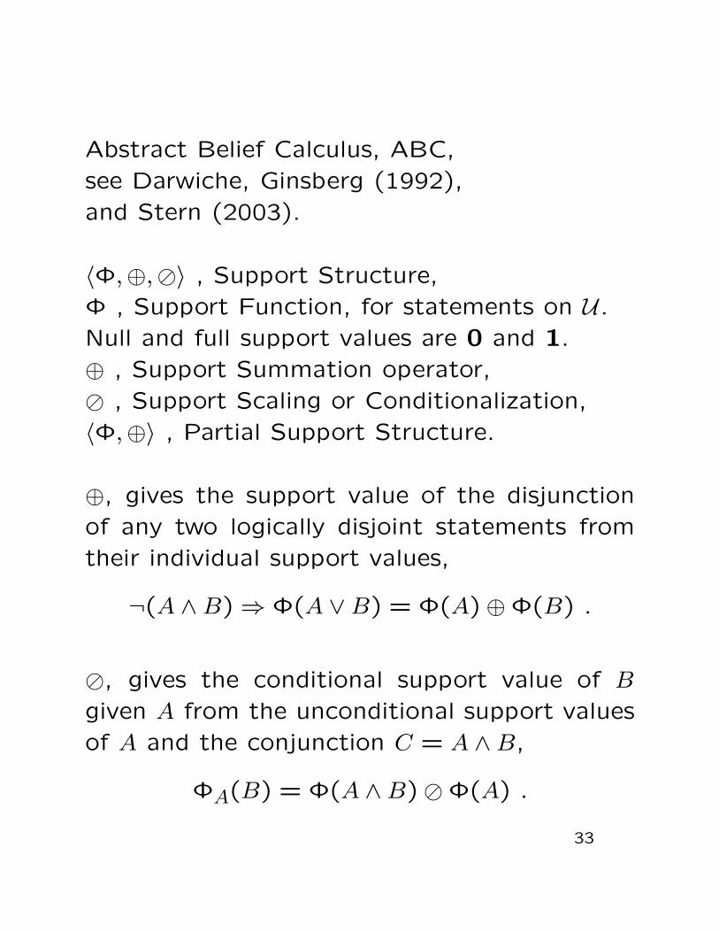
Abstract Belief Calculus, ABC,

see Darwiche, Ginsberg (1992),

and Stern (2003).

〈Φ,⊕,�〉 , Support Structure,

Φ , Support Function, for statements on U.

Null and full support values are 0 and 1.

⊕ , Support Summation operator,

� , Support Scaling or Conditionalization,

〈Φ,⊕〉 , Partial Support Structure.

⊕, gives the support value of the disjunction

of any two logically disjoint statements from

their individual support values,

¬(A ∧B) ⇒ Φ(A ∨B) = Φ(A)⊕Φ(B) .

�, gives the conditional support value of B

given A from the unconditional support values

of A and the conjunction C = A ∧B,

ΦA(B) = Φ(A ∧B)�Φ(A) .

33

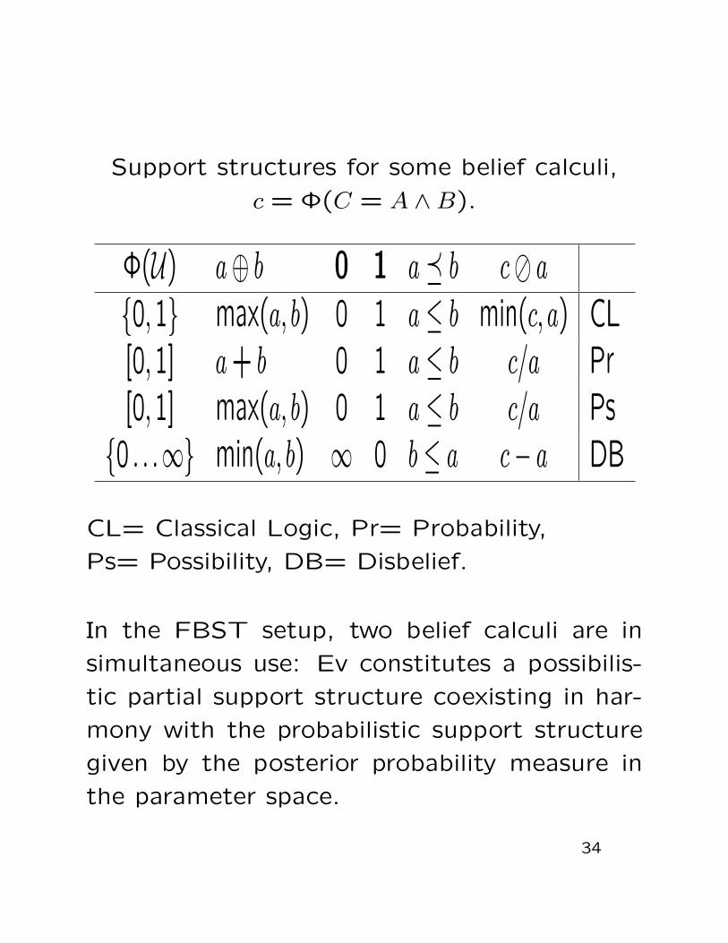
Support structures for some belief calculi,

c = Φ(C = A ∧B).

Φ(U) a⊕ b 0 1 a � b c� a{0,1} max(a, b) 0 1 a ≤ b min(c, a) CL[0,1] a + b 0 1 a ≤ b c/a Pr[0,1] max(a, b) 0 1 a ≤ b c/a Ps

{0 . . .∞} min(a, b) ∞ 0 b ≤ a c− a DB

CL= Classical Logic, Pr= Probability,

Ps= Possibility, DB= Disbelief.

In the FBST setup, two belief calculi are in

simultaneous use: Ev constitutes a possibilis-

tic partial support structure coexisting in har-

mony with the probabilistic support structure

given by the posterior probability measure in

the parameter space.

34

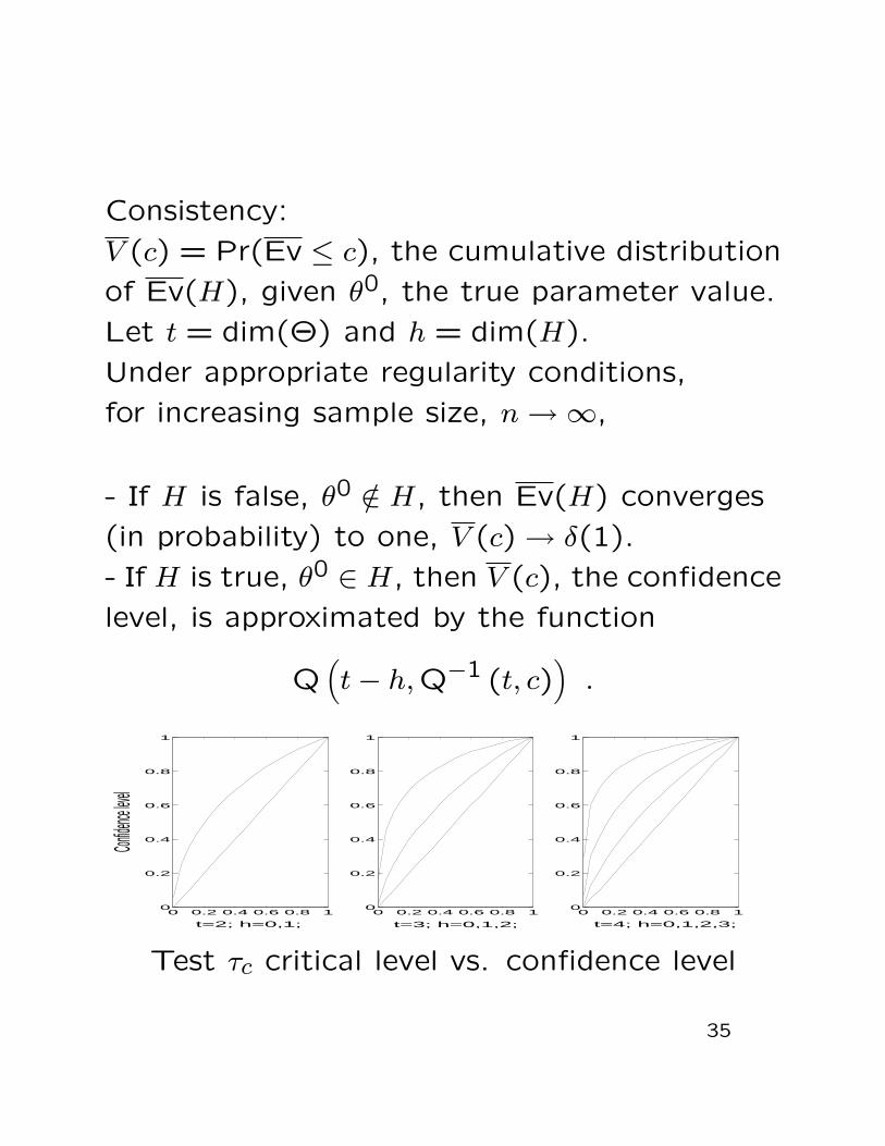
Consistency:

V (c) = Pr(Ev ≤ c), the cumulative distribution

of Ev(H), given θ0, the true parameter value.

Let t = dim(Θ) and h = dim(H).

Under appropriate regularity conditions,

for increasing sample size, n →∞,

- If H is false, θ0 /∈ H, then Ev(H) converges

(in probability) to one, V (c) → δ(1).

- If H is true, θ0 ∈ H, then V (c), the confidence

level, is approximated by the function

Q(t− h,Q−1 (t, c)

).

0 0.2 0.4 0.6 0.8 10

0.2

0.4

0.6

0.8

1

Confide

nce leve

l

t=2; h=0,1;

0 0.2 0.4 0.6 0.8 10

0.2

0.4

0.6

0.8

1

t=3; h=0,1,2;

0 0.2 0.4 0.6 0.8 10

0.2

0.4

0.6

0.8

1

t=4; h=0,1,2,3;

Test τc critical level vs. confidence level

35

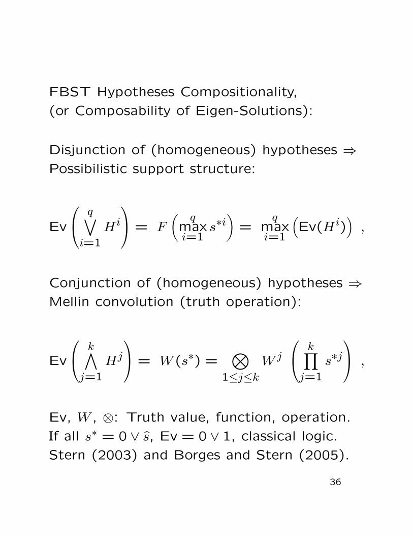
FBST Hypotheses Compositionality,

(or Composability of Eigen-Solutions):

Disjunction of (homogeneous) hypotheses ⇒Possibilistic support structure:

Ev

q∨i=1

Hi

= F

(q

maxi=1

s∗i)

=q

maxi=1

(Ev(Hi)

),

Conjunction of (homogeneous) hypotheses ⇒Mellin convolution (truth operation):

Ev

k∧j=1

Hj

= W (s∗) =⊗

1≤j≤k

W j

k∏j=1

s∗j ,

Ev, W , ⊗: Truth value, function, operation.

If all s∗ = 0 ∨ s, Ev = 0 ∨ 1, classical logic.

Stern (2003) and Borges and Stern (2005).

36