Previous Version: May, 17 2001 This version: July 7, 2001

Cognition and Wealth:

The Importance of Probabilistic Thinking

Lee A. Lillard Michigan Retirement Research Center (MRRC), University of Michigan

and Robert J. Willis

Health and Retirement Study (HRS), University of Michigan

The research herein was performed pursuant to a grant from the U.S. Social Security Administration (SSA) to the Michigan Retirement Research Center (MRRC project number UM 00-04). The opinions and conclusions are solely those of the authors and should not be construed as representing the opinions or policy of SSA or any agency of the Federal Government of the MRRC. Additional support was received by the second author from NIA grant P01 AG10179. Data from the Health and Retirement Study used in this paper were funded by the National Institute of Aging, grant number AG09740, with additional support from SSA. We are grateful for research assistance by Jody Schimmel, Helena Stolyarova and, especially, to Gabor Kezdi who make a number of important suggestions and contributions. We are also grateful for comments on earlier versions of this paper by workshop participants at the University of Michigan, the University of Bergen, Northwestern University, TMR Conference-Paris, University of Chicago, Washington University, and the University of Maryland, the NBER Workshop on Uncertainty, Conference of Retirement Research Consortium and discussions with Gary Becker, Eric French, Jim Heckman, Chuck Manski, Olivia Mitchell, Sherwin Rosen, Mark Rosenzweig, Matthew Shapiro, Jim Smith, Yoram Weiss, and Doug Wolf.

Cognition and Wealth: The Importance of Probabilistic Thinking

Lee A. Lillard* and Robert J. Willis** University of Michigan

Abstract This paper utilizes a large set of subjective probability questions from the Health and Retirement Survey to construct an index measuring the precision of probabilistic beliefs (PPB) and relates this index to household choices about the riskiness of their portfolios and the rate of growth of their net worth. A theory of uncertainty aversion based on repeated sampling is proposed that resolves the Ellsberg Paradox within a conventional expected utility model. In this theory, uncertainty aversion is implied by risk aversion. This theory is then used to propose a link between an individual’s degree of uncertainty and his propensity to give “focal” answers of “0”, “50_50” or “100” or “exact” answers to survey questions and the validity of this interpretation is tested empirically. Finally, an index of the precision of probabilistic thinking is constructed by calculating the fraction of probability questions to which each HRS respondent gives a non-focal answer. This index is shown to have a statistically and economically significant positive effect on the fraction of risky assets in household portfolios and on the rate of growth of these assets longitudinally. These results suggest that there is systematic variation in the competence of individuals to manage investment accounts that should be considered in designing policies to create individual retirement accounts in the Social Security system. *Lee Lillard died on December 2, 2000. **rjwillis@umich.edu

1

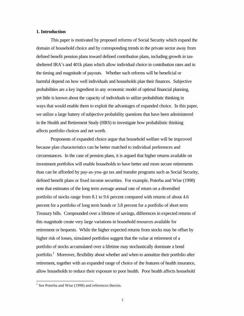
1. Introduction

This paper is motivated by proposed reforms of Social Security which expand the

domain of household choice and by corresponding trends in the private sector away from

defined benefit pension plans toward defined contribution plans, including growth in tax-

sheltered IRA’s and 401k plans which allow individual choice in contribution rates and in

the timing and magnitude of payouts. Whether such reforms will be beneficial or

harmful depend on how well individuals and households plan their finances. Subjective

probabilities are a key ingredient in any economic model of optimal financial planning,

yet little is known about the capacity of individuals to utilize probabilistic thinking in

ways that would enable them to exploit the advantages of expanded choice. In this paper,

we utilize a large battery of subjective probability questions that have been administered

in the Health and Retirement Study (HRS) to investigate how probabilistic thinking

affects portfolio choices and net worth.

Proponents of expanded choice argue that household welfare will be improved

because plan characteristics can be better matched to individual preferences and

circumstances. In the case of pension plans, it is argued that higher returns available on

investment portfolios will enable households to have better and more secure retirements

than can be afforded by pay-as-you–go tax and transfer programs such as Social Security,

defined benefit plans or fixed income securities. For example, Poterba and Wise (1998)

note that estimates of the long term average annual rate of return on a diversified

portfolio of stocks range from 8.1 to 9.6 percent compared with returns of about 4.6

percent for a portfolio of long term bonds or 3.8 percent for a portfolio of short term

Treasury bills. Compounded over a lifetime of savings, differences in expected returns of

this magnitude create very large variations in household resources available for

retirement or bequests. While the higher expected returns from stocks may be offset by

higher risk of losses, simulated portfolios suggest that the value at retirement of a

portfolio of stocks accumulated over a lifetime may stochastically dominate a bond

portfolio.1 Moreover, flexibility about whether and when to annuitize their portfolio after

retirement, together with an expanded range of choice of the features of health insurance,

allow households to reduce their exposure to poor health. Poor health affects household

1 See Poterba and Wise (1998) and references therein.

2

income and wealth primarily through medical expenditures and (mostly uninsurable)

losses in labor income (Smith 1999b). Even insurance against inflation risk, a traditional

advantage of Social Security benefits, is now attainable for households who choose to

hold indexed Treasury bonds.

Although expanded choice offers many important potential benefits to

households, critics argue that large segments of the population will fail to make choices

that exploit these potential benefits and, consequently, the expansion of choice will

expose these segments of the population to greater risks of poverty and exacerbate the

already very large inequalities in wealth among older households. Some of the reasons

given for these worries fit within the conventional life cycle model of expected utility

maximization. For example, in the presence of incomplete insurance and annuity markets,

risk aversion might lead low income households to choose less risky portfolios with

lower expected returns than higher income households. There may also be variation in

taste parameters, such as time preference, such that persons with high rates of time

preference save at low rates (and also choose lower investments in human capital and less

healthy lifestyles), which leave them with poor health and few resources in old age.

Those who emphasize “equality of opportunity” may view such outcomes as an

acceptable consequence of the exercise of free choice. Those who value “equality of

outcomes” stress the value of placing constraints on choice ex ante, both to protect others

from the bad consequence of their actions and to protect themselves from higher taxes to

fund redistributional programs needed to offset these consequences.

This paper utilizes a large battery of subjective probability questions that have

been administered to a sample of over 20,000 individuals in the 1998 wave and earlier

waves of the Health and Retirement Study (HRS) and its companion study, Asset and

Health Dynamics of the Oldest Old (AHEAD). Our goal is to develop a measure of

competence in probabilistic thinking which is based on the degree to which an

individual’s probabilistic beliefs are precise or imprecise and examines the empirical

relationship between this measure and measures of asset accumulation and portfolio

composition. We provide a theoretical justification for our approach using a simple

model in which people with imprecise probability beliefs behave in a more risk averse

manner than those with more precise beliefs. Our model represents a possible resolution

3

of the “Ellsberg Paradox” (Ellsberg 1961), which alleges that individuals display

“uncertainty aversion.” Unlike most models of uncertainty aversion, our model is

compatible with rationality as defined by the axioms underlying the Ramsey-Savage

theory of personal probabilities (Ramsey 1926, Savage 1954), Baysesian statistical theory

and the Von Neuman-Morgenstern subjective expected utility (SEU) model .2 In addition

to providing a link between probabilistic thinking and uncertainty aversion, the model

also provides a framework which could be used to study how individuals may acquire

more precise information about probabilities, how they may increase the precision of

their beliefs through experimentation, and how information acquisition is related to

preference parameters such as risk aversion and time preference. These further

implications are not pursued in this paper.

The plan of the paper is as follows. Section 2 provides a discussion of the

subjective probability questions in the HRS and some background about the elicitation of

data on expectations in a survey context. The distribution of responses to these

probability questions suggests that there may be considerable heterogeneity among

respondents in the precision their probability beliefs and/or their competence in

probabilistic thinking. In Section 3, we discuss the idea of uncertainty aversion in the

context of the Ellsberg paradox. In Section 4 we develop a rational model of uncertainty

aversion. In Section 5, we consider how survey responses to probability questions are

related to the precision of probability beliefs. Section 6 presents an econometric analysis

relating measures of imprecise probability beliefs to the share of risky assets in household

portfolios and to the growth rate of household assets. A summary and conclusions are

presented in Section 7.

2 After formulating our model, we discovered that Scheeweiss (1999) independently proposed essentially the same resolution of the Ellsberg Paradox. He does not, however, discuss the implications of the model for learning or apply it empirically.

2. Subjective Probability Questions in the HRS

This paper makes use of a unique body of data on large number of subjective

probability questions asked to respondents in several longitudinal waves of the Health

and Retirement Study.3 In this paper, we analyze questions asked in the 1998 wave which

surveyed a national probability sample of over 22,000 respondents representing the U.S.

population over age 50, as well as questions asked to subsets of these persons in other

waves.4 These probability questions cover a wide range of topics ranging from personal

life expectancy and date of retirement to beliefs about the rate of inflation, future Social

Security policy and other macro-level variables.

The format of the probability questions is presented in Table 1. There is an

introduction which states that the respondent will be asked some questions about how

likely they think various events might be. For each question, the respondent is told to

give a number between 0 and 100 where “0” means “no chance at all” and “100” means

the event is absolutely sure to happen. In several waves of the survey, a “warm up”

question is asked about the chance that tomorrow will be sunny,5 followed by a list of

questions on a variety of topics. Several examples of probability questions are given in

Table 1, classified by whether they are about general events (e.g., social security

generosity or rate of inflation), events with personal knowledge (e.g., survival to age 75,

income will keep up with inflation) or events subject to personal control (e.g., leaving an

3 See Dominitz and Manski (1999) for a discussion of the history of methods of eliciting expectations data in surveys. 4 The initial HRS sample, consisting of 12,654 persons born in 1931-41, was first surveyed in 1992 when respondents were 51-61 years of age and has been resurveyed in 1994, 1996 and 1998. The AHEAD survey, consisting of 8,221 persons born before 1924, were first surveyed in 1993 when they were 70 years of age and up and were followed up in 1995. Beginning with 1998, the AHEAD survey of persons born before 1924 has been integrated into the HRS which also incorporated a new cohort born in 1924-30 who were entering their 70’s and another new cohort born in 1942-47 who were entering their 50’s. Thus, the 1998 wave of the HRS represents the entire U.S. population over age 50. See Juster and Suzman (1995), Soldo, et. al. (1997) and Willis (1999) for more detailed descriptions of the HRS and AHEAD studies. 5 Basset and Lumsdaine (1999a) have used this question to investigate whether some individuals are persistently “optimistic” or “pessimistic”. They find that persons who give high probabilities that the

5

inheritance or working at age 62). In HRS-1998, there were seventeen probability

questions. Some questions were asked to a subset of respondents (e.g., the probability of

working at age 62 was only asked of those less than age 62). Others contain additional

sub-questions, depending on the answer (e.g., if the probability of leaving an inheritance

is larger than zero, the respondent is asked about the probability of leaving inheritances

larger than $10,000 and, subject to that probability being positive, the probability of

leaving more than $100,000).

Analysis of the subjective probability questions has demonstrated that they

contain considerable useful information. For example, on average, subjective

probabilities of life expectancy match life tables surprisingly well and co-vary with

variables such as smoking, drinking, health conditions or education in ways that would be

expected from studies of actual mortality (Hurd and McGarry, 1995). As another

example, Smith (1999a) finds that average values of expected bequest probabilities

behave in sensible ways and appear to provide genuine information about behavior.

Although the subjective probability responses in HRS seem to “work well” when

averaged across respondents, individual responses appear to contain considerable noise

and are often heaped on “focal values” of “0”, “50” and “100”.6 The degree of heaping is

apparent in Figure 2 which presents histograms of the answers to the six probability

questions listed in Table 1. A comprehensive tabulation of focal answers to all

probability questions in HRS-1998 is presented in Table 2. On average, only 5% of

respondents refused to answer the probability questions. However, 52% of questions

were heaped on either “0” or “100” and an additional 15% were heaped on “50”.

Probabilities and probabilistic thinking are crucial ingredients of economic

models of decision making about asset accumulation and portfolio choice. In this paper,

we hypothesize that a persistent tendency to give focal answers to probability questions

indicates that a respondent has imprecise beliefs about the true value of a probability.

weather will be sunny tomorrow tend to give higher probabilities of “good” outcomes on other topics. This question was omitted from HRS-1998, but has been put back into HRS-2000 which is currently in the field. 6 Several researchers who have analyzed the HRS data emphasize the large number of focal answers and show that the likelihood of such answers is correlated with education and cognitive measures (see, especially, Hurd, McFadden and Gan (1998)). In addition, Bassett and Lumsdaine (1999b) find other evidence of noise and unobserved hetereogeneity in answers to these questions.

6

Further, we hypothesize that imprecise beliefs about probabilities will lead an individual

to make conservative financial choices which yield lower wealth and lower rates of

wealth accumulation than otherwise similar individuals who have more precise

probability beliefs. In the next two sections, we explore a more formal theoretical

framework to understand why imprecise probabilistic thinking might lead to such a

relationship.

3. Probabilistic Thinking, Imprecise Beliefs and Uncertainty Aversion

Despite much criticism, subjective expected utility (SEU) theory remains the

dominant framework for economic models of decision making under uncertainty. (See

Starmer 2000, for a survey of alternatives to SEU theory). SEU theory assumes that

individuals decide on a given course of action by choosing that action which yields the

highest expected utility. For example, consider a decision between actions A and B by

individual i. The expected utilities associated with these actions are

(1) 1

aa a

ia ij ijj

EU p UΩ

=

= ∑ and 1

bb b

ib ij ijj

EU p UΩ

=

= ∑ ,

where there are aΩ discrete states of the world that might occur if action A is chosen and

bΩ states if B is chosen. aijp represents i’s beliefs about the probability that the jth state

of the world will occur and aijU is the utility i believes that he will receive in that state.

Similarly, bijp and b

ijU represent i’s beliefs about probabilities and utilities when B is

chosen. The individual’s choice of action is given by the decision rule

(2) ;a bi iChoose A if EU EU Otherwise Choose B> .

Taken literally, the SEU model presumes that individuals competently perform

some extremely demanding tasks before making any given decision. The individual must

be capable of imagining a large number of states of the world. Within each state, the

individual solves an optimization problem in which he maximizes his (possibly state-

dependent) utility subject to a set of constraints embodying his income and wealth

endowments, prices, state of health and all other data relevant to the optimization

problem. The outcome of this optimization yields the level of utility associated with that

state. Finally, the SEU model assumes that the individual has a coherent and well-

defined set of beliefs about the probabilities that each state will occur.

The latter assumption has been called into question at least since Frank Knight

(1921) introduced the distinction between “risk” and “uncertainty” where risk refers to a

situation in which a specific probability can be attached to a given outcome while

uncertainty refers to a situation in which a probability cannot be specified. For example,

examination of a symmetric coin may lead an individual to conclude that heads and tails

have equal probability, that there are no other possible outcomes and, consequently, that

8

the probability of heads is one half. Or, a person may have examined actuarial tables to

determine his probability of death this year. In contrast to these risks, uncertainty may

attach to questions in which there is neither a quantitative model of the random process,

such as the simple physical model of a coin described above, nor is there adequate data to

form a statistical estimate of the event from past frequencies of occurrence. Examples

range from mundane questions about the probability that a new start-up firm will be in

business in ten years or that a given marriage match will succeed to large questions such

as the probability of nuclear war or the probability that there is intelligent life elsewhere

in the universe.

The Ramsey-Savage theory of personal probability appeared to resolve this

problem by eliminating the distinction between risk and uncertainty within a Baysesian

framework in which individual preferences are assumed to fulfill certain axioms which

lead to rational, maximizing behavior (Savage, 1954). According to this theory, the

probabilities that enter into decision problems are subjective. Individuals are assumed to

have a set of prior beliefs about the probability of any given event given by the

distribution function, ( )f p . The probability of the event is simply given by the expected

value of this distribution, 1

0( )p pf p dp= ∫ . The probabilities entering the von Neumann-

Morgenstern expected utility function in (1) have this interpretation.

An influential challenge to this resolution was presented by Ellsberg (1961) in an

example that has come to be known as the “Ellsberg Paradox”. In one version of the

example, subjects are confronted with choices about betting on the outcome of draws

from two urns, Urn I and Urn II, each containing red and/or black balls. The subject

chooses which urn to play and the color of the ball to bet on. If a ball of the chosen color

is drawn, the subject wins $1; otherwise, he wins nothing. Urn I contains 50 red balls and

50 black balls. Urn II contains 100 red and black balls in unknown proportion.

When asked about which color they preferred to bet on, most subjects indicated

indifference regardless of which urn was under consideration. This suggests that subjects

believe that red and black are equiprobable in either urn. When asked which urn they

preferred to draw from, some subjects indicated indifference but a majority indicated a

preference for Urn I, explaining that they preferred the greater certainty about the

9

probability of drawing a ball of given color. The latter preference clearly violates the

Savage axioms.

The paradox that Ellsberg identified, and that subsequent experimental research

has verified, is that most people prefer a known risk to an uncertain one of equal expected

value. Ellsberg often found uncertainty aversion even in a decidedly non-random sample

of the founders of SEU theory. He reports that G. Debreu, R. Schlaiffer and P.

Samuelson do not violate the Savage axioms, while J. Marshak and N. Dalkey violate

them “cheerfully and even with gusto” and “others sadly but persistently, having looked

into their hearts, found conflicts with the axioms and decided, in Samuelson’s phrase, to

satisfy their preferences and let the axioms satisfy themselves.” (Ellsberg, pp. 655-56).

Interestingly, Ellsberg places Savage himself in the latter group. Among the violators, he

writes, “What is at issue might be called the ambiguity [italics in original] of this

information, a quality depending on the amount, type, reliability and `unanimity’ of

information, and giving rise to one’s degree of ‘confidence’ in an estimate of relative

likelihoods.” (Ellsberg, 1961, p. 657.)

Ellsberg and most of the subsequent literature react to this paradox by partially

giving up on the Savage axioms, instead suggesting non-rational preferences that allow

for “uncertainty aversion” in ambiguous situations. An example, is the maxmin expected

utility (MMEU) function originally proposed by Gilboa and Schmeidler (1989).

Intuitively, these preferences suggest that a decision maker who is uncertain about the

true probabilities governing the outcomes of his decision may focus special attention to

thinking about the consequences of the “worst case scenario” (among all “reasonable”

scenarios) and will make conservative choices according to a maxmin criterion.

4. A SEU Model of Uncertainty Aversion and Learning about Probabilities

In this section, we propose an alternative model of uncertainty aversion. Given

repeated sampling, individuals are fully rational in the sense that they behave in accord

with the SEU model, but they may have more or less precise beliefs about the “true

values” of the probabilities upon which their decisions are based.7 Ellsberg’s examples

all concern “one shot” bets on a single roll of a die or a single ball drawn from an urn.

Our model departs from the Ellsberg framework by assuming that most individuals

implicitly form their preferences among uncertain prospects in a context of real world

choices whose consequences determine repeated random outcomes. 8 Obvious examples

include the returns from investments in human or physical capital, the choice of a

marriage partner, or the returns from a stock held more than one period. In this model, it

is easy to show that uncertainty aversion is simply a consequence of risk aversion. In

addition, we show that if experimentation or other forms of learning such as job shopping

(Johnson 1978) are possible and decisions are reversible, then even risk averse people

may display uncertainty preference.

The basic idea of our model may be illustrated by continuing with Ellsberg’s urn

example, using a modified version in which two balls are drawn instead of one. Assume

that there are two urns, each containing red and black balls. By convention, assume that

there is a payoff of $1 each time a red ball is drawn from either urn and a zero payoff if a

7 An advantage of retaining the SEU model is that we can freely draw upon the entire body of conventional economic theory in our application whereas theories such as the MMEU theory mentioned above are not (yet) fully embedded in a broader economic model. We exploit this advantage later in this section when we show how utility aversion and learning may be related. 8 As noted earlier, Scheeweiss (1999) independently proposed essentially the same resolution of the Ellsberg Paradox.

11

black ball is chosen.9 After a ball is drawn from an urn and its color noted, it is returned

to the urn. Urn I contains a known number R red and B black balls. We assume that all

individuals agree that /( )p R R B= + is the probability of drawing a red ball from Urn I.

Urn II contains an uncertain number of red and black balls. . A given person i’s belief

about contents of the urn is given by a subjective probability distribution, ( )iF p , where

/( )p R R B= + is the proportion of red balls in Urn II. The expected probability of

drawing a red ball on a single draw is 1

0

( ) ( )i i iE p pdF p p= =∫ . To focus on the definition

of uncertainty and its implications, we shall assume that all individuals have identical

beliefs about the expected proportion of red balls in Urn II so that, for all persons i and j,

1 1

0 0

( ) ( )i jpdF p pdF p p= =∫ ∫ . Thus, i’s expected payoff from N draws from either urn is

pN dollars.

The degree of uncertainty that an individual has about the content of the urn is

reflected by how concentrated or diffuse his beliefs are about possible proportions of red

balls.10 For example, if the individual has no uncertainty then all the mass of ( )iF p is

concentrated at p . As the individual becomes more uncertain, the probability mass is

spread across more possible values of p. In analogy to Rothschild and Stiglitz’ (1970)

definition of increasing risk, we define increasing uncertainty in terms of second-order

stochastic dominance. That is, for any two distributions, ( )iF p and ( )jF p with the same

9 More generally, we assume throughout this section that returns are a linear function of the number of draws. 10 Clearly, this concept of uncertainty differs from Knightian uncertainty in the sense that we assume that individuals can and do possess well defined subjective probability beliefs about probabilities even in situations in which objective evidence about probabilities is absent or ambiguous.

12

mean, if ( )iF p second-order stochastically dominates ( )jF p then ( )iF p is less uncertain

than ( )jF p . Again following Rothchild and Stiglitz, this is equivalent to the statement

that person j is more uncertain about p than person i, if the density function that describes

his beliefs, ( )jf p , is a mean-preserving spread of the density function, ( )if p , that

describes i’s beliefs.

Under the Savage axioms, an individual should be indifferent between drawing a

single ball from Urn I or Urn II because the distributions of returns from the two urns are

identical: win $1 with probability p , win $0 with probability 1q p= − . The fact that

many people apparently prefer Urn I to Urn II is, as discussed earlier, the source of the

Ellsberg Paradox. However, the return distributions are not identical if the individual

draws more than one ball and, in the case of multiple draws, there is no paradox implied

by a preference for Urn I.

This is illustrated in Table 3 for the case in which an individual chooses to drawn

n balls either from Urn I, in which the proportion of red balls is known to be p , or from

Urn II, in which the proportion is uncertain but the expected value is ( )E p p= . As

shown in the first column of the table, the distribution of returns from Urn I are $n with

probability np , $0 with probability nq , and between $1 and $n-1 with probability

1 n np q− − . The corresponding distribution for Urn II is shown in the second column.

Since np and nq are convex functions, respectively, of p and q , Jensen’s inequality

implies that 1

0

( ) ( )n n nE p p dF p p= >∫ and 1

0

( ) ( )n n nE q q dF p q= >∫ . Hence, it is easy to

13

see from the final column of Table 3 that the subjective distribution of returns of n draws

from Urn II is a mean-preserving spread of the distribution of returns from Urn I. It

follows that decision to draw n balls from Urn I is less risky than from Urn II and,

therefore, a risk averse individual will prefer Urn I to Urn II.

More generally, increasing uncertainty about the contents of the urn, holding the

expected proportion of red balls constant, implies increasing the riskiness of the

distribution of returns from multiple draws from the urn. That is, let 1( )F p and 2( )F p be

subjective distributions of belief about the contents of two urns with identical means, p .

Assume that 2F is more uncertain than 1F according to the definition of increasing

uncertainty given earlier. Let 1( | )G y n and 2( | )G y n be the distributions of returns, y,

from n draws from the respective urns. Given that 2F is more uncertain than 1F , it

follows immediately from the argument in the preceding paragraph that 2G is riskier than

1G .

The urn model presented in this section may be used as a metaphor for a life cycle

model of decision-making under uncertainty by a risk averse individual. At the

beginning of the life cycle, the individual faces an investment decision that is embodied

in the choice between alternative urns. The returns from the investment in each period of

life are determined a draw (with replacement) from the chosen urn. For simplicity,

assume that there are only two urns, Urn I and Urn II, only two periods of life, young and

old, and no discounting. A red ball drawn from either urn pays a return of $100,000 and

a black ball yields a return of $50,000. Urn I is known to contain 50 red balls and 50

black balls so that the subjective probability of drawing a ball of either color on a single

draw is one half. Urn II is known to contain either 100 red balls or 100 black balls.

14

While the contents of the urn are uncertain, the individual believes either of the

possibilities to be equally likely. Thus, the subjective expected return from either urn is

$75,000 per period or a lifetime return of $150,000.

This setup accomodates two types of life cycle decision. In one, the individual

may make an irreversible investment, in effect making a lifetime bet. Examples might

include the decision to go to college or putting savings into a retirement fund that is

cashed in at the end of life. In this case, the distribution of returns from Urn I is $200,000

with probability one-fourth, $150,000 with probability one-half, and $100,000 with

probability one-fourth. The distribution of returns from Urn II are $200,000 with

probability one-half and $100,000 with probability one-half. Since returns from Urn II

are riskier, a risk-averse person would prefer Urn I.

Other kinds of decisions involve more flexible choices in which initial

experimentation and learning takes place before permanent decisions are made. For

example, Johnson (1978) presents a model of job shopping by young workers who are

confident about how well they will do in some jobs but uncertain about their suitability

for other jobs. If a worker may switch jobs should he learn that he is unsuited for his first

choice, Johnson shows that it will be optimal for the worker to choose the job about

which he is most uncertain if the expected wage on the two jobs is the same.

We also obtain “uncertainty preference” in our two period urn model if the initial

choice of urn is reversible even for decisionmakers who are risk averse. Specifically,

assume that an individual may choose either Urn I or Urn II in the first period, draw one

ball, and then decide to continue with that urn or switch to the other urn in the second

period. An initial choice of Urn I yields the same distribution of returns as permanent

15

choice of Urn I. That is, no matter what color ball is drawn in the first period, the

probability of a red ball on the second draw is one-half whichever urn is chosen in period

2. In contrast, if Urn II is chosen in the first period, and a red ball is drawn, then

obtaining a red ball is a sure thing if the individual continues with Urn II. If a black ball is

drawn first, it pays to switch to Urn I on the second draw because the individual has

learned that the probability of drawing a red ball from Urn II is zero while it is one-half if

Urn I is chosen.11 Note that it is optimal for the individual to choose the more uncertain

urn no matter how risk averse he may be. The reason is that the initial choice of Urn II

provides valuable information at zero cost because the expected return from a single draw

from either urn is the same.

Uncertainty aversion may help to explain the “equity premium puzzle” (Mehra

and Prescott, 1985). The puzzle arises from the fact that the historical seven percent

difference in the returns on stocks and bonds observed in the U.S. and other markets is

too large to be consistent with conventional economic theory. Specifically, the equity

premium is much larger than would be required to compensate a marginal investor who

has a “plausible” degree of risk aversion for “objective” measures of equity risk based on

historical data. According to the theory presented in this section, if investors are more

uncertain about the degree of risk associated with equities relative to bonds, they will

require an additional “uncertainty premium” to compensate for the additional risk that

11 In our example, we have assumed the maximum possible degree of uncertainty about the true nature of Urn II. It either contains all red balls or all black balls. As a consequence, the amount of information that can be revealed through experimentation is also maximized. The true nature of the urn is fully revealed by a single draw! To take a less extreme example, assume that the individual’s belief about the contents of Urn II is that any number of red balls between zero and one hundred is equally likely (i.e., F(p) is uniform) and he is a Bayesian learner. In this case, it is easy to show that the subjective expected probability of a red ball on the second draw is two-thirds, conditional on a red ball on the first draw, and one-third, conditional on an initial draw of a black ball. Even though a single draw does not eliminate uncertainty, it remains true that it is optimal for the individual to choose Urn II in the first period.

16

increased uncertainty implies. Since subjective uncertainty about the true degree of risk

is not reflected in the historical data from which objective measures of portfolio risk are

calculated, the observed equity premium may appear to be too large.

If there is heterogeneity across people in the degree of their subjective

uncertainty, there will tend to be a separating equilibrium in which those with the greatest

subjective uncertainty choose investments with “known” risks while those with less

subjective uncertainty choose types of investment whose risks are less well understood.

The latter group of people, on average, may be expected to obtain higher rates of return

from their investments. However, the degree of uncertainty should not be considered as

necessarily a fixed trait. For example, by giving them a direct stake in asset performance,

the expansion of 401k plans may induce younger workers to learn more about the

performance of alternative types of assets and tend to reduce the degree of uncertainty

among these cohorts relative to older cohorts, many of whom have never held stocks.

In this section, we established a theoretical connection between the precision of

probabilistic beliefs and decisions about risky alternatives. In order to move toward an

empirical specification of this relationship, in the next section we attempt to relate the

degree of precision about probabilistic beliefs to survey responses to probability

questions.

5. Precision of Probability Beliefs and Survey Responses

As we discussed in Section 2, survey responses to subjective probability questions

in the HRS tend to behave quite reasonably when averaged across individuals, but are

quite noisy with considerable heaping on “focal” answers of “0”, “50” and “100”.

We have hypothesized that heaping is associated with respondents’ ambiguity or

uncertainty about true probabilities and a correspondingly diffuse distribution of their

prior beliefs. In this section, we first develop a simple formal model of the relationship

between the information that a respondent has about the probability of a given outcome

and the shape of the density function of his prior beliefs. We then propose a specific

testable hypothesis about how answers to survey questions about subjective probabilities

are related to the prior density and, finally, present empirical evidence that responses in

the HRS are consistent with this model.

Assume that the information that an individual has about the likelihood that a

given discrete outcome will occur is given by the probit function,

(3) Pr( 0 | , ) Pr( ) ( )p I x x u F xδ β δ β δ= > = + > = +

where I is an index function,

(4) I x uβ δ= + − .

In this function, x is a vector of variables that determine the likelihood of an outcome,

δ is a normally distributed variable with mean zero and variance 2δσ which reflects the

individual’s uncertainty about the true value of the index, and u is a standard normal

random variable. For example, if p is the individual’s belief about the probability of

leaving an inheritance, x would include variables such as age, sex, income, wealth, health

history, marital status, number of children and other variables that are predictive of the

18

value of the estate at death, the date of death and the existence of heirs. The effects of

these variables, given by the probit coefficients β , might be those that would be

estimated by in a scientific study of bequest behavior or they might simply reflect

personal beliefs that are not supported by scientific analysis.12 In addition, of course, the

individual may possess personal information about the likelihood of leaving a bequest

that would not be known to an outside observer.

The random variable δ indicates the range of the individual’s uncertainty about

the true probability. If 2 0δσ = , the individual has sharp priors which are identical to the

predicted survival probabilities that would be produced by an actuarial analysis given by

* ( )p F xβ= where ( )F is the normal cdf. We shall call *p the “true personal

probability.”13 As 2δσ increases, the individual’s beliefs about personal probabilities

become more and more diffuse. The precision of a given person’s beliefs may depend on

his or her education, cognitive ability and experience in observing and making decisions

in various domains. Thus, let ( )zδ δσ σ= where z is vector of variables determining the

precision of beliefs. Note that some elements of z may overlap with elements of x. For

example, increases in education tend to increase the true personal probability of survival

and also decrease uncertainty about the “true” probability.

12 See Camerer (1995) for survey of “calibration studies” which attempt to determine how well or poorly subjective probabilities elicited in surveys correspond to “objective” probabilities based on evidence. 13 The term “true personal probability” simply refers to the subjective probability belief that an individual would have if he had no uncertainty. A separate question that we do not address in this paper is the degree to which such personal probabilities coincide with “objective probabilities” based on expert opinion, scientific research, or cognitive processing of personal experience according to a Bayesian model.

19

Letting 21e δσ σ= + , ( )F denote the standard normal c.d.f., and following

Lillard and Willis (1978), the c.d.f. of the prior distribution of subjective probabilities

associated with (4) is

(5) 1( ) ( ( ) )e eG p F F p xδ δ

σ σβ

σ σ−= − ,

and the density function is

(7)

1

1

( ( ) )( )

( ( ))

e ee f F p x

g pf F p

δ δ

δ

σ σσ β

σ σσ

−

−

−= .

A matrix of density functions corresponding to different values of true personal

probabilities, measured by *p on the horizontal axis, and different degrees of uncertainty,

measured by δσ on the vertical axis, is illustrated in Figure 2. The graph contained in

each cell in the matrix depicts the density function in (7) corresponding to a given pair of

values of * ( )p F xβ= and δσ . The bottom row of density functions illustrates (almost

completely) precise probability beliefs with .01δσ = for nine values of xβ ranging

between –2 and 2 and corresponding values of *p ranging between .022 and .978. For

each value of xβ , there is a column of nine graphs associated with increasing values of

δσ up to a maximum of 100δσ = , reflecting ever increasing uncertainty about the true

value of the subjective probability.

The effect of increasing uncertainty on the shape of the density function depends

on the value of xβ . Consider first the case of * (0) .5p F= = . As δσ increases over the

range 0 1δσ< < , the density function has a symmetric, unimodal shape whose variance

grows as δσ increases. When 1δσ = , the density function becomes uniform. For values

20

of 1δσ > , the density function becomes U-shaped with the density increasingly

concentrated near the extremes of 0p = and 1p = . Now consider the case of

* ( .0.25) 0.401p F= − = . For values of 0 0.75δσ< ≤ , the density function is a right-

skewed unimodal function with a mode near 0.4 for small values of δσ . As δσ

increases to 0.75, the mode decreases but remains well above zero. At 1δσ = , the

density function becomes J-shaped with its single mode near zero. As δσ increases

above one, the density function takes on an asymmetric U-shape with the larger mode

near zero and the smaller mode near one. As the degree of uncertainty continues to

increase, the U-shaped density functions become more and more symmetric near zero and

one so that, for large values of δσ , the modes near zero and one are approximately

equal. This pattern is repeated for smaller values of *p , but the range of δσ over which

the function is unimodal shrinks and the range over which it is J-shaped or U-shaped

increases. These patterns are repeated in mirror image for values of * ( ) 0.5p F xβ= > .

We now wish to address the following question. How do responses to survey

questions in HRS about subjective probabilities differ across individuals who have

varying degrees of uncertainty about true probabilities? That is, assuming that density

functions such as those depicted in Figure 3 are in the minds of respondents, how do they

respond to survey questions about subjective probabilities like those discussed in Section

2? One possible hypothesis is that all individuals give a fully Bayesian response and

report the expected value of their prior density. In this case, no matter how diffuse their

21

priors, they would return an exact answer, 1

0

( ) ( )p E p g p dp= = ∫ .14 This would be

inconsistent with evidence of heaping on focal values presented in Section 2.

An alternative hypothesis, which we shall call the “modal choice hypothesis,” is

consistent with heaping. According to this hypothesis, respondents respond by reporting

that probability which is most likely among all possible values of their true subjective

probability. Specifically, a respondent would choose an exact (i.e., non-focal) value

given by the mode of g(p) when his prior distribution has a unimodal “triangular” shape,

a modal value of “0” or “100” when the distribution is J-shaped or U-shaped with one

mode much larger than the other, and a value of “50” if the individual is not sure which

mode is larger.

According to the modal choice hypothesis, subjective probability responses tend

to have a systematic pattern as *p varies. This pattern, which can be discerned in the

matrix of density functions shown in Figure 2, is drawn explicitly in Figure 3 where

14 In the probit model presented in this section, p is a decreasing function of δσ holding xβ constant,

with p approaching 0.5 as δσ approaches infinity. That is, as uncertainty grows, the Baysesian prior

probability approaches 50-50. This is not a general implication of Bayesian models with uncertainty. For

example, assume the prior density p is given by a beta distribution, 1 11( ) (1 )

( , )a bg p p p

B a b− −= −

where 1

1 1

0

( , ) (1 ) ( ) ( ) / ( )a bB a b t t dt a b a b− −= − = Γ Γ Γ +∫ with expected value ( )a

E pa b

=+

and

variance 22( ) ( 1)ab

a b a bδσ =+ + +

which is a decreasing function of a and b. As Heckman and Willis

(1977) show, when covariates are introduced into this model with the parameterization exp( )aa xβ= and

exp( )bb xβ= , the expected value of the probability is given by the logistic function 1/(1 e )xp β−= +

where .a bβ β β= − In this model, it is easy to hold p constant while increasing the amount of

uncertainty. However, the pattern of shapes displayed by a matrix of beta density functions associated with

differing levels of p and δσ is very similar to that displayed in the heterogeneous probit model in Figure

2.

22

the *( , )p δσ plane is divided into four areas corresponding to those combinations of *p

and δσ in which the respondent gives (a) an exact answer, (b) a focal answer of “0”, (c) a

focal answer of “100”, or (d) a focal answer of “50”. The area in which an exact answer

is given has an upper boundary given by an inverted U-shaped curve which attains a

maximum at * 0.5p = and 1δσ = where it is tangent to the U-shaped lower boundary of

the area in which a 50-50 answer is given. At the point of tangency, the prior distribution

is uniform; for 1δσ < , the prior densities are unimodal, and for 1δσ > they are bimodal

with modes of equal size near zero and one. As *p deviates in either direction from 0.5,

the values of δσ below which the prior distribution is triangular with a single mode

decrease so that as *p nears zero or one a respondent will not give an exact answer unless

δσ is very small. Similarly, the lower boundary of the region in which 50-50 answers

are given has an inverted U-shape. The reason is that as *p deviates in either direction

from 0.5, the critical value of δσ above which the prior distribution is U-shaped (and has

approximately equal size modes near zero and one) increases. The regions between these

two areas generate focal answers equal to zero if * 0.5p < or one if * 0.5p > because, as

can be seen in Figure 2, the prior distributions in these two regions are either J-shaped

with a single mode near zero or one or they are U-shaped with the larger mode near zero

or one.

The modal choice hypothesis is consistent with the “reasonable” behavior of

subjective probabilities that we discussed in Section 2 when responses are averaged

across samples of respondents who give a mixture of exact and focal answers. That is,

as xβ increases in a population of individuals with varying degrees of uncertainty, the

23

average value of exact answers increases as does the fraction of heaped answers that

reflect higher focal values.

In Figure 4, we present evidence that focal values of the subjective probability

questions do contain such information. Specifically, we have estimated a set of

regressions with subjective probability responses from the 1992 and 1998 waves of the

HRS on the left hand side and a set of demographic characteristics (age, sex, race and

education) on the right hand side. The regressions are estimated on two different

samples: (a) the full sample of respondents who responded to a given question with either

an exact or focal answer and (b) the subsample of respondents who gave an “exact” (i.e.,

non-focal) answer. Predicted values for each regression are then sorted into centile

groups. Within each group, the value of the responses of those who gave focal answers

(0.0, 0.5 and 1.0) is regressed on the predicted probability. If the average value of the

focal answers behaves in the same way as the exact answers, a plot of the predicted focal

answer vs. the average predicted probability within the centile group should fall along a

45 degree line.

These plots are shown relative to a 45 degree line in the matrix of graphs in

Figure 4 for nine questions from 1992 in Panels A and B and sixteen questions from 1998

in Panels C and D. The plotted lines are very close to the 45 degree line in Panels A and

C, where the prediction equations are based on the full sample. While deviations from

the 45 degree line are more prominent when the prediction equations are based only on

the subsample of respondents who gave exact answers, all are positively sloped and there

is no regular pattern to the deviations. We conclude that focal answers to subjective

24

probability questions contain similar information to that contained in exact answers when

averaged across respondents.

A more direct test of the modal choice hypothesis is to see whether the propensity

to give particular kinds of answers follow the patterns depicted in Figure 3. In order to

perform this test, we wish to estimate the relationship

(6) *Pr( ) ( ( ))iAnswerof Type i f p x u= + ,

where i denotes “exact answer” or focal answers of “0”, “50-50” or “100,” x is a set of

covariates that influence the level of *p and u is an error term which is independent of x.

According to the modal choice hypothesis, as *p increases we expect to find that the

probability of an exact answer or the probability of a “50-50” answer follows an inverted

U-shaped curve, increasing to a maximum at * 0.5p = and then decreasing. We also

expect to find that the probability of an answer of “0” is a monotonically decreasing

function of *p while the probability of an answer of “100” is monotonically increasing.

It is important to note that our theory suggests that we may have a serious

identification problem in testing this model. Specifically, in order to obtain unbiased

estimates of the ( )if functions in (7) we want to vary *p independently of δσ .

However, as discussed earlier, for most of the probability questions in the HRS it is quite

likely that variables such as age, race, sex, health and education which affect the level of

a probability are also correlated with the precision of an individual’s probability beliefs.

Fortunately, one of the questions – the warm-up question asking respondents to give the

probability that tomorrow will be sunny15 – allows us to vary *p by using information

location, given by a primary sampling unit (psu) indicator, and month of interview to

25

construct a measure of the average value of the probability of a sunny day within each

month-psu cell. We use all cells with at least three responses. This measure produces a

very wide range of average probabilities which presumably vary independently of

average values of δσ .

The “sunny” question was asked in HRS 1994 of persons aged 53-63 and in

AHEAD 1993 of persons age 70 and over and in AHEAD 1995 of persons age 72 and

over. For each of these three questions, we estimate non-parametric lowess (robust

locally weighted regression) functions to test for the hypothesized shapes of

( )exactf , "50 50"( )f − , "0"( )f , and "100"( )f . The estimated curves are shown graphically in four

panels in Figure 5. Panel A depicts the fraction of exact answers as a function of the

mean subjective probability that tomorrow will be sunny in a given month-psu cell.

Similarly, Panels B-D present estimated functions for the fraction of “50-“50,” “0” and

“100” answers, respectively.

The estimated functions presented in the four panels of Figure 5 conform almost

exactly to the patterns predicted by the modal choice hypothesis shown in Figure 3. In

Panel A, the function describing the fraction of respondents giving an exact answer has

inverted U-shape with a maximum near * 0.5p = for each of the three “sunny” questions

asked in HRS-1994, AHEAD-1993 and AHEAD-1995. The curves for the two AHEAD

questions are virtually coincident while the curve for the HRS respondents lies above

those of the AHEAD respondents, indicating that the relatively younger HRS respondents

have more precise probability beliefs. In Panel B, as predicted, the fraction giving “50-

50” answers also has an inverted U-shape with a maximum near * 0.5p = . The curves

15 See Table 1 for the text of this question.

26

based on all three questions are virtually coincident, suggesting the absence of age

variation in “epistemic uncertainty.” In Panel C, the fraction giving a focal answer of

“0” is a monotonically decreasing function of *p with a higher fraction of AHEAD

respondents giving such answers. Finally, in Panel D we see that the fraction of focal

answers of “100” are a monotonically increasing function of *p with little age variation.

The evidence presented in this section provides strong support for our hypothesis

that individuals who give focal answers to survey questions on probability beliefs have

less precise beliefs about these probabilities than do individuals who give non-focal or

“exact” answers. As a measure of the degree of precision of an individual’s probability

beliefs, we utilize his or her responses to a large number of probability questions asked

in the HRS to construct an index of the propensity of individuals to give exact answers to

such questions calculated as the fraction of questions answered by each individual to

which a non-focal answer is given. This index of the propensity to give exact answers is

assumed to provide a rough indication of the precision of the individual’s probability

beliefs. For brevity, we refer to this index as the “fraction of exact answers” or “FEA”.

In terms of the theory of survey response presented earlier in this section, we think of

higher values of FEA as inversely related to the value of the individual’s degree of

uncertainty, δσ , averaged across all the questions he or she answers. According to the

theory of uncertainty aversion presented above in Section 4, higher values of FEA are

hypothesized to be associated with less risk averse behavior.

The distribution of FEA is shown by the histogram in Figure 6 for a sample of

12,339 individuals ranging in age from 51 to over 100 who were surveyed in the 1998

wave of the HRS. On average, only 31 percent of the answers given by these individuals

27

were exact. Equivalently, more than two-thirds of responses were focal. Figure 6 shows

that the fraction of exact answers has a wide dispersion, but it is noteworthy that

14 percent of individuals gave no exact answers.

The fraction of exact answers is very strongly and linearly negatively related to

age and positively related to education, suggesting that the precision of probability beliefs

is related to cognitive capacity. These relationships are shown in Figure 7 for

respondents in HRS-1998 where the vertical axis measures the mean value of FEA by

single year of age in Panel A and the mean value of FEA by single year of education in

Panel B. As individuals age the propensity to give exact answers declines from about 45

percent at age 51 to less than 5 percent for respondents over the age of 100. As

education increases, FEA increases from about 15 percent for persons with an elementary

school education to about 40 percent for persons with a college degree or more. In our

analysis of portfolio composition and growth in assets in the next section, we are careful

to control for age, education and other cognitive measures in order to distinguish the

effect of the precision of probabilistic thinking on economic behavior from the effects of

general cognitive capacity, age and/or cohort.

6. Uncertainty and Wealth

In Section 5, we developed theory and evidence which link variations in the

degree of uncertainty about personal probabilities across individuals to the propensity of

individuals to give exact or focal answers to survey questions about their probability

beliefs in the HRS. In this section, we address the empirical link between uncertainty and

financial choices that we discussed theoretically in Section 4. In particular, we

hypothesize that people who have more precise probabilistic beliefs, as measured by

28

higher values of FEA, will tend to behave as if they are less risk averse than otherwise

comparable individuals who are more prone to give focal answers.

To test our hypotheses about the impact of probabilistic thinking on savings and

portfolio behavior, we use FEA and a similarly constructed index of the fraction of “50-

50” answers in regression equations explaining the share of household assets held in risky

assets in 1998 and the growth of assets between 1992 and 1998.16 According to the

theory presented in Section 4, decreased uncertainty leads individuals to behave less risk

aversely. Thus, we predict that individuals who have a higher propensity to give exact

answers will hold a larger share of risky assets. We then examine the effect of FEA on

the growth of assets to determine whether increased uncertainty has a negative impact on

economic status, either by leading individuals to choose portfolios with relatively low

rates of return or because they have a lower propensity to save. (Unfortunately, we

cannot distinguish between the effect on the rate of return, which is clearly related to the

theory presented in this paper via risk aversion, and the savings propensity, whose

relation to the theory is less clear.)

The first set of regressions, presented in Table 5, examines the determinants of the

share of risky assets in the portfolios of 12,339 households in the 1998 wave of the HRS.

Descriptive statistics for this sample are presented in Table 4. These households include

6,954 couple households, 5,318 single female households and 1,927 single male

households.17 The dependent variable is defined as a ratio of the value of risky assets to

total household gross worth, excluding the value of housing, where risky assets are

16 See Table 4 for the descriptive statistics of these samples. 17 There are 14,209 household level observations in HRS-1998. Of these, our estimation sample of 12,339 was obtained by excluding 1231 cases in which the share of risky assets could not be defined because the household had either zero or missing gross worth and 630 had missing values on focal answers.

29

defined as the sum of the values of (non-housing) real estate, business assets, stocks plus

the full value of IRA accounts if the respondent reported that these accounts contain

mostly stocks, one half the value of the IRA if it was reported that the IRA contained

about equal amounts of stocks and interest-earning assets, and zero if the entire account

was in interest-earning assets.

The independent variables of main interest for this paper are measures of the

propensity of respondents to give exact answers to subjective probability questions in the

HRS. For the analysis in Table 5, FEA and the fraction of “50-50” answers are

measured using responses in HRS-1998 for up to 17 questions that were answered by

each respondent.18 In preliminary analysis, we found little difference in the effects of

focal answers for husbands and wives in couple households so, for simplicity, we use the

average fractions of exact and focal answers for couple households in the regressions

reported in this paper. Only the fraction of exact answers is used in the regressions

reported in columns (1a) and (1b) of Table 5. In columns (2a) and (2b), we add the

fraction of “50-50” answers. From Table 4, we see that, on average, 31.3 percent of

answers are exact and 14.8 percent are “50-50”.

The other independent variables are intended as controls. Since the composition

of a portfolio is likely to vary with its magnitude, we control for the log of net worth and

also enter a dummy variable for non-positive net worth. We also control for basic

demographics including age of household head, marital status (single male or single

18 Skip patterns caused variations in the number of probability questions that were asked of respondents and there were refusals to some questions.

30

female relative to married couple), and race.19 We estimate the equations with and

without controls for education and immediate and delayed word recall to help control for

cognitive capacity. We do so, in part, to determine how sensitive the estimated effect of

the propensity to give focal answers is to cognitive capacity. The first three columns

(marked “a”) do not control for education and word recall and the second three columns

(marked “b”) include these variables.

The results reported in Table 5 show that households with a higher propensity to

give exact answers have a significantly larger fraction of risky assets in their portfolio, as

predicted by the theory. The magnitude of this effect is moderate. Using the estimates

reported in column (1a), an increase in the propensity to give exact answers from one

standard deviation below the mean to one standard deviation above the mean would

increase the fraction of risky assets from 25.6 percent to 27.7 percent. These results are

only slightly affected by controls for education and word recall and there is not much

change in the effect of the propensity to give exact answers when the propensity to give a

“50-50” answer is added to the model. Both log net worth and the existence of zero or

negative net worth have extremely large and significant coefficients. None of the other

demographic or cognitive control variables are significant.

The second set of regression of results uses a sample of 4174 households who

were respondents in the original HRS cohort in 1992 who also responded to the fourth

wave of HRS in 1998. These regressions estimate the effects of the propensity to give

exact answers in all four waves of the HRS (1992, 1994, 1996, and 1998) on the annual

rate of growth of household net worth between 1992 and 1998 (calculated by dividing the

19 Age, education and cognitition are averaged across husband and wife in couple households. In unreported analyses, we found no statistically significant effects of within-couple differences in these

31

difference in log net worth in 1998 and 1992 by six). Note that these households who

contained at least one individual aged 51-61 in 1992 are much younger (56.7, on average)

than the HRS-1998 sample (68.1, on average) used in the regressions reported in Table 5.

Descriptive statistics are given in Table 4. The design of these regressions is identical to

those reported in Table 5.

On average, HRS households experienced 4.88 percent annual growth in net

worth between 1992 and 1998. During this time the CPI rose at an annual rate of 3.78

percent, implying that the real annual rate of increase was 1.10 percent. The regressions

in Table 6 show that the propensity to give exact answers has a very large and highly

significant effect on the rate of growth of assets. Using the coefficient of 0.2023 on FEA

reported in Column (1a), an increase in FEA from one standard deviation below to one

standard deviation above the mean implies an increase in the nominal annual growth rate

of net worth from 1.7 percent to 8.0 percent in nominal terms or, in real terms, from –2.1

percent to 4.1 percent. In contrast to the results for risky assets discussed earlier, the

addition of a control for education has a large impact on the estimated effect of focal

propensity, cutting the coefficient size in half in column (1b) compared to column (1a).

(The word recall variables remain insignificant.) Assuming that the column (1b)

estimates are more realistic, the implied range of growth rates implied by increasing FEA

from one standard deviation below to one standard deviation above the mean is 3.3 to 6.4

percent in nominal terms or 0.1 to 2.6 percent in real terms.

The large variation in the estimated effect of FEA on the rate of asset growth calls

depending on whether or not education is controlled calls for further investigation. One

possibility is that education is proxing for the household’s permanent income. To assess

variables.

32

this possibility, we used data from Social Security covered earnings histories to construct

nine dummy variables indicating the decile ranking of HRS households in average

lifetime covered earnings similar to the variables constructed by Venti and Wise (1999).20

These lifetime earnings variables are available only for the 75 percent of HRS-1992

respondents who signed a consent form allowing their social security data to be linked to

HRS.

We first added the earnings decile variables to the models explaining the fraction

of risky assets. These results are reported in Appendix Table 5a. Because Social

Security earnings are available only for the original HRS cohort born in 1931-41, there

are only 4,365 households in Table 5a compared to the 12,339 households from all HRS

cohorts that were used in the regressions in Table 5. To determine the sensitivity of our

results to this sample restriction, the first four columns of Table 5a replicate the

specification in Table 5 with this smaller and younger sample. The coefficients on FEA

and almost all other variables are only trivially affected by this sample restriction. The

next four columns add the dummy indicators of decile rank in lifetime earnings. These

variables are individually and jointly insignificant and the coefficients on FEA are not

significantly affected by the control on lifetime income.

We then examined the effects of controlling for lifetime income on the growth

rate of assets in the regressions reported in Table 6a. 21 The lifetime income indicators

have a positive and statistically significant effect on the rate of asset growth. However,

they have no effect on coefficients of FEA nor do they affect the coefficients of other

20 Details concerning the construction of this variable will be contained in an Appendix that has not yet been written. Note that the analysis of the restricted Social Security covered earnings data were conducted in a secure data facility at the University of Michigan under an agreement approved by the HRS Confidentiality Committee.

33

variables, including log 1992 net worth. This suggests that the large reduction in the

coefficient of FEA when education is controlled is not due to education serving as a

proxy for permanent income, but is probably the result of the correlation between

education and unmeasured components of cognitive capacity.

21 The restriction to persons with Social Security data reduced the sample in Table 6a to 3,133 households compared with 4,365 households in Table 6.

34

7. Summary and Conclusions

This paper was motivated by the question of how well older Americans will be

able to take advantage of trends in both the private and public sectors which expand the

scope of individual choice in financial decision making. We have not attempted to

address this question in general. Rather, we have focused attention on one aspect of

decision making −probabilistic thinking − which plays a crucial role in economic models

of saving decisions and portfolio choice. To our knowledge, this is the first attempt to

provide empirical evidence on the relationship between financial behavior and

probabilistic thinking for a nationally representative sample of households. We are able

to do so because the Health and Retirement Study asks a large number of subjective

probability questions to its respondents which, in effect, creates a psychometric test of

probabilistic thinking for the more than 20,000 HRS respondents.

One of the most prominent features of responses to these probabilistic questions is

the large proportion −about 60 percent− of answers for which the probability that the

event in question will occur is reported to be zero, fifty-fifty or one hundred percent

rather than a more exact answer such as nine percent or seventy percent. While there are

other possible interpretations of such heaping on focal answers, we emphasize the

possibility that they reflect the respondent’s uncertainty about the true value of the

probability. We then refer to a large literature originating with the Ellsberg paradox

(Ellsberg 1961) in which it is hypothesized that individuals display “uncertainty

aversion” that is inconsistent with conventional subjective expected utility theory. We

suggest a new theoretical approach to this issue in which we are able to deal with

uncertainty within the conventional SEU framework and show, within this framework,

35

that uncertainty aversion is a consequence of risk aversion. This, in turn, implies that

individuals who are more uncertain would tend to choose less risky portfolios and

perhaps receive lower returns. We also note that our theory has clear implications for

endogenous learning which may reduce uncertainty, but we do not pursue this point in

this paper.

We then turn to an attempt to provide an explicit link between the theoretical

concept of uncertainty and the characteristics of survey response to subjective probability

questions. The first step in building this link is to propose a simple formal model of the

determinants of an individual’s subjective prior distribution of probabilities. This model

is formulated as a heterogeneous probit model in which the hetereogeneity term reflects

an individual’s uncertainty about the true probability. A graphical representation of these

prior density functions for varying levels of the true probability and degrees of

uncertainty is presented. After examining these prior density functions, we propose an

empirical hypothesis to describe the determinants of whether a respondent gives a focal

or exact answer to a probability question. We call this the “modal choice” hypothesis.

According to this hypothesis, when asked to state a probability the respondent chooses

the most likely probability, given his prior density, which is the mode of the distribution.

This hypothesis has two testable empirical implications. First, it implies that when

averaged across individuals the mean value of focal responses should vary in the same

way as the mean value of exact responses. We find this to be broadly true in the HRS

data. Second, the hypothesis implies that the probability of giving an exact (i.e., non-

focal) answer to a probability question is a nonlinear, inverted U-shaped function of the

level of the true probability. Using data from questions in three different waves of HRS

36

about the likelihood that tomorrow will be sunny, the empirical relationship conforms to

this prediction.

In the final section of the paper, we construct a measure of the propensity of an

individual to give exact answers by calculating the fraction of all probability questions

that he or she was asked that received a non-focal response. We then estimate the effect

of this propensity on the fraction of risky assets in a household’s portfolio in 1998 and its

effect on the rate of growth of assets from 1992 to 1998. The propensity to give exact

answers is found to have a highly significant negative effect on both the fraction of risky

assets and the rate of growth of net worth. The magnitude of the effect is modest on risky

asset holding but very large on the rate of growth of assets.

We believe that this paper provides clear evidence that there is considerable

heterogeneity in the precision of probabilistic thinking in the population and that more

precise probabilistic thinking leads individuals to be willing to take more risks and to

enjoy higher growth in wealth. These results provide some justification for fears that

have been expressed about expanding the scope for choice through individual accounts

because significant portions of the population will be unable to exploit the benefits of

choice. However, it would be a mistake in our view to jump to policy conclusions too

quickly. In particular, we believe that it is important to explore the degree to which

individuals reduce their uncertainty through experience with financial management and,

as a consequence, become better able to manage their own affairs for their own benefit.

We hope to pursue this notion in future research by exploiting the longitudinal

information in the HRS.

37

References Bassett, William F. and Robin L. Lumsdaine. 1999a. “Outlook, Outcomes and Optimism.” Unpublished manuscript, Brown University. Bassett, William F. and Robin L. Lumsdaine. 1999b. “Probability Limits: Are Subjective Assessments Adequately Accurate?” Unpublished manuscript, Brown University. Camerer, Colin F. 1995. “Individual Decision Making.” The Handbook of Experimental Economics. Princeton: Princeton University Press: pp. 587-703. Dominitz, Jeff and Charles F. Manski. 1999. “The Several Cultures of Research on Subjective Expectations,” in J.P. Smith and R.J. Willis, eds. Wealth, Work and Health: Innovations in Measurement in the Social Sciences. Essays in honor of F. Thomas Juster. Ann Arbor: University of Michigan Press. Ellsberg, Daniel. 1961. “Risk, Ambiguity, and the Savage Axioms.” Quarterly Journal of Economics, 75, pp. 643-669. Gilboa, Itshak and David Schmeidler. 1989. “Maxmin Expected Utility with a Non-unique Prior.” Journal of Mathematical Economics, 18, pp. 141-153. Heckman, James J., and Robert J. Willis. "A Beta-Logistic Model for the Analysis of Sequential Labor Force Participation by Married Women." Journal of Political Economy, 85 (February 1977), pp. 27-58. Hurd, Michael and Kathleen McGarry. 1995. “Evaluation of the Subjective Probabilities of Survival in the Health and Retirement Study.” Journal of Human Resources, Supplemental, 30, pp. S268-S292. Hurd, Michael, Daniel McFadden, and Li Gan. 1998. “Subjective Survival Curves and Life Cycle Behavior,” in David A. Wise, ed., Inquiries in the Economics of Aging. Chicago: University of Chicago Press, pp. 259-305. Johnson, William R. 1978. “A Theory of Job Shopping.” Quarterly Journal of Economics, 92, pp. 261-277. Juster, F.T. and Richard Suzman. 1995. "An Overview of the Health and Retirement Study," The Journal of Human Resources, Supplemental, 30, S7-S56. Knight, Frank H. 1921. Risk, Uncertainty and Profit. Boston: Houghton Mifflin. Lillard, Lee and Robert J. Willis. "Dynamic Aspects of Earnings Mobility." Econometrica, 46 (September 1978), pp. 985-1012.

38

Mehra, R. and Prescott, E. 1985. “The Equity Premium: A Puzzle.” Journal of Monetary Economics, 15:145-61. Poterba, James M. and David Wise. 1998. “Individual Financial Decisions in Retirement Savings Plans and the Provision of Resources for Retirement,” in M. Feldstein, ed., Privatizing Social Security. Chicago: University of Chicago Press, pp. 363-402. Ramsey, Frank P. 1926. “Truth and Probability.” In R.B. Braithwaite, The Foundations of Mathematics and Other Logical Essays. New York: Harcourt Brace, 1931. Rothschild, Michael and Joseph Stiglitz. “Increasing Risk I: A Definition.” Journal of Economic Theory, 2 (September 1970), pp. 225-243. Savage, Leonard J. 1954. The Foundations of Statistics. New York: Wiley. Scheeweiss, Hans. 1999. “Resolving the Ellsberg Paradox by Assuming that People Evaluate Repetitive Sampling,” in U. Leopold-Wildburger, G. Feichtinger, and K. P. Kistner, eds., Modelling and Decisions in Economics: Essays in Honor of Franz Ferschl. Heidelberg: Physica-Verlag, pp.83-95. Smith, James P. 1999a. “Inheritances and Bequests,” in J.P. Smith and R.J. Willis eds., Wealth, Work and Health: Innovation in Measurement in the Social Sciences. Ann Arbor: University of Michigan Press, pp. 121-149. Smith, James P. 1999b. "Healthy Bodies and Thick Wallets: The Dual Relation Between Health and Economic Status," Journal of Economic Perspectives, 13 (2), 145-166 Soldo, Beth J., Michael D. Hurd, Willard L. Rodgers, and Robert B. Wallace. 1997. "Asset and Health Dynamics Among the Oldest Old: An Overview of the AHEAD Study," The Journals of Gerontology: Social Sciences, Vol. 52B (Special Issue), 1-20. Starmer, Chris. “Developments in Non-Expected Utility Theory: The Hunt for a Descriptive Theory of Choice under Risk.” Journal of Economic Literature, 38 (June 2000), pp. 332-382. Willis, Robert J. “Theory Confronts Data: How the HRS is Shaped by the Economics of Aging and How the Economics of Aging Will be shaped by the HRS,” Labour Economics, 6 (June 1999), pp. 119-45.

Table 1. Illustration of Probability Questions in HRS

1. Basic IntroductionNext I have some questions about how likely you think various events might be. When Iask a question I'd like for you to give me a number from 0 to 100, where "0" means thatyou think there is absolutely no chance , and "100" means that you think the event isabsolutely sure to happen.

2. Sunny Day Warm Up QuestionLet's try an example and start with the weather. What do you think are the chances that itwill be sunny tomorrow?( "0" means 'a 0 percent chance of sunny weather.' "100" means'a 100 percent chance of sunny weather.' And you can say any number from 0 to 100.)

3. Types of Probability QuestionsA. General Events

Social Security to Be Less GenerousHow about the chances that Congress will change Social Security so that it becomes lessgenerous than now?

Double Digit InflationAnd how about the chances that the U.S. economy will experience double-digit inflationsometime during the next 10 years or so?

B. Events with Personal InformationSurvival Probability(What is the percent chance) that you will live to be 75 or more?

Income Will Keep Up with InflationWhat do you think are the chances that your income will keep up with inflation for thenext five years?

C. Events with Personal ControlWill leave inheritanceAnd what are the chances that you (and your (husband/wife/partner)) will leave aninheritance totaling $10,000 or more?

Will Work at Age 62IF R IS WORKING FOR SOMEONE ELSE (NOT SELF-EMPLOYED): Thinking aboutwork in general and not just your present job, what do you think the chances are that youwill be working OTHERWISE: What do you think the chances are that you will beworking full-time after you reach age 62?

Table 2. Fraction of Probability Questions Heaped and RefusedHRS 1998, Full Sample

Fraction of Heaped Answers Refusal NumberVariable to 0 to 100 0 or 100 50-50 Rate of Cases

General EventsSoc.Security To Be Less Genrous 0.08 0.17 0.25 0.22 0.05 4,608Major Economic Depression 0.14 0.05 0.19 0.26 0.09 4,6052-Digit Inflation in the U.S. 0.10 0.07 0.17 0.32 0.14 18,884Subtotal 0.10 0.08 0.19 0.29 0.12 28,097

Events With Personal InformationLive To Be 75 0.05 0.21 0.26 0.25 0.05 9,905Live To Be 85 0.10 0.10 0.19 0.22 0.07 9,441Receive Financial Help 0.74 0.02 0.75 0.04 0.02 18,884Receive Inheritance 0.75 0.06 0.81 0.05 0.01 18,884Income To Keep Up with Inflation 0.17 0.11 0.28 0.24 0.06 18,884Lose Job 0.57 0.02 0.60 0.12 0.02 6,014Find Job (In Case Losing One) 0.20 0.19 0.40 0.15 0.02 6,014Find Job (If Looking For One) 0.11 0.14 0.25 0.20 0.00 844Health to Limit Work 0.16 0.04 0.21 0.34 0.05 7,595Subtotal 0.40 0.09 0.49 0.16 0.04 96,465

Table 2 (continued)

Fraction of Heaped Answers Refusal NumberVariable to 0 to 100 0 or 100 50-50 Rate of Cases

Events With Personal ControlGo To Nursing Home 0.56 0.01 0.57 0.15 0.07 11,744Move in 2 Years 0.66 0.04 0.70 0.11 0.02 11,951Give Financial Help 0.43 0.14 0.57 0.13 0.02 18,884Leave Any Inheritance 0.65 0.10 0.76 0.08 0.11 3,907Leave Inheritance >$10,000 0.18 0.47 0.65 0.09 0.03 18,884Leave Inheritance >$100,000 0.31 0.29 0.60 0.10 0.05 15,541Work Sometimes in the Future 0.77 0.02 0.80 0.05 0.01 11,237Work at Age 62 0.27 0.20 0.46 0.14 0.01 5,433Work at Age 65 0.25 0.11 0.35 0.16 0.02 4,042Subtotal 0.44 0.18 0.62 0.11 0.03 101,623

Total 0.39 0.13 0.52 0.15 0.05 226,185

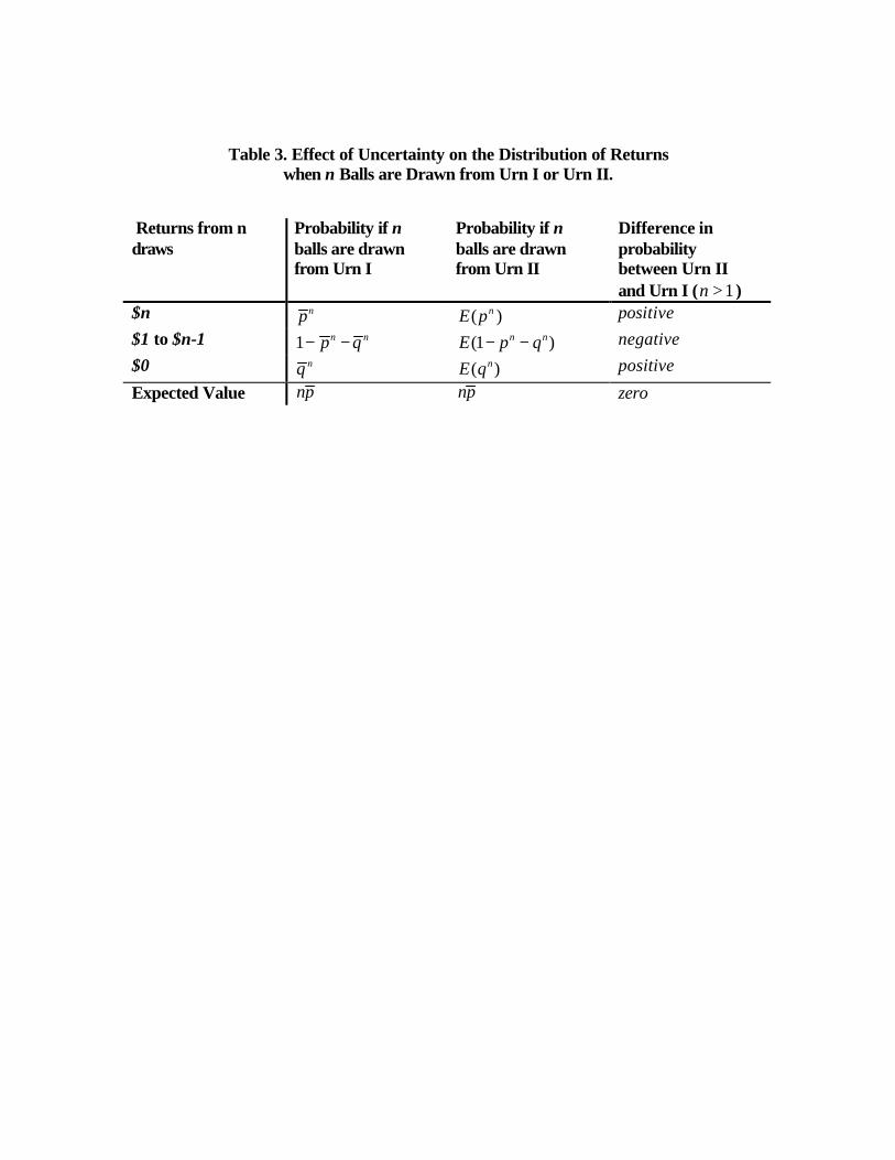
Table 3. Effect of Uncertainty on the Distribution of Returns when n Balls are Drawn from Urn I or Urn II.

Returns from n draws

Probability if n balls are drawn from Urn I

Probability if n balls are drawn from Urn II

Difference in probability between Urn II and Urn I ( 1n > )

$n np ( )nE p positive $1 to $n-1 1 n np q− − (1 )n nE p q− − negative $0 nq ( )nE q positive

Expected Value np np zero

Table 4. Descriptive Statististics for the Samples used in Tables 5 and 6

Number of Observations

MeanStandard Deviation Mean

Standard Deviation

Dependent Variable 0.2674 0.3371 0.0488 0.2373

Fraction of Exact Answers 0.3127 0.2183 0.4185 0.1552

Fraction of Answers at .5 0.1475 0.1218 0.1884 0.0827

Log of Net Worth 10.2178 3.2532 10.8156 1.8332

1998 Zero or Negative Net Worth 0.0541 0.2263

Single Female 0.3279 0.4695 0.1770 0.3818

Single Male 0.1275 0.3335 0.0745 0.2626

Household Age 68.0715 10.4612 56.7053 4.7905

Hispanic 0.0512 0.2205 0.0630 0.2430

Black 0.1282 0.3343 0.1222 0.3275

Education 12.1850 2.9737 12.6174 2.6673

Immediate Word Recall 5.3768 1.8125 7.7522 2.2281

Delayed Word Recall 4.3212 2.0670 5.7183 2.4321

Note: Variables used in Table 4 use 1998 data, those used in Table 5 use 1992 data.

Table 4. Determinants of Fraction of Total Assets

which are Risky

Table 5. Determinants of Average Yearly Percentage Change in Net

Worth

12339 4174

Table 5. Determinants of Share of Risky Assets in Portfolio in 1998*

Share of Total Assets** which are Risky (1a) (2a) (1b) (2b) Fraction of Exact Answers 0.0536 0.0498 0.0470 0.0441 (4.215) (3.848) (3.622) (3.334) Fraction of Answers at .5 -0.0216 -0.0244 (-0.997) (-1.125) Log of 1998 Net Worth** 0.0817 0.0818 0.0804 0.0805 (63.614) (63.472) (58.117) (58.078) Zero or Negative Net Worth** 0.6330 0.6336 0.6227 0.6232 (36.508) (36.521) (34.871) (34.888) Single Female 0.1264 0.0126 0.0092 0.0090 (2.131) (2.117) (1.512) (1.486) Single Male 0.0072 0.0069 0.0064 0.0061 (0.908) (0.0875) (0.808) (0.769) Household Age, 1998 -0.0034 -0.0035 -0.0032 -0.0033 (-12.826) (-12.622) (-10.999) (-10.955) Hispanic 0.0043 0.0038 0.0097 0.0092 (0.367) (0.319) (0.806) (0.763) Black 0.0027 0.0023 0.0045 0.0041 (0.346) (0.290) (0.570) (0.512) Education 0.0016 0.0017 (1.586) (1.623) Immediate Word Recall 0.0026 0.0026 (1.056) (1.060) Delayed Word Recall 0.0003 0.0003 (0.135) (0.153) Constant -0.3896 -0.3815 -0.4256 -0.4172 (-16.181) (-15.028) (-15.417) (-14.593) Number of Observations 12,339 12,339 12,339 12,339 Adjusted R-Squared 0.3119 0.3119 0.3121 0.3121

**t-values in parentheses. **Without housing equity.

Table 6. Determinants of Growth of Assets from 1992 to 1998*

Yearly Percent Change in Net Worth** (1a) (2a) (1b) (2b) Fraction of Exact Answers 0.2023 0.2111 0.1000 0.1117 (8.828) (8.847) (4.199) (4.527) Fraction of Answers at .5 0.0572 0.0766 (1.327) (1.804) Log of 1992 Net Worth** -0.0479 -0.0480 -0.0584 -0.0585 (-23.692) (-23.723) (-27.454) (-27.508) Single Female -0.0749 -0.0747 -0.0960 -0.0958 (-7.921) (-7.899) (-10.094) (-10.078) Single Male -0.0343 -0.0334 -0.0534 -0.0521 (-2.603) (-2.525) (-4.038) (-3.932) Household Age, 1992 -0.0012 -0.0011 -0.0003 -0.0002 (-1.695) (-1.564) (-0.378) (-0.210) Hispanic -0.1274 -0.1262 -0.0696 -0.0678 (-8.809) (-8.710) (-4.702) (-4.575) Black -0.0856 -0.0841 -0.0775 -0.0756 (-7.864) (-7.693) (-7.179) (-6.971) Education 0.0208 0.0209 (13.316) (13.346) Immediate Word Recall 0.0004 0.0005 (0.185) (0.231) Delayed Word Recall 0.0016 0.0016 (0.784) (0.744) Constant 0.5868 0.5676 0.4132 0.3871 (12.355) (11.435) (8.412) (7.562) Number of Observations 4,174 4,174 4,131 4,131 Adjusted R-Squared 0.1374 0.1376 0.1751 0.1756

*t-values in parentheses. **Without housing equity.

Fra

ctio

n

Social Security To Be Less Generous0 50 100

0

.1

.2

Fra

ctio

n

Double-Digit Inflation0 50 100

0

.1

.2

.3

Fra

ctio

n

Will Live To Be 750 50 100

0

.1

.2

.3

Fra

ctio

n

Income Will Keep Up With Inflation0 50 100

0

.1

.2

.3

Fra

ctio

n

Will Leave Inheritance >=10,0000 50 100

0

.2

.4

.6

Fra

ctio

n

Will Work At Age 620 50 100

0

.1

.2

.3

Figure 1. Histograms of Probability Responses in HRS

A. General Events

Social Security lessgenerous

Double digit inflation

B. Events with Personal Information

Survival to 75Income increase

faster than inflation

C. Events with Personal Control

Leave inheritanceWork at age 62

Figure 2. Distribution of Prior Probabilitieswith Varying Expected Values and Precision.

.01

.10

.50

.75

1.00

2.00

5.00

10.00

100.00

δσD

egre

e of

Impr

ecis

ion

xβ-2.0.022

-1.0.158

-.5.309

-.25.401

0.500

.25

.599.5.691

1.0.841

2.0.978

( )p F xβ=

Expected Value

0.1 .2.3 .4.5.6 .7.8 .9 10

0 .1.2 .3.4 .5.6.7 .8.9 10

0.1 .2.3 .4.5.6 .7.8 .9 10

0.1.2 .3.4.5 .6.7 .8.9 10

0.1 .2.3 .4.5 .6.7.8 .9 10

0 .1.2 .3.4 .5.6.7 .8.9 10

0.1 .2.3 .4.5 .6.7 .8.9 10

0.1.2 .3.4 .5.6 .7.8.9 10

0 .1.2.3 .4.5 .6.7.8 .9 10

0.1 .2.3 .4.5.6 .7.8 .9 10

0 .1.2 .3.4 .5.6.7 .8.9 10

0.1 .2.3 .4.5.6 .7.8 .9 10

0.1.2 .3.4.5 .6.7 .8.9 10

0.1 .2.3 .4.5 .6.7.8 .9 10

0 .1.2 .3.4 .5.6.7 .8.9 10

0.1 .2.3 .4.5 .6.7 .8.9 10

0.1.2 .3.4 .5.6 .7.8.9 10

0 .1.2.3 .4.5 .6.7.8 .9 10

0.1 .2.3 .4.5.6 .7.8 .9 1

0

0 .1.2 .3.4 .5.6.7 .8.9 1

0

0.1 .2.3 .4.5.6 .7.8 .9 1

0

0.1.2 .3.4.5 .6.7 .8.9 1

0

0.1 .2.3 .4.5 .6.7.8 .9 1

0

0 .1.2 .3.4 .5.6.7 .8.9 1

0

0.1 .2.3 .4.5 .6.7 .8.9 1

0

0.1.2 .3.4 .5.6 .7.8.9 1

0

0 .1.2.3 .4.5 .6.7.8 .9 1

0

0.1 .2.3 .4.5.6 .7.8 .9 1

0

0 .1.2 .3.4 .5.6.7 .8.9 1

0

0.1 .2.3 .4.5.6 .7.8 .9 1

0

0.1.2 .3.4.5 .6.7 .8.9 1

0

0.1 .2.3 .4.5 .6.7.8 .9 1

0

0 .1.2 .3.4 .5.6.7 .8.9 1

0

0.1 .2.3 .4.5 .6.7 .8.9 1

0

0.1.2 .3.4 .5.6 .7.8.9 1

0

0 .1.2.3 .4.5 .6.7.8 .9 1

0

0.1 .2.3 .4.5.6 .7.8 .9 10

0 .1.2 .3.4 .5.6.7 .8.9 10

0.1 .2.3 .4.5.6 .7.8 .9 10

0.1.2 .3.4.5 .6.7 .8.9 10

0.1 .2.3 .4.5 .6.7.8 .9 10

0 .1.2 .3.4 .5.6.7 .8.9 10

0.1 .2.3 .4.5 .6.7 .8.9 10

0.1.2 .3.4 .5.6 .7.8.9 10

0 .1.2.3 .4.5 .6.7.8 .9 10

0.1 .2.3 .4.5.6 .7.8 .9 10

0 .1.2 .3.4 .5.6.7 .8.9 10

0.1 .2.3 .4.5.6 .7.8 .9 10

0.1.2 .3.4.5 .6.7 .8.9 10

0.1 .2.3 .4.5 .6.7.8 .9 10

0 .1.2 .3.4 .5.6.7 .8.9 10

0.1 .2.3 .4.5 .6.7 .8.9 10

0.1.2 .3.4 .5.6 .7.8.9 10

0 .1.2.3 .4.5 .6.7.8 .9 10

0.1 .2.3 .4.5.6 .7.8 .9 1

0

0 .1.2 .3.4 .5.6.7 .8.9 1

0

0.1 .2.3 .4.5.6 .7.8 .9 1

0

0.1.2 .3.4.5 .6.7 .8.9 1

0

0.1 .2.3 .4.5 .6.7.8 .9 1

0

0 .1.2 .3.4 .5.6.7 .8.9 1

0

0.1 .2.3 .4.5 .6.7 .8.9 1

0

0.1.2 .3.4 .5.6 .7.8.9 1

0

0 .1.2.3 .4.5 .6.7.8 .9 1

0

0.1 .2.3 .4.5.6 .7.8 .9 1

0

0 .1.2 .3.4 .5.6.7 .8.9 1

0

0.1 .2.3 .4.5.6 .7.8 .9 1

0

0.1.2 .3.4.5 .6.7 .8.9 1

0

0.1 .2.3 .4.5 .6.7.8 .9 1

0

0 .1.2 .3.4 .5.6.7 .8.9 1

0

0.1 .2.3 .4.5 .6.7 .8.9 1

0

0.1.2 .3.4 .5.6 .7.8.9 1

0

0 .1.2.3 .4.5 .6.7.8 .9 1

0

0.1 .2.3 .4.5.6 .7.8 .9 10

0 .1.2 .3.4 .5.6.7 .8.9 10

0.1 .2.3 .4.5.6 .7.8 .9 10

0.1.2 .3.4.5 .6.7 .8.9 10

0.1 .2.3 .4.5 .6.7.8 .9 10

0 .1.2 .3.4 .5.6.7 .8.9 10

0.1 .2.3 .4.5 .6.7 .8.9 10

0.1.2 .3.4 .5.6 .7.8.9 10

0 .1.2.3 .4.5 .6.7.8 .9 10

Figure 3. Relation Between Prior Distribution and Heaping under Modal Choice Hypothesis.

.01

.10

.50

.75

1.00

2.00

5.00

10.00

100.00

δσD

egre

e of

Impr

ecis

ion

xβ-2.0.022

-1.0.158

-.5.309

-.25.401

0.500

.25

.599.5.691

1.0.841

2.0.978 * ( )p F xβ=

Expected Value

D. Answer = 50Distribution is Unimodal at .5 orBimodal with ApproximatelyEqual Modes at 0 and 1.

A. Answer = Exact ValueDistribution is Unimodalfor some 0<mode<1

B. Answer = 0DistributionHas largestmode atzero

C. Answer = 100DistributionHas largestmode at one

Figure 4. Mean Focal Answers vs. Predicted Probabilities

Me

an

Fo

ca

l A

nsw

er

Centile of Predicted Probability

SOC.SEC. MORE GENEROUS.1 .5

.1

.5

SOC.SEC. LESS GENEROUS.45 .7

.45

.7

ECONOMIC DEPRESSION.45 .75

.45

.75

INFLATION.5 .75

.5

.75

SURVIVAL TO 75.45 .85

.45

.85

SURVIVAL TO 85.35 .7

.35

.7

GIVE HELP.2 .65

.2

.65

WILL WORK AT 62.2 .75

.2

.75

HEALTH WILL LIMIT WORK.25 .5

.25

.5

Mean F

ocal A

nsw

er

Centile of Predicted Probability

SOC.SEC. MORE GENEROUS.1 .55

.1

.55

SOC.SEC. LESS GENEROUS.45 .7

.45

.7

ECONOMIC DEPRESSION.45 .65

.45

.65

INFLATION.5 .7

.5

.7

SURVIVAL TO 75.5 .85

.5

.85

SURVIVAL TO 85.35 .65

.35

.65

GIVE HELP.3 .5

.3

.5

WILL WORK AT 62.2 .7

.2

.7

HEALTH WILL LIMIT WORK.25 .5

.25

.5

A. Prediction Based on Full Sample, 1992 B. Prediction Based on Sample with Exact Answers, 1992M

ean F

ocal A

nsw

er

Centile of Predicted Probability

SOC.SEC. LESS GENEROUS.4 .75

.4

.75

ECONOMIC DEPRESSION.3 .48

.3

.48

INFLATION.35 .58

.35

.58

SURVIVAL TO 75.4 .8

.4

.8

SURVIVAL TO 85.3 .7

.3

.7

GO TO NURSING HOME.02 .5

.02

.5

GIVE HELP0 .8

0

.8

RECEIVE HELP0 .2

0

.2

LEAVE INHERITANCE 1.1 1

.1

1

LEAVE INHERITANCE 20 1

0

1

LEAVE ANY INHERITANCE0 .4

0

.4

RECEIVE INHERITANCE0 .5

0

.5

INCOME KEEP UP W/ INFLATION.25 .7

.25

.7

WILL WORK SOMETIMES0 .6

0

.6

WILL WORK AT 62.15 .75

.15

.75

HEALTH WILL LIMIT WORK.2 .55

.2

.55

Mean F

ocal A

nsw

er

Centile of Predicted Probability

SOC.SEC. LESS GENEROUS.4 .75

.4

.75

ECONOMIC DEPRESSION.3 .48

.3

.48

INFLATION.3 .55

.3

.55

SURVIVAL TO 75.4 .8

.4

.8

SURVIVAL TO 85.3 .65

.3

.65

GO TO NURSING HOME.05 .5

.05

.5

GIVE HELP0 .8

0

.8

RECEIVE HELP0 .4

0

.4

LEAVE INHERITANCE 1.15 1

.15

1

LEAVE INHERITANCE 20 .9

0

.9

LEAVE ANY INHERITANCE0 .5

0

.5

RECEIVE INHERITANCE0 .6

0

.6

INCOME KEEP UP W/ INFLATION.25 .7

.25

.7

WILL WORK SOMETIMES0 .6

0

.6

WILL WORK AT 62.2 .7

.2

.7

HEALTH WILL LIMIT WORK.2 .55

.2

.55

C. Prediction Based on Full Sample, 1998 D. Prediction Based on Sample with Exact Answers, 1998

Figure 5. Analysis of Focal and Exact Answers to Sunny Question Using Interview Responses Grouped by Month and PSU.

Frac

tion

of A

nsw

ers

Probability Tomorrow will Be Sunny

Fraction Exact

0 .25 .5 .75 1

0

.25

.5

.75

1Fraction Not 50-50

0 .25 .5 .75 1

0

.25

.5

.75

1

Fraction 0

0 .25 .5 .75 1

0

.25

.5

.75

1Fraction 100

0 .25 .5 .75 1

0

.25

.5

.75

1

HRS 1994AHEAD 1993/95

HRS 1994

AHEAD 1993/95

HRS 1994AHEAD 1993/95

HRS 1994

AHEAD 1993/95

Figure 6. Distribution of Fraction of ExactAnswers to Subjective Probability Questions

in HRS-1998.

Fra

ctio

n

Fraction Exact Answers0.000 1.000

0.000

0.142

Figure 7. Propensity to Give Exact Answers toSubjective Probability Questions by Age and Education

50 60 70 80 90 100 110

0

.1

.2

.3

.4

.5

0 6 12 16 17

0

.1

.2

.3

.4

.5

Age Education

Frac

tion

Exa

ct A

nsw

ers

Table 5A. Determinants of Share of Risky Assets in Portfolio in 1998* Controlling for SSA Lifetime Earnings

Share of Total Assets** which are Risky

(3a) (4a) (3b) (4b) (3c) (4c) (3d) (4d)

Fraction of Exact Answers 0.0696 0.0678 0.0644 0.0622 0.0706 0.0686 0.0654 0.0630 (3.486) (3.322) (3.133) (2.957) (3.524) (3.349) (3.175) (2.988) Fraction of Answers at .5 -0.0150 -0.0177 -0.0163 -0.0189 (-0.420) (-0.493) (-0.452) (-0.527) Log of 1998 Net Worth** 0.0909 0.0909 0.0902 0.0902 0.0907 0.0908 0.0901 0.0901 (41.659) (41.584) (38.391) (38.366) (39.517) (39.480) (37.044) (37.034) Zero or Negative N.Worth** 0.7249 0.7252 0.7194 0.7196 0.7239 0.7241 0.7191 0.7192 (25.740) (25.740) (24.765) (24.767) (25.124) (25.126) (24.336) (24.337) Single Female 0.0157 0.0156 0.0125 0.0123 0.0169 0.0169 0.0129 0.0128 (1.154) (1.503) (1.167) (1.149) (1.510) (1.509) (1.114) (1.107) Single Male 0.0305 0.0303 0.02831 0.0280 0.0304 0.0302 0.0278 0.0275 (2.239) (2.221) (2.071) (2.048) (2.202) (2.183) (2.001) (1.978) Household Age, 1998 -0.0034 -0.0034 -0.0033 -0.0034 -0.0033 -0.0034 -0.0033 -0.0033 (-4.138) (-4.150) (-4.024) (-4.051) (-4.091) (-4.109) (-3.963) (-3.996) Hispanic 0.0202 0.0197 0.0260 0.0256 0.0213 0.0209 0.0268 0.0264 (1.204) (1.174) (1.501) (1.473) (1.254) (1.225) (1.532) (1.505) Black 0.0031 0.0027 0.0036 0.0031 0.0043 0.0039 0.0047 0.0043 (0.242) (0.209) (0.277) (0.240) (0.338) (0.303) (0.368) (0.329) Education 0.0012 0.0012 0.0012 0.0012 (0.641) (0.655) (0.660) (0.675) Immediate Word Recall 0.0106 0.0106 0.0105 0.0105 (2.491) (2.499) (2.469) (2.477) Delayed Word Recall -0.0077 -0.0077 -0.0075 -0.0075 (-2.048) (-2.047) (-1.995) (-1.995) 2nd Earnings Decile -0.0194 -0.0189 -0.0180 -0.0174 (-0.833) (-0.858) (-0.818) (-0.789) 3rd Earnings Decile -0.0284 -0.0280 -0.0278 -0.0273 (-1.323) (-1.301) (-1.295) (-1.270) 4th Earnings Decile -0.0030 -0.0022 -0.0030 -0.0021 (-0.139) (-0.103) (-0.139) (-0.098) 5th Earnings Decile -0.0161 -0.0157 -0.0165 -0.0160 (-0.750) (-0.730) (-0.766) (-0.743) 6th Earnings Decile -0.0119 -0.0112 -0.0120 -0.0112 (-0.552) (-0.518) (-0.558) (-0.520) 7th Earnings Decile 0.0036 0.0044 0.0037 0.0046 (0.167) (0.201) (0.171) (0.211) 8th Earnings Decile -0.0085 -0.0076 -0.0101 -0.0093 (-0.386) (-0.353) (-0.460) (-0.422) 9th Earnings Decile -0.0042 -0.0037 -0.0061 -.0055 (-0.191) (-0.168) (-0.274) (-0.247) 10th Earnings Decile -0.0206 -0.0199 -0.0223 -0.0216 (-0.922) (-0.890) (-0.999) (-0.963) Constant -0.4978 -0.4916 -0.5305 -0.5237 -0.4877 -0.4816 -0.5223 -0.5156 (-8.625) (-8.249) (-8.759) (-8.425) (-8.058) (-7.761) (-8.233) (-7.965)

Number of Observations 4,365 4,365 4,365 4,365 4,365 4,365 4,365 4,365 Adjusted R-Squared 0.3509 0.3508 0.3515 0.3514 0.3504 0.3503 0.3510 0.3509 **t-values in parentheses. **Without housing equity.

Table 6A. Determinants of Growth of Assets from 1992 to 1998* Controlling for SSA Lifetime Earnings

Yearly Percent Change in Net Worth**

(3a) (4a) (3b) (4b) (3c) (4c) (3d) (4d)

Fraction of Exact Answers 0.2162 0.2288 0.1059 0.1199 0.1936 0.2039 0.0965 0.1083 (8.206) (8.362) (3.849) (4.220) (7.404) (7.500) (3.532) (3.833) Fraction of Answers at .5 0.0850 0.0961 0.0684 0.0799 (1.696) (1.955) (1.379) (1.635) Log of 1992 Net Worth** -0.0474 -0.0475 -0.0575 -0.0576 -0.0531 -0.0532 -0.0615 -0.0616 (-20.465) (-20.506) (-23.706) (-23.757) (-22.469) (-22.491) (-25.068) (-25.097) Single Female -0.0815 -0.0814 -0.1011 -0.1010 -0.0238 -0.0243 -0.0491 -0.0497 (-7.574) (-7.563) (-9.369) (-9.358) (-1.904) (-1.940) (-3.892) (-3.938) Single Male -0.0512 -0.0499 -0.0680 -0.0663 -0.0167 -0.0158 -0.0372 -0.0360 (-3.427) (-3.336) (-4.561) (-4.445) (-1.099) (-1.037) (-2.439) (-2.358) Household Age, 1998 -0.0011 -0.0010 -0.0002 -0.0001 -0.0014 -0.0013 -0.0006 -0.0005 (-1.376) (-1.212) (-0.290) (-0.109) (-1.754) (-1.620) (-0.718) (-0.556) Hispanic -0.1293 -0.1269 -0.0727 -0.0699 -0.1005 -0.0988 -0.0528 -0.0506 (-7.489) (-7.332) (-4.148) (-3.974) (-5.796) (-5.684) (-3.005) (-2.875) Black -0.0956 -0.0932 -0.0875 -0.0847 -0.0925 -0.0905 -0.0854 -0.0831 (-7.256) (-7.031) (-6.717) (-6.469) (-7.100) (-6.909) (-6.611) (-6.397) Education 0.0211 0.0211 0.0193 0.0194 (11.758) (11.764) (10.799) (10.806) Immediate Word Recall -0.0004 -0.0002 -0.0011 -0.0009 (-0.162) (-0.087) (-0.396) (-0.332) Delayed Word Recall 0.0019 0.0018 0.0023 0.0022 (0.815) (0.763) (0.957) (0.913) 2nd Earnings Decile 0.0064 0.0052 0.0086 0.0070 (0.282) (0.227) (0.384) (0.312) 3rd Earnings Decile 0.0212 0.0201 0.0232 0.0217 (0.963) (0.909) (1.066) (0.994) 4th Earnings Decile 0.0433 0.0453 0.0439 0.0416 (1.961) (1.877) (2.012) (1.906) 5th Earnings Decile 0.0743 0.0727 0.0710 0.0690 (3.343) (3.268) (3.240) (3.144) 6th Earnings Decile 0.0584 0.0563 0.0536 0.0510 (2.643) (2.554) (2.460) (2.336) 7th Earnings Decile 0.0868 0.0847 0.0790 0.0764 (3.937) (3.834) (3.631) (3.500) 8th Earnings Decile 0.1079 0.1056 0.0985 0.0956 (4.808) (4.694) (4.450) (4.308) 9th Earnings Decile 0.1315 0.1300 0.1183 0.1161 (5.815) (5.734) (5.299) (5.195) 10th Earnings Decile 0.1557 0.1539 0.1363 0.1340 (6.898) (6.806) (6.113) (5.997) Constant 0.5720 0.5438 0.4033 0.3707 0.5635 0.5423 0.4076 0.3825 (10.558) (9.599) (7.224) (6.366) (9.982) (9.274) (7.000) (6.351)

Number of Observations 3,133 3,133 3,111 3,111 3,133 3,133 3,111 3,111 Adjusted R-Squared 0.1407 0.1412 0.1792 0.1799 0.1648 0.1650 0.1963 0.1968 **t-values in parentheses. **Without housing equity.