Embed Size (px)
Citation preview

Software for computer-aided design of single and double-pipe central heating
and hydronic radiant heating systems
Version 4
© InstalSoft 2005

Rev. 2005-06-02

Foreword THE PRODUCER OF THIS SOFTWARE APPLICATIONS SHALL NOT BE LIABLE FOR LOSS OF PROFITS OR INCOME, LOSS OF DATA, DAMAGE OF EQUIPMENT OR ANY OTHER LOSS ARISING OUT OF THE USE OF THIS SOFTWARE.
The software application presented in this manual is protected by
Copyright. The User is therefore obliged not to distribute or duplicate this application.
The software Copyright owner is InstalSoft s.c.. Legal purchasers of the
software are entitled to obtain explanations regarding its use. The authors shall not be liable for the consequences of wrong installation
of the software, abuse or calculation results.
Contact with the authors: http://www.instalsoft.com.pl
Trademarks: InstalSoft, InstalSystem, Gredi, OZC are registered trademarks of InstalSoft s.c. or of their proprietors. Adobe and Acrobat are trademarks of Adobe Systems Incorporated. AutoCAD is a registered trademark of Autodesk, Inc. Microsoft is a registered trademark of Microsoft Corporation. Names of installation products are used in this manual for illustrative purposes only and they do not constitute any recommendation for particular applications and guarantee of presence of these products in catalogues included in the software.


I
Contents:
1. INTRODUCTION .................................................................................................1 1.1. PURPOSE AND FEATURES ..................................................................................1 1.2. COMMUNICATION WITH OTHER APPLICATIONS OF THE INSTALSYSTEM
PACKAGE..........................................................................................................2 1.3. COMMUNICATION WITH OTHER ENGINEERING SOFTWARE .....................................3 1.4. ARRANGEMENT OF THE MANUAL ........................................................................3 1.5. SYMBOLS USED ................................................................................................3 1.6. TERMS AND ABBREVIATIONS USED .....................................................................4
2. SHORT DESCRIPTION OF THE STAGES OF CREATING A TYPICAL PROJECT .................................................................................................7
2.1. INTRODUCTION .................................................................................................7 2.2. CREATING PLANS OF STOREYS AS BASE FOR PROJECT ........................................7
2.2.1. Drawing floor plan in the application ..................................................7 2.2.2. Importing plan view from a DWG/DXF file........................................10
2.3. FLOOR HEATING DESIGN (ON PLAN VIEWS) ........................................................11 2.3.1. Stages of creating a project..............................................................11 2.3.2. Creating a new project .....................................................................12 2.3.3. Specifying room data........................................................................12 2.3.4. Editing the floor heating system .......................................................13 2.3.5. Data diagnostics...............................................................................17 2.3.6. Determination of supply temperature ...............................................17 2.3.7. Analysis of calculation results and messages ..................................17 2.3.8. Data correction, HZ division, drawing pipe feeds .............................18 2.3.9. Repeated data diagnostics and analysis of results ..........................21 2.3.10. Analysis of complete results and printout.........................................21
2.4. RADIATOR HEATING DESIGN (PLAN VIEWS AND SCHEMATIC VIEW) .......................22 2.4.1. Stages of creating a project..............................................................22 2.4.2. Creating a new project .....................................................................23 2.4.3. Placing radiators and distribution network........................................23 2.4.4. Opening a schematic view sheet of the system ...............................24 2.4.5. Associating radiators and pipe-runs (originals – shadows) ..............26 2.4.6. Appending data and selecting component types..............................26 2.4.7. Specifying calculation options, diagnostics and running
calculations ......................................................................................28 2.4.8. Analysis of complete results and project printout .............................29
3. PROJECT AND ITS DATA ...............................................................................31 3.1. GENERAL INFORMATION ON THE STRUCTURE OF PROJECT DATA.........................31
3.1.1. Drawing sheets ................................................................................32 3.1.2. Components that form project on sheets .........................................32
3.2. ASSOCIATIONS BETWEEN PLAN VIEWS AND SCHEMATIC VIEWS............................34 3.3. CREATE A NEW PROJECT .................................................................................34 3.4. PROJECT OPTIONS ..........................................................................................35
3.4.1. “Info” tab...........................................................................................35 3.4.2. “General data” tab ............................................................................35 3.4.3. “Default types” tab............................................................................36 3.4.4. “Building structure” tab .....................................................................37

II
3.4.5. “Radiant heating” tab....................................................................... 37 3.4.6. “Edit” tab.......................................................................................... 40
3.5. CATALOGUE SELECTION ................................................................................. 40 3.6. SAVING A PROJECT TO DISK AND LOADING A PROJECT FROM DISK ...................... 41 3.7. AUTOSAVE FEATURE ...................................................................................... 42 3.8. WORKSHEETS IN FILE ..................................................................................... 42
4. GRAPHICAL EDITOR FUNDAMENTALS....................................................... 45 4.1. INTRODUCTION .............................................................................................. 45 4.2. SCREEN COMPONENTS................................................................................... 45 4.3. MOVING AROUND THE PROJECT – VIEWING AND SCALE ..................................... 48 4.4. MOVING AROUND THE PROJECT - NAVIGATOR................................................... 50 4.5. PROJECT LAYERS........................................................................................... 51 4.6. OPERATING MODES OF THE EDITOR: AUTO, LOCK, GRID, ORTO, REP.......... 51
4.6.1. ORTO mode - Inserting horizontal and vertical components........... 51 4.6.2. LOCK mode – Locking components................................................ 54 4.6.3. GRID mode – Drawing grid ............................................................. 55 4.6.4. AUTO mode – Automatic component connecting ........................... 56 4.6.5. REP mode – Repetitive insertion of components ............................ 58
4.7. UNDO AND REDO............................................................................................ 59 4.8. INSERTING COMPONENTS AND OPERATIONS PERFORMED ON
COMPONENTS ................................................................................................ 60 4.8.1. Inserting components ...................................................................... 60 4.8.2. Marking single components............................................................. 61 4.8.3. Marking multiple components.......................................................... 62 4.8.4. Marking multiple components with the use of the Shift key............. 62 4.8.5. Marking multiple components within a specified area ..................... 63 4.8.6. Marking multiple components of specified type in the entire sheet . 64 4.8.7. Moving component .......................................................................... 64 4.8.8. Flipping a component horizontally ................................................... 65 4.8.9. Changing the dimensions of components ....................................... 65 4.8.10. Rotating a component ..................................................................... 66 4.8.11. Deleting components....................................................................... 67 4.8.12. Disconnecting components ............................................................. 67 4.8.13. Repeated inserting of an identical component ................................ 67
4.9. APPENDING COMPONENT DATA ....................................................................... 68 4.9.1. Data appending fundamentals......................................................... 68 4.9.2. Data table field types and editing .................................................... 68 4.9.3. Specifying types. Letter shortcuts.................................................... 70 4.9.4. Local resistance components .......................................................... 72 4.9.5. Repeated entering of the same data ............................................... 73 4.9.6. Repeating the last value.................................................................. 73 4.9.7. Simultaneous entering of data for multiple components.................. 73 4.9.8. Data sets and data sets gallery ....................................................... 74 4.9.9. Moving between components using the keyboard .......................... 76
4.10. HARDWARE AND FITTINGS.......................................................................... 77 4.10.1. Basic information............................................................................. 77 4.10.2. Inserting single fitting components .................................................. 77 4.10.3. Deleting fitting components ............................................................. 78 4.10.4. Inserting multiple fittings.................................................................. 78 4.10.5. Appending fitting component data ................................................... 79 4.10.6. Selecting the manner of drawing fitting components....................... 79

III
4.11. INSERTING AND CONFIGURING PIPE-RUN LABELS ..........................................81 4.12. CONNECTION POINTS .................................................................................82
5. COMPONENTS OF THE BASE BUILDING DRAWING...................................83 5.1. INTRODUCTION ...............................................................................................83 5.2. COMPONENTS OF A STOREY PLAN VIEW ............................................................83
5.2.1. Wall ..................................................................................................84 5.2.2. Curved wall ......................................................................................85 5.2.3. Opening in wall.................................................................................87 5.2.4. Window ............................................................................................88 5.2.5. Door .................................................................................................89 5.2.6. Room................................................................................................90 5.2.7. Horizontal partition: floor ..................................................................94 5.2.8. Horizontal partition: ceiling ...............................................................96 5.2.9. Compass rose ..................................................................................97
5.3. EDITING PLAN VIEW .........................................................................................98 5.3.1. Basic rules........................................................................................98 5.3.2. Appending additional components to the construction...................100 5.3.3. Data of importance to floor heating design.....................................102 5.3.4. Complex cases encountered when editing construction ................103
5.4. ARRANGEMENT OF FLOORS IN A SCHEMATIC VIEW ...........................................104 6. COMPONENTS THAT MAKE UP THE SYSTEM DIAGRAM.........................107
6.1. BASIC COMPONENTS OF A RADIATOR HEATING SYSTEM....................................107 6.1.1. Radiator..........................................................................................107 6.1.2. Terminal unit with imposed pressure drop .....................................110 6.1.3. Heating riser ...................................................................................112 6.1.4. Pipe-run..........................................................................................113 6.1.5. Single-pipe connection ...................................................................115 6.1.6. By-pass pipe-run, pipe-run with no flow .........................................116 6.1.7. Manifold..........................................................................................116 6.1.8. Manifold with a distributor main......................................................118 6.1.9. Boiler and Source...........................................................................119 6.1.10. Remote connection ........................................................................121 6.1.11. Automatic schematic view..............................................................122 6.1.12. Riser as a drawing..........................................................................123 6.1.13. Three-way valve.............................................................................124 6.1.14. Four-way valve...............................................................................125 6.1.15. Mixer (temperature reducer)...........................................................127 6.1.16. Bypass bottle..................................................................................128 6.1.17. Expansion vessel ...........................................................................129 6.1.18. Fitting components placed on pipe-runs ........................................129 6.1.19. Fitting components placed on terminal units ..................................131 6.1.20. Fitting components placed on manifolds ........................................131 6.1.21. Pumps ............................................................................................132 6.1.22. Special components .......................................................................132
6.2. BASIC RADIANT HEATING UNITS IN THE SYSTEM ...............................................133 6.2.1. Heating floor...................................................................................133 6.2.2. Heating wall....................................................................................138 6.2.3. Manifold..........................................................................................141 6.2.4. Mixer (temperature reducer)...........................................................143 6.2.5. Pipe feed and pair of pipe feeds.....................................................143

IV
6.2.6. Radiant heating circuit ................................................................... 145 6.2.7. Floor heating manifold................................................................... 146 6.2.8. Polylines for depicting piping ......................................................... 148
6.3. INSERTING AND EDITING HEATING ZONES (HZ’S)............................................. 149 6.3.1. Pasting a HZ with a spacing from walls......................................... 149 6.3.2. Dividing a HZ................................................................................. 150 6.3.3. HZ that covers only part of room ................................................... 152
6.4. INSERTING MANIFOLDS AND MANIFOLD FITTINGS ............................................. 155 6.5. EDITING PIPE FEEDS..................................................................................... 157
6.5.1. Inserting pipe feeds in the drawing................................................ 157 6.5.2. Modifying existing pipe feeds ........................................................ 159 6.5.3. Pipe feed data table (as part of HZ table)...................................... 162 6.5.4. Pipe feeds in HZ’s heated by pipe feeds ....................................... 164
6.6. GRAPHICAL COMPONENTS AND LABELS.......................................................... 166 7. ADVANCED EDITING FUNCTIONS.............................................................. 169
7.1. SENDING AND OPENING PROJECTS WITH THE USE OF ELECTRONIC MAIL ........... 169 7.2. COMPONENT APPEARANCE CONFIGURATION .................................................. 170
7.2.1. Configuring the appearance of structural and heating system components................................................................................... 170
7.2.2. Configuring the appearance of radiator labels............................... 171 7.2.3. Component label layout configuration window .............................. 173
7.3. GRAPHICAL EDITOR CONFIGURATION ............................................................. 174 7.3.1. User settings ................................................................................. 175 7.3.2. Screen appearance configuration.................................................. 177 7.3.3. Configuring toolbars, keyboard, mouse and pop-up menu............ 178 7.3.4. Changing the sequence of data displayed in data table................ 182
7.4. USING DRAWINGS FROM OTHER APPLICATIONS............................................... 183 7.4.1. Importing drawings; Drawings gallery............................................ 183 7.4.2. Saving a fragment of project as a drawing .................................... 185 7.4.3. Using drawings.............................................................................. 186
7.5. IMPORTING DWG/DXF FILE AS PLAN WITH INTERPRETATION........................... 186 7.6. IMPORTING DWG/DXF FILE AS PLAN WITHOUT INTERPRETATION..................... 188 7.7. EXPORTING A DRAWING ................................................................................ 189 7.8. NUMBERING OF ROOMS ................................................................................ 191 7.9. DEFINING MACRODEFINITIONS....................................................................... 192 7.10. DUPLICATING FRAGMENTS OF THE PROJECT ............................................. 193
7.10.1. Copying to the clipboard and pasting ............................................ 193 7.10.2. Duplicating by means of expanding groups................................... 194 7.10.3. Duplicating drawing fragments in specified direction..................... 196
7.11. MODULES............................................................................................... 196 7.11.1. Modules - introduction ................................................................... 196 7.11.2. Creating and storing modules........................................................ 196 7.11.3. Modules gallery ............................................................................. 197 7.11.4. Configuring a module .................................................................... 197 7.11.5. Creating expanding groups ........................................................... 198
7.12. DRAWING PIPING SYSTEM WITHIN HEATING ZONES..................................... 199 7.12.1. Automatic drawing......................................................................... 199 7.12.2. Manual drawing ............................................................................. 200
7.13. GROUPING AND UNGROUPING .................................................................. 202 7.14. FINDING A COMPONENT ........................................................................... 203 7.15. WORKING ON TWO OR MORE PROJECTS SIMULTANEOUSLY......................... 204

V
7.16. AUTOREAD FILE....................................................................................204 8. DIAGNOSTICS AND CALCULATIONS..........................................................207
8.1. CALCULATION METHOD..................................................................................207 8.1.1. Distribution of heat loss ..................................................................207 8.1.2. Floor heating calculations...............................................................208 8.1.3. Heater sizing ..................................................................................212 8.1.4. Flow calculations and system adjustment ......................................213
8.2. INVOKING DATA DIAGNOSTIC AND CALCULATIONS ............................................214 8.3. DATA DIAGNOSTICS.......................................................................................214
8.3.1. Types and syntax of messages......................................................214 8.3.2. Checking connections ....................................................................215 8.3.3. Data diagnostics.............................................................................215 8.3.4. Finding the component or field to which a message applies ..........216
8.4. CALCULATION OPTIONS .................................................................................217 8.4.1. Determining supply temperatures for control circuits .....................218 8.4.2. Graph of fitting ts/θs and optimisation of ts/θs on the basis of the
graph ..............................................................................................219 8.4.3. Radiant heating calculation options................................................221 8.4.4. Other calculation options: diameter sizing......................................227 8.4.5. System balancing options ..............................................................228 8.4.6. Thermal calculation options............................................................229 8.4.7. Result editing options.....................................................................231
9. PRESENTATION OF CALCULATION RESULTS..........................................233 9.1. LIST OF MESSAGES PERTAINING TO CALCULATION RESULTS .............................233 9.2. TABLES OF RESULTS .....................................................................................233
9.2.1. General results for radiator heating................................................233 9.2.2. General results for radiant heating .................................................234 9.2.3. Table of pipe-runs ..........................................................................236 9.2.4. Table of terminal units ....................................................................237 9.2.5. Table of rooms ...............................................................................238 9.2.6. Table of results for radiant heating.................................................238 9.2.7. Table of assembly parameters of radiant heating ..........................241 9.2.8. Table of circuits ..............................................................................244 9.2.9. List of components on pipe-runs ....................................................245 9.2.10. List of components on terminal units..............................................245 9.2.11. Graph of thermal matching of convectors ......................................246 9.2.12. List of pipes, pipe fittings and couplings.........................................246 9.2.13. List of valves, fittings and pumps ...................................................246 9.2.14. List of radiators...............................................................................247 9.2.15. List of manifolds .............................................................................247 9.2.16. List of insulation .............................................................................247 9.2.17. List of radiant heating components ................................................247 9.2.18. Pipe summary ................................................................................248 9.2.19. Finding components .......................................................................248 9.2.20. Configuring table appearance ........................................................250
9.3. PRINTING RESULT TABLES AND EXPORTING TO A SPREADSHEET .......................251 9.3.1. Printing calculation results on a printer ..........................................251 9.3.2. General printout settings: ...............................................................253 9.3.3. Printout layouts – specify the range of results printed:...................254 9.3.4. Printout styles – specify colours, fonts, etc.: ..................................255

VI
9.3.5. Exporting calculation results to an MS Excel spreadsheet .......... 255 9.4. RESULTS IN GRAPHICAL EDITOR .................................................................... 255 9.5. LOOKING UP COMPONENT RESULTS IN HINT BUBBLES...................................... 256 9.6. PRINTING, PRINT OPTIONS AND PRINTER SETTINGS ......................................... 257
9.6.1. Printing and print options............................................................... 257 9.6.2. Printer settings .............................................................................. 259 9.6.3. Printing on continuous paper......................................................... 259
9.7. ERROR LIST IN GRAPHICAL EDITOR ................................................................ 261 9.8. METHODS OF ALTERING CALCULATION RESULTS ............................................. 261
9.8.1. Radiant heating – unsatisfactory heat calculation results.............. 261 9.8.2. Radiant heating – unsatisfactory flow calculation results .............. 263 9.8.3. Radiator heating – unsatisfactory sizing of diameters ................... 264 9.8.4. Radiator heating – radiators sized for an apartment are of different
heights........................................................................................... 264 9.8.5. Excessive available pressure at source ........................................ 264
A. APPENDIX A – DEFAULT OPERATIONS ASSIGNED TO KEYBOARD AND MOUSE BUTTONS .................................................................... 267
A.1. KEYBOARD: ................................................................................................. 267 A.2. MOUSE: ...................................................................................................... 269
B. APPENDIX B – ERROR MESSAGES ........................................................... 271 B.1. MESSAGES FOR COMPONENTS IN THE PROJECT.............................. 271
C. APPENDIX C – SCAN COMBINER ............................................................... 293 C.1. INTRODUCTION ............................................................................................ 293 C.2. GENERAL SCHEME OF USING THE APPLICATION .............................................. 293 C.3. RULES FOR SCANNING BASE DRAWING FRAGMENTS........................................ 293 C.4. OPERATIONS CARRIED OUT ON THE FIRST FRAGMENT OF BASE DRAWING ......... 294 C.5. APPENDING SUBSEQUENT FRAGMENTS OF THE BASE DRAWING ....................... 295 C.6. TRIMMING AND SCALING THE BASE DRAWING.................................................. 296

Introduction
1
1. INTRODUCTION
1.1. Purpose and features
Instal-therm is intended for designers, installers, maintenance engineers and operators of hydronic central heating systems with convectors (double- and single-pipe systems) and radiant heating systems (floor and wall heating systems). It also supports the design and adjustment of double-pipe cooling medium circuits in air-conditioning systems. The circulating medium may comprise water or any of the non-freezing mixtures defined in the program.
System calculations include:
- sizing of pipes and fittings, including calculations of systems with user-specified diameters for part of the system or for the entire system,
- automatic sizing of all couplings and pipe fittings necessary to complete the structure of connections and geometry of the system defined by diagrams and to make connections with fittings and terminal units,
- determination of settings of control components in the system, such as preset radiator and riser valves, pressure differential and flow regulating valves, throttling orifices,
- sizing of required head of pumps on pipe-runs or in mixing systems, - sizing of pipework insulation, - heat and flow calculations of heating surfaces with automatic determination of
optimum supply temperature, - sizing of radiators with allowance made for temperature drop in pipelines, heat
gains from pipe-runs and additional sources, - convector output adjusting calculations by altering water temperature drop and
heating medium flow, - bill of materials: pipes, pipe fittings and couplings, insulation, radiators, radiant
heating components, valves and other fittings. The range of calculations presented above applies to the complete version of
software, which is identified by the letters HCR which follow the name of the software. The software may also be supplied in versions that feature the calculations of:
- radiator heating systems (Instal-therm H), - radiator heating systems and cooling circuits (Instal-therm HC), - radiator and radiant surface heating systems (Instal-therm HR).
Irrespective of the version, the principal graphical environment and the user
interface of the software is the same. Only some of the calculation functions and associated options, as well as some components and catalogue types will not be available in individual versions of the software.
The following catalogues are required to enable working with the program:
- catalogues of pipes, pipe fittings and couplings, including associated fittings (valves, radiator connections) from the manufacturer,
- catalogues of convectors, - catalogues of radiant surface (floor or wall) heating systems with specifications
of all system components and all data required for calculations, including geometrical, heat and flow restrictions defined by the system manufacturer,

Introduction
2
- thermostatic and control valves, - catalogues of pipe insulation.
Catalogues are binary files prepared by InstalSoft and the user cannot modify
them. Some catalogues, e.g. of commonly used cut-off fittings, are not associated with any specific manufacturer. There is no limitation on the number of catalogues used simultaneously, except for the restrictions defined by the software use licence (full version or firmware – usually limited to a defined set of catalogues).
Bills of materials include all determined and specified sizes of components that
make up the system and sized components of radiant surface heating system, as well as pipe fittings and couplings that enable making connections between components.
Calculation results are presented both in the form of tables as well as on plans and developed view drawings, which form the input data.
The software is the continuation and integration of two applications present on the
market: Instal-c.h. i Instal-f.h. – version 2. It retains their features – calculation of a central heating system based only on a 2-D or isometric drawing of the system and calculation of a floor heating system (including manifold) based on plans only. *.cow and *.opw files are read by the program. It may, however, not be possible to make calculations immediately after loading these files, or the interpretation of these files may differ from that by version 2. Users who would like to recalculate files created with version 2 software will find information on the major differences in data interpretation in a table at the end of this manual.
1.2. Communication with other applications of the InstalSystem package
Instal-therm is a component of the InstalSystem package, which also include Instal-heat&energy for calculating heat losses and seasonal heat demand in buildings. Data exchange is made with the use of a data file, which is assigned to both Instal-therm and Instal-heat&energy. Heat losses of rooms calculated by the latter application are saved to the file with a distinction made of the so-called reduced heat losses (losses exclusive of heat loss across partitions that constitute the heating surfaces), enabling proper sizing of both convectors and radiant surface heating units. If radiators are sized by Instal-heat&energy, this information is also transferred to Instal-therm. The structure of the building (storeys, apartments and rooms) is recognised and presented by both applications in the same manner. When using base drawings made with CAD software and loaded onto Instal-therm by means of DWG or DXF files, it is possible to calculate heat losses in the building with Instal-heat&energy and then to make diagram and system calculations with Instal-therm.
The package is supplied with an application for scanning building plans and for
combining and rescaling these scanned plans. Files created with this application are in the form of bitmaps and they may be used to make a drawing background for drawing the plan of the heating system and also for drawing floor plan with the use of objects predefined in Instal-therm (walls, rooms, etc.).
Another component of the package is Instal-mat, which gathers information on
materials from one or more projects created with Instal-therm and Instal-san and on

Introduction
3
that basis draws up a collective bill of materials and materials order. At this stage the bill is appended with prices.
1.3. Communication with other engineering software
The base drawing (plans of individual storeys), which is necessary for designing radiant heating system and is also used to calculate heat losses, may be drawn directly in the application, or may be imported from one or more DXF or DWG files created with engineering graphical software. The files may be imported with or without having the walls, windows and doors interpreted. In the first case the individual objects are recognised and rooms will be defined. In the latter case the imported material will form just a background drawing on which the plan may be drawn. In order to enable proper interpretation of the file and identification of walls, windows and doors and creation of rooms, it is important that defined principles of graphical design are observed within the application where the building design is created. These principles are described further in this manual.
When plans and drawings and calculations of the system are complete, the
drawings with calculation results may be printed, or saved (exported) to DXF or DWG files. These files may include just the base drawing and the system, or the export may comprise the remaining contents of the DXF or DWG files from which the plans were imported, and then new layers will be appended with the components designed. This way the documents created may be adapted to a specific standard, where all graphical information (including other system drawings) is included in one DWG/DXF file.
1.4. Arrangement of the Manual
The sections of this Manual are arranged in a manner that enables a beginner to start working with the software right away and to let every user get acquainted with its advanced functions.
Section 2 describes shortly how to work with the software. The information given there is sufficient to start working with the program and to create projects with the use of its basic functions. The arrangement of information follows a typical scheme of creating a project.
Subsequent sections of the Manual describe all functions of the program arranged in a more encyclopaedic way. Information provided there is, to some extent, a repetition of what is included in section 2, but it is much more detailed.
Further parts of the Manual (section 3 and following sections) is also provided on
the installation disk of the software in the form of easy-to-browse HTML files and a PDF file, which enables printout of selected sections. Microsoft® Internet Explorer version 4 or higher is recommended to look through the Manual in the HTML format. To view or print the Manual in the PDF format, Adobe® Acrobat® Reader or Adobe® eBook Reader software is required.
1.5. Symbols used
The following symbols and abbreviation are used in the manual:

Introduction
4
Paragraphs marked with “♦” indicate lists of actions required for performing a
function. For instance:
♦ In order to place a component in the project: 1. Click the button on the toolbar representing the component. 2. Move the mouse pointer to the workspace. The mouse pointer takes the
shape of [...]. Paragraphs marked with an exclamation mark and printed in bold and italics
contain particularly important information. For instance:
! Double mouse click in the realtime zoom mode or “grabber hand” mode, toggles these modes on and off. This enables convenient and fast viewing of the project.
The following notation:
» command “File / Save project” (Ctrl+S, “Program” → ) « indicates the selection of the command “Save project” from the “File” menu. The
combination of Ctrl and S keys is the shortcut to this command – this means pressing the CTRL key, keeping it depressed and pressing the S key. This command can be
called from the “Program” toolbar by pressing the button.
1.6. Terms and abbreviations used
The following terms are used in this manual:
• Control circuit – heating zones, their pipe feeds and manifolds supplied with medium from one point (source or mixer) that provides defined supply temperature, which is sometimes lower than that defined for the remaining part of the installation, and which is determined during preliminary calculations for each individual circuit separately.
• Covering – the outermost layer (in contact with air in the room) of a heating floor,
distinguished for the sake of selecting a material by the designer.
• Data table – table in which component (one component or several components of the same type) data may be edited.
• Expanding group – a group with a defined manner of self-duplication (appending subsequent modules) effected when expanding the frame of such group.
• Fitting component – a component inserted in the diagram onto a pipe-run; may be a fitting in usual sense, e.g. a valve, or in a more general sense, e.g. a pipe elbow or bend (pipe fitting), fixed point or partition crossing.
• Group – a special type of module, having additional features, such as border (frame), beyond which the components of the group cannot be moved.

Introduction
5
• Installation – a set of interconnected heating or cooling medium circuits, terminal
units and fittings originating from one source. One project file may comprise several installations.
• Junction – a point in the diagram where a pipe-run is connected to a preceding or following pipe-run or pipe-runs, in the latter case resulting in the combining or distribution of the stream of medium.
• Layer – one of the planes displayed in the graphical editor, which together form a whole (Installation, Construction, Base).
• Mixer – set of fitting components and pipe-runs enabling partial mixing of return and feed media in order to lower the temperature of the latter, e.g. in radiant heating systems. Reduced to one symbol in the application.
• Module – a set of several interconnected components, available for multiple use on a toolbar.
• Partition build-up (structure, definition) – specification of thermal properties by enumerating the layers of building materials in the partition (available only in Instal-heat&energy). A partition may also be defined by specifying the heat transfer coefficient “U” or thermal resistance “R” (available in Instal-heat&energy and Instal-therm).
• Paste together area – area around a fitting component or terminal unit (pipe-run, elbow, valve, tee, etc.), where two adjacent components are deemed connected directly, that is with no pipe in between.
• Pipe feed – a pair of pipes connecting heating zone to the manifold, usually an extension of pipes that form radiant surface heating circuit.
• Pipe-run – a section of pipework that carries a defined, constant flux of medium.
• Pipe-run with no flow - a section of pipework where, under conditions adopted for calculations, no flow of medium occurs. An example is the pipe-run that connects to an expansion vessel.
• Remote connection – used to link two parts of a system placed on separate sheets or on one sheet. Remote connection can be used for pairs of pipe-runs and for single pipe-runs.
• Shadow – a component (terminal unit, pipe-run, source) duplicated in another worksheet and assigned to the original component, that is to an identical component in terms of its functions, drawn in the worksheet from which the complete structure of connections is loaded. These components are not tested for the correctness of their connections.
• Sheet – part of project included in one drawing board of the graphical editor (called “Section” in the previous version). Components drawn on one sheet of plan should

Introduction
6
make up the so-called one graphical storey. Every other sheet of plan constitutes another graphical storey.
• Single-pipe connection - a section of pipework within a single-pipe heating system structure, which connects in series radiators of that structure.
• Source – a point of external supply of the installation, a boiler room or a heat exchanger.
• Terminal unit – a component that receives heat energy from the installation and transfers it to the environment or to other medium (radiator, heating riser, ventilation heater) or vice versa (terminal unit in a cooling or air conditioning system).
Abbreviations are applied in the Manual and the program for names that are often
used:
Full name: Abbreviation:
Heating zone HZ Radiant heating RH, r.h. Output, heat loss Q/Φ Output, heat loss per 1 m2 q Heating floor or wall surface temperature tfs/θfs,
tws/θws Occupied (residential) zone OZ Peripheral (marginal) zone PZ Peripheral zone arranged by compacting pipe
arrangement cPZ
Peripheral zone arranged at the beginning of circuit, upstream of occupied zone
uPZ
Room temperature (depending on manufacturer) ti/θI Pipe spacing T
(B,b,p,r,VA) Temperature difference for heating zone ∆t/∆θ Supply temperature ts/θs Floor covering/lining heat resistance Rlb Required output of terminal units Qreq/Φreq Loss to be covered by radiant heating Qrh/Φrh Part of heat loss assigned to specific HZ Qrh/Φhz Loss to be covered by radiator heating Qrh/Φrad Valve on r.h. manifold, supply side s.v. Valve on r.h. manifold, return side r.v.

Short description of the stages of creating a typical project
7
2. SHORT DESCRIPTION OF THE STAGES OF CREATING A TYPICAL PROJECT
2.1. Introduction
In this section the basic stages of creating two types of projects are presented: radiant (floor) heating and radiator heating. First the methods are discussed of acquiring a storey plan, which may form a base for each of these projects. A detailed description of the many functions and mechanisms of the program is given in the following sections, to which reference is made in the subsections of this section.
2.2. Creating plans of storeys as base for project
A storey plan is in practice an indispensable component for designing a floor heating system, it is also often used in the design of radiator heating systems. Therefore we start explaining the process of creating a project with a description of the method of preparing such plan.
! If a building consists of many storeys and if we want to have a plan of each
storey in the project, a separate worksheet must be provided for each storey. The storey plan may be drawn directly in the application with the use of available
tools and objects, or it may be imported from a DXF or DWG file with walls, windows and doors identified. It is also possible to load a scanned drawing (or read in a DWG / DXF file as a drawing – without identification of walls, windows and doors) and obtain a background on which walls, windows and doors may be drawn with the use of available tools and objects or just the areas of individual rooms may be indicated. In this last case it will not be possible to directly calculate heat losses with Instal-heat&energy.
2.2.1. Drawing floor plan in the application
The plan view is drawn in the current sheet. If a new sheet has to be created, select “Worksheets” in the “File” menu and click on the “New” button, select sheet type (“Plan view” in this case) and click “OK” and then “Close”. The new sheet becomes the current sheet. Select the “Construction” tab in the lower set of tabs – project layers.
Editing of the structure consists of 4 sub-stages:
1. Drawing walls and creating rooms using the “Wall” component. 2. Appending the layout of rooms with components: “Window”, “Door” and
“Opening in wall”. 3. Inserting, if necessary, horizontal partitions. 4. Final specification of data of partitions and rooms and windows and doors
assigned to them.

Short description of the stages of creating a typical project
8
Re 1. Drawing walls using the “Wall” component and creating rooms Select the “Components” tab on the toolbar, then select the “Wall” component by
clicking once on the button of the toolbar . The component insertion mode is enabled – wall insertion in this case. This is indicated by an appropriate message displayed on the status bar (in the middle bottom part of the screen) and by a
schematic wall fragment appearing under the cursor . Clicking anywhere on the drawing starts the insertion of the wall. Subsequent click locates the end point of the wall and the select (standard) mode of the program is enabled again.
! You can specify the co-ordinates of the starting and terminal points of the wall
by clicking (when drawing the wall) on the status bar area, where co-ordinates are displayed. You will then be prompted to enter the X and Y co-ordinate values. When you do that, the specified point will be inserted.
Two crossed lines – vertical and horizontal – form a kind of pointer that helps in
precise positioning of the mouse pointer in relation to the reference frame (horizontal and vertical scale) and in relation to other components in the drawing.
! When inserting components it is possible to edit fields in the data table, such as
“Length”, “Width” and “Angle”. Specifying values in these fields enables precise definition of the parameters of the wall that is placed on the drawing.
After inserting the first wall, select the “Wall” component on the toolbar again or press the F3 key (“Repeat last operation”) and proceed with placing the next wall. Walls should be joined together to form enclosed areas, which will automatically be identified as rooms. You will know that a room is created when a label (a rectangle with rounded corners) appears and the area becomes crosshatched.
It is very helpful to use special operating modes of the software when editing
rooms: REP, AUTO and ORTO. In the REP mode the same component is always selected for inserting. In the AUTO mode the program proposes possible points of joining the component being inserted (e.g. a wall) with components already placed in the drawing. This facilitates joining components without the need to make precise movements with the mouse. It is also possible to join components when the AUTO mode is disabled, but this requires more precise positioning of the mouse pointer. The ORTO mode enables insertion of only horizontal and vertical walls, which facilitates editing of rectangular rooms.
You can select the required operating modes by double clicking the left mouse button when the pointer is positioned on the appropriate field in the lower right corner of the screen below the project layer tabs.
! If a plan view of another storey already exists and you want to use that plan view
as a template, you can display its contour by selecting “View / Show shadow of other worksheet” – by default the first tab to the left with plan view is selected.
It is also possible to make an approximate diagram of the rooms without
specifying the real dimensions and arrangement of the rooms. In this case you have to enter manually the proper surface area of the rooms, etc. This solution enables faster

Short description of the stages of creating a typical project
9
editing of the construction (it does not require precision). However, it is not recommended, as the drawing that you get is not good for demonstrating the manner of fitting the system and cannot form a basis for calculating heat loss. It also requires that you append data for all connecting lines, which in effect may take more time than precise editing of the arrangement of rooms.
You can find more information on inserting walls in section 5.3.1.
Re 2. Appending “Window”, “Door” and “Opening in wall” components to the diagram
To place, for instance, a window in a wall, select the component on the “Components” toolbar and drop it on the wall by clicking the left mouse button when the crosshairs pointer is on the wall axis at the point where you want to locate the centre of the window. A window is an additional component of the wall and it can be moved and turned only within that wall. The window data, including its dimensions, are listed below the wall data in the data table.
Re 3. Inserting additional components: “Horizontal partition: floor or ceiling”
You can append the construction with horizontal partitions – this is helpful when
you want to do calculations with Instal-heat&energy.. There are two horizontal
partitions available on the toolbar: floor and ceiling . After selecting the component move the mouse pointer to the drawing area and click anywhere within the selected room. The partition is inserted over the entire area of the room within wall axes. This operation has to be repeated for each room.
! Internal ceilings should be placed and labelled in the project only once. You can
insert an internal ceiling either as a “Ceiling” on the lower storey or as a “Floor” in the upper storey (the latter method is preferable).
Re 4. Final configuration of data of walls and rooms and of windows and doors assigned to them
Each of the components, that is the wall, a window, a door or an opening in the
wall assigned to the wall, a floor or a ceiling and also the room recognised by the program, has defined parameters, which can be viewed and amended in the data table. You can toggle the data table on and off using the F12 function key or the “View / Show/Hide data table” command. The data table displays the fields that correspond to the component currently selected (marked). To select a component click on it with the left mouse button. When selecting a wall the mouse pointer must be positioned on the wall axis, when selecting a room or a horizontal partition the pointer must be inside the label of the room. You can select several components – press and hold the Shift key when marking components. If you select several components of the same type, two rooms for instance, you can change their data simultaneously.
Most of the data of each component are assumed by default, some data must be appended, some data are optional.

Short description of the stages of creating a typical project
10
! Many data items and values are determined automatically on the basis of the drawing or other data. These values are shown enclosed in brackets and they can be overwritten by the user. To restore the default value (assigned by the program) enter “?” in the given field and press the “Enter” key.
Depending on the purpose of the plan view (background for radiator or radiant
heating design, or for calculating heat losses), the range of data to be appended will vary.
! Information on the design of all types of partitions required to determine their
thermal properties used in calculating heat losses and seasonal heat demand is appended in the data table in the construction layer after loading the file to Instal-heat&energy, creating the necessary partitions and saving the file.
2.2.2. Importing plan view from a DWG/DXF file
The plan view is imported to the current sheet. If a new sheet has to be created, select “Worksheets” in the “File” menu and click on the “New” button, select sheet type (“Plan view” in this case) and click “OK” and then “Close”. The new sheet becomes the current sheet.
To import a plan view from a DWG/DXF file select “Import plan of building from DWG/DXF file” in the “File” menu and select the required file (file preview helps you do that). When importing for the first time you will be prompted to specify the font file used in the building design (extension .shx). You can indicate the location of the file on the disk, if that file has been supplied with base drawing files, or select “Cancel”. To move to subsequent stages of the import operation click the “Next” button, if necessary you can use the “Back” button:
- specify unit of measure for drawing - select layers with the walls to be imported; minimum and maximum wall
thickness must also be specified (default values are suggested) - select layers with windows and doors to be imported; window width range must
also be specified and window and door drawing types must be selected for the storey. If in doubt you can select all window and door types available in the library, which will make the interpretation process longer
- if necessary, select the layers to be loaded as a drawing, without interpreting its contents as a set of building components.
! Selecting unit of measure in the drawing appropriate for the size of the actual
object is important in relation to the graphical editor, which always displays and reads dimensions in metres. It is therefore important that the imported drawing be rescaled properly when importing.
Layers are selected in lists with check boxes . Marking the component in the list
only displays the preview of the given layer. To enable import of the component the box must be checked. Preview of the imported file is available all the time in a window beside.
There are additional display options available for the main preview window of the imported drawing in a pop-up menu displayed upon pressing the right mouse button.
Loading one or more layers as a drawing has in practice the following purpose:

Short description of the stages of creating a typical project
11
- when the layer carries useful information or includes additional components, such as stairs not interpreted, location of furnishings, etc.
- when we do not want the loaded base drawing to be interpreted (if, for instance, the structure of the layers in the file is not recognised or if it is not interpreted properly) and we only need a graphical background to draw the system on or we will create a plan view of the storey using objects available in the program.
Upon completing the interpretation the preview window and the list of source
project layers disappear and the imported drawing appears in the graphical editor window. The objects are automatically loaded onto the “Construction” layer, irrespective of which layer has been worked with. Initially these objects are locked (protected against modification). However, after unlocking, the new components can be moved, deleted or inserted in the manual editing mode as necessary.
All components that were included in the layers selected for importing as drawing appear in the “Base drawing” layer. These components retain the layer structure of the DWG/DXF file. You can change the display of the entire base drawing and of individual layers in the data table. You can indicate the layers that will have the AUTO mode applied (all layers are marked by default). This means that corners of the components drawn or inserted are snapped to the grid points of the selected layers.
Important information on the vertical structure of the building (elevation and height
of individual storeys, thickness of floors, etc.) are saved in tabular form, which means that they cannot be edited graphically and imported from DWG/DXF files. The screen for editing also enables assigning rooms to apartments, which is important for calculating ventilation air flow and seasonal heat demand in Instal-heat&energy. Its appearance is very similar to that of the screen in Instal-heat&energy, as the building structure is interpreted by both applications in the same way.
2.3. Floor heating design (on plan views)
2.3.1. Stages of creating a project
The basic stages of creating a floor heating project consist of:
1. Creating a new project and configuring its general data, e.g. selecting the manufacturer of the floor heating system (see section 2.3.2).
2. Creating sheets with plan views of individual storeys (see section 2.2). 3. Appending room data (see section 2.3.3). 4. Drawing the floor heating system, consisting in defining the heating zones in rooms
to be equipped with floor heating and placing manifolds. At this stage the HZ data and manifold data should also be appended and the setting of the “Create virtual connections” field in general data should be checked (see section 2.3.4).
5. Calculations and analysis of data diagnostics messages delivered by the program. At this point you can go back to drawing editing (previous stages), and upon introducing the necessary changes, revert to item 4 or proceed to item 5 (see section 2.3.5).
6. First stage of calculations – determination of the supply temperature for individual control circuits. You can use the ts/θs optimising function provided by the program (see section 2.3.6).

Short description of the stages of creating a typical project
12
7. Analysis of calculation results and messages shown during calculations and introduction of amendments by selecting other pipe layout options for individual HZ’s. If there are error messages, the causes of errors must be removed, which may require going back to the graphical editor and correcting the data (see section 2.3.7).
8. Return to the graphical editor in order to make appropriate data corrections and / or divide some HZ’s as suggested by the program. If there is no need to divide HZ’s or to amend data, connect all HZ’s to manifolds (except for HZ’s heated by pipe feeds). Virtual connections must also be rejected (uncheck box). If necessary, change the default settings for pipe feeds (see section 2.3.8).
9. Repeated calculations (and determining new supply temperature, if necessary) and analysis of results. If the results are still unsatisfactory, go back to stage 7, if the results are correct, move on to the next item (see section 2.3.9).
10. Checking other results: installation specifications, general results and bill of materials. Printout configuration and printing of result tables and, upon reverting to the editor, printing of the plans of the building with the floor heating system (see section 2.3.10).
2.3.2. Creating a new project
A new project is created by means of the “File / New project” command or by
clicking on the “New project” button – first button on the “Program” tab. After creating a new project the “Project options” window is displayed. It consists of several tabs and is designed to specify basic data of the project. By default the second tab is selected: “General data”. The supply temperature specified here is a default value used when creating every new source in the project. The supply temperatures of individual control circuits are determined irrespective of this value (use of mixers is assumed). Most of the important options for radiant heating is on the “Floor heating” tab. Proper specification of these options, including the reduction of possible pipe spacing values in the peripheral and occupied zone enables faster design and avoidance of mistakes and omitting when entering data. It is also worth taking some time to look into other tabs, particularly the third tab, which defines default types of: pipes used for sizing pipe-runs in the project (in a floor heating system pipe-runs are only found between manifolds and the source), manifold and manifold cabinet. When default types are specified, then you will not have to indicate later the type to be sized.
Project options can be changed at a later stage of design work. To do this select “Options / General data” (F7) or “Options / Info” (Shift+F7) – each of these commands displays the project options window in the appropriate tab. You can then switch to other tabs.
Further in this section we assume that the project has one or more sheets with
storey plans (see section 2.2).
2.3.3. Specifying room data
Special attention must be paid to the most important data in relation to the system being designed, such as room temperature, temperature below, type of room that implicates maximum temperature of floor and reduced heat demand of the room, which after taking into account the FH contribution indicates the heat loss to be covered by

Short description of the stages of creating a typical project
13
floor heating. To ensure clarity of the drawing and results, enter the names of the rooms.
Maximum temperatures of floor surface determined on the basis of the selected type of room is one of the key limiting criterions of sizing a floor heating system. If you want to enter a maximum floor temperature other than the standard one (default), select “Other” in the “Room type” field, then select “Yes” in the “Display FH data” field and enter the required value for tfs/θfs max.
! The heat loss to the heated floor (partition) must be deducted from the heat loss
of the room. This part of the loss will be covered by increased flow of the heating medium in floor heaters. Instal-heat&energy automatically determines the reduced heat loss provided that heating partitions are properly marked in the tables.
The “Wall type” data are important if there is a difference between the spacing of
the heating zone from external and internal walls specified in the general data. By default wall is recognised and type is automatically assigned to it.
2.3.4. Editing the floor heating system
To start editing the floor heating system click on the “Installation” tab in the lower right corner of the screen (during editing of the construction the “Construction” layer is active). The crosshatching inside the rooms disappears and the construction components (rooms, walls, windows, etc.) become inaccessible for editing.
We can distinguish several substages of this stage:
1. Specifying the heating zones. 1. Entering the manifolds and sources. 2. Checking creation of virtual connections and the correctness of connections. 3. Final configuration of data of system components.
Re 1. Specifying the heating zones
The editing of the system should start with the entering of heating zones in the
rooms that are to be furnished with floor heating. Select the “Heating zone” component (on the “Radiant” toolbar) and click anywhere within a room to be furnished with floor heating. The HZ is inserted into the room and is represented by a green line enclosing an area. The heating zone is inserted automatically with spacing from the walls maintained in accordance with the settings in the general data of the project (see “Options / General data”).
The heating zone covers the whole area of the room. It is also possible to restrict
the HZ to part of the room only. To do this insert a standard heating zone in the room and then press the right mouse button to display the pop-up menu and select “Change type to freely modifiable” and drag the vertexes of the polygon to define the required heating zone.
It is also possible to insert heating zones to all rooms at one time with one click of
the mouse. Click on in the “Radiant” toolbar or select “Insert HZ in each room” in the “Edit” menu.

Short description of the stages of creating a typical project
14
! The program does not check the correctness of the floor structure, whether the
individual heating zones are too large or whether they are of proper shape.
! Heating zones should not be divided before calculations are made, even in large rooms. After making the first calculations, information is provided on how many circuits (separate HZ’s) the room should be divided into in order to obtain proper pressure drops, flow rates or in order not to exceed the maximum length of the circuit.
Heating zones have a range of data that can be displayed and amended in the data table. HZ data may be specified immediately after inserting each individual heating zone, or collectively after inserting all HZ’s (see item 4). The use of the F3 (“Repeat last operation”) function key may be very helpful when inserting HZ’s.
Re 2. Entering manifolds and connecting them to the source
After placing HZ’s in all rooms that are to be furnished with floor heating, the
appropriate number of manifolds must be provided. After placing a manifold you have to specify its data, because these data have an effect on the possibility of editing connections.
! It is not necessary to specify in the data table the number of outlet ports in the
manifold (corresponding to HZ’s), because these will be appended automatically when pipe feeds will be connected to the manifold in the AUTO mode.
If no default type of manifold is specified in general data, you must select one of
the available types. Every manifold must be connected to the source by means of pipe-runs. One source may supply several manifolds. If the manifolds are placed on different storeys (and different sheets), remote connections must be made between the sheet with the source and the sheet with the manifold.
Re 3. Checking creation of virtual connections and the correctness of connections
Press the F7 key and go to the general data window and make sure that the
“Create virtual connections” box is checked. By default the box is checked, as there is no need to enter pipe feeds at the initial stage of design.
To check the connections within the system press the Shift+F2 key combination (“Check connections”). Connection diagnostics are run and a window is opened with the results presented. If you click a selected message in this window the component to which it applies will be indicated. If there are no messages, that means that all

Short description of the stages of creating a typical project
15
connections have been made properly and there are no components without connection.
Connection checking is not indispensable because errors, if any, will be located during the diagnostic run after calculations are made (see section 2.3.5). Nevertheless it is recommended, as it enables rectifying all errors of this type before proceeding with detailed specification of data of HZ’s and pipe feeds.
Re 4. Final configuration of data of system components
After inserting the system components it is necessary to check and append their
data in the table. The data are displayed after marking a component (or several components of the same type).
Heating zone data To mark a heating zone click on the rectangle describing the given HZ – this
facilitates marking feed lines or other components within the heating zone. As was the case with rooms, most of the data here is also assigned by default.
However, data that differ from the default values have to be entered by the user. Most important data include type of floor covering and temperature below room. If the temperature below room has been specified at the construction level, then it will be displayed on the Installation layer without possibility to change it. Temperature below room may vary for different HZ’s within the same room. This way you can handle for instance a room, part of which is situated over a basement, while its remaining part lies on ground. In this case enter “-“ in the “ti/θi below” field on the “Construction” layer. Then it will be possible to edit temperature below room in HZ data after drawing one or more HZ’s.
! Specifying a temperature below for a given HZ which differs significantly from
other temperatures below room may result in the increase or decrease of the thickness of heating zone structure (an offset between HZ’s).
The type of floor covering determines its thermal resistance and has a significant
effect on calculation results. If there are no instructions on the covering to be used, then the most favourable of the available types or the standard value of 0.1 should be specified.
Heating zone symbol and room temperature are determined on the basis of room data. HZ symbol can be changed for every HZ, whereas in order to change the room temperature you must select the “Construction” tab and change the relevant data of the room with the HZ in question.
Attention should be paid to the field for determining type of heating zone. This field enables specifying a specific type of heating zone – a HZ heated by pipe feeds. Such zone will not be linked to a manifold, and the heat loss assigned to it will be covered, as much as possible, by heat from pipe feeds linked to other HZ’s. The need to have such a type of HZ results from the fact that many data items, such as type of floor covering, insulation layer, pipe fastening type and other, are necessary to calculate the heating capacity of pipe feeds.
The “Effective area” indicates the effective heating zone area of given HZ determined by the application. This value is lower (sometimes much lower) than the area within wall faces for the given HZ because the strips along walls, which are not covered by floor heating, and occupied area (e.g. by furniture) are deducted.

Short description of the stages of creating a typical project
16
In some cases peripheral zones can be defined. A peripheral zone consists of part of or the whole HZ with increased maximum permissible floor temperature. During automatic distribution of heat losses among HZ’s in a room it ensures higher output from a square metre of surface in peripheral zones. You can introduce PZ before first calculations are made, in order to deliver more heat, for instance, near glazed walls, or later, to increase heat output in underheated rooms. Three different structural solutions of the peripheral zone are available:
- The entire HZ is defined as a PZ (symbol sPZ). Should be used when the area of PZ is large. This is an advantageous solution as it ensures other operating parameters of the PZ in relation to OZ (other temperature difference), thus enabling substantial increase of output per square metre with the same supply temperature. It also facilitates hydraulic control.
- Part of HZ constitutes a peripheral zone formed by compacting the pipe arrangement (symbol cPZ). This solution enables slight increase of heat output in the peripheral zone because the mean temperature of the heating medium in PZ and OZ is in this case the same and the congestion of pipe arrangement produces a moderate effect.
- Part of HZ constitutes a peripheral zone, and it is the initial (upstream) part of the heating circuit (symbol uPZ). As in the case of cPZ, pipe layout is congested. The heating medium flows through the PZ first and then flows to the. This solution ensures much higher heat output in the peripheral zone than the cPZ option. It can also be applied when a given pipe pattern (pipe spacing) causes the maximum floor temperature to be exceeded and is therefore not applicable. Introduction of an integrated PZ at the start of the circuit cools down the heating medium in the area where the maximum floor temperature can be higher and ensures that the limit value is not exceeded in the occupied zone.
! In the case of a single pipe meander pattern the compacted peripheral zone is
not available, as the compacted part of the heating circuit forms the beginning of the circuit and it is therefore a peripheral zone of the uPZ type. The cPZ type is available for those pipe pattern options where the supply and return parts are arranged alternately – that is the double meander and spiral patterns.
In the “Floor structure” field you can specify a covering and insulation other than
the default type or you can specify individual insulation layers. Individual specification of HZ data is controlled by the “General standard data”
field. After changing the value in the field to “No”, you can change the default manner of pipe fastening, type and diameter of pipe, permissible pipe spacing and permissible range of temperature difference, separately for PZ and OZ.
Manifold data Minimum and maximum temperature drop of the medium, “∆t/∆θ min” and
“∆t/∆θ max” respectively, specified individually for the occupied and peripheral zones, and permissible flow resistance of each connected circuit (“MaxDeltaP”), have significant effect on the calculations. Note that manifold valves are fittings that are assigned to the manifold and selection of supply and return valves is done in the manifold data table.

Short description of the stages of creating a typical project
17
2.3.5. Data diagnostics
After moving to calculations, data diagnostics are carried out and a list of messages of varying significance is displayed in the “Diagnostics results” window. If there are no messages to display calculations are started immediately and the “Diagnostics results” window is not displayed. To identify the component to which a message applies, click on the message text and the component will be highlighted in yellow on the drawing.
The following hierarchy of messages has been adopted:
- Errors – displayed in upper case letters. Indicate deficiencies or incorrectness of data that have to be rectified before making calculations. If any error has occurred, calculations cannot be continued – you have to go back to editing and correct the error.
- Warnings – issued if a presumable incorrectness is encountered. Warnings do not exclude making calculations. Nevertheless it is advisable to check them and ensure that there is no incorrectness.
- Hints – messages of the least significance. They draw your attention to some data, which, however, may be correct.
After having analysed diagnostics results, you can go back to the editor to amend
data or proceed further to the first stage of calculations.
2.3.6. Determination of supply temperature
If you choose to continue calculations after analysing the results of diagnostics, a new window is displayed. The first tab in that window is the determination of supply temperature for individual control circuits. This temperature can be entered by the user
or it can optimised automatically (click the button).
2.3.7. Analysis of calculation results and messages
After clicking on the “Next” button, calculations are done for the floor heating system and the tab with preliminary calculation results and error messages is activated.
The results are divided into groups assigned to manifolds, whereas manifolds
assigned to one control circuit are displayed one after the other. Results for all HZ’s assigned to one manifold are displayed under the row with manifold label and separated by rows with labels of rooms to which the HZ’s belong. Zones heated by pipe feeds that belong to a given control circuit are displayed under the last manifold of that circuit. Rooms assigned to one manifold are listed in alphabetical order.
! The button to the right of the “T (B,b,p,r,VA)” field enables selection of pipe spacing other than the one determined automatically. After changing the pipe spacing, other result fields are amended correspondingly.

Short description of the stages of creating a typical project
18
In the lower part of the results tab is the list of error, warning and hint messages with a yellow background. The rows or cells of the results table where error occurred are also highlighted in yellow. After indicating a message in the error list, the mouse pointer is positioned on the row that the message applies to.
The system is optimised in thermal and flow terms in order to attain the required
output of floor heating in each room and to balance the manifold hydraulically. In the design method applied, at first one heating circuit should be inserted in
each room where radiant heating is to be used and the program should adapt to the specified conditions. After moving to the calculations stage, the suggestions proposed should be checked and HZ’s divided, if necessary.
It may, however, occur during calculations that balancing of the system is not possible. The user is notified about this and a suggestion is displayed how to amend data. You should then go back to the editor and divide the HZ into the specified number of circuits.
In typical detached houses dividing circuits may not be at all necessary or it may
be necessary for a few HZ’s only. However, when designing facilities of larger surface area, such as industrial buildings or temples, the required minimum number of divisions is indicated.
2.3.8. Data correction, HZ division, drawing pipe feeds
Data correction If incorrect results, in terms of heat output or hydraulics, are obtained, then some
handling of the data may be done in order to improve the results. The thermal resistance of the floor covering is significant for the heat output
results. The area occupied by pipe feeds is also important – when only 50% of the output from pipe feeds is taken into account, the large area of the pipe feeds makes room heating difficult. It may be advantageous to specify pipe spacing narrower than the one determined. Room heating may also be enhanced by the introduction of peripheral zones.
On the other hand, if one of the rooms has a much higher heat demand (per square metre) than the others, then you may eventually relinquish the covering of the entire heat loss by floor heating and place a convector there. Such a solution facilitates determining supply temperatures and calculations of other HZ’s belonging to the same control circuit.
If the heat results are satisfactory, the changes will be aimed at balancing the
system in terms of hydraulics. The error list includes messages generated during calculations, particularly recommendations on the division of heating zones.
Pressure losses may be reduced by, apart from the division of a HZ, changing other data. Increasing insulation thickness reduces downward losses to the floor, which is balanced by higher flow rate. Lower downward losses to the floor implicate lower flow rate, which in turn induces much higher drop in pressure loss (pressure drop is proportional to flow rate squared).
For very small HZ’s (toilets, corridors, etc.) it may be advisable to use pipe feeds for heating, as the introduction of such a small circuit may complicate (or even render impossible) the balancing of the manifold – pressure drop in such a small circuit may be several times lower than that in other circuits.

Short description of the stages of creating a typical project
19
Despite applying the methods described above, it is often not possible to avoid the
division of HZ’s in order to reduce flow rates and pressure drops, particularly in large rooms. If other data changes that have an effect on pressure drops have been made, it is advisable to carry out calculations once more before dividing the HZ, so that error messages with updated recommendations on HZ division can be viewed.
HZ division
To divide a HZ use the HZ pop-up menu displayed upon clicking the right mouse
button or use the command “Divide heat. zone” in the “Components” menu
(“Functions” → , ). There are two ways of dividing a HZ: without a joint – represented by a green division line, and with a joint – marked with a brown division line (from wall to wall). The choice of division method has no impact on calculations. Proper joints of the floor plate is of structural significance.
All zone data are copied from the original zone. The names of these zones are formed by appending subsequent letters (a, b, c, etc.) to the name of the original zone. If you divide a zone, part of which forms a peripheral zone (PZ), you must amend the PZ data for all new zones.
After making all necessary divisions you must lay pipe feeds to the new HZ’s or
enable creation of virtual pipe feeds. To do this you must increase the number of ports in the manifold or enter additional manifolds. To avoid crossing of pipe feeds, new ports often have to be located between existing ports. To place such a port in the manifold, position the mouse pointer on the manifold, press the right mouse button and select “Insert connection point ...” command from the pop-up menu, and then indicate the place where you want to insert the port.
! Increasing the number of connection lines running across a heating zone may
cause that the need to divide it advised by the program becomes invalid.. Example: If it was indicated that zone A must be divided into two and zone B
must be divided into four, whereas pipe feeds to zones B1, B2, B3 and B4 will run across A, then the division of A may not be necessary. In this case divide zone B into four new zones, do calculations and check whether zone A still has to be divided. Large number of pipe feeds running across a heating zone may change its heat output substantially.
Connecting heating zones to manifolds By default the “Create virtual connections” option is enabled, as there is no need
to enter pie feeds at the initial stage of design. Virtual pipe feeds are accounted for in flow calculations, whereas their heat output
is not taken into consideration. Therefore, pipe feeds between manifolds and the individual circuits must be inserted in the drawing during final design in order to enable both flow and proper heat calculations (after drawing the pipe feeds you can check their connections: disable virtual connections and run connections check). No messages should appear if pipe feeds are arranged correctly.

Short description of the stages of creating a typical project
20
Each heating zone, apart from those heated by pipe feeds, must be connected to a manifold. To connect a HZ to a manifold it is best to use a “Pipe feed pair” component. In special cases you can use a separate “Pipe feed” for supply connection and another one for the return connection.
! Heating zones cannot be connected to manifolds by means of pipe-runs.
The operating modes (AUTO and ORTO) are important when drawing feed pipes.
A short description of these modes is given where the creation of the building construction is described. In the AUTO mode it is best to connect first the nearest HZ to the manifold and then to connect in turn those HZ’s that are further off. This way you’ll avoid laying pipe feeds across HZ’s that have not been connected yet, and which the program in the AUTO mode proposes to connect. It is important how you position the pipes because the lengths of pipe feeds running across individual HZ’s are read from the diagram automatically. If the length on the drawing differs much from the expected real length, you can specify its value (overwrite the default value) for separate segments running across successive HZ’s.
In case of pipe feeds that have a number of bends, in the AUTO mode the program may modify fragments of those feeds in an undesired way (creating, for instance, crossing points). In this case you can press the Shift key to disable the AUTO mode for the time of carrying out one operation and make the connection without using the AUTO mode.
Pipe feed data The length of the entire pipe feed (used in the calculation of HZ linked to the pipe
feed) and the lengths of pipe feed segments running across individual HZ’s (used in the calculation of area and output of passing pipe feed) are taken automatically from the drawing. These values can also be specified by the user, when the default values are incorrect. Note that those segments of pipe feeds that are not within the area of a HZ will not be assigned to it. In particular, if a pipe feed runs along a wall in an area not covered by HZ, it will not be accounted for correctly.
After marking a pipe feed, its data are displayed in the table, including overall length of the pipe feed taken from the drawing and, upon displaying a table available in the “Across HZ...” field, a list of segments of the pipe feed running across separate HZ’s. The appearance of the line used for drawing the pipe feed can be defined in the “Line style” field.
! The lengths of pipe feed segments running across individual HZ’s are displayed
only after the connections are checked or after the first calculations are made. The data below are available in the HZ data in the “Pipe feeds...” field (in this case
a list of pipe feeds connected to other HZ’s and running across the given HZ is displayed) and in the room data (all pipe feed segments running across that room are displayed).
- Length – length of pipe feed segment running across given HZ automatically taken from the drawing
- Insulation – possibility of laying segment of a connection line in a conduit (casing) or in insulation lagging
- Pipe spacing – (auto) means that pipe feed spacing taken for calculations will be equal to that determined for the HZ across which the pipe feed runs, if the pipe

Short description of the stages of creating a typical project
21
feed is not insulated. This can be defined as simulation of heating zone by pipe feeds. For insulated pipe feeds (auto) means minimum pipe spacing. Note that, for instance, one segment of a pipe feed that runs across heating zone “A”, may be insulated and spaced at a distance of 10 cm, while the next segment that runs across HZ “B”, may be non-insulated and arranged with a spacing specified for HZ “B”, say 30 cm.
- Utilisation percentage – the default value is 90% of the output of pipe feeds. In some cases 100% utilisation of pipe feed output may be specified, whereas for rooms that are used sporadically a 0% value may be justifiable.
2.3.9. Repeated data diagnostics and analysis of results
After implementing changes in data you have to do calculations again. The process is the same as described before with the same stages: results of diagnostic run, supply temperature amending – if necessary, analysis of calculation results and changes in pipe spacing.
Amendments must be made until calculation results show no errors and all manifolds are balanced. Then the results are complete and you can proceed to the next stage.
2.3.10. Analysis of complete results and printout
After obtaining correct, errorless calculation results you should see the other results: installation parameters, general results including collective data and a list of manifolds for individual control circuits and bill of materials.
After clicking on the “Print” button a print preview is displayed together with a printout configuration window. The range of information to be printed is called print layout. To change it go to the “Layout” tab in the print preview window and select the appropriate layout. The list of layouts covers all applications of the program and some of them may not be applicable to floor heating. You can also create your own layouts -–this is described further in this manual.
You can print the plan view of the storey and the installation after reverting to the
editor. Printout configuration is done in a special data table on the “Print” layer (tabs in the lower right part of the screen).
By default the program will not draw the pipe system within the heating zone. In cases when the information on pipe laying pattern is not sufficient for the fitter, the pipe pattern in the heating circuit may be drawn manually or automatically. To do this move to the “Draw FH loop” layer and select in the “Radiant” tab one of the components of
the “Polylines representing pipe system” type , . The manner of using these components is described in sections 6.2.8 and 7.12.
Instead of printing the drawing on a printer or plotter you can export it to other
CAD application. To do this use the “File / Export drawing” command and select one of the available formats.

Short description of the stages of creating a typical project
22
2.4. Radiator heating design (plan views and schematic view)
As mentioned at the beginning, it is possible to make complete calculations of a radiator heating system based only on a schematic view, and for simple systems within one storey – also on basis of only a plan view. However, here we will assume that that the user wants to have a full set of drawings. Therefore the representations of the same components – terminal units, pipe-runs and fittings – may (but do not have to) appear in two drawings – the schematic view and one of the plan views.
We adopted a principle that the structure of the system (installation) is designed on the basis of each so-called original component, which may be located on a plan view or a schematic view and must be connected with another original component (e.g. an original radiator with an original pipe-run), and up to the source. This does not mean that the whole system must be described by means of originals on a plan view only, or on a schematic view only. Remote connections enable passing from one sheet to another, and that includes passing from a “Plan view” sheet to a “Schematic view” sheet and vice versa. Therefore part of the system may be described by means of plan views, and part of it by means of a schematic view (or schematic views) and then no component has to be appear on two drawings.
If, however, we want to have a schematic view that covers the entire system, and at the same time we want to have plan views with drawings of radiators (in order, for instance, to indicate their size and valve settings) and a plan view of the basement with the distribution network, we then have to use in the drawings duplicates of components called shadows. These shadows are inserted into drawings in the same manner as the originals. After placing all components in the drawings we have to determine associations between originals and shadows and indicate which component is the shadow.
Further in the text we will call the original components just components. Shadows
are not taken into account when checking connections. Removing a shadow does not destroy the structure of the system for calculations, removing an original will cause an error.
2.4.1. Stages of creating a project
Here we adopt one of the possible conventions of combining plan views and schematic views into one project: the schematic view is the major diagram, whereas plan views constitute supplementary drawings. Other possible conventions are described in section 3.
As the schematic view includes original components, plan views will consist of shadow components only.
The basic stages of creating a radiator heating project according to this concept
include:
1. Opening a new project and configuring its general data, including catalogues (see section 2.4.2).
1. Opening appropriate number of sheets with plan views of storeys (see section 2.2).
2. Introducing radiators and distribution network onto plan views of storeys (see section 2.4.3).

Short description of the stages of creating a typical project
23
3. Opening a schematic view sheet and drawing schematic view of the system (see section 2.4.4).
4. Associating radiators and pipe-runs on plan views – as shadows – with schematic view (see section 2.4.5).
5. Appending data and selecting component and equipment types from catalogues (see section 2.4.6).
6. Placing, if necessary, additional descriptions in the drawings (e.g. names of groups – riser systems, title blocks, etc.).
7. Saving the file. 8. Specifying calculation options, diagnostics and running calculations (see section
2.4.7). 9. Reviewing results in tables and/or in drawings (see section 2.4.8). 10. Correcting, if necessary, data or drawings (e.g. if labels are superimposed) and
repeating the calculations. 11. Making the required printouts (see section 2.4.8). 12. Saving the file.
2.4.2. Creating a new project
A new project is created by means of the “File / New project” command or by
clicking on the “New project” button – first button on the “Program” tab. After creating a new project the “Project options” window is displayed. It consists of several tabs and is designed to specify basic data of the project. By default the “General data” tab is selected. The supply temperature specified here is a default value used when creating every new source in the project, whereas the temperature drop is also a default value assigned to every new heat receptor. Usually the catalogues of pipes, fittings and radiators used in the project must be specified at first. To do this click the “Catalogues” button, select the catalogues in the left-hand window and move them to the right-hand window. It is also worth taking some time to look into other tabs, particularly the “Default types” tab, which defines default types of: pipes used for sizing pipe-runs in the project, radiators and implementation of terminal unit connections (available types cover those provided in the loaded catalogues of pipes). When default types are specified, then you will not have to indicate later the type to be sized.
Project options can be changed at a later stage of editing. To do this select “Options / General data” (F7) or “Options / Info” (Shift+F7) – each of these commands displays the project options window in the appropriate tab. You can then switch to other tabs.
Further in this section we assume that the project has one or more sheets with
storey plans that constitute the base for the design (see section 2.2).
2.4.3. Placing radiators and distribution network
Place “Radiator” components from the “Central” tab in the upper toolbar onto plan views. Placing radiators under windows is facilitated by automatic aligning of the middle of the radiator with the middle of the window. When the AUTO mode is enabled the radiator is automatically positioned parallel to the wall.
Short description of the stages of creating a typical project
24
! There is a function that enables fast arrangement of radiators under all external
windows. To use this function select or in the “Central” tab or select “Insert radiators under external windows” from the “Components” menu.
On each plan view of a storey, where we want to map the distribution network or
pipe feeds, we draw them using objects taken from the “Central” tab, such as pipe-runs, pair of pipe-runs, manifolds, remote connections.
If the entire structure of the connection network is to be included in a schematic
view, then some or all radiator circuit pipes may be omitted in the plan views and the radiators may remain unconnected there. Diagnostics are not done for shadow components. For the same reason part or parts of the distribution network drawn on the plan views do not have to be connected with the rest of the system (which in fact does not have to be fully represented on these plan views), as it only provides information for the fitter.
Assuming that all original components are represented on schematic views, you
should mark all components of the system shown on plan views and select “Mark as shadows” from the “Component data” menu. These components will be drawn with a broken line. Later the shadows will be associated with the originals.
2.4.4. Opening a schematic view sheet of the system
To create a new sheet select “Worksheets” in the “File” menu and click on the “New” button, select sheet type (“Schematic view” in this case) and click “OK” and then “Close”. The new sheet becomes the current sheet. Select the “Construction” tab in the lower set of tabs – project layers. To create a cross section of the floors select “Floor
elevation label” from the upper toolbar in the “Components” tab, move to the drawing area and insert the object against the background of which the schematic view will be drawn. To modify this object, for instance, make it longer, click on the floor arrangement area – an olive green frame appears. Move the mouse pointer above the right-hand edge of the frame where there is a small square of the same colour as the frame – the mouse pointer takes on the shape of an arrow. Press and hold the left mouse button and drag the frame to the right and, if necessary, up. Upon releasing the mouse button the floor arrangement is extended.
To add another cross section of the floors in another arrangement (shifted by 1/2 of a storey height – in case of mezzanine radiators), select the “Floor elevation label” again and place it beside an existing component, then in the data table of that component enter elevation of the first storey other than in the neighbouring floor arrangement.
Go to the “Installation” tab and plan the relative arrangement of risers and the
main supply point – the source. The order in which components are drawn is not important. However, bear in mind that:
- pipe-runs must be connected to other components (sources, terminal units, manifolds), not vice versa; it is therefore better to draw pipe-runs at the end, when all other components are arranged,
- fitting components are always placed on basic components, usually on pipe-runs (they cannot stand alone, the only exception are three- and four-way valves),

Short description of the stages of creating a typical project
25
- connection is formed immediately after a pipe-run is drawn or modified – this is indicated by filling in with colour the small square at the end of the pipe-run (similar squares at terminal units and sources are the points where connections are made with pipe-runs). It is good to check visually connections while they are made.
Components not connected Components connected
A layout can be formed of:
- single components available on the “Components” tab: terminal units, pipe-runs, etc.,
- modules available in the program, - expanding groups available in the program, - fragments copied to clipboard and pasted elsewhere in the drawing, - user-specified modules and expanding groups.
All components available in the graphical editor are described in the following
section of the manual. Inserting a pipe-run consists in:
- clicking on the pipe-run button in the “Components” toolbar, - clicking on the point within the drawing area where the pipe-run is to have its
starting point, - moving the mouse pointer to the point where the pipe-run is to terminate. If at
that point there is no connection point, for instance, to a terminal unit (the pipe-run is to have a free end), press the left mouse button and then the right mouse button. Otherwise just press the left mouse button – the pipe-run will be connected.
Pipe-run turns (points of direction change) are made during drawing by clicking
the left mouse button. Pipe-runs are numbered automatically: numbers of supply and return pipe-runs are identical. The system is numbered from the source to terminal units. When a pipe-run consists of several segments, then all fragments have the same number followed by subsequent letters: _a, _b, _c, etc. The numbering process is revoked when connections are checked.
Inserting a component other than a pipe-run consists in clicking on the button
representing the component and then clicking at the point where we want to place the component. This also applies to modules and expanding groups. Some components (manifold with main, boiler, floor elevation label, all groups and expanding groups) can be expanded (spread) or contracted in one or two dimensions.
Fitting components are inserted in similar manner, and the second click indicates
the pipe-run or radiator onto which the fitting is placed. Most of the fitting components can only be placed on pipe-runs, some can only be placed on radiators, some (e.g.

Short description of the stages of creating a typical project
26
bleeders) can be placed on a wider range of basic components. To place the same fitting component, e.g. a valve, on a number of pipe-runs, mark all these pipe-runs (e.g. by holding the Shift key and clicking on each pipe-run or by using the “Select all components of type...” function) and then double click the valve symbol in the “Fittings” tab – the valves will be inserted at the point of each pipe-run selected by the program. Some points may require some modification, however, it still is faster than placing valves on each individual pipe-run.
To repeat insertion of the same component press the F3 function key. In practice it is best to arrange first most of typical risers, taking advantage of their
repeatability and then to insert the source and connect it to the risers by means of a distribution network. There is a button in the toolbar that enables drawing two pipe-runs simultaneously, which facilitates creation of a schematic view of a distribution network. Then radiators placed in unusual points, connected directly to the distribution network, for instance, can be inserted. The ORTO mode (activated by clicking ORTO in the lower right corner of the screen) facilitates creation of a 2D schematic view in most cases.
After having drawn the entire schematic view it is a good idea to make a fast
check of connections by pressing the Shift+F2 key combination. If erroneous or missing connections occur then a list of unconnected components, components forming a loop and components with undefined direction of flow is displayed.
2.4.5. Associating radiators and pipe-runs (originals – shadows)
If system components drawn in the plan views have not been designated as shadows yet, then this has to be done now. Select “Associate original-shadow pairs” in the “Component data” menu. Two windows for editing are opened in which separate sheets may be selected for further operations. By default the current sheet is opened in the left window.
Open the schematic view sheet in one of the windows and the plan view with the shadows in the other window. Now mark a component in one window by clicking on it and mark the corresponding component in the second window in the same manner and click on the “Link” button to effect an association.
Navigation capabilities of the windows used for indicating components are similar to those of the main editing window: zooming in and out, grabber hand for moving the view.
Revoking an association is done by clicking on the shadow component and selecting “Unmark as shadow” from the pop-up menu.
2.4.6. Appending data and selecting component types
After drawing the layout and placing fitting components on pipe-runs, further editing of data consists in appending information which cannot be obtained automatically from the drawings. This includes:
- lengths of pipe-runs (by default only vertical pipe-runs have their lengths taken from the drawing – these can be changed in the general data tab),
- thermal outputs of radiators heat losses in rooms, where these radiators are installed and contributions of radiators in heat losses,

Short description of the stages of creating a typical project
27
- types of valves on pipe-runs or data enabling calculation of pressure drop across these valves,
- types of pipes in pipe-runs, - connection system of each radiator with the piping, in accordance with the list
from catalogues. The last three items do not require appending data provided that default values
have been specified in the general data. Appending data in tables is also necessary when default values are not
appropriate. For instance: - ambient temperatures and pipe-run insulation, - methods of sizing, restricting dimensions and installing radiators.
Detailed description of component data are given in further sections of this
manual.
! Many data and values are derived automatically from the drawing or determined from other data. Such values are displayed in brackets. You can overwrite these values. To revert to the default value (determined automatically) enter a question mark (?) in the appropriate field and press “Enter”.
Component data are entered into the table to the right of the working screen. The
contents of the table change depending on the type of component marked. To mark a component click on that component in the drawing. Correct marking (selecting) of a component is manifested by a thicker outline of the component (terminal unit is filled in with colour) and information on the types and number of marked components is displayed at the bottom of the screen in the status bar and in the header of the data table.
! Data should be appended after marking the original component.
The data is entered directly in the form of numerical values or text strings or is
selected from lists. In some fields the entered value is specified after opening an auxiliary window with additional auxiliary edit fields or lists. Detailed description of field types is given in further sections of this manual.
To speed up working with the project it is advantageous to enter data for many
components of the same type at the same time. There are several methods of marking multiple components:
- marking subsequent components by clicking on them while holding the Shift key,
- selecting the “Select all components of type ...” function in the “Edit” menu and specifying the required components (e.g. radiator circuit pipes),
- selecting the “Select in rectangle components of type ...” function in the “Edit” menu and specifying the required components (e.g. radiator circuit pipes) and then marking a rectangular area in the drawing.
Features that facilitate entering data are described in detail in further sections of
this manual.

Short description of the stages of creating a typical project
28
2.4.7. Specifying calculation options, diagnostics and running calculations
Calculations are launched by pressing the F10 function key or by clicking on the calculator button. Firs a diagnostic run is done in which possible errors that make calculations impossible can be detected or after which a list of warnings and hints is displayed. If the messages displayed do not indicate the occurrence of any errors in data, calculations may be continued. Click on the calculator and “Next” button in the message list window. Now the calculation options should be specified.
If errors occur, or if you want to remove the causes of warnings, you have to go
back to editing by clicking on the “Back” button. After reverting to the editor the list of errors and warnings is displayed in a separate window. After clicking on a component in the list the object to which the message applies is marked in the drawing, which facilitates finding and correcting the right data. Some error types, e.g. those that apply to the interpretation of connections, cannot be assigned to the component that caused the error (as such component cannot be indicated explicitly.) and can, for instance, be assigned to a source in the area where the error has occurred.
In case of messages that occur many times (for many similar components) the correcting of the data usually consists in entering (or changing) the same data for all these components. In such case it is best to click the right mouse button on any of the recurrent messages and selecting “Mark all components where this error occurred” from the pop-up menu. Then you will be able to enter into the data table the value, which will be entered or modified for all components with the given error.
If no messages are displayed after the diagnostic run, then after pressing the F10
key the tabs with the list of calculation options and results are displayed. On the left-hand side of the screen is a list of grouped calculation options. Their detailed description is given in further sections of this manual.
The first item (in the case of a system with no floor heating) in the list provides
diameter sizing options. For every family of pipes (catalogue or a folder in that catalogue) used in the project the following data can be specified: minimum sized diameter, maximum friction R and – indirectly, using a multiplier for the value specified in the catalogue – maximum velocity of medium in pipe-runs, separately for radiator circuit pipes, apartment system (between circuit pipes and riser), risers and distribution network. If the project was calculated before and there is a need to size pipe diameters again, check the “Resize diameters” box. A table with diameters available for the given family of pipes and maximum velocities assigned to them can be viewed by clicking on the button beside the name of the family. Moreover, one or more diameters can be indicated as unavailable for sizing.
The next item in the options list contains options of flow calculations (system
balancing), including the specification of minimum pressure drops across each terminal unit and its control fittings (providing required hydraulic stability of the system) and across control valves in the system. Here you can also specify or indicate for calculating (by entering “?”) available pressure in each source (this is equivalent to editing this value in the data table of the source in the graphical editor). If there are pumps entered as graphical components on pipe-runs, other than in mixing systems, then they also form a driving force for medium circulation in the system and it may occur that the calculated available pressure for the source is equal to zero. Pump head

Short description of the stages of creating a typical project
29
is specified in pump data tables in the graphical editor. To recalculate the pump head the “Resize pumps on pipe-runs” box must be checked and the “Retain specified head of pumps on pipe-runs” box must be unchecked.
The subsequent item contains heat calculation – radiator sizing options. Here you
specify for each radiator type used in the project whether they are to be selected from stock or from the entire catalogue, whether dimension restrictions are to be taken into account, whether allowance for output is to be taken into account when a thermostatic valve is used. The percentage of heat utilisation from radiator circuit pipes and risers can be set collectively for all types. Here you can also launch resizing of radiators in a system calculated before and specify whether the specified radiator sizes are to be retained. Adjustment of radiator operating parameters may be done for both sized and specified radiators by increasing or reducing the flow rate across radiator, which induces lower or higher temperature drop of the medium in the radiator.
The last item in the list enables specifying the rules of editing results, first of all
indicating whether a bill of materials and a list of components on pipe-runs and terminal units are to be created. Creating these lists is time- and computer power-consuming (the project is displayed noticeably slower after reverting to the editor), and therefore their creation is not recommended if there is no need for them. They are just a source of information that facilitates detailed checking and analysis of results.
Clicking on the “Results” tab launches the calculation process. Upon completing
the calculations, their results are displayed in many tables the titles of which are displayed on the left-hand side of the screen in the form of a list. To display individual tables of results in the upper right-hand window click on the selected item in the list. Errors, warnings and hints may also be indicated during calculations. If errors occur, the results cannot be treated as complete, even though some values may appear in tables or in the drawing, e.g. pipe diameters, velocities of medium, etc.
Calculations cover all sheets of the project, except for those designated as not being subject to calculations.
2.4.8. Analysis of complete results and project printout
All calculation results are given in tables: “General results”, “Pipe-runs”, “Terminal units” and “Bills of materials”. The table of pipe-runs also provides information on valves and pumps and manifolds. The bill of materials is split into several parts. The contents of the tables may be specified (you may hide some columns). You can also look for components that meet defined conditions, e.g. pipe-runs of specified number, with medium velocity exceeding a set value, with water temperature drop higher than set, etc. Detailed description of tables of results and associated functions is given in further sections of this manual.
After clicking on the “Print” button, print preview is displayed with a window
enabling convenient configuration of the scope and style of printout. To switch the print preview to another table of results, select the “Layout” tab in the control window and select the required layout. You can create your own layout.
Upon completing the printout go back to the results by clicking on the “End” button.
Short description of the stages of creating a typical project
30
To go back to the graphical editor click on the “Editor” button in the upper part of the screen. In the graphical editor the results are:
- automatically displayed in the drawing, e.g. radiator and valve sizes, - displayed in the drawing after adding additional graphical components (pipe-run
diameters, flow rates in pipe-runs and some other results for pipe-runs). To display sized diameters of pipes in the drawing you have to place “Pipe-run
label” components from the “Graphics” tab on the pipe-runs. This component can be configured to display various results, e.g. pipe-run diameter, flow rate, insulation thickness. A configured pipe-run label can be saved to the user toolbar (“Append to toolbar”) for further use.
Other graphical components can be added to the drawing, e.g. a project chart. Such a chart can be configured in a broad range, and it can also be saved for further use.
Checking partial results of individual components of the system is possible with
“bubbles”. When you position the mouse pointer over a component, a bubble appears with results of that component. When you position the mouse pointer over a junction (connection point of pipe-runs) the bubble displays information on the manner of implementing that junction using components available in catalogues.
Instead of printing on a printer or a plotter, you can export drawings into graphical
files, including CAD type files. To do this use the “File / Export drawing...” command and select one of the available formats.
In the graphical editor you can also view the results in tabular form. To do this
press the F11 function key or click on the “Calculation results” button in the “Program” toolbar.
To print tables select the appropriate item in the pop-up menu after clicking the right mouse button within the table.
Some tables include a (torch) icon. Clicking on this icon results in the indication in the drawing of the component to which the row in the table with the icon applies. Finding a component the other way round (in the table) is available by selecting appropriate command from the pop-up menu that appears upon right clicking the component in the drawing. If the table currently displayed does not include results of the component indicated in the drawing, the appropriate table is displayed.
Drawing printouts are configured in the “Printout” layer selected from among the
tabs in the lower right part of the screen.

Project and its data
31
3. PROJECT AND ITS DATA
3.1. General information on the structure of project data
The basic structure on which operates is the project saved to one file on disk. Project files have an ”.ISB” extension, and spare copies of previous versions have an “~IB” extension.
The file may include only the data used by Instal-heat&energy to do heat calculations for a building, only data of the system (Instal-therm) or it may include both.
The file may also be created with Instal-therm and include graphically generated plan views of storeys and then it can be used in Instal-heat&energy or in both applications simultaneously.
Project data, in the most extended case, consist of:
- descriptive information about the project, - general data of the system, - general data of the building, - tabular information on the structure (layers) of applied partitions, - data on building components entered graphically, - data on building components entered in tables, - data on system components entered graphically, - calculation options, - results of heat calculations of the building, - results of system calculations, - messages of the most recent diagnostics or calculations, from each program, - component configuration settings (appearance in drawings), - information on the catalogues used.
If you intend to work on one project with both applications: Instal-heat&energy and
Instal-therm, then it is advisable to use one file common to both applications. This ensures constant updating of data and results introduced by the other application. Otherwise heat loss calculation results must be copied from one application to the other or entered manually.
The possibility of making heat calculations of the building using graphical data obtained on the basis of plan views of storeys created with Instal-therm or imported from DWG/DXF files is a prominent feature of the package. These data may form the base for system plans.
The project file can cover one or more systems (installations) of any size and is
divided into sheets, which usually consist of plan views of individual storeys (“Plan view” type sheet), one or more schematic views of the system (“Schematic view”) and optionally of drawings, which are not subject to calculations (“Sheet not calculated”). The editor is used for arranging and marking radiators, heating zones and manifolds on plans and the entire system (or only the part not shown on plan views) on the schematic view. In particular it is possible to represent the entire system on a schematic view only (e.g. radiator heating systems or cooling medium circulation systems) or on a plan view only (in the case of a small radiator or floor heating system).
If there is more than one source in one project, systems supplied from these separate sources must not be interconnected in any way. The type of system (heating /

Project and its data
32
cooling) is defined by the source selected in the data table. If a system is supplied from a boiler, then the heating type is assigned automatically.
3.1.1. Drawing sheets
Components of the system and of the drawing base, that is all graphical objects, are placed on drawing sheets (called sections in previous version). The project file may include many drawing sheets (always at least one). If there are more sheets than one, the so-called remote connections may be made between components on separate sheets. If plan views of storeys are used, each storey has a separate sheet.
! Plan view sheets created in succession always correspond to subsequent
storeys (from lowermost to uppermost). When creating a new sheet, decision must be made whether it will contain a plan
view or a schematic view – the choice determines the availability of components for inserting into the drawing and of some functions (e.g. determination of component elevation from vertical position in the drawing).
The system (installation), meant here as a set of interconnected circuits of heating
or cooling medium supplied from one source, terminal units and fittings, may be drawn on one or more sheets. Numbering of pipe-runs and designations of terminal units on each sheet are independent. One or more sheets may be treated as auxiliary drawings, and the objects in these sheets are not taken into account during diagnostics and calculations.
Exclusive assignment of a component to one drawing sheet does not prevent that
component from being displayed both on a plan view and on schematic view, as it is possible to create the so-called shadow components. Shadow is assigned to the original component. Shadows are optional and may be assigned to any selected components of the system.
3.1.2. Components that form project on sheets
Each system must start with a source. You can accommodate in one project several systems originating from several different sources. These systems, however, must be completely separate. Calculations of theses systems will be done in one cycle and each of the sources may have other circulating medium and different thermal and hydraulic parameters.
A terminal unit may be a convector, radiant heater (floor or wall heating coil),
heating riser or a unit not being a heater (this is the only permissible type of terminal unit in a cooling medium system).
Flow through components include pipe-runs, pipe feeds of radiant heaters, three- and four-way valves, manifolds, mixers and bypass bottles.
! System pipe-runs and radiant heating pipe feeds are components of different
type. Pipe-runs are used to draw the system diagram and to connect manifolds with the source. Pipe feeds are used only to create connections between manifolds and individual heating zones.

Project and its data
33
Pipe-runs may have fitting components on them: valves (flow-through), pumps,
etc. Some fitting components are designed for installing on radiators: integrated radiator valves and couplings. Three- and four-way valves constitute a specific type of fittings, which are not placed on pipe-runs, but form junctions connecting pipe-runs. Such layout is applied in some types of one-pipe heating systems and when connecting terminals of cooling systems.
If radiant heating system is to be supplied with a medium of a lower temperature
than at the source, then temperature reducers must be used, which consist of typical mixing units with additional pump, or special manifolds must be used, which provide the possibility of mixing return water with supply water.
Most of the components that make up the system, first of all pipe-runs and valves
that perform control functions, prior to calculations must be assigned to products specified in catalogues included in the program. Some component types (user-specified terminal units, bypass bottles, sources, pumps, pressure gauges, thermometers) cannot be assigned to any catalogue products – the basic parameters for calculations are specified in the data or are determined by the program. Radiators do not have to be assigned to catalogues – in this case they are not sized and checked, and pressure drop across these radiators is neglected.
The basic structural component of a building is a partition. A polygon enclosed by
partitions forms (on a plan view) a room, and a set of horizontally adjacent rooms on the same sheet forms a plan view of a storey. Such objects can be created in the graphical editor in Instal-therm, or they can be imported from a drawing created using CAD software and saved to a DWG or DXF file. Usually one file with a drawing consists of a plan view of one storey forming an individual sheet. This file, when loaded, is interpreted to enable identification of rooms on the storey. The structure of the storey then forms a base for placing a plan of the system on that storey, and – independently and optionally – a basis for calculating heat losses in Instal-heat&energy. The presence of a sheet (or sheets) with plan views of storeys in the project file is indispensable for designing a floor or wall heating system, as the entering and editing of heating zone data is tied to the so-called graphical room, that is an object that ensues from a complete and consistent plan view of a storey.
As Instal-therm and Instal-heat&energy write data to a common file, the rooms in
the graphical editor may come from: - from Instal-heat&energy, if they were created there – then we have the so-called
non-graphical rooms, - from the interpretation of a plan view, or created by basic components (walls) -
graphical rooms, - from the editor of building structure Instal-therm – non-graphical rooms.
Non-graphical rooms can exist on graphical storeys (this makes the building
structure obscure and is not recommended) and on non-graphical storeys (examples: basement or an attic of which there is no plan view). Graphical rooms exist on graphical storeys only.
Detailed description of the features of all the objects mentioned above is given in
further sections of this manual.

Project and its data
34
3.2. Associations between plan views and schematic views
If a radiator heating system design is to include plan views and schematic views, then one of the conventions described below should be adopted before you start drawing the system. The selected convention should correspond to the nature of the project and the degree of detail required in drawings:
- arrangement of connections described on schematic view, which covers the entire system and consists of original components only. Plan views include shadow components that are necessary for the fitter: radiators, riser symbols, layout of distribution network. The correctness of connections on plan views is of no significance to calculations. This convention is adequate for large systems with side-connection radiators, typical double-pipe risers and distribution network on lowermost storey. Such systems are typical of older type of multi-apartment buildings,
- arrangement of connections described, as far as possible, on plan views, with fragments not shown on plan views described on schematic view. Suitable for systems where distribution network and risers are not distinct, where most information on system layout and radiator connections is derived from storey plan views and where layout of each storey may be different. Use of remote connections is envisaged,
- arrangement of connections described on plan views, with schematic view supplementing the plan views with fragments not shown on plan views (original components on schematic view) and fragments shown on plan views (shadows on schematic view). Automatic display of system fragments, which in formal terms is a set of shadow components downstream of specific remote connection, may also be utilized here.
If the project includes radiant heating, much information that is necessary to design floor heating is provided on plan views only. In this case the leading role of plan views is unquestionable. Depending on the nature of the system, the diagram may be appended with the radiator part on the plan view and / or schematic view. The schematic view can include a fragment that describes the individual radiant heating circuits (shown as shadows) and connections thereof with the manifold (also shown as shadow) and further part of the system. From the first pipe-run downstream of manifold on you are free to specify where the original component is and where the shadow is.
3.3. Create a new project
To create a new project launch the graphical editor and click on the “New project” button in the welcome window or, if the program has already been launched, select the
“File / New project” command or click on the first button in the “Program” tab (first tab in the upper left part of the screen).
Welcome window:

Project and its data
35
3.4. Project options
After selecting the “New project” command, a new file is created (with no name at this moment) and a window is opened for configuring general data. This window has several tabs displayed in its upper part: “Info”, “General data”, etc. By default the “General data” tab is activated.
Project options can be changed at a later stage of design work. To do this select
“Options / General data” (F7) or “Options / Project info” (Shift+F7) or “Options / Building structure” (Ctrl+F7) – each of these commands displays the project options window in the appropriate tab. You can move freely between the tabs while in the project options window, e.g. “Edit”, “Default types”, etc.
! Data on individual tabs applies to the whole project, except where clearly stated
that the information applies to the current sheet. This way you can specify different data in individual sheets of the project – editing data, for instance. Also the available set of layers and the contents of the tabs of the upper toolbar depend on the type of sheet.
3.4.1. “Info” tab
The “Info” tab consists of several sub-tabs for entering data (description, address, telephone, etc.) on the project, as well as project developer and designer.
A separate tab provides information fields (read-only) about the project file, such as file name and version, number of worksheets, date of creation and modification, etc.
3.4.2. “General data” tab
The “General data” tab provides in the upper part of the window general data pertaining to the entire project. These include:
- “Default supply temp.” (in ºC) – specified temperature of medium supplied to the
system. The default value is assigned to all new sources. Supply temperature of floor heating is specified separately.

Project and its data
36
- “Default temp. drop” (in K) – temperature difference between the supply and return side. The default value is assigned to all new sources. The value of ∆t/∆θ for floor heating is specified separately.
- “Default rad. share in 1-pipe system” – share of flow in radiator in the overall flow in a single-pipe system – set by default for new radiators, where it can be changed individually.
- “Symbol set” – choose the set of symbols to be used in the project. Depending on the option selected, display of all symbols is enabled.
- “te/θe” (in ºC) – temperature outside. Upon selecting a weather station, appropriate value is assigned
- “Default ti/θi” (in ºC) – temperature inside the rooms adopted by default in the project.
- “Weather station” – for selecting a weather station from a drop-down list box displayed after loading catalogues of climatic data of given country.
- “Qsur/Φsur” (in W/m2) – value of Q/Φ index, which enables automatic determination of heat loss based on surface area of a room. You can specify a value and save it under a name. When “0” is entered, then heat loss in rooms will be determined by Instal-heat&energy or specified by the user.
Checking the “Create virtual connections” box enables maximum automation of
fast design. Calculations can be done without creating a complete layout of the system. By default this box is checked.
! In a floor heating system it is sufficient just to define heating zones and insert a
manifold in the drawing – when virtual connections are made, approximate lengths of pipe feeds between the manifold and the individual heating zones are adopted for calculations. The distance between the manifold and the heat source is also approximated.
The “Catalogues” button opens a “Catalogues” window, where catalogues
available in the program can be assigned to the project. If no catalogues are assigned to the project file, then you will not be able to specify default types and an error message will be displayed during diagnostic run before calculations.
The lower part of the tab provides general data of the current worksheet:
- “Default ambient temp. for system pipe-runs” (in ºC). - “Default ambient temp. for riser pipe-runs” (in ºC). - “Default ambient temp. for radiator circuit pipes” (in ºC).
These values are assigned to new pipe-runs, depending on their location.
3.4.3. “Default types” tab
In the “Default types” tab you can specify default types of system components, which will be selected from catalogues in the project. These include:
- “Default pipe type”. - “Default pipe insulation type”. - “Default manner of assembling cross-pieces”. - “Default type on non-integrated radiators”.

Project and its data
37
- “Default type on integrated radiators”. - “Default system of connections”. - “Default valve type on supply rad. circuit pipes”. - “Default valve type on return rad. circuit pipes”. - “Default catalogue for selecting valve heads”.
It is possible to specify two types of default connection systems: for integrated and
non-integrated radiators. Depending on pipe catalogue loaded into the project, the contents of both lists may be identical in part or it may be completely different. That depends on the pipe manufacturer and on radiator connections offered.
Here you also specify the “Default restrictions of radiator size”. When you click on the button, a window opens where you can enter the minimum and maximum height, length and depth of radiator. Minimum dimension for radiator enclosure can also be specified.
3.4.4. “Building structure” tab
The “Building structure” tab is provided for reviewing and editing these building structure data that cannot be accessed via graphical editing. After importing or drawing a plan view of a storey, rooms are created in the graphical editor. These are listed in a “tree” on the left-hand side of the tab. The storey and room components designated with a symbol are graphical components. You can add components of the building by pressing the right mouse button or clicking on the buttons in the upper part of the window. The added components will be marked with a symbol, meaning that they are of tabular type and cannot be displayed on the drawing of the structure. You can, for instance, import or draw the plan views of the ground and first floors – these will form graphical components – and add the attic storey in a tabular form.
! It is not possible to delete graphical components in the building structure tree
The right side of the tab window displays data of the currently marked component.
You can enter data for the room (name, comment, heat demand, method of heating and its share in meeting the specified heat demand) and for the apartment and storey (name, comment, storey elevation, storey height, floor thickness, etc.)
3.4.5. “Radiant heating” tab
The “Radiant heating” tab consists of three sub-tabs where the most important data on floor and wall heating are specified.
“Radiant heating - general data” sub-tab This sub-tab is provided for specifying data applying to both floor and wall heating
at the same time. These include:
- “Default manifold type”, “Default distribution header cabinet type” – specify default settings for manifolds in the project.
- “∆t/∆θ min OZ”, “∆t/∆θ max OZ”, “∆t/∆θ min PZ”, “∆t/∆θ max PZ” – specify the permissible range of temperature difference between the supply and return sides (cooling of the heating medium) in heating circuits, separately for occupied and

Project and its data
38
peripheral zones. Default settings are consistent with manufacturer’s guidelines. Note that changing the temperature difference in the circuit, which converts directly the flow rate of the medium and its mean temperature, is the basic means of adapting the floor heat output to the required value. Therefore a narrow range of permissible temperature drop makes sizing more difficult. On the other hand, if a system must be designed to match a defined temperature drop, it can be specified here by entering the same value for ∆t/∆θ min and ∆t/∆θ max..
- “Max. press. drop in circuit [kPa]” – enables changing the default maximum pressure drop in heating circuit (linear drop across the pipe and pipe fittings). Maximum value that can be entered is 50 kPa.
In the bottom part of the window there is a “Max. length of pipes” button which
opens a window where you can change the standard restrictions on maximum length of the heating circuit. Default settings correspond to the manufacturer’s guidelines and in most cases to commercial lengths of coiled pipe of the given type. There is also the maximum value, which corresponds to maximum length of pipe that can be purchased. There may also be a situation where the default length is the maximum length available.
“Floor heating” sub-tab This sub-tab holds the most important data on the floor heating system applied
and on default settings. Adequate configuration of the fields in this tab may facilitate entering of the data and filling in of some of these fields is imperative.
- “Manufacturer” – must be filled in. In case of firmware version of the program the
manufacturer is selected by default. - “Default system / fastening method” – indicates which system will be applied in
the project most often and will constitute the default system for new heating zones.
- “Default pipe type” – indicates which pipe type, from among those offered by the manufacturer, will be the default type in the system designed.
- “Heat transfer coefficient of screed” – enables changing the default heat transfer coefficient of screed, when the one applied in the project is different. Permissible range of values is between 0.1 to 0.2 W/(m K).
- “Available spacing in OZ” – enables unchecking one or more pipe spacing values in the occupied zone. By default all pipe spacing values permitted by the selected fastening system and by the selected pipe type are marked.
- “Available spacing in PZ” – enables checking/unchecking one or more pipe spacing values in the peripheral zone. By default the values recommended by the selected manufacturer are marked.
- “Dist. between HZ and ext. wall” and “Dist. between HZ and int. wall”. - “Dist. between HZ and ext. wall” and “Dist. between HZ and int. wall” – will be
taken into account when heating zone is inserted into the rooms when editing the heating system. The inserted heating zone is automatically spread over the entire area of the room with a defined spacing from walls. Note, however, that this is a conventional boundary of HZ, meant as the distance between the outermost pipe plus half of pipe spacing. For instance, if the pipe spacing is 20 cm and the distance of HZ to the wall is 15 cm, then the outermost pipe should run 25 cm from the wall (15 + ½ * 20). The spacing has no effect on the physical

Project and its data
39
size of the heating slab, which always reaches the wall. It has, however, an effect on the effective area of HZ. Neglecting the distance to the wall during design and taking it into account when forming the circuit may lead to serious errors: in a room with surface area of 20 m2 the rejection of a 15 cm wide band along the walls reduces the heated area by ca. 2.5 m2, which corresponds to ca. 13% of the area of the heating slab.
- “Default covering” – enables specification of default covering for heating surfaces. Default covering will be assigned to those HZ’s, which have no other covering specified in their data tables.
- “Automation system” – optional field – enables selection of an automatic system for controlling the floor heating system in the current project from among those offered by the manufacturer.
- “Default room thermostat” – optional field – depending on the selected automatic control system, a default type of thermostat may be specified for the rooms.
- “Default usage of passing pipe feeds heat output [%]” – specify the percentage of heat output of pipe feeds. The default value is 90%.
- “Default max. load [kN]” – specify maximum permissible load for heating floors – determines structure.
- “Default ti/θi below for current worksheet [°C]” – specify default temperature below heated rooms. Required for automatic or manual determination of floor structure. You can specify different temperatures for individual storeys, provided that they are on separate sheets.
! It is not possible to select default types if the manufacturer of the floor heating
system is not specified “Wall heating” sub-tab This sub-tab holds the most important data on the wall heating system in the
project. These include:
- “Manufacturer” – must be filled in. In case of firmware version of the program the manufacturer is selected by default.
- “Default system / fastening method” – indicates which system will be applied in the project most often and will constitute the default system for new heating zones.
- “Default pipe type” – indicates which pipe type, from among those offered by the manufacturer, will be the default type in the system designed.
- “Available spacing:” – enables checking/unchecking one or more pipe spacing. By default all pipe spacing values permitted by the selected fastening system and by the selected pipe type are marked.
- “Heat transfer coefficient of plaster” – enables changing the default heat transfer coefficient of plaster, when the one applied in the project is different. Permissible range of values is between 0.1 to 0.2 W/(m K).
! It is not possible to select default types if the manufacturer of the wall heating
system is not specified

Project and its data
40
3.4.6. “Edit” tab
The “Edit” tab presents the current data on sheet display and edit parameters:
- “Isometric / Support angle” – toggle on/off the defining of isometric view angle to which pipe-runs and polylines may be aligned. When drawing in isometric view is enabled then in addition to vertical and horizontal components, you can also place them inclined at the defined angle. Standard value of that angle is 30º.
- “Calculate elevations in isom.” – available only for “Schematic view” type sheets. Toggles on/off calculation of elevations in isometric view and specification of permissible angle deviation.
- “Radiator to floor distance [cm]” – distance from floor taken into account when inserting a radiator into a drawing in a “Schematic view” type sheet when AUTO mode is on.
- “Pipe-runs pair spacing [cm]” – distance applied when drawing a pair of pipe-runs in the sheet.
- “Pipe-runs length calculation” – specify whether the lengths of all pipe-runs in the drawing are to be calculated, only vertical pipe-runs (in a “Schematic view” sheet) or not calculated at all.
- “Auto radiator circuit pipes modification” - toggle on/off automatic modification of radiator circuit pipes between riser and radiator after changing type.
- “Horizontal and vertical grid” and “Snap to grid” – specify grid parameters, to which the components will be aligned. Each component that is inserted or moved is snapped to the grid.
- “Connecting distance with AUTO disabled” – distance at which pipe-runs will be automatically connected when AUTO mode is not on.
- “Find connection in AUTO mode” – distance at which the program looks for basic components or modules to be connected when AUTO mode is on.
- “Workspace size” – specify point of origin and size of workspace (drawing sheet).
- “Always show print layout” – toggle on / off display of page size and paper cutting lines in each layer. By default the page layout is shown only in the “Print” layer.
3.5. Catalogue selection
Catalogues for Instal-therm constitute files prepared by the software producer with data on the components which make up the installation. The user cannot create his or her own catalogues, neither can he or she modify existing catalogues. Moreover, various versions of the software (e.g. complete version and version dedicated to pipe manufacturer) have different levels of authority to read individual catalogues.
Each project has a defined set of catalogues, which are used during system
editing and calculations. Of course it is possible to use all available catalogues in a project. Then, however, you will sometimes have to go through long lists of available types. Calculations cannot be done without at least declaring a default pipe catalogue. Usually every project also requires a catalogue of miscellaneous fittings (without specifying manufacturer) with generally available components.

Project and its data
41
♦ To be able to specify catalogues to be used in the project select “Options /
Catalogues” ( ) or click on the “Catalogues” button in the general data window. A window with two lists is displayed: the list on the left side contains all available
catalogues, whereas the list on the right shows catalogues selected for the project. Tabs at the top of the window are used to switch between different catalogues used in the project.
Catalogues can be moved from one list to the other. For this purpose arrow
buttons located between the lists are used. The single arrow button moves marked catalogues only, while the double arrow button moves all catalogues.
A symbol can appear in both lists beside a catalogue name. It indicates that the
catalogue includes graphical information. This information can be displayed by pressing F1 and Shift+F1 keys when selecting a catalogue or a component from that catalogue.
The list of catalogues used in the project can also include the following symbols: “Z”, “U!” and “U”. They have the following meanings:
- Z – catalogue always loaded from disc (read into every project), - U! – catalogue already used in current sheet (at least in one component), - U - catalogue used in other sheet of the project.
! Catalogues marked with “U!” or “U” cannot be removed from the list.
3.6. Saving a project to disk and loading a project from disk
Each project is saved to a disk in one file with a “.ISB” extension. A new project must be always saved with a name specified by the user. To do this select “Save project” or “Save as” – in case of a new project both commands act in the same way – you’ll be prompted to enter a name for the project (file). You can use long file names – it is advisable to select names that help identify the contents of the files. The file name length may be up to 255 characters. If you move to calculations in the new project for the first time (before having saved the project to the disk), you’ll be prompted for the project name. Then data diagnostics will be performed and the calculation options tab will be activated.
The following project save and load operations are possible:
♦ To save a project to disk:
Select “File / Save project” (Ctrl+S, ). If the file has no name yet, then the above command is equivalent to “Save as ...”
– see below.
♦ To save a project under another name (the file will be copied under the new name):
1. Select “File / Save as ...”.

Project and its data
42
2. If necessary change the default folder where you want to save the file. The new folder should be indicated in the “Save in:” field in the upper part of the window.
3. Type in the new name of the file in the “File name” field. 4. Click the “Save” button.
♦ To load a project from disk:
1. Select “File / Open project” ( ).If the project that is currently open has been changed, a dialog box will be displayed asking if you want to save the changes.
2. Select file from the list. If the file you are looking for does not show up on the list, check whether the proper folder in the “Search in:” field has been selected. To facilitate identification of projects, fields are displayed on the right hand side with information on the project indicated in the list. The upper field shows information on the project and designer (specified in General data / Info), and the lower field lists sections contained in the project.
3. Click the “Open” button.
! The last items in the “File /” menu are the names of projects that were edited recently. After selecting one of these items, the indicated file is opened. File names may be displayed with or without full access path (see section 7.3.1).
3.7. Autosave feature
Files are automatically saved in the background at specified time intervals. You can specify that time interval in the program settings (see section 7.3.1). It is not the original opened file that is saved, these are files the name of which begins with “Autosave file ...”. These files are deleted when the original file is saved.
3.8. Worksheets in file
Projects are divided into worksheets. Each worksheet is formed by a separate drawing sheet, represented by a separate tab in the lower left part of the screen. To go to a selected worksheet click on the corresponding tab. At any given moment only one sheet is displayed on the screen. Worksheets facilitate managing the entire project.
Each worksheet in Instal-therm may be of “Plan view” or of “Schematic view” type.
On “Plan view” sheets you can place components of the system layout: heating zones, radiators, pipe feeds, pipe-runs, while the “Schematic view” sheets enable drawing of schematic views of the system.

Project and its data
43
You can make operations on worksheets, such as renaming, copying or other,
using the command “File / Worksheets...” ( ),which opens a window for handling worksheets in the project:
The central part of the window displays a list of worksheets in the project. All information displayed above and operations carried out apply to the worksheet marked on the list.
Information on the indicated worksheet is displayed in the upper part. The number of the current worksheet and total number of worksheets in the file is displayed in the “Number” field. Field “Worksheet is not calculated” is used to indicate that the marked worksheet will not be calculated and will not be accounted for in the bill of materials. This way you can append to the project drawings or diagrams (made using the program or imported) or keep in one file several variants of the project, of which only the current one is calculated.
Buttons on the right side of the window are used to perform various operations on the current worksheet: select it for editing, renaming, copying or deleting. You can also create a new worksheet of specified type. To close the window, click the “Close” button.
♦ To add a new worksheet:
1. Open the window for handling worksheets (“File / Worksheets...”). 2. Click the “New” button. 3. If the project has not been saved before, you will be prompted to save the
project to the disk. 4. The new worksheet is added and it becomes the current one.
♦ To copy a worksheet:
1. Open the window for handling worksheets (“File / Worksheets...”). 2. Click the worksheet you want to copy. 3. Click the “Copy” button. 4. The worksheet is copied.

Project and its data
44
♦ To rename a worksheet: 1. Open the window for handling worksheets (“File / Worksheets...”). 2. Click the worksheet you want to rename. 3. Click the “Name” button. 4. Type in the new name of the worksheet.
♦ To delete a worksheet:
1. Open the window for handling worksheets (“File / worksheets...”). 2. Click the worksheet you want to delete. 3. Click the “Delete” button. 4. Confirm the action.
! YOU CANNOT UNDO WORKSHEET DELETION.
♦ To change worksheet order:
1. Select worksheet. 2. Move the selected worksheet up or down using the arrow buttons.
The order of worksheets is altered and saved.
! Changing the order of plan view sheets does not affect their assignment to storeys.

Graphical editor fundamentals
45
4. GRAPHICAL EDITOR FUNDAMENTALS
4.1. Introduction
This section provides basic information on the graphical editor. In the following subsections you’ll find descriptions of the components of screen, operating modes, rules of editing drawing components and other. The arrangement of the subsections is of a rather encyclopedic nature.
The following sections, which pertain to base and installation editing, describe the use of the editor in editing of the individual project components.
4.2. Screen components
An example of a screen is shown below:
The entire screen is occupied by the main window of the program. Auxiliary
windows may be pasted into the main window and they can function as its part (like the data table shown in the figure above) or they can form separate windows displayed against the background of the main window. The auxiliary windows comprise among other the error list, data sets list and the toolbars. You can toggle the windows on and off, just like the additional toolbars (the “Functions” toolbar on the left side of the screen in the example shown above). Screen configuration is described in section 7.3.2.
Program menu
Main toolbar
Toolbar tab
Toolbar button
Horizontal ruler
Current edit scale
Vertical ruler Data table
Vertical slide
Horizontal slide
Layer tabs
Operating mode fields Current mouse position
Status line
Sheet tabs
Navigator

Graphical editor fundamentals
46
The main components of the screen (main window) include:
1. Title:
On the left side of the title bar of the main window is the name of the program and name of the current file that is being edited. An “*” (asterisk) beside the file name indicates that the file has been changed since the last save operation (in the figure above). On the right side of the title bar are the standard system buttons.
2. Program menu:
Under the title bar is the program menu. When you click one of the menu items,
the commands of that menu are displayed. If you find in this manual a passage like » “File / Save as...” «, it indicates that the “File” menu should be selected on the menu bar shown above and then the “Save as...” command should be selected from the drop-down menu.
3. Main toolbar and toolbar tabs:
The main toolbar has several tabs. When you click a selected tab the contents of the toolbar changes and new buttons show up. Clicking a button calls the function assigned to that button or enables the insertion mode of the given component. If you position the mouse pointer on a button (without clicking), the name of the function or component assigned to that button is displayed in a hint bubble.
The button on the left side of the main toolbar is used to switch to the select mode (when other operating mode was enabled, component insertion mode for instance). This button is displayed no matter which toolbar tab is selected.
Beside the button is a pull-down menu, which enables moving between worksheet layers and switching on and off operating modes.
4. Workspace with horizontal and vertical rulers:

Graphical editor fundamentals
47
A fragment of workspace with a fragment of a drawing plan is shown above. The workspace is bounded from above and left side by rulers: horizontal and vertical. The rulers let you control position of components you place in the drawing. The element that indicates the position of the mouse pointer in relation to the reference scale (rulers) is a vertical and a horizontal line that forms a kind of a target positioner. The button in the upper left corner between the rulers is used to change the viewing scale and displays the current scale (1:50 in the figure above).
5. Vertical and horizontal slider:
On the borders of the workspace opposite the rulers there are sliders, vertical and
horizontal. The sliders are used to move the area of the drawing displayed on the screen. There are two ways of doing that. You can either drag the slider along the scrollbar which causes the drawing to scroll on the screen, or you can click the arrows on the scrollbars to move the displayed part of the drawing in small steps or you can click elsewhere on the scrollbar to move the drawing in larger steps. To move quickly within a large project, you can also use the navigator in the lower right-hand part of the screen (see section 4.4).
6. Project worksheet tabs:
In the lower left part of workspace, next to the horizontal ruler, there are tabs that
represent worksheets in the project. If not all worksheet tabs fit into the screen, buttons with arrows are displayed, which enable scrolling the tabs. To enable editing a worksheet, click the relevant tab. The activated tab has a white background. Clicking the right mouse button on a tab opens the worksheets handling window – see section 3.8).
7. Status bar:

Graphical editor fundamentals
48
The status bar is at the bottom of the screen. The status bar displays current information about the status of the program (status icon on the left side) and position of the mouse pointer on the drawing area (numbers in brackets). Text messages are displayed in the middle with information on current operations.
Project layer tabs or layer check box and operating mode fields are on the right side of the status bar.
Project layer tabs or layer check box enable switching between different layers of the project (see section 4.5):
In the program settings (see section 7.3.1) you can switch between the tabs and
the check box. The operating mode fields are used to enable / disable operating modes (see
section 4.6). Blue colour indicates an enabled mode, grey indicates a disabled mode. To toggle a mode on / off click the appropriate field (in the figure below the ORTO and GRID modes are enabled):
To facilitate switching between the different modes, convenient key combinations
are assigned (see section 4.6).
4.3. Moving around the project – viewing and scale
A project can be created and edited in any scale. With large projects, the scale required to display the entire project on the screen will not allow precise editing or component selection. For that reason the program is equipped with many advanced functions which enable zooming in and out and panning fragments of the installation.
The current scale of the installation is shown in the upper left corner of the
drawing area, between the vertical and horizontal rulers: . Upon clicking this button, a menu appears where you can select the editing scale:
Selecting the viewing scale from the list is not very convenient. It is easier to use
the following buttons in the “Functions” tab to zoom in or zoom out:

Graphical editor fundamentals
49
– Zoom in (magnify) in steps (Ctrl+“+”). The magnification step is configurable (see section 7.3.1),
– Zoom in selected area (Ctrl+“*”). Upon clicking this button you mark the area to be zoomed in. The eventual viewing scale depends on the size of the area marked: if the marked area is large, the viewing scale is increased only slightly, if the marked area is small, it will be displayed in large scale.
– Realtime zoom in/out – stepless zooming (Ctrl+„/”). The area around the point indicated by the mouse pointer is magnified or contracted – the advantage is that you don’t have to look for the location you want to edit. Realtime zoom is assigned by default to mouse roll.
– Zoom out (reduce) in steps (Ctrl+“-”).
– View entire project (F5): the viewing scale and area are changed so that the entire project is displayed.
– View entire active layer (Shift+F5): the viewing scale and area are changed so that all components of the active layer are displayed. For instance only the installation can be magnified in this way, no matter components set on the different layers.
– Revert to recent magnification and location – restores the scale used and location displayed before the last zoom or move operation.
♦ To use the realtime zoom function:
1. Switch the realtime zoom mode on. 2. Position the mouse pointer on the part of the drawing you want to zoom in or
out. 3. Press and hold the left mouse button. 4. While keeping the left mouse button depressed move the mouse upwards to
zoom in on the fragment or downwards to zoom out the fragment. Stepless changing of the viewing scale (realtime zoom) provides a convenient
way of observing individual fragments of the project in association with the “View entire project” function. After having edited a fragment of the drawing you press the F5 key and use the realtime zoom to magnify another area of the drawing you want to edit.
The functions described above are used to change the viewing scale. A
supplement to that is a group of functions that enable changing the part of the drawing that is displayed without changing the scale.

Graphical editor fundamentals
50
You can move the viewed part of the project on the screen by using the vertical and horizontal scroll bars or by using the “grabber hand”. You can switch the “grabber
hand” on with the button on the “Functions” tab.
♦ To move the viewed fragment of the project with the “grabber hand”: 1. Click the “grabber hand” button. 2. Position the pointer within project area. 3. Press and hold the left mouse button (“grabber hand” pointer appears). 4. While keeping the left mouse button depressed move the viewed fragment in the
desired direction.
! Double clicking the mouse when in realtime zoom mode or “grabber hand” mode, toggles these modes on and off. This enables convenient and fast viewing of the project
The graphical editor supports mice with scroll wheels that operate in the
MS IntelliMouse™ standard or with an enhanced scroll wheel driver (usually dual wheel mice). The wheels may be used to move the viewed project on the screen (function of the “grabber hand”) or to zoom in or out stepless (“realtime zoom” function). The operating modes of the wheels are configurable (see section 7.3.3).
You can use the following keys when working with a wheel mouse to modify the functions of the wheels:
- no key used – realtime zoom in and out. - Alt – move the viewed project using default functions of the mouse wheels. - Shift+Alt – reduces the scrolling speed (more precise operation) using default
functions of the mouse wheels. - Ctrl+Alt – move the viewed project with mouse wheel functions swapped -
useful with single-wheeled mice.
4.4. Moving around the project - navigator
Navigator is a useful tool that helps moving from one place of the project to another. The button that activates the navigator is in the lower right-hand part of the screen:
When you click and hold the left mouse button on the navigator button a preview
of the entire current worksheet is displayed with the current view open for editing shown as a negative. When you move the mouse while holding the left mouse button, the viewing window is moved accordingly. This facilitates viewing the entire worksheet at selected scale.

Graphical editor fundamentals
51
4.5. Project layers
A project consists of layers. Layers may consist of installation (network) layers, base (map, building plan) layers, etc. You can think of the project layers as of transparent films superimposed one over the other. At any given moment you have access to only one layer, while the other is displayed, but cannot be edited. Layers are represented in the status line by a tab or by a check list:
The last tab or the last item in the check list (“Print”) differs from the others in that
it is not a drawing layer and is used for configuring the printout of the drawing – defining page size, paper cutting lines, etc. (see section 9.6). Each worksheet includes the “Print” layer.
“Plan view” sheets consist of the following layers:
- “Installation”, where all components of the system designed on the plan view are placed.
- “Draw r.h. circuit”, for manual or automatic drawing of radiant heating pipe arrangement within heating circuits.
- “Construction“, with the base plan view imported from DWG/DXF file or drawn in the application using component parts.
- “Base drawing”, onto which you can load a drawing that will form background for creating structure of the construction or that will append the loaded or created structure with additional drawing components.
“Schematic view” sheets consist of the following layers: “Installation”, used for
automatic or manual creation of schematic view, and “Construction”, where floor elevations are indicated.
4.6. Operating modes of the editor: AUTO, LOCK, GRID, ORTO, REP
Special operating modes of the graphical editor facilitate some editing operations. You can toggle the modes on / off by double clicking the field representing the mode in the status bar:
Blue colour indicates an enabled mode, grey indicates a disabled mode. To facilitate switching between the different modes, convenient combinations of
keys are assigned situated one near the other and near the Alt key: Alt+Z, Alt+X, Alt+C, Alt+V, Alt+B. The letter keys used in these combinations do not indicate the first letters of mode names. These keys are arranged in the same order as the modes on the bar shown above.
4.6.1. ORTO mode - Inserting horizontal and vertical components
The graphical editor facilitates placing horizontal and vertical components when the orthogonal (ORTO in short) mode is enabled. You can also use this mode when drawing sections or polylines.

Graphical editor fundamentals
52
♦ To enable or disable the ORTO mode:
- Click once on the ORTO box in the lower right corner of the screen. or
- Press the Alt+Z keys. The ORTO mode also supports drawing at an angle specified on the “Edit” tab
under “File / General data” (F7). This angle is specified as an inclination from horizontal line in degrees.
When the ORTO mode is enabled it is possible to place a horizontal, vertical or a
slanting section inclined at the specified angle. This way the parallel arrangement is easily maintained without the need to operate the mouse precisely.
The ORTO mode can be used both for editing rooms with “wall” type components
as well as for editing pipe runs / pipe feeds. These components usually have to be placed vertically or horizontally. You can also use this mode when “manually” drawing polylines representing the piping in a HZ
When the ORTO mode is enabled it is not possible to place, for instance, a slightly
slanting wall. You can only place a horizontal or a vertical wall. This way the parallel arrangement is easily maintained without the need to operate the mouse precisely.
In the ORTO mode you can define an angle at which the walls, pipe feeds and
polylines are aligned. If you specify such an angle, then in addition to vertical and horizontal components, you can also place them inclined at the defined angle. Standard value of that angle is 30º. This angle can be enabled and specified in the “Project options” window.
The orthogonal mode has more uses than just inserting horizontal and vertical
pipe-runs. In addition to its basic function it also enables maintaining the arrangement of pipe-runs when moving individual components of the system. When components of the system are moved, the points of pipe-runs are also moved automatically, even though they are not marked so as to maintain the relative arrangement of pipe-run segments.
We will demonstrate the principle of functioning of this mode on two examples:
- Moving a radiator vertically up to the ceiling. The starting arrangement is shown in the drawing below:

Graphical editor fundamentals
53
- The radiator is clicked with the mouse and moved up. The effect achieved with the ORTO mode enabled and disabled is as follows:
ORTO mode on ORTO mode off
- Note that when ORTO mode is enabled, the pipe-runs are disconnected, the
radiator is moved, and then the radiator was reconnected to the riser with the existing riser pipe-runs being split into halves.
- Moving a radiator in an apartment system. The starting arrangement is shown in the drawing below:
- The radiator is clicked with the mouse and moved up. The effect achieved with the ORTO mode enabled and disabled is as follows:
ORTO mode on

Graphical editor fundamentals
54
ORTO mode off
- Note that in both cases the pipe-runs needn’t have been disconnected.
However, with the ORTO mode enabled, the neighbouring point of the pipe-run was also moved so that relative arrangement of the pipe-runs was retained.
! The ORTO mode is also used when polylines are drawn.
In the ORTO mode you can define an isometric view angle to which pipe-runs and
polylines may be additionally aligned. If isometric drawing is enabled, then in addition to vertical and horizontal components, you can also place them inclined at the defined angle. Standard value of that angle is 45º. Isometric drawing can be enabled and the angle can be specified in the “Project options” window of the “Edit” tab.
4.6.2. LOCK mode – Locking components
Locking (immobilising) components is applied to protect them against unintended displacement when pointing to them to append their data.
There are two methods in the graphical editor of locking and protecting components against movement:
1. global – switching on the LOCK mode – all components are locked, 2. local – enables locking selected components only.
Global locking of all components Using the global method is recommended, as it enables faster locking and
unlocking of components. Global lock of all components is indicated in the LOCK field in the lower right-hand
corner of the screen (see section 4.2). Blue letters in that field indicate that the LOCK mode is activated. Grey letters mean that the LOCK mode is disabled.
The LOCK mode does not protect components against deletion. When the LOCK
mode is enabled it is possible to mark and delete components – it is only the moving of components that is disabled.
♦ To globally lock or unlock all components in a worksheet:
- click once on the LOCK field in the lower right-hand corner of the screen, or
- press the Scroll Lock key or Alt+X keys. As global lock of components is assigned to the Scroll Lock key, which has a
LED linked to it on the keyboard, you have an additional indicator of the lock mode.

Graphical editor fundamentals
55
When saving a project to a disk file, the current setting of the LOCK mode is also saved. You can also specify how the LOCK mode is to be set on opening of a saved file.
♦ To specify how the LOCK mode is to be set on opening of a file:
1. Select “Options / Settings”. 2. Select the “Files” tab. 3. Set the “Lock on open file” field.
There are three options available: - No change – opening of a file does not change the current LOCK mode setting. - Same as last edit – the same LOCK mode is set as during last save of the file. - Lock – movement of components is always locked after opening of a file.
Lock selected components Local locking enables locking selected components in the drawing. In addition it
enables locking vertical movements while allowing horizontal movements. In the standard program setting there are no buttons on the toolbar representing
local locking/unlocking. Under such setting this function is only accessible from the menu. However, the user can append relevant buttons to the toolbar. The procedure is described in section 7.3.3.
♦ To lock / unlock selected components:
1. Mark the component(s). 2. To:
a) completely lock a component, select “Components / Lock component”
(Ctrl+B, ), b) lock component elevation (vertical movements), select “Components / Lock
component vertical” ( ).
3. To unlock components, select “Components / Unlock component” (Ctrl+D, ). 4. Components are now locked / unlocked; this is indicated by a padlock symbol on
the component (complete lock) or padlock symbol with vertical arrows (lock vertical).
! If a component is locked locally, it cannot be moved even if the LOCK mode is
disabled. You have to unlock the component to be able to move it.
4.6.3. GRID mode – Drawing grid
The drawing grid is designed to match components to each other when editing a project.
When the grid is switched on, then during inserting or moving the components, they are all snapped to the grid. This facilitates placing components on the same position or arranging them evenly at grid spacing intervals.

Graphical editor fundamentals
56
! Switching the GRID mode on does not cause the grid to be displayed in the workspace, but snaps to the grid the components that are inserted.
The standard grid spacing is 20 cm, in absolute scale, which means that with a
typical scale of 1:100, the components will be positioned in the drawing with an accuracy of 2 mm.
The GRID mode has its field in the lower right-hand corner of the screen (see section 4.2). Blue letters in that field indicate that the GRID mode is activated. Grey letters mean that the GRID mode is disabled.
♦ To enable or disable the GRID mode:
- click once on the GRID field in the lower right-hand corner of the screen, or
- press the Alt+C keys.
Grid parameters may be changed as required.
♦ To change grid parameters: 1. Select “Options / General data” (F7). 2. Select “Edit” tab. 3. Specify values for “Horizontal grid” and “Vertical grid”.
4.6.4. AUTO mode – Automatic component connecting
In the AUTO mode the editor automatically searches for and proposes a connection point for the component that is being inserted.
The AUTO mode has its field in the lower right-hand corner of the screen (see
section 4.2). Blue letters in that field indicate that the AUTO mode is activated. Grey letters mean that the AUTO mode is disabled.
The AUTO mode is indicated when inserting components by diagonal cross
marks, which indicate proposed point of placing the component. The component is moved in a manner enabling its connection to the existing structure.
! When placing components, you can switch the AUTO mode on/off using the
SHIFT key: If the AUTO mode is globally disabled, and you need that mode to insert a new module, press and hold the SHIFT key while placing the module. If the AUTO mode is globally enabled, but it introduces some undesirable effects of pipe-run connecting when inserting a new module, press and hold the SHIFT key while placing the module. This could be formulated as follows: AUTO + Shift => AUTO AUTO + Shift => AUTO
On the “Construction” layer of the appropriate type of worksheet this mode is used
when editing rooms with the use of “wall” type components and when editing pipe feeds between heating zones and manifolds, and also when drawing pipe arrangements in a HZ using polylines.

Graphical editor fundamentals
57
On the “Installation” layer the AUTO mode is used when inserting components or
modules. When inserting a module (set of several components saved to toolbar) in the AUTO mode, pipe-runs with no connections are automatically selected. Points of their connection are looked for.
First an attempt is made to connect them to existing connection points. If there are no such points nearby, then an attempt is made to connect pipe-runs to internal points of pipe-runs, and finally to pipe-run segments.
When a module is inserted, attempt is made to maintain the arrangement of pipe-runs, elongating them and moving the whole module, if necessary, to adapt it to the existing system arrangement.
Apart from automatic connecting of pipe-runs, the AUTO mode places the inserted
module at the specified (in general data) distance from existing floor. To take an advantage of this feature, place the module on the floor with the AUTO mode enabled. The module will be automatically moved over the floor. You can specify the distance between the radiator and the floor in the “Rdit” tab of the “Project options” window.
♦ To change the default distance from the floor:
1. Select Options / General data” from the menu (F7). 2. Move to the “Edit” tab. 3. Enter the desired value into the “Distance between radiator and floor” field.
The AUTO mode is also used when inserting pipe-runs and pipe-run pairs. When
a pair of pipe-runs is inserted the shape of the pipe-runs being inserted is modified in an intelligent manner so as to retain horizontal and vertical segments. Sometimes, however, the automatic positioning of pipe-runs is not proper (particularly when radiator and manifold are connected to a main by means of a pipe-run pair). In this case the use of the Shift key (which disables automatic connecting) and the Ctrl key (which stops modification of existing points) is helpful.
The drawings below illustrate the effect of the use of the Ctrl key (assume that the
AUTO mode is on):
- A radiator was inserted before inserting a pair of pipe-runs. Then a pipe-run pair is inserted starting from the bottom:
Ctrl not pressed Ctrl pressed
- As you can see the use of the Ctrl key results in this case in improper
positioning of the pipe-runs. There are, however, situations when the use of the Ctrl key brings about positive effects, particularly when connections are made between riser pipe-runs and distribution network.
- For instance, when a radiator and a manifold are connected to a main by means of a pipe-run pair, starting from the radiator, the pipe-runs are not arranged correctly:

Graphical editor fundamentals
58
Ctrl not pressed Ctrl pressed
- In this case press the Shift key when inserting the terminal point of the pipe-run
pair (at the manifold), so that automatic connection is not made:
- In the situation described above, the use of Ctrl and Shift keys is not necessary, if we start inserting the pipe-runs from the manifold main and proceed to the radiator.
! To summarise: when inserting a pair of pipe-runs with the AUTO and ORTO
modes enabled does not lead to desired effects, try to insert the pipe-runs starting from the opposite end.
The best way to test the effect of the AUTO mode is to connect a pair of pipe-runs
to various components and build an alternately connected riser using the basic module of one-side connection riser on an existing set of floors. Even-numbered storeys should be flipped before inserting.
♦ To create an alternately connected riser:
1. Insert a “One-sided riser E.G.” from the “Risers” tab on the toolbar. This riser is an expanding group, but this feature will not be used here.
2. Select “One-sided riser module” on the toolbar. 3. Make sure the AUTO mode is enabled. 4. Before you insert the module, flip it horizontally using the Ctrl+Tab key
combination. 5. Position the module above the existing first storey of the riser. 6. The manner of connecting the module is displayed. 7. Click the left mouse button to insert the storey. 8. You can insert subsequent storeys in the same manner.
4.6.5. REP mode – Repetitive insertion of components
Repetitive insertion mode is useful when editing both the plan of the building and the installation. The REP mode is designed to facilitate inserting of components of the same type.
Blue REP letters in the field indicate REP mode activated. Grey letters mean that
the REP mode is disabled. When this mode is activated, components of the selected type are inserted until
the right mouse button is pressed (after inserting a component, the mode of inserting that component is still activated). When REP mode is disabled, after inserting a component the mode of selecting components is activated.

Graphical editor fundamentals
59
The REP mode applies to structural, installation and fitting components (walls, windows, doors, radiator, heating floor, manifold, etc.).
♦ To enable or disable the REP mode:
- Click once on the REP field in the upper right corner of the screen. or
- Press the Alt+B keys.
4.7. Undo and redo
The program features a multi-level undo and redo system. You can undo and redo almost any operation performed on the project.
♦ To undo the last operation select “Edit / Undo” (Ctrl+Z, ). If the last undo operation was unnecessary, you can restore the previous
operation by performing the “redo” operation.
♦ To restore the undone operation select “Edit / Redo” (Ctrl+Y, ). Undo and redo has a multilevel structure. You should, however, remember that
after undoing an operation and then performing other operations on the project (changing data, placing a component), it is not possible to redo the undone operation. This is because the status of the project has changed and the operation to be redone may, for instance, apply to non-existing components.
The number of possible undo operations depends on program settings and specifications of the computer. The need to change the settings may result from the fact that the undo and redo functions require saving of the project in memory after each change.
♦ To change the settings of “Undo” and “Redo”:
1. Select “Options / Settings”. 2. Select “General” tab. 3. Specify the required value in the “Undo options” field.
Depending on hardware configurations, you can impose some restrictions on the number of operations stored in the memory:
- no restrictions, - restriction on the number of operations stored, - restriction on the size of memory occupied.
The default setting is maximum 8MB of memory. In most of the usual cases this is
sufficient for much more than 20 undo steps. When you position the mouse pointer on the field with the number of megabytes (MB) allocated to the last project status, a hint appears with the memory size currently occupied for undo and redo operations.

Graphical editor fundamentals
60
There is an additional function “Undo and Redo saves screen position”. When this option is checked, then on undoing or redoing the displayed part of the drawing and the scale of the drawing are changed.
4.8. Inserting components and operations performed on components
4.8.1. Inserting components
The basic operation performed when using the graphical editor is the placing of components in the drawing. Each type of component is represented by a button on the toolbar in the “Components” tab. When you position the mouse pointer on a button, a hint is displayed with the description of the component.
♦ To insert a component in the project:
1. Click the toolbar button representing the required component type. 2. Move the mouse pointer to the drawing area. The pointer takes on the shape
that indicates the kind of component to be placed. Contour of the component and connection points of components are drawn and position of the component is indicated on the vertical and horizontal rulers. You can observe the position of the component on the status line.
3. Click the left mouse button on the position where you want to place the component. The component will be inserted and the basic mode of selecting and moving components will be restored.
♦ To place a segment of an installation or a polyline in the project:
1. Follow steps 1 and 2 above. 2. Click the left mouse button at the starting point of the polyline. 3. Move the mouse pointer to the point where the end or deflection point of the
polyline is to be located. 4. In case of a deflection point, click the left mouse button and change the direction
of drawing the line. Repeat this step as many times as necessary. 5. Upon reaching the end point click the left mouse button, and then the right
button. The polyline is completed. When placing components, you can use the AUTO mode, which finds possible
connection points for the new components, and the ORTO mode, which facilitates placing of horizontal and vertical components. The use of these modes depends on the type of component and is described in detail in sections on construction and installation editing.
User-defined modules are placed in a similar manner.
! Note here the differences between a module and a group: A module is a set of several components shown together and represented by a
button on the toolbar. After placing a module in the project, the components become independent and you can move and edit each of those components individually. Modules on the toolbar are described as “Module <name>”.
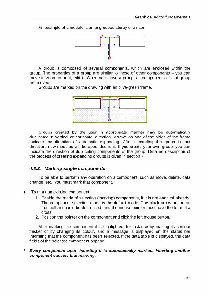
Graphical editor fundamentals
61
An example of a module is an ungrouped storey of a riser:
A group is composed of several components, which are enclosed within the
group. The properties of a group are similar to those of other components – you can move it, zoom in on it, edit it. When you move a group, all components of that group are moved.
Groups are marked on the drawing with an olive-green frame.
Groups created by the user in appropriate manner may be automatically
duplicated in vertical or horizontal direction. Arrows on one of the sides of the frame indicate the direction of automatic expanding. After expanding the group in that direction, new modules will be appended to it. If you create your own group, you can indicate the direction of duplicating components of the group. Detailed description of the process of creating expanding groups is given in section 7.
4.8.2. Marking single components
To be able to perform any operation on a component, such as move, delete, data change, etc., you must mark that component.
♦ To mark an existing component:
1. Enable the mode of selecting (marking) components, if it is not enabled already. The component selection mode is the default mode. The black arrow button on the toolbar should be depressed, and the mouse pointer must have the form of a cross.
2. Position the pointer on the component and click the left mouse button. After marking the component it is highlighted, for instance by making its contour
thicker or by changing its colour, and a message is displayed on the status bar informing that the component has been selected. If the data table is displayed, the data fields of the selected component appear.
! Every component upon inserting it is automatically marked. Inserting another
component cancels that marking.
Graphical editor fundamentals
62
! When marking a polyline clicking on one of its segments marks that segment only. To mark entire length of a polyline double click any fragment of it.
You can mark a component which is obscured by another component placed on
top of it.
♦ To mark a component obscured by another: 1. Click the component which is “on top”; this component becomes marked. 2. Press and hold the Ctrl key. 3. While keeping the Ctrl key depressed, click the component which is underneath
(within the area which is shared by the two components). 4. Release the Ctrl key. 5. The component “on top” will be unmarked and the component “underneath” will
be marked.
♦ To unmark a component click a point within the workspace where there is no component. The status line should then display “Selected: ---”. You can also use the
“Unmark all components” function ( ).
4.8.3. Marking multiple components
Most of the operations can be done not only on single components, but on groups of components. To perform an operation on multiple components, you have to mark them.
! Marking multiple components and editing them simultaneously can substantially
speed up your work. Marking multiple components is of special significance when appending data (see section 4.9.5).
There are several methods of marking multiple components in the graphical
editor. The choice of the method depends on the components that are to be marked and on their relative arrangement. Available methods of marking groups of components are described below.
♦ To unmark multiple components proceed as in the case of a single component. Click
a point within the workspace where there is no component. The status line should then
display “Selected: ---”. You can also use the “Unmark all components” function ( ).
4.8.4. Marking multiple components with the use of the Shift key
♦ To mark several components: 1. Enable the mode of selecting (marking) components, if it is not enabled already.
The component selection mode is the default mode. The black arrow button on the toolbar should be depressed, and the mouse pointer must have the form of a cross.
2. Position the pointer on one of the components and click the left mouse button to mark it.

Graphical editor fundamentals
63
3. Press and hold the Shift key. 4. While keeping the Shift key depressed, click the second and following
components. These components will be marked without unmarking the previous ones.
5. If you have marked a wrong component, click it once more (while still pressing the Shift key) and it will be unmarked.
6. Release the Shift key. 7. All the indicated components will be marked. This is indicated by changed colour
or by thicker outline. The status line displays the number of marked components. To unmark multiple components click a point within the workspace where there is
no component. The status line should then display “Selected: ---”. You can also use the
“Unmark all components” function ( ).
! You can combine the functions of the Shift and Ctrl keys (marking obscured components; function described in the previous item) when marking components.
4.8.5. Marking multiple components within a specified area
It is possible to mark all components located within a specified area. You can also restrict marking to components of a specified type. The latter feature is particularly helpful when appending data.
♦ To mark all components within a specified area:
1. Select “Edit / Select components in rectangle” (“Functions” –> ). This command is also available in the pop-up menu displayed upon clicking the right mouse button with the mouse pointer positioned within the workspace.
2. Position the mouse pointer in one corner of the area with the components to be marked and press the left mouse button.
3. While keeping the mouse button depressed, mark the required area. The area is represented by a pink rectangle.
4. The components within the selected area will be marked when you release the mouse button.
! The following rules apply to component marking within selected area:
– if you select the area from left to right, then only those components that are entirely enclosed within the selected area will be marked. The selected area is in this case drawn with a solid line – if you select the area from right to left, then all components entirely and partly enclosed within the selected area will be marked. The selected area is in this case drawn with a dashed line.
It is also possible to mark components of a specified type only (e.g. sections, etc.)
This is very helpful in appending data.

Graphical editor fundamentals
64
♦ To mark all components of a specified type within selected area:
1. Select “Edit / Select in rectangle components of type ...” (“Functions” –> ). This command is also available in the pop-up menu displayed upon clicking the right mouse button with the mouse pointer positioned within the workspace.
2. Select from the pull-down menu the required type of components to be marked. 3. Position the mouse pointer in one corner of the area with the components to be
marked and press the left mouse button. 4. While keeping the mouse button depressed, mark the area. The area is
represented by a pink rectangle. 5. The components within the selected area will be marked when you release the
mouse button.
! You can configure the menu of component types to be selected (marked).
4.8.6. Marking multiple components of specified type in the entire sheet
If you want to mark all components in the project or all components of a specified type, there are functions available similar to marking components within a specified area. These functions, however, apply to the entire sheet:
- “Edit / Select all components” (Ctrl+A).
and - “Edit / Select all components of type ...”, which display pop-up menus to select
component type to be marked.
4.8.7. Moving component
Nearly every component inserted into the project can be moved freely and placed in any location. The exceptions are components that are placed on other components, such as valves. Components of this type cannot be moved at all or they can be moved only within a specified range. A valve, for instance, can only be moved within its system section.
♦ To move a component:
1. Make sure that the mode of selecting components is enabled (the button with a black arrow on the toolbar is depressed).
2. Position the mouse pointer on the component and click and hold the left mouse button (the component is marked).
3. With the left mouse button depressed drag the component to a new position. 4. Release the mouse button (the component remains marked).
! If more than one component is marked, dragging any of them causes all the
marked components to be moved. If the GRID mode (drawing grid) is enabled when components are moved, then
the components are moved in accordance with the specified horizontal and vertical grid spacing.

Graphical editor fundamentals
65
It is also possible to move one or more selected components using cursor control keys, which is one of the ways to effect a vertical only or horizontal only movement. Pressing the Alt+<cursor control key> key combination moves the component by a distance equal to the minimum ruler interval, pressing the Alt+Shift+< cursor control key > key combination moves the component by a distance equal to 0.1 of the minimum ruler interval. In the GRID mode small movements cannot be effected. The described manner of moving components is convenient for precise positioning of components.
! A heating zone cannot be moved because it is assigned to a room. However, you
can move the box with HZ label.
4.8.8. Flipping a component horizontally
Nearly every component or module can be turned horizontally (flipped) before or after placing it in the project. The purpose of flipping a component is to change the positions of its connection points.
♦ To flip a component existing in the project (that is one that has already been inserted):
1. Mark the component(s) (see sections 4.8.3).
2. Select “Components / Flip horizontal” (Ctrl+Tab, “Functions” -> ). 3. The component is flipped:
♦ To flip a module before inserting it into the project: 1. Click on the button (icon) in the toolbar representing the module.
2. Select “Components / Flip horizontal” (Ctrl+Tab, “Functions” -> ). 3. The outline of the module is flipped: Proceed as described in section 4.8.1.
4.8.9. Changing the dimensions of components
Some components have fixed size, which cannot be changed. Other components may be modified freely by means of the mouse. Such components are, for instance, graphical components: rectangles, ellipses, etc.
All components, the size of which may be modified, have handles (black squares)
on their outlines. These handles enable expanding and contracting of the component. For instance, a rectangle may be expanded and contracted in any direction:

Graphical editor fundamentals
66
♦ To change the size of a component: 1. Make sure that the mode of selecting components is enabled (the black arrow
button on the toolbar should be depressed). 2. Position the pointer on the first component and click the left mouse button to
mark the component 3. Position the mouse pointer on one of the handles (squares). The pointer
changes shape to suggest the manner of resizing. 4. Press and hold the left mouse button. 5. While keeping the left mouse button depressed, expand or contract the
component. 6. Release the left mouse button. 7. The component takes on the modified shape.
4.8.10. Rotating a component
Some components can be rotated around its centre. Such components include, for instance, graphical components: rectangles, ellipses, etc.
All components that can be rotated have an icon , which can be grabbed and
dragged to rotate the component.
♦ To rotate a component: 1. Make sure that the mode of selecting components is (the black arrow button on
the toolbar should be depressed). 1. Position the pointer on the component and click the left mouse button to mark it. 2. Position the mouse pointer on the rotation icon . The pointer changes shape to
suggest that the component may be rotated. 3. Press and hold the left mouse button. 4. While keeping the left mouse button depressed, rotate the component. 5. Release the left mouse button.
! Pressing the Shift key when rotating a component limits the rotating capability
to several (typical) angles only: 0°, 45°, 90°.

Graphical editor fundamentals
67
4.8.11. Deleting components
The grahical editor allows simple deletion of components. If you want to delete a group of components, you can use the functions of marking groups described above and delete those components simultaneously.
♦ To delete a component from a project:
1. Mark the components you want to delete. You can use any of the methods described in sections 4.8.3 to 4.8.6.
2. Select “Edit / Delete” (Del, ).
4.8.12. Disconnecting components
Sometimes there is a need to disconnect components. This may happen, for instance, when a manifold, connection line or wall must be moved without the components attached to it.
♦ To disconnect components:
1. Click on the component.
2. Select “Components / Disconnect” (Ctrl+R, ).
4.8.13. Repeated inserting of an identical component
By default, after placing a component or module, the basic operating mode of marking and moving is restored. Often, however, you will want to insert several components of the same type. In these cases it is convenient to use the “Insert last item” command, which is assigned to the F3 function key.
♦ To place another component or module of the same type after inserting the first one,
select “Edit / Insert last item” (F3, ).
When inserting several identical components in sequence it is also possible to use the REP mode – repetitive insertion of components. When this mode is activated, components of the selected type are inserted until the right mouse button is pressed (after inserting a component, the mode of inserting that component is still activated). When REP mode is disabled, after inserting a component the mode of selecting components is activated.
The REP mode applies to structural, installation and fitting components (walls, windows, doors, radiator, heating floor, manifold, etc.).
♦ To enable or disable the REP mode:
- Click once on the REP field in the upper right corner of the screen. or
- Press the Alt+B keys.

Graphical editor fundamentals
68
! The setting described above may be helpful when editing building structure with the use of “wall” components.
4.9. Appending component data
4.9.1. Data appending fundamentals
Most of the components on which the program operates have defined data or parameters. The data table is used to edit these data.
♦ To switch the data table on / off select “View / Show / Hide data table” (F12, ) The left-hand column of the data table shows the names of the fields, while the
right-hand column displays the values. Fields assigned to fittings additionally include symbols indicating whether these data fields are displayed ( ) or hidden ( ). In the program settings you can indicate whether the fields assigned to fittings are to be displayed by default or not, meaning that groups in the data table can be represented as closed or open (see section 7.3.1).
! Some of the fields have hints assigned to them, which appear on the screen
when you position the mouse pointer on the field (without pressing the mouse keys).
The contents of the data table varies, and the fields that appear in the table
depend on the component marked. If several components of the same type have been selected, the table contains fields common to all marked components. If components of different types have been marked, the data table will not contain any fields.
! Marking many components of the same type and editing them simultaneously
may speed up data appending substantially (see section 4.9.7).
! To append data you have to mark (select) components. To avoid unintended displacement of components, it is advisable to lock them (LOCK mode) before starting data appending (see section 4.6.2).
4.9.2. Data table field types and editing
The data table may consist of fields of various types. The field type determines the manner of editing it. Many data and values are determined automatically on the basis of the drawing or other data. These values are shown enclosed in brackets and the user can overwrite them.
! To restore the default value (assigned by the program) enter “?” in the given
field and press the “Enter” key. The data table can include the following types of fields (examples are provided for
graphical components): 1. Text fields.

Graphical editor fundamentals
69
2. Numerical fields. 3. Selection fields (multiple option fields, with an arrow next to the field name). 4. Compound fields (name followed by dots ...). 5. Information fields.
! Data tables may also include fields of mixed nature.
1. Text fields In the text field you can enter text. In some cases the number of characters that
can be entered is limited. To confirm the new contents of the text field you have just entered, press the Enter key.
An example of a text field is “Text” for a rectangle. 2. Numerical fields Numerical fields enable you to enter numerical values. The value that is entered
into a numerical field is usually checked automatically to see whether it is within specified range. If an out-of-range value is entered, then an audible warning signal is issued and the lowest or highest value within the permissible range is adopted, depending on the entered value being too low or too high. To confirm the new value in the numerical field press the Enter key.
In some numerical fields it is possible to enter special values, represented by letters or other characters. Special values are always explained in field hints. An example of a numerical field is “Height [mm]” for a rectangle.
3. Selection fields In the case of some fields the range of values that can be entered is limited (e.g.
“Arrow type” indicating arrowhead type at the starting point and at the end of a polyline). After clicking on a field of this type an additional button appears on the right side of the field which enables displaying a list of available values. Clicking on this button expands the list:
! When entering data, instead of using the mouse to display the list of values, you can press the Ctrl + Enter key combination. Ctrl + Enter is also used to close the list.

Graphical editor fundamentals
70
To complete editing the field, after indicating the proper option, you can click on the arrow on the right side of the field or click on another field in the data table. Double clicking on the selected option also closes the list.
! Double clicking on a selection field selects the following option in the list.
The lists that are displayed in the data table may be single-level or multilevel lists.
In the multilevel lists sub-options are represented by yellow folders. To expand or contract a group, double click on it or position the mouse pointer on it and press the Enter key.
4. Compound fields Some fields require that more than one value is specified. In this case compound
fields are used. When you click on a compound field, a button with an arrow or three dots (ellipsis) appears on the right side of the field, similar to the one in selection fields. Clicking on this button opens an additional box with various fields, depending on the needs. An example of a compound field is the “Font” field.
You can close the window after specifying the values in the fields. To open or
close a compound field, as was the case with selection fields, you can use the Ctrl+Enter keys. Editing can also be completed by clicking on the arrow on the right side of the field or by clicking on another field in the data table.
5. Information fields Some fields serve only the purpose of informing and the user cannot modify them.
After clicking on a field of this type a narrow coloured outline appears around it.
4.9.3. Specifying types. Letter shortcuts
Pipe type and valve type fields are selection fields. In each of these fields you can display a list of available types. You can select any type of pipe from any catalogue you like.
! List of types displayed in the data table depends on the catalogues selected in
the project.
! Connection type and fittings can be specified only after the pipe type is specified.
In the current version of the software you can assign letters to fittings and
components from catalogues: pipes and pipe fittings, valves and fittings, insulation, radiators and radiant heating components. The types and fittings used most often may then have their letter shortcuts assigned to facilitate design work.
Of course, you can always choose any required component from a list without assigning a letter shortcut.

Graphical editor fundamentals
71
♦ To assign a letter shortcut:
1. Select “Options / Edit letter shortcuts” (Ctrl+L ). 2. Enter in the “New shortcut” field a letter or a sequence of letters which is to form
the assigned shortcut. No distinction is made between lower and upper case letters.
3. Choose the component you want to assign the letter shortcut to in the “Catalogue item” list.
4. Click the “Assign” button. 5. Click “OK” to carry the assignment into effect.
♦ To delete a letter shortcut:
1. Select “Options / Edit letter shortcuts” (Ctrl+L ). 2. Select in the “Defined shortcuts” list the shortcut you want to delete and
component assigned to it. 3. Click the “Delete” button. 4. Click “OK” to carry the deletion into effect.
♦ To display the list of current letter shortcuts select View / Show/hide letter shortcuts
.
A letter shortcut applies to a family of pipes or a family of other components. This
means that when in the data table you enter a letter assigned to a pipe type in the “Pipe type” field, the program will select pipe type size from the chosen pipe family. To impose pipe diameter, enter: <diameter> <letter shortcut>, e.g. 10a, if a pipe type is assigned to “a”.
Graphical editor fundamentals
72
Remember that letter shortcuts are assigned to user, not to the project, and that means that, for instance, they cannot be transferred with the project file onto another computer.
4.9.4. Local resistance components
Local resistance components in the application can be divided into those which are displayed and those which are not. All displayed local resistance components have their data in separate fields of data table. Local resistance components, which are not displayed, are entered in the “Miscellaneous components” field.
! For each pipe-run you can enter various “miscellaneous components”, which
are compatible with the pipe type of the pipe-run. Therefore, to be able to enter local resistance components from a pipe catalogue, first you have to specify the pipe type.
Local resistance components may be entered into the “Miscellaneous
components” field by means of letter shortcuts or by selecting from a list. After clicking the button on the right side of the field, a special window appears, where you can specify local resistance components on the marked pipe-run (or pipe-runs, if more than one is marked).
A list of available resistance components is in the left part of the window. The list
on the right side includes the selected local resistance components. You can move items from one list to the other using the buttons with arrows placed between the two lists. The number in brackets at the end of component name in the list on the right indicates the number of selected components of that type.
The top of the list of available resistance components includes pipe fittings from
the pipe catalogue. Next come the components from local resistance component catalogue that can be installed on any type of pipe. Successive items include components with specified Kv, zeta or pressure drop (in kPa). Macrodefinitions are at the end of the list. The values of Kv, zeta or pressure drop are input in a field below the list of selected components.
! The list of available resistance components includes those macrodefinitions,
which are compatible with the selected pipe type. You can enter local resistance components without opening the window described
above. This, however, applies only to those components that have letter shortcuts assigned. For instance, if letter “b” is assigned to a 90º bend, then you can just enter b in the “Miscellaneous components” field to specify one bend, or bbb to specify three bends.
To add a macrodefinition to the list of local resistance components, enter
*<number> (e.g. *1). You can also enter components with zeta value specified in square brackets, e.g. [5.2], Kv value in round brackets, e.g. (5.2) or pressure drop in kilopascals in braces, e.g. {1,2}.

Graphical editor fundamentals
73
4.9.5. Repeated entering of the same data
Often many components in a project have the same data. If this is the case, to speed up editing, you can apply one of the methods, which facilitate repeated entering of the same data:
- Repeat the last value. - Enter data simultaneously for multiple components. - Sets of typical values.
These methods are described in the subsections that follow.
4.9.6. Repeating the last value
This is the simplest method of duplicating component data. After specifying data for one component and marking the following component you don’t have to enter the data once more, just make use of the repeat feature.
♦ To enter data by repeating last value:
1. Mark one component. 2. Enter data. 3. Mark next component – the same field should be indicated in the table. 4. Select “Component data / Repeat last value” (F2).
! Last values are stored for 10 data fields.
If no last value is stored for the field selected, this is indicated by an audible
warning signal and an appropriate message in the status bar.
4.9.7. Simultaneous entering of data for multiple components
This is the second fast method of entering data for multiple components. After marking several components, fields common to all these components are displayed in the data table. The values in the fields that are identical for all marked components are displayed in the table; other fields are empty.
If you enter a value in any of these fields, that value becomes valid for all marked components, no matter whether the values for individual components before entering the new value were identical or different. The fields that are not edited will not change their contents.
♦ To change a value for multiple components simultaneously:
1. Mark the components. You can use all the techniques described in section 4.8.3 to 4.8.6.
2. Enter data in appropriate fields in the data table.

Graphical editor fundamentals
74
4.9.8. Data sets and data sets gallery
In this method selected component data are stored in the form of a set and then the set is pasted into other components. The stored data sets form the contents of the data sets list, which can be used during further editing.
♦ To save a data set:
1. Mark the component and append its data (if not appended before). 2. Click the right mouse button with the pointer positioned within the data table or
click the scroll button of the pop-up menu in the data table: . 3. Select “Save as data set” in the pop-up menu. 4. A list of fields to be saved in the set appears (initially the list is empty). 5. Using the arrow buttons, move the fields to be saved in the data set. To do this
select the field or several fields using the Shift or Ctrl key and click the appropriate button. A single arrow moves only the marked fields, double arrow moves all fields.
6. Click “OK” to save the data set or “Cancel” to abandon. An example of a data set creation window is shown below:
The created data sets are displayed in a special window of the data sets list.
♦ To switch a data sets list on or off select ”View / Show/Hide data sets list” (F9, ) The list presents the stored data sets in the following form: <field_value> (<field_name>); <field_value> (<field_name >); [...]
for example:
! When you position the mouse pointer on a data set, a hint is displayed showing which fields are stored in the set.
Data sets may be used for individual components or multiple marked components.

Graphical editor fundamentals
75
♦ To paste a data set into individual components one by one: 1. Switch on the data sets list (if it is not displayed yet). 2. Click on the selected data set within the data sets list. The shape of the mouse
pointer changes into an arrow with a data table attached. 3. Click the left mouse button on all the components which are to take on the field
values of the selected data set. 4. Click the right mouse button to complete the “pasting” of data sets.
♦ To paste a data set into many components at once:
1. Switch on the data sets list (if it is not displayed yet). 2. Mark the components which are to take on the data from the data set. You can
use all the techniques described in sections 4.8.3 to 4.8.6. 3. Double click on the data set in the data sets list. 4. The data set is “pasted” into all marked components.
Data sets gallery You can process the saved data sets: delete them, change their descriptions, etc.
The data sets gallery is designed for this purpose.
♦ To switch a data sets gallery on select “Component data / Data sets gallery...” The data sets gallery window is presented below:
The main part of the window is the list of data sets. Data sets are presented in the
same manner as in the data sets list, the only difference being letter “L”, which may appear beside some of the data sets. This symbol indicates that the data set will be saved to a user library and not to the project file. It will then be possible to use that data set in all your projects. Data sets that are not marked with the “L” symbol are saved to the project file.
When you click on a data set, its contents are shown on the right side of the
window. A checkbox under the list of sets is used to specify whether the selected data set is to be saved to a user library or not. In the “Label” field you can change the description of the selected data set. The “Delete” button enables you to remove the data set from the list.

Graphical editor fundamentals
76
4.9.9. Moving between components using the keyboard
The mouse is a convenient tool for editing drawings. However, when you want to edit component data, you need the keyboard. To avoid repeated shifting of your hand from the keyboard to the mouse and back, you can use the keyboard to move from one component to another.
The graphical editor features two modes of moving between components by means of the keyboard:
- moving to the nearest component in specified direction - moving to the next connected component in specified direction.
Moving to the nearest component in specified direction:
This mode is most convenient for moving between components of the same type
within a project.
♦ To move to the nearest component by means of the keyboard: 1. Mark one of the components. Its data is shown in the data table. To move about
between the data in the table, use the cursor control keys: - Press Ctrl+<cursor control key> to move in the direction indicated by the
cursor control key to the nearest component of the same type (e.g. from a middle section of a profile to the next or preceding middle section)
- Press Ctrl+Alt+<cursor control key> to move in the direction indicated by the cursor control key to the nearest component of other type (e.g. from a middle section of a profile to the starting point of the profile).
<cursor control key> indicates one of the keys in the cursor control keypad.
! The movement is made to the component that is nearest in geometrical terms.
Sometimes this may not be what the user expects.
After shifting to another component of the same type, its data are shown in the data table, which you can alter. The current field in the data table is not changed. This enables fast entering of data in one field. You can also use the function of repeating the last value (see section 4.9.6).
If the value is the same for all components, it is better to use one of the methods of marking multiple components (see section 4.8.3).
Moving to the next connected component in specified direction:
This mode is most convenient for moving between segments of a system within a
project.
♦ To move to the next connected component in specified direction: 1. Mark one of the components. Its data is shown in the data table. To move about
between the data in the table, use the cursor control keys.

Graphical editor fundamentals
77
2. Make sure that the Num Lock mode of the keyboard is enabled – relevant LED is on.
3. Press Ctrl+< key of the numeric keypad >. The direction of movement is determined by the position of the key in relation to key 5, and accordingly: key 8 – move to the component connected “at the top” of the selected component, key 9 - component connected “at the top and to the right” of the selected component, key 6 – “to the right”, key 3 – “down, to the right”, etc. The diagram below illustrates this:
ã 7
8 á
9 ä
ß 4 5 6
à å 1
2 â
3 æ
! The keyboard can only be used to move from one component to another to
append their data. To move or enter new components you have to use the mouse.
4.10. Hardware and fittings
4.10.1. Basic information
Besides the main components, which make up the structure of the installation in Instal-therm, there are many additional components, such as valves or gates, protecting tubes, etc. They all have been given a collective name of “hardware and fittings”. Their characteristic and common feature is that they are placed on other, existing components in the project.
! Hardware or fitting is a component that cannot stand alone in the project, it must
be assigned to other component. ! Graphical components, such as pipe-run labels, have similar properties. All
operations that can be executed on fitting components can also be done on pipe-run labels.
Description of the various hardware and fitting components is given in the
following sections of the manual.
4.10.2. Inserting single fitting components
Fitting components are placed in a similar manner to ordinary components. The difference is that a fitting component must be inserted to an existing component, which we named basic component (for instance pipe-runs).

Graphical editor fundamentals
78
♦ To insert a fitting component: 1. Make sure that the basic component, onto which fittings will be added, already
exists in the project. 1. Click the button representing the required fitting component. 2. As you move the mouse within the project, the outline of the selected component
is displayed. 3. Click the basic component into which you want to insert the fitting. The fitting will
be inserted only if the fitting component is logically compatible with the basic component.
4. Depending on the set mode of inserting fittings, the component-marking mode is enabled or insertion of another identical fitting is proposed. In the latter case, if you want to abandon inserting fittings, press the right mouse button. Configuration of the mode of inserting fittings is described in section 7.3.1.
! Always click on the component (fragment of the system under design), onto
which you want to install the fitting.
! This is of particular importance when a radiator coupling is inserted, which in the drawing is beside the radiator. Logically it forms part of the radiator and space for drawing the radiator coupling will be located automatically. The sequence will look like this:
During inserting After insertion
4.10.3. Deleting fitting components
To delete a fitting or hardware component you first have to select (mark) it. Therefore, when selecting fitting or hardware components for deletion, always observe messages in the status line to be sure not to select and delete the basic component on which the fitting or hardware is placed.
Remember, that when you delete a basic component that includes fittings, those
fittings will also be deleted. You can always undo a delete operation (see section 4.7).
4.10.4. Inserting multiple fittings
The graphical editor enables fast insertion of many identical fittings into existing basic components in a project.
♦ To insert fittings into many basic components fast:
1. Mark the basic components into which you want to insert the fittings. You can use all the techniques described in sections 4.8.3 to 4.8.6.

Graphical editor fundamentals
79
2. Double click the toolbar button representing the required fitting component. Fittings are inserted into all marked components, provided that the component type is logically compatible with the basic components.
4.10.5. Appending fitting component data
As mentioned, fittings are not independent components. They must always be assigned to other components. Fitting component data are also appended in the data table. When you click on the fitting or the corresponding basic component, the data table displays data of the main component at the top, and the data of the fitting beneath:
These data always begin with the name of the selected hardware or fitting
component followed by fields of the selected fitting. These fields are marked with “•”. First field of each fitting is marked with a white symbol or . The symbol
indicates that the remaining fields of that component are contracted (hidden). The symbol indicates that the remaining fields of that component are displayed. To hide or display the fields click on or .
Data of some fitting components consist of only one field. Some other components have no fields in the data table at all.
4.10.6. Selecting the manner of drawing fitting components
Some fitting components may be represented by various graphical symbols and most of them can be flipped vertically or horizontally.
The manner of drawing a fitting is represented by one of the fields in the data
table. By changing the value of that field you can select the drawing of the fitting. For instance, when you insert a pressure gauge, a “Pressure gauge ...” field appears, where you can select an item from a list. The list contains graphical representations of the pressure gauge:
Graphic
al symb

Graphical editor fundamentals
80
ol
Value in the “Pressure gauge
...” field
Standard, w/o valve
Standard, with valve Natural
Flipping components vertically and horizontally may be done in two ways: using
the mouse in the drawing or in the data table. Upon clicking on a fitting, which can be flipped vertically or horizontally, a green
symbol with an arrow appears. This symbol is used to flip the component. Below a valve is shown as an example:
By dragging the dot with the mouse you can flip the valve vertically or horizontally.
In the case of a straight-run valve, flipping it horizontally changes only the direction of valve label, while in the case of an angle valve the orientation of the valve is also changed.
A similar operation can be performed in the data table. When you click on the
button to the right of the “• Rotate dwg.” field, a window is displayed that enables “horizontal” (Inverted x) or “vertical” flipping of valve. Remember that “horizontal” means here the direction parallel to the valve axis, whereas “vertical” means perpendicular to the valve axis.
In the described window there is also a “Maintain vertical” box. If pipe-run inclinations are accounted for in the drawing and the valves are to be drawn upright (not perpendicular to pipe-run), then the “Maintain vertical” box should be checked:
“Maintain vertical” box
unchecked “Maintain vertical” box
checked You can also change the position of the valve label. When you click on a valve, a
yellow frame appears. You can drag this frame with the mouse to the location you require.
Valve label can also be relocated using the “Label pos.” field in the data table. You can also choose one of the predefined valve labels.
! Flipping the valves and moving their labels with the use of the appropriate fields in the data table is convenient when this operation must be carried out on many valves at once.

Graphical editor fundamentals
81
♦ To flip many valves or move their labels: 1. Mark the pipe-runs with the valves. 2. Pipe-run fields with valve fields appear in the data table. 3. Open the window for flipping the valve (“Rotate dwg.”) or the field for moving
the label (“Label pos.”) and perform the required operation. The operation is carried out on all marked components.
4.11. Inserting and configuring pipe-run labels
Pipe-run labels are components that, like fittings, are placed on pipe-runs (system segments), in order to permanently display basic calculation results (such as pipe diameter and type) on the drawing. Buttons representing pipe-run labels are on the toolbar in the “Graphics” tab:
– oblique pipe-run label – enables setting of any position of reference line and text and rotation through 90°.
– level pipe-run label – reference line is perpendicular to pipe-run drawing and text is placed over and under the line.
– simplified pipe-run label – text is placed directly above pipe-run drawing. Reference lines are not drawn.
Inserting pipe-run labels is done the same way as inserting fittings. Fast methods
of inserting pipe-run labels, described in section 4.10.4, can also be applied.
♦ You can rotate oblique and level pipe-run labels using the mouse. To rotate pipe-run label:
1. Mark the pipe-run label. At the end of the reference line a small icon appears. 2. Position the mouse pointer on . Press and hold the left mouse button. 3. Keep the mouse button depressed and rotate the label. 4. Release the mouse button.
♦ In an oblique label you can additionally change the position of the reference line. To
move the reference line: 1. Position the mouse pointer on the horizontal part of the reference line. Press and
hold the left mouse button. 2. Keep the mouse button depressed and move the reference line to the required
location. 3. Release the mouse button.
After placing the pipe-run label, data for configuring the label appear in the data
table:
Pipe-run label:

Graphical editor fundamentals
82
Complex field. Provide indicating data and results you want to place above the line, under the line or beside the line.
Rotate dwg.:
Complex field. Provide rotating pipe-run label. Used mainly when configuring many pipe-run labels.
A configured label placed on a pipe-run may be saved to the toolbar provided for
user-defined modules.
♦ To save a pipe-run label and its settings, mark that label on the drawing and select “Modules / Append to toolbar” in the menu. The modules gallery window appears where you can add your label to a new component. After clicking OK., the new pipe-run label becomes available on the user-defined modules tab.
4.12. Connection points
Connections between components are made already at the stage of creating the layout of the system. Component connection points are shown in the form of squares.
An unconnected point is represented by an empty square:
Connected points are represented by smaller filled squares: . This system of presenting connections facilitates fast spotting out of unconnected
components (also in small scale) and correcting connections before starting calculations.
! You must remember that no more than 4 pipe-runs may be connected in one
point. Fifth connection cannot be executed and this is indicated on the diagram:
! Pipe-runs may consist of several segments. To differentiate between connection points of two pipe-runs and internal nodes within a pipe-run, the latter are represented by diamonds:

Components of the base building drawing
83
5. COMPONENTS OF THE BASE BUILDING DRAWING
5.1. Introduction
The base building drawing may consists of: - plan view sheets with the building structure displayed (walls, rooms, etc.) - schematic view sheets with the cross section of the floors.
! The arrangement of rooms is not represented in the schematic views.
The graphical editor enables drawing plan views of individual storeys of the
building for which the system is designed and/or for which we want to do heat loss calculations. The plan view of a storey is the indispensable basis for radiant heating design.
It is possible to import a plan view from a file created with other software application, e,g, a CAD application. A DXF/DWG file may be imported with the drawing interpreted or not. Both operations are described in section 7.
The most prominent feature of the algorithm of loading DWG/DXF is the possibility of interpreting them, i.e. identifying and inserting into the project walls, windows and doors as program objects (equivalent to those inserted manually) and identifying the structure of rooms on a storey. The efficiency of identifying the structure of rooms depends heavily on the understanding of the structure of layers in the file and on care taken to make the drawing in the graphical application. Several rooms, for instance, may be combined into one when no door is inserted in the wall in the drawing (or if such door actually does not exist). In such or similar cases there are various ways of imposing a room structure in the drawing, which is discussed further in this manual.
! Horizontal partitions – floors on ground, roofs and floors – are not created
during import. These should be inserted manually in the graphical editor (in the form of graphical partitions) or in tables in Instal-heat&energy (as tabular partitions).
The program enables loading any drawing (e.g. in EMF/WMF or BMP format, and
also in DWG and DXF format – without interpreting), which may form a background for drawing the structure of a storey using components available in the program.
5.2. Components of a storey plan view
Components that make up the plan view of the building saved to the “Plan view” sheet in the “Construction” layer are described below in detail. The properties and data apply to objects both drawn in the program and imported from a DWG or DXF file and interpreted. During import, however, only objects such as “Wall”, “Window”, “Door” and “Room” can be formed. Each component has a button for inserting assigned in the toolbar and a detailed description of component data fields.

Components of the base building drawing
84
5.2.1. Wall
The “Wall” component is used to enclose rooms. A rule has been adopted that a single wall is a straight segment. If you want to insert an angled wall, you have to make it up of several “Wall” type components.
Button on the “Components” toolbar: Appearance on screen:
“Wall” component data:
Length within axes [m] Numerical field. Length of wall within axes. This field may be filled when inserting a wall (after marking one end of the wall). Then the entered length is retained in the drawing. A value in brackets indicates length read from the drawing. Angle Numerical field. Angle in relation to the X-axis. This field may be filled when inserting a wall. Then the entered length is retained in the drawing. A value in brackets indicates angle read from the drawing. Thickness [m] Numerical field. Thickness of the wall. This field may be filled when inserting the wall. When you click on the field, an arrow appears on the right side of the field which opens a window for editing the thicknesses of the “right” and “left” side of the wall. Thus you can create an asymmetrical wall. In this case the broken line inside the wall is no longer the axis of that wall. Partition structure type Selection field. When specification of partitions is done in Instal-heat&energy, and partitions have already been defined there, then this is a selection field where you can select a pre-defined partition from a list. If a type has already been assigned to the wall in Instal-heat&energy, then its name is automatically displayed in the graphical editor and the appropriate U0 coefficient is displayed in the field below. U0 / UN / R Numerical field. Coefficient of heat transfer across partition / thermal resistance of partition. When specification of partitions is done in Instal-heat&energy, then this field cannot be modified. It is automatically filled in for the partition type selected from list. The name of partition structure and U0 coefficient can be entered directly from the keyboard in the graphical editor – then after loading the project into Instal-heat&energy, the partition type and U0 assigned to the given partition in the room are displayed in the building structure.

Components of the base building drawing
85
Height within axes [m] Numerical field. Height of wall within its axes. Value taken from storey data of the building structure. Area within axes [m2] Numerical field. Wall surface area within its axes. Value in brackets indicates area calculated from data in the drawing. Length within faces [m] Numerical field. Length of wall within its faces. Cannot be modified. Value in brackets indicates length read from the drawing. Height within faces [m] Numerical field. Height of wall within its faces. Value taken from storey data of the building structure. Area within faces [m2] Numerical field. Wall surface area within its faces. Value in brackets indicates area calculated from data in the drawing. Outer length [m] Numerical field. Length of wall in external dimensions. Cannot be modified. Value in brackets indicates length read from the drawing. Outer height [m] Numerical field. Height of wall in external dimensions. Outer area [m2] Numerical field. Surface area of wall in external dimensions. Value in brackets indicates area calculated from data in the drawing. Calculated in Instal-heat&energy Selection field. Determines whether partition is to be accounted for in Instal-heat&energy during heat loss calculations. Wall type Selection field. The available entries are “External” and ”Internal”. The type of wall is important when placing heating zones in the rooms. The strip of non-heated floor along the wall is taken into account, and the width of that strip depends on the type of wall. The spacing for external and internal walls is specified in “Options / General data” (F7). Spacing between HZ and wall [m] Numerical field. Distance between heating zone and wall. Value in brackets indicates a value entered automatically depending on the type of wall. You may enter a non-standard value of the spacing.
5.2.2. Curved wall
The “Curved wall” component is used to edit rooms of specific shape.
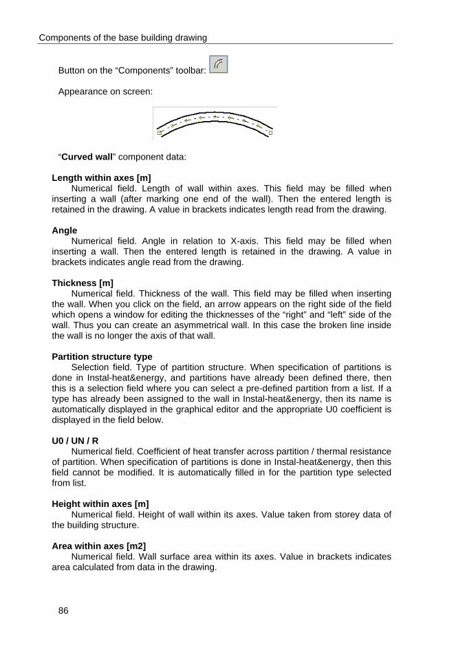
Components of the base building drawing
86
Button on the “Components” toolbar: Appearance on screen:
“Curved wall” component data:
Length within axes [m] Numerical field. Length of wall within axes. This field may be filled when inserting a wall (after marking one end of the wall). Then the entered length is retained in the drawing. A value in brackets indicates length read from the drawing. Angle Numerical field. Angle in relation to X-axis. This field may be filled when inserting a wall. Then the entered length is retained in the drawing. A value in brackets indicates angle read from the drawing. Thickness [m] Numerical field. Thickness of the wall. This field may be filled when inserting the wall. When you click on the field, an arrow appears on the right side of the field which opens a window for editing the thicknesses of the “right” and “left” side of the wall. Thus you can create an asymmetrical wall. In this case the broken line inside the wall is no longer the axis of that wall. Partition structure type Selection field. Type of partition structure. When specification of partitions is done in Instal-heat&energy, and partitions have already been defined there, then this is a selection field where you can select a pre-defined partition from a list. If a type has already been assigned to the wall in Instal-heat&energy, then its name is automatically displayed in the graphical editor and the appropriate U0 coefficient is displayed in the field below. U0 / UN / R Numerical field. Coefficient of heat transfer across partition / thermal resistance of partition. When specification of partitions is done in Instal-heat&energy, then this field cannot be modified. It is automatically filled in for the partition type selected from list. Height within axes [m] Numerical field. Height of wall within its axes. Value taken from storey data of the building structure. Area within axes [m2] Numerical field. Wall surface area within its axes. Value in brackets indicates area calculated from data in the drawing.

Components of the base building drawing
87
Length within faces [m] Numerical field. Length of wall within its faces. Cannot be modified. Value in brackets indicates length read from the drawing. Height within faces [m] Numerical field. Height of wall within its faces. Value taken from storey data of the building structure. Area within faces [m2] Numerical field. Wall surface area within its faces. Value in brackets indicates area calculated from data in the drawing. Outer length [m] Numerical field. Length of wall in external dimensions. Cannot be modified. Value in brackets indicates length read from the drawing. Outer height [m] Numerical field. Height of wall in external dimensions. Default value is equal to the height within axes. Outer area [m2] Numerical field. Surface area of wall in external dimensions. Value in brackets indicates area calculated from data in the drawing. Calculated in Instal-heat&energy Selection field. Determines whether partition is to be accounted for in Instal-heat&energy during heat loss calculations. Wall type Selection field. The available entries are “External” and ”Internal”. The type of wall is important when placing heating zones in the rooms. The strip of non-heated floor along the wall is taken into account, and the width of that strip depends on the type of wall. The spacing for external and internal walls is specified in “Options / General data” (F7). No. of arc segments Numerical field. Number of segments of polyline used to draw the curved wall. Value in brackets indicates the value determined automatically from the maximum angle of inflection. You may specify other value – then the value is adapted to the number given. Spacing between HZ and wall Numerical field. Distance between heating zone and wall. Value in brackets indicates a value entered automatically depending on the type of wall. You may enter a non-standard value of the spacing.
5.2.3. Opening in wall
The “Opening in wall” component cannot stand alone – it may only be placed on a wall to which it is assigned, and its data are displayed in the lower part of the wall data table. This is a graphical component and has no effect on calculations, in particular it

Components of the base building drawing
88
does not eliminate partitioning of rooms by walls. To place an opening in a wall, select it from the “Components” toolbar and click on the wall axis at a selected point. You can move the opening along the wall.
Button on the “Components” toolbar: Appearance on screen:
“Opening in wall” component data:
Width [m] Numerical field. Width of opening along the axis of the wall. Height [m] Numerical field. Height of opening. Draw line Selection field. This field can be set to “Yes” or “No” and it applies to the manner of drawing. The “Yes” setting means that wall contour is drawn along opening
5.2.4. Window
The “Window” component cannot stand alone – it may only be placed on a wall to which it is assigned, and its data is displayed in the lower part of the wall data table. It is taken into account when heat loss calculations are done in Instal-heat&energy – just like in the case of a wall, the window has a partition structure assigned, and the surface area of the window is subtracted from the calculated surface area of the wall in which the window is installed. This component is displayed in Instal-heat&energy tables as the so-called subpartition, i.e. a nested partition (subordinate to parent partition – the wall). This ensures that the net surface area of the parent partition is always updated, without the need to subtract area or U coefficients of these partitions.
Radiators inserted into the project in the AUTO mode are automatically aligned
with the middle of the window. To place a window in a wall, select it from the “Components” toolbar and click on
the wall axis at a selected point. You can move the window along the wall or reorient it by dragging to the opposite side of the wall the square with arrow displayed after marking the window.
Button on the “Components” toolbar:

Components of the base building drawing
89
Appearance on screen:
“Window” component data:
Width [m] Numerical field. Width of the window in metres measured along the wall axis. The default value is taken from data of the building structure. If this value is not specified there, then the width of window inserted into the drawing is 0.8 m. Thickness [m] Numerical field. Thickness of the window. Has effect on the location of contraction on the drawing. Height [m] Numerical field. Height of the window.
Drawing type Selection field. Drawing type that determines whether the window is drawn as a single window with or without a frame or a double window. You can make your selection from a list of available types.
Partition structure type Selection field. Type of partition structure. When heat loss calculations for rooms and specification of partitions is done in Instal-heat&energy, then this is a selection field where you can select a pre-defined partition from a list. If a type has already been assigned to the window in Instal-heat&energy, then its name is automatically displayed in the graphical editor and the appropriate U0 coefficient is displayed in the field below. U0 Numerical field. Coefficient of heat transfer across partition. When heat loss calculations for rooms and specification of partitions is done in Instal-heat&energy, then this field cannot be modified. It is automatically filled in for the partition type selected from list.
5.2.5. Door
The “Door” component cannot stand alone – it may only be placed on a wall to which it is assigned, and its data is displayed in the lower part of the wall data table. It is taken into account when heat loss calculations are done in Instal-heat&energy – just like in the case of a wall and window, the door has a partition structure assigned, and the surface area of the door is subtracted from the calculated surface area of the wall in which the door is installed.
To place a door in a wall, select it from the “Components” toolbar and click on the wall axis at a selected point. You can move the door along the wall or reorient it by dragging the square with arrow displayed after marking the door.

Components of the base building drawing
90
Button on the “Components” toolbar: Appearance on screen:
“Door” component data:
Width [m] Numerical field. Width of the door, measured along wall axis. Height [m] Numerical field. Height of the door. Drawing type Selection field. Drawing type that determines whether the door is to be drawn as a single-leaf door (single) or a double-leaf door (double). You can make your selection from a list of available door appearance on the plan view of storey.
Partition structure type Selection field. Type of partition structure. When heat loss calculations for rooms and specification of partitions is done in Instal-heat&energy, then this is a selection field where you can select a pre-defined partition from a list. If a type has already been assigned to the door in Instal-heat&energy, then its name is automatically displayed in the graphical editor and the appropriate U0 coefficient is displayed in the field below. U0 Numerical field. Coefficient of heat transfer across partition. When heat loss calculations for rooms and specification of partitions is done in Instal-heat&energy, then this field cannot be modified. It is automatically filled in for the partition type selected from list.
5.2.6. Room
There are two types of graphical rooms in the program. One is a room formed as an enclosed space defined by walls – when such a space is created, the new object (room) is automatically identified. Another type of graphical room is a component selected from the toolbar and drawn as a polygon - room outline. In this case the room is subject to calculations in Instal-heat&energy, but all walls, windows and doors must be specified in data tables – they are not associated as drawings with the graphical editor.
! It is advisable to have only one type of rooms in one project.

Components of the base building drawing
91
Room is the key component at the stage of editing a radiant heating system: a heating zone can only be placed inside a room. Both types of rooms have the same data in the table. Room data are important during calculations, due attention must therefore be paid to them.
Button on the “Components” toolbar: Appearance on screen:
room formed by walls room from toolbar
“Room” component data:
Room symbol Text field. Symbol of a room is of descriptive nature and is designed to identify it during editing and in the tables of results. Description Text field. Description of the room. ti/θi [ºC] Numerical field. Temperature inside the room. The default value is specified in general data of the project. ti/θi below [ºC Numerical field. Temperature below used when designing floor heating system. When you enter a value here, then respective fields in HZ data of the room will not be modifiable – the value specified here is transferred to HZ data. If you enter “-“ in the “ti/θi below” field, then no temperature will be assigned and you will be able to specify different temperature for each HZ in the room. Q/Φ Numerical field. As calculations require heat loss value reduced by part of loss to heated floor or wall, this value has no significance for calculations and is included for information purposes only. You may leave this field empty. If heat loss calculations are done in Instal-heat&energy, then the calculated value appears in the data table. Qreq/Φreq. Complex field. The required output of terminal units in the room. It is equal to Q/Φ reduced (heat demand in room reduced by loss to heated floor or wall) plus the heat demand distributed from other rooms, for which heat loss distribution to other rooms has been specified. The total output of radiator, radiant heating and of other heat sources, if any, should be equal to this value. This field must be filled in.

Components of the base building drawing
92
An arrow to the right of the field enables opening Qreq//Φreq. edit window. Here you can indicate whether the heat loss in the room should be calculated in Instal-heat&energy. You can also specify the data on the type of heating systems in the room and their share in heat loss and specify the distribution of heat in the room.
RH contribution [%] Numerical field. Percentage of required output of terminal units (Qreq/Φreq.) in the entire room covered by radiant heating. The default setting is (auto). In this case, if there is both radiant and radiator heating in the room, as much heat demand as possible is covered by RH, the remainder is accounted for by sizing radiators. You can specify other value. Qrh/Φrh Numerical field. Required output of radiant heating in the room calculated on the basis of Qreq/Φreq. and RH contribution. This is the starting point for sizing. You can specify a value – contribution of RH will then be recalculated. Rad. contr. [%] Numerical field. Percentage of required output of terminal units (Qreq/Φreq.) in the entire room covered by radiator heating. The default setting is (auto). In this case, if there is both radiant and radiator heating in the room, as much heat demand as possible is covered by RH, the remainder is accounted for by sizing radiators. You can specify other value. Qrad/Φrad Numerical field. Required output of radiator heating in the room calculated on the basis of Qreq/Φreq. and rad. contr. This is the starting point for sizing. You can specify a value – rad. contr. will then be recalculated. Area w.f. Numerical field. Surface area of room within wall faces. Value in brackets indicates surface area taken from the drawing. You can overwrite that value. To revert to the value taken from the drawing, enter “?” and press Enter. Area w.a. Numerical field. Surface area of room within wall faces. Value in brackets indicates surface area taken from the drawing. You can overwrite that value. To revert to the value taken from the drawing, enter “?” and press Enter.

Components of the base building drawing
93
Show RH data Selection field. Here you can change the display of RH data table. The default setting is “No”. When you enter “Yes”, additional fields with RH data appear in the table. Additional data fields for floor heating: Qrh/Φrh distribution ... Complex field. Manner of distributing heat loss (Qrh/Φrh) among HZ’s defined in room. The field can be edited only after placing several HZ’s in the room. Default setting (auto) means that the loss will be distributed automatically among HZ’s available in the room. To distribute manually, expand the window shown below, click on “Manual distribution” and distribute the loss so that the total is 100%. Values in brackets indicate that for these HZ’s losses will be determined automatically. This way the required output may be imposed on some of the HZ’s only, while the program will distribute the remainder of Q/Φ.
The “Min. remain. Q/Φ” field in the lower part of the window displays the minimum value of Q that will not be covered by radiant heating. The value is calculated on the basis of areas of HZ’s entered and on tfs/θfs max available for them, which determine the maximum (theoretically highest possible) output of RH in the room. If this value is lower than Qrh/Φrh, the “Min. remain. Q/Φ” field will be filled in. Room type ... Selection field. Type of room with regard to manner of its use. Depending on the option selected here, the contents of the fields below, regarding floor surface maximum temperatures, are determined, which has a major effect on the sizing of floor heating. The options available depend on manufacturer’s guidelines and may vary depending on the heating system catalogue being loaded. The “Other” option is also available and it enables specifying room type other than any of those available for selection. For the “Other” option, the fields “Tfs max. ...” below are modifiable, you can therefore determine freely the maximum permissible floor temperature.

Components of the base building drawing
94
Room thermostat (optional) Selection field. Type of room thermostat in the room. The contents of the selection list depends on the automatic control system selected in the general data. tfs/θfs max.OZ Numerical field. Maximum temperature of floor surface in the occupied zone. The value displayed here depends on the room type selected above and on manufacturer’s guidelines. If the “Other” option is selected as the room type, the contents of this field is modifiable, otherwise it is displayed for information only. tfs/θfs max.sPZ Numerical field. Maximum temperature of floor surface in the peripheral zone, which forms a separate circuit. Field properties – see the explanation above for “tfs/θfs max.OZ”. tfs/θfs max.uPZ Numerical field. Maximum temperature of floor surface in the peripheral zone created at the starting part of circuit. Field properties – see the explanation above for “tfs/θfs max.OZ”. tfs/θfs max.cPZ Numerical field. Maximum temperature of floor surface in the peripheral zone created by compacting pipe laying pattern. Field properties – see the explanation above for “tfs/θfs max.OZ”. Pipe feeds ... Complex field. Displays total length of pipe feeds running across all HZ’s within the room. You can find a detailed description of the connection lines table in section 6.5.3. Label type Selection field. You can select type of room label in drawing from a list. When you select “Configure”, a component appearance window opens, where you can create (by copying) and configure the appearance of components in the drawing. A new label becomes available in the pull-down list in the table. Description on printout Selection field. Enables switching off the printing of the field with room label. When “No” is selected, room label will only be displayed during editing and will not be displayed on print preview and will not be printed.
5.2.7. Horizontal partition: floor
The “Horizontal partition: floor” component cannot stand alone – it may only be placed in a room and is assigned to it. However, separate data referring to this partition are displayed in the table. A floor type component is taken into account when heat loss calculations are done – just like in the case of a wall, window and door, the floor has a partition structure and U0 coefficient assigned.
To place a floor in a room, select it from the “Components” toolbar and click anywhere within the room area. The floor is always inserted in the room within its axes.

Components of the base building drawing
95
It may be necessary to insert several floor type partitions into one room, depending on the number of rooms below the given room.
Button on the “Components” toolbar: Appearance on screen:
“Horizontal partition: floor“ component data:
Calculated in Instal-heat&energy Selection field. Determines whether partition is to be accounted for in Instal-heat&energy during heat loss calculations.
Partition structure type Selection field. Type of partition structure. When heat loss calculations for rooms and specification of partitions is done in Instal-heat&energy, then this is a selection field where you can select a pre-defined partition from a list. If a type has already been assigned to the floor in Instal-heat&energy, then its name is automatically displayed in the graphical editor and the appropriate U0 coefficient is displayed in the field below. U0 Numerical field. Coefficient of heat transfer across partition. When specification of partitions is done in Instal-heat&energy, then this field cannot be modified. The coefficient is automatically filled in for the partition type selected from list. The name of partition structure and U0 coefficient can be entered directly from the keyboard in the graphical editor – then after loading the project into Instal-heat&energy, the partition type and U0 assigned to the given wall in the room are displayed in the building structure.
Area within axes [m2]
Numerical field. Surface area within axes. Value determined from drawing.
Area within faces [m2] Numerical field. Surface area within faces. Value determined from drawing.
Outer area [m2] Numerical field. Outer surface area of partition.
Partition type Selection field. You can select the type of horizontal partition (floor on ground,
floor over carport, internal floor) from a list.

Components of the base building drawing
96
! Some heat loss calculation standards require the differentiation between two or more zones of floor on ground. This may only be effected by inserting additional non-graphical partitions in the tables of Instal-heat&energy.
5.2.8. Horizontal partition: ceiling
The “Horizontal partition: ceiling” component cannot stand alone – it may only be placed in a room and is assigned to it. However, separate data referring to this partition are displayed in the table. A ceiling type component is taken into account when heat loss calculations are done – just like in the case of a wall, window and door, the ceiling has a partition structure and U0 coefficient assigned.
To place a ceiling in a room, select it from the “Components” toolbar and click anywhere within the room area. The ceiling is inserted in the room within its axes to correspond to the size of the room below. It may be necessary to insert several ceiling type partitions into one room, depending on the number of rooms above the given room.
It is better to insert and describe internal ceilings as “Floors”.
Button on the “Components” toolbar: Appearance on screen:
“Horizontal partition: ceiling“ component data:
Calculated in Instal-heat&energy Selection field. Determines whether partition is to be accounted for in Instal-heat&energy during heat loss calculations.
Partition structure type Selection field. Type of partition structure. When heat loss calculations for rooms and specification of partitions is done in Instal-heat&energy, then this is a selection field where you can select a pre-defined partition from a list. If a type has already been assigned to the floor in Instal-heat&energy, then its name is automatically displayed in the graphical editor and the appropriate U0 coefficient is displayed in the field below. U0 Numerical field. Coefficient of heat transfer across partition. When specification of partitions is done in Instal-heat&energy, then this field cannot be modified. The coefficient is automatically filled in for the partition type selected from list. The name of partition structure and U0 coefficient can be entered directly from the keyboard in the graphical editor – then after loading the project into Instal-

Components of the base building drawing
97
heat&energy, the partition type and U0 assigned to the given wall in the room are displayed in the building structure.
Area within axes [m2]
Numerical field. Surface area within axes. Value determined from drawing.
Area within faces [m2] Numerical field. Surface area within faces. Value determined from drawing.
Outer area [m2] Numerical field. Outer surface area of partition.
! Internal ceilings should be placed and labelled in the project only once. You can insert an internal ceiling either as a “Ceiling” on the lower storey or as a “Floor” in the upper storey (the latter method is preferable).
5.2.9. Compass rose
This component enables the graphical editor to determine the orientation of outer partitions in relation to compass points. The orientation of outer partitions is displayed and accounted for during calculations in Instal-heat&energy. When a project consists of several storeys and the compass rose is displayed on each storey, then any change in compass rose on one of the sheets results in the same change made on the other sheets.
To place a “Compass rose” component in the project drawing, select it from the
“Components” toolbar and click the workspace at a selected point. You can move the compass rose or change its orientation by dragging the square with arrow displayed after marking the component.
If the compass rose is not placed in the worksheet, then it is assumed that North direction is to the top of the screen, and the orientation of outer walls is adjusted to this assumption and transferred to Instal-heat&energy.
Button on the “Components” toolbar: Appearance on screen:
“Compass rose” component data:
Text Text field. Text indicates the north direction. The default text is “N”. You can change the text.

Components of the base building drawing
98
Font Complex field. You can change the style, size and colour of font.
Height [mm] Numerical field. Height of font of the description.
Line type Complex field. You can change the style, colour and thickness of line used to draw the circle. By default the line is solid.
Fill colour Selection field. Fill colour of the compass rose.
5.3. Editing plan view
5.3.1. Basic rules
The main stage of editing construction is the drawing of the arrangement of rooms using the “Wall” and “Curved wall” components. Room may be of any shape. After acquiring some skills you’ll be able to draw the construction quite fast, and the effort made at this stage will facilitate and speed up the process of designing the system and calculating heat losses.
Before starting to draw the construction, look to the current program settings. It is
advisable to enable the AUTO and ORTO modes, which will enable fast and efficient inserting of walls into the project. If there are many walls arranged diagonally at the same angle, you can specify that angle in the ORTO mode.
♦ To change the value of the additional angle in the ORTO mode, select “Options /
General data (F7)”, select the “Edit” tab and enter the required value in the “Assist” field.
When editing construction it is useful to activate the REP mode. When this mode
is enabled, after inserting one wall, the mode of inserting that component is retained. Otherwise it is necessary to use the F3 key (repeat last item).
Drawing of the floor plan starts by inserting subsequent walls. A wall in the
program must be a straight segment, if the actual wall has deflections, then it should be made up from several “Wall” type components. The walls that you place in the drawing have to be joined with those that are already on the drawing. The wall may be joined with the middle or one of the ends of an existing wall.
All operations described below are carried out on the “Construction” layer.
♦ To draw a wall:
1. Click the button on the “Components” toolbar. The wall-inserting mode is enabled.

Components of the base building drawing
99
2. Position the mouse pointer at the spot where the end of the wall is to be located. You can specify the co-ordinates of this point by moving the mouse pointer or by double clicking on the status bar in the area of co-ordinate display – then you will be able to enter the required co-ordinates of the point. If the wall is to be joined with another wall displayed in the drawing, position the mouse pointer at the end or on the axis of the existing wall. In the AUTO mode the proposed point of joining the new wall is indicated by a cross:
3. Press the left mouse button. Wall inserting starts at the position of the mouse pointer.
4. Move the mouse pointer to the spot where the wall end is to be located. The same rules as above apply if you want to join the end of the wall to an existing wall. When the ORTO mode is enabled, you can only place walls at angles of 0°, 90° or at other additional angle specified in general data. When you are inserting a wall, the length and angle fields (if the data table is enabled) display current values, that is the values that will be assigned if you click on the current spot to indicate the end point. This field may be edited when placing walls, so the length and angle can be specified.
5. Press the left mouse button again to indicate the end point. The wall is now inserted.
6. You can make use of auxiliary lines when drawing a room. If you have two walls in the drawing and you want to draw the third wall, you do not have to operate the mouse precisely in order to maintain adequate distance. When you move the mouse pointer onto wall axis, auxiliary broken lines are displayed. The wall is automatically attracted to these lines.
7. The REP mode facilitates the process of inserting components of the same type. You can use when inserting subsequent walls. When that mode is enabled, the selected type of component (e.g. a wall) is inserted until you press the right mouse button.
You can modify the walls that are already on the drawing: by dragging one of the
ends of the wall you can change the length or the angle of the wall, you can also move the entire wall.
! When you move a wall in the ORTO mode you cannot change its angle. To
change the angle you have to disable the ORTO mode.
! It is possible that in the AUTO mode the proposed point of connection causes slight inclination of the wall being inserted, making it difficult to place, for
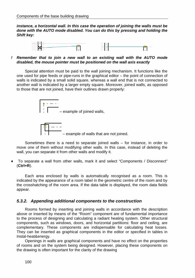
Components of the base building drawing
100
instance, a horizontal wall. In this case the operation of joining the walls must be done with the AUTO mode disabled. You can do this by pressing and holding the Shift key:
! Remember that to join a new wall to an existing wall with the AUTO mode disabled, the mouse pointer must be positioned on the wall axis exactly
Special attention must be paid to the wall joining mechanism. It functions like the
one used for pipe feeds or pipe-runs in the graphical editor – the point of connection of walls is indicated by a small solid square, whereas a wall end that is not connected to another wall is indicated by a larger empty square. Moreover, joined walls, as opposed to those that are not joined, have their outlines drawn properly:
– example of joined walls,
– example of walls that are not joined. Sometimes there is a need to separate joined walls – for instance, in order to
move one of them without modifying other walls. In this case, instead of deleting the wall, you can separate it from other walls and modify it.
♦ To separate a wall from other walls, mark it and select “Components / Disconnect”
(Ctrl+R). Each area enclosed by walls is automatically recognised as a room. This is
indicated by the appearance of a room label in the geometric centre of the room and by the crosshatching of the room area. If the data table is displayed, the room data fields appear.
5.3.2. Appending additional components to the construction
Rooms formed by inserting and joining walls in accordance with the description above or inserted by means of the “Room” component are of fundamental importance to the process of designing and calculating a radiant heating system. Other structural components, such as windows, doors, and horizontal partitions: floor and ceiling, are complementary. These components are indispensable for calculating heat losses. They can be inserted as graphical components in the editor or specified in tables in Instal-heat&energy.
Openings in walls are graphical components and have no effect on the properties of rooms and on the system being designed. However, placing these components on the drawing is often important for the clarity of the drawing

Components of the base building drawing
101
The properties of complementary components are similar to those of the fittings in
the graphical editor – they cannot stand alone. They can only be placed on the wall (window, door, opening) or within room area (horizontal partitions: floor, ceiling) to which they are assigned in terms of the drawing, and sometimes also in terms of data fields in the data table.
♦ To place a window, door or an opening in an existing wall:
1. Click the appropriate button on the „Components” toolbar – for an opening
in wall, for a window or for a door. The component inserting mode is enabled.
2. Position the mouse pointer on the wall axis at the point where the centre of the component (e.g. window) is to be located:
3. Press the left mouse button. The component is inserted at the indicated point of the wall:
4. If the mouse pointer is not exactly on the axis of the wall, the component is not inserted and an audible warning signal is sounded and an appropriate message is displayed in the status bar.
5. After inserting a wall with a component, a window for instance, these components are marked. Thus you can specify the window data at once. The width of the window is taken from the building structure data or a default value is adopted. To change the width and depth of the window enter the desired values into appropriate fields in the data table (window data are displayed below the wall data).
6. If the window is not oriented properly, drag the small square with an arrow , displayed near the window.
7. In the case of door, by dragging the small square with an arrow you can change both the side to which the door opens (outwards or inwards) and the direction of door opening (right or left):
8. To move a window, door or an opening, position the mouse pointer on the axis of the wall occupied by that component, press and hold the left mouse button and drag the component along the wall. You cannot move a window from one wall to another this way!

Components of the base building drawing
102
♦ To place a horizontal partition of the floor or ceiling type in an existing wall:
1. Click the appropriate button on the „Components” toolbar – for floor or
for ceiling. The component inserting mode is enabled. 2. Position the mouse pointer within the room area:
3. Press the left mouse button. The selected component is inserted in the room area within room axes and adapts it to the shape of the room below or above.
4. The inserted partition is marked. Thus you can specify the window data at once. 5. To insert several partitions of the floor or ceiling type into one room, repeat the
operations described above.
! If under the edited room there is (on the plan view of the storey below) more than one room, the horizontal partition – floor will only cover the part common to both rooms. Therefore, several such partitions have to be inserted. The same applies to rooms above.
5.3.3. Data of importance to floor heating design
Each of the structural components, that is a wall, a window assigned to a wall, a door or an opening in a wall, horizontal partition and also a room identified by the program, has defined parameters (properties), which can be reviewed and modified in the data table. The data table displays fields that characterise the component that is currently marked. These data may be specified when placing the components or later, when the drawing is complete. When inserting components, it is advisable to check and, if necessary, modify some of the data that have an impact on the appearance of the construction, such as lengths and widths of walls, widths of windows and doors, etc. Most of the data, however, particularly room data, are specified most conveniently after completing the drawing of walls and other graphical components.
Before starting to specify data you should also check program settings. The data
table should be displayed, it is also advisable to enable the LOCK mode to protect components against unintended displacement. To make data appending faster, use the available functions of simultaneous data entry.

Components of the base building drawing
103
Below is a list of construction component data that are particularly important in the
aspect of editing and calculating a radiant heating system. Short description and significance of each of the data is given.
Wall
- “Wall type” – depending on the type of wall the border of the effective heating zone is set off at a certain distance from the wall face. For internal and external walls this distance is defined in the general data of the.
- “HZ distance from wall” – for unusual cases specify the required distance between HZ and the wall.
Room
- “Room symbol” – serves the purpose of entering room name, which makes the drawing and results more clear.
- “ti/θi” – temperature inside the room. As the output of the radiant heating system depends on the difference between floor temperature and room temperature, this value is of great importance for the calculations.
- “ti/θi below” – temperature below the given room. This temperature is accounted for when floor structure is determined either automatically or manually. When you enter a value here, then respective fields in HZ data of the room will not be modifiable – the value specified here is transferred to HZ data. If you enter “-“ in the “Ti below” field, then no temperature will be defined and you will be able to specify different temperature for each HZ in the room.
- “Qreq/Φreq.”, “RH contribution [%]“, “Qrh/Φrh”, “Rad. contr. [%]” and “Qrad/Φrad” – determine the required output of terminal units in the room to be delivered by radiant and radiator heating. This value has a significant impact on the operating conditions of the circuits, floor structure and radiator sizing.
- “Area w.f.” – room surface area within wall faces. Value in brackets indicates area taken from drawing. If it is inconsistent with the real value, the wall lengths have to be modified on the drawing or the value in the table must be overwritten (although a precise drawing is preferred to overwriting the numerical value).
- “Room type” – defines how the room is used and the associated maximum temperatures of the floor surface. These values impose limitations on calculations. To specify maximum temperatures other than default, select “Other” and enter the desired values of floor surface maximum temperatures in the fields below (after selecting “Yes” in “Show RH data”).
! The loss across heated partition should be deduced from and losses from other
rooms where heat distribution has been specified should be added to the heat loss in room.
5.3.4. Complex cases encountered when editing construction
Solutions to some more complex cases of editing building construction are presented in this section.
Varying thickness of a wall within one straight segment:

Components of the base building drawing
104
♦ To introduce wall thickness variation: 1. Enter each segment of different thickness as a separate wall type component
and specify its thickness:
2. Move one of the walls so that the faces on one side of the walls form a straight line and ends of the walls coincide (after acquiring some skill it is possible to draw walls in this way right away; to do this you have to disable the AUTO mode, so that wall ends are not connected automatically):
3. Insert an additional wall segment to join the ends of walls of different thickness:
In a similar way you can join 3 walls, of which the two collinear walls are of
different thickness. The result should, for instance, look like the one below:
It is easier to solve this case by defining the thicker collinear wall as an asymmetrical wall:
5.4. Arrangement of floors in a schematic view
The only structural component on “Schematic view” sheets is the floor elevation label. This component, apart from its graphical functions, is also of importance in automatic duplication of storeys, inserting radiators above a floor, duplication of expanding groups and in automatic filling of terminal units symbols. This component is

Components of the base building drawing
105
not automatically associated with the arrangement of storeys specified in the “Building structure”.
By default after launching the program, only the “Plan view” type sheet is
displayed. To create a new worksheet select “Worksheets ...” in the “File” main menu, select “New”, select sheet type, change its name, if necessary, then click “OK” and “Close”.
! To be able to insert or modify floor elevations, activate the “Construction” tab.
To insert a floor elevation label into the project, select in the upper toolbar, move the mouse pointer into the drawing area and click in the selected spot. The floor arrangement is inserted. This component, when marked, has a frame with handles in the form of small squares. By dragging the frame handle you change the dimensions of the component. This way you can contract or expand the range of floors displayed.
There may be several storeys within one “Floor elevation label” type component. You can modify storey elevations both in data table and using the mouse.
! Storey elevations can be modified with the mouse only when the floor elevation
component is marked. After clicking the floor elevation component in the data table, its data are
displayed:
- Basement elevation – specification of basement ceiling elevation. - Ground floor elevation – elevation of first storey. - Elevation difference – difference of elevations of a typical storey. - Floor thickness – thickness of floor above for all storeys. - Ready floor – thickness of floor for all storeys. - False ceiling – thickness of false ceiling for all storeys. Forms complete structure
of floor in conjunction with the thickness of floor and floor above. - Lowest storey number – number of first storey described by selected
component. Important when terminal unit symbols are filled in automatically. - Storeys ... – after opening the window associated with this field, you can modify
separately the elevation of each storey, thickness of floor, floor above and false ceiling and position of label of each storey.
- Show elevations – specifies whether the label is to be displayed for the floor proper or for the complete floor.
- dH in isometric drawing – difference of elevations between co-ordinate system of the selected component and the absolute co-ordinate system.
- Font – style, size and colour of font used in storey elevation labels. - Line type – style, colour and thickness of the line used to draw the floors.
! After modifying the “Basement elevation”, “Ground floor elevation”, “Elevation
difference” or “Floor thickness” fields, the elevations of all storeys are changed, even if they were specified separately in the “Storeys ...” field.

Components of the base building drawing
106
“dH in isometric drawing” is useful when drawing a diagram of distribution
network as an isometric drawing and risers are drawn in traditional way. Radiators must have an absolute coordinate system assigned, where identical elevations are determined.

Components that make up the system diagram
107
6. COMPONENTS THAT MAKE UP THE SYSTEM DIAGRAM
6.1. Basic components of a radiator heating system
Below is a description of the principal components used in the program to construct a radiator heating system. All these components are in the upper toolbar of the “Central” tab. Some of them have a hydraulic representation, while others are just drawings, which are not listed in data tables. As in the case of data (properties) of these components – some are represented in the drawing only, while other are reflected in data tables.
The components mentioned below are designed for insertion into the „Installation”
layer of the project. The “Print” tab is designed for print preview and print settings only.
6.1.1. Radiator
Radiator is a terminal unit the size of which the application tries to determine or to verify the imposed size. You should indicate an excessive pressure-reducing device on the radiator or one of its circuit pipes. The appearance of a radiator placed on a plan view differs from that of a radiator on a schematic view.
Button on the “Central” toolbar: Appearance on screen (plan view):
integrated radiator:
radiator with side connection: Appearance on screen (schematic view):
integrated radiator:
radiator with side connection:
tube-type radiator: ,
segmented radiator:

Components that make up the system diagram
108
bathroom radiator:
modular radiator: “Radiator” component data:
TU symbol Text field. You can enter a caption that will identify the radiator unambiguously. In room Text field. You cannot enter the name of the room where the radiator is installed – you must select the room from a list. When connections are checked, the radiators are automatically assigned to rooms within the area of which they are placed in plan view. Contribution [%] Numerical field. Radiator output as percentage of heat demand in room. The default setting (auto) assigns contribution on the basis of heat loss calculation results, which take into account other heat sources in the room. Q/Φ [W] Numerical field. Required output of terminal unit. Value in brackets indicates that output determined from contribution. Type Selection field. Radiator type – select from selected manufacturer’s catalogue or from among radiators not in catalogue. Size Selection field. Specified radiator size. You can select from list or retain the default size (size). Size limits Compound field. Manner of sizing radiator with existing restrictions being accounted for. After clicking on an arrow to the right of the field, a new window is opened where you can specify the height, length and depth of radiator (H, L and D fields displayed in window are described below). You can specify the way the radiator is to be sized when restrictions are imposed: specify size, select the smallest radiator from a range or fit the radiator to a recess. The “User specified” option enables selection of radiator in accordance with specified dimension – the first radiator found that matches the specified dimension is selected. You can specify one, two or all three dimensions of radiator. The “Smallest in range” option enables selection of the smallest dimension within specified range determined by minimum and maximum dimensions. This

Components that make up the system diagram
109
means that the first radiator found that matches “Lmin” (minimum dimension within range) is selected. The “To recess” option enables selection of radiator that matches the dimensions of recess (recess dimension and occupied dimension is specified). This option enables selection of radiator that has maximum possible dimensions to match the recess. This means that the first radiator found that matches “Lmax” (maximum dimension within range) is selected. H user specified, H min/max, H recess Compound field. Height of radiator. Depending on the radiator sizing method, the title changes appropriately. L user specified, L min/max, L recess Compound field. Length of radiator. Depending on the radiator sizing method, the title changes appropriately. D user specified, D min/max Compound field. Depth Length of radiator. Depending on the radiator sizing method, the title changes appropriately. Connection type Compound field. Select terminal unit connection type and specify, if necessary, allowances for sizing: enclosure type and location of radiator – a window opens after clocking a button to the right of the field. Terminal unit conn. system Selection field. System of terminal unit connection. Select from a list, depending on selected pipe system and connection systems defined therein. ti/θi [0C] Temperature in room where the radiator is installed. Availability Selection field. When sizing a radiator, it can be looked for among all radiators available in catalogue (complete range of delivery) or among preferred radiators only (in stock). You can also leave the choice to be made in calculation options. To left of riser Selection field. Specifies whether the radiator is installed to the left of the riser. H [m] Numerical field. Elevation of radiator. It can be determined automatically (value in brackets) or specified by the user. To revert to automatic determination enter “?”. ∆t/∆θ [0C] Numerical field. Specified temperature drop across the radiator. Value in brackets indicates the default value. Rad. share in 1-pipe system Numerical field. Share of flow in radiator in the total flow in a single pipe systems. The value is assigned by default to all new radiators, and then can be

Components that make up the system diagram
110
modified individually. Value in brackets indicates default value determined from the value specified in general data. Pipe feed diam. Selection field. Specify type or diameter of pipe feed for radiators not in catalogue. Component status Selection field. Select from list the current status of component: existing or under design. Label type Selection field. Select from list the type of radiator label in drawing. After selecting “Configure”, a component appearance window is opened, where you can create (by copying) and configure the appearance of components in the drawing. After specifying a new label, it is then available in a pull down list in the table. Advance dwg. Selection field. Select from list the radiator circuit pipe on plan view to be drawn beside the radiator. The default setting is the return pipe-run.
advance: supply advance: return
Fixing point Selection field. Specify where in the drawing the fixing point is to be located. The fixing point is the point from which the radiator will be enlarged / reduced when its size is changed.
♦ There is a function that enables fast arrangement of radiators under all external
windows. To use this function select “Insert radiators under external windows” from the
“Components” menu. You can also use , buttons in the “Central” toolbar.
6.1.2. Terminal unit with imposed pressure drop
Terminal units with imposed pressure drop are used to describe, for instance, heaters or fan coil units. These components are not selected from catalogues..
Button on the “Central” toolbar: Appearance on screen (plan / schematic view):
Components that make up the system diagram
111
“Terminal unit” component data:
TU symbol Text field. You can enter a caption that will identify the radiator unambiguously. In room Text field. Room where the terminal unit is installed must be selected from list. If heat loss calculations where done in Instal-heat&energy, the room name is automatically entered into the table. Q/Φ [W] Numerical field. Required output of terminal unit. Comp. flow resist. Selection field. Type of flow resistance specified for the terminal unit – select from list: pressure drop known / zeta known / Kv known. Zeta / Kv / Pressure drop Numerical field. Flow resistance in terminal unit. You can enter the values directly using appropriate brackets: square brackets [] for zeta, round brackets () for Kv, braces {} for pressure drop. After entering a value in appropriate brackets, the component flow resistance is automatically modified. Water capacity [dm3] Numerical field. Water capacity. ti/θi [0C] Numerical field. Temperature in room where the terminal unit is installed. ∆t/∆θ [0C] Numerical field. Specified temperature drop across the terminal unit. Value in brackets indicates the default value. H [m] Numerical field. Elevation of terminal unit. It can be determined automatically (value in brackets) or specified by the user. To revert to automatic determination enter “?”. Height [m] Numerical field. Height of terminal unit. Length [m] Numerical field. Length of terminal unit. Drawing type Selection field. Manner of drawing the component selected from list. Drawing Separate drawing of terminal unit. If “Drawing type” is indicated as “Drawing”, then here you can select one of the loaded drawings or add a new one.

Components that make up the system diagram
112
Connection type Selection field. Select connection type from list. Pipe feed diam. Selection field. Specify type or diameter of pipe feed for terminal unit. Component status Selection field. Select from list the current status of component: existing or under design. Affects only bill of material. Label type Selection field. Select from list the type of terminal unit label in drawing. After selecting “Configure”, a component appearance window is opened, where you can create (by copying) and configure the appearance of components in the drawing. After specifying a new label, it is then available in a pull down list in the table.
6.1.3. Heating riser
Heating risers are treated as terminal units. They can only be inserted into a “Schematic view” type sheet.
Button on the “Central” toolbar: Appearance on screen (schematic view):
“Heating riser” component data:
TU symbol Text field. You can enter a caption that will identify the radiator unambiguously. Drawing type Selection field. Drawing type: single / double. Q/Φ [W] Numerical field. Required output of terminal unit. ∆t/∆θ [0C] Numerical field. Specified temperature drop across the terminal unit. Value in brackets indicates the default value.

Components that make up the system diagram
113
Pipe type Selection field. Type of pipe used in the heating riser. You can select it from a list opened by clicking the button to the right of the field or enter directly using a letter shortcut. Length [m] Numerical field. Length of terminal unit. ti/θi [0C] Numerical field. Temperature in room where the terminal unit is installed. H [m] Numerical field. Elevation of the centre of terminal unit. It can be determined automatically (value in brackets) or specified by the user. To revert to automatic determination enter “?”. Component status Selection field. Select from list the current status of component: existing or under design. Affects only bill of material. Label type Selection field. Select from list the type of terminal unit label in drawing. After selecting “Configure”, a component appearance window is opened, where you can create (by copying) and configure the appearance of components in the drawing. After specifying a new label, it is then available in a pull down list in the table.
6.1.4. Pipe-run
Pipe-run in the graphical editor is exactly the same as a pipe-run in the entire package. It is a section of the system of constant calculation flow rate. You can place fittings and “miscellaneous fittings” (not shown on drawing) on it. A pair of pipe-runs exists only as long as the pipe-run is being drawn; after it is completed the pair breaks down into two pipe-runs.
A pipe-run may consist of many segments. Points within a pipe-run are depicted in the form of diamonds, whereas terminal points are shown as squares.
Button on the “Central” toolbar: , or, a pair of pipe-runs: Appearance on screen (colours: supply = red, return = blue):
“Pipe-run” component data:
Pipe-run number Numerical field. Unique symbol assigned automatically to a pipe-run. May be changed by the user. Numbers of supply and return pipe-runs are identical. The

Components that make up the system diagram
114
system is numbered in the order from the source to terminal units. When a pipe-run is connected to a preceding pipe-run without branching, then it have the same number followed by subsequent letters: _a, _b, _c, etc.
Every check of connections or launching of calculations cause automatic renumbering of the pipe-runs. User-specified pipe-run numbers remain unchanged, and become the starting point of a new numbering sequence (if, for instance, you assign number 40 to a pipe-run that follows pipe-run no. 23, then the following pipe-runs will be assigned numbers 41, 42, 43, etc.). You can take advantage of this option when numbering risers or pipe-runs of apartment systems. When you assign defined numbers to riser segments or systems (e.g. 1000, 2000), then all pipe-runs within the given riser or system will have subsequent numbers assigned: 1001, 1002 or 2001, 2002, etc.
Length [m] Numerical field. May be determined by the application – in this case it is shown enclosed in brackets. If the user enters the length, the application abandons length determination for that pipe-run. You can revert to automatic length determination by entering “?”. Pipe type Selection field. You can select it from the list opened by clicking the button on the right side of the field or enter it directly using a letter shortcut. Location Selection field. Location of the pipe-run in the system being designed. Name in brackets indicates the default name. You can change it by selecting a name from list. To revert to automatic determination enter “?”. The location of a component in the system is important in relation to calculation options, where various diameter sizing options may be defined for various locations. The entire system is divided into radiator circuit pipes, apartment system, risers and network (distribution to risers). Connection cat. and type Selection field. Catalogue and, if necessary, type of pipe fittings used to make junctions (tees) and connections. The default setting is “ As pipe-run catalogue”. The field does not apply to elbows, the type of which is specified in the field below.
specifed numbers

Components that make up the system diagram
115
Bend type Selection field. Type of component accounted for in calculations for every elbow shown in drawing. You can select it from a catalogue or enter it using a letter shortcut. Default setting: “(size)”. Miscellaneous fittings Compound field. Other fittings not shown on diagram. Select from catalogue and you can use a macro. Ambient temperature [oC] Numerical field. Temperature of the pipe-run environment. Default value (in brackets) is taken from general data. Insulation [mm] Selection field. You can select insulation type from catalogues loaded into the project. Thickness may be specified or determined automatically. The (default) value indicates that insulation type for the pipe-run is taken from general data. Component status Selection field. Select from list the current status of component: existing or under design. Elevation [m] Numerical field. Determined by the application (value in brackets) or specified by the user. You can revert to automatic determination by entering “?”. Gains in room Selection field. You can specify the room in which heat gains from the given pipe-run are to be accounted for. By default the room is selected automatically. Line style Selection field. Select from list the appearance of the pipe-run or configure it – component appearance window is opened. After placing a valve or other fitting component on a pipe-run, its list of properties (data) is supplemented with properties of the component inserted.
6.1.5. Single-pipe connection
A single-pipe connection is treated as a pipe-run. In the graphical editor, however, it is marked out to enable creating a single-pipe portion in a network – in this case slightly different rules are applied to radiator connections: you can connect the return side of one radiator with the supply side of another radiator.
Button on the “Central” toolbar: Appearance on screen (green):

Components that make up the system diagram
116
“Single-pipe connection” component data – same data set as for a pipe-run.
6.1.6. By-pass pipe-run, pipe-run with no flow
By-pass pipe-runs are used to insert additional fragments of the system, where fitting components (e.g. pressure relief valves) may be installed.
Pipe-runs with no medium flow are used to connect components of expansion vessel type or to create a vent system.
Button on the “Central” toolbar: and Appearance on screen (pink and grey):
and “By-pass pipe-run” and “Pipe-run with no flow” component data – same data
set as for a pipe-run.
6.1.7. Manifold
The program differentiates, in drawing terms, between apartment manifolds and manifolds used for networking the system, e.g. at basement level. To facilitate editing, a symbol for a pair of manifolds has been introduced. The symbol is a (inseparable) duplicate of the manifold for supply and return.
Manifolds in radiator heating do not have to be associated with equipment catalogues.
Buttons on the “Central” toolbar: Appearance on screen (plan / schematic view):
“Manifold” component data:
Symbol Text field. The symbol is defined automatically, when the manifold in the drawing is within a room, or it can be specified by the user. The symbol is used to identify the manifold when editing data and in the tables of results.
Components that make up the system diagram
117
No. of outlets / No. of outlet pairs Numerical field. The number of outlets must be consistent with the number of pipe-runs or pipe feeds connected. When drawing a system starting from the manifold, the number of outlets is automatically incremented (the manifold is enlarged) as required. The number may be specified – then all outlets must be connected or some of them must be defined as spare. of that spare Numerical field. Number of spare ports, which may be used later. These are not accounted for in calculations. When, for instance, only radiant heating calculations are done, they may be treated as designed for connecting additional radiators not included in the given project. This enables specifying in the bill of materials a manifold with the number of outlets greater than the number of connected heating circuits. Manifold type Selection field. Manifold type selected from catalogue. If “(default)” is specified, then the type specified in general data is adopted. If a manifold with control elements is selected, valve data are displayed in the table below the manifold data. Supply/return arrangement Selection field. The position of the supply part of the manifold in relation to the return part (for angle of 0°). This only has an effect on the drawing and enables the adaptation of the manifold drawing to the actual arrangement of the supply and return parts of the manifold. Opposite arrangement of the parts of the manifold may result in the crossing over of pipes in the drawing. Cabinet type Selection field. Select cabinet type from catalogue. If “(default)” is specified, then the type specified in general data is adopted. Cabinet axis above floor [m] Numerical field. Distance between cabinet axis and the floor. The required number of pipes to construct vertical route will be accounted for in the bill of materials. Show RH data Selection field. This field enables hiding or displaying additional data associated with radiant heating. The default setting is “No”. When you enter “Yes”, additional fields described above appear in the table. ∆t/∆θ min OZ Numerical field. Minimum temperature drop for HZ in occupied zone. ∆t/∆θ max OZ Numerical field. Maximum temperature drop for HZ in occupied zone. ∆t/∆θ min PZ Numerical field. Minimum temperature drop for HZ in peripheral zone.
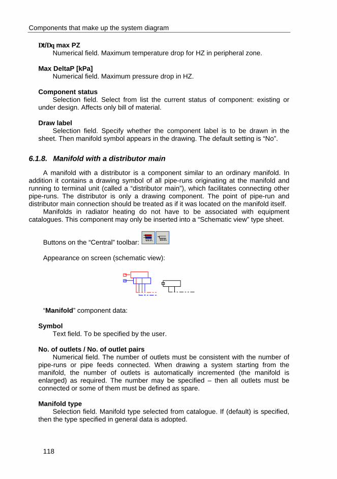
Components that make up the system diagram
118
∆t/∆θ max PZ Numerical field. Maximum temperature drop for HZ in peripheral zone. Max DeltaP [kPa] Numerical field. Maximum pressure drop in HZ. Component status Selection field. Select from list the current status of component: existing or under design. Affects only bill of material. Draw label Selection field. Specify whether the component label is to be drawn in the sheet. Then manifold symbol appears in the drawing. The default setting is “No”.
6.1.8. Manifold with a distributor main
A manifold with a distributor is a component similar to an ordinary manifold. In addition it contains a drawing symbol of all pipe-runs originating at the manifold and running to terminal unit (called a “distributor main”), which facilitates connecting other pipe-runs. The distributor is only a drawing component. The point of pipe-run and distributor main connection should be treated as if it was located on the manifold itself.
Manifolds in radiator heating do not have to be associated with equipment catalogues. This component may only be inserted into a “Schematic view” type sheet.
Buttons on the “Central” toolbar: Appearance on screen (schematic view):
“Manifold” component data:
Symbol Text field. To be specified by the user. No. of outlets / No. of outlet pairs Numerical field. The number of outlets must be consistent with the number of pipe-runs or pipe feeds connected. When drawing a system starting from the manifold, the number of outlets is automatically incremented (the manifold is enlarged) as required. The number may be specified – then all outlets must be connected or some of them must be defined as spare. Manifold type Selection field. Manifold type selected from catalogue. If (default) is specified, then the type specified in general data is adopted.

Components that make up the system diagram
119
Supply/return arrangement Selection field. The position of the supply part of the manifold in relation to the return part (for angle of 0°). Component status Selection field. Select from list the current status of component: existing or under design. Affects only bill of material. Draw label Selection field. Specify whether the component label is to be drawn in the sheet. Then manifold symbol appears in the drawing. The default setting is “No”.
6.1.9. Boiler and Source
Boiler and source are components that form the main supply point of the system. There may be several heat sources or boilers on one sheet. If there are several sources in one project, systems supplied from different sources cannot be connected to each other in any way.
A project does not have to include a heat source in the drawing – in such case select “Create virtual connections” in general data to enable correct calculations. In this case a virtual source is created, the supply temperature of which is taken from general data of the project.
Buttons on the “Central” toolbar: Appearance on screen (plan view):
Appearance on screen (schematic view):
“Boiler” / “Source” component data:
Symbol Text field. Displayed in project – no effect on calculations.

Components that make up the system diagram
120
Supply temp. Numerical field. Supply temperature of the given source. Value in brackets indicates default value taken from general data. Source flow resist. Selection field. Type of flow resistance specified for the source – select from list: pressure drop known / zeta known / Kv known. Zeta / Kv / Pressure drop Numerical field. Value for calculating flow resistance in source. You can enter the values directly using appropriate brackets: square brackets [] for zeta, round brackets () for Kv, braces {} for pressure drop. After entering a value in appropriate brackets, the “Source flow resistance type” field is automatically modified. Use Selection field. Indicate the use of the source – heating or cooling. Upon selection the fields in the data table are modified accordingly. Medium type Selection field. The default medium in the system is water. You can specify other medium – in this case an additional field appears in the table: “Medium contribution”. Medium contribution [%] Numerical field. Contents (percentage) of the medium. Specified for medium other than water (e.g. glycol). Available pressure [kPa] Numerical field. The default setting is “(size)”. You can specify a value, which then will be accounted for in calculations. Static head [MPa] Numerical field. The default static head is 0.6 MPa. You can change this value. Water capacity of source [dm3] Numerical field. Water capacity of the source. ts/θs min. RH Numerical field. Lower limit of temperature range for radiant heating supplied from the source. Value taken into account when optimising supply temperature. ts/θs max. RH Numerical field. Upper limit of temperature range for radiant heating supplied from the source. Value taken into account when optimising supply temperature. Heat source appearance Selection field. Select from list the manner of drawing the source. Connections Selection field. Select from list the manner of drawing the supply and return lines in relation to each other.

Components that make up the system diagram
121
Conn. spacing in dwg. Numerical field. Spacing between connection points in drawing. H [m] Numerical field. Elevation of source. Determined by the application (value in brackets) or specified by the user. You can revert to automatic determination by entering “?”. Pipe feed diam. Selection field. Select from list the type and diameter of pipe feed for the heat source. Connection type Selection field. Select from list the arrangement of pipe connection symbols for boiler. Drawing type Selection field. Select from list the manner of drawing the boiler. Drawing Separate drawing for boiler or source. If “Drawing type” or “Heat source appearance” is indicated as “Drawing”, then here you can select one of the drawings loaded into the “Drawings gallery” or add a new one. Label type Selection field. Select from list the type of boiler label in drawing. After selecting “Configure”, the “Component appearance” window is opened. This window contains tabs with components available in the project, the labels of which can be configured. You can create (by copying) and configure the labels of components in the drawing. After specifying a new label, it is then available in a pull down list in the table. Component status Selection field. Select from list the current status of component: existing or under design. Affects only bill of material.
6.1.10. Remote connection
This component is used for providing a remote connection of a pair of pipe-runs (supply and return) or of pipe-runs (supply only or return only). The remote connection is indicated with a symbol and assigned destination sheet with which it is associated. Within a project these components should be placed in pairs of the same symbol. A remote connection can be used within one sheet or to make system connections between sheets.
Button on the “Central” toolbar: Appearance on screen (plan / schematic view):

Components that make up the system diagram
122
“Remote connection” component data:
Dest. worksheet Selection field. Select from list with which sheet of the project the connection is to be associated. Symbol Text field. Symbol of remote connection that identifies the component unambiguously. Label type Selection field. Select from list the type of connection label in drawing. Connections Selection field. Select from list the manner of drawing the supply and return lines in relation to each other or indication that the remote connection applies to supply only or to return only. Arrows Selection field. Toggle on/off the drawing of arrows.. Conn. spacing in dwg. Numerical field. Spacing between connection points in drawing. Font Compound field. Select style, size and colour of font. Height Numerical field. Height of font in label.
6.1.11. Automatic schematic view
This is a remote connection component designed to make schematic views of system parts on the basis of a drawn and calculated plan view diagram. Automatic schematic view is identified by a symbol and assigned destination sheet with which it is associated.
To put into effect an automatic schematic view a “Remote connection” component must be present in the plan view sheet and an “Automatic schematic view” component in the schematic view sheet.
This component may only be inserted into a “Schematic view” type sheet.
Button on the “Central” toolbar: Appearance on screen:

Components that make up the system diagram
123
“Automatic schematic view” component data:
Dest. worksheet Selection field. Select from list with which sheet of the project the connection is to be associated. Symbol Text field. Symbol of remote connection that identifies the component unambiguously. Label type Selection field. Select from list the type of connection label in drawing. Supply point above reference level Numerical field. Distance between the point indicating connection of supply and the reference level. The reference level is drawn with a broken line. Return point above reference level Numerical field. Distance between the point indicating connection of return and the reference level. TU distance from reference level Numerical field. Distance between the terminal unit and the reference level in the drawing. Font Compound field. Select style, size and colour of font. Height Numerical field. Height of font in label.
6.1.12. Riser as a drawing
This is just a drawing component – it is not subject to calculations. When using remote connections in the project that link individual sheets, this component is used to indicate points in the plan view where the riser is located – in other words, the point where vertical pipes cross the floor or ceiling.
Button on the “Central” toolbar: Appearance on screen:

Components that make up the system diagram
124
“Riser as drawing” component data:
Symbol Text field. Symbol that identifies the component unambiguously. Update on other storeys Selection field. If another “Riser as drawing” was inserted on other storey and the same symbol was assigned to it, the riser will be placed in the location of identical coordinates and its relative position will be controlled. Interaction radius Numerical field. Interaction radius is the range within which it “captures” remote connections and draws pipe-runs. This is represented by a circle radius. Conn. spacing in dwg. Numerical field. Spacing between connection points in drawing.
6.1.13. Three-way valve
3-way valves are components, which stand alone in the project – they are not inserted onto pipe-runs, as are other fitting components. There is now flow in the bypass pipe-run in the calculation condition of the system, i.e. the 3-way valve is sized for “full flow”.
Button on the “Central” toolbar: Appearance on screen (plan / schematic view):
“3-way valve” component data:
Symbol Text field. Symbol that identifies the component unambiguously. 3-way valve ... Selection field. Select valve type from loaded catalogue or assign the value of known Kv, zeta or pressure drop. Zeta / Kv / Pressure drop (optional) Numerical field. You can enter the values directly square brackets [] for zeta, round brackets () for Kv, braces {} for pressure drop. Applies only to components not in catalogue.

Components that make up the system diagram
125
Label location Selection field. Designed to move the label text. Clicking the button to the right of the field opens a special window with four arrows. Clicking the arrows makes the label move in steps in the selected direction. This field is useful when moving multiple valve labels after marking a group of valves. You may also move the valve label by dragging the symbol. Label type Selection field. You can define various manners of describing the valve. Here you can indicate which label will be used for the given valve or you can open an appearance configuration window. After defining a new label it is then available in the pull-down list in the table. Rotate dwg. Selection field. Manner of drawing the valve (parallel orientation, vertical orientation, etc.). Align horizontally Selection field. Align label horizontally. Head (optional) Selection field. Select valve head from catalogue list. Inlet diam. (optional) Selection field. In case of a valve with known flow resistance you can select from list its inlet diameter. Outlet diam. (optional) Selection field. In case of a valve with known flow resistance you can select from list its outlet diameter. DP min. [kPa] Numerical field. Minimum pressure drop across valve. Value in brackets is default value specified in calculation options. You may also specify the value individually. Component status Selection field. Select from list the current status of component: existing or under design. Affects only bill of material.
6.1.14. Four-way valve
4-way valves are components which stand alone in the project – they are not inserted onto pipe-runs, as are other fitting components. Connection of a valve is effected by inserting supply and return pipe-runs that link the valve with the system and which are accounted for in flow calculations. On a by-pass pipe-run there is no flow under the calculation conditions of the system, i.e. a 4-way valve is calculated for the “full flow” condition.

Components that make up the system diagram
126
Button on the “Central” toolbar: Appearance on screen (plan / schematic view):
“4-way valve” component data:
Symbol Text field. Symbol that identifies the component unambiguously. 4-way valve ... Selection field. Select valve type from loaded catalogue or assign the value of known Kv, zeta or pressure drop. Zeta / Kv / Pressure drop (optional) Numerical field. You can enter the values directly square brackets [] for zeta, round brackets () for Kv, braces {} for pressure drop. Applies only to components not in catalogue. Label location Selection field. Designed to move the label text. Clicking the button to the right of the field opens a special window with four arrows. Clicking the arrows makes the label move in steps in the selected direction. This field is useful when moving multiple valve labels after marking a group of valves. You may also move the valve label by dragging the symbol. Label type Selection field. You can define various manners of describing the valve. Here you can indicate which label will be used for the given valve or you can open an appearance configuration window. After defining a new label it is then available in the pull-down list in the table. Rotate dwg. Selection field. Manner of drawing the valve (parallel orientation, vertical orientation, etc.). Align horizontally Selection field. Align label horizontally.

Components that make up the system diagram
127
Head (optional) Selection field. Select valve head from catalogue list. Inlet diam. (optional) Selection field. In case of a valve with known flow resistance you can select from list its inlet diameter. Outlet diam. (optional) Selection field. In case of a valve with known flow resistance you can select from list its outlet diameter. DP min. [kPa] Numerical field. Minimum pressure drop across valve. Value in brackets is default value specified in calculation options. You may also specify the value individually. Component status Selection field. Select from list the current status of component: existing or under design. Affects only bill of material.
6.1.15. Mixer (temperature reducer)
This component represents a mixer (temperature reducer) used to connect floor heating systems.
Button on the “Central” toolbar: Appearance on screen (plan / schematic view):
“Mixer” component data:
Symbol Text field. Symbol that identifies the component unambiguously.
Source Terminal
units

Components that make up the system diagram
128
Mixer type Selection field. Type of mixer. By default an arrangement of 3-way valve and pump is assumed as a mixer. You can indicate other type in the pull-down list. Outlet temp. Numerical field. Temperature at the outlet of mixer. The value may be determined automatically when the mixer feeds a radiant heating system (using information on connected circuits and manifolds of radiant heating system). You can specify a value or enter “?” to revert to automatic outlet temperature determination. Component status Selection field. Select from list the current status of component: existing or under design. Affects only bill of material. ts/θs min. RH Numerical field. Lower limit of temperature range for radiant heating. Value taken into account when optimising supply temperature. ts/θs max. RH Numerical field. Upper limit of temperature range for radiant heating. Value taken into account when optimising supply temperature. After selecting mixer type, the table displays below the mixer data the data of existing valves and pump. Valve types must be specified.
6.1.16. Bypass bottle
This component represents a bypass bottle. It may only be inserted into a “Schematic view” type sheet.
Button on the “Central” toolbar: Appearance on screen (schematic view):
“Bypass bottle” component data:
Symbol Text field. Symbol that identifies the component unambiguously. Drawing type Selection field. Select from list the manner of drawing the component.

Components that make up the system diagram
129
Pipe feed diam. Selection field. Select from list the type and diameter of pipe feed for the bypass bottle. Component status Selection field. Select from list the current status of component: existing or under design. Affects only bill of material.
6.1.17. Expansion vessel
This component represents an expansion vessel. It is not accounted for in calculations and is just a drawing symbol. It can be connected to the system by means of a pipe-run with no flow.
This component may only be inserted into a “Schematic view” type sheet.
Button on the “Central” toolbar: Appearance on screen (schematic view):
“Expansion vessel” component data:
Inlet Selection field. Orientation of inlet. H [m] Numerical field. Elevation of the component. Determined by the application (value in brackets) or specified by the user. You can revert to automatic determination by entering “?”. Component status Selection field. Select from list the current status of component: existing or under design. Affects only bill of material.
6.1.18. Fitting components placed on pipe-runs
Fitting components cannot stand alone in the project, they can only be inserted into another basic component.
All valves inserted into the system must exist in catalogues or have their pressure drop or Zeta/Kv values specified. Orifice plates, air bleeders, filters, thermometers and other have no association with catalogues.
There are some limitations on the number of components placed in this manner, irrespective of their use or function.

Components that make up the system diagram
130
- Valves (placed on pipe-runs): /
- Orifice plate (placed on pipe-run): “Valve” component data:
Valve Selection field. Select valve from catalogue or specify Kv, zeta or pressure drop. After selecting valve type from list the drawing symbol is modified accordingly. Zeta / Kv / Pressure drop (optional) Numerical field. You can enter the values directly square brackets [] for zeta, round brackets () for Kv, braces {} for pressure drop. Applies only to components not in catalogue. Label location Selection field. Designed to move the label text. Clicking the button to the right of the field opens a special window with four arrows. Clicking the arrows makes the label move in steps in the selected direction. This field is useful when moving multiple valve labels after marking a group of valves. You may also move the valve label by dragging the symbol. Label type Selection field. You can define various manners of describing the valve. Here you can indicate which label will be used for the given valve or you can open an appearance configuration window. After defining a new label it is then available in the pull-down list in the table. Rotate dwg. Selection field. Manner of drawing the valve (parallel orientation, vertical orientation, etc.). Align horizontally Selection field. Align label horizontally. Head (optional) Selection field. Select valve head from catalogue list. Inlet diam. (optional) Selection field. In case of a valve with known flow resistance you can select from list its inlet diameter. Outlet diam. (optional) Selection field. In case of a valve with known flow resistance you can select from list its outlet diameter. DP min. [kPa] Numerical field. Minimum pressure drop across valve. Value in brackets is default value specified in calculation options. You may also specify the value individually.

Components that make up the system diagram
131
Draw imp. tube / bleed pipe. For throttling type differential pressure valves it is necessary to have a component that will provide a pressure impulse. When a pressure regulator is inserted, two valves are placed on pipe-runs. These valves must have appropriate types assigned in the table. These valves are connected in the drawing by means of an impulse tube. This impulse tube can be hidden or displayed in the drawing.
Other fittings placed on pipe-runs:
- Fixed points / , sliding points / ,
- Components of the type: 90° deflection , 45° deflection , 90°
elbow , running trap , offset , expansion component (you can select a defined component from manufacturer’s component or retain the default setting).
- Air bleeders / , thermometers / , pressure
gauges / , safety valves , partition crossing ,
- Restrictors: ,
- Filters / , heat meters / , strainers / (you can select defined components from “miscellaneous component” catalogues or just specify pressure drop in kPa or zeta / Kv value).
6.1.19. Fitting components placed on terminal units
The only fittings you can place on radiators are valves designed for this and air bleeders.
- Radiator couplings:
- Integrated radiator couplings:
- Air bleeders: /
6.1.20. Fitting components placed on manifolds
Fitting components that can be placed on manifolds include:
- Manifold sets:
- Pumping and mixing sets:
- Sets for installing meters:

Components that make up the system diagram
132
These components should be selected from catalogues.
6.1.21. Pumps
- Pumps: / – pumps have no catalogues in the application. The following fields are displayed in the data table for this component:
Pump ... Text field. You can enter a pump symbol. Del. head [kPa] Numerical field. The value of delivery head of the pump – specified by user or determined automatically. Value in brackets indicates value determined by the program (enter ‘?’ to have the program determine the value). Desc. table Selection field. You can modify the display of pump label in the drawing. Label type Selection field. You can define various manners of describing the pump. Here you can indicate which label will be used for the given pump or you can open an appearance configuration window. After defining a new label it is then available in the pull-down list in the table. Label location Selection field. Designed to move the label text. Clicking the button to the right of the field opens a special window. You may also move the pump label by dragging the symbol. Inlet diam. Selection field. Select from list the inlet diameter of pump. Outlet diam. Selection field. Select from list the outlet diameter of pump.
6.1.22. Special components
- Pressure differential gauge and pressure signal are used to measure the calculation pressure differential between any two points of the system. To measure pressure difference between selected points of the system, place a pressure gauge at one point of the pipe-run, and a pressure signal at the other point. Then click the symbol on the pressure gauge and drag it to the point where the pressure signal is placed. The two components will be linked together:

Components that make up the system diagram
133
6.2. Basic radiant heating units in the system
6.2.1. Heating floor
The concept of heating zone (HZ in short) as used in this application means a single circuit (in other words a loop) of radiant heating – part of heated floor or wall covered by one loop of pipe which starts and ends at a manifold. Therefore, if – for example – maximum length of pipe is exceeded and the circuit has to be divided into smaller circuits, the application divides HZ into, for instance, two smaller HZ’s.
! Heating zone is not equivalent to a single zone of jointless floating floor slab
with heating pipes immersed in it, separated from the walls and other slabs by joints. One slab may include several circuits, and consequently it may consist of several HZ’s. If, in construction terms, a given circuit is to form a separate floor slab, it should be singled out using joints. Division without joints enables defining several circuits within one floor slab.
The “Heating floor” component is inserted into “Plan view” type sheets only and is
placed within room area. By default the HZ is inserted over the entire area of the room. When you right click the HZ label a pop up menu appears where you can select
“Change type to freely modifiable”. “Handles” appear on the edges of the floor which enable changing the size and shape of floor in the room. This operation should only be performed in special cases.
A coloured triangle in the lower corner of each heating zone indicates the
thickness of floor built up (structure). By default the “Floor built up thickness designation” drawing option is checked. In the corner of every HZ a triangle appears, the colour of which depends on the floor built up determined automatically or specified by the user.
Additionally a legend may be placed in the drawing to explain the designations (see section 6.6.)
Button on the “Radiant” toolbar: Appearance on screen (plan view):
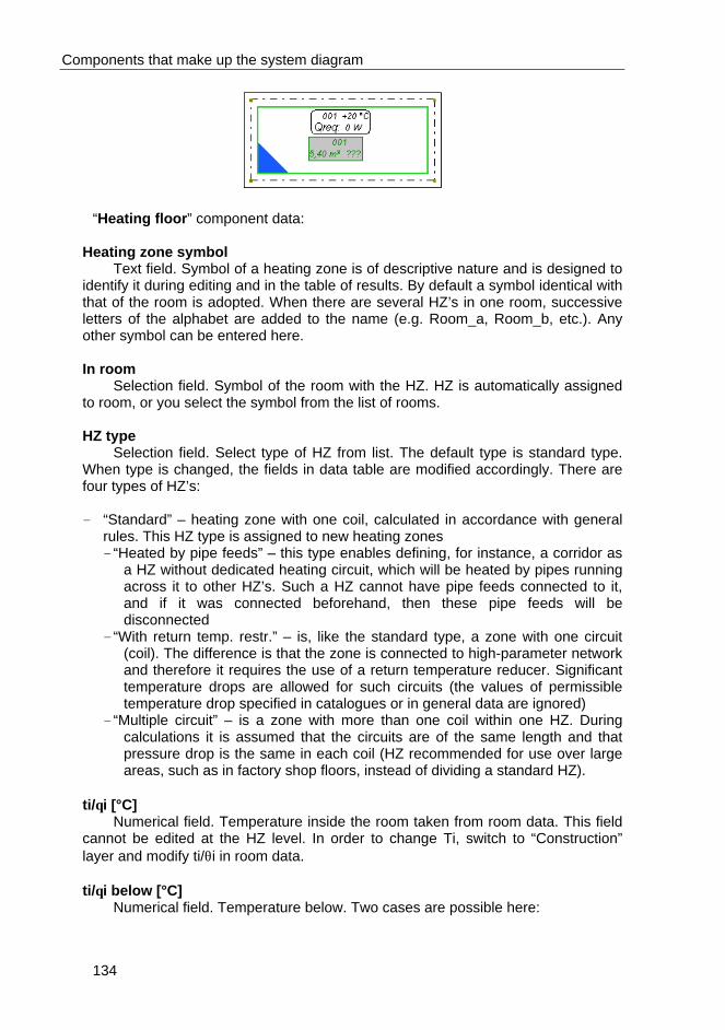
Components that make up the system diagram
134
“Heating floor” component data:
Heating zone symbol Text field. Symbol of a heating zone is of descriptive nature and is designed to identify it during editing and in the table of results. By default a symbol identical with that of the room is adopted. When there are several HZ’s in one room, successive letters of the alphabet are added to the name (e.g. Room_a, Room_b, etc.). Any other symbol can be entered here. In room Selection field. Symbol of the room with the HZ. HZ is automatically assigned to room, or you select the symbol from the list of rooms. HZ type Selection field. Select type of HZ from list. The default type is standard type. When type is changed, the fields in data table are modified accordingly. There are four types of HZ’s: - “Standard” – heating zone with one coil, calculated in accordance with general
rules. This HZ type is assigned to new heating zones - “Heated by pipe feeds” – this type enables defining, for instance, a corridor as
a HZ without dedicated heating circuit, which will be heated by pipes running across it to other HZ’s. Such a HZ cannot have pipe feeds connected to it, and if it was connected beforehand, then these pipe feeds will be disconnected
- “With return temp. restr.” – is, like the standard type, a zone with one circuit (coil). The difference is that the zone is connected to high-parameter network and therefore it requires the use of a return temperature reducer. Significant temperature drops are allowed for such circuits (the values of permissible temperature drop specified in catalogues or in general data are ignored)
- “Multiple circuit” – is a zone with more than one coil within one HZ. During calculations it is assumed that the circuits are of the same length and that pressure drop is the same in each coil (HZ recommended for use over large areas, such as in factory shop floors, instead of dividing a standard HZ).
ti/θi [°C] Numerical field. Temperature inside the room taken from room data. This field cannot be edited at the HZ level. In order to change Ti, switch to “Construction” layer and modify ti/θi in room data. ti/θi below [°C] Numerical field. Temperature below. Two cases are possible here:

Components that make up the system diagram
135
If “ti/θi below” has not been specified in room data, the default value in HZ data is 20 degrees and it can be edited at HZ level. This enables varying of “ti/θi below” in heating zones being part of one room when, for instance, there is a basement under part of the room. If “ti/θi below” has been specified in room data, this value is adopted and cannot be edited at HZ level. To change this value, switch to “Construction” layer and modify “ti/θi below” in room data or delete it (by entering “-“). Qhz/Φhz [W] Numerical field. Part of heat loss in room assigned to given heating zone. (auto) means that this value will be determined automatically by the application when Qrh/Φrh is distributed among HZ’s in the room. If in room data the “Qrh/Φrh distribution ...” field specifies that heat loss is distributed among HZ’s automatically, the contents of the Q/Φ field in HZ data is not editable. Otherwise (when manual distribution of Qrh/Φrh is specified in room) this field can be edited in HZ data: you can specify heat output to be delivered by HZ. Occupied area w/o pipes [m2] Numerical field. Occupied area not covered by floor heating piping, but covered, for instance, by pieces of furniture installed permanently, by a bathtub, or excluded from heating for other reasons. This area reduces the effective area of HZ. Occupied area with pipes [m2] Numerical field. Occupied area covered by RH pipes (e.g. under movable furniture) included as effective area. The percentage of output utilised from such area should additionally be specified. % output utilization of occupied area Numerical field. Percentage of output utilised from occupied area with pipes. Effective area [m2] Numerical field. Effective surface area of HZ – area of floor covered by heating pipes. Value in brackets indicates area determined from the drawing by subtracting strips not covered by heating system along walls and occupied area without pipes. You can specify other value of effective area. Enter “?” to revert to default setting. Area for bill mat. [m2] Numerical field. Surface area for bill of materials. This value (i.e. inclusive of peripheral strips) is taken when drawing up list of materials such as insulation or structural panels. The default value is equal to area of HZ within wall faces. Take notice of this field when effective area is entered manually. This field also enables, when drawing up bill of insulation materials, taking into account the entire surface area of a room where heating pipes (and consequently the HZ) cover only part of it. In such case enter the area of the entire room in place of the value in brackets. Peripheral zone ... Compound field. Enables defining peripheral zone within HZ:

Components that make up the system diagram
136
Radio buttons in the upper part of the window are used to specify whether there is no PZ, or PZ is part of HZ or the entire HZ forms PERIPHERAL zone. If you select the option that PZ forms part of the main circuit, the middle part of the window is activated, where you can specify the edges of HZ occupied by PZ, the width of PZ and the type of PZ: created by compacting pipe laying pattern (cPZ) or forming first part of circuit (connected upstream of OZ – uPZ). The field at the bottom of the window displays the current area of PZ. You can edit the field by entering letter shortcut and pressing the Enter key: “E” – entire HZ forms PZ, “N” – no PZ, “C” – part, by compacting, “U” – part, upstream. Covering Selection field. This field is used to specify the type and heat resistance of floor covering / lining. The resistance of the floor covering is of high importance for radiant heating calculations. Default value in brackets is taken from general data. To specify the required value, you can enter it directly from the keyboard or select one of the preset values displayed after clicking on the button to the right of the field. The contents of the list depend on the selected manufacturer of floor heating system. Floor covering resistance must be within 0 .. 0.15 [(m2 K)/W]. Floor structure ... Compound field. Structure of the floor. You can open a window for automatic definition of insulation options or manual specification of insulation layers:
Components that make up the system diagram
137
In the upper part of the window is a field specifying the floor covering – you can change it here. Below is a field for specifying maximum permissible working load in kN. Below is a field with the total screed thickness (thickness of concrete layer over pipe + pipe diameter + clearance between pipe and insulation). The default value is the minimum thickness of screed taken from catalogue and depends on the fixing system selected and screed type applied. Radio buttons in the middle part of the window are used to switch between automatic (default setting) and manual specifying of insulation option. When manual option is selected, you can select one of the available options displayed on the drop down list or specify individual layers in the table. Up to 3 insulation layers may be specified – structural panel and 2 layers of insulation panels. The field in the lower part of the window displays floor heat resistance indicator and floor thickness. You can modify these values to make allowance for unusual cases. The total floor resistance (in (m2 K)/W), taken for calculations is displayed in the lower right corner of the window. Pipe laying pattern ... Selection field. Specify heating pipe laying pattern in HZ. The specified pattern will be applied during automatic drawing. This field is partly for information purposes, some of the options, however, have an effect on other fields. If “Single meander” option is selected, you cannot use the peripheral zone created by compacting pipe laying (cPZ) – an error message is displayed after launching calculations. Pipe feeds ... [m] Compound field. Displays total length of pipe feeds running across the HZ. You can find a detailed description of the pipe feeds table in section 6.5.3. Label type Selection field. Select from list the type of HZ label in drawing. After selecting “Configure”, a component appearance window is opened, where you can create (by copying) and configure the labels of components in the drawing. After specifying a new label, it is then available in a pull down list in the table. Label on printout Selection field. Switch on/off the printing of the field with HZ label. Max DeltaP [kPa] Numerical field. Maximum pressure drop in HZ. Value in brackets indicates default value taken from general data. Component status Selection field. Select from list the current status of component: existing or under design. Affects only bill of material. Default general data Selection field. You can specify whether the HZ is to use default (standard) general data. Default setting is “Yes”. When “No” is selected, additional fields are displayed in the table, which enable modification of general data:

Components that make up the system diagram
138
You can specify pipe fastening system other than the default system selected in general data, change the type and / or diameter of pipe used, specify pipe laying spacing separately for OZ and PZ and change the restrictions on temperature drop of the medium in the circuit (temperature difference – ∆t/∆θ), also separately for OZ and PZ.
You can also draw the heating floor within a room using the manual drawing
component: “Heating floor (manual)” . In this case the shape of HZ is determined by the user.
♦ There is a function that enables fast arrangement of heating zones. To use this
function, select “Insert HZ to each room” from the “Components” menu or click the
button on the “Radiant” toolbar.
6.2.2. Heating wall
The “Heating wall” component is inserted into “Plan view” type sheets only. When AUTO mode is enabled the heating wall is attracted to the walls in the room.
Button on the “Radiant” toolbar: Appearance on screen (plan view):
“Heating wall” component data:
Heating zone symbol Text field. Symbol of a heating zone is of descriptive nature and is designed to identify it during editing and in the table of results. By default a symbol identical with that of the room is adopted. When there are several HZ’s in one room, successive letters of the alphabet are added to the name (e.g. Room_a, Room_b, etc.).

Components that make up the system diagram
139
In room Selection field. Symbol of the room with the wall. The component is automatically assigned to room, or you select the symbol from the list of rooms. ti/θi [°C] Numerical field. Temperature inside the room taken from room data. This field cannot be edited at the HZ level. In order to change ti/θi, switch to “Construction” layer and modify ti/θi in room data. ti/θi below [°C] Numerical field. Temperature on the opposite side of the heating wall. The default value can be changed by the user. Qhz/Φhz [W] Numerical field. Part of heat loss in room assigned to given heating zone. (auto) means that this value will be determined automatically by the application when Qrh/Φrh is distributed among HZ’s in the room. If in room data the “Qrh/Φrh distribution ...” field specifies that heat loss is distributed among HZ’s automatically, the contents of the Q/Φ field in HZ data is not editable. Otherwise (when manual distribution of Qrh/Φrh is specified in room) this field can be edited in HZ data: you can specify heat output to be delivered by HZ. Occupied area w/o pipes [m2] Numerical field. Occupied area not covered by wall heating piping, but covered, for instance, by pieces of furniture installed permanently or excluded from heating for other reasons. This area reduces the effective area of HZ. Occupied area with pipes [m2] Numerical field. Occupied area covered by RH pipes (e.g. under movable furniture) included as effective area. The percentage of output utilised from such area should additionally be specified. % output utilization of occupied area Numerical field. Percentage of output utilised from occupied area with pipes. Effective area [m2] Numerical field. Effective surface area of HZ – area of wall covered by heating pipes. Value in brackets indicates area determined from the drawing on the basis of wall length and height data in the building structure. You can specify other value of effective area. Enter “?” to revert to default setting. Area for bill mat. [m2] Numerical field. Surface area for bill of materials. This value (i.e. inclusive of peripheral strips) is taken when drawing up list of materials such as insulation or structural panels. The default value is equal to area within faces. Take notice of this field when effective area is entered manually. This field also enables, when drawing up bill of insulation materials, taking into account the entire surface area of the wall where heating pipes cover only part of it. In such case enter the surface area of the entire wall in place of the value in brackets.

Components that make up the system diagram
140
Covering Selection field. This field is used to specify the type and heat resistance of covering. The resistance of the covering is of high importance for radiant heating calculations. Default value in brackets is taken from general data. To specify the required value, you can enter it directly from the keyboard or select one of the preset values displayed after clicking on the button to the right of the field. The contents of the list depend on the selected manufacturer of wall heating system. Covering resistance must be within 0 .. 0.15 [(m2 K)/W]. Wall structure ... Compound field. Structure of the wall. You can open a window for automatic definition of insulation options or manual specification of insulation layers:
In the upper part of the window is a field specifying the covering – you can change it here. Below is a field for specifying the heat transfer coefficient of plaster in W/(m2 K). Below is a field with the total wall thickness. The default value is the minimum thickness of plaster taken from catalogue and depends on the fixing system selected and plaster type applied. Radio buttons in the middle part of the window are used to switch between automatic (default setting) and manual specifying of insulation option. When manual option is selected, you can select one of the available options displayed on the drop down list or specify individual layers in the table. Up to 3 insulation layers may be specified – structural panel and 2 layers of insulation panels. The field in the lower part of the window displays wall heat resistance indicator and its thickness. You can modify these values to make allowance for unusual cases. The total sideways resistance (in (m2 K)/W), taken for calculations is displayed in the lower right corner of the window. tws/θws max. Numerical field. Maximum temperature of wall surface. Label type Selection field. Select from list the type of surface label in drawing. After selecting “Configure”, a component appearance window is opened, where you can create (by copying) and configure the labels of components in the drawing. After specifying a new label, it is then available in a pull down list in the table.

Components that make up the system diagram
141
Label on printout Selection field. Switch on/off the printing of the field with heating wall label. Max DeltaP [kPa] Numerical field. Maximum pressure drop across heating wall. Value in brackets indicates default value taken from general data. Component status Selection field. Select from list the current status of component: existing or under design. Affects only bill of material. Default general data Selection field. You can specify whether the wall is to use default (standard) general data. Default setting is “Yes”. When “No” is selected, additional fields are displayed in the table, which enable modification of general data:
You can specify pipe fastening system other than the default system selected in general data, change the type and / or diameter of pipe used, specify pipe laying spacing and change the restrictions on temperature drop of the medium in the circuit (temperature difference – ∆t/∆θ).
6.2.3. Manifold
Radiant heating manifold differs from that used in radiator heating systems. Radiant heating system designed by the program does not have to include a manifold only in case of a co-current system or when a circuit with return temperature restriction is used.
Manifolds used in radiant heating must be associated with equipment catalogues.
Button on the “Radiant” toolbar: Appearance on screen (plan / schematic view):
“Manifold” component data:

Components that make up the system diagram
142
Symbol Text field. The symbol is defined automatically, when the manifold in the drawing is within a room, or it can be specified by the user. The symbol is used to identify the manifold when editing data and in the tables of results. No. of outlet pairs Numerical field. Number of spare ports, which may be used later. These are not accounted for in calculations. When, for instance, only radiant heating calculations are done, they may be treated as designed for connecting additional radiators not included in the given project. This enables specifying in the bill of materials a manifold with the number of outlets greater than the number of connected heating circuits. of that spare Numerical field. Number of spare ports, which may be used later. These are not accounted for in calculations. In case of radiant heating calculations, they may be treated as designed for connecting additional radiators. This enables specifying in the bill of materials a manifold with the number of outlets greater than the number of connected heating circuits. Type Selection field. Manifold type selected from catalogue. If “(default)” is specified, then the type specified in general data ia adopted. If a manifold with control elements is selected, valve data are displayed in the table below the manifold data. Supply/return arrangement Selection field. The position of the supply part of the manifold in relation to the return part (for angle of 0°). This only has an effect on the drawing and enables the adaptation of the manifold drawing to the actual arrangement of the supply and return parts of the manifold. Opposite arrangement of the parts of the manifold may result in the crossing over of pipes in the drawing. Cabinet type Selection field. Select cabinet type from catalogue. If “(default)” is specified, then the type specified in general data is adopted. Cabinet axis above floor [m] Numerical field. Distance between cabinet axis and the floor. The required number of pipes to construct vertical route will be accounted for in the bill of materials. Show RH data Selection field. Here you can change the display of additional RH data in the table. The default setting is “No”. When you enter “Yes”, additional data fields appear in the table. ∆t/∆θ min OZ Numerical field. Minimum temperature drop for HZ in occupied zone. ∆t/∆θ max OZ Numerical field. Maximum temperature drop for HZ in occupied zone.

Components that make up the system diagram
143
∆t/∆θ min PZ Numerical field. Minimum temperature drop for HZ in peripheral zone. ∆t/∆θ max PZ Numerical field. Maximum temperature drop for HZ in peripheral zone. Max DeltaP [kPa] Numerical field. Maximum pressure drop in HZ. Component status Selection field. Select from list the current status of component: existing or under design. Affects only bill of material. Draw label Selection field. Specify whether the component label is to be drawn in the sheet. Then manifold symbol appears in the drawing. The default setting is “No”. Valves other than std. Selection field. Manifold valves are not independent components; they constitute manifold fittings. Depending on manifold type, valves may be indicated – when they are factory-mounted on the manifold. When the field is set to “No”, then the factory-mounted valve is adopted in calculations. If “Yes” is specified, then during calculations a valve matching the flow rate is sized within the range applicable to the manifold. Supply valve ... Selection field. For selecting valve type placed on the supply end. Ret. valve ... Selection field. For selecting valve type placed on the return end.
6.2.4. Mixer (temperature reducer)
This component represents a mixer (temperature reducer) used to connect floor heating systems.
Button on the “Radiant” toolbar: “Mixer” component data same as in section 6.1.15.
6.2.5. Pipe feed and pair of pipe feeds
Pipe feeds in the program are used for connecting heating zones to manifolds. Although in reality a pipe feed forms with the heating circuit one segment of piping, in the application it constitutes a separate component. This is justified by the specific nature of the pipe feed: it reduces the surface area available to circuits in rooms which the pipe feed passes and gives up heat to those rooms (unless it is insulated). The designer must see to that the documents clearly specify planned manner of laying out

Components that make up the system diagram
144
pipe feeds from manifolds to heating zones, and at the same time pipe feeds must be appropriately taken into consideration when doing calculations.
Pipe feeds are edited in a similar manner to pipe-runs in the graphical editor. A pair is available as well as a single pipe feed, which takes on the role of a supply or return line, depending on connection point. Pipe feed pair is a single component only at the time of placing it in the drawing. Later the supply and return pipe feeds form separate components, which can be edited independent of each other.
Buttons on the “Radiant” toolbar: Appearance on screen (plan) (colours: red = supply, blue = return):
“Pipe feed” component data:
Length Information field. Total length of pipe feed. This value may be taken from drawing or may be the result of adding the lengths of fragments of pipe feed, if the length was imposed manually. Across HZ ... Compound field. Button on the right side of the field enables display of table with data on the crossing by pipe feeds of individual HZ’s. Detailed description of the manner of editing this table is given in section 6.5.3.
Line style Selection field. Select from list the appearance of the pipe feed or configure it – component appearance window is opened. “Pipe feed pair” data during drawing: There is no need to change any data associated with pipe feeds. However, two options of pipe feed data configuration are recommended:

Components that make up the system diagram
145
Retain default settings Spacing (auto) and non-insulated pipe feeds. In this case the HZ across which the pipe feeds run is ‘simulated’. In the case of HZ heated by pipe feeds that pipe spacing will be adopted, which matches heat requirements of that HZ. User-specified spacing – (preferably small, e.g. 10 cm) and insulated pipe feeds. Pipe feeds are arranged close to each other and are insulated to eliminate heat dissipation. If insulation is not provided on pipe feeds arranged close to each other, substantial floor overheating may occur in HZ’s with, for instance, ceramic tiles and pipe spacing in the main circuit of e.g. 30 cm.
6.2.6. Radiant heating circuit
A radiant heating circuit can only be inserted into a “Schematic view” type sheet. RH project calculations are not done for this component. As a shadow it may have results assigned from the calculated original HZ or may have flow resistance and rate values specified by the user. In calculations the floor heating circuit is treated as a terminal unit with specified pressure and temperature drop. It is distinguished for identification in the drawing and, if necessary, for appending results of floor heating calculations executed with other program. These results may also be entered directly into terminal unit data.
Button on the “Radiant” toolbar: Appearance on screen (schematic view):
“Circuit” component data:
Room symbol Text field. Room symbol – text describing the room. Circuit symbol Text field. Floor heating circuit symbol. You can select it from the list, provided that the floor heating calculation results file has been loaded (in case of Instal-therm without the RH calculations feature). Type Selection field. Specify whether the heating circuit applies to floor heating or wall heating. After selection, the appearance of the component in the drawing is changed accordingly. Q/Φ of terminal unit [W] Numerical field. Required output of terminal unit.

Components that make up the system diagram
146
Supply temp. [°C] Numerical field. Supply temperature in the circuit. You can specify value other than default. ∆t/∆θ [°C] Numerical field. Specified temperature drop across terminal unit. Value in brackets is default value. Circuit press. drop [kPa] Numerical field. Pressure drop across heating circuit. Water capacity [dm3] Numerical field. Water capacity. H [m] Numerical field. Elevation of terminal unit. It can be determined automatically (value in brackets) or specified by the user. To revert to automatic determination enter “?”. Component status Selection field. Select from list the current status of component: existing or under design. Affects only bill of material. Label type Selection field. Select from list the type of circuit label in drawing. After selecting “Configure”, a component appearance window is opened, where you can create (by copying) and configure the appearance of components in the drawing. After specifying a new label, it is then available in a pull down list in the table.
6.2.7. Floor heating manifold
A floor heating manifold represents the entire manifold of floor heating system with circuits. It is presented in the drawing in a schematic way.
The floor heating manifold with heating circuits and the floor heating manifold with mixing pump and heating circuits may only be inserted into a “Schematic view” type sheet.
RH project calculations are not done for this component. As a shadow it may have results assigned from the calculated original HZ or may have flow resistance and rate values specified by the user. In calculations the floor heating manifold is treated as a terminal unit with specified pressure and temperature drop. It is distinguished for identification in the drawing and, if necessary, for appending results of floor heating calculations executed with other program. These results may also be entered directly into terminal unit data.
Buttons on the “Radiant” toolbar: Appearance on screen (schematic view):

Components that make up the system diagram
147
“Floor heating manifold” component data:
Room symbol Text field. Symbol of room where the manifold is installed. Floor heat. manifold symbol Text field. Symbol of a floor heating manifold. You can select it from the list, provided that the floor heating calculation results file has been loaded (in case of Instal-therm without the RH calculations feature). Q/Φ of terminal unit [W] Numerical field. Required output of terminal unit. Supply temp. [°C] Numerical field. Supply temperature of the manifold. You can specify value other than default. ∆t/∆θ [°C] Numerical field. Specified temperature drop across terminal unit. Value in brackets is default value. Circuit press. drop [kPa] Numerical field. Pressure drop across manifold and floor heating circuits. Water capacity [dm3] Numerical field. Water capacity. H [m] Numerical field. Elevation of terminal unit. It can be determined automatically (value in brackets) or specified by the user. To revert to automatic determination enter “?”. Component status Selection field. Select from list the current status of component: existing or under design. Affects only bill of material. Label type Selection field. Select from list the type of manifold label in drawing. After selecting “Configure”, a component appearance window is opened, where you can create (by copying) and configure the appearance of components in the drawing. After specifying a new label, it is then available in a pull down list in the table.

Components that make up the system diagram
148
6.2.8. Polylines for depicting piping
Polylines for drawing pipe system is a graphical component designed to depict part or the whole of pipe system within a heating zone. Their properties are the same as those of an ordinary polyline. Piping can be drawn automatically or manually.
How this line can be used to draw pipe systems is explained in section 0. These components are only available on a “Plan view” type sheet in the “Floor heat. dwg.” layer in the “Radiant” tab.
Buttons on the “Radiant” toolbar: Appearance on screen (plan view) (colours: red = supply, blue = return):
“Polylines for depicting piping” component data:
! Pair of polylines has specific data fields, which are used only when polylines are placed in the drawing and apply to their relative position and spacing. After placing a pair of polylines, each of them forms a separate component and has other fields in the table.
Fields used when placing a pair of polylines in the drawing:
Pipe spacing Numerical field. Pipe spacing for a pair of polylines. When AUTO mode is enabled, the spacing is automatically adjusted to the value read from the results for the HZ. Relative arrangement s/r Relative arrangement of supply and return for a pair of polylines. When AUTO mode is enabled, the relative arrangement of lines is adjusted automatically depending on the situation on the drawing.
Fields displayed when marking a polyline drawn before: Line style Selection field. Select from list the appearance of the line or configure it – component appearance window is opened.

Components that make up the system diagram
149
6.3. Inserting and editing heating zones (HZ’s)
6.3.1. Pasting a HZ with a spacing from walls
The first stage of editing a radiant heating system is the indication of the rooms where radiant (floor or wall) heating is to be used. This is done by pasting heating zones into these rooms.
♦ To paste a heating floor into a room:
1. Select a “Heating floor” component by clicking on the button on the “Radiant” toolbar. The heating zone insertion mode is enabled.
2. Move the mouse pointer to the room where you want to paste the HZ. 3. Press the left mouse button. The HZ is pasted into the room. By default it
spreads over the entire area of the room leaving out a spacing from external and internal walls defined in general data. A HZ label in a box also appears. Later, when you want to mark the HZ, click this box.
4. To modify the size and shape of the inserted heating floor, right click the HZ label and select “Change type to freely modifiable” from the pop up menu. Handles appear in the corners of the HZ, which you can move by left clicking and dragging.
5. You can also draw the heating floor within a room using the manual drawing
component: “Heating floor (manual)” . In this case the shape of HZ is determined by the user.
♦ There is a function that enables fast arrangement of heating zones. To use this
function, select “Insert HZ to each room” from the “Components” menu or click the
button on the “Radiant” toolbar.
♦ To paste a heating wall into a room:
1. Select a “Heating wall” component by clicking on the button on the “Radiant” toolbar. The heating zone insertion mode is enabled.
2. Move the mouse pointer to one of the walls in the room where you want to paste the HZ. If the AUTO mode is enabled, the inserted wall is attracted to the walls in the room.
3. Press the left mouse button – one end of the wall is inserted. Move the pointer to the point where you want to place the other end of the wall and press the left mouse button. To complete wall insertion, press the right mouse button. A HZ label in a box appears. Later, when you want to mark the HZ, click this box.
! Definition: the spacing between HZ and wall is the spacing between the
conventional boundary of HZ and the wall face. The conventional boundary of HZ runs along the outermost pipe at a distance of half of pipe spacing. For instance, if the pipe spacing is 20 cm and the distance between HZ and wall is 15 cm, then the outermost pipe should run 15 + ½ * 20 = 25 cm from the wall.

Components that make up the system diagram
150
The default spacing depends on manufacturer’s guidelines. Note that proper specification of spacing is very important as it has an impact on the effective heating zone. For instance, in a room 4 x 5 m and “gross” surface area of 20 m2, the rejection of a 15 cm wide strip along the walls reduces the heated area by ca. 2.6 m2, which corresponds to ca. 13%!
Proper handling of the spacing consists not only in following the manufacturer’s
guidelines in this aspect, but also in ensuring proper realisation of the heating circuits in this aspect. Error may be caused either by not taking into account the spacing in the calculations and implementing that spacing in the construction of the heating system (overstated area of HZ in calculations), or by taking it into account in the calculations and not implementing it in the construction (understated area of HZ in calculations). It is therefore essential that all assumptions made at the stage of calculations be put into practice.
6.3.2. Dividing a HZ
If there is a need to have several HZ’s (heating circuits) in one room, the existing HZ must be divided into the corresponding number of parts. There may be various reasons for having several HZ’s in one room. However, it is not advisable to divide HZ’s before making calculations, even when it is clear that division is necessary. This may lead to the creation of a wrong number of circuits (HZ’s) and the need to introduce a new HZ into the room and to divide it again.
The reason for that is the adopted methodology of making several calculations and modifications of the system. After the first calculations the error list displays messages regarding the recommended division of HZ’s that would meet all requirements (pipe lengths, pressure drops, flow rate). If you divide a HZ before calculations into, say, 3 parts, and then calculations indicate that the HZ has to be divided into 5 parts, you have to insert and divide a HZ again.
! The current version of the application does not allow combining heating zones
that have been divided. If the division made is wrong, use the “undo” function, and if this is not possible, the HZ’s existing in the room have to be removed and a new HZ must be inserted and divided.
There are two methods of dividing heating zones: using the pop-up menu or the
function of dividing HZ in any proportion. The line of division may be vertical or horizontal. The division may be made “without joints” (several HZ’s within one floor zone) or “with joints” (division into separate circuits that form at the same time separate concrete slabs). The presence or absence of joints has no effect on calculations, it is however important from the structural point of view. Joints must be used in accordance with manufacturer’s guidelines, taking into account both the maximum permissible surface area of floor zones and their desired shape.
The current version of the application does not check the correctness of the floor
structure. Attention must be paid to make appropriate HZ divisions “with joints”, so that joints are properly arranged in the printout and proper number of expansion strips is determined.
Dividing HZ using pop-up menu commands

Components that make up the system diagram
151
Using the pop-up menu is fast and simple. It allows dividing a HZ into 2, 3, 4 or more new HZ’s.
♦ To divide an existing HZ using the pop-up menu:
1. Position the mouse pointer on the label of the heating zone to be divided. 2. Click the right mouse button. The pop-up menu of the HZ is displayed (the left-
hand list in the figure below). Move the pointer to the first command “Divide heat. zone ...”. The division menu is displayed (the right-hand list in the figure below):
3. After selecting the desired option, click the mouse button. The heating zone is divided into the indicated number of parts. The zone is divided into parts equal with respect to their dimension in the vertical and horizontal axis (depending on the type of division made).
Dividing HZ with the use of HZ dividing function
The heating zone dividing function enables dividing a HZ in any selected point,
both vertically and horizontally, with a joint or without a joint. The HZ is always divided into 2 parts. To acquire more parts the dividing operation has to be repeated.
♦ To divide an existing HZ using the HZ dividing function:
1. Select “Components / Divide components” (Ctrl+Q), to divide without a
joint or “Components / Divide heating surface (free) with expansion joints” to divide with a joint.
2. When the AUTO mode is enabled the mouse pointer is attracted to the surface. Mark the starting point of the division line by pressing the left mouse button.
3. Now move the mouse pointer to the other end of the division line. If the line is attracted in an undesired way in the AUTO mode, you can press and hold the Shift key and press the left mouse button followed by the right mouse button. The HZ is divided.

Components that make up the system diagram
152
In the result of dividing a heating zone with the use of any of the described
methods new HZ’s are formed, which constitute separate components. By default the new HZ’s are named <Room_name>_a, <Room_name>_b and so on and they acquire all data from the original HZ, except for peripheral zone forming part of the HZ. If the original HZ was connected to the heating system, the pipe feeds and the new HZ will be disconnected. To reconnect click on the disconnected pipe feeds. Pipe feeds to the other new HZ’s must be arranged.
! When dividing a HZ, the data on the peripheral zone (PZ) that forms part of the
original circuit (uPZ or cPZ) are lost. This is because of the ambiguity of these data after the division. Therefore care must taken to restore the PZ data.
6.3.3. HZ that covers only part of room
By default the heating zone covers the entire area of the room. This facilitates editing in usual cases. In unusual cases you can divide the HZ and remove those HZ’s, which are not necessary or you can using a non-standard spacing between HZ and the wall or draw HZ’s in the room manually.
♦ To create a HZ that covers only part of room:
1. Insert the HZ into the room (see 6.3). 2. Divide the original HZ in such manner that one of the new HZ’s covers the area
intended to be eventually covered by floor heating, for example:
3. Delete the unnecessary HZ’s:

Components that make up the system diagram
153
The method described enables creating any HZ with the shape of a convex
polygon. In less complex situations, when it is sufficient just to move the HZ border away from the wall, you can use another method consisting in specifying a non-standard spacing of HZ from the wall.
♦ To move the border of HZ away from the selected partition:
1. In the project options (F7) in the “Radiant heating – floor heating” tab specify standard spacing of HZ from external and internal walls.
2. To specify a non-standard spacing for one of the walls, select the “Construction”
layer and mark the wall from which a non-standard spacing of HZ is to be retained.
3. Specify the distance between HZ and wall in the “Spacing from wall” field. HZ area will be modified accordingly:

Components that make up the system diagram
154
It is advisable to specify appropriate distances from walls before inserting heating
zones into the rooms and editing them (e.g. dividing). If you change the distance between HZ and wall in rooms where HZ’s have already been inserted, the latter can be modified incorrectly, particularly in complex cases where several HZ’s border with one wall.
In a situation where the area not covered by heating is fragmentary and
haphazard, use the “Occ. area w/o pipes [m2]” field in the HZ data and enter the desired value. To place the occupied area fragments in the drawing use graphical components and labels.
♦ To draw a HZ in a room manually:
1. Select “Heating floor (manual)” 2. Move to the drawing area and mark the first corner of the heating zone by
pressing the left mouse button:
3. Insert all corners of the HZ to form desired shape. To finish inserting, press the right mouse button:
This method enables inserting heating zones of any shape and size.
! The quantity of materials for heating zones of any shape is calculated for the area covered by that HZ. Therefore such zones should be used in special cases only.

Components that make up the system diagram
155
6.4. Inserting manifolds and manifold fittings
The second step in editing the system is placing manifolds on the drawing. The number of manifolds depends on the number of HZ’s and the designer’s intentions: it may, for instance, be advantageous to divide one large manifold into two smaller ones in order to reduce the total number of pipe feeds in the system.
After making calculations it may be necessary to divide some of the HZ’s. This requires provision of additional manifolds or, more often, addition and adaptation of outlet ports to existing manifolds. Appropriate functions are available to facilitate these operations.
♦ To place a manifold in the drawing and adapt it to the construction:
1. Select “Manifold” component by clicking the button on the “Radiant” toolbar. The manifold inserting mode is enabled.
2. Position the mouse pointer at the point where you want to place the manifold and press the left mouse button – the manifold is placed on the drawing. The manifold may be located anywhere. For technical reasons, however, it should be placed near or inside a wall:
3. The small square with an arrow enables rotating the manifold in the drawing:
4. Move the manifold so that it is contiguous with the wall: inside the room (surface-mounted cabinet) or inside the wall (concealed cabinet):
. To add fittings (manifold valves) to the manifold you must specify their type. In the
description of inserting a manifold above, there was no default manifold type defined in the general data. In this case the manifold inserted is “clean” – i.e. with no type and fittings specified. If the manifold type is specified, default fittings for the given type of manifold will be placed on its inlet and outlet sides, and new fields corresponding to the fittings will appear in the manifold data table:

Components that make up the system diagram
156
Depending on the type of manifold, the valves may be defined unambiguously –
factory-mounted. When the “Valves other than std.” field is set to “No”, then the factory-mounted valve is adopted in calculations. If “Yes” is specified, then during calculations a valve matching the flow rate is sized within the range applicable to the manifold.
It is not necessary to determine the required number of outlets in the manifold
being inserted, as the necessary outlet will be added when subsequent pipe feeds will be connected.
A different procedure must be applied when you want to add ports to an existing manifold that has pipe feeds already connected to it. Simple increasing of the number of ports causes addition of ports at the end of the manifold. Sometimes, however, to avoid crossing of the pipe feeds, you may want to insert an additional port between, for instance, existing ports numbers 2 and 3. There are two ways to go about that. You can add a port at the end of the manifold and reconnect some of the pipe feeds to make a port available in the required position or you can insert the port in the required position and make the necessary graphical corrections of the components that were shifted. The latter method is simpler and preferred.
♦ To insert additional ports in the desired positions of the manifold:
1. Mark the manifold by left clicking on it within an area without pipe feeds. 2. With the pointer positioned on the manifold, press the right mouse button to
display the manifold pop-up menu and select the first item in the menu: “Insert connection point ...”:
3. A menu is displayed, shown on the right side in the figure above. Select the required item. The first port is designated as “1”.
4. After selecting one of the options, the new connection is inserted accordingly. The existing ports are automatically drawn aside. This, however, may deform some of the pipe feeds, which will then require correcting:

Components that make up the system diagram
157
6.5. Editing pipe feeds
6.5.1. Inserting pipe feeds in the drawing
After placing heating zones and manifolds in the drawing you can proceed with arranging pipe feeds. The routes of pipe feeds should resemble the actual layout of the system. This makes the drawing more useful as an aid in constructing the system and improves the accuracy of calculations.
It is advisable to draw pipe feeds from the manifold to the heating zone, not the
opposite direction. In all usual cases, when the supply pipe feed runs parallel to the return line, a pipe feed pair should be used. The AUTO and ORTO modes are also helpful.
Before editing pipe feeds plan the assignment of manifold ports to individual HZ’s to avoid crossings.
When a HZ is being automatically connected to the manifold, by default the first leftmost unoccupied port of the manifold is taken and the pipe feed is connected to it. You can change this setting when drawing pipe feeds: in the “Manifold outlet no.” field in the data table indicate the “any” option instead of “first free” or specify a number of outlet pair. Then the pipe feed can be connected to any port or, when outlet number has been specified, the pipe feed will be automatically connected to that outlet.
♦ To link a HZ to a manifold using a pipe feed: 1. Select appropriate viewing scale. The optimum scale is such, that enables
distinguishing the individual ports of the manifold and existing pipe feeds and at the same time displays the entire area across which the pipe feed should be laid.
2. Select the “Pipe feed pair” component by clicking on the button on the “Radiant” toolbar. The mode of inserting a pipe feed pair is enabled.
3. Position the mouse pointer on the manifold at the point where the port for the pipe feed is located. In the AUTO mode crosses indicate the port to which the pipe feed will be connected:

Components that make up the system diagram
158
4. Press the left mouse button. The pipe feed is connected to the manifold. The mode of inserting a pipe feed (its first segment) remains enabled. Each subsequent single click of the left mouse button inserts a point of bend of the pipe feed. The current route of the pipe feed, which depends on the current position of the mouse pointer, is represented by a grey line:
5. To complete editing the pipe feed you have to connect it to the HZ. Position the mouse pointer on the border of the HZ to be connected. In the AUTO mode suggested points of connection are displayed: a all you have to do is press the left mouse button: the pipe feed is connected to the HZ and the mode of selecting is enabled
6. If the AUTO mode is disabled, you have to position the mouse pointer on the edge of the HZ exactly at the desired point and then press first the left mouse button (to connect the pipe feed to the HZ) followed by the right mouse button (to complete connecting and enable the mode of selecting).
Making connections with the AUTO mode disabled may be necessary when in the
AUTO mode the last segment of the pipe feed is placed incorrectly. The best solution in this case is to disable temporarily the AUTO mode by pressing the Shift key and make the connection.
A pipe feed may consist of any number of segments (in the drawing). These
segments may be connected by means of an empty diamond symbol, which indicates a point of bend, or by means of a solid square symbol, which indicates a point of connection of pipe feeds (connection in the drawing, not in real terms) – a pipe feed with a solid square in the middle is treated by the program as two separate pipe feeds. This is admissible and has no effect on calculation results, but it makes editing of pipe feed data more difficult (one real pipe feed is divided into several parts which results in more rows in the pipe feed data table). If this situation occurs, use the function of combining pipe feeds (see next item).

Components that make up the system diagram
159
Note the difference between the spacing between pipes in a pipe feed pair in the drawing and the actual spacing that is taken into account in calculations. When using the pipe feed pair component, they are drawn spaced apart at a distance. You can change the pipe spacing in data table when inserting a pipe feed - that distance, however, is not taken into account in calculations.
The actual distance between pipe feeds adopted for calculations may be specified by the user (in the data table in the field “Across HZ ...”) or it can be determined by the program. This, however, does not change the spacing in the drawing after calculations!
The length of the entire pipe feed and lengths of its fragments running across
individual HZ’s are taken from the drawing – no matter how many segments there are in the drawing.
! Pipe feeds cannot be branched.
! Before making calculations, the program checks connections in the system.
Therefore there should be no unconnected HZ’s or “blind” pipe feeds. Each HZ requires two connection points – for the supply pipe feed and the return
pipe feed. One exception is a HZ heated by pipe feeds - it has no connection points.
6.5.2. Modifying existing pipe feeds
Sometimes it is necessary to modify an existing pipe feed. If the pipe feed is short and consists of several segments, it is better to remove existing segments and draw a new pipe feed. In the case of longer pipe feeds, or those, which require much editing, modification may be necessary. The graphical editor provides a set of functions that enable modifying existing pipe feeds. These functions become available after selecting the “Components / Pipe-run menu” command or after right clicking on the selected pipe feed:
The pipe feed menu includes the following functions:
- add point, - delete point, - divide pipe feed into two, - combine two pipe feeds into one, - disconnect.

Components that make up the system diagram
160
The manner of using these functions and examples of pipe feed modifications
made with the use of these functions are described below.
♦ To add a new point on one of the segments of a pipe feed: 1. Mark the selected segment of the pipe feed. 1. Select “Components / Pipe-run menu / Add point”. 2. A new point is added in the middle of the marked segment.
♦ To delete a point (empty diamond symbol) on a pipe feed:
1. Mark the selected point. 1. Select “Components / Pipe-run menu / Delete point” or select “Edit / Delete
point” (Del). 2. The marked point is deleted. If the segments of the pipe feed that were joined by
this point did not form a straight line, a new segment connecting points adjacent to the deleted point is formed..
♦ To combine two pipe feeds (in the drawing) into one:
1. Mark the connection point of the two pipe feeds (solid square symbol). 1. Select “Components / Pipe-run menu / Combine pipe-run into one”. 2. Pipe feeds are combined into one.
♦ To divide a pipe feed into two separate pipe feeds (in the drawing):
1. Mark the selected internal point or selected segment of pipe feed. 1. Select “Components / Pipe-run menu / Divide pipe-run into two”. 2. The pipe feed is divided into two pipe feeds connected in the indicated point or
in the centre of the indicated segment of pipe feed.
♦ To disconnect a pipe feed: 1. Mark the point of connection of the pipe feed with other component (HZ,
manifold or other pipe feed) or the fragment of pipe feed ending at that point or on the entire pipe feed.
1. Select “Components / Disconnect” (Ctrl+R, ) or “Components / Pipe-run menu / Disconnect”.
2. The components are disconnected – the small solid square symbol is replaced by a large empty diamond symbol. If the entire pipe feed (all its segments) was marked in the first step, it will be disconnected at both ends.
Examples of pipe feed operations:
♦ To “move” the pipe feed towards the wall on the drawing:
1. Initial situation:

Components that make up the system diagram
161
2. To isolate the part of pipe feed to be moved towards the wall, execute the “Add point” command four times: execute the command once, mark one of the new segments and execute the command again and so on. The following result should be achieved:
3. Move the bend points to appropriate locations (prior to that disable the ORTO mode, if it was enabled). Individual segments of the pipe feed are modified accordingly:
4. Modify the return pipe feed in the same way.
♦ To introduce several heating meanders in a HZ across which runs a pipe feed: 1. Initial situation:
2. Disconnect the existing pipe feeds from the HZ and move their terminal points to the point where the meanders should start. This can be done by carrying out the operation of disconnecting pipe feeds from the HZ and then moving their terminal point, or directly – when you move the terminal point of pipe feed it will be automatically disconnected from the HZ, as the latter cannot be moved. The following result should be achieved:

Components that make up the system diagram
162
3. Insert the missing part of the pipe feed:
4. Combine the pipe feeds created in the drawing into one:
6.5.3. Pipe feed data table (as part of HZ table)
The pipe feed data table displays data of individual fragments of the pipe feed, a fragment being the part of pipe feed that runs across a HZ, and not a segment in the drawing:
The data table always consists of the same data fields (columns), apart from that,
depending on the situation, it includes or not the fields “Across HZ” and “To HZ”, whereas the contents of the data table (rows) depend on the location from which it was called:
- Room – when you open the data table in a room, all fragments of pipe feeds running across the HZ assigned to that room will be displayed in the table.

Components that make up the system diagram
163
- HZ - when you open the data table within a heating zone, all fragments of pipe feeds running across the HZ will be displayed.
- pipe feed – when you open the data table on a pipe feed, all fragments of that pipe feed running across various HZ’s will be displayed.
On account of the above, data of a fragment of a pipe feed can be modified after
marking either the pipe feed itself, or the HZ or room across which that fragment of pipe feed runs. Supply pipe feeds are described in red, return pipe feeds – in blue. After clicking on the selected row in the “Across HZ” or “To HZ” column, the pipe feed is highlighted in the drawing in yellow.
The data table includes the following fields:
Across HZ ... Identification of the fragment of pipe feed: name of the HZ across which it runs. This field is displayed in the data tables of room and of pipe feed. In the case of HZ data table, all fragments of pipe feeds included in it run across that HZ. This field is not editable. After clicking on the selected row in the “Across HZ” or “To HZ” column, the pipe feed in the drawing is highlighted in yellow. To HZ Identification of the fragment of pipe feed: name of the HZ to which it runs. This field is displayed in the data tables of room and of HZ. In the case of pipe feed the information to which HZ it (and all its fragments) runs is displayed in a separate field of the pipe feed data table. This field is not editable. Length Length of the fragment of pipe feed. The default value (taken from the drawing) is enclosed in brackets. The length of pipe feed taken from the drawing does not include those its fragments that run outside of any HZ! In usual cases this means that short segments of the pipe feed that, for instance, run across a door, are neglected. This is not a source of any significant error. However, situations where a pipe feed runs in the strip between a wall and a HZ should be avoided, as that fragment of the pipe feed will not be assigned to any HZ and will be omitted in heat calculations. You can overwrite the value in the field. This is necessary when the actual length of a pipe feed differs form the length taken from the drawing (an alternative is to change the route of the pipe feed in the drawing in such a way as to achieve the length taken from the drawing equal to the actual length). Insul. Insulation of the fragment of pipe feed – a selection field, where you can specify whether the fragment is not insulated (default value – “N”), is laid in conduit (“P”) or insulated (“I”). Insulation properties selected in case of “I” depend on the manufacturer and are specified in the catalogue. Note that the conduit itself has no significant insulating properties and it is used for protection and has an effect on the bill of materials, but does not reduce the heat output of the pipe feeds. Pipe spacing Here you can determine the pipe spacing for calculations for the given pipe feed fragment. The spacing values available are those for the HZ across which that
Components that make up the system diagram
164
fragment of pipe feed runs and an (auto) option, which is the default setting. The pipe feeds spacing should be treated as a strip of floor of the width equal to the spacing in the axis of which the pipe feed runs. If “N” or “P” is selected in the “Insul” field, then (auto) means that the pipe spacing for that fragment of the pipe feed will be equal to that of the HZ across which it runs, in other words it will simulate that HZ. Such a solution is favourable from the technical point of view. However, it may cause that individual fragments of one pipe feed running across different HZ’s will be arranged with various spacing. If this may cause some concern during construction, you can specify a uniform spacing for all fragments of the pipe feed. If “I” is selected in the “Insul” field, then (auto) means that the pipe spacing for that fragment of the pipe feed will be the minimum available spacing. % util. Percentage of utilisation of the output of the fragment of the pipe feed. Default setting – 90%. This field determines what part of the heat output of the pipe feed fragment is taken for calculations. For instance, if the output of the pipe feed is 130 W, and the setting in the field is 50%, then the effective output is 65 W and that value is deducted from the required output of the HZ across which that fragment of the pipe feed runs. In practice this field reflects the relative levels of usage of the room to which the pipe feed runs and of the room across which the pipe feed runs. In reality, the pipe feed provides either 100% of output (when the terminal HZ is switched on) or 0% (when the terminal HZ is switched off). If the level of usage is high, you can enter even 100% of output utilisation. If the level of usage is low, the percentage should be reduced to less than 50.
6.5.4. Pipe feeds in HZ’s heated by pipe feeds
Situations are also accounted for when the HZ (room) is heated only by pipe feeds – there is no separate heating circuit. There may be various causes of such situations:
1. There are so many pipe feeds that run across the room, that there is no need or possibility to insert a separate circuit there. This applies mainly to small rooms where manifolds are installed, e.g. entrance hall, corridor.
2. The room is so small that placing a separate circuit there would make adjustment of the system impossible, as its flow resistance would be too low. This applies mainly to bathrooms, toilets, etc.
HZ heated by pipe feeds with many pipe feeds running across
Example of a HZ heated by pipe feeds with many pipe feeds running across:

Components that make up the system diagram
165
The situation presented above is very common: most often manifolds are installed
in entrance halls or corridors. Often these rooms are small and the heat loss there may not be high. The remainder of the heat loss may also be distributed among adjacent rooms in a situation when HZ heated by pipe feeds would not cover that loss.
From the editing point of view it is important that there are so many pipe feeds running across in relation to the surface area of the room, that they cover large part of it even if the routes of pipe feeds are the shortest possible. It is advisable then to select (auto) in the pipe spacing field – uniform pipe spacing is suggested that provides best heat output results. If in all variants overheating in the HZ occurs, some pipe feeds must be insulated.
HZ heated by pipe feeds in small rooms
Example of a HZ heated by pipe feeds in a small room (view in the print layer):
An often applied method of heating a small room, such as a toilet, is to place a
heating circuit connected in series to another heating circuit, preferably one that heats another small room.
In the current version of the program it is not possible to connect HZ’s in series. However, such situation may be accounted for by appropriate application of HZ’s heated by pipe feeds. The circuit (loop) in the toilet connected in series may simply be treated as part of a pipe feeds running to the “terminal” HZ, as shown in the figure.
It may be advisable, for the sake of calculations, to specify exactly the pipe spacing and pipe laying pattern in the drawing and to specify the same spacing for calculations.

Components that make up the system diagram
166
6.6. Graphical components and labels
Each project can have graphical components and additional labels (descriptions) added to it. Graphical components enable appending additional descriptions and notes.
Labels and drawings are introduced with the help of elements included in the
„Graphics” tab of the toolbar:
– table of manifold. This element is designed for describing pipe-runs starting at the manifold, and, optionally, for describing setting values of manifold valves. Usually, a menu pops up after clicking the right mouse button within the table of manifold. The first item in that menu enables updating the results in the table. By default the rows include the name of the manifold and results for individual HZ’s connected by pipe feeds to the given manifold. The contents of the rows and columns may be expanded in the data table. Columns may include the following fields: - “No.” – number of outlet port in manifold - “To terminal unit” – symbols of heating zones to which the pipe feeds run from
the manifold - “Valves (S) / (R)” – type and size of manifold valve on supply or return side - “Set. (S) / (R)” – determined valve setting on supply or return side - “P.drop (S) / (R) [kPa]” – pressure drop across valve on supply or return side.
– legend for designation of floor structure thickness. When drawing of floor structure thickness is specified in component appearance, a legend may be additionally displayed for clarifying the diagram. A designation in the form of a coloured triangle is displayed in the lower left corner of each heating zone in the drawing and helps in distinguishing HZ’s of different thickness (see section 6.2.1).
– Pipe grade designation. Text field for specifying the desired grade (inclination) of pipe.

Components that make up the system diagram
167
, , – pipe-run labels: oblique, level and simplified. These are graphical components which are inserted and handled in the same manner as fitting components. They visualise diameter sizing results in the drawing; optionally energy flux provided by water in the pipe-run may be displayed.
! A pipe-run label, configured as required, can be saved to a toolbar by selecting
“Modules / Append to toolbar” from the main menu. It can then be used in other projects.
– polyline. You can use the ORTO mode when drawing a polyline. Polyline type can be configured.
– polygon. The ORTO mode is used when drawing a polygon. You can specify the line type and fill colour of the polygon.
– text. Each text can consist of several lines – to insert a line break enter the “|” symbol. You can configure the font, text orientation and justification.
– rectangle (box) with text inside, if required. You can specify separately the text properties (may consist of several lines) and line type.
– ellipse (oval) or circle with text inside, if required. You can specify separately the text properties (may consist of several lines) and line type.
– project title block. The project title block is fully configurable – both in terms of size and fields used.
– drawing saved to the drawings gallery. More information on drawings and drawing galleries is given in section 7.4.1.
– note. You can place comments or notes in the drawing. This, for instance, may be used to indicate an area in the drawing where corrections or amendments have to be made. Upon entering a comment into the data table, it will be displayed in a help bubble when the mouse pointer is positioned over the “note”.
You can change the size of some of the graphical components (e.g. a rectangular
or an oval) and rotate them. All resizable components have black squares on their edges, which can be dragged to resize the component. All components that can be rotated have a square mark for rotating them. You can find more information in sections 4.8.9 and 4.8.10.

Components that make up the system diagram
168

Advanced editing functions
169
7. ADVANCED EDITING FUNCTIONS
7.1. Sending and opening projects with the use of electronic mail
The program supports transfer of projects by electronic mail. This possibility, however, depends on your mail software. If you use Microsoft® software, you have to install Outlook® 97, 98 or 2000. In case of Outlook Express® the function is not enabled in the standard configuration.
♦ To send a project by e-mail using the built-in function:
1. Select “File / Send to / Send to new addressee ...” ( )or “File / Send to / Send
to addressee from address book ...” ( ), 2. If the project has not been saved to disk under a name, you’ll be prompted to
specify the name. 3. If you selected “File / Send to / Send to addressee from address book ...”, a list
of addressees is displayed. 4. A new mail message is created with data file attached. You have to specify the
title, body of the message and list of addressees, if necessary. 5. Send the message.
If the mail sending support is not compatible with your mail software, you have to
create the message and attach the file manually.
♦ To send a project by e-mail without using the built-in function: 1. Save the project to disk. 2. Launch your mail application. 3. Create a new message. 4. Fill in the list of addressees, title and body of message. 5. Select command for attaching an additional file (usually Insert / Attachment file). 6. A file selection window pops up. Select the saved project file – project files are
saved to folder selected during program installation (by default the folder My documents \ <package_name> \ stores the projects and data files).
7. Send the message.
A project received by electronic mail should be saved in the program data folder. To do this:
1. Open the received message with the project attached in your mail application. An icon representing the attached project should be displayed in the body of the message or at the bottom of the window.
2. Click the right mouse button on the project icon. A pop-up menu is displayed. 3. Select “Save as ...” from the pop-up menu. 4. Navigate in the window that shows up to the folder with project data – by default
the folder My documents \ <package_name> \ stores the projects and data files. 5. Save the file.
After completing the operations listed above you can open the project using the
usual command “Open project”.

Advanced editing functions
170
7.2. Component appearance configuration
In Instal-therm you can configure the appearance of components within the entire project both on plan views as well as on schematic views. To configure appearance of components select “Options / Component appearance”. The settings are saved to the project file.
7.2.1. Configuring the appearance of structural and heating system components
You can configure the drawing data for the various types of pipe-runs and pipe-feeds on the “Pipe-runs and pipe-feeds” tab.
After clicking on an item in the table on the left side of the window, properties of that item are displayed on the right side:
- “System under design” – fields for specifying the style and colour of line for components designed.
- “Existing system” – fields for specifying the style and colour of line for existing components.
Buttons on the right side of the window enable copying, renaming and deleting the
selected type of pipe-run appearance. Fields in the lower part enable changing options of pipe-run drawing and of drawing and printing the pasting together areas. This applies to areas of pasting together adjacent components, which are connected to each other, that is the distance at which these components are assumed to be connected directly. The thick outline, which indicates this area, may be displayed in the drawing for the marked component only, for all components or it may be printed only.
Another field to be checked is “Show user specified diameters on printout”. When this field is checked, the user-specified diameters will be displayed in square brackets:
On the “Construction” tab you can specify the styles, colours and thicknesses of
lines for individual structural components (walls, windows and data). You can also specify whether the axes and outlines of walls are to appear on the printout and whether doors and windows are to be printed.
The “Radiant heating” tab is designed for specifying the styles, colours and
thicknesses of lines for individual structural components of the floor and wall heating systems (outlines of heating floor and wall and heating zones). The fields in the lower part of the window are used to specify whether the coloured triangles in the corners of rooms, which indicate the thickness of the floor, are to be displayed in the worksheet and in printouts.

Advanced editing functions
171
On the “Other components” tab you can specify the styles of labels of various components in the project. After clicking an item in the list and clicking the “Configure” button, the component label configuration window is displayed – see section “Component label configuration window” below.
There is a number of pre-defined styles in the program. These styles cannot be
deleted. You can select component style in the list, copy it by pressing the “Copy” button, enter a new name, change the configuration of the style and use it in the program.
In the upper left corner is the “Reference scale” field. The value in this field
determines the scale at which all specified font heights are of the nominal value, specified by the user. If the printout scale is smaller than the reference scale (e.g. printout scale – 1:100, reference scale – 1:50), the font in the printout will be smaller than that specified by the user. An opposite situation will occur if the printout scale is larger.
! Reference scale equal to printout scale of the worksheets is recommended.
Fields on the right side of the window are used for specifying the data related to
the appearance of radiators in the drawing, to designating radiators of user-specified size in the printouts and to printing differential pressure gauges.
7.2.2. Configuring the appearance of radiator labels
A radiator label may be configured in two ways. It may be “attached” to the radiator, so that it cannot be moved in the drawing (to move such label, you have to

Advanced editing functions
172
change the appearance of the component). The appearance of the “Together with radiator” label in the drawing and in the configuration is as follows:
The label may also be placed in a separate frame, which can be moved freely in
the drawing (this is useful when the radiator label is obscured by other components in the drawing). The appearance of the “In moving field” label in the drawing and in the configuration is as follows:
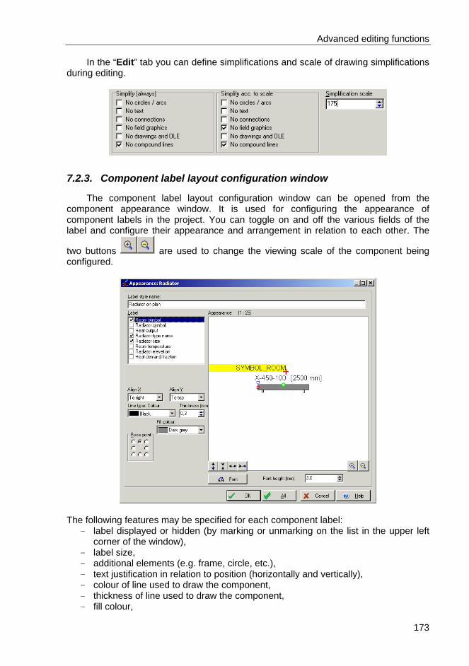
Advanced editing functions
173
In the “Edit” tab you can define simplifications and scale of drawing simplifications during editing.
7.2.3. Component label layout configuration window
The component label layout configuration window can be opened from the component appearance window. It is used for configuring the appearance of component labels in the project. You can toggle on and off the various fields of the label and configure their appearance and arrangement in relation to each other. The
two buttons are used to change the viewing scale of the component being configured.
The following features may be specified for each component label: - label displayed or hidden (by marking or unmarking on the list in the upper left
corner of the window), - label size, - additional elements (e.g. frame, circle, etc.), - text justification in relation to position (horizontally and vertically), - colour of line used to draw the component, - thickness of line used to draw the component, - fill colour,

Advanced editing functions
174
- text orientation, - base point, - component shape, - line linking the component with its label displayed or not,
- buttons in the lower left corner of the component display area “Increase / decrease component height / length” enable changing the dimensions of the component and checking the manner of mutual displacement of labels when the dimensions are changed.
Moreover, the following can be specified for the entire label:
- font type and size, - font heigh – nominal value for the reference scale.
♦ To change the font (simultaneously for all label fields), click on the “Font” button and
select a font. You can also specify font size in millimetres.
♦ To change the relative size of font for individual fields select a value in the “Size” field for each label.
The current field may be selected in the list displayed in the upper left corner of
the window. After selecting a field, a red cross and a green circle appear on the graphical
symbol of the component. The red cross indicates the point of “attaching” the field, and the green circle determines the so-called base point.
The base point is of significance in case of components of variable height. It indicates the point to which the caption is to be attached when the component size is changed. In effect the red cross indicates the position of the caption in relation to the base point. For instance, if the base point is in the middle of the upper side, the label field will always be positioned at the same distance from the middle of the upper side. If the red cross coincides with the green circle, the caption will always be positioned in the middle of the upper side.
! Not all fields described above are available for each component.
Confirm the settings in the component appearance window by clicking “OK” or
cancel them by clicking “Cancel”. For some labels an “All” button is available for simultaneous changing of appearance of all labels of a given type.
7.3. Graphical editor configuration
Application configuration is meant as settings, which are not saved in the project (and therefore do not depend on any particular project), but are saved to a configuration file and are assigned to a particular user. This is the main difference between project options and User settings and remaining application configuration.

Advanced editing functions
175
7.3.1. User settings
♦ To display user settings window select “Options / Settings”.
The “Program settings” window has four tabs: - “Designer data” – here you can append text data on the company, investor and
designer. - “Screen appearance” – here you can specify how part of the screen should look
and the colours used in editing. - “Files” – here you can specify what happens upon opening a file, automatic file
saving frequency and saving options on exiting the application. - “General” – here you can specify other settings. - “Messages” – here you can specify which warnings and hints are not to be
displayed upon completing calculations.
“Screen appearance” tab: - “Show” – toggles on and off rulers and status line. - “Status line” – status line options. - “Hint area shape” – enables specifying the shape of hint area which is displayed
when you position the mouse pointer on an item on the screen. - “Hints in data table” – when you position the mouse pointer on some of the fields
in the data table, hints are displayed. Here you can switch off the display of these hints.
- “Hints for project components” - when you position the mouse pointer on a project component, hints are displayed with that component’s data and, if available, calculation results. Here you can switch off the display of these hints.
- “Show group in data table as ...” – when a fitting component is placed on a component (e.g. a valve on a pipe-run), the data table includes both the pipe-run data and the valve data. The valve data may be displayed or hidden (see section 4.10.5). Here you can determine the manner of presenting data upon marking a component.
- “Auxiliary windows” – these include: data table, error list, data sets list, letter shortcut list, etc. Here you can force these windows to be displayed without titles. This enables more information to be displayed. Windows differ from one another in colour and contents, so mistakes are unlikely.
- “Show layers as” – here you can determine how the project layers are to be displayed – as tabs or as check lists (see section 4.2).
- “Selected component colour” – colour in which the marked components are drawn.
- “Workspace colour” – background colour during editing. - “Crosshairs cursor” and “ Crosshairs cursor colour” – crosshairs cursor consists
of two perpendicular lines which are displayed in the workspace at the current position of the mouse pointer. This cursor facilitates positioning of components in relation to each other. Here you can switch this cursor on and specify its colour.
- “Zoom in/out increment” – here you can specify the percentage increment of zooming in and out (when using Zoom in and Zoom out commands).
- “Animate zoom in/out” – when this box is checked, the magnified/shrunk area is displayed by means of animated rectangles during zoom in/out. This helps to see how the viewed area is changed.

Advanced editing functions
176
“Files” tab: - “Position on open file” – project view displayed upon opening it. - “Lock on open file” – LOCK mode (section 4.6.2), which locks components. This
can be altered after opening the file:
1. “No change” – opening of a file does not change the current LOCK mode setting. 1. “Same as last edit” – the same LOCK mode is set as during last save of the file. 2. “Lock” – the LOCK mode is always enabled after opening of a file.
- “Error list on open file” – here you can specify whether the error list is shown
upon opening a file if errors occur. - “Autosave” – data can be saved automatically at specified time intervals. Here
you can toggle autosave on and off and specify the time interval. - “Read AUTOREAD for new data” – toggles on and off the loading of options and
initial project contents from the AUTOREAD file. You’ll find more information in section 7.16.
- “Display welcome window on start-up” – here you can specify whether the welcome window (with three basic commands: New, Open, Open last) is to be displayed on program start.
- “Save options” – here you can specify which settings are saved on exiting the application, this applies to: contents of toolbar, all settings in the “Program settings” window and screen layout (positions of such items as data table, error list, toolbars).
- “Save toolbar now” – enables immediate saving of the toolbar in its current state. - “Store names of last ‘x’ files” – the graphical editor stores the names of the files
recently opened and displays them in the “File” menu to facilitate their reopening. Here you can specify how many names you want to store.
- “Show recent file names with full path” - when this box is checked, the file names shown in the “File” menu are displayed with their full access paths. This is useful when you work with files saved to different disks.
“General” tab:
- “Message duration” – time duration of the display of minor messages in the status line (e.g. “cannot place component here”).
- “Undo options” – options of the Undo and Redo commands. You’ll find more information in section 4.7.
- “Restore screen position on Undo and Redo” - when this box is checked, the program tries to restore screen position and zoom level on "Undo" and "Redo". If the box is not checked, screen position is not restored.
- “Double click in data table” – operation executed when you double click on a selection field in the data table.
- “Select values in check lists by” – select single or double click for confirming selections in lists for selection fields.
- “Open group in check list by” – select single or double click for opening subgroups in lists for selection fields.
- “Immediately scroll with the slider” – When this box is checked, the view of the project on the screen is moved as you move the slider on the horizontal or vertical scroll bar. When this box is not checked, the view of the project on the screen is refreshed only after you stop moving the slider.
- “Display calculation results after changing project” – when this box is checked, calculation results are still displayed on the drawing even if data have been

Advanced editing functions
177
changed. Only the status icon changes to indicate that the project has been changed. When this box is not checked, calculation results disappear after each data change.
- Print options: • “Print on margins” – when this box is checked, the margins are available for printing.
When this box is not checked, one letter in the text may be lost in the printout when page break is inserted in the middle of text.
• "“Print page header vertically” – when this box is checked, page header (information on project name and page number) will be printed vertically on the left side of page instead of being printed horizontally in the upper left corner of page.
• “Print page header on page 1 only” - when this box is checked, page header (information on project name and page number) will be printed on first page only.
• “Print scissors – paper cutting lines” - when this box is checked, small scissors symbols will be printed to indicate location of page cutting.
• “Print paper cutting lines” - when this box is checked, broken lines will be printed to indicate page cutting lines.
• “Print numbers of adjacent pages” - when this box is checked, arrows and numbers of adjacent pages are printed on margin.
• “Warn when trying to print without calculations” - when this box is checked, a warning will be displayed if you try to print a project which has not been calculated or which has been altered since last calculations have been done.
A button in the lower part of the window enables configuration of colour
conversion table for exporting DWG/DXF files (to AutoCAD®). Each colour displayed by the graphical editor can have a number assigned, corresponding to the colour used in AutoCAD®. In addition, you can toggle on and off the use of Windows fonts in DWG/DXF files.
“Messages” tab:
- Here you can specify which of the warnings or hints are not to be displayed upon completing calculations. Message disabling applies to the entire editor, but it can be set at any time.
- A message can be disabled in the program settings or directly by pressing the right mouse button when the mouse pointer is over the message in the error list. Then select “Don’t show this message again”. The selected hint or warning will not be displayed the next time you start calculations.
7.3.2. Screen appearance configuration
Basic screen components are described in section 4.2. Apart from the main window there are auxiliary windows, which may be pasted into the main window and function as its part or as separate windows displayed over the main window.
Each auxiliary window that can be pasted into the main window (except for toolbars) has a set of special buttons in its upper right corner:

Advanced editing functions
178
is used for closing the auxiliary window. is used for moving the window on the screen. When moving the window its
frame may be wide or narrow. The width of the frame depends on the location of the window. Wide frame indicates that the window will be independent, narrow frame indicates that the window will be pasted into the main window area. Narrow frame appears only when the auxiliary window is moved to the edge of the main window where it can be pasted.
When you position the mouse pointer on the button, a hint appears with information on the auxiliary window, and when you press the mouse button the entire help page is displayed.
Pasting toolbars into the main window is done the same way as pasting auxiliary
windows. The only difference is that there are no special buttons on the toolbars. However, when you position the mouse pointer next to a button or between buttons of the toolbar, the pointer takes on the shape of a grabber hand which enables dragging the toolbar into another location on the screen.
The main (standard) toolbar is displayed in the graphical editor screen upon launching the program. It contains tabs, which enable switching between parts of the toolbar.
Apart from the main toolbar, you can also place other toolbars on the screen. These toolbars are copies of the main toolbar tabs.
♦ To place additional toolbars on the screen:
1. Press Shift+F9 or click the right mouse button on the main toolbar within an area with no button.
2. Mark the toolbars which you want to place separately on the screen. 3. Click on the “Close” button. 4. Move the new toolbars into appropriate location.
You can move the main toolbar around the screen just as any other toolbar. If,
however, the main toolbar is pasted at the side of the main window, the tab names are not displayed. Instead of tab names, an empty field is displayed. Pressing the right mouse button when the pointer is within that area displays a menu that enables selection of any of the tabs.
Other screen appearance settings are defined in the program settings window on the “Screen appearance” tab (see section 7.3.1).
7.3.3. Configuring toolbars, keyboard, mouse and pop-up menu
The graphic editor enables you to configure the contents of toolbars, assign operations to individual keys and keyboard shortcuts, configure operations executed on pressing mouse buttons and define the contents of pop-up menu. You can execute these operations in the “Configure” window.
♦ To display the window for configuring toolbars, keyboard, mouse and pop-up menu select Options / Configure ...”.

Advanced editing functions
179
The window has three tabs. One of them is used for configuring toolbars, the second is for configuring the keyboard and the mouse, the third is for configuring the pop-up menu.
Toolbar configuration:
In this part of the window (i.e. the first tab) you can specify the contents of all
toolbar tabs. A list of operation categories is displayed in the upper left part of the window.
When you select one of the items in the list, available operations in the form of buttons are displayed in the upper right part of the window or a list of modules appears. When you position the mouse pointer on a button, its function is displayed.
The lower left part of the window contains a list of available toolbars (tabs of the
main toolbar) and buttons for creating a new tab, deleting and renaming an existing tab. Two buttons with blue arrows to the right of the toolbar list are used for changing the sequence of tabs displayed within the main toolbar.
The central right part of the window contains the set of buttons of the selected toolbar.
♦ You can move the buttons from the upper part of the window to the lower part and
back by dragging and dropping: 1. Position the mouse pointer on a button and click and hold the left mouse button. 2. While keeping the left mouse button depressed, move the pointer with the button
to the desired part of the window. 3. Release the left mouse button.
You can delete buttons in a similar way by dragging them to the waste bin (also
displayed in the window).

Advanced editing functions
180
In the lower part of the window you can also change the appearance of buttons (“flat” or framed) and specify whether the hints for buttons are to display keyboard shortcuts.
♦ To create spacing between two neighbouring buttons, insert a “separator” between
the buttons. The separator button is the first button in the upper part of the window.
Buttons that represent modules may be configured.
♦ To configure a button that represents a module: 1. Click the button, then click “Configure”. 2. A window described in section 7.11.4 is displayed.
Keyboard and mouse configuration:

Advanced editing functions
181
On this tabs you can assign operations to individual keys of the keyboard or to key
combinations and assign operations to mouse buttons. A list of operation categories is displayed in the upper left part of the window.
When you select one of the items in the list, available operations of that category are displayed in the upper right part of the window.
♦ To assign an operation to a key or a combination of keys:
1. Select a category of operations. 2. Select an operation from the list of operations – the key combination to which
the operation is currently assigned is displayed in the “Current shortcut key” field. This field is empty if no keys are assigned to the operation.
3. Click on the “Press new shortcut key” field. 4. Press the key combination you want the operation to be assigned to. The
combination is displayed and a warning is issued if that combination has already been assigned to an operation.
5. Click on the “Assign” button. The selected key or key combination is assigned to the indicated operation.
6. The “Default” button restores the default keyboard configuration.
♦ To assign an operation to a mouse button: 1. Select a category of operations. 2. Select an operation from the list of operations. 3. Click on the appropriate “Button” and “Click” fields on the right side of the
window. Information is displayed on the operation currently assigned to the mouse button.
4. Click on the assigning button. 5. By pressing the “Cancel” button you can cancel the assignment.
Fields for configuring mouse wheels are in the right part of the window. For a
single wheel mouse, settings are those for a vertical wheel. For a dual wheel mouse,

Advanced editing functions
182
vertical and horizontal wheels may be configured separately. The use of mouse rolls and associated keys of the keyboard is described in section 4.3.
Pop-up menu configuration:
In this part of the window you can define the contents of pop-up menu, the
invoking of which may be assigned, for instance, to the right mouse button. A list of operation categories is displayed in the upper left part of the window.
When you select one of the items in the list, available operations of that category are displayed in the lower left part of the window along with “(menu component)” and “(separator)” items, which enable inclusion of an operation that depends on the clicked component and of a separator – a line for separating menu lines, respectively.
A list of operations included in the pop-up menu is displayed on the right side of the window. You can change the sequence of functions by means of buttons with blue arrows on the right side of the list.
You can move operations from one list to the other by dragging and dropping or by using the “Add” and “Cancel” buttons.
The “Default” button restores the default pop-up menu.
7.3.4. Changing the sequence of data displayed in data table
Each time you select a component, its data are displayed in the data table. Sometimes not all of that data are necessary, sometimes a different sequence of the data would be more convenient. For this reason you can change the sequence of items in the data table and hide selected fields of the data table.
♦ To change the sequence of component data displayed in data table:
1. Select “Component data / Change data sequence / <component_type>”. 2. A window is displayed for changing data sequence. Data fields are displayed in
the sequence in which they are arranged in the data table; a symbol beside the field name indicates whether the field is displayed or not.

Advanced editing functions
183
3. Using the two arrow buttons on the right side you can move the fields into a different position (up or down). You can also do this by clicking on the field and dragging it.
4. To disable the display of selected data in the data table, uncheck the box to the left of the data name.
7.4. Using drawings from other applications
7.4.1. Importing drawings; Drawings gallery
The graphical editor supports use of drawings from other applications. Such drawings are treated as “pure” graphics, which means that they cannot be part of the calculated system. Drawings are handled in the “Drawings gallery”. In this window you can load drawings, delete them, re-scale them, modify their descriptions, etc.
♦ To activate the drawings gallery (window for handling drawings), select “Modules /
Drawings gallery...”.
The drawings gallery window is shown below:
The upper part of the window includes a list of drawings in the project. Some
items in the list may be preceded by symbols “L” or “U”. They have the following meanings:
- “L” – the drawing is saved to user library; it is saved to project file only if it was used. Drawing without the “L” symbol is saved to project file only and is not available in other projects
- “U” – drawing used in the project.

Advanced editing functions
184
After clicking the drawing title in the drawings list, the drawing is displayed in the lower part of the window. To zoom in or out the drawing use buttons with magnifying
glass , use the scroll bars to move the drawing horizontally and vertically. Check the box under the drawings list to save the selected drawing to user
library. You can change the label of the selected drawing in the “Label” field. Buttons for loading the selected drawing from disk, saving the drawing to disk and
deleting the drawing from the list are in the upper right part of the window. Drawings may be saved in several file formats.
! It is not possible to delete a drawing that is used in the project.
Tabs for configuring drawing data are on the right side. The “Scaling” tab is used
for scaling the drawing. You can move the red points anywhere on the drawing. Move both points with the left mouse button depressed to characteristic locations within the
drawing and enter the distance between them in the field . The drawing is re-scaled after clicking the “Scale” button.
You can specify the dimensions of the drawing in “X size [m]” and “Y size [m]” fields. These dimensions should be specified in an absolute scale in metres. If the “Proportions” box is checked, altering one dimension of the drawing forces the other dimension to change accordingly.
On the “Connections” tab there is a field, after checking which two spots appear on the drawing. You can move these spots with the left mouse button.
This function may be used to create drawings of such components as boilers and
terminal unit of specified pressure drop. It is also possible to change the drawing type for components inserted in the “Developed view” sheet. After placing the component in the workspace, change designation to “Drawing” in the “Drawing type” field of the data table and select the file saved to gallery in the “Drawing” field.

Advanced editing functions
185
The additional field “Grid” indicates that connection points can only be moved
along grid lines. The last two fields in the right-hand side of the window have the following meaning:
- “Display scale” – scale in which the drawing is displayed, - “Show size” – a blue broken line indicates the drawing border.
! The program enables importing graphic files in the DWG, DXF, WMF, EMF, BMP,
JPG format and others. When a DWG/DXF file is selected for loading to the gallery, the import window is opened.
7.4.2. Saving a fragment of project as a drawing
The previous sections describe how to use drawings from other applications as graphic components in the program. The program, however, features some simple tools with which you can create your own drawings. There is also a function which enables to place such drawings in the Drawings gallery and then to use them elsewhere and in other projects.
♦ To save a drawing in the Drawings gallery:
1. Make the drawing. You can use all components, including those from the “Graphics” tab.
2. Mark the components. You can use all the techniques described in sections 4.8.2 to 4.8.6.
3. Select “Modules / Save selected as drawing”. 4. The marked components are saved as a drawing and placed in the Drawings
gallery. Configuration of drawings in the Drawings gallery is described in section 7.4.1.
! Drawings in the Drawings gallery bear no design data. Only the drawing is saved
and it will not be possible to modify it in the future.
♦ To save a fragment of the project in the form of a set of program objects, mark the
components to be saved and select “Append to toolbar” in the “Modules” main menu.

Advanced editing functions
186
7.4.3. Using drawings
You can insert drawings anywhere within the project without any link with other components of the project.
♦ To insert a drawing into the project:
1. Select “Drawing” in the toolbar of the “Graphics” tab . 2. Move to workspace and place the drawing in the project. 3. Open the list in the “Drawing” field in the data table and select the drawing or
click “add new ...” to open the drawings gallery. “Yes” in the “Maintain size” field of the data table means that the dimensions of
the drawing specified in the “Drawings gallery” are preserved. When “No” is entered in that field, you can resize the drawing.
The “Displayed” field enables modifying the display of the drawing. When “No” is specified, the drawing disappears from the drawing area and only the olive oil frame remains.
7.5. Importing DWG/DXF file as plan with interpretation
A building base plan (plans of floors of the building) is necessary for designing radiant heating systems, and it is used during heat loss calculations. The base plan can be drawn directly in the program with the use of available components, or it can be imported from a DWG/DXF file with walls, windows and doors interpreted. During import appropriate layers are marked, from which the complete structure of the floor is generated – walls, windows and doors are inserted into the worksheet in the form of objects (the same as those inserted during manual creation of the base plan) and room structures are generated on their basis.
The file is imported into the current worksheet. Select “Import building plan from
DWG/DXF file” in the “File” menu. A new window is opened, where the file on the disk can be selected (the contents of the file are displayed in the upper right corner). Click the “Open” button. When importing for the first time, you will be prompted to specify the font file used in the project (with .shx extension). You can indicate a file on the disk – it can be provided with the project or it can be saved in AutoCAD folders. If the file is not available, click the “Cancel” button.
The file import window opens. All drawing layers included in the loaded file are displayed on the left side. A preview of the imported file is displayed in the upper main window of the screen. Buttons for viewing and moving the drawing and for measuring the lengths of components in the plan are locayed in the upper left corner of the svreen – these functions are enabled only after selecting the drawing unit of measure.
The drawing unit of measure is selected from a drop-down list box under the buttons. The unit must be appropriate for the actual dimensions of the object. The dimensions of the drawing, its width and height in DWG/DXF file units and in metres, are displayed below.
! The selection of the drawing unit of measure, appropriate for the dimensions of
the actual object, is important with regard to the graphical editor, which always

Advanced editing functions
187
displays and reads dimensions in metres. Therefore the imported drawing should be properly rescaled.
When you press the right mouse button within the drawing preview area, a pop-up
menu is displayed, which – in addition to viewing the drawing – enables selecting display options, that is the background colour and toggling between Paper <-> Model.
♦ To move the drawing preview press and hold the left mouse button and move the drawing in the desired direction. During this operation the mouse pointer takes on the
following form: . To move to the next import window click the “Next” button in the upper part of the
screen. The next stage is the selection of layers with walls. By default no layer is selected. Marking a layer blue causes it to be displayed as a broken line. Only after putting a tick in the box, the layer is displayed permanently and components of that layer are selected for interpretation.
By default walls drawn with two lines are interpreted. If more lines are used for a
wall, these may be misinterpreted. In such case click the button, move to the drawing preview area and mark the “multi-line” wall. The preview of the marked area and result of interpretation is displayed in the lower part of the window. Several characteristic fragments of walls should be marked – this way drawing types are created for walls in the file.

Advanced editing functions
188
If a wall drawing type has been marked unnecessarily or improperly, it can be deleted. In such case mark that drawing type in the “Selected wall types” and click the
button. In the upper part of the window the wall thickness range must be specified
(minimum and maximum value). If the project includes ventilating or chimney ducts, the wall thickness must be approprietely increased so that these components are
interpreted properly. You can make use of the “Length measurement” function here.
To move to the next import window – the window and door interpretation window -
click the “Next” button. At this stage mark the layers with windows and doors, enter appropriate value in the “Window width range” field. You can make use of the length measurement feature and select the highest value among all window and door widths – this must be rememberd about particularly in the case of double doors.
In the “Window and door types” in the “library” mark all types of windows and doors that are identical in drawing terms with those present in the imported drawing. Remember about marking double doors, if the project includes this type of doors.
To better see the components in the drawing use the buttons for magnifying and moving the preview in the upper part of the window.
After checking the selection of interpreted windows click “Next” to move to the last
import window. Here you select the layers that are loaded as a drawing, meaning that they are not interpreted. By default all layers are marked. When you press the right mouse button in the list of layers the options “Select all”, “Deselect all” appear. If the file is loaded with interpretation there is no need to load all layers again as the drawing background. You can abandon loading any layers at this point by clicking “Deselect all”. Or you can select only those layers that are necessary to append the graphics of the background drawing (e.g. stairs, furniture, etc.).
After clicking the “Next” button, the drawing is interpreted (which may take some
time to complete) and loaded into the project. Percentage of the interpretation completed is displayed, and when this is complete, an appropriate message appears. Click “OK” and the file is loaded onto the “Structure” layer of the current worksheet. Walls and rooms defined thereby are displayed on the screen.
Quality of the interpretation depends in the first place on the quality of the
DWG/DXF file loaded and on the interpretation options set (particularly the available wall thicknesses and widths of windows). Best results are achieved when walls and windows/doors are included in separate layers.
If the interpretation is not completely proper, you can make manual adjustments, such as drawing a wall, inserting a window or a door, etc.
7.6. Importing DWG/DXF file as plan without interpretation
A file generated with a CAD application can be used as a base plan, which can be loaded from a DWG/DXF file without interpreting its components.
The imported building drawing or map may form a background on which the structure of the building, installation or network can be plotted.

Advanced editing functions
189
To move to the next import window click the “Next” button in the upper part of the
screen. The next stage is the selection of layers with walls. Do not mark any layer. To move to the next import window – the window and door interpretation window -
click the “Next” button. As the file is not interpreted structurally, Do not mark any layer to analyse windows and doors.
To move to the next import window click the “Next” button in the upper part of the
screen. The next stage is the selection of layers that are loaded as a drawing. By default all layers are marked. Unmark the layers that are not necessary and that would unnecessarily complcate the drawing (e.g. room labels, numbers, titel blocks, etc.).
When you press the right mouse button in the list of layers the options “Select all”, “Deselect all” appear. You can deselect all layers or select only those, which are required as the drawing background for the project.
To complete loading the drawing, click the “Next” button. The drawing is
automatically loaded onto the “Base” layer, where the “DWG/DXF base” is placed with all selected layers presented in the form of a uniform drawing (without highlighting any object).
Components loaded without interpreting retain their structure from the DWG/DXF
file. When you move to the “Base” layer and click within the area of imported base, an olive green frame appears and base data are displayed in the table.
You can change the manner of displaying the entire base drawing or individual
layers. You can decide in which layers the AUTO mode is to be activated (by default all layers). This in practice means that when the AUTO mode is activated and you draw rooms or manually insert heating zones, the corners of these components are snapped to the marked layers. Similar operations can be performed by clicking the right mouse button on the base components. Then the layers which include those components are located and the display of those layers can be disabled and AUTO mode settings can be changed.
7.7. Exporting a drawing
The program enables exporting a drawing in the form of a plan, developed view, profile, system or network diagram into a file on disk. Drawings can be exported in the DWG, DXF, DXB, Windows Metafile (WMF files), Enhanced Metafile (EMF files), JPEG and other formats. DWG / DXF files can be opened in many professional graphics software packages, such as AutoCAD®. WMF and EMF files can be read by most Windows applications. The effect, however, can be unsatisfactory. Some applications may require appropriate graphical filter (e.g. for MS Office®, you can specify the graphical filters when installing the package).

Advanced editing functions
190
♦ To export a drawing select “File / Export drawing ...”. The export window is opened,
where you specify the type of file into which the drawing is to be exported.
! Export is not possible without specifying file type.
After selecting file type click the “Next” button. Another window is opened, where
you select the worksheets to be exported and specify the type of export. By default all worksheets are selected for export. If you don’t want to export some
worksheets, uncheck the fields next to those worksheet names. Export with appending is performed only in the case of DWG / DXF / DXB files.
This is characterised by the generation of a copy of the previously imported .dwg file and appending it with layers created by and saving it with a new name. The base on which the project was created does not need to be exported, as the entire structure of the .dwg file remains intact – it only includes additional layers with inserted components.
When the .dwg file was imported and it is on the disk, its name is displayed in the “Appended file” field. After marking a worksheet (highlighted in dark blue), additional icons appear and the appended file and the destination file may be changed. You can change the appended file or find the appended file on the disk, if its location has been
changed, by clicking the button.
! When the imported file is not on the disk or when it cannot be localised, a symbol is displayed. In this case you can look for the file manually or perform an export without appending.
! If there is more than one imported.dwg file on one worksheet, none of them will be appended and no name will be displayed. You can append only one of these files.
You can change the name of the destination file and its location on the disk with
the button. By default the name consists of the project file name + name of the worksheet. The file is saved to the data folder.
To export a DWG / DXF / DXB file without appending click on the button. Both the layers generated by the program and the base layers are exported. However the objects of the base will only be graphical objects, such as a line or a polygon, and will have no properties.

Advanced editing functions
191
Exporting of files other than DWG/DXF is done without appending any files. The name of the destination file can be changed.
To move to the last export window click on the “Next” button. Depending on the
file type selected, appropriate options are displayed: file version, unit, exported lines and their thickness or DPI resolution.
To complete the export and save the files to the disk click on the button. An “Exporting project as drawing. Please wait ...” message is displayed. Export is completed when the message disappears.
7.8. Numbering of rooms
The program features a function for semi-automatic numbering of rooms. The manner of numbering may be specified prior to importing or drawing the plan view of a storey.
In the building structure window (Ctrl+F7) there is a field
, which when clicked, opens a new window where a room numbering pattern can be specified.

Advanced editing functions
192
The algorithm of assigning numbers to storeys, apartments and rooms is defined
by entering characters described in the legend below into the fields on the left-hand side of the window. You can use numbers, letters and other characters.
After defining the algorithm in the building structure, assign a starting number or letter for the storey numbers in the “Symbol” field. Click OK to save the numbering method.
After creating or importing plan view of building, select “Assign numbers to rooms”
( ) from the „Component data” menu. Move to the drawing sheet and click the labels of individual rooms – the rooms will have numbers assigned to them in the order chosen by the user and in accordance with the defined algorithm.
The default numbering method is as follows: <storey_number><room_number> In this case rooms located on one storey have the following numbers: 001, 002,
003... etc., rooms on the storey above have the following numbers: 101, 102, 103... etc.
7.9. Defining macrodefinitions
Macros (macrodefinitions) perform the same functions as the specification of components for the “Miscellaneous fittings” field. They, however, facilitate that operation, as they constitute predefined sets of often-used components. As the program automatically sizes couplings and pipe fittings on the basis of graphical information provided by the drawing, the use of macros is recommended in specific cases only (e.g. when there are sets of components that cannot be automatically identified in the drawing).
Macros are defined in a special window in a similar manner to the specification of
miscellaneous fittings (see section 4.9.4).

Advanced editing functions
193
To define a new macro or to edit an existing macro select the “Options / Macros” menu (Ctrl+M).
Upon opening the “Macros” field a list of available macros is displayed. After
selecting a macro in the list you can modify it by removing or inserting components by means of arrows.
The buttons in the upper part of the window enable editing macro name, deleting and creating new macros. After creating a new macro, a new window opens where you enter the name of the macro. Then you can assign to the macro a catalogue loaded into the project. A list of existing macros is displayed at the bottom of the window. Upon confirming and clicking OK the new macro becomes the currently edited macro.
! Valves must be displayed in the drawing and they cannot be inserted by means
of macros.
7.10. Duplicating fragments of the project
Fast creation of a project may be facilitated by efficient duplicating of existing fragments. There are four basic methods of duplicating fragments of the project:
- copying to the clipboard and pasting, - saving fragments of the system as modules to a toolbar (see section 7.11.2), - duplicating by means of expanding groups, - duplicating fragments of the project in specified direction.
7.10.1. Copying to the clipboard and pasting
This is the simplest method of duplicating fragments of the project. The fragment to be duplicated may have its data already completed. Preferably it should be correct in formal terms (e.g. with internal connections made), as this facilitates further graphical editing of data.

Advanced editing functions
194
♦ To duplicate a fragment using the clipboard: 1. Mark the components you want to duplicate. You can use all the techniques
described in sections 4.8.3 to 4.8.6.
2. Select ”Edit / Copy” (Ctrl+C, ). The components will be copied to the clipboard as a module.
3. Select “Edit / Paste” (Ctrl+V, ). 4. Position the module in the required location. 5. Press the left mouse button. The module is now inserted. 6. You can insert subsequent modules by selecting “Edit / Paste” again or by
selecting “Edit / Insert last item” (F3, ).
! When pasting, you can make use of the possibilities of the AUTO mode described in detail in section 4.6.4.
! Components copied to Windows clipboard can be pasted as drawings into other applications (e.g. MS Word®, Corel DRAW! ®, AutoCAD®).
7.10.2. Duplicating by means of expanding groups
Duplicating of installation fragments by means of expanding groups enables fast creation of typical fragments of an installation, such as risers. You must, however, remember that in the case of expanding predefined groups (supplied with the program), the fragments created by ezpanding will not have their data appended automatically, i.e. the data included in the basic module will not be duplicated when expanding the group. If the duplicated fragments are to have their data appended, you must either create your own expanding groups (see section 7.11.5) and append their data at the stage of creating these groups, or duplicate fragments using the clipboard.
There are two ways in which fragments of installation are stored on the toolbar: in
the form of modules, which cannot be expanded automatically, or in the form of expanding groups, to which you can add subsequent modules when expanding the group in a specified direction.
! Expanding a frame of a group is not always equivalent to automatic self-
duplication of that group. The direction in which the group may be expanded and self-duplicated at the same time is indicated by arrows on the edge of the group frame.
♦ To place a fragment of installation and duplicate it by means of expanding groups:
1. Pick from the toolbar the required fragment of installation which is an expanding group. Each expanding group has one defined direction in which subsequent modules are added onto the group. This direction is indicated by two light olive-green arrows. For a riser, for instance, fragment of installation is represented by:

Advanced editing functions
195
2. Place the expanding group in the project. 3. The frame surrounding the group has eight square marks (handles) provided for
changing its dimensions. If you click and drag the square mark positioned between the two arrows, you will automatically add subsequent modules. This is what you get after expanding a riser by dragging the upper square mark:
! The placing of subsequent riser modules depends on the existing arrangement of floors. It is therefore advisable to specify floor elevations before expanding an expanding group.
Expanding groups of apartment systems may have similar properties. They,
however, would have to be expandable sideways. There are no restrictions on placing one expanding group within another
expanding group. Risers with apartment systems may be structured this way. The external group is the riser group. When you expand this group upwards you get subsequent storeys. Each storey has its separate internal group – an apartment system group. Each of these groups can be expanded sideways. This way you get subsequent receptors in apartment systems, separate for each storey.
! If you invert an expanding group before it is expanded, subsequent added on
modules will also be inverted.

Advanced editing functions
196
Remember that expansion of a group is not just duplication of the last storey, it consists in inserting new modules.
In addition to the standard expanding groups included on toolbars displayed after installing the program, you can define your own groups and place them on a new toolbar designed for user-defined groups and modules only.
You can find information on creating expanding groups in section 7.11.5.
7.10.3. Duplicating drawing fragments in specified direction
This is a method of fast duplicating of a fragment of the project while retaining one of its co-ordinates, e.g. elevation (duplication with horizontal translation). In some cases automatic determination of the location of the duplicated module expected by the User is not possible. Then it is best to use the clipboard to duplicate.
♦ To duplicate a fragment of the project in specified direction:
1. Mark the fragments you want to duplicate. You can use all the techniques described in sections 4.8.3 to 4.8.6.
2. Press Ctrl+Alt+Shift+<cursor control key> or the respective button on the
toolbar: , , . 3. Now you will be prompted for the duplication distance. Enter the distance
between the existing fragment and the new duplicated fragment. 4. Upon entering the value and clicking ‘OK’ the module or the marked set of
components is duplicated in the specified direction.
7.11. Modules
7.11.1. Modules - introduction
Although you can always create an installation using single components, using typical modules can speed up work considerably when fragments of the project are repeatable.
7.11.2. Creating and storing modules
Module is an arrangement of several components stored on the toolbar. The creation of a module consists in inserting components into the project, appending their data (if necessary) and storing on the toolbar. You can use existing modules to create new ones.
♦ To create a module and store it on the toolbar:
1. Using single components or other modules, create the fragment of installation you want to store as a module.
2. Mark all the components that are to make up the module. The best way to do this is to mark components in a rectangle (see section 4.8.5).

Advanced editing functions
197
3. Select “Modules / Add to toolbar”. The marked components are stored as a module in the “User” tab. The module configuration window is displayed (see section 7.11.4).
7.11.3. Modules gallery
You can view and edit all created modules in the modules gallery.
♦ To invoke a modules gallery select “Modules / Modules gallery ...” A modules gallery window appears:
A list of modules, arranged according to categories, is displayed in the upper part
of the window. After selecting a module in the list, the drawing of that module is displayed in the lower part of the window. Two buttons to the right of the list are used to delete and to configure a module.
You can set the size of the list area and the module view area by shifting the border between the two areas with the mouse.
7.11.4. Configuring a module
After clicking on the “Configure” button in the modules gallery window (see section 7.11.3) or in the “Configure” window (see section 7.3.3), the module configuration window is opened.

Advanced editing functions
198
Here you can: 1. Enter the text of the hint displayed when the mouse pointer is positioned over
the button on the toolbar. 2. Specify the category of the selected module. 3. Move the handle of the module. This is the point, where the mouse pointer is
located when inserting the module. The handle is indicated by a cross in the configure window.
7.11.5. Creating expanding groups
An expanding group is created in a similar manner to creating a module – it is made up of single components. The difference is that in the last stage you have to group the components and determine how the group can be expanded. We will illustrate this on an example of cold and hot water riser system with circulation.
♦ To create an expanding group:
1. Create a module that will be added on when expanding a group and store it on the toolbar as described in section 7.11.2. This may be, for instance, one storey of a riser system:

Advanced editing functions
199
2. If the basic part of the group differs from the module to be added on (e.g. a valve on circulation pipe-run is on the first storey), the required components must be added to the module being edited, if the basic part of the group does not differ from the module to be added on, skip this point.
1. Mark all components using the method of marking groups of components. 2. Group the marked components (see section 7.13). 3. Select “Modules / Group expansion manner”. 4. Specify the direction of expansion and the expanding module. The expanding
module should be a module created beforehand and stored, although this may be another module.
5. Click “OK”. Arrows appear beside the marked group indicating the direction of automatic expansion
6. Specify expansion distance in the data table: distance at which the subsequent modules will be positioned (in the case of groups expanding horizontally) or difference between elevations (in the case of groups expanding vertically).
! For groups expanding vertically the expansion distance specified here will be
applied during expanding only if the group is not placed on any floor elevation label type component.
1. Select “Modules / Add to toolbar”. The group is stored as a module in the “User”
tab. 2. Using Modules gallery (see section 7.11.3) or button configuration in the
“Configure” window (see section 7.3.3) you can change the module icon and insert a comment that will appear as a hint.
7.12. Drawing piping system within heating zones
The graphical editor features a tool for automatic drawing of the piping system forming a heating circuit. Sometimes, however, there may be a need to draw the piping manually – when, for instance, automatic drawing does not provide expected results, or when we want the piping to be drawn only in part of a heating zone. In terms of their properties, the lines drawn, either automatically or manually, are equivalent to polylines (graphical component). Data fields and properties of polylines for drawing piping are described in section 6.2.8.
! Polylines should be entered into the drawing at the end of the process of editing
the project, when calculation results are complete. Otherwise any change in calculations may make the polylines on the drawing invalid and necessitate editing them.
7.12.1. Automatic drawing
To enable automatic drawing of the piping use the component. After
selecting and moving to the HZ area, a cross is displayed, which indicates the connection point of pipe feeds to the HZ. In case of a “Spiral pipe pattern” specified in
HZ data, you have to indicate the direction of pipe laying: an arrow is displayed, which indicates the direction and a preview of the piping is displayed.
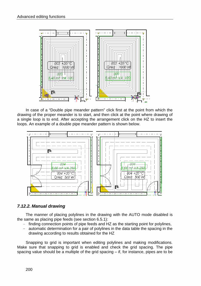
Advanced editing functions
200
In case of a “Double pipe meander pattern” click first at the point from which the
drawing of the proper meander is to start, and then click at the point where drawing of a single loop is to end. After accepting the arrangement click on the HZ to insert the loops. An example of a double pipe meander pattern is shown below.
7.12.2. Manual drawing
The manner of placing polylines in the drawing with the AUTO mode disabled is the same as placing pipe feeds (see section 6.5.1):
- finding connection points of pipe feeds and HZ as the starting point for polylines, - automatic determination for a pair of polylines in the data table the spacing in the
drawing according to results obtained for the HZ Snapping to grid is important when editing polylines and making modifications.
Make sure that snapping to grid is enabled and check the grid spacing. The pipe spacing value should be a multiple of the grid spacing – if, for instance, pipes are to be

Advanced editing functions
201
arranged every 12.5 cm, and the grid spacing is 5 cm, it will not be possible to draw polylines spaced apart at the required distance.
Disabling the ORTO mode is recommended when modifying segments of polylines already placed in the drawing.
! Although polylines representing piping look in the drawing like pipe feeds and
may form with them a whole on the printout, in calculations they are not treated as segments of heating pipes. In particular, they have no effect on heat and flow calculations and their connections are not checked.
This property of polylines makes them useful for drawing part of the heating
circuit, so that the fitter understands the intentions of the designer. Some examples of the use of polylines in manual drawing of piping system in HZ’s are presented below:
1. Meander pipe pattern – drawing indicates the point from which pipe laying
should start:
1. Spiral pipe pattern with occupied area. The polylines drawn indicate how irregularities should be taken into account – part of the room is covered by double meander pattern, which is shown in the drawing, the remaining part of the room, nearly square, is to be covered by a spiral pattern:

Advanced editing functions
202
1. Circuit with an integrated PZ at the beginning, drawn to such extent as to
indicate the type of peripheral zone (uPZ, not cPZ):
7.13. Grouping and ungrouping
Grouping of components is designed for creating a certain structure of an installation. For instance, groups are used for duplicating by means of expanding groups (see section 7.10.2), for renumbering of pipe-runs and appropriate presentation of calculation results.
Each group has the following characteristics:
1. None of its components may be placed outside the group. 2. When you move a group, all its components are moved with it. 3. When you move a group component outside of the borders of the group, the
extent of the group is automatically broadened.
♦ To group components: 1. Mark the components. You can use all techniques described in sections 4.8.2
and 4.8.6.
1. Select “Components / Group” (Ctrl+G, ).
! It is not possible to group one single component. A group is displayed surrounded by a brown frame:

Advanced editing functions
203
When you click within the group area where there is no component the group is
marked and group data are displayed in the data table. The marking of the group is indicated by an appropriate caption in the status line, by thicker lines of the group frame, and the contents of the data table.
! Make sure whether a group or only one of its components is marked – this is
particularly important when you intend to delete a group component only. You can create nested groups, which means that one group can be included
within another group. You can also ungroup components.
♦ To ungroup components: 1. Mark the group.
1. Select Components / Ungroup (Ctrl+H, ). 2. The group (as a kind of logical structure) is dissolved; but its components remain
in the drawing.
7.14. Finding a component
Finding components is a very useful function of program. A special window is designed for this operation:

Advanced editing functions
204
The upper field within this window specifies the type of component you are looking
for. In the field below you enter the symbol or the number of the component. After pressing Enter or clicking the “Next” button, the component is located and marked on the screen.
If a component cannot be found, appropriate message is displayed. You can display a list of project components of the specified type. To do this click
on the arrow button under the hand and question mark buttons. Clicking on an item in the list also starts a search.
7.15. Working on two or more projects simultaneously
Program Instal-therm is a single-document application, which means that at any given moment you can have only one document (project) opened. There is, however, no objection to running two or more instances of graphical editor at the same time. You can then open a different project in each instance of editor or you can open the same project in both instances, but activate other worksheet in each instance.
Running two instances of program facilitates the transfer of project fragments from
one instance to the other with the use of the Windows clipboard.
♦ To transfer project fragments into another project: 1. Start two instances of program. 2. In one instance open the project from which you want to transfer the fragment. 3. Mark the fragment to be transferred.
4. Copy the fragment to the clipboard: “Edit / Copy” (Ctrl+C, ). 5. Switch to the second program instance.
6. Paste the fragment from the clipboard: “Edit / Paste” (Ctrl+V, ).
7.16. AUTOREAD file
The AUTOREAD file is loaded as a base when creating a new project. In this file you can store default project options, print settings and possibly a fragment of project (e.g. a building plan, map, title block, etc.). When you install program there is available a standard AUTOREAD file.
♦ To create your own AUTOREAD file:
1. Create a project, which will form the base for other projects. This project can include any fragment of an installation. It can also be an empty project.
2. Specify project options. 3. Select “File / Save as ...”. 4. Type in AUTOREAD and press the Enter key.

Advanced editing functions
205
After carrying out these operations, the next time you create a new project, this AUTOREAD file will be used as a template. As normally such file already exists, you will be asked to confirm overwriting of the previous version.


Diagnostics and calculations
207
8. DIAGNOSTICS AND CALCULATIONS
8.1. Calculation method
8.1.1. Distribution of heat loss
The basis for sizing all terminal units in a room is the heat loss of that room (or ‘reduced’ heat loss, when radiant heating is also used in the room) plus part of heat loss of other rooms assigned to that room, and possibly minus part of heat loss assigned to other rooms. This value is called here the required output of terminal units – Qreq/Φreq.
The required output of terminal units is spread over radiant heating units,
convectors and other heaters, if any (e.g. electric heaters). The Qreq/Φreq distribution table is available both in Instal-heat&energy as well as in Instal-therm. If contributions of radiant and convection heating units are set to “auto”, then radiant heating prevails and it is designed in the first place. The remaining part of heat loss must be covered by the output of convectors. The calculated value is reduced by subtracting the estimated heat output of radiator circuit pipes and of other piping crossing the room (except for pipe feeds of radiant heating units, the output of which is already accounted for) and the result is the required output of convectors.

Diagnostics and calculations
208
8.1.2. Floor heating calculations
The applied methodology of design and calculations of heating output of hydronic floor heating systems is consistent with that described in the EN 1264 standard. Issues that have not been dealt with in the standard mentioned, were solved on the basis of documents supplied by manufacturers of floor heating systems and other available source materials.
The program follows a number of optimising procedures and applies a number of calculation algorithms. A short description of the most important of them is presented below.
Distribution of heat loss among HZ’s in the room If the user does not specify the contribution of individual HZ’s in the covering of
heat losses of the entire room, the distribution is done automatically during calculations. The algorithm of distribution takes into account the heating capacities of individual HZ’s providing a high level of optimisation.
The distribution follows the following guidelines:
Components that are part of system
designed
Q (terminal units with user specified
pressure drop)
Q (convectors)
Q (radiant heating)
Contribution to other rooms
Q
Qred
Qreq
Contribution from other rooms
Subtract loss across heated partitions
Room
Components that are not part of system
designed

Diagnostics and calculations
209
1. As far as possible a uniform output per square metre for all HZ’s in the room should be ensured to maintain the same average temperature of floor surface and provide favourable conditions of use.
2. In the peripheral zones output per square metre is increased in relation to occupied zones.
3. Check must be made to see whether each HZ is able to deliver the output assigned to it. If not, the distribution must be changed to match the values of assigned output to the heating capacities of individual HZ’s.
If it is not possible to distribute Qfh/Φfh in such way that all HZ’s are matched to
the assigned values, then the heat loss is distributed in such way that the deficiency or excess of output acquired from individual HZ’s in relation to Qfh/Φfh assigned to them is uniform – all HZ’s will have, for instance, excess output. When some HZ’s in one room have excess output, while the output of other HZ’s in the same room is too low in relation to assigned output, the distribution of output is not optimised.
Determination of the available pipe spacing options for each HZ The available pipe spacing options are determined for each HZ according to the
following guidelines:
1. Permissible pipe spacing in OZ and PZ is specified in general data. These depend on the applied fastening system and the type and diameter of pipe.
2. Non-standard pipe spacing settings in HZ data (if specified). 3. For HZ’s with an integrated PZ all combinations of permissible spacing values
for PZ and OZ are taken into consideration, provided that spacing in PZ is smaller than in OZ.
Calculation, for each pipe spacing, of temperature difference that provides the
required heat output. With the heating slab structure and floor covering and required heat flux density
(output per square metre) known, the program calculates the mean temperature of the heating medium in the circuit that would provide the desired output. Then, with the supply temperature known, the program calculates the temperature drop (cooling down of the medium) in the circuit required to provide the mean temperature of the medium.
The following limiting factors are taken into account when determining the temperature drop that provides the required floor heating output at the specified pipe spacing:
1. Maximum and minimum temperature drops for OZ and PZ specified in the
control circuit general data and, if necessary, amended in the HZ data. 2. For HZ’s that consist of a combination of uPZ/OZ (peripheral zone forming the
beginning of the entire circuit) the ∆t/∆θ_max is equal to ∆t/∆θ_max_OZ + ∆t/∆θ_max_PZ. The value of ∆t/∆θ_min is determined in a similar way.
3. The maximum point temperature of the floor surface (tfs/θfs max) determined in accordance with the EN standard cannot be exceeded. The method of determining tfs/θfs max defined in the standard takes into account the difference in floor surface temperature above the pipe and in the middle of pipe spacing – the floor surface temperature curve resembles a sinusoid. The larger the pipe spacing and the lower the thermal resistance of the floor covering – the lesser is

Diagnostics and calculations
210
heat dissipation and the larger are differences in tfs/θfs. Under these conditions the mean tfs/θfs is much lower than tfs/θfs max, as the peak of the sine curve cannot exceed tfs/θfs max.
4. The return temperature must be higher than ti/θi of the room. If the temperature difference that enables achieving the required mean
temperature of the medium is not allowed for any of the reasons listed above, the best available ∆t/∆θ for the given pipe spacing will be selected. This will result in excess / deficiency of output from the HZ in relation to assigned Qfh/Φfh.
If the limitations described above cause that for the given pipe spacing the interval of permissible temperature differences is empty, that spacing is not available. This situation may be caused by non-compliance with the standard with regard to tfs/θfs_max or by return temperature being too low in relation to ti/θi. If this applies to all available pipe spacing options, the floor heating in the HZ will not be sized and the entire block of results for this HZ will be highlighted in yellow.
Determination of pipe feed spacing and calculation of pipe feed output For each HZ with pipe feeds running across it, the area occupied by pipe feeds
and their output are calculated. The area occupied by the pipe feeds depends on the pipe spacing adopted. If automatic determination of pipe spacing is enabled, the spacing is determined according to the following rules:
1. For non-insulated pipe feeds, the pipe spacing is equal to that of the main circuit
in the HZ. This means that pipe feeds will occupy different areas depending on the current pipe spacing in the circuit. This solution may be treated as a simulation of the main circuit by pipe feeds, so that the floor temperature in the area where pipe feeds run does not differ much from tfs/θfs in the area of the main circuit.
2. For insulated pipe feeds the minimum pipe spacing is adopted. These pipe feeds are in practice excluded from heating and the area occupied by them is minimised.
! These fragments of pipe feeds are treated as insulated, which have the “I”
(insulated) option specified in the pipe feed data table. Pipe feeds with the “P” (in conduit) option are not treated as insulated. According to available manufacturers’ data, putting a pipe feeds into a conduit (casing) does not change significantly its heat output (low insulating power is compensated by increased heat exchange area).
To calculate the output of pipe feeds, their pipe spacing and average operating
parameters (mean temperature of heating medium) of the control circuit to which the pipe feeds are assigned are taken into account.
Selection of pipe spacing optimised with regard to heat output and flow

Diagnostics and calculations
211
The execution of the steps described above results in a list of available pipe spacing options and in the temperature drop and other heat calculation results for each of these spacing options. The pipe spacing selected is the best in terms of heat output and is hydraulically matched. The selection is based on the following criteria:
1. That spacing is selected, which ensures the attaining of the required output
(excess Qfh/Φfh is equal to zero or the value set in advanced options of calculations). During optimisation the program tries to select a pipe spacing with an output within “Matching” range. If there is no such spacing, that spacing is selected, which ensures an output within “Moderately unmatched” range.
2. If there are several spacing options that meet the above criterion, that spacing is
selected, which ensures the widest possibilities for changing the floor covering, meaning that adaptation to a floor covering with a different thermal resistance may be done by adjusting the flow rate.
3. Those spacing options that lead to non-compliance with the standard with regard to tfs/θfs max or to a return temperature being too low in relation to ti/θi, will not be listed and will not be made available to the user.
The structure of the system is optimised in terms of flow conditions. This means
that hydraulic parameters of pipe spacing options are taken into account when optimum options are selected (optimisation is done with regard to heat output – see above). The hydraulic parameters obtained are provided as results, and if the selected pipe spacing is correct in terms of heat output, but not correct with regard to flow conditions, then one of the many available methods of correcting hydraulic results must be applied (see section 9.8).
Determination of optimum supply temperature for each control circuit The optimisation algorithm uses defined temperature ranges fit for each room.
The temperature is assumed fit for the room when it is possible to attain the required output of floor heating in that room (total output of all HZ’s in the room). Depending on current data (type and number of HZ’s, required output of floor heating, permissible pipe spacing, temperature drops, etc.) the range of fitting temperatures may vary. In

Diagnostics and calculations
212
specific case there may be no fitting temperature, which indicates that it will not be possible to attain the required output of floor heating with the existing set of data.
For each temperature within the range between tsmin/θs min and tsmax/θs max
the pipe spacing optimised in heat output and flow terms for the HZ is sized, the quality of the solution is computed, temperature quality graph is plotted and temperature is selected from the highest quality range.
“Minimise ts/θs” optimisation After heat and flow optimisation the graph is corrected. In this case the lower the
supply temperature the better: the graph is modified, and if there are several high quality ranges, then the lowest temperature that meets the quality requirements is selected.
“Minimise cost” optimisation After heat and flow optimisation the graph is corrected. In this case the total length
of pipes and the number and sizes of manifolds are taken into account. The temperature selected should ensure the lowest possible number of manifolds with the lowest possible number of ports and the shortest possible length of piping. The heat and flow graph is modified using the calculated cost and the corrected graph is used to select the supply temperature.
8.1.3. Heater sizing
Sizing of convectors is performed according to the following principles:
- the heat output of convector should be as close to the required as possible; undersizing and oversizing of convector is acceptable,
- dimensions of the convector should fall within set limits (length, height and depth separately). These limits are also imposed by the lengths and heights of recesses under windows taken from the base drawing: plan view and data on building structure. An alternative is the “Smallest within range” method, where

Diagnostics and calculations
213
minimum and maximum dimension must be specified. You can combine the two methods, e.g. apply “Fit to recess” method for the height, and “Smallest within range” method for length and depth. In this case the smaller depth is preferred,
- to the required output allowances are added for enclosure, location (not under window) and non-standard manner and direction of supply. If an integrated convector or a convector with thermostat on circuit pipe is used, an allowance for faster heating of room after heating output drop is also taken into account.
The heater is selected from a catalogue and from selected folder with, for
instance, a range of heaters of similar design and various sizes. Particular sizes may have various availability status assigned – available immediately or on request. In calculation options you decide individually for every catalogue used whether this status is to taken into account.
The heat output of each sized heater is converted into thermal parameters (supply
and return temperature, room temperature) using formulas specified in the EN-442-2 standard. This ensures that calculations are accurate within a wide range of parameters of the medium, including temperature drop. Initial return temperature is assumed on the basis of data, as every heater has a specific Delta_t indicating expected temperature drop of the medium. After final sizing this value usually differs from the initially assumed. This is because the temperature drop is adjusted in such manner as to provide the required output from the heater (usually oversized, rarely undersized). The same adjustment is made for heaters of user-specified size. Adjustment limit is specified in calculation options.
8.1.4. Flow calculations and system adjustment
After sizing diameters of pipes and determining pressure drops on all pipe couplings and fittings and all terminal units, the required available pressure at sources is determined along with, when necessary, pumps on pipe-runs. At this stage radiant heating units and single-pipe systems are treated as internally adjusted and equivalent to terminal units of known pressure drop. Regulating fittings have initial pressure drop assigned equal to the higher of the two values: minimum internal pressure drop (DPmin) taken from data or pressure drop at maximum Kv.
The required available pressures are sized and calculated along with differential pressure valves. These components may often have the minimum stabilised pressure drop higher than that required by the stabilised circuit. This imposes higher requirements on the available pressure drop upstream of them. This does not apply to pressure relief valves, which are not strictly true regulating components.
If there is a bypass bottle in the system, it is treated as a no-pressure drop component (pressure difference between supply and return ports is equal to zero).
When pressure drop is determined (or specified) for the sources and pumps, system adjustment is performed: pressure drops in individual circuits are balanced in relation to each other and in accordance with the available pressure difference. If there are several control valves at different points between terminal unit and source, and the remaining excess pressure exceeds the required minimum pressure drops of these valves, their “weight” (participation in throttling of excess pressure) may be adjusted by means of a slider displayed on the flow calculation options screen.

Diagnostics and calculations
214
8.2. Invoking data diagnostic and calculations
After completing editing diagram of installation and appending data, you can proceed to calculations.
♦ To invoke calculations click on the button on the “Program” toolbar or select “File / Calculations...” (F10).
Data diagnostics are run and if there are no errors in data, proper calculations can
be initiated by clicking the “Next” button (you can also use Ctrl+Enter keys). A set of tabs is displayed for specifying calculation options. The last tab “Results” contains tables of calculation results. Actually the calculations are finally done when this tab is activated.
To disable calculations after displaying list of diagnostic messages, click the “Back” button or press the Esc key.
8.3. Data diagnostics
8.3.1. Types and syntax of messages
There are several windows and lists that display messages regarding the various stages of editing and calculating the heating system. All of them are uniform with respect to syntax and the manner of finding components to which these messages pertain.
The syntax of the message is as follows: [Message_type] Component_to_which_message_refers Message_text There are following types of messages:
Errors These are the most important messages, they are displayed in capital letters. All errors that occur in the course of creating a project must be rectified; otherwise it will not be possible to obtain all results for the project.
Warnings These messages are of lesser importance than errors. They are displayed in small letters and they do not block further calculations or display of results. Warnings are usually associated with data or results that are presumably incorrect and should be checked.
Hints The purpose of these messages is only to remind you of or draw your attention to some data or results. Like warnings, hints do not block further calculations or display of results and are also displayed in small letters.

Diagnostics and calculations
215
Connections These messages are warnings, which may appear after calculations are finished. They apply to automatic sizing of connections in the system and describe cases, where no connection or junction has been sized.
You can display information on the errors in the windows that show messages. To
do this click on the error and press the F1 key, or press the right mouse button and from the pop-up menu select “More info on message”.
A more detailed description of diagnostic messages is given in an appendix at the
back of this manual.
8.3.2. Checking connections
Before invoking calculations and the thorough data diagnostics associated with that, it is advisable to check the connections. This consists in making sure that there are no unconnected components. If there are connection errors in the system, they will be indicated in the diagnostics results window displayed after invoking calculations, so it is more convenient to make the necessary corrections before invoking calculations.
♦ To start connection checking select “Component data / Check connections”
(Shift+F2). A window is opened with a list of messages on connection errors found in the
system:
The structure of this window, types of messages that appear there and the
manner of finding components associated with the errors are identical to that of the diagnostics window and are described below. If the system is completely correct, the window is empty.
Data editing is not possible when the connection diagnostics window is displayed – you have to close it by clicking on the “OK” button. Information on erors is not lost – it will be displayed in the error list of the graphical editor.
8.3.3. Data diagnostics
Always after invoking calculations a data diagnostics run is made and the diagnostics results window is displayed. The diagnostics window does not appear if there are no messages to display – then the first calculations tab is automatically selected.

Diagnostics and calculations
216
The window displays messages on incorrect or suspected data found during the
diagnostic run. If connection errors are found, appropriate messages are displayed and other data are not checked. These errors must be corrected and calculations should be invoked again.
The types and syntax of messages and the manner of finding components
associated with these messages is described in the others subsections. After analysing the diagnostics messages you can go back to editing and
correcting data (press the “Back” button) or proceed to calculations (press the “Next” button). If errors occur, you cannot carry on with the calculations: an appropriate message is displayed in the lower left corner of the window and the “Next” button is not available.
If you go back to editing all messages that were displayed in the diagnostics
window are transferred to the error list (see section 9.7). You can then easily find and rectify all irregularities in the data.
8.3.4. Finding the component or field to which a message applies
When browsing the message list in the graphical editor the mouse pointer positioned on the message takes on the form of a “grabber hand”. When you click on the message, the component or field to which the message applies is marked and highlighted in yellow.
! Apart from being highlighted in yellow, the component to which the message
applies is marked (selected) and its data appear in the data table (if it is displayed).
This way you can easily find the cause of errors or data associated with the
warnings or hints. You can also obtain more information on the message. Mark the selected
message and press the F1 key or press the right mouse button to display the pop-up menu and select the appropriate item in the menu.
In the pop-up menu of the message list that appears after pressing the right
mouse button there is also a function for marking all components where the given error has occurred. This function facilitates correction of the same type of error, which may be rectified in a group of components simultaneously – data of all marked components is displayed in the data table where they can be modified at once (see section 4.9.7).

Diagnostics and calculations
217
An example of an error that can be corrected in this way is the “pipe type not specified” error.
The list of messages in a project which consists of many worksheets may have a
tree structure (when messages apply to several worksheets):
In the example above the list of messages for the “Worksheet 1” worksheet is
collapsed – this is indicated by the plus symbol in the square to the left of worksheet name. The “Worksheet 2” worksheet has a minus and messages for this worksheet are displayed.
♦ To expand / collapse the list of messages that apply to the given worksheet, click on
the square to the left of worksheet name or double click on the worksheet name in the error list.
When messages are marked, worksheets are automatically changed so that the
component to which the marked message applies is shown.
8.4. Calculation options
When you click on the “Next” button in the diagnostic messages window (which is possible only if no errors were found), the window is closed and a set of tabs with calculation options appears – values that have substantial effect on calculations and results, which in principle form an extension of the general data of the project, but for the user’s convenience have been moved out of the graphical editor to enable fast execution of several calculation variants. During the first attempt to run the calculations of a new project the values displayed in these fields are taken from the AUTOREAD file (unless the project is a modification of another project). During subsequent calculations these values are taken from the project file. Some options associated with pipe catalogues (e.g. maximum velocities) are taken for the first calculations from the pipe catalogue.
First the supply temperatures of individual control circuits of radiant heating
system have to be determined. Then floor heating calculations are performed. If no error messages appear, calculations may be continued by selecting the tab with diameter sizing, flow calculation, system adjustment and heater sizing options. After specifying these options, select the tab with calculation results.
If an error is detected in radiant heating calculations, these cannot be continued – the cause of the error must be eliminated.
If no radiant heating is provided in the project, the only displayed tab will be the one with diameter sizing options, flow calculations and system adjustment, heat calculations and result editing.
Calculations are completed when the “Results” tab is activated.

Diagnostics and calculations
218
Fast calculations It is possible to run the so-called “fast calculations”. In this case calculations are
performed without going through all the calculation options tabs (default values or values specified before are adopted).
! Running complete calculations with calculation options specified is
recommended in the first stage of the project. This function is useful when you want to refresh results displayed in the graphical
editor (without viewing results in tables), or when you make slight corrections in the project and want it to be recalculated. A message on the course of calculations is displayed and then the results in the graphical editor are refreshed.
All screens with calculation options are described in detail below.
8.4.1. Determining supply temperatures for control circuits
When calculations of a new file are done for the first time, the supply temperature of control circuits is determined automatically (depending on the specified or default temperature at source). When calculations are invoked the next time, ts/θs is equal to the one set before. A separate set of fields and buttons for specifying the supply temperature for each control circuit is displayed:
Control circuit: Name of control circuit, taken from temperature reducer or source supplying the circuit. “Opt. ts/θs” button Clicking this button invokes the optimising procedure described at the beginning of this section and substituting the circuit supply temperature with the calculated value. Supply temp.: This field displays current supply temperature, which will be used in calculations. You can enter the value directly from the keyboard or set it by means of up and down arrows. This enables specifying the temperature when it is determined by the parameters of the heat source (e.g. heat pump). The supply temperature can also be determined optimisation or from the ts/θs graph (see below). “Graph” button Displays graph of fitting ts/θs for individual rooms, described in detail in the following subsection.
“Use real temp. drop” button When this button is clicked, the calculated temperature drop between the mixer and source or temperature drop estimated according to the adopted indicator of temperature drop in pipe-runs (when calculations are done for the first time) is taken into account.

Diagnostics and calculations
219
There is an “Advanced” button in the upper part of screen above button and value
bars. Click this button to access supply temperature optimising parameters.
8.4.2. Graph of fitting ts/θs and optimisation of ts/θs on the basis of the graph
Available supply temperatures are marked as horizontal lines in the graph. The
range of scale depends on ts/θs min for the control circuit and ts/θs max of this circuit (defined in control circuit data in project options). Rooms assigned to this circuit (rooms with HZ’s connected to manifolds assigned to this circuit) are marked on the vertical axis.
The dashed vertical green line marked on the horizontal axis with a triangular slider indicates the current supply temperature setting. To change ts/θs you can use the numeric field beside the ‘Determine’ button or drag the slider or the line with the mouse pointer to the left or to the right.
The main feature of the graph are the intervals (ranges) of supply temperature determined by the program fitting the individual rooms. The fitting ts/θs is such temperature, that enables attaining from HZ’s within the room an output equal to heat demand to be covered by floor heating. These intervals are indicated by horizontal lines positioned at the level of the room name:
The green horizontal line in the drawing above indicates that the required floor
heating output will be attained in the “Room”, if the supply temperature is within the range of ca. 39.5ºC to 52.5ºC.

Diagnostics and calculations
220
The fitting ts/θs line is green, if it is intersected by the vertical dashed line
indicating current ts/θs setting. Blue colour indicates that ts/θs is too low, red colour – ts/θs too high. This may be interpreted as expected underheating or overheating of the room. In practice, however, it may occur that the room indicated by a red line (expected overheating) will show shortage of output, because the variants of small spacing in the pipe laying pattern may be rejected due to non-compliance with the standard with regard to floor surface temperature (tfs/θfs).
! The interval of fitting ts/θs displayed on the graph may in practice be discontinuous – the determined ts/θs is within the interval range, but the calculation results indicate shortage of or excess output. Such a situation is particularly probable, when a narrow range of permissible drop of medium temperature in the circuit is specified (e.g. ∆t/∆θ max. is 10 and ∆t/∆θ min is 6). However, in such cases the shortage or excess output is usually low.
It may occur, that the required output cannot be provided by floor heating (e.g.
when the required output from square metre is too high) and the ts/θs interval is empty – “No fitting ts/θs” message is displayed, accompanied by a red arrow pointing to the left or a blue arrow pointing to the right. The arrow type indicates the reason why there is no fitting ts/θs interval:
– indicates that all available ts/θs cause underheating of room. Most often the cause of that is that the heat demand per square metre of effective area of HZ is too high – due to the limitation of floor surface temperature, the maximum output from square metre of surface is ca. 100 W. Note that max. tfs/θfs is defined for a point, not as an average. Therefore the limit average output may differ significantly from the theoretical value of 100 W.
– indicates an opposite situation - all available ts/θs cause overheating of room (output obtained from HZ is higher than required – does not mean that maximum tfs/θfs is exceeded!). This often happens in case of rooms situated in the interior of a building, where heat losses are very low.
Buttons at the bottom of the graph window:
“Determine” Optimisation of supply temperature. Similar to the ‘Determine’ button on the control circuit bar – determines optimum supply temperature. “Adopt” Adopts temperature currently set on the graph, no matter whether it was determined by means of the “Determine” function or set manually. The graph window is then closed and the value specified on the graph will appear in the “Supply temp.” field of the control circuit bar. “Cancel” Cancels the changes made on the graph or in the numerical field and closes the graph window. The supply temperature remains the same as it was before opening the graph.

Diagnostics and calculations
221
The graph is an excellent source of information on the expected results of calculations. It helps determine, without studying numerical results, which rooms will be provided with the required heat output and which will not. You can then go back to editing right away and modify data, and then, after analysing the graph again, see whether the changes have produced desired effects.
Virtually all parameters of rooms and HZ’s in rooms accounted for in the
calculations have an effect on the range of fitting ts/θs, that is on the length and position on the graph of the line assigned to the room. The most important parameters are:
- required output in W/m2, which follows from the effective area of the HZ’s in the room and the value of Qfh/Φfh,
- type (thermal resistance) of floor covering, - range of permissible temperature differences (∆t/∆θ – temperature drop of
heating medium in the heating circuit), - available pipe spacing values, - presence and type of peripheral zones, - area occupied by pipe feeds and the manner of taking account of them.
The changes in these parameters have an effect on the changes of the fitting ts/θs
interval, and in consequence on calculation results obtained at given supply temperature.
Other use of the graph is the maximisation or minimisation of ts/θs. The graph
shows which rooms are “given up” (we allow their over- or underheating) by, for instance, reducing the supply temperature, or the opposite – how much can ts/θs be decreased without “giving up” any room.
For each temperature within the range between tsmin/θs min and tsmax/θs max
the system is optimised and temperature quality graph is plotted. A line indicating temperature quality is displayed in the temperature optimisation preview. To hide or display the quality graph check / uncheck the in the lower part of the window..
8.4.3. Radiant heating calculation options
The next tab displays – after determining the supply temperature and opening the tab or clicking the “Next” button – results of radiant heating calculations, which by now have been performed. This tab is described here, as it is possible on this tab to adjust manually the pipe spacing values for individual heating planes. At this stage already messages on errors in radiant heating calculations may occur and make further calculations of the entire system impossible. A yellow window with error messages appears then, and fields in the result table corresponding to these errors are highlighted in red. You can get more information on selected errors by clicking individual errors in the message window (cursor in the result table marks the appropriate fields) and then pressing the F1 key.

Diagnostics and calculations
222
The centre of this tab is occupied by the table of results. At the bottom there is a
table with yellow background for messages referring to calculations. Yellow colour also highlights these rows or cells of the table where warnings have occurred.
The structure of the table is as follows:
Manifold label
The line with manifold label (description) starts at the left edge of the calculation options tab. All lines located below, down to the next manifold label or label of HZ’s heated by pipe feeds, display results for rooms and their HZ’s associated with the given manifold. The line describing a manifold consists of the following fields: - Type of manifold inserted: < Manifold_Symbol > – symbol (name) of the
manifold; - Supplied from: <Symbol_CC> (ts/θs = ...0C) – symbol of supply source of control
circuit to which the manifold is assigned and (in brackets) supply temperature determined for that circuit (in effect, the supply temperature of the manifold);
- No. of outlets: <...> – number of outlets in the manifold, including spare outlets, if such were specified in data;
- Settings on: <s.r.> – location of manifold valves on the supply (s) and/or return (r) side;
- G: <... kg/h> – total mass flow in manifold; - Avail. press. <... Pa> – pressure available at the manifold.
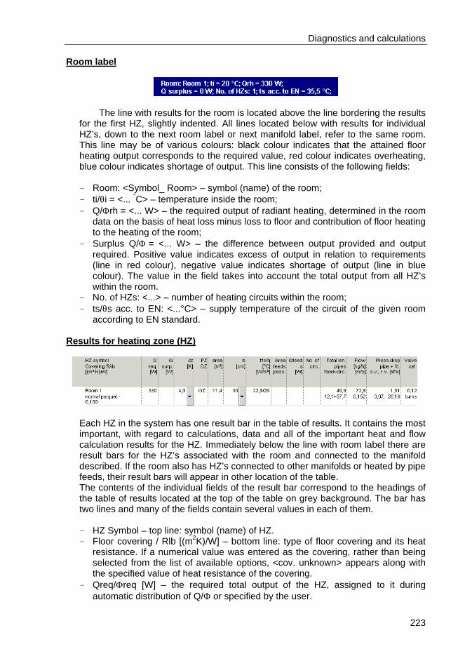
Diagnostics and calculations
223
Room label
The line with results for the room is located above the line bordering the results for the first HZ, slightly indented. All lines located below with results for individual HZ’s, down to the next room label or next manifold label, refer to the same room. This line may be of various colours: black colour indicates that the attained floor heating output corresponds to the required value, red colour indicates overheating, blue colour indicates shortage of output. This line consists of the following fields: - Room: <Symbol_ Room> – symbol (name) of the room; - ti/θi = <... °C> – temperature inside the room; - Q/Φrh = <... W> – the required output of radiant heating, determined in the room
data on the basis of heat loss minus loss to floor and contribution of floor heating to the heating of the room;
- Surplus Q/Φ = <... W> – the difference between output provided and output required. Positive value indicates excess of output in relation to requirements (line in red colour), negative value indicates shortage of output (line in blue colour). The value in the field takes into account the total output from all HZ’s within the room.
- No. of HZs: <...> – number of heating circuits within the room; - ts/θs acc. to EN: <...°C> – supply temperature of the circuit of the given room
according to EN standard.
Results for heating zone (HZ)
Each HZ in the system has one result bar in the table of results. It contains the most important, with regard to calculations, data and all of the important heat and flow calculation results for the HZ. Immediately below the line with room label there are result bars for the HZ’s associated with the room and connected to the manifold described. If the room also has HZ’s connected to other manifolds or heated by pipe feeds, their result bars will appear in other location of the table. The contents of the individual fields of the result bar correspond to the headings of the table of results located at the top of the table on grey background. The bar has two lines and many of the fields contain several values in each of them. - HZ Symbol – top line: symbol (name) of HZ. - Floor covering / Rlb [(m2K)/W] – bottom line: type of floor covering and its heat
resistance. If a numerical value was entered as the covering, rather than being selected from the list of available options, <cov. unknown> appears along with the specified value of heat resistance of the covering.
- Qreq/Φreq [W] – the required total output of the HZ, assigned to it during automatic distribution of Q/Φ or specified by the user.

Diagnostics and calculations
224
- Surp. Q/Φ [W] – the difference between output provided and output required. Positive value (red) indicates excess of output in relation to requirements; negative value (blue) indicates shortage of output. The sum of surplus outputs of HZ’s within the room is equal to the value in the “Surplus Q/Φ” field in the room label.
- ∆t/∆θ [K] – calculated temperature drop of the heating medium in the circuit. This always applies to the entire circuit. also in the case of an integrated peripheral zone (cPZ or uPZ).
The button on the right side of this field with an arrow pointing down opens a window for selecting automatic determination or manual specification of ∆t/∆θ. The appearance of the window is as follows:
- PZ / OZ – this field describes the contents of the following three fields with which it creates a set of results separated from other fields by continuous vertical lines.
If the HZ has no integrated peripheral zone, “OZ” appears in the top line in case of circuit that forms occupied zone or “PZ” in case of circuit defined as peripheral zone forming a separate circuit. Bottom line remains empty. In the case of HZ with PZ integrated with OZ, the top line displays “cPZ” for a PZ created by compacting the pipe laying pattern or “uPZ” for a PZ connected upstream of OZ. In the following three result fields, the first line refers then to this integrated PZ. The bottom line displays “OZ” and the second line of the following three result fields will then refer to the part of circuit that forms occupied zone. - area [m2] – effective area of HZ or of separate parts of HZ (see explanation of
“PZ / OZ" field). Covers the total effective area of HZ, including the area of pipe feeds running across the HZ. In case of HZ’s with integrated PZ, the area of pipe feeds is always subtracted from the part of HZ forming OZ, even if the pipe feeds on the drawing run across the peripheral zone.
- T (or other designation, depending on the manufacturer: B, b, p, r, VA; units: [cm] or [m] or [mm]) – pipe spacing within HZ or in its separate parts (see explanation of “PZ / OZ” field).
The button on the right side of this field with an arrow pointing down enables expanding a list of available pipe laying spacing distances for the HZ and selecting spacing other than default. The appearance of the list is as follows:

Diagnostics and calculations
225
The list includes a “Spacing ...” field, result fields for this option – “Surplus Q” and “td [K]”. If “Auto” is selected, the optimum option with regard to heating conditions is selected. If other option is selected, it will be labelled as “Manual”. The manually selected option is stored and will not be changed when doing subsequent calculations. To revert to optimum option select “Auto”. After selecting other pipe laying spacing option, it will be placed on the results bar of the HZ and the remaining result fields will be altered accordingly. If a pipe spacing distance causes excessive increase of tfs/θfs_max, even when using maximum temperature difference, a “Standard exceeded” message appears and this spacing becomes unavailable. If the return temperature is too low in relation to ti/θi, even at the lowest possible ∆t/∆θ, a “ts/θs too low” message appears and again the spacing becomes unavailable. When all options are unavailable, the entire result bar of the HZ is highlighted with yellow colour and appropriate message appears in the error list. - tfs/θfs/q [0C] / [W/m2] – temperature of floor surface (average) / heat flux density
(output obtained from 1 square metre) calculated for the HZ or its part (see explanation of “PZ / OZ" field).
- Area feeds pass. – surface area of pipe feeds running across. Displays the calculated total surface area of pipe feeds running across the HZ. The area depends on the lengths of individual fragments of pipe feeds and their spacing of pipe laying determined by the program or specified by the user.
- Qfeeds/Φfeeds [W] – output of pipe feeds running across. Depends on the total area of pipe feeds, spacing of pipe laying used for individual fragments of pipe feeds, insulation of pipe feeds, percentage of utilisation of their output and system operation conditions.
- Total len. pipes – top line: total length of pipes of the heating circuit, including the length of pipe feeds
- feed+circ. – bottom line: length of pipe feeds running from manifold to the circuit + length of pipe forming the proper heating circuit. The sum of these two values is equal to the total length in the top line.
- Flow [kg/h] – top line: mass rate of flow of heating medium in the circuit - [m/s] – bottom line: velocity of flow of heating medium in the circuit. - Press.drop pipe + fit. – top line: linear pressure drop in circuit including pressure
drop on pipe fittings connecting the manifold - s.v.; r.v. [kPa] – bottom line: pressure drop on valves installed on manifold. The
first figure represents pressure drop on valve on the supply end, the second figure is for pressure drop on valve on the return end.

Diagnostics and calculations
226
If the manifold is not adjusted, some of the fields may not be filled in. In the case of an adjusted manifold, this field will be displayed in bold font for the HZ that determines the required available pressure.
! Note: in order to calculate the total pressure drop after adjustment, the three values displayed in this field should be added together. The total should be approximately equal for all HZ’s connected to the manifold and should correspond to the pressure available on the manifold. If significant deviations of this total occur for some HZ’s, resulting from the valve adjustment range being exceeded, this will be indicated accordingly in the error list.
- Valve set. – setting of valve on the manifold. Letter in brackets indicates whether
the setting refers to the valve on the supply end – “(S)”, or on the return end – “(R)”. This field is filled in only when the entire manifold is adjusted.
The structure described above does not include zones heated by pipe feeds. As
these HZ’s cannot be assigned to any manifold (HZ may be crossed by pipe feeds running from different manifolds), results for HZ’s heated by pipe feeds are displayed separately and are grouped within a section following the last manifold of that sheet.
The relative arrangement of label of the group of HZ’s heated by pipe feeds, room labels and result bars for individual HZ’s is identical to that of standard HZ’s. The only difference is in the range of fields and their meaning.
Label of a group of HZ’s heated by pipe feeds
The status of the results header for this type of HZ is similar to that of the manifold label, it therefore borders with the left edge of the results tab. Room labels and result bars for HZ’s heated by pipe feeds of the sheet are displayed below. The header consists of the following fields:
Zones heated by pipe feeds assigned to source: <Source_Name> – name of the source supplying the control circuit.
Room bar
Results bar of HZ heated by pipe feeds
This bar has the same fields as that of a standard HZ. However, not all of them are filled in. Important fields include: - HZ Symbol – same as for standard HZ. - Floor covering / Rlb [(m2K)/W] – same as for standard HZ.

Diagnostics and calculations
227
- Qreq/Φreq [W] – same as for standard HZ. - Surp. Q/Φ [W] – same as for standard HZ. - area [m2] – same as for standard HZ. - T (or other designation, depending on the manufacturer: B, b, p, r, VA; units:
[cm] or [m] or [mm]) – pipe laying spacing valid for those pipe feeds running across the HZ heated by pipe feeds, for which the (auto) option was selected in properties. Some pipe feeds may be laid with other spacing specified by the user in properties. Detailed information is given in the table of results for individual pipe feeds displayed when printing.
- Area feeds pass. – same as for standard HZ. - Qfeeds/Φfeeds [W] – output of pipe feeds running across. It is also the total
output obtained from HZ’s of this type.
8.4.4. Other calculation options: diameter sizing
The following, third tab (first tab, when there is no radiant heating in the project) includes all the remaining calculation options: diameter sizing, system adjustment and heat calculations, including radiator sizing. To go to the required set of options select appropriate item in the list on the left side of the screen.
Diameter sizing options – the first set of options displayed – include the following
fields: - Resize diameters – enables diameter sizing during the second and subsequent
calculation runs of the project. - Retain user specified diameters – when diameters are sized, the values
specified in the editor are retained. - Skip to pipe successors – when there is no pipe of the selected type of
appropriately large diameter, another type – indicated as the “successor” - is selected from the catalogue (provided that it exists).

Diagnostics and calculations
228
- Skip to pipe fitting successors – some pipe fittings and couplings of narrower range of sizes may also have their “successors” with a wider range of sizes indicated in the catalogue.
The main components of the screen are two tables. The upper displays a list of
pipe types used in the project. The bottom table displays detailed options of diameter sizing for the type indicated in the upper table. These options include:
- Minimum diameter (inner) that can be used. - Multiplier for maximum velocity assigned to each diameter in the catalogue. - Maximum value of friction indicators.
Different values are specified for pipe-runs depending on their location: circuit
pipes, horizontal piping in apartments (connected to risers), risers and other parts of the system. Multipliers are used instead of specifying maximum velocity, as in some catalogues different maximum velocities are specified for different diameters. The multipliers used are saved to the project file.
A button ( ) in the selected line of the upper table opens an auxiliary table where
maximum velocities (with the multipliers applied) are displayed for the various diameters and where individual diameters may be toggled on/off to be or not to be taken into account when sizing.
8.4.5. System balancing options
System balancing options also include control of the sizing of the required available pressures for pumps and sources. The tab includes the following fields:
- Resize pumps on pipe-runs – enables pump sizing during current calculations; when a project is calculated for the first time this option is enabled automatically.
- Retain user specified Hpump on pipe-runs – when pumps are sized their delivery heads specified in the editor are retained; when this box is not checked, the delivery heads are deleted, as if “?” was entered as the delivery head in the editor.
- Allow larger diameter of DP valve – when this box is checked a pressure differential valve may be sized with larger diameter than the calculated diameter of pipe-run on which it is installed.

Diagnostics and calculations
229
A table specifying the following minimum pressure drops is displayed below: - on each terminal unit and its fittings, - on each control valve (except for those assigned to the first group – on terminal
units), - on each pressure differential valve.
These values may also be specified for each individual valve in the graphical
editor. Fields displayed below enable specifying the available pressure drop for each
source in the project or indicating that they should be determined automatically. You can also specify in advanced options for each source whether excess pressure is to be throttled by means of valves near the terminal units or near the source (if there are more control valves between source and terminal unit).
8.4.6. Thermal calculation options
The screen of thermal calculation options consists mainly of settings that control the sizing of radiators. It includes the following fields:
- Resize radiators (sizing is automatic when calculations are done for the first time),
- Retain user specified radiators (when sizing is enabled), - Adjust flow rates – adjust outputs of radiators, both sized and user specified, by
changing the flow rate of heating medium and return temperature.

Diagnostics and calculations
230
When radiators are sized or the outputs of user specified radiators are checked,
then the following values are taken into account:
- Radiator circuit pipe heat gain utilization [%] – value of less than 100 indicates that some of the heat dissipated by circuit pipes is not recovered in the room (is irreversibly lost).
- Riser heat gain utilization [%] – value of less than 100 indicates that some of the heat dissipated by risers is irreversibly lost.
- Warn, if gain contribution above.... – this value facilitates detection of cases, when a room is heated mainly by pipes running across it, which restricts the possibilities of adjusting heat output to the room. In this case a warning message is displayed during calculations.
- Do not adjust flow if oversized by... – radiator oversizing limit above which no further flow adjustment will be made (adjustment stops at this limit).
- Do not adjust flow if undersized by... – radiator oversizing limit below which no further flow adjustment will be made (adjustment stops at this limit).
A table listing the names of all radiator catalogues used in the project is displayed
below. You can make the following settings for each individual catalogue: - In stock only – select only these radiators, the availability of which is specified as
in stock; otherwise radiators are sized irrespective of their availability (information on availability is provided in the catalogue).
- Observe length restr. – indicates that restrictions on length specified in the data must be observed.
- Observe height restr. – indicates that restrictions on height specified in the data must be observed.
- Observe depth restr. – indicates that restrictions on depth specified in the data must be observed.
- Oversize for safety – oversizing of the radiator depending on local requirements (discrepancies between actual and design condition of building, use of thermostatic valves).

Diagnostics and calculations
231
! Note: radiator oversizing to account for enclosure type and connection type is done individually for each radiator on the basis of its data.
8.4.7. Result editing options
Result editing options have no effect on calculations and their results. They only specify the range of generated tables and lists and their editing. They have no effect on the graphical presentation of results.
The result editing options include the following fields:
- Generate bill of mat. – indicate whether the bill of materials is to be drawn up. Disabling this option may shorten the time taken by calculations of large systems on slower computers, when various variants are calculated and the bill of materials will be generated after accepting other results.
- Show integrated valves – indicate whether a list of integrated valves is to be drawn up. May be useful when integrated radiators are used with integrated valves ordered separately.
- Show existing components: With planned, Separately, Disregard – indicate whether components of the “Existing” status (set in data table of the component) are to be displayed in separate list tables, displayed together with components of the “Under design” status or not displayed in lists at all.
- Create lists of components on pipe-runs – indicate whether auxiliary tables titled “List of components on pipe-runs” - showing the components, including all couplings and pipe fittings, installed on individual pipe-runs - are to be generated. Creation of such tables takes up some time and computer power.
- Create lists of components on pipe-runs – indicate whether auxiliary tables titled “List of components on terminal units” - showing the components, including integrated valves and couplings, installed on individual terminal units - are to be generated. Creation of such tables takes up some time and computer power.
- Radiator valves in results table together with radiators – indicate that information on type and setting of an integrated valve and/or integrated coupling is displayed in the terminal units table immediately under the respective radiator. Otherwise a separate table is generated below the terminal units table.

Diagnostics and calculations
232

Presentation of calculation results
233
9. PRESENTATION OF CALCULATION RESULTS Calculations are done when you move to the “Results” tab. If at least one error,
warning or hint occurs, a window with an apprpriate message is displayed. Immediately after making calculations you can view all tables with results. To see the results in the drawings you have to click on the “Editor” button in the upper part of the screen. The other buttons at the top of the screen:
- “Print” – display the print preview and print all tables of results. - “Cancel” – return to the graphical editor without completing calculations (e.g. if
immediately after viewing calculation results of radiant heating we do not want to carry on with calculations).
- “Back” – go back to previous tab (calculation option).
9.1. List of messages pertaining to calculation results
The list of all messages pertaining to the course of calculations – errors, warnings and hints, is displayed automatically under the tables of results. Clicking on a line in the list sets the table of results in such manner, that the project component to which the error is assigned to, is displayed. The active tab is also changed, if necessary.
The meaning of individual messages, and the way to avoid situations described in messages during subsequent calculations, is described in the appendix at the back of this manual.
9.2. Tables of results
Tables of results are displayed on the right side of the screen. On the left side is a list (tree) of all available tables of results. To display a table, click the required item in the list.
9.2.1. General results for radiator heating
These include at the top of the table collective results for the entire project, such as:
No. of sources number of sources in project Total no. of terminal units
number of all terminal units in project
Total no. of pipe-runs number of all pipe-runs in project Total no. of manifolds total number of manifolds in the system under
design
Total no. of pumps total number of pumps in the system under design
Total spec. heat loss in room Q/Φ
total specified heat loss in rooms [W]
Total spec. output of TU Qreq/Φreq
total output of terminal units specified in project [W]

Presentation of calculation results
234
Results assigned to individual heat sources in the project are displayed below. Source data are described in the first line:
- Source <source_name> - Application <Heating / Cooling> - Medium < medium_ name> – type of medium specified in the data table and, if
medium other than water, concentration. Next part of the table contains the following information:
Source elevation elevation of source, specified or taken from drawing [m] Supply temperature supply temperature, specified or taken from general
data, and calculated return temperature [0C]
Total output total output of source – head demand of the entire system under design
[W]
Total output of convector radiators
outputs of all sized convectors added up [W]
Total output of radiant heating
outputs of all sized radiant heating units added up [W]
Total output of other heaters
outputs of additional terminal added up [W]
Heat gains from pipe-runs accounted for in balance
quantity of heat from pipe-runs in the project, accounted for in calculations
[W]
Not utilized heat loss of pipe-runs
quantity of heat from pipe-runs in the project, not accounted for in calculations
[W]
Losses of radiant heating to exterior
part of heat from floor heating lost to the exterior of the building (to ground or air)
[W]
Available pressure available pressure, specified in data table or calculated
[kPa]
Pressure drop along critical route
pressure drop along route from source to critical terminal unit
[kPa]
Pressure drop on critical terminal unit
pressure drop on critical terminal unit and fittings assigned to it
[kPa]
Pressure drop on source
pressure drop on source specified in data table [kPa]
Flow rate in source calculated flow rate in source [kg/h] Static head static head [MPa] Critical terminal unit name of critical terminal unit Critical TU route length
length of system along route from source to critical terminal unit
[m]
Water capacity water capacity of the system [dm3]
9.2.2. General results for radiant heating
These include, for each control circuit, a separate set of results, which includes collective data for the entire circuit and a list of manifolds in this circuit. The first line describes control circuit data:
- Source <source_name> - Application <Heating / Cooling>

Presentation of calculation results
235
- Medium < medium_ name> – type of medium specified in the data table and, if medium other than water, concentration.
Collective data include the following fields:
Control circuit supplied from
type and name of supply source for the circuit
ts/θs and tr/θr temperature
calculated or specified supply temperature for the CC, mean return temperature for entire control circuit based on flow rates and return temperatures in individual HZ’s of the control circuit
[0C]
Losses to be covered by RH
total heat demand to be covered by RH assigned to all HZ’s of the control circuit
[W]
Attained RH output total output of all HZ’s of the control circuit [W] Heating water flow rate
total flow rate of heating medium in all manifolds of the control circuit, associated with both the attained output of floor heating and with losses to outside
[kg/h]
including make up of losses to outside
flow rate of heating medium compensating for the loss to outside (downwards and sideways). According to the calculation method applied, loss to outside is compensated by increase of heating medium flow rate determined during calculations. This field is designed to facilitate the estimation of the fraction of the flow rate determined by the need to compensate for losses
[kg/h]
Maximum available pressure
maximum available pressure of all applied for manifolds in the control circuit. Defined pressure is taken into account – calculated or specified by user
[kPa]
Water capacity of system
total water capacity of floor heating system: capacity of pipes making up the heating circuits and manifolds
[dm3]
Table of manifolds includes the following fields:
Manifold symbol symbol (name) of manifold entered in the data table No. of circ. number of circuits originating in the manifold (not
the number of outlets, which may be higher, as there may be additional outlets for connecting radiators)
Total pipe len. total length of pipes of all circuits of the manifold [m] tr/θr mean return temperature for the manifold, based on
flow rates and return temperatures in individual HZ’s of the manifold
[0C]
Flow rate total flow rate of heating medium across the manifold
[kg/h]
Avail. press. defined (calculated or specified by user) available pressure to be provided for the manifold. The manifold is balanced for this pressure
[Pa]
Req. avail. press. required minimum available pressure for the manifold, determined during calculations. When
[Pa]

Presentation of calculation results
236
balancing is done for a user-specified pressure, this field specifies the minimum pressure that can be used for the manifold
The number of heating zones heated by pipe feeds assigned to the source may
additionally be displayed under the table.
9.2.3. Table of pipe-runs
The “Pipe-runs” table displays results for all pipe-runs in the system assigned to particular sources. The type and name of the source is displayed at the top. This is followed by results for ungrouped components, then by results for components of groups.
PT type of pipe-run: supply or return Pipe-run symbol symbol (name) of pipe-run specified by user or
assigned automatically
Connection pipe-run symbol
symbol (name) of pipe-run to which the given pipe-run is connected – assignment is made automatically during diagnostic run
Q/Φ quantity of heat carried by pipe-run [W] Diam. diameter of pipe-run calculated or specified by
user. User-specified diameter is displayed in results in square brackets
[mm]
L length of pipe-run [m] R friction resistance [Pa/m] ζ total pressure drop caused by fittings [Pa] R*L+Z total pressure drop on pipe-run, excl. control fittings [Pa] Press. drop total pressure drop on pipe-run, incl. control fittings [Pa] w velocity of medium in pipe-run [m/s] G flow rate of medium in pipe-run [kg/h] Insul.th. thickness of insulation [mm] dt water temperature drop in pipe-run [K] t/θ.inlet temperature at inlet of pipe-run [0C] q specific heat loss in pipe-run [W/m] Qpr/Φpr heat loss in pipe-run [W]
The line with results for a pipe-run is followed immediately by a line with results for
fittings installed on that pipe-run.
Valve name type of valve (catalogue name) Diam. valve diameter [mm] Press. drop pressure drop on control component [Pa] Xp value of proportional control deviation (for some
valve types)
Va valve authority (for some types of valves) Setting sized setting or plate orifice
Below is the table of manifolds with the following fields:

Presentation of calculation results
237
Manifold Symbol symbol of manifold Conn. PR symbol number (symbol) of connection pipe-run Heat flux Q/Φ heat flux carried across manifold [W] Flow rate mass flow rate in manifold [kg/h] ζ local pressure drop [Pa] t/θ inlet temperature of medium at manifold inlet [0C] No. of outlets number of outlet ports in manifold, including spare
ports, specified in data table
9.2.4. Table of terminal units
The “terminal units” table displays results for all terminal units in the system assigned to particular sources. The type and name of the source is displayed at the top. This is followed by results for ungrouped components, then by results for components of groups.
TU symbol. symbol (name) of terminal unit Room symbol symbol (name) of room with the terminal unit ti/θi temperature inside the room [0C] Q/Φspec specified output of terminal unit [W] Q/Φsize sized output of terminal unit [W] Q/Φgains heat gains from pipe-runs and circuit pipes [W] G flow rate [kg/h] ts/θs supply temperature [0C] tr/θr return temperature [0C] Radiator type sized or specified radiator type L sized or specified radiator length [mm] H sized or specified radiator width [mm] D sized or specified radiator width thickness [mm] SPR number of connection pipe-run – supply RPR number of connection pipe-run – return Press. drop pressure drop across terminal unit [kPa] A’/A oversizing or undersizing of terminal unit
(percentage) [%]
When the project includes integrated radiators, table of results for fittings assigned
to these terminal units is displayed under the table of results for terminal units.
TU symbol. symbol (name) of terminal unit Room symbol symbol (name) of room with the terminal unit Valve name type of valve (catalogue name) Diam. valve diameter [mm] Press. drop pressure drop on control component [Pa] Xp value of proportional control deviation (for some
valve types)
Va valve authority Setting sized setting or plate orifice

Presentation of calculation results
238
9.2.5. Table of rooms
The “Rooms” table lists all rooms in the project assigned to particular storeys on subsequent worksheets.
Name, elevation and subsequent apartments are assigned to storey.
Room symbol symbol (name) of room ti/θi temperature inside [0C] No. of radiators number and type of heaters: r (radiant), c
(convection), NONE (no heaters)
Q/Φ calculated or specified heat loss in room [W] Qreq/Φreq calculated or specified output of terminal units in
room [W]
Qrh/Φrh calculated or specified output of radiant heaters in room
[W]
Qrad/Φrad calculated or specified output of convectors in room [W] Result. Qrh/Φrh resultant output of radiant heaters in room [W] Result. Qrad/Φrad resultant output of convectors in room [W] Result Qpr/Φpr resultant heat loss of pipe-runs in room [W] Heat loss coverage overheating or underheating of room (percentage) [%]
9.2.6. Table of results for radiant heating
Results of radiant heating calculations are assigned to individual manifolds in the project.
Manifold label is at the top of the table:
Type of manifold inserted:
symbol (name) of manifold
Supplied from: symbol of supply source of control circuit to which the manifold is assigned and (in brackets) supply temperature determined for that circuit (in effect, the supply temperature of the manifold)
[0C]
No. of outlets: number of outlet ports in manifold, including spare ports, specified in data table
Settings on: location of manifold valves on supply or/and return side
G: total mass flow rate in manifold [kg/h] Avail. press. available pressure for the manifold [Pa]
All lines below with results for rooms and HZ’s within them apply to this manifold
down to the label of the next manifold or label of a HZ heated by pipe feeds. The line with room results includes the following fields:

Presentation of calculation results
239
Room: symbol (name) of room ti/θi temperature inside the room [0C] Qrh/Φrh required output of radiant heating, determined in
room data on the basis of heat loss minus loss to floor and percentage to be covered by floor heating, or specified
[W]
Surplus Q/Φ difference between output provided and output required. Positive value indicates excess of output in relation to requirements (line in red colour), negative value indicates shortage of output (line in blue colour). The value in the field takes into account the total output from all HZ’s within the room
[W]
No. of HZs: number of heating circuits within the room ts/θs acc. to EN: supply temperature of the circuit of the given room
according to EN standard [0C]
Results for individual HZ’s include:
HZ Symbol Floor covering / Rlb
top line: symbol (name) of HZ bottom line: type of floor covering and its heat resistance. If a numerical value was entered as the covering, rather than being selected from the list of available options, <cov. unknown> appears along with the specified value of heat resistance of the covering
[(m2K)/W]
Qreq/Φreq required total output of the HZ, assigned to it during automatic distribution of Q/Φ or specified by the user
[W]
Surp. Q/Φ difference between output provided and output required. Positive value (red) indicates excess of output in relation to requirements, negative value (blue) indicates shortage of output. The sum of surplus outputs of HZ’s within the room is equal to the value in the “Surplus Q/Φ” field in the room label
[W]
∆t/∆θ calculated temperature drop of the heating medium in the circuit. This always applies to the entire circuit. also in the case of an integrated peripheral zone (cPZ or uPZ)
[K]
PZ OZ
this field describes the contents of the following three fields with which it creates a set of results separated from other fields by continuous vertical lines

Presentation of calculation results
240
– if the HZ has no integrated peripheral zone, “OZ” appears in the top line in case of circuit that forms occupied zone or “PZ” in case of circuit defined as peripheral zone forming a separate circuit. Bottom line remains empty. – in the case of HZ with PZ integrated with OZ, the top line displays “cPZ” for a PZ created by compacting the pipe laying pattern or “uPZ” for a PZ connected upstream of OZ. In the following three result fields, the first line refers then to this integrated PZ. The bottom line displays “OZ” and the second line of the following three result fields will then refer to the part of circuit that forms occupied zone.
area effective area of HZ or of separate parts of HZ (see explanation of “PZ / OZ" field). Covers the total effective area of HZ, including the area of pipe feeds running across the HZ. In case of HZ’s with integrated PZ, the area of pipe feeds is always subtracted from the part of HZ forming OZ, even if the pipe feeds on the drawing run across the peripheral zone
[m2]
T (or B, b, p, r, VA) pipe spacing within HZ or in its separate parts (see explanation of “PZ / OZ” field)
[mm] [cm] [m]
tfs/θfs/q temperature of floor surface (average) and heat flux density (output obtained from 1 square metre) calculated for the HZ or its part (see explanation of “PZ / OZ" field)
[0C] / [W/m2]
Area feeds pass. surface area of pipe feeds running across. Displays the calculated total surface area of pipe feeds running across the HZ. The area depends on the lengths of individual fragments of pipe feeds and their spacing of pipe laying determined by the program or specified by the user.
Qfeeds/Φfeeds output of pipe feeds running across. Depends on the total area of pipe feeds, spacing of pipe laying used for individual fragments of pipe feeds, insulation of pipe feeds, percentage of utilisation of their output and system operation conditions.
[W]
Total len. pipes feed+circ.
top line: total length of pipes of the heating circuit, including the length of pipe feeds bottom line: length of pipe feeds running from manifold to the circuit + length of pipe forming the proper heating circuit. The sum of these two values is equal to the total length in the top line
Flow top line: mass rate of flow of heating medium in the circuit bottom line: velocity of flow of heating medium in the circuit
[kg/h] [m/s]
Press.drop pipe + fit. top line: linear pressure drop in circuit including [kPa]

Presentation of calculation results
241
s.v.; r.v.
pressure drop on pipe fittings connecting the manifold bottom line: pressure drop on valves installed on manifold. The first figure represents pressure drop on valve on the supply end, the second figure is for pressure drop on valve on the return end
Valve set. setting of valve on the manifold. Letter in brackets indicates whether the setting refers to the valve on the supply end – “(S)”, or on the return end – “(R)”. This field is filled in only when the entire manifold is adjusted
9.2.7. Table of assembly parameters of radiant heating
Table of assembly parameters is designed for the fitter. The assembly parameters table is designed for the fitter of the heating system (contractor). Printout of assembly parameters, together with printed drawing and bill of materials forms complete documentation for project execution.
Manifold label is at the top of the table:
Manifold: symbol (name) of manifold No. of outlets: number of outlet ports in manifold, including spare
ports, specified in data table
Type: type of manifold from catalogue s.v.: type of supply valve r.v.: type of return valve Manifold cabinet: type of manifold cabinet from catalogue
All lines below with results for rooms and HZ’s within them apply to this manifold
down to the label of the next manifold or label of a HZ heated by pipe feeds. The line with room results includes the following fields:
Description of assembly parameters always consists of two lines, as the field
concerning the fastening system is always displayed. The label will be displayed in bold font if the pipe fastening system used in the room is other than the default system. Assembly parameters of room include the following fields:
Room: symbol (name) of room No. of HZs: number of heating circuits within the room
– incl.: ... to other manifolds; (optional!) Number of heating circuits connected to other manifolds. When heating circuits of one room are connected to several manifolds, the results for this

Presentation of calculation results
242
room will be displayed for each of those manifolds, and HZ’s will be listed for the currently described manifold. This field will also provide information on the number of HZ’s connected to other manifolds. – ... HZ's heated by pipe feeds; (optional!) If a room has HZ’s that are heated by pipe feeds only, then this field will provide this information. The number of circuits (previous field) in a room with only one HZ, that HZ being heated by pipe feeds, is equal to zero!
Pattern same as default / Pattern other than default / Pipe laying pattern
name of pattern selected from catalogue As opposed to RH results, the name of the fastening system is always present in the assembly parameters, and makes up the second line of room label. This line can take on one of the following three forms: – first option (‘Pattern same as default: <Pattern_Name>’) is applied to the rooms where the default pattern defined in general properties of the project is used – second option (‘Pattern other than default: <Pattern_Name>’) is applied to the rooms where other pipe fastening system than default is used. The label (both lines) is displayed in bold font – third option (‘Pipe laying pattern: <Pattern_Name>’) is applied to all rooms when no default pattern has been defined
Assembly parameters bar for a single HZ contains the most information required
to install the heating circuit properly. It consists of the following fields:
! Assembly parameters for HZ with calculation errors (e.g. exceeded max. pressure drop) will not be displayed! To obtain complete assembly parameters, all errors must be eliminated at the stage of calculations.
HZ Symbol Floor covering / Rlb
top line: symbol (name) and type of heating surface bottom line: type of floor covering and its heat resistance. If a numerical value was entered as the covering, rather than being selected from the list of available options, <cov. unknown> appears along with the specified value of heat resistance of the covering
[(m2K)/W]
PZ / OZ This field describes the contents of the following two fields with which it creates a set of results separated from other fields by continuous vertical lines – if the HZ has no integrated peripheral zone, “OZ”

Presentation of calculation results
243
appears in the top line in case of circuit that forms occupied zone or “PZ” in case of circuit defined as peripheral zone forming a separate circuit. Bottom line remains empty. – in the case of HZ with PZ integrated with OZ, the top line displays “cPZ” for a PZ created by compacting the pipe laying pattern or “uPZ” for a PZ connected upstream of OZ. In the following three result fields, the first line refers then to this integrated PZ. The bottom line displays “OZ” and the second line of the following two result fields will then refer to the part of circuit that forms occupied zone.
area effective area of HZ or of separate parts of HZ (see explanation of “PZ / OZ" field). Covers the total effective area of HZ, including the area of pipe feeds running across the HZ. In case of HZ’s with integrated PZ, the area of pipe feeds is always subtracted from the part of HZ forming OZ, even if the pipe feeds on the drawing run across the peripheral zone
[m2]
T (or B, b, p, r, VA) pipe spacing within HZ or in its separate parts (see explanation of “PZ / OZ” field)
[mm] [cm] [m]
Pipe type Pipe laying pattern
top line: type of pipe used in the heating zone bottom line: pipe laying pattern in the circuit, specified in HZ properties
No. of circ. number of heating circuits in the room Total len. pipes feed+circ.
top line: total length of pipes of the heating circuit, including the length of pipe feeds bottom line: length of pipe feeds running from manifold to the circuit + length of pipe forming the proper heating circuit. The sum of these two values is equal to the total length in the top line
Valve set. setting of valve on the manifold controlling flow in the circuit. Designation in the second line indicates to which valve the setting applies to: on the return end – “(R)”, on the supply end – “(S)”
Floor layers This field displays insulation layers under the heating panel, form structural slab downwards
As in the calculation results table, assembly parameters for HZ heated by pipe
feeds are displayed separately and are grouped within a section following the last manifold of that section.
The relative arrangement of description of the group of HZ’s heated by pipe feeds, room labels and result bars for individual HZ’s is identical to that of standard HZ’s. The only difference is in the range of fields and their meaning.
The header of assembly parameters for this type of HZ includes the following
fields:

Presentation of calculation results
244
Zones heated by pipe feeds assigned to source: <Source_Name>; Name of the source supplying the HZ’s listed below heated by pipe feeds. This bar has the same fields as that of a standard HZ. However, not all of them
are filled in. Important fields include:
HZ Symbol Floor covering / Rlb
same as for standard HZ [(m2K)/W]
area same as for standard HZ [m2] T (or B, b, p, r, VA) pipe laying spacing valid for those pipe feeds
running across the HZ heated by pipe feeds, for which the (auto) option was selected in properties. Some pipe feeds may be laid with other spacing specified by the user in properties. Detailed information is given in the table of assembly parameters for individual pipe feeds displayed when printing
[mm] [cm] [m]
Pipe type Pipe laying pattern
the “heated by pipe feeds” option is always assigned to HZ’s heated by pipe feeds
Floor layers same as for standard HZ
9.2.8. Table of circuits
The “Circuits” table displays calculation results listed for all routes from source to individual terminal units. At the top is the name of source / boiler to which the circuits described below are connected. This is followed by the name of the circuit with the name of the terminal unit.
The following tables display labels of pipe-runs that supply the terminal unit, results for the terminal unit itself and for return pipe-runs running back to the source. The following fields are included:

Presentation of calculation results
245
Label pipe-run number specified by user or determined automatically; separate designations for terminal units and the source
Heat flux Q/Φ heat flux carried by pipe-run [W] G mass flow rate [kg/h] L length of pipe-run [m] Diam. diameter of pipe-run specified by user or
determined automatically [mm]
w velocity of medium in pipe-run [m/s] R specific pressure drop [Pa/m] Zeta sum of local flow resistance coefficients of fitting
components on pipe-run (those fittings, which have no known pressure drop or Kv assigned)
ζ local pressure drop [Pa] R*L+Z total local flow resistance and along length [Pa] Press. drop. fitt. pressure drop on fittings installed on the pipe-run [Pa] Tot. press. drop total pressure drop [Pa] dt temperature drop in pipe-run or terminal unit [K] Insul.th. sized thickness of insulation on pipe-run [mm]
Additionally the table displays for the source the results of heat flux, flow rate and
available pressure, and for terminal units the results of heat flux, flow rate, pressure drop on fittings installed on terminal units, total pressure drop on terminal unit, temperature drop and gravitational head at terminal unit.
9.2.9. List of components on pipe-runs
This table includes a detailed description of components on individual pipe-runs of the system. The description of the pipe-run itself includes fields with the number, flow rate, diameter and type and thickness of insulation. Individual components, which are described below, include the following fields:
Catalogue name of catalogue from which the component was
taken
Component name name of component and its characteristics (e.g. inlet and outlet diameters of a T-piece, elbow or coupling)
Catalogue code catalogue code of component Press. drop pressure drop across component
9.2.10. List of components on terminal units
This table includes a detailed description of components on individual terminal units – list of connection fittings. The description of the terminal unit itself includes fields with the name of the room in which the terminal unit is installed, symbol of terminal unit, its output, and flow rate in the terminal unit. Individual components, which are described below, include the following fields:
Catalogue name of catalogue from which the component was
Presentation of calculation results
246
taken Component name name of component and its characteristics (e.g.
inlet and outlet diameters of a T-piece, elbow or coupling)
Catalogue code catalogue code of component Press. drop pressure drop across component
9.2.11. Graph of thermal matching of convectors
The tab displays thermal matching of convectors (percentage) sized to specified output. The horizontal axis indicates the percentage of undersizing or oversizing of convectors in the system. The vertical axis indicates the percentage of convectors within particular ranges of oversizing or undersizing.
9.2.12. List of pipes, pipe fittings and couplings
A list is displayed of pipes, pipe fittings and couplings required to construct the system and taken from loaded catalogues. The components in the list are divided into two groups: components under design and existing components.
Product catalogue name of product Size determined / specified size of product Catalogue code catalogue code of product Quantity quantity of product Unit unit of measure
9.2.13. List of valves, fittings and pumps
A list is displayed of valves, fittings and pumps in the system taken from loaded catalogues or specified as components not from catalogue. The components in the listed are divided into two groups: components under design and existing components.

Presentation of calculation results
247
Product catalogue name of product Size determined / specified size of product Catalogue code catalogue code of product Quantity quantity of product Unit unit of measure
9.2.14. List of radiators
A list is displayed of radiators in the system taken from loaded catalogues. The components in the list are divided into two groups: components under design and existing components.
Product catalogue name of product Size determined / specified size of product Catalogue code catalogue code of product Quantity quantity of product Unit unit of measure
9.2.15. List of manifolds
A list is displayed of manifolds in the system taken from loaded catalogues. The table of manifolds does not include floor heating manifolds. The components in the list are divided into two groups: components under design and existing components.
Product catalogue name of product Size determined / specified size of product Catalogue code catalogue code of product Quantity quantity of product Unit unit of measure
9.2.16. List of insulation
A list is displayed of insulation of pipe-runs in the system taken from loaded catalogues. The components in the list are divided into two groups: components under design and existing components.
Product catalogue name of product Size determined / specified size of product Catalogue code catalogue code of product Quantity quantity of product Unit unit of measure
9.2.17. List of radiant heating components
A complete and detailed list of materials is generated, comprising:
- insulation components – pipes, manifolds, couplings between pipes and manifolds, manifold fittings,

Presentation of calculation results
248
- supplementary components – manifold cabinets, protection tubes, pipe insulation,
- structural components of floor – structural panels, protective films, insulation panels,
- accessories and installation components – clips, staples, grids or rails, edge insulating strips, screed plastifiers and additives and other.
Individual components are listed in quantities consistent with guidelines of the
manufacturer of the floor heating system.
Product catalogue name of product Size determined / specified size of product Catalogue code catalogue code of product Quantity quantity of product Unit unit of measure
! Note the “Area for bill mat. [m2]” (area for bill of materials) in the HZ data. When
listing materials such as insulation or structural panels, the value from this field is taken into account instead of the effective area of HZ. This enables taking into account in the list of insulating materials the entire area of the room when heating pipes (and thus the HZ) cover only part of the room.
9.2.18. Pipe summary
The pipe summary consists of a list of pipes with the following data:
Pipe name catalogue name of product Catalogue code catalogue code of product Short short name of pipe Insulated quantity of insulated pipes [m] In protective tube quantity of pipes in protective tube [m] Non-ins. quantity of non-insulated pipes [m] User specified quantity of pipes with their diameters specified by
user [m]
Sized quantity of pipes with their diameters sized [m] Existing quantity of pipes with “Existing” status assigned [m] Designed quantity of pipes with “Under design” status
assigned [m]
For FH quantity of pipes sized for floor heating [m]
9.2.19. Finding components
When viewing tables of results you may want to find some components that meet specific criteria, e.g. pipe-runs of specified flow rate or water velocity. If the project is large, this may not be easy. You can then use the search function, which is available in the pop-up menu of the table of results displayed upon pressing the right mouse button (Ctrl+F).

Presentation of calculation results
249
Upon selecting “Search” in the menu, a window such as the one below is opened:
After marking the required item, clicking on on the right-hand side of the window opens a window for specifying details of selection criteria:
After confirming the data click the “OK” button in the “Search” window. As a result,
all fields in the table of results that meet the search criterion will be highlighted. After defining and confirming another criterion, both the previously highlighted fields as well as those, which satisfy the new criterion will be marked. Thus the multi-parameter search is performed according to the principle of logical “or”.
To start a new search with new criteria, click on the “Flush” button and then enter new search criteria as described above.
You can also use the fast find function, which is activated by pressing
Shift+Ctrl+F. This option enables finding a component in a given column of results (e.g. with a specified symbol, catalogue code). Double click on any field in the

Presentation of calculation results
250
appropriate column and press the keys mentioned – a search window is opened where you can enter the value you are looking for.
9.2.20. Configuring table appearance
Pop-up menu of the right mouse button also enables adjusting the appearance of tables (“Display configuration”) to our needs. This is an example of a configuration:
To display/hide particular columns click on the check box beside the column
name. By default all boxes are checked and all columns are displayed. If you often use the same settings in particular tabs, you can save them in a
layout. To do this, mark the columns to be displayed on screen and click on the “Save layout” button. A window is displayed where you should enter the name of the new layout and click OK.
Presentation of calculation results
251
To delete a layout, mark it and click on the “Delete layout” button. You can configure the appearance and search function in all secondary tabs,
except “General results” and “Bill of materials”. In the “General results” tab you can only configure the appearance of tables, while in the “Bill of materials” tab there is no possibility of configuring.
9.3. Printing result tables and exporting to a spreadsheet
If calculations are complete, you may print results tables on a printer or export them to an MS Excel spreadsheet.
9.3.1. Printing calculation results on a printer
♦ To print out the results:
1. Click the “Print” button. The print preview and print options window is displayed. 1. Determine the layout (page orientation, components to be included in the
printout) and the style of the printout in the “Layout” and “Style” tabs on the right side of the window.
2. Set margins for the printout page on the “Print” tab. 3. Make sure that all the above settings are correct and in accordance with your
intentions. 4. Determine general settings on the “Print” tab, such as printer type, range of
pages to be printed, number of copies, page numbering, etc. 5. Click the “Print” button in the main configuration window to start printing.
Print preview and print options window
After clicking “Print” the print preview and print options window is displayed:

Presentation of calculation results
252
The print preview and print options window consists of two parts and enables
printout configuration in a broad scope. The left side of the window is the print preview part. The displayed print preview reflects the current settings of print style and layout.
If only part of the page is displayed in the print preview, you can display other portions of the page by moving it using sliders. Alternatively, you can move the displayed part of the page with the “grabber hand” – when you position the mouse pointer in the print preview part of the window, it takes on the appearance of the “grabber hand” with which you can drag the displayed page of the printout.
The bar on the right side is used for setting print options. The bar has three tabs: “Layout”, “Style” and “Print”. The components of this bar are described below.
Change page displayed and preview scale
At the top of the print configuration tab there is a set of buttons and fields for
changing the print preview scale:
The field “Preview pages ... of ...” enables previewing the next / previous page of
printout and informs about the current total number of pages. The buttons below this field, from left to right, are used to:
- increase preview scale (zoom in), - decrease preview scale (zoom out), - specify scale enabling preview of entire page, - specify scale to fit the width of the page, including margins, to the width of
preview area,

Presentation of calculation results
253
- specify scale to fit the width of the page, excluding margins, to the width of preview area.
Printing
The “Print” button below is used to start printing. Using this button effects in printing of the results in a previously declared scope
and print style.
Revert to calculations The “Exit” button below is used to complete the print settings and go back to the
display of the results tables and calculation options: The lower part of the print settings bar includes three tabs: “Layout”, “Style” and
“Print”.
9.3.2. General printout settings:
After opening the print preview and print settings window, the “Print” tab is selected, where you can change the general printout settings.
The “details” button opens and closes additional fields for configuring page numbering. These additional fields are displayed in the figure below:
Change margins The fields in the lower part of the “Print” tab are used to set the widths of margins:
left, upper, right and lower, respectively:

Presentation of calculation results
254
9.3.3. Printout layouts – specify the range of results printed:
In the “Layout” tab you can specify exactly which calculation results tables and fields you want to print:
In the upper part of the tab is a field where you can select one of the predefined
printout layouts. In the list in the lower part you can review or modify the selected layout. The changes made are introduced in real time in the left part of the screen.
After modifying any of the layouts you can save it under a new name to use not only for the current printout, but also in future. To do this click on the “Save layout” button and enter the name of the new layout. Existing layouts may be deleted by clicking on the “Delete layout” button. Standard layouts cannot be deleted.
In the middle of the tab is a field for changing the orientation of the printout (page).
! The landscape orientation often produces good results when printing result tables. The rows of the table fit into the printed page. Another way of avoiding the splitting of table rows in the printout is to specify narrower margins, provided that the printer allows you to do that.

Presentation of calculation results
255
9.3.4. Printout styles – specify colours, fonts, etc.:
In the “Style” tab you can specify the size and type of font used and the colour of background and letters, separately for individual types of fields in the result tables:
As was the case with printout layouts (see above), there is also a set of
predefined printout styles, and new styles created by the user may also be saved. Predefined styles cannot be deleted.
To improve legibility of the results, every second line is grayish. It is possible to declare the grayness ratio for the odd lines in per cents.
9.3.5. Exporting calculation results to an MS Excel spreadsheet
♦ To export calculation results to a spreadsheet:
1. Click on the arrow pointing down located to the right of the button in the upper part of the calculations window. A menu appears with items “Print” and “Export to MS-Excel”.
2. Select the second item – “Export to MS-Excel”. A window is displayed where you can enter the name of the target file with an .xls extension.
3. Click on the “Save” button in this window. The file is saved to disk. Check the created file by opening it in MS Excel.
9.4. Results in graphical editor
After successful calculations the project achieves a “calculated” status. This is indicated by an icon on the left side of the status line, which, upon completing
calculations, has the following appearance: .

Presentation of calculation results
256
Calculation results are saved to the project file and most of them may be printed
or displayed in hints in the graphical editor. The calcualtion error list shown under tables of results and tables of results are also available in the graphical editor.
The results which can be shown on the system diagram and printed, may be
grouped in two categories: - results of calculations of pipe-runs (system segments) – not displayed by
default; a “Pipe-run label” component is required on each pipe-run the results of which are to be displayed,
- results of calculations of receptors, fittings and possibly system junctions – displayed automatically; their configuration is required in the “Options/component appearance” menu. Empty sets of calculation results may be specified for some components by default.
Pipe-runs are not described automatically on drawings, as this could obscure
other components in the drawing. The user can place labels on every pipe-run. It is also possible to place labels on a number of pipe-runs simultaneously. Labels can be placed when editing data (prior to calculations) or after completing calculations and reverting to the graphical editor.
♦ To place labels on multiple pipe-runs simultaneously:
- mark the appropriate pipe-runs using the functions for marking multiple components (see section: 4.8.3 – 4.8.6),
- double click one of the pipe-run labels in the “Graphics” tab, - labels are placed in the middle of pipe-run, and if there are many of them, it may
be necessary to move some of them to make the drawing clearer. Sometimes pipe-run or fitting labels may overlap or obscure other components,
making the drawing unclear. These labels should be rearranged. To do this mark the component (e.g. a valve) – the label is highlighted in yellow and an icon ( ) appears. Left-click the icon and drag it to an adequate location. The entire label is moved.
Radiator label may be specified two ways – see section: .
9.5. Looking up component results in hint bubbles
Grafical editor enables displaying of component data and results for individual components in hint bubbles.

Presentation of calculation results
257
♦ To display a hint bubble with component data and results position the mouse pointer
over the component and wait for a while. If the system has been calculated, basic component data and some calculation
results for that component are displayed. If the system has not been calculated yet, only the basic data are displayed.
For instance you may have various hints displayed for an integrated radiator
depending on where the mouse pointer is positioned. One hint is shown when the pointer is in the middle of the radiator; other hint is displayed when the pointer is positioned near the radiator coupling.
9.6. Printing, print options and printer settings
9.6.1. Printing and print options
After executing calculations, you can print the project on any printer installed in a Windows environment. Before printing you should set print options and establish paper cutting lines, if the project will not fit into one sheet.
♦ To print the project:
1. Select the “Print” layer tab in the lower right corner of the screen. The print preview mode is enabled.
2. Specify print parameters and options in the fields of the data table (the data table must be displayed).
3. Check positions of paper cutting lines; adjust them by dragging the lines with the mouse, if necessary.
4. Select “File / Print” (Ctrl+P, ). The project is printed. After selecting the „Print” tab, the print preview mode is enabled. The connection
points, auxiliary points disappear, all lines take on the appropriate thickness. Print configuration fields appear in the data table:
Printer
Info on valve insert
Info on radiator
Info on integrated radiator coupling

Presentation of calculation results
258
The printer on which the project is to be printed. Settings ... Used to specify printer settings. The button with dots on the right side of the field opens a window for specifying printer settings. Scale Printout scale (in relation to real dimensions of the project). Overlap [cm] Width of overlap. Description of tabs and an example of page layout are given further in this section. Orientation You can change paper orientation from portrait to landscape and vice versa. Left margin [cm], Right margin [cm], Top margin [cm], Bottom margin [cm] Margin settings on the printout. Paper length [mm] Paper length. Paper dimension parallel to horizontal axis of project is meant as the paper length. Paper width [mm] Paper width. Paper dimension parallel to vertical axis of project is meant as the paper width. Colour Here you can switch colour printing on and off on colour printers (e.g. to spare colour ink or to make a quick test printout). If the Colour field is set to “No”, then a monochrome printout will be made no matter what type of printer is used. The disabling of colour may also be useful when using monochrome printers –light colours are sometimes not printed at all on such printers. Continuous paper Cont. paper page length Here you specify the settings for printing on continuous paper, (see section 9.6.3). No. of pages Indicates how many pages the project will take up with the current print options.
! NOTE: in some cases some of the pages may be empty. While in print preview mode, purple and green lines are displayed on the screen
together with a scissors symbol. These lines indicate paper cutting lines. Purple lines indicate paper cutting lines on the left, lower side, and the green lines indicate overlaps that enable pasting together sheets to form complete printout of a project. Overlap is a part of the printout that appears on two neighbouring pages. When pasting two pages together, one page should cover the other over the overlap width. Two short lines

Presentation of calculation results
259
above and below the printout area indicate the place which the page should adjoin. One of the neighbouring pages comes on top (it may be any page of the two), the other comes underneath. You can inactivate the overlap in the data table by entering 0 (zero) in the “Overlap” field.
After positioning the mouse pointer on one of the purple lines, it takes on a shape
that suggest the ability to move the paper cutting line. You can “grab” the line with the mouse and move it, so that, for instance, the paper is not cut in the middle of a room label. However, you can never set the page size larger than the printer page; you can only make it smaller.
You can revert to the default setting. To do this, select “File / Reset page layout”. Also, changing the printer, scale, overlaps or margins resets the default page setting.
♦ To disable the print preview mode, click another tab in the lower right corner of the
screen.
9.6.2. Printer settings
♦ To display the printer settings window: 1. Select “File / Printer settings”.
or 2. Select the “Print” tab in the lower right corner of the screen and on the button on
the right side of the “Settings ...” field. The appearance of the window that is displayed depends on particular printer.
You can always select page size and printout orientation.
9.6.3. Printing on continuous paper
The graphical editor enables printing on continuous paper on printers that support such printing. This depends not only on the printer construction, but on the printer driver (software that controls printer operation).
! The “Continuous paper” field indicates that the continuous paper band is
understood by the program (and printer driver) as a sequence of paper sheets joined together (e.g. a sequence of A4 size pages) and not as one long page. Interpretation of paper format by the program does not depend on the physical form of paper (a sequence of joined pages or continuous paper from a roll).
♦ To print on continuous papers first try to set a long page in the printer driver. Drivers
of some printers enable specifying user paper size and long pages for this paper size (e.g. 5 m). To do this:
1. Select the “Print” tab. 2. Select the required printer in the first field of the data table. 3. Click on the button with three dots on the right side of the second field. 4. Printer settings window is displayed. Its appearance depends on printer type. 5. Find the paper size field. Check if user paper setting is available. 6. If long page setting is not available – see the procedure described below.

Presentation of calculation results
260
7. Select user paper and try to set maximum paper length (or width – depends on printer driver). Enter a high value (e.g. 10 m); the driver will inform you of the maximum value possible.
8. Set paper orientation to “Landscape”. 9. Ensure that “Continuous paper” field is set to “No”. 10. Print preview (printout bands) should be displayed on the screen. 11. Execute the printing.
If user paper setting is not available, try to print using other printer settings. To do
this:
1. Select the “Print” tab, 2. Select the required printer in the first field of the data table. 3. Click on the button with three dots on the right side of the second field. 4. Printer settings window is displayed. Its appearance depends on printer type. 5. Depending on the type of printer, try to:
find that printer setting which says that continuous paper is installed in the printer. In HP DeskJet 1120 printer, for instance, such setting is named “Banner”,
set paper size that has “Fanfold” in its name. This paper size informs that internal printing margin should not be implemented (e.g. Epson 2150),
if none of the above produces expected effects – set normal paper. 6. Before finishing printer settings note down the length and width in millimetres of
the selected paper size. 7. If after closing the printer settings window the page layout is not appropriate
(pages are very small, for instance), enter the noted down lengths of selected paper in the “Paper length” and “Paper width” fields of the data table.
8. Set paper orientation to “Landscape”. 9. Set “Yes” in the “Continuous paper” field in the data table, 10. Enter page length expected by the Windows driver in the “Cont. paper page
length” field. This value has to be determined experimentally. Usually it is equal to the TOTAL LENGTH (including margins) OF THE SELECTED PAPER TYPE – for instance, for an A4 page in landscape orientation this will be 297 mm. Sometimes you have to enter here the same value as in the “Paper length” field.
11. Print preview should be displayed on the screen. The vertical paper cutting lines are in this case lines of virtual cutting transferred to the printer driver and they cannot be moved. Horizontal paper cutting lines may be moved.
12. Execute the printing. The procedure described above may not be applicable to some printers. If printing
on continuous paper is not possible, this is usually because of the printer driver. You can try to find an updated version of the printer driver – for instance, at the printer manufacturer’s Web site, by entering in the Web browser the address ‘www.<manufacturer_name>.com’, for instance www.hp.com or www.epson.com. Of course, there is no guarantee that an updated driver will solve the problem.
Printer settings can be saved to the AUTOREAD file, which is a template for
creating new files. You’ll find more on the AUTOREAD file in section 7.16.

Presentation of calculation results
261
9.7. Error list in graphical editor
The error list after reverting to the graphical editor, can be switched on / off select “View / Show/Hide error list” (F8). The contents of the error list depend on the last operation performed:
- if calculations of the current project have not been invoked before, the error list
is empty, - if the last operation performed was the checking of connections, the error list
contains connection error messages (or is empty if no errors occur), - if calculations were invoked and after diagnostic run editor was called again in
order to correct data, the error list contains diagnostic messages, - if calculations were made, the error list contains error, warning and hint
messages created during the calculation process. Information on types and syntax of messages in the error list is given in section
8.3.1, while section 8.3.4 provides hints on using the error list: description of its structure, method of finding components associated with messages and of displaying additional information on selected messages.
Upon pressing the right mouse button on the error list, a pop-up menu is displayed with the following options:
- find component – find the component associated with the message, - mark all components where this error has occurred, - mark all components of the type ... where this error has occurred, - mark all components where this error has occurred (entire file), - additional information about the message, - don’t show this message again.
! Initially all messages are displayed in bold font. Each message, after finding the
component associated with it, is marked as “checked” and is then displayed in the error list in normal font. However, you can repeat the procedure of finding the component to which a “checked” message applies (menu opened by pressing the right mouse button). The font is changed as soon as the component is found, therefore an error indicated in plain font should not be treated as a rectified error.
Information on the meaning of individual errors is given at the back of this manual.
9.8. Methods of altering calculation results
This section provides some hints on how to proceed, when substantial errors occur during calculations, such as inability to design a floor heater, balance all floor circuits connected to manifold, size pipe diameters, convectors, etc., or when there are no errors, but the results are unsatisfactory.
9.8.1. Radiant heating – unsatisfactory heat calculation results
When unsatisfactory results of heat calculations are obtained for a defined HZ, i.e. when there is shortage of or excess output (surplus Q/Φ not equal to zero), a number of changes may be introduced to data to improve the results.

Presentation of calculation results
262
First check whether the current pipe spacing has been specified by the user. The spacing might have been specified during previous calculations.
♦ The following changes in data cause increase of output from HZ: - decreasing the thermal resistance of floor covering, - introducing a peripheral zone or extending existing peripheral zone. Remember
that uPZ is a more effective type of peripheral zone, while cPZ allows only relatively small increase of output per unit of surface area,
- increasing the effective surface area of HZ, e.g. by leaving out the spacing between HZ and walls (if applied), decreasing the occupied area, etc.,
- decreasing the area taken up by passing pipe feeds, e.g. by specifying small pipe spacing for them, even if accompanied by insulating them. The effect will be particularly large, when pipe feeds have not more than 50% of its output (default value) accounted for. Decrease in area taken up by pipe feeds will increase the effective area available to the proper heating circuit,
- increasing the supply temperature, - allowing lower minimum temperature difference.
To decrease the output of HZ, adjustments opposite to the above should be
made.
! Some changes that in theory should increase the output of floor heating, in effect reduce it. This is because some pipe spacing options are rejected due to non-compliance with the standard with regard to tfs/θfs_max.
For example, increase of the supply temperature may cause that the pipe spacing
of the least value is rejected, and in effect the best available option provides lower output than before ts/θs increase. The same effect may cause that ts/θs reduction allows increased output of HZ achieved by specifying lower pipe spacing, which was not available at higher ts/θs .
Similar effects, contradictory to intuition, may occur after selecting a floor covering of higher thermal resistance. Usually increase of thermal resistance of floor covering leads to decrease of floor heating output. However, often it is not the thermal resistance of floor covering that is the limiting factor, but the need to meet the standard with regard to maximum point temperature of floor. In this situation the increased thermal resistance of floor covering ensures better dissipation of heat in the floor resulting in increased average temperature of floor without exceeding the maximum point temperature of floor. In effect, for instance, a carpet lining may allow higher heat output of floor heating than ceramic tiles.
An interesting solution to situations when some pipe spacing options are rejected because of the need to comply with the standard, is the application of an integrated peripheral zone at the beginning of the circuit (uPZ). The permissible tfs/θfs max in the peripheral zone is higher. The structure of uPZ causes that the heating medium with a high temperature first flows through the PZ, where permissible tfs/θfs_max is higher, cools down and enters the occupied zone at a lower temperature, so that the standard is not exceeded.
If all possible ways of changing data and construction have been exhausted
without attaining the required output, Qrh/Φrh has to be lowered in the room data by reducing the contribution of floor heating to total heating output in the room.

Presentation of calculation results
263
9.8.2. Radiant heating – unsatisfactory flow calculation results
! Messages on errors associated with excessive pressure drop, flow rate or pipe length contain suggestions on HZ division into parts that would solve the problem. This does not mean that division is essential – the message only implies that if no other changes are made, it will be necessary to divide the HZ into X parts. Often there is a better solution to the problem than HZ division, particularly when the suggested division leads to the creation of many new HZ’s.
♦ The following changes may be introduced in order to reduce flow rates and pressure
drops: - increase minimum temperature difference in the control circuit data or
individually for selected HZ’s. Low differences of heating medium temperatures (less than 5 degrees) require high flow velocities. As flow increase induces a squared pressure drop, a slight change in temperature difference may substantially alter the pressure drop,
- increase slightly the supply temperature. After increasing it by, for instance, 1 degree, the same mean temperature of medium in the circuit is attained with the temperature difference higher by ca. 2 degrees, which induces a high decrease of flow velocity and even a higher decrease of pressure drop,
- increase insulation thickness under heating slab. Loss to the floor is compensated by increased flow. Better insulation results in lower loss to the floor and lower total flow,
- apply pipe laying pattern that ensures lower flow resistance. The spiral pattern, for instance, does not involve such sharp curves as the meander pattern, therefore the linear pressure drop is lower in the spiral pattern than in the meander pattern,
- use a pipe of larger diameter. If these changes do not eliminate the errors in flows and pressure drops, it is
necessary to divide the HZ into the appropriate number of parts. This operation should be carried out after applying other available methods, as the latter may have an effect on the division. Suggestions regarding the division are included in current messages displayed in the calculations error list. The message “... divide into 3, preferably 4” means that division into 3 parts provides results that are very close to limit values, and there is a risk that, for instance, pressure drop after implementing the division will be too high (introduction of more HZ’s implies more pipe feeds, which affects the effective area of the heating circuit and may induce a slight change in required operating parameters).
Often we have a contrary situation – the pressure drop in the floor heating circuit
is too low in relation to available pressure at the manifold and correct adjustment of all circuits originating at the manifold is not possible. This situation occurs most often when very small and relatively large heating zones or HZ’s of diverse heat demand per square metre are connected to one manifold. In such situations the data may be modified in the opposite direction to the modifications done in the case of decreasing the flow (described above). In extreme cases it may be necessary to eliminate separate circuits in the smallest HZ’s and heat these HZ’s by means of pipe feeds. Manner of arranging pipe feeds in such situations is discussed in section 6.5.4.

Presentation of calculation results
264
9.8.3. Radiator heating – unsatisfactory sizing of diameters
Sizing of pipe diameters in central radiator heating and in manifold supply network of floor heating is performed according to criteria specified in “Diameter sizing options” tab. The values of these criteria depend on the location of the pipe-run, which is specified in the graphical editor. For practical reasons they are different, for instance, for radiator circuit pipes and risers or distribution network. A pipe-run with a defined flow rate will have a 20-mm diameter as a radiator circuit pipe, but in case of a segment of an apartment system, where lower friction R is set, the required diameter is 25 mm. If a smaller diameter is preferred (e.g. because of the availability or cost of couplings and fittings), and the user does not wish to increase Rmax for the entire apartment system, selected pipe-runs with their location indicated as ‘apartment’ may have it changed to ‘circuit pipe’, and the calculations with resizing of diameters may be repeated.
Sometimes complete inability to size diameter of a pipe-run is indicated. This may particularly happen in case of using a default type of pipes, when that type has a relatively narrow range of available diameters. If in the catalogue, from which the default type was selected (e.g. coiled pipes), is a similar type with a wider range of diameters (e.g. cut length pipes), then that type is usually designated as the ‘successor’ and then a pipe of such type can be selected. This requires that the “Skip to pipe successors” option is checked in the diameter sizing options tab.
9.8.4. Radiator heating – radiators sized for an apartment are of different heights
The method of sizing convectors applied in the program is in large part based on data on the building structure, such as dimensions of recesses under windows. This, however, requires that observing dimension restrictions be enabled. Therefore, if we expect that convectors of the same height are sized for an apartment, and these convectors are placed under windows in the plan view, then we have to make sure that the “Fit to recess” option is enabled. Then convectors will be sized in such manner as to fill in to maximum extent the recess under window, the height of which (more precisely – the elevation of window sill) is the same for the entire storey. Alternatively we can specify the same height for all convectors, using a value taken from the catalogue.
9.8.5. Excessive available pressure at source
Often this is caused by pressure drop on control valves, which are not matched to the flow rates. Depending on the values in the catalogue, permissible pressure drop on these valves may also occur – then finding out the cause is easy. Some valve types, however, can (in theory) carry significant flow rates, and their permissible pressure drop is set at a high level. The use of such valves on terminal units with high flow rates (resulting not only from high thermal output, but also from low temperature drop) will not cause errors associated with the exceeding of valve operation conditions, but will exaggerate the required available pressure. In such case, if possible, the type of valve should be changed to one with wider Kv range.
Another cause of this may be the use of pressure differential valves with high
minimum value of stabilised pressure differential. For instance, when the pressure drop

Presentation of calculation results
265
on the stabilised portion of a system is 11 kPa, and the valve used has a stabilisation range of 25 to 50 kPa, then the pressure drop of the system will increase by about 14 kPa plus pressure drop on the pressure differential valve and associated valve (to which the impulse tube is connected). In such case other type of pressure differential valve should be used and/or it should moved towards the source. Of some help may also be the specification of lower DPmin values for pressure differential valves. However, one should also take into account the valve manufacturer’s recommendations.


APPENDIX A
267
A. APPENDIX A – DEFAULT OPERATIONS ASSIGNED TO KEYBOARD AND MOUSE BUTTONS
The tables below list operations assigned to the keyboard and mouse buttons.
The tables below list default assignments; you can change the assignments in the “Configure” window.
A.1. Keyboard:
Key combination: Operation executed: Esc
refresh display on screen.
F1:
when a component is marked – displays help specific to that component.
when a component type is being selected from a list – displays help specific to that type.
when no component is marked – displays general help screen.
in the error list and in the diagnostics results window – displays information about errors.
F2
repeat the last value entered in data table.
Shift+F2
check connections.
F3
insert the same component/module used last time.
Shift+F3
pipe-runs re-numbering.
F4
toggle display: calculated/not calculated installation.
F5
show the entire project – scale and position are set to display the entire project on the screen.
Shift+F5
display the entire active layer – set the scale and position to display all components in the active layer.
F7
project general data – display ”Project options” window on the ”General data” tab.
Ctrl+F7
building structure - display ”Project options” window on the ”Building structure” tab.
Shift+F7
project info - display ”Project options” window on the ”Info” tab.
F8
toggle on/off error list.
Shift+F8
toggle on/off building structure tree.
F9
toggle on/off data set list.
Shift+F9
display toolbar list.
F10 run calculations.

APPENDIX A
268
Shift+F10
run quick calculations without displaying options and tables.
F11
toggle on/off table of results in the graphical editor.
F12
toggle on/off data table.
Alt+C
toggle on/off GRID mode – components snapped to grid.
Alt+Q
display pop-up menu.
Alt+V
toggle on/off AUTO mode – automatic display of possible component connection points.
Alt+X
toggle on/off LOCK mode – lock (protect against moving) all components.
Alt+Z
toggle on/off ORTO mode – place vertical and horizontal components only + optional defined angle.
Alt+B
włączenie/wyłączenie trybu POWT – powtarzalne wstawianie elementów konstrukcji, instalacji i armatury.
Ctrl+A
mark all components in the active layer.
Ctrl+Shift+A
automatically connect marked terminal units.
Ctrl+B
lock (protect against moving) marked components.
Ctrl+C
copy marked components to clipboard.
Ctrl+Shift+C
copy and configure (option) marked elements.
Ctrl+D
unlock marked components – moving enabled.
Ctrl+F
toggle on/off search window.
Ctrl+G
group marked components.
Ctrl+H
ungroup marked components.
Ctrl+I
import plan view from DWG/DXF file.
Ctrl+L
display shortcuts editing window.
Ctrl+M
display macro editing window.
Ctrl+P
print current project section.
Ctrl+Q
divide elements.
Ctrl+R
disconnect marked elements.
Ctrl+Shift+R
completely disconnect marked elements.
Ctrl+S
save project to disk.
Ctrl+V
paste fragment of project or module from clipboard.
APPENDIX A
269
Ctrl+X
move marked components to clipboard.
Ctrl+Z
undo last operation.
Ctrl+Y
redo last operation.
Ctrl+Enter
in data table – open a list in a field when available.
Ctrl+Ins
copy marked components to clipboard.
Ctrl+Page Up
toggle to previous worksheet (toggle ”left” among tabs).
Ctrl+Page Down
toggle to next worksheet (toggle ”right” among tabs).
Ctrl+Tab
rotate marked elements horizontally.
Ctrl+„+”
zoom in.
Ctrl+„-”
zoom out.
Ctrl+„*”
enable zoom in.
Ctrl+„/”
enable realtime zoom.
Ctrl+ arrows (arrows pad)
move in specified direction to same type component nearest the marked component.
Ctrl+Alt+ arrows (arrows pad)
move in specified direction to a component of any type nearest the marked component.
Ctrl+ arrows (numerical pad)
move in specified direction to connected component.
Ctrl+Shift+Alt+arrows
duplicate marked fragment of project in specified direction.
Shift+Ins
paste module from clipboard.
Delete
delete marked components.
Enter
A.2. Mouse:
Left button:
click on a component
mark the component and unmark other components.
click on a component while pressing Shift key
mark the component without unmarking other components; if the component you are clicking on is already marked, then that component will be unmarked.
click on a component while pressing Ctrl key
mark the component underneath the component already marked.
double click on a component
configurable (see settings); default: mark the entire connection line (all its segments).
double click in data table configurable (see settings); default: change entry in the

APPENDIX A
270
field to the next item in the list (if available). Right button:
click
configurable (see settings); default: display pop-up menu.
double click
configurable (see settings); default: show data table if not displayed.
Middle button:
click
configurable (see settings); default: display pop-up menu of connection line.
Mouse wheels:
turn wheel
realtime zoom-in/out.
turn wheel while pressing right-hand Alt key
scroll project display. In a dual wheel mouse – scrolling accordant with default wheel mode – vertical or horizontal. In a single wheel mouse – scroll vertical.
turn wheel while pressing Shift+Alt keys
precise scrolling of project display (lower scrolling speed). In a dual wheel mouse – scrolling accordant with default wheel mode – vertical or horizontal. In a single wheel mouse – scroll vertical.
turn wheel while pressing Ctrl+Alt keys
scroll project display with swapped mouse wheels. In a dual wheel mouse – scrolling contrary to default wheel mode – horizontal or vertical. In a single wheel mouse – scroll horizontal.

APPENDIX B
271
B. APPENDIX B – ERROR MESSAGES
B.1. MESSAGES FOR COMPONENTS IN THE PROJECT
Error: No flow This error occurs when the component across which the medium flows is not
connected on either side, or when the pipe-runs connected to the component are not connected anywhere else.
Warning: Cannot determine flow direction
This warning occurs when part of the system has no source and the application cannot determine the direction the medium is supposed to flow.
Error: Component not conn. (supply) Error: Component not conn. (return)
This error occurs when the component (terminal unit) is not connected to the system on the supply (return) side.
Error: Component not connected
This error occurs when the component (pipe-run) is not connected to the system on one side.
Error: Component not connected at all
This error occurs when the component (pipe-run, terminal unit) is not connected at all (remains separate in the drawing).
Error: Components form loop
This error occurs when the pipe-runs of the system form a loop (ring). The application does not handle ring systems – in that case the system must be transformed into a radial system. The entire loop is indicated upon clicking on this error.
Error: Component forms loop with other components
This error occurs when the pipe-runs of the system form a loop (ring). The application does not handle ring systems – in that case the system must be transformed into a radial system. The single component of the loop is indicated upon clicking on this error.
Error: Pipe-run is a single point on drawing
This error may occurs when after moving pipe-runs one of them is reduced to a single point (its length on the drawing is zero). This cannot be observed in the drawing as such pipe-run is represented by a point, which may be taken for a point belonging to another pipe-run. You can delete this pipe-run by clicking on the error message and then pressing the ‘Delete’ key (may not be visible).
Error: More than two remote connection components with same symbol
This error occurs when more than components of the “Remote connection” type have the same symbol and components that make a pair cannot be identified.

APPENDIX B
272
Error: Unpaired remote connection component This error occurs when a remote connection in the system has no other remote
connection assigned to form a pair.
Hint: Vacant manifold outlets This hint is displayed when the number of terminal units connected to manifold is
lower than the specified number of manifold outlets.
Error: No 'source' or 'remote connection' type components in worksheet This error occurs when no components of that function have been specified. Lack
of source may give rise to other connection errors (e.g. ‘Cannot determine flow direction’).
Error: Different configuration of remote connection outputs
This error occurs when remote connections that form a pair have other type of functional connections specified (e.g. one remote connection specified as ‘return+supply’, the other as ‘supply’ only).
Error: Reverse mixer connection
This error occurs when a mixer is improperly connected with the system (suggesting that flow direction is from terminal unit to boiler).
Warning: No spare outlet ports left in manifold
This warning is displayed when a manifold is entered, its size and number of free spare outlets is specified, after which a greater number of outlets are used than initially specified (outlets designated as spare are used).
Error: Part of system not connected with source
This error occurs when part of the system being designed is not connected to source. This may happen when system is unintentionally disconnected during editing or when no source is specified.
Warning: Cannot calculate elevations properly - pipe-run angle not consistent with available angles
This message is displayed when a pipe-run is arranged at an angle other than 0°, 90° or the angle defined in general data and enabled as an option for calculating elevations in isometric drawing (see “Project options”). The interpretation of this pipe-run is impossible and elevations cannot be calculated. Elevations can be imposed in component data table.
Warning: Large difference between elevation calculated and user specified
This message is displayed when the difference between the calculated component elevation (when elevation calculation in isometric drawing is enabled) and the elevation specified by user is more than 1 m.
Error: Component connection error in project
This message is displayed when connection errors occur in the worksheet. Detailed error messages are displayed as a list in the “Diagnostic results” window.

APPENDIX B
273
Error: Heat. zone must be connected to manifold by means of pipe feeds, not pipe-runs
This error occurs when the user connects a heating zone with a manifold by means of a pipe-run (pair of pipe-runs), which is not allowed from the viewpoint of calculations, as the connection should be made with a ‘Pipe feed’ component (‘Pair of pipe feeds’).
Error: No manufacturer of floor heating system selected in general data
This error occurs when no floor heating manufacturer was selected for the project in general data. In this case pipe arrangement, pipe type, floor covering, pipe spacing cannot be selected and therefore calculations cannot be made.
Error: No manufacturer of wall heating system selected in general data
This error occurs when no wall heating manufacturer was selected for the project in general data. In this case pipe fastening, pipe type, pipe spacing cannot be selected and therefore calculations cannot be made.
Error: Cannot arrange peripheral zone by congesting for single meander
This error occurs when a “Single meander” arrangement has been assigned for the heating zone in a room and at the same time a peripheral zone formed by congesting pipe arrangement has been specified, which is impossible to execute.
Error: Total HZ area is larger than room surface area
This error occurs when the HZ area specified by the user is larger than the calculated one or the specified area of the room.
Error: Surface area for bill of material is less than effective area
This error occurs when the area for bill of materials specified by the user is less than the calculated one or the specified effective area.
Error: It is not possible to connect shadow-components to original components
This error occurs when the user tries to connect a primary component (to be calculated) with a shadow component (not calculated). Primary and shadow components may co-exist on one worksheet. However, they cannot be connected with each other.
Error: Single-pipe connections error
This error occurs when connections in a single-pipe system are improper and the structure of the system cannot be identified.
Warning: HZ's of various floor structure thickness in room
This message is displayed when heating zones in a room have floor structures of different thickness – this may cause the floor in the room to have a stepped structure.
Warning: HZ structure thickness different from the most often used in worksheet
This message is displayed when a heating zone in a worksheet has a different floor structure assigned and its thickness differs from that of the other HZ’s.
Error: Not all valve outlet ports connected
This error occurs when outlet ports in a three- or four-way valve are not connected to the system.

APPENDIX B
274
Hint: HZ is connected to manifold using virtual pipe feeds This message is displayed when pipe feeds between manifold and the heating
zones have not been entered and the HZ’s are connected by means of virtual pipe feeds. The option of generating virtual components is available in general data.
Error: HZ area not specified
This error occurs when the surface area of a heating zone in square metres has not been specified.
Error: R.h. pipe feed cannot be connected to pipe-run
This error occurs when a radiant heating pipe feed is connected with a pipe-run. Pipe feeds can only be used to connect HZ with a manifold – in other cases pipe-runs must be used.
Error: Error in bill of materials processing
This error occurs when a bill of materials is generated – indicates an internal error in program directory. Contact your software supplier – a data file needs to be supplied.
Error: No catalogues assigned to project
This error occurs when no catalogues have been selected for the project for selecting component types in the system.
Error: System not adjusted (pressure too low or other errors)
This error occurs when system cannot be regulated (adjusted). Usually additional messages are displayed to indicate errors which cause of this situation.
Error: Insufficient number of manufacturer's products
Customized versions of the software have a built-in safeguard which requires that a defined minimum number of manufacturer’s products be used. For instance: if we have a pipe manufacturer’s version then a certain minimum number of manufacturer’s pipes must used, if we have a radiator manufacturer’s version then the use of a minimum number of manufacturer’s radiators is required. Minimum quantities are related to the total quantity of material used for the project.
This software version does not enable calculating a project based on generally available materials only.
Error: This program version cannot calculate current data file
This error may occur when the software version used is not designed to calculate the given type of project file. For instance: when you try to calculate a chilling water system using software version that is designed to calculate heating systems only.
Error: Connection errors in worksheet
This error occurs when there are unconnected components in the worksheet. Additional messages are displayed describing the errors in detail.
Error: Wrong structure of single-pipe group
This error occurs when project includes improperly built single-pipe groups and their structure cannot be identified.

APPENDIX B
275
Warning: Default pipe type not selected for sheet This message is displayed when no default pipe type for the worksheet is not
selected from catalogue and specified in general data. Open general data (F7) and specify pipe type or assign a defined type to pipe-runs in data table.
Error: Default pipe type selected for sheet is not in catalogue
This error occurs when the default pipe type selected for the project is not in the catalogue. This may happen when the pipe type cannot be located in catalogues loaded into the project or a catalogue used before cannot be found.
Warning: Pressure drop at source not specified
This message is displayed when the type of flow resistance at source has been indicated in the data table and the value has not been specified (zeta or pressure drop [kPa]).
Error: Value for calculating pressure drop at source not specified
This error occurs when type of flow resistance at source has been indicated in the data table and the value 9kv) has not been specified
Error: Medium type in source not recognized in calculations
This error occurs when an unknown type of medium in the system is specified.
Error: Parameters of medium out of range This error occurs when the entered parameters of the medium are out of the
range allowed for calculation formulas
Warning: User specified pressure at source lower than minimum required pressure
This error occurs after calculations when the pressure at the source specified (in data table or in calculation options) is lower than the minimum required pressure.
Warning: User specified pressure at source higher than maximum required pressure
This error occurs after calculations when the pressure at the source specified (in data table or in calculation options) is higher than the maximum pressure required for the system. The excess pressure cannot be brought down by means of regulating components.
Error: Undefined pipe-run location
This error occurs when a pipe-run in the worksheet has no location assigned and when that location cannot be determined automatically.
Warning: Unlikely short pipe-run
This message is displayed when there are pipe-runs of e.g. zero length in the system. This is not necessarily a serious error, however it suggests that some data might have not been entered.
Warning: Unlikely long pipe-run
This message is displayed when there are pipe-runs of considerable length in the system. . This is not necessarily a serious error, however it suggests that some data might have not been entered.

APPENDIX B
276
Error: Too many pumps This error occurs when a larger number of pumps are installed in a circuit. There
may only be one pump on a pipe-run.
Hint: default type applied This message is displayed when a component type has not been specified in data
table and the default type specified in general data.
Error: Pipe diameter not sized This error occurs when a diameter cannot be sized during calculations.
Information is given whether this is caused by excessive flow resistance or velocity.
Warning: Maximum velocity exceeded This message is displayed when calculations indicate that maximum velocity in
pipe-run is exceeded (for specified or sized diameters).
Warning: Velocity less than minimum This message is displayed when calculations indicate that velocity in pipe-run is
lower than the minimum velocity (self-venting criterion in RH circuits.
Warning: Maximum friction resistance exceeded This message is displayed when calculations indicate that maximum permissible
(for specified or sized diameters).
Warning: Unlikely low ambient temperature This message is displayed after the diagnostic run when the specified ambient
temperature for pipe-runs is unlikely low.
Warning: Cannot size protection tube This message is displayed when the diameter of a protection tube cannot be sized
during calculations.
Warning: Significant medium temperature drop in pipe-run This message is displayed when there is an excessive drop of temperature of the
medium in a pipe-run (caused by large length of pipe-run and low velocity).
Warning: Cannot size diameter of vent pipe-run This message is displayed when the diameter of a pipe-run cannot be sized
during calculations.
Warning: Minimum pipe diameter exceeded This message is displayed when calculations indicate that minimum pipe diameter
has been exceeded.
Error: Cannot size diameter to match flow rate This error occurs when a diameter cannot be sized to match the calculated flow
rate.

APPENDIX B
277
Error: Pipe type not in catalogue This error occurs when the pipe type selected in project is not in catalogue. This
may happen when the pipe type assigned to pipe-run cannot be located in catalogues loaded into the project or a catalogue used before cannot be found.
Error: User specified diameter not in catalogue
This error may occur when a catalogue has been modified and the diameter used before has been deleted (catalogue used before cannot be found).
Error: Wrong value to calculate flow resistance
This error occurs when value of zeta/Kv is zero.
Error: Wrong fitting or pipe for specified temperature and pressure This error occurs when a pipe-run of given set of types or a fitting cannot be used
for the temperature and static pressure specified by the user.
Error: Pipe-run type not specified This error occurs when pipe-runs with no type specified exist in the worksheet.
Error: Component type on pipe-run not specified This error occurs when fitting components on pipe-runs have no type specified
and the function of the component requires the type to be specified.
Warning: Cannot size component on pipe-run This message is displayed when component on a pipe-run cannot be sized.
Error: Pipe or fitting component not matched to temperature or pressure This error occurs when a pipe-run or a fitting cannot be used for the temperature
and static pressure specified by the user.
Error: Unpaired differential pressure valve This error occurs when no valve has been inserted to enable connection of
impulse tube.
Warning: No diameter specified for existing pipe-run This message is displayed when a pipe-run indicated as an existing component
has no diameter specified.
Warning: Diameter range in catalogue too narrow This message is displayed when the range of diameters in the loaded catalogue is
narrow and does not enable sizing of pipe-run diameter.
Warning: Cannot size additional fitting This message is displayed when an additional fitting on pipe-run has not been
sized.
Hint: Inside diameter of pipe-run reduced This message does not indicate an error. It is displayed when during calculations
the inside diameter of a pipe-run is reduced between terminal unit and the source.

APPENDIX B
278
Error: Cannot adjust pair of pipe-runs This error occurs when part of system, starting from the indicated pipe-run pair,
cannot be balanced in calculations. This may be caused by excessive pressure differential between parts of the system, and the indicated pipe-run pair is situated between these parts.
Error: Cannot adjust pair of pipe-runs by means of differential pressure valve
This error occurs when during calculations part of system, starting from the indicated pipe-run pair, cannot be balanced despite the presence of a differential pressure valve. This may be caused by excessive pressure differential between parts of the system, and the indicated pipe-run pair is situated between these parts.
Error: Pipe-run not connected directly to final component
This error occurs when a ‘pipe-run with no flow’ is not connected to a target component.
Warning: Elbow on drawing not sized on pipe-run
This message is displayed when an elbow on drawing is not sized during calculations.
Warning: Cannot size fixed point Warning: Cannot size sliding point
This message is displayed when a fixed (sliding) point on pipe-run is not sized during calculations.
Error: Insulation type not in catalogue
This error occurs when the insulation type selected in the project is not in catalogue. This may happen when the insulation type assigned to pipe-run cannot be located in catalogues loaded into the project or a catalogue used before cannot be found.
Warning: Cannot match insulation to pipe diameter
This message is displayed when insulation of thickness adopted to outer diameter of pipe-run cannot be found in catalogue.
Warning: Cannot size insulation
This message is displayed when insulation of the required thickness cannot be found in catalogue during calculations. The thickest available insulation is selected.
Error: Insulation of specified thickness not in catalogue
This message is displayed when insulation of the specified thickness cannot be found in catalogue during calculations.
Warning: Sized insulation thickness lower than required
This message is displayed when during calculations insulation of the required thickness cannot be found in catalogue and insulation of the same type and lower thickness is selected.

APPENDIX B
279
Warning: sized insulation thickness lower than specified This message is displayed when during calculations insulation of the specified
thickness cannot be found in catalogue and insulation of the same type and lower thickness is selected.
Error: Maximum permissible pressure drop on valve exceeded
This error occurs when operating range of valve has been exceeded.
Warning: Noiseless pressure drop on valve exceeded This message is displayed when noiseless operation range of valve has been
exceeded. Flow and / or pressure drop across valve can generate noise in valve. This message will only be displayed for certain types of valves. This may be caused by sizing or specifying excessive pressure, which in turn may result from excessive flow rate.
Error: Wrong specification of valve size
This error occurs when a valve with improper diameter specified is installed on a pipe-run.
Error: Cannot size valve on pipe-run
This error occurs when the operating range has been exceeded during calculations. Usually this indicates a very low or very high flow rate in pipe-run.
Error: Valve type not specified
This error occurs when no valve from the manufacturer’s catalogue has been selected or a catalogue used before cannot be found.
Error: Valve type not in catalogue
This error occurs when the valve type selected in the project is not in the catalogue. This may happen when the valve type cannot be located in catalogues loaded into the project or a catalogue used before cannot be found.
Error: Press. drop/Kv not specified for valve
This error occurs when flow resistance type for valve not from catalogue is indicated in data table and its value is not specified(zeta / press. drop [kPa]).
Error: Cannot size valve on system component
This error occurs when during calculations the size of valve on a system component has not been determined.
Warning: Value for calculating pressure drop on valve not specified
This message is displayed when flow resistance type for valve is indicated in data table and its value is not specified (Kv).
Error: Unknown valve type on terminal unit
This error occurs when valve type has not been specified or when valve catalogue used before or a valve in catalogue could not be found.
Error: Invalid fitting component type
This error may occur when. for instance, when a macro has been used in data with a valve, which must be inserted in a visual manner, that is using a graphical

APPENDIX B
280
symbol. Similarly, a pump placed on a radiator connection pipe will be rejected, or a valve, which cannot be placed on a specific type of pipe-run.
Error: Data missing to calculate component
This error occurs when not all data sufficient to make calculations of a given component (e.g. filter, heat meter, strainer) are specified. This may happen when that component has no defined catalogue or is selected as ‘not from catalogue’ and has no data specified.
Error: Value for calculating pressure drop on component not specified
This error occurs when type of flow resistance is defined in data table for a component and its value is not specified.
Error: Fitting not in catalogue
This error occurs when a fitting on pipe-run is not defined or a catalogue used before cannot be found.
Warning: Valve head type not in catalogue
This message is displayed when valve head type has not been specified or valve head catalogue used before cannot be found.
Error: Radiator type not specified
This error occurs when radiator type has not been specified or radiator catalogue used before cannot be found.
Warning: Cannot size radiator
This message is displayed when a radiator in the system could not be sized during calculations.
Warning: Radiator sized with no surplus
This message is displayed when a radiator is sized during calculations without the indicated output surplus (the largest radiator in the catalogue does not allow retaining surface area surplus for thermostat).
Warning: Radiator supply temperature too low
This message is displayed when probably the temperature drop of water in the system is very high and the temperature of water at radiator inlet is too low or when the radiator is supplied from a floor heating system where the temperature is too low for radiator heating.
Warning: Large radiator oversizing
This message is displayed when the selected radiator is oversized (heating water flow rate is corrected for maximum oversizing of e.g. 50%, whereas the actual oversizing is higher).
Warning: Large radiator undersizing
This message is displayed when the selected radiator is undersized (heating water flow rate is corrected for maximum undersizing of e.g. below 60%, whereas the actual undersizing is higher.

APPENDIX B
281
Warning: Unlikely low radiator output This message is displayed when the specified or calculated radiator output is
relatively low.
Hint: Default non-integrated radiator type applied This message reminds that in the data table no type has been specified for the
radiator, meaning that default type specified in general data should be used.
Warning: Terminal unit connections not sized This message is displayed after calculations when terminal unit connections have
not been sized. This may, for instance, be caused by lack of connection manner specified in the terminal unit data.
Error: Invalid control valve type on terminal unit
This error occurs when a control valve installed on a terminal unit is of a type designed for other component type.
Error: Supply temperature on terminal unit too high
This message is displayed when the temperature of water supplied to a terminal unit in the project is too high.
Warning: Conditions for adjusting flow across radiator exceeded
Warning: Ability to adjust flow across heater exceeded
Warning: Substantial contribution of heat gains from pipe-runs
This message is displayed when contribution of heat derived from pipe-runs is high (in calculation options you can specify this maximum heat gains in radiator output above which the message is displayed – the use of a thermostat or a radiator with cost allocator is dubious).
Error: Temperature drop on terminal unit too low
This error occurs when the temperature drop on a terminal unit too low.
Error: Temperature drop inadequate to source used This error occurs when the temperature drop on a terminal unit is not proper in
relation to the source type specified in the project. Temperature drop should be positive for a heat source, whereas for a chill source that difference should be negative.
Error: User specified size not in catalogue
This error occurs when the specified size of terminal unit is not in catalogue or terminal unit catalogue used before cannot be found.
Hint: Default integrated radiator type applied
This message is displayed when in the data table no type has been specified for the radiator, meaning that default type specified in general data should be used.

APPENDIX B
282
Warning: Terminal unit connection system from other catalogue than connection pipes
This message is displayed when the connection system of a terminal unit has been taken from a catalogue other than the pipe-run type that connects the radiator to the system. In this case the terminal unit connection system or the pipe-run type usually has to be changed. If this is not done, then additional threaded pipe fittings will be used to connect the radiator and the pipe-run.
Warning: Terminal unit connections not sized - wrong radiator outlet direction (in plane/perpendicular to plane)
This message is displayed when connections of a terminal unit are not sized. This is associated with the fact that there are various variants of each connection system of a pipe manufacturer. This message is displayed when the user selects in the data table a connection system that does not match the radiator (for instance, user specifies floor connection and the radiator or its connection fittings require wall connection).
Warning: Terminal unit connections not sized - wrong valve shape (straight/angle)
This message is displayed when connections of a terminal unit are not sized. This is associated with the fact that there are various variants of each connection system of a pipe manufacturer. This message is displayed when the user selects in the data table a connection system that does not match the radiator (for instance, user specifies floor connection of an integrated radiator and the radiator has an angled valve that requires wall connection).
Warning: Terminal unit connections not sized - wrong location of outlet ports
This message is displayed when connections of a terminal unit are not sized. This is associated with the fact that there are various variants of each connection system of a pipe manufacturer. This message is displayed when the user selects in the data table a connection system that does not match the radiator (for instance, user specifies radiator with side connection and only bottom connection is available).
Error: Radiant heating covers 100% of room heat demand - radiator not necessary
This error occurs when floor heating covers heat demand in room and the radiator placed in the room is superfluous.
Hint: Default radiator type not specified
This message is displayed when no default type of radiator in catalogue is specified. Open general data (F7) and specify radiator type or assign a defined type to radiators in data table.
Warning: Radiator not sized
This error occurs when a radiator has not been sized during calculations (because of output, dimension limitations or temperature drop).
Error: Unbalanced circuit of terminal unit
This error occurs when a terminal unit circuit is not balanced during calculations, which is caused by lack of or inadequate type of control fittings in terminal unit circuit.

APPENDIX B
283
Error: No pressure drop specified This error occurs when no value has been specified in data table for the flow
resistance of a component with user specified flow resistance.
Error: Pipe type not specified This error occurs when no pipe type has been specified for a heating riser or a
catalogue used before cannot be found.
Error: Diameter must be specified This error occurs when the diameter of a heating riser is not specified. The
diameters of heating risers are not sized by the program.
Error: Wrong value of terminal unit output This error occurs when the output of a radiator is not specified or the value
specified is invalid.
Error: Room not specified for radiator with specified contribution This error occurs when Wreq/Φreq contribution and radiator heating contribution
or Qrad/Φrad is specified for a room, and the radiator has no room assigned to it (this may happen in the case of radiators placed on schematic view).
Warning: Value not specified for calculating pressure drop on terminal unit with user specified pressure drop
This message is displayed when flow resistance type is selected in data table for radiator of user specified resistance, and the value of that resistance is not specified.
Error: Invalid component for cooling system
This error occurs when in a cooling system a component is used, which is not designed for this type of system (e.g. a radiator).
Error: Pipe feeds diameter not specified
This error occurs when a terminal unit with user-specified pressure drop has no feed pipe diameters specified. This diameter is required to calculate flow resistance (when Kv is specified) or to size pipe fittings.
Warning: No pump in circuit
This error occurs when no pump is specified for a bypass bottle used in the project. This pump is required in the secondary circuit of the bottle (on the system side).
Error: No control valve for radiator in one-pipe system
This error occurs when pressure cannot be adjusted in a one-pipe system as there is no regulating valve on the terminal unit.
Error: Valve on supply side not from catalogue Error: Valve on return side not from catalogue
This error occurs when valve type on the supply (return) side of the manifold cannot be found in catalogue or a catalogue used before cannot be found.

APPENDIX B
284
Error: Manifold type not specified This error occurs when manifold type has not been specified neither in general
data nor in data table of component or a catalogue used before cannot be found.
Error: Manifold with required number of outlets not found in catalogue This error occurs when manifold of adequate size and defined type cannot be
found in catalogues loaded into the project or a catalogue used before cannot be found.
Error: Manifold type not in catalogue
This error occurs when manifold type cannot be found in catalogues loaded into the project or a catalogue used before cannot be found.
Warning: Default cabinet not specified - cannot select cabinet for manifold
This error occurs when manifold cabinet type has not been specified neither in general data nor in in data table of component or a catalogue used before cannot be found.
Warning: Cannot select cabinet for specified manifold size
This error occurs when manifold cabinet of adequate size and specified type cannot be found in catalogues loaded into the project or a catalogue used before cannot be found.
Warning: No control valves on manifold
This message is displayed when no control valve is specified on a manifold and no adjustment can be made in the system.
Warning: No valve on supply side Warning: No valve on return side
This message is displayed when no control valve is specified on the supply (return) side and no adjustment can be made in the system.
Error: Unknown RH supply source
This error may occur when a project file of version 2 is imported, where the system terminates with a manifold (and there is no source in the system).
Error: Cannot regulate connected heating zones
This message is displayed when heating circuits connected to manifold cannot be adjusted (because of excessive pressure differentials). A possible solution may be the division of the heating zones with the highest pressure differential.
Hint: Manifold type not specified - default type applied
This message reminds that in the data table no type has been specified for the
manifold, meaning that default type specified in general data should be used.
Error: Flow rate exceeds maximum flow rate for pump This error occurs when the mixing pump set used in the system is too small (in
terms of calculated flow rate), which results in exceedance of maximum flow rate for the pump used in the set.

APPENDIX B
285
Error: Supply temperature lower than outlet temperature (after mixing) This error occurs when the temperature reducing unit (mixer) is supplied with a
medium the temperature of which is lower than the required minimum temperature at mixer outlet. This may be caused by high temperature drop of medium and/or by low temperature at source.
Error: Mixing pump set type not specified
This error occurs when the type of mixing pump set has not been specified in data table.
Error: Mixing pump set type not in catalogue
This error occurs when the mixing pump set selected for the project is not from catalogue. This may happen when the type cannot be located in catalogues loaded into the project or a catalogue used before cannot be found.
Error: Outlet temperature undefined
This error occurs when a temperature reducing unit (mixer) is used in a radiator system (without radiant heating). In this case the temperature at the outlet of the mixer cannot be determined. It has to be specified.
Error: Medium temperature too low
This error occurs when a temperature reducing unit (mixer) is used and the temperature at the outlet of the mixer is too low to feed the system (e.g. radiators).
Warning: Junction on pipe-run not sized
This message is displayed when no components forming a junction on a pipe-run have been sized (adequate sizes could not be found in catalogue).
Warning: Additional connection in junction not sized
This message is displayed when a cross-piece unit consists of two tees and an additional coupling may be required for connecting the tees (this coupling cannot be sized).
Warning: Connection with next component on receptor side not sized
This message is displayed when connection of a pipe-run with a component attached to it (that is a component which is situated closer to terminal units than the pipe-run for which the error is indicated) has not been sized.
Warning: Clamp for connecting with component on receptor side not sized
This message is displayed when a clamp required to fix the connection between a pipe-run and a component attached to it (that is a component which is situated closer to terminal units than the pipe-run for which the error is indicated) has not been sized.
Warning: Connection with next component on source side not sized
This message is displayed when connection of a pipe-run with a component to which the pipe-run is attached (that is a component which is situated closer to source than the pipe-run for which the error is indicated) has not been sized.
Warning: Clamp for connecting with component on source side not sized
This message is displayed when a clamp required to fix the connection between a pipe-run and a component to which the pipe-run is attached (that is a component which

APPENDIX B
286
is situated closer to source than the pipe-run for which the error is indicated) has not been sized.
Warning: At least one connection with component on pipe-run not sized
This message is displayed when one or more connections of fitting components or pipe fittings on a pipe-run (e.g. valves, filters, offset pipes, etc.) have not been sized.
Warning: Clamp for connecting components on pipe-run not sized
This message is displayed when one or more clamps required to fix the connections of fitting components or pipe fittings on a pipe-run (e.g. valves, filters, offset pipes, etc.) have not been sized.
Error: Direction change component not found in catalogue
This error occurs when direction changing component is not from catalogue. This may happen when the component cannot be located in catalogues loaded into the project or a catalogue used before cannot be found.
Error: User specified available pressure too low
This error occurs when the available pressure at the source entered into data table is too low in relation to the required pressure in the system.
Error: User specified available pressure too high
This error occurs when the available pressure at the source entered into data table is too high in relation to the required pressure in the system (excess pressure cannot be reduced by means of regulating components).
Error: Supply temperature higher than Ts max. Error: Supply temperature lower than Ts min.
This error occurs when the supply temperature of radiant heating system is higher than the maximum permissible temperature (lower than the minimum permissible temperature).
Error: Medium temperature too low Error: Medium temperature too high
This error occurs when the supply / return temperature specified in the data table of the source is too low (too high). This is the consequence of the application of the source – for heating or for cooling.
Error: Controller does not provide proper pressure for circuit supplied
This error occurs when the pressure in the system is higher than the maximum pressure (or lower than the minimum pressure) handled by the pressure regulating valve.
Error: Pressure difference upstream of pd controller too low Error: Pressure difference upstream of pd controller too high
This error occurs when the pressure upstream of controller is too low (too high) for the controller to ensure proper pressure in the system.

APPENDIX B
287
Error: Cannot set controller to pressure of circuit supplied This error occurs when the pressure in the system is higher than the maximum
pressure or lower than the minimum pressure that can be provided by the relief controller.
Error: Wrong connection
This error occurs when a relief controller is improperly connected to the system, i.e. there is a crossover or asymmetric connection.
Warning: Pressure difference upstream of pressure relief controller too low
This message is displayed when calculations indicate that the pressure differential upstream of the controller is too low.
Error: Pressure difference upstream of press. relief controller too high
This error occurs when calculations indicate that the pressure differential upstream of the controller is too high (its continuous operation is probable).
Error: Flow rate too high - divide HZ
This error is indicated when an excessive flow rate in a heating zone occurs in a radiant heating system and sizing criteria defined in manufacturer’s catalogues cannot be met. In this case the heating zone has to be divided – the number of parts into which the HZ should be divided is indicated.
Error: Flow rate too high (dividing - see other errors for this HZ)
This error is indicated when an excessive flow rate in a heating zone occurs in a radiant heating system, but it is not the most important error due to which the sizing criteria defined in manufacturer’s catalogues cannot be met. Other errors indicated for this heating zone should be reviewed. The heating zone has to be divided – the number of parts into which the HZ should be divided is indicated.
Warning: Flow rate too low
This error is indicated when the flow rate in radiant heating system is too low and sizing criteria defined in manufacturer’s catalogues (including the condition of self-venting) cannot be met.
Error: Pipe length exceeds max. length (dividing - see other errors for this HZ)
This error is indicated when the maximum pipe length in a heating zone is exceeded in a radiant heating system, but it is not the most important error due to which the sizing criteria defined in manufacturer’s catalogues cannot be met. Other errors indicated for this heating zone should be reviewed. The heating zone has to be divided – the number of parts into which the HZ should be divided is indicated.
Error: Pipe length exceeds max. length - divide hz into parts or increase max. length
This error is indicated when the maximum pipe length in a heating zone is exceeded in a radiant heating system and the sizing criteria defined in manufacturer’s catalogues cannot be met. In this case the heating zone has to be divided – the number of parts into which the HZ should be divided is indicated.

APPENDIX B
288
Error: Pressure drop too high (dividing - see other errors for this HZ)) This error is indicated when an excessive pressure drop in a heating zone occurs
in a radiant heating system, but it is not the most important error due to which the sizing criteria defined in manufacturer’s catalogues cannot be met. Other errors indicated for this heating zone should be reviewed. The heating zone has to be divided – the number of parts into which the HZ should be divided is indicated.
Error: Pressure drop too high - divide HZ
This error is indicated when an excessive pressure drop in a heating zone occurs in a radiant heating system and the sizing criteria defined in manufacturer’s catalogues cannot be met. In this case the heating zone has to be divided – the number of parts into which the HZ should be divided is indicated.
Error: Flow rate too high - increase number of HZ circuits
This error is indicated when an excessive flow rate in a heating zone occurs in an industrial radiant heating system and sizing criteria defined in manufacturer’s catalogues cannot be met. In this case, instead of dividing the HZ, the number of circuits should be increased – that number is indicated.
Error: Flow rate too high (suggested number of HZ circuits - see other errors in this HZ)
This error is indicated when an excessive flow rate in a heating zone occurs in an industrial radiant heating system, but it is not the most important error due to which the sizing criteria defined in manufacturer’s catalogues cannot be met. Other errors indicated for this heating zone should be reviewed. Instead of dividing the HZ, the number of circuits should be increased – that number is indicated.
Error: Pipe length greater than max. length (suggested number of HZ circuits - see other errors in this HZ)
This error is indicated when the maximum pipe length in a heating zone is exceeded in an industrial radiant heating system, but it is not the most important error due to which the sizing criteria defined in manufacturer’s catalogues cannot be met. Other errors indicated for this heating zone should be reviewed. Instead of dividing the HZ, the number of circuits should be increased – that number is indicated.
Error: Pipe length greater than max. length - increase number of HZ circuits
This error is indicated when the maximum pipe length in a heating zone is exceeded in an industrial radiant heating system and sizing criteria defined in manufacturer’s catalogues cannot be met. In this case instead of dividing the HZ, the number of circuits should be increased – that number is indicated.
Error: Pressure drop too high (suggested number of HZ circuits - see other errors in this HZ)
This error is indicated when an excessive pressure drop in a heating zone occurs in an industrial radiant heating system, but it is not the most important error due to which the sizing criteria defined in manufacturer’s catalogues cannot be met. Other errors indicated for this heating zone should be reviewed. Instead of dividing the HZ, the number of circuits should be increased – that number is indicated.

APPENDIX B
289
Error: Pressure drop too high - increase number of HZ circuits This error is indicated when an excessive pressure drop in a heating zone occurs
in an industrial radiant heating system and sizing criteria defined in manufacturer’s catalogues cannot be met. In this case instead of dividing the HZ, the number of circuits should be increased – that number is indicated.
Error: Pipe type not specified
This error occurs when the pipe type in a heating zone has not been indicated in manufacturer’s catalogue or a catalogue used before cannot be found.
Error: Pipe type not in catalogue
This error occurs when the pipe type in a heating zone is not from catalogue. This may happen when the pipe type cannot be located in catalogues loaded into the project or a catalogue used before cannot be found.
Error: System type not from catalogue
This error occurs when the radiant heating system selected for the project is not from catalogue. This may happen when the system type cannot be located in catalogues loaded into the project or a catalogue used before cannot be found.
Error: Pipe spacing not available (OZ) Error: Pipe spacing not available (PZ)
This error occurs when during calculations the pipe spacing for occupied (peripheral) zone cannot be found in catalogues loaded into the project.
Error: Control circuit unknown
This error occurs when the heating zone has been connected improperly to the system, i.e. there is a crossover of feed pipes or an asymmetric connection.
Error: Int. error: tfsMaxoz not specified Error: Int. error: tfsMaxpz not specified
This error occurs when the value of tfs/θfsmax (maximum temperature of floor surface) is not specified or is incorrectly specified for the occupied (peripheral) zone of the heating zone.
Error: Wrong value ∆t/∆θminoz (<=0) Error: Wrong value ∆t/∆θminpz (<=0)
This error occurs when the value of ∆t/∆θmin (minimum temperature drop) is not specified or is incorrectly specified for the occupied (peripheral) zone of the heating zone.
Error: Wrong value ∆t/∆θmaxoz (<=0) Error: Wrong value ∆t/∆θmaxpz (<=0)
This error occurs when the value of ∆t/∆θmax (maximum temperature drop) is not specified or is incorrectly specified for the occupied (peripheral) zone of the heating zone.

APPENDIX B
290
Error: Floor covering not from catalogue This error occurs when the covering type selected for the project is not from
catalogue. This may happen when the covering type cannot be located in catalogues loaded into the project or a catalogue used before cannot be found.
Error: Int. error: structural panel not from catalogue
This error occurs when during calculations the structural panel type cannot be located in catalogues loaded into the project or a catalogue used before cannot be found.
Error: ts/θs is higher than admissible temperature for pipes
This error occurs when the supply temperature of a radiant heating system is higher than the maximum permissible temperature for the selected pipe type.
Error: Cannot apply any pipe spacing because tfs/θfsmax has been exceeded
This error occurs when during calculations due to exceedance of the maximum permissible temperature of floor surface the adequate pipe spacing cannot be located in catalogues loaded into the project.
Error: System type not specified
This error occurs when no radiant heating system type has been indicated in manufacturer’s catalogue or a catalogue used before cannot be found.
Error: Inside temp. (ti/θi) > tfs/θfsmaxoz Error: Inside temp. (ti/θi) > tfs/θfsmaxpz
This error is indicated when the inside temperature specified for a room is higher than the maximum permissible floor temperature for the occupied (peripheral) zone of a heating zone.
Hint: There is a better spacing in heat output and flow (or cost) terms than the one specified
This message is displayed when the pipe spacing in a heating zone selected by the user is not the best spacing in terms of heat output, flow or cost – for calculation reasons other spacing is suggested.
Warning: Pipe spacing selected recently cannot be sized. Default spacing applied
This message is displayed when the pipe spacing selected by the user cannot be sized during calculations – the default spacing is adopted.
Warning: Selected fastening system uses concrete with lambda coef. other than specified in general data
This message is displayed when a fastening system is selected which uses cement of lambda coefficient other than the specified in general data. Calculations can be done, however results may be wrong because of lambda.
Warning: Temperature drop on supply side assumed for RH calculations not equal to actual temperature drop
This message is displayed when after making calculations (calculated ts/θs, flow rate and temperature drop) the radiant heating system is altered and the supply temperature and temperature drop is changed.

APPENDIX B
291
Error: HZ with return temp. limiter should be connected by means of pair of pipe-runs
This error occurs when a heating zone with a ‘return temperature limit’ is connected by means of pipe feeds instead of a pair of pipe-runs. This type of heating zone must always be connected to the system by means of pipe-runs.
Error: No return temperature limiter on return pipe-run
This error occurs when a heating zone with a ‘return temperature limit’ is not fitted with proper valve on the return pipe-run.
Error: Spacing selected manually does not answer condition tfs/θfsMax (change spacing or choose different supply temp. or top covering)
This error occurs when pipe spacing specified by user causes maximum floor surface temperature to be exceeded.
Hint: Default covering applied
This message reminds that in the data table no type has been specified for the heating zone, meaning that default type specified in general data should be used.
Warning: No pipe feeds passing through HZ heated by pipe feeds
This message is displayed when a heating zone heated by pipe feeds is specified in the project and there are no pipe feeds running across that zone to other rooms and the output cannot be determined.
Error: Pipe type for pipe feed not specified
This error occurs when no pipe type is specified from the manufacturer’s catalogue for a pipe feed.
Error: Pipe type for pipe feed not in catalogue
This error occurs when the pipe type selected for pipe feed in the project is not in catalogue. This may happen when the pipe type cannot be located in catalogues loaded into the project or a catalogue used before cannot be found.
Error: Qrh/Φrh not specified
This error occurs when the output of radiant heating has not been specified by the user or it has not been calculated from the required output of terminal units in room and contribution of radiant heating to total output (one of the values is missing).
Error: Qrad/Φrad not specified
This error occurs when the output of radiator heating has not been specified by the user or it has not been calculated from the required output of terminal units in room and contribution of radiator heating to total output (one of the values is missing).
Error: Room type not from catalogue
This error occurs when the room type selected for the project is not in catalogue. This may happen when the room type cannot be located in catalogues loaded into the project or a catalogue used before cannot be found.
Error: Incorrect manual Q/Φ distribution
This error occurs when the specified distribution of heat demand in room is incorrect.
APPENDIX B
292
Error: HZ's of various laying patterns not allowed in one room
This error occurs when HZ’s of various laying patterns are present in one room, which is not allowed.
Warning: Room symbol not specified
This message is displayed when a room symbol has not been specified.
Error: HZ's connected to different RH sources not allowed in one room This error occurs when in a room there are HZ’s connected to different sources,
which is not allowed as the supply temperature must be the same for the entire room.
Error: Wrong total contribution of radiators This error occurs when the total contribution of radiator outputs in a room is
incorrect.
Error: Specified output exceeds required output in room This error occurs when the specified output of radiators in a room substantially
exceeds the required radiator output.
Warning: Heat demand in room not covered This message is displayed when calculations indicate that the heat demand in a
room is not covered by available components or by distribution to other rooms.
Error: Pipe spacing not specified in general data (OZ) This error occurs when pipe spacing matching the heat and flow calculation
results has not been found in general data during calculations.
Warning: Calculated required delivery head of pump is 0 Pa This message is displayed when the delivery head of pump is zero (pump not
required).
Warning: Unlikely low delivery head of pump This message is displayed when the entered delivery head of pump is too low.

APPENDIX C
293
C. APPENDIX C – SCAN COMBINER
C.1. Introduction
The “Scan Combine” application is an additional tool that facilitates scanning a large map or plan of building (base drawing), e.g. of A0 format, when you can use only a small size scanner, e.g. of A4 format. The program adjusts the settings of individual fragments, pastes them together and finally trims and scales the base drawing. The functional principle of the application is the identification of identical points characteristic of the entire base drawing and on each individual fragment.
Drawings are saved to files with an „.ISB” extension. These files can be loaded onto worksheets in the graphical editor.
C.2. General scheme of using the application
When using the application, follow the steps listed below:
1. Load or scan the first part of base drawing. 2. Align the first part to vertical. 3. Optionally, specify the number of parts and the sequence of appending them
(“Use navigator” in the right middle part of screen). 4. Begin appending subsequent parts. 5. Load the next part. 6. Indicate identical characteristic points in both parts of base drawing and append
the loaded part. 7. Repeat steps 5 and 6, depending on the number of parts. 8. Trim the base drawing. 9. Scale the base drawing. 10. Save the drawing to disk.
! IMPORTANT! Try to save the drawing frequently, preferably after each completed
stage. It is possible to undo only one step, as the previous steps take up a lot of memory.
C.3. Rules for scanning base drawing fragments
With “Scan Combine” you can scan fragments of the base drawing using TWAIN compatible scanners or load drawing fragments scanned previously with the use of other applications.
♦ To scan a base drawing fragment:
1. Click “Scan”. 2. Follow instructions displayed.

APPENDIX C
294
♦ To load a base drawing fragment scanned with the use of other application: 1. Click “Load”. 2. Select file to be loaded and click “Open”.
When scanning try to follow these guidelines:
1. Drawing fragments should be scanned as monochrome images (1 bit) or 256-colour images (8 bit). This is perfectly sufficient and the file size is kept within reasonable limits.
2. The drawings should be scanned with overlaps in each fragment, so that at least two common spots can be defined in every two adjacent fragments.
3. Try to scan fragments without turning the base drawing. 4. Usual scanning resolution is 150 or 300 DPI with multicolour drawings and 300
or 600 DPI with black and white drawings. Generated files have reasonable sizes. Of course, other DPI settings are allowed.
The scanned fragments of a base drawing may look like in the example below.
Crosses indicate common characteristic points. Of course, you don’t have to draw any crosses on the base drawing before scanning it. For a characteristic point you can select, for instance, a corner of a building, crossing point of lines or ground elevation designation.
C.4. Operations carried out on the first fragment of base drawing
After the first fragment of the drawing has been scanned or loaded, you can display it and move it on the screen using the mouse (with the left button pressed) and you can also do the following:
1. Adjust the angular deviation of the fragment so that the left edge of the drawing or a line you have indicated is vertical.
2. Specify the number of remaining parts and manner of their appending – this function, called the “navigator”, makes the operations systematic and frees the user of specifying the type of appended parts.

APPENDIX C
295
♦ To adjust the angular deviation of the first fragment of the base drawing: 1. Click “Deviation adjustment” on the right side of the screen. 2. Click on the upper and then on the lower point, which after rotating are to
indicate vertical line in the drawing. The point to be marked is shown on the right side of the screen.
3. Click “Rotate” – the scan or drawing fragment is rotated so that the marked points are aligned vertically.
♦ To define the settings of the “navigator”, i.e. to specify the number of appended
fragments and their sequence: 1. Check “Use navigator”, if it is not checked yet. 2. Specify the number of fragments you want the base drawing divided in
horizontal and vertical directions. In the example above the drawing is divided into 3 fragments in the horizontal direction and 2 fragments in the vertical direction.
3. Determine the sequence of appending the fragments. This sequence is represented by one of two selectable icons.
C.5. Appending subsequent fragments of the base drawing
To proceed with appending subsequent fragments of the base drawing, click on the “Next” button in the upper right corner of the screen. The entire base drawing is displayed on the left side, while the fragment being appended is displayed on the right side. If you use the “navigator”, then the project status and position of the fragment being appended are displayed in the middle of the screen.
♦ To append the next fragment of the base drawing using the “navigator”:
1. Load or scan the next fragment of the base drawing. Make sure with the navigator (in the middle of the screen), which part is being appended.
2. Mark the same characteristic point on the entire drawing preview and on the fragment being appended. To see which point is expected – look at the “Mark point” frame. Points are marked with the RIGHT mouse button. In case of error you can change the setting in the “Mark point” frame and click again.
3. Mark the second characteristic point. 4. Mark the third characteristic point - this is required only when two sides of the
part being appended adjoin the fragments of the base drawing already appended.
5. Click “Append”. Append the subsequent fragments of the base drawing using the “navigator”. After
appending all parts click “Next” to move to the last stage – trimming and scaling. If the “navigator” is not enabled, then the procedure is similar to that described
above, you only have to specify the “Append method” and “Append direction” for each fragment.

APPENDIX C
296
C.6. Trimming and scaling the base drawing
In the last stage of combining the scanned drawing, you can trim it (cut off unwanted margins) and scale it so that it can be loaded onto the graphical editor. There are two ways of scaling the map (base drawing):
1. Based on the known scale of the base drawing and selected DPI scanning resolution (DPI – dots per inch) – usually the following resolutions are available: 100, 150, 200, 300 and 600 DPI.
2. Based on the specified actual distance between two marked points.
♦ To trim the drawing: 1. Select the “Trim” tab in the right part of the screen. 2. Mark with the RIGHT mouse button two points (upper left and lower right) of the
final form of the base drawing. 3. Click “Trim”.
♦ To scale the base drawing based on known scale and DPI:
1. Switch to the “Scale” tab in the right part of the screen. 2. Check the “Base scale and DPI” box. 3. Specify the scale and DPI. 4. Click “Scale” – the “m / pixel” conversion factor is then displayed.
♦ To scale the drawing based on the actual distance between two marked points:
1. Switch to the “Scale” tab in the right part of the screen. 2. Check the “Distance between marked points” box. 3. Mark two points on the base drawing (map) with the RIGHT mouse button. 4. Enter the actual distance between the points in metres. 5. Click “Scale” – the “m / pixel” conversion factor is then displayed.
After combining all fragments of the base drawing and saving it to the disk, click
on the “End” button to exit the “Scan Combine” application.