Partnership for AiR Transportation Noise and Emissions ReductionAn FAA/NASA/Transport Canada-sponsored Center of Excellence

CO2 Emission Metrics for Commercial Aircraft Certification: A National Airspace System Perspective

prepared byJose Bernardo, Bryan Boling, Philippe A. Bonnefoy, Graham Burdette, R. John Hansman, Michelle Kirby, Dongwook Lim, Dimitri Mavris, Aleksandra Mozdzanowska, Taewoo Nam, Holger Pfaender, Ian A. Waitz, Brian Yutko

March 2012

REPORT NO. PARTNER-COE-2012-002

A PARTNER Project 30 Findings Report

CO2 Emission Metrics for Commercial Aircraft Certification: A National Airspace System Perspective

A PARTNER Project 30 Findings Report

Jose Bernardo, Bryan Boling, Philippe A. Bonnefoy, Graham Burdette, R. John Hansman, Michelle Kirby, Dongwook Lim, Dimitri Mavris, Aleksandra Mozdzanowska, Taewoo Nam, Holger Pfaender, Ian A. Waitz, Brian Yutko

PARTNER-COE-2012-002

March 2012

This work is funded by the FAA under Award Nos.: DTFAWA-05-D-00012, Task Order No. 0007, and 09-C-NE-GIT, Amendment No. 015. The project was managed by László Windhoffer (FAA). Any opinions, findings, and conclusions or recommendations expressed in this material are those of the authors and do not necessarily reflect the views of the FAA, NASA, Transport Canada, the U.S. Department of Defense, or the U.S. Environmental Protection Agency

The Partnership for AiR Transportation Noise and Emissions Reduction — PARTNER — is a cooperative aviation research organization, and an FAA/NASA/Transport Canada-sponsored Center of Excellence. PARTNER fosters breakthrough technological, operational, policy, and workforce advances for the betterment of mobility, economy, national security, and the environment. The organization's operational headquarters is at the Massachusetts Institute of Technology.

The Partnership for AiR Transportation Noise and Emissions Reduction Massachusetts Institute of Technology, 77 Massachusetts Avenue, 37-395

Cambridge, MA 02139 USA http://www.partner.aero

The origin of this research and, subsequently, its published findings were based on knowledge available at the time. The work is ongoing; this interim report showcases the capabilities for addressing the project’s objective.

CO2 Emission Metrics for Commercial Aircraft Certification: A NAS Perspective

ii

Table of Contents

Executive Summary .......................................................................................................................... i  Table of Contents ........................................................................................................................... ii  List of Figures ................................................................................................................................ iii  List of Tables .................................................................................................................................. iv  Acronyms and Nomenclature .......................................................................................................... v  1   Background .............................................................................................................................. 1  2   Task Overview and Objectives ................................................................................................ 1  3   Approach ................................................................................................................................. 2  

3.1   CO2 Metric System Scenarios Definition ......................................................................... 3  3.2   Determine Manufacturer Responses ................................................................................. 7  3.3   Assess Fleet-wide Impact of Scenarios ............................................................................ 9  

3.3.1   Fleet-wide Environmental Metrics .......................................................................... 11  3.3.2   Analysis of CO2 Scenarios ....................................................................................... 12  

4   Implementation ...................................................................................................................... 12  4.1   CO2 Metric System Scenarios Definition ....................................................................... 12  

4.1.1   Historical perspective of CO2 metric systems ......................................................... 12  4.1.2   Defining the Initial CO2 Level ................................................................................. 15  4.1.3   Moderate Response Scenario Definition (S01) ....................................................... 18  4.1.4   Aggressive Scenario Definition (S02) ..................................................................... 21  

4.2   Stringency Scenario Manufacturer Responses ............................................................... 23  4.2.1   Possible Technology Response Aircraft for the TRS .............................................. 23  4.2.2   Possible Capability Response Aircraft for the CRS ................................................ 27  4.2.3   Comparison of Responses to Different Metric System NLL/S ............................... 30  4.2.4   TRS Manufacturer Response ................................................................................... 31  4.2.5   CRS Manufacturer Response .................................................................................. 32  

4.3   Fleet-wide Environmental Impacts ................................................................................. 32  4.3.1   Fleet-wide Modeling Assumptions .......................................................................... 33  4.3.2   Analysis of CO2 Scenarios ....................................................................................... 34  4.3.3   APMT-Impacts Climate Results .............................................................................. 48  

5   Conclusions ........................................................................................................................... 52  6   Appendix A ........................................................................................................................... 54  

6.1   Technology Portfolio for Policy Scenario Considerations ............................................. 54  7   References ............................................................................................................................. 58  

CO2 Emission Metrics for Commercial Aircraft Certification: A NAS Perspective

iii

List of Figures

Figure 1: Reference Conditions for Mission Fuel Metrics .............................................................. 5  Figure 2: Retirement Curve Assumptions ..................................................................................... 10  Figure 3: Historical Evolution of 1/SAR Margins to NLL for TRS Metric System ..................... 13  Figure 4: Historical Evolution of MF/D Margins to NLS for CRS Metric System ...................... 14  Figure 5: Annual Improvement in Margins to NLL/S by Aircraft Types ..................................... 14  Figure 6: Historical Evolution of Margins to NLL/S in FTF Conditions and for Future CO2 Standard Scenarios ........................................................................................................................ 15  Figure 7: Initial CO2 Metric System Level for the TRS ................................................................ 16  Figure 8: Initial CO2 Metric System Level for the CRS ................................................................ 17  Figure 9: Metric System Level for TRS-S01 ................................................................................ 19  Figure 10: Metric System Level for CRS-S01 .............................................................................. 19  Figure 11: Metric System Level for TRS-S02 .............................................................................. 22  Figure 12: Metric System Level for CRS-S02 .............................................................................. 22  Figure 13: Available Technology Response Packages for Typical roadmap ................................ 24  Figure 14: Available Technology Response Packages for Aggressive roadmap .......................... 25  Figure 15: Technology Response Packages for Production Line changes .................................... 25  Figure 16: Definition of EDS Transport Capability Changes ....................................................... 28  Figure 17: Changes in Margins for TC Change for each Metric System ...................................... 30  Figure 18: TRS Replacement Schedule for Operations ................................................................ 33  Figure 19: CRS Replacement Schedule for Operations ................................................................ 34  Figure 20: Total Fleet Fuel Burn Comparison of CO2 Metric System Scenarios ......................... 36  Figure 21: Fuel Burn % Change From Baseline ........................................................................... 36  Figure 22: Fuel Burn Comparison for SC4-9 for EDS Response Aircraft .................................... 37  Figure 23: Comparison of Operations by Seat Class for FTF and CRS ........................................ 38  Figure 24: Comparison of Fuel Burn by Seat Class for FTF and CRS ......................................... 39  Figure 25: Comparison of Distance Flown by Seat Class for FTF and CRS ................................ 39  Figure 26: Total Fleet NOX Emissions .......................................................................................... 40  Figure 27: NOX % Change From Baseline .................................................................................... 40  Figure 28: One- and Four-Runway Airport Contours in 2006 and 2050 ...................................... 42  Figure 29: One-Runway Airport Contours in 2050 for TRS and CRS Scenarios ......................... 43  Figure 30: One-Runway Airport TRS and CRS Contour Comparison to FTF ............................. 44  Figure 31: Four-Runway Airport Contours in 2050 for TRS and CRS Scenarios ........................ 45  Figure 32: Four-Runway Airport TRS and CRS Contour Comparison to FTF ............................ 46  Figure 33: 2050 Operations Split at One- and Four-Runway Airports ......................................... 46  Figure 34: Single-Event Noise Contours for Single Aisle Class Aircraft ..................................... 47  Figure 35: Single-Event Noise Contours for SC6 Aircraft ........................................................... 47  Figure 36: Evolution of temperature due to aviation emissions by species (baseline) .................. 50  Figure 37: Evolution of temperature due to aviation emissions (Years 2010-2070) .................... 50  Figure 38: Evolution of temperature due to aviation emissions (∆T from baseline) .................... 51  Figure 39: ∆NPV (policy – baseline); Sensitivity to background lens assumption ...................... 51  Figure 40: ∆NPV (policy - baseline); Sensitivity to Discount Rate (DR) ..................................... 52  

CO2 Emission Metrics for Commercial Aircraft Certification: A NAS Perspective

iv

List of Tables

Table I: Metric System Comparison ................................................................................................ 6  Table II: Summary of CO2 Stringency Scenarios Under consideration .......................................... 7  Table III: CAEP Seat Class Definition/Categorization ................................................................... 8  Table IV: EDS Baseline Vehicle Margins for S01 ........................................................................ 21  Table V: EDS Baseline Vehicle Margins for S02 ......................................................................... 23  Table VI: 1/SAR Comparisons for Potential Technology Responses, Baseline and Percent Change from Baseline ................................................................................................................... 27  Table VII: MF at R2 Comparisons for Potential Technology Responses, Baseline and Percent Change from Baseline ................................................................................................................... 27  Table VIII: EDS Transport Capability Change Nomenclature ..................................................... 28  Table IX: MF/D Comparisons for Potential TC Responses .......................................................... 29  Table X: MF at R2 Comparisons for Potential TC Responses ...................................................... 29  Table XI: Technology Responses For TRS-S01 and TRS-S02 ..................................................... 31  Table XII: Technology Responses For CRS-S01 and CRS-S02 ................................................... 32  Table XIII: Summary of CO2 Stringency Scenarios Under consideration .................................... 35  Table XIV: Fleet Fuel Burn Totals by Incremental Out-Years ..................................................... 36  Table XV: Fleet NOx Totals by Incremental Out-Years ............................................................... 41  Table XVI: Noise Contour Changes Between 2006 Baseline and 2050 FTF ............................... 42  Table XVII: Change in One-Runway Airport Noise Contours for TRS, CRS ............................. 43  Table XVIII: Change in Four-Runway Airport Noise Contours for TRS, CRS ........................... 45  Table XIX: APMT-Impacts Climate Code Lens Settings ............................................................. 49  Table XX: Summary of available Fuel Burn technologies ............................................................ 54  Table XXI: Summary of Available Production-Line Fuel Burn technologies .............................. 56  

CO2 Emission Metrics for Commercial Aircraft Certification: A NAS Perspective

v

Acronyms and Nomenclature

AEDT Aviation Environmental Design Tool AIC Aviation Induced Cloudiness AEE Office of Environment and Energy (FAA) ANGIM Airport Noise Grid Integration Method APMT Aviation Portfolio Management Tool ATO Air Traffic Organization (FAA) BAH Booz Allen Hamilton BH Baseline payload, High range EDS aircraft variant BL Baseline payload, Low range EDS aircraft variant BPR By-Pass Ratio C Centigrade CAEP Committee on Aviation Environmental Protection CH4 Tetrahydridocarbon (methane) CMC Ceramic Matrix Composites CO2 Carbon Dioxide CO2TG CO2 Task Group (CAEP) COD Common Operations Database CP Correlating Parameter CRS Capability Response System D Distance dB Decibel DICE Dynamic Integrated model of Climate and the Economy DNL Day-Night sound Level Dp/F00 Emissions regulatory parameter, mass of emissions (DP) divided by sea

level static thrust (F00) DR Discount Rate dT delta Temperature EDMS Emissions Dispersion Modeling System EDS Environmental Design Space EO Evaluation Option EPA Environmental Protection Agency EW Empty Weight FAA Federal Aviation Administration FESG Forecasting Economics and Support Group (CAEP) FTF Fixed Technology Fleet g gram GREAT Global and Regional Environmental Aviation Tradeoff tool GT Georgia Tech GTF Geared Turbo Fan H20 Dihydrogen monoxide (water) HB High payload, Baseline range EDS aircraft variant

CO2 Emission Metrics for Commercial Aircraft Certification: A NAS Perspective

vi

HB_BaseFuselage High payload, Baseline range EDS aircraft variant with baseline fueselage

HH High payload, High range EDS aircraft variant HL High payload, Low range EDS aircraft variant HLFC Hybrid Laminar Flow Control HPC High Pressure Compressor HPT High Pressure Turbine ICAO International Civil Aviation Organization INM Integrated Noise Model J Joule K Kelvin kg kilogram LB Low payload, Baseline range EDS aircraft variant LB_BaseFuselage Low payload, Baseline range EDS aircraft variant with baseline fuselage LH Low payload, High range EDS aircraft variant LL Low payload, Low range EDS aircraft variant L/D Lift-to-Drag ratio LPT Low Pressure Turbine LQ Large Quad-engined jet aircraft LTA Large Twin-Aisle aircraft LTO Landing and Take-Off cycle m Meter MAGENTA Model for Assessing Global Exposure to the Noise of Transport

Airplanes MDG Modeling and Database Group MF Mission Fuel MIT Massachusetts Institute of Technology MMC Metallic Matrix Composites MTOW Maximum Take-Off Weight MZFW Maximum Zero Fuel Weight NAS National Airspace System NextGen Next Generation Boeing 737 variants NIRS Noise Integrated Routing System NLF Natural Laminar Flow NLL Notional Limit Line NLS Notional Limit Surface NOX Oxides of nitrogen NPV Net Present Value O3 Trioxygen (ozone) OPR Overall Pressure Ratio PARTNER Partnership for AiR Transportation Noise and Emissions Reduction PIANO Project Interactive Analysis and Optimization aircraft design and

performance analysis tool PMC Polymer Matrix Composite R1 Intersection of MZFW and MTOW limits in payload range envelope

CO2 Emission Metrics for Commercial Aircraft Certification: A NAS Perspective

vii

R2 Intersection of MTOW and maximum fuel limits in payload range envelope

RF Radiative Forcing RJ Regional Jet aircraft RMAX Maximum Range at 50% maximum payload SA Single-Aisle aircraft SAGE System for assessing Aviation's Global Emissions SAR Specific Air Range SC Seat Class SEL Sound Exposure Level SFC Specific Fuel Consumption SHM Structural Health Monitoring STA Small Twin-Aisle aircraft TAF Terminal Area Forecast TBC Thermal Barrier Coatings TC Transport Capability TRL Technology Readiness Level TRS Technology Response System TS Tollman-Schlichting (active control technology) TSFC Thrust-Specific Fuel Consumption U.S. United States ULS Ultra Low Sulfur inventory database W Watt YDNL Yearly Day-Night sound Level

1

1 Background

The Federal Aviation Administration's Office of Environment and Energy (FAA-AEE) is assessing metric systems that can objectively and accurately reflect carbon dioxide (CO2) emissions at the aircraft and fleet levels in order to better inform the decision-making processes related to mitigating the environmental impacts of aircraft operations within the National Airspace System (NAS). These metric systems can also serve to inform airframe and engine manufacturer’s decisions with regard to next generation vehicle specifications, help aircraft capital investment decisions by airlines, and provide transparency to the consumer with regard to aircraft CO2 emissions. In addition, these metric systems will be considered, along with other information, as a possible basis for an aircraft CO2 emissions certification requirement and regulatory performance based aircraft CO2 standard. A CO2 certification requirement is encapsulated in a metric system that is defined by a metric and a correlating parameter (CP) combination, which is measured at some evaluation option (EO) along with a certification limit.

It is expected that such a standard will influence the development of future airframe and engine technologies or changes in transport capability in order to reduce fuel consumption and emissions, which will in turn influence the operating fleet of commercial aircraft in the long term. The FAA needs to understand how such a standard, along with the expected influence on aircraft fleet evolution, might impact overall fuel consumption and aircraft CO2 emissions associated with the NAS. Poorly defined metric systems may misrepresent the anticipated CO2 emissions and fuel efficiency of commercial aircraft operating in the NAS, which can create equity issues towards manufacturers and operators, as well as lead to unintended system wide consequences. Therefore, there is a need to investigate, from a NAS perspective, the extent to which the form of aircraft CO2 emission standards may influence future aircraft fleet development, evolution, and associated fleet wide CO2.

2 Task Overview and Objectives

The research project discussed here extends the current scope of analysis being conducted for the FAA to include informing the Committee on Aviation Environmental Protection (CAEP); however it also focuses the scope on aircraft CO2 emission metric systems. In an international effort, CAEP's CO2 Task Group (CO2TG) has been developing metric systems appropriate for an aircraft CO2 certification requirement. This research, however, focuses on two specific CO2 metrics systems of interest from a NAS perspective. More specifically, it investigates two metrics systems and two scenarios of certification levels for aircraft CO2 emissions. Although work is being conducted on an international level for CAEP, this research serves to augment that effort by taking into account the U.S. forecasted fleet and also assess the implications at the national level for various future fleet scenarios. In other words, the focus of this research is:

1. Extend the CO2 analysis framework developed previously and assess future fleet scenarios that were described in Reference [1]

2. Provide a findings report on the analysis of future fleet scenarios, potential CO2 emissions levels and assessment of resulting environmental impacts in terms of fuel burn, noise and NOx and also the climate impacts.

2

The research effort requires expertise in aviation environmental research and modeling, especially with respect to (1) assessing fleet environmental impacts using FAA-AEE’s Aviation Environmental Design Tool (AEDT) software tool, (2) the vehicle level interdependencies and modeling of future aircraft systems that may enter the fleet using FAA-AEE’s Environmental Design Space (EDS) software tool, and (3) climate impacts using the FAA Aviation Portfolio Management Tool for Impacts (APMT Impacts) Climate module. The research outcomes could be used to inform the decision-making processes of the FAA for NAS implications by helping to assess options for the design and application of a robust CO2 emission metric system for potential use in the certification of aircraft and for monitoring fleet performance. As mentioned, the research being conducted for the FAA on metric systems definition for CO2 is very driven by the close interaction with the international community. As a result, some of those international analyses may have fairly conservative results as they are purely based on a fixed demand forecast and retirement assumptions from a global perspective. The work herein seeks to look at only a U.S. perspective and determine the sensitivity of CO2 metric systems under various fleet assumption scenarios, such as aggressive technology introduction to the fleet and changes to aircraft capability. Incorporation of each of these elements to the current international efforts being conducted will allow for more insightful analysis as to the potential of fleet wide CO2 reduction that may be possible under different policy scenarios and metric systems. Through utilizing the interdependencies capability of EDS and propagating results through GREAT, more insight can be gained from the potential CO2 metric system implications on the fleet wide effectiveness of reducing CO2. In summary, although work is being conducted on an international level to support the FAA and U.S. efforts under CAEP, the research conducted herein serves to augment that effort by taking into account the U.S. forecasted fleet and the implications at the national level for various future fleets and regulatory scenarios.

These research outcomes can then be used to inform the decision-making processes of the FAA, from a NAS implication perspective, to assess a broader set of mitigation options taking into account what is likely to be gained from the establishment of an aircraft CO2 emission standard. The research herein is considered as a next step to look at only a U.S. NAS perspective and determine the sensitivity of the levels of reduced fuel burn (i.e. CO2) under various fleet assumption scenarios, including changing from the current CAEP implemented international forecast to the domestic FAA Terminal Area Forecast (TAF), as well as technology introduction to the fleet and changes to aircraft capability to respond to a stringency level. In addition, a major assumption of this study was to consider only two CO2 metric systems, which are currently of interest to CAEP. This research is attempting to understand the complex behavior of environmental impacts under varying assumptions so as to guide future studies.

3 Approach

To establish credibility of the results generated by this research, the approach taken mimicked the approach utilized in the recent CAEP/8 NOx emissions stringency analysis. The interested reader is directed to Reference [2] for a detailed discussion of the basic NOx emissions stringency analysis. Although this research mimicked the NOx analysis approach, the work described in this report is only a theoretical stringency analysis since an aircraft CO2 emission standard does not yet exist. The authors attempted to generalize the approach into four steps listed below, which formed the basis of the approach taken for this research and are described in further detail in later sections of this report.

3

1. Determine potential scenarios (notional baseline and reduced levels, described in

further details below) and introduction dates 2. Determine potential manufacturer responses to achieve the reduced level

scenariosi 3. Determine fleet-wide impacts of different reduction scenarios relative to the

notional baseline 4. Compare environmental benefits

The generalized steps listed above were adapted for the current research and a number of simplifying assumptions were made to better understand the initial sensitivity of various potential CO2 emission levels. The detailed approach adopted for this research is described below.

3.1 CO2 Metric System Scenarios Definition The first step needed was the definition of the different potential reduction scenarios;

however a challenge in this first step was that unlike a typical NOx and noise assessment, a CO2 certification requirement or procedure did not exist at the time of this research. At the time of this study, a multitude of metric systems were still under consideration by CAEP and the Partnership for AiR Transportation Noise and Emissions Reduction (PARTNER) Project 30. Project 30 is an FAA-AEE funded study that was initiated on May 1, 2009, performed by the Georgia Institute of Technology (GT), Massachusetts Institute of Technology (MIT), and Booz Allen Hamilton (BAH). Based on the metric systems that have shown promise in prior CO2 metric system research under Project 30 [3] and within CAEP, the current effort leveraged the insight previously gained to establish a notional CO2 certification framework and theoretical environmental (baseline and reduction) scenarios.

Before determining the initial environmental scenarios to be assessed, it was necessary to identify a notional certification framework. A certification framework is defined as a metric, a correlating parameter (CP) as a measure of an aircraft attribute(s), and a particular evaluation option (EO) at which the metric and CP are measured. These combined elements represent a metric system. For the NOx certification framework, these parameters are equivalent to: Dp/Foo as the metric measuring quantity of pollutants emitted per unit of thrust, overall pressure ratio (OPR) as the CP, and the landing and takeoff cycle as the EO. One should note that CO2 and fuel burn are used interchangeably within this document since they are physically related to each other. For one kilogram of Jet-A fuel burned, there is ~3.155 kilograms of CO2 produced [4]. Since fuel burn and CO2 emissions are directly proportional for a given fuel type, a CO2 emissions standard essentially reflects fuel efficiency concepts, and the approach for defining metric systems and technologies recognizes this similarity.

i One should note that costs were not considered within this research, but could be considered in future studies. The authors

recognize that costs are an integral part of an analysis to determine appropriate levels of a regulatory standard, but that this initial study does not attempt to estimate the cost implications

4

Through prior analysis, a number of CO2 metric systems (MS) have emerged consisting of both full mission-based and instantaneous-based types [3]. Two metric systems, one of each type, were considered for this research to compare and contrast how the construction of a metric system would drive the response to a stringency level from a manufacturer to show compliance. The first metric system considered was a traditional metric system that promotes the adoption of technology to respond to increasing stringency levels by not explicitly including transport capability within the system, referred to as a technology response system (TRS). This first system exhibits transport capability neutrality (TCN), defined as a metric system that accounts for transport capability such that aircraft types with diverse transport capabilities but similar levels of fuel efficiency technology/design have similar margins to the limit.

The second system under consideration for this research is one that explicitly contains transport capability within the MS, which allows for a response to an increased notional limit (similar to an increased stringency level) to be obtained with capability changes rather than technology adoption, referred to as a capability response system (CRS). The rationale behind this approach was to determine the environmental influence at the fleet level of a MS that was not transport capability neutral (TCN), where a TCN is defined as aircraft with diverse transport capabilities but similar levels of fuel efficiency technology/design to have vastly different margins to the limit, driven by resulting from either technology or transport capability. An assumption made by some CO2TG members is that a MS that is not TCN may drive the design and development of aircraft and also the fleet wide environmental results in unintended directions. Due to this potential transport capability impact, this latter system could also have potential implications on the air transportation system and its stakeholders, including airline purchases, aircraft utilization, operations and routing, air transportation system congestion and delay, safety, and system-wide fuel burn, local air quality, and noise.

For the purposes of this research, “technology” is referring to the three main aircraft technology categories, namely aerodynamic efficiency (i.e. L/D), propulsive efficiency (i.e. SFC) and structural efficiency (i.e. aircraft component weight changes), whereas “transport capability” refers to parameters such as payload and range. At the time of this study, both TCN and non-TCN MS were under consideration by the international community. This research selected one of each type for analysis to assess the implications of each type of metric system on the NAS resulting from their potentially different manufacturer responses. An assumption was made in this research that only capability changes would be allowed for the non-TCN system. This allows for the bounding of the realm of possibilities of the two types of systems under consideration, namely a TCN and non-TCN.

As a result of qualitative and quantitative analyses to date by Project 30, Specific Air Range (SAR) in the reciprocal form, 1/SAR, was chosen for demonstration purposes for this research as the TRS. Analogous to ‘miles-per-gallon’ for automobiles, SAR represents the incremental air distance an aircraft can travel for a unit amount of fuel at a particular cruise flight condition. This instantaneous-based metric, as a measure of aircraft fuel efficiency, is a well-known and widely-used performance indicator in industry today.

Due to its simple definition, SAR can be calculated by dividing true air speed (measured in km/s) by fuel flow (measured in kg/s). When measured in a steady-state cruise flight condition, SAR depends only on aircraft weight, altitude, air speed, ambient temperature and some assumptions including electrical power extraction, normal operation of the air conditioning system, and aircraft center of gravity location in terms of the mean aerodynamic chord. This

5

makes SAR extremely simple in comparison to full mission based metrics. Prior Project 30 analysis identified a promising CP and evaluation condition for the reciprocal of the SAR metric to complete the certification framework; specifically, the average of maximum takeoff weight (MTOW) and maximum zero fuel weight (MZFW) as the CP and the EO at the same percentage of weight defined by the CP at an optimal Mach number and altitude at standard atmospheric conditions, where optimal values are determined by the manufacturer. The combination of 1/SAR vs. ½(MTOW+MZFW) evaluated at ½(MTOW+MZFW) proved to be a promising certification framework. The 1/SAR metric definition implies that a lower value is desired at a given weight, which is consistent with the framework for the current NOx and noise standards where a lower value of the metric is desired. A thorough discussion of the details of the analysis supporting this choice is described in Reference [3]. This system is similar to the one evaluated in the year 1 efforts by Georgia Tech (GT), but at the time of this study was a higher priority within the CO2TG. As such, the authors are seeking to further understand the effectiveness of this system on fleet-wide fuel burn reductions under different stringency scenarios.

In addition, a system which explicitly includes capability (CRS) was chosen to contract the traditional TRS approach taken by CAEP. The rationale behind the inclusion of this alternative system was to investigate the impact of the choice of the metric system to the fleet wide fuel burn and other environmental concerns. Because of the lack of neutrality of certain MS to transport capability, there was a further need to investigate the system-level impacts of the adoption of such a system. As such, the second metric system considered for this research was a mission-based metric system, specifically, mission fuel divided by distance (MF/D), with two CPs including maximum payload and the maximum range at 50% maximum payload (Rmax). Mission fuel for this system was evaluated at 50% of maximum payload and 40% of maximum range at 50% of maximum payload. In this analysis, payload was defined as the difference between MZFW and operating empty weight (OEW). The evaluation condition for this system, along with other important reference conditions, is shown in Figure 1 for a notional aircraft payload-range diagram. The fuel burn was the sum of all fuel burned above 1,500 ft of the mission profile flown with no reserves. The two metric systems chosen for this analysis are listed in Table I.

Max Payload

Payl

oad

Range

R1

R2

50%

Max

Pay

load

RMAX

40% RMAX

FIGURE 1: REFERENCE CONDITIONS FOR MISSION FUEL METRICS

6

TABLE I: METRIC SYSTEM COMPARISON

Metric System Metric Correlating Parameter(s) (CP) Evaluation Condition (EO)

TRS 1/SAR (MTOW+MZFW)/2 (MTOW+MZFW)/2

CRS MF/D Payload: (MZFW-OEW) Range: Max Range at (MZFW-OEW)/2

Payload: (MZFW-OEW)/2 Range: 0.4 * (Max Range at (MZFW-OEW)/2)

TRS = Technology Response System MTOW = Maximum Takeoff Weight

CRS = Capability Response System MF = Mission Fuel, all segments > 1500ft

MZFW = Maximum Zero Fuel Weight D = Distance, OEW = Empty Weight With the metric systems established, a baseline aircraft CO2 level had to be defined for

each system. For this study, Piano 5 [5] was utilized since its extensive aircraft database includes in and out production aircraft types, representing a large portion of the fleet. Evaluation of 1/SAR and MF/D of the current fleet within Piano 5 allows for a starting point to define future environmental scenarios. Building on the initial level, two different theoretical CO2 reduction scenarios were investigated; herein defined as moderate and aggressive implementations of the two metric systems defined above. The moderate scenario was based on a slower adoption of stringency levels (denoted as S01), while the aggressive scenario considered a faster adoption (denoted as S02). The scenarios defined a required level of 1/SAR or MF/D that new aircraft must meet by a specific time frame (i.e. adoption date).

The adoption dates under consideration were 2017 and 2023, which coincided with planned CAEP cycles. The adoption date implied that any aircraft entering into service after that date had to comply with the CO2 MS level stated at that time phase. For the moderate scenario (S01) the initial CO2 metric system level must be met in 2017 and further reduced in 2023. For the aggressive scenario (S02) the CO2 metric system level required from the moderate scenario in 2023 instead was implemented in 2017, with further improvements needed in 2023. The specific levels of the CO2 metric systems were based on the number of in production aircraft that fail to meet the CO2 metric. The moderate scenario was intended to limit the number of aircraft that fail, while the aggressive increased the percentage of the current fleet failure rate. The scenarios were intended to provide insight to the CO2 reduction possibilities due to different MS levels subjected to the future fleet based on different aircraft responses.

A common approach to the percent changes in the stringency levels between the two metric systems and scenarios was desired as a basis for apples to apples comparison. A baseline case (S00), where no stringency was applied, was also included in this analysis as a reference condition to which other scenarios were compared. In summary, five total analyses were considered herein. A baseline fleet analysis where no stringency is applied was the basis of comparison. Additionally, two scenarios were considered for the TRS and two for the CRS, where the two scenarios for each metric system included the moderate and aggressive stringency levels and adoption dates as listed in Table II. The specific metric and CP values for each limit are discussed in later sections.

7

TABLE II: SUMMARY OF CO2 STRINGENCY SCENARIOS UNDER CONSIDERATION Metric System

Scenario Nomenclature CAEP/9 (2013) Adoption date: 2017

CAEP/11 (2019) Adoption date: 2023

N/A Baseline Baseline-S00 No CO2 Standard in effect No CO2 Standard in effect TRS Moderate TRS-S01 Initial level set, all in production

aircraft must pass - 5% from initial level set in

CAEP/9 TRS Aggressive TRS-S02 From initial level, all new aircraft

must meet -5 % - 5% from initial level set in

CAEP/9 CRS Moderate CRS-S01 Initial level set, all in production

aircraft must pass - 5% from initial level set in

CAEP/9 CRS Aggressive CRS-S02 From initial level, all new aircraft

must meet -5 % - 5% from initial level set in

CAEP/9

3.2 Determine Manufacturer Responses Once the future reduction scenario levels were defined, the baseline fleet was compared

to the future environmental scenario levels to determine the manufacturer’s response required for individual aircraft to meet the future scenario levels. Thus, an aircraft level analysis capability was needed along with possible responses to meet the new MS level. Leveraging work being conducted under the Environmental Design Space (EDS), PARTNER Project 14 [6], a surrogate fleet representation and technology roadmaps were utilized for this study. EDS provided the capability to estimate source noise, exhaust emissions, performance, and economic parameters for potential future aircraft designs under different stringency scenarios. This capability allowed for an assessment of the interdependencies at the aircraft level. Capturing high-level technology trends provided a capability for assessment of benefits and impacts for multiple environmental scenarios. An EDS developed surrogate fleet could be used to rapidly assess the technology or capability response of the fleet subject to different environmental scenarios. Details of the development of the surrogate fleet with EDS generic vehicles is described further in References [7, 1]. One advantage of using EDS was that the interdependencies of fuel burn (i.e. CO2), noise, and NOx are inherently captured and can be propagated to the fleet-wide impact assessment in the next step (to be discussed in 3.3). The EDS generic fleet consisted of five vehicle categories, specifically:

§ RJ: regional jet (such as: CRJ900 or ERJ190) § SA: single aisle (such as: B737 or A320) § STA: small twin aisle (such as: B767 or B787) § LTA: large twin aisle (such as: B777 or A340) § LQ: large quad (such as: B747 or A380)

Each EDS generic vehicle fell within a given seat class within the fleet. For this study,

the CAEP/8 seat class (SC) definitions were used as defined in Table III. In this analysis, SC1 and SC2 were not considered in this initial study since their contribution to fleet fuel burn is small, less than 6% of the total [8]. For the metric system under consideration, two possible stringency responses were assessed. For the TRS, only technology adoptions were considered. For the CRS, transport capability changes were first considered, and technology packages could be considered only if transport capability changes were insufficient to meet a limit. This last point was important to this analysis such that the bounds of possibility could be established for a given system. Further studies could be conducted that look at combinations of responses.

8

TABLE III: CAEP SEAT CLASS DEFINITION/CATEGORIZATION

Seat Class ID

Passenger Capacity

Equivalent EDS Generic Vehicle

Class SC1 1-20 N/A SC2 21-50 N/A SC3 51-100 RJ SC4 101-150 SA SC5 151-210 SA SC6 211-300 STA SC7 301-400 LTA SC8 401-500 LQ SC9 501-600 LQ

For the TRS, the technology responses for the different CO2 reduction scenarios could be

determined from a roadmap of various new aircraft technologies, which were utilized in this study and are summarized in Appendix A along with both typical and aggressive roadmaps of availability. The differences in roadmaps were based on accelerating technology development so as to be available for adoption at different times in the future. In addition, a number of technologies available for application to in-production aircraft were also considered, and are also summarized in Appendix A. These production-line technologies may have lower fuel burn impact, but are available immediately and thus may be desirable in some instances.

Both new and in-production technologies were organized into technology packages, based on anticipated availability, compatibility, and estimated impact, leveraging similar work accomplished in Year 1 research [1]. The vehicle-level performance of each package was then quantified in EDS at the appropriate EO to determine its position in the TRS metric system. The details and performance of all technology packages were then tabulated and organized into a combined portfolio to facilitate easy comparison relative to each other in the TRS metric system. This tabulated information was crucial for determining which technology packages were most appropriate for use as a response to an increased stringency level in either scenario.

For a given scenario, the minimal set of technologies at a given adoption date were used to meet the stringency level and the resulting vehicle performance attributes constituted the replacement vehicle for that scenario. The adoption of the technology response vehicle was straightforward for a given CAEP seat class; i.e., if the baseline EDS generic vehicle could not meet the stringency, the technology package for the given time frame with the minimal set of technologies was used as the replacement vehicle for the fleet analysis. The intended reader should note that the costs associated with the adoption of the technologies were not considered in this study.

For the CRS, in lieu of new technologies, a series of sensitivity studies to changes in aircraft payload and range provided a potential list of capability response vehicles for different stringency levels. Again, this was a main assumption of the response by a manufacturer to this type of system. Two aspects were around this assumption: one, to bound the problem, and two, that only a capability response is the more lucrative economic choice by a manufacturer since no costs are incurred to develop a technology.

9

As with the technology responses, tabulated performance of various capability response vehicles, quantified in EDS for the CRS metric system, were used to determine an appropriate capability response. A major assumption made herein was that if a capability response was needed for the different EDS vehicles for different scenarios, a response aircraft would need a similar range capability to the one for which it is replacing and the number of operations would be scaled for different payload capabilities.

For example, if a LTA aircraft that had a 15,000 km range with a 60,000 kg payload could not meet a stringency level, but an enlarged STA could, the resized STA with a similar range but a different payload could be used as the LTA response if operations were scaled appropriately to satisfy the same demand. In this case, an average payload capability within a CAEP seat class category could be used to determine the nominal load factor and the number of operations could be linearly scaled based on comparing the original and replacement aircraft load factor of the capability response vehicle.

This assumption maintains the original fleet network with a reasonable load factor for individual flights. One should note that the converse is also true, where operations could be scaled down if a higher capability aircraft is used in a smaller seat class. This method of scaling operations for replacement aircraft with differing capabilities allowed the inclusion of capability response vehicles in the CRS metric system scenarios in this study by maintaining the same overall demand without artificially distorting the number of aircraft operations or the datum network.

3.3 Assess Fleet-wide Impact of Scenarios The next step in the process is to determine the fleet wide implication of each of the

environmental scenarios and the associated responses. The U.S. FAA Aviation Environmental Design Tool (AEDT) is a CAEP-accepted fleet wide environmental modeling tool. AEDT [9] is a software system that dynamically models aircraft performance in 4-dimensional space and time to produce fuel burn, emissions and noise. Full flight gate-to-gate analyses are possible for study sizes ranging from a single flight at an airport to scenarios at the regional, national, and global levels. AEDT is currently used by the U.S. government to consider the interdependencies between aircraft-related fuel burn, noise and emissions. AEDT is also being developed for public release, and will become the next generation aviation environmental consequence tool, replacing the current public-use aviation air quality and noise analysis tools such as the Integrated Noise Model (INM - single airport noise analysis), the Emissions and Dispersion Modeling System (EDMS – single airport emissions analysis), and the Noise Integrated Routing System (NIRS – regional noise analysis) [10,11,12].

EDS has developed a rapid aviation environmental tradeoff capability based on the surrogate fleet representation and a surrogate representation of the current and future operations based on AEDT. This capability is called the Global and Regional Environmental Aviation Tradeoff (GREAT) Tool. GREAT is an interactive environment that allows for infusion of new technologies and propagates the results to assess the fleet level implications, effectively linking EDS and AEDT capabilities [13]. For some applications, GREAT enables rapid fleet level analysis similar to CAEP's Modeling and Database Group (MDG), with small loss in fidelity in order to greatly reduce computation time. GREAT considers demand forecasts established in both CAEP/8 and the FAA Terminal Area Forecast (TAF), retirement rates in CAEP/8, replacement aircraft assumptions, and produces total global or U.S. centric fuel burn, NOX, and

10

local noise. For this study, the fleet wide analysis based on the FAA Terminal Area Forecast (TAF) for U.S. centric results with the inclusion of NOx and noise fleet results was desired. The interested reader is directed to Reference 1 for the details describing the TAF implementation within GREAT.

To begin the fleet level assessments, a datum set of operations had to be established. The datum operations were for six weeks of flight in 2006 as contained in the CAEP/8 Common Operations Database (COD) [8] and scaled to match 2006 annual reference data. Replacement aircraft were either in-production aircraft or technology or capability response aircraft resulting from the scenarios considered. Retirement curves from CAEP's Forecasting and Economics Support Group (FESG) were utilized for this study to estimate fleet turnover and are depicted in Figure 2. Aircraft age is depicted on the x-axis, and the survival percentage of aircraft in a particular class is given on the y-axis. Details of the specific curves are contained in CAEP/8 WP10.

0.0%

10.0%

20.0%

30.0%

40.0%

50.0%

60.0%

70.0%

80.0%

90.0%

100.0%

0 5 10 15 20 25 30 35 40 45 50

Percen

t  Surviving

Years

Narrow  Body  aircraft  (2-­‐man  flt  crew) Wide  Body  Aircraft  (Less  MD-­‐11)   B707  /  B727 MD11

FIGURE 2: RETIREMENT CURVE ASSUMPTIONS

The CAEP/8 Modeling and Database Task Force (previously called the Modeling and Task Force Group – MoDTF) replacement approach from CAEP/8 was also utilized to determine which aircraft were used to take over retired aircraft operations or to satisfy new operations required to meet forecasts demand. However, specific assumptions regarding adoption rate of new vehicles were modified by the Project 30 team for this analysis. The replacement approach used by CAEP/8 in the NOx stringency assessment assumed that in response to pressure from a certification standard, when a response aircraft is required, an aircraft is introduced immediately and takes over all replacements. Specifically, at the date of adoption, a 100% compliance rate is assumed. This means that if a new stringency level goes into effect in the year 2020, then all new replacement aircraft in the year 2021 would comply with the new level. The Project 30 team believes that the CAEP approach is not necessarily an appropriate assumption and modified it for this analysis. In order to determine how fast the technology response aircraft were introduced, an analogy to the most direct generational switch without a significant change in size or capability was used, for example, the changeover from the Boeing 737 “Classic” (737-300 to 737-500) to the 737 “NextGen” (737-600 to 737-900) [14]. The 737 adoption involved changing an entire class of aircraft to a modernized replacement. Consideration of the fraction of total deliveries from 1995 to 2002 during which this switch took place provided the basis for the introduction rate of the technology response vehicles in this study. The simplified assumption of a linear changeover in replacements within 4 years for a switch of technology generations is a close approximation of past industry behavior and was utilized herein.

11

3.3.1 Fleet-wide Environmental Metrics In general, different fleet wide outputs are utilized for different environmental analyses.

For emissions, the air quality and climate consequences are typically of interest. Air quality is quantified for emissions below 3,000 ft, while the climate consequences are quantified for emissions above 3,000 ft, where 3,000 ft altitude is typically the mixing height [15]. Only the global totals for NOx and CO2 were considered for this study. Noise consequences are typically calculated for the number of people exposed to a particular day-night level (DNL) sound exposure. For the purposes of this study, the calculation of DNL contour area was used in lieu of population exposed, as were total mission NOx and total mission fuel burn; all of which were already within the initial screening capability.

GREAT provided the fleet level emissions for this study, and an additional analysis tool developed by GT was utilized to calculate the DNL contour areas for notional airports, specifically the Airport Noise Grid Integration Method (ANGIM) [16]. In principle, ANGIM calculates cumulative noise exposure levels by overlaying grids of noise levels from single-event operations. The main algorithm of ANGIM operates on a set of pre-computed aircraft single-event landing and takeoff (LTO) noise grids, converting from Sound Exposure Level (SEL) to noise exposure ratio, applying operation quantity adjustments, summing multiple event noise-grids, converting to DNL in decibels, rotating, translating, and exporting the accumulated DNL levels at each grid-point for a given runway in the airport configuration. For this study, aircraft-specific grids were provided by AEDT for existing aircraft and by EDS for all response vehicles. Once the grids were generated, NMPlot [17] was utilized to combine all the runway-grids into an airport-level grid based on the configuration of the airport considered. Finally, NMPlot was used to plot the noise contours and calculate a representative contour area. Contour area was used to represent noise exposure in lieu of population in this study to avoid complex assumptions about population density and evolution, which require airport-specific assumptions and complicate generalized observations. The noise assessment of each airport consisted of extracting yearly flight data from GREAT, which was then formatted to provide noise contour areas for different airports. It is also important to note the differences between data based on yearly operations versus daily data. GREAT provides yearly data which means that the output metric was yearly-DNL (YDNL) contour area. Instead of averaging the noise events over an entire day, the events were averaged over an entire year. For this study, a noise analysis was conducted for two notional airports to understand the influence of the reduction scenarios on the DNL contours. The airports considered were a low volume single runway airport and a high volume airport with multiple parallel runways. Both airports had a mixed fleet and exhibit unidirectional traffic-flow, which allowed for distinction between approach and departure noise contributions to the contours of interest. These two airports were considered for their disparate role in the NAS and resulting differences in overall operation counts and fleet mix, thereby giving insight into any more general noise exposure trends across various airports in the NAS.

12

3.3.2 Analysis of CO2 Scenarios With all the prior steps implemented, the actual fleet wide analysis of the different

scenarios can be conducted. The fleet wide analysis will determine the impact to the NAS that different CO2 metric level requirements have over a fixed technology fleet (FTF) forecast. Using the GREAT tool, the total fuel burn and NOx emitted will be calculated for each scenario and compared to the baseline FTF to determine effectiveness of reducing CO2 via different certification frameworks. ANGIM will be used to calculate the noise implications at a notional large hub and a small regional airport. The APMT Impacts Climate module will be used to determine the climate impacts of each scenario. Although the current study is not considering the costs associated with the scenario aircraft responses, this element could be added for future research.

4 Implementation

The approach described in the previous section was intended to set an initial approach to understand the implications that a potential CO2 certification framework may have on NAS wide performance for two types of MS; one that primarily promotes technology adoption (TRS) and one that also allows changes in transport capability (CRS) to meet the stringency level. This study has not considered all facets of NAS components, such as cost, delays, number of operations and its impact on throughput, etc. It aims to inform the FAA of potential benefits of and sensitivities of the extremes associated with the adoption of a possible CO2 certification framework, under certain assumptions, which can be further expanded to consider additional scenarios in the future. One should note that the results of this study are “notional” from a fuel burn perspective and could be considered as a “bounding of the problem” of adoption of the different CO2 metric system. However, these additional aspects can be included in future studies.

4.1 CO2 Metric System Scenarios Definition The following discussion will detail how the selected CO2 metric systems were utilized to

analyze aircraft in the Piano 5 database as well as with the EDS generic vehicles. As described previously, an initial stringency level needed to be established and from there, the potential future scenarios could be determined based on historical trends in fuel efficiency and the metric systems under consideration and an analysis of how the current in production fleet may respond to varying levels, i.e., how many of the existing fleet meet or fail a new requirement.

4.1.1 Historical perspective of CO2 metric systems The aerospace and aviation industry has a long history of improvements in aircraft fuel

burn and CO2 emissions. Historically, these improvements were driven mostly by operators’ demand to lower fuel related operating costs which can represent approximately 30% of airlines’ operating costs [18]. Unlike other environmental impact areas, such as air quality or noise, where manufacturers don’t necessarily have strong incentives to improve performance in the absence of regulations, fuel burn performance has followed a “natural” improvement trend over time in the absence of a regulation. It is widely understood that the purpose of an aviation CO2 standard is to achieve CO2 emission reductions from the aviation sector beyond business as usual. As such, the standard should promote CO2 emission reductions beyond those that would otherwise be achieved in the absence of the standard. As a result, in order to set future stringency levels in the context of the development of scenarios for evaluating the effects of future CO2 standard, there is

13

the need to understand how future stringency levels would compare to “business as usual” trends. It is expected that in order to meet the objective of achieving CO2 emission reductions “beyond business as usual”, future stringency levels would be set at levels below the natural trend. As such, an analysis of the historical evolution of margins to Notional Limit Lines/Surfaces (NLL/S) was conducted for both metric systems. The intended reader should note that a NLL or NLS are analogous to a stringency line for the current NOx and noise standards. A NLL/S is considered herein since no actual standard exists.

The analysis for both metric systems was based on the Piano 5 database and included business jets to large wide body aircraft and out of production and in production aircraft with certification dates ranging from the 1950s to the 2000s. For the 1/SAR system (TRS) shown in Figure 3, the margins of aircraft certified over the last six decades to a NLL improved significantly over this timeframe. The average margin to the NLL was approximately 50% above the NLL for aircraft certified in the 1950s and decreased continually to approximately 10% below the reference NLL in 2010. Annual improvements in margin to NLL have gradually decreased over time. In the 1960-70s, annual improvements (i.e. non-compounded) on the order of 1.7% were observed. Those were reduced to approximately 0.8% in the mid-1980s and 0.4% in the 2000s.

-30%

-20%

-10%

0%

10%

20%

30%

40%

50%

60%

70%

Mar

gin

to N

otio

nal L

imit

Line

(f

or T

RS

Met

ric

Syst

em)

Certification Date FIGURE 3: HISTORICAL EVOLUTION OF 1/SAR MARGINS TO NLL FOR TRS METRIC SYSTEM

Similarly, the improvement in the margin to the NLS for the MF/D metric system (CRS) is shown in Figure 4. In the 1950s, margins to NLS were approximately 80% above the NLL and decreases to approximately 15% below the NLL in 2010. Annual improvements in the margin to NLS have also gradually decreased over time. In the 1960-70s, annual improvements on the order of 2.7 % were observed. Those were reduced to approximately 1.2 % in the mid-1980s and 0.7 % in the 2000s. As a result, it appears that the selection of the MS has an influence on the average rate of improvements in fuel efficiency in “business as usual” conditions in absence of a CO2 standard. Additionally, comparison of the magnitude of the change in margin between the two systems is large. The sensitivity of the two metrics over time could have implications on the type of response to increasing stringency levels and the effect on the fleet-wide emissions. However, as a basis for consistent comparison within this study, it was assumed that once the NLL/S was established that the % change for a new stringency would be the same. For future studies of this nature, the absolute magnitude of the metric value should be considered.

14

-80%

-60%

-40%

-20%

0%

20%

40%

60%

80%

100%

Mar

gin

to N

otio

nal L

imit

Line

(f

or C

RS

Met

ric

Syst

em)

Certification Date FIGURE 4: HISTORICAL EVOLUTION OF MF/D MARGINS TO NLS FOR CRS METRIC SYSTEM

In order to evaluate the differential rate of improvements across aircraft, an extended analysis was conducted. As shown in Figure 5, there are some differences in annual rate of compounded improvements in margins to NLL/S over time. As observed with the fleet wide trend analysis, the annual improvement in margin to the NLS for the MF/D is higher than improvements in margins of the 1/SAR based metric systems for most airplane types. The understanding of the natural evolution of margins to NLL/S over time helps to put into perspective the potential future levels at which future CO2 stringency may be set. Figure 6 shows scenarios of potential future stringency levels for baseline, moderate, and aggressive cases in light of the business as usual evolution, or FTF, of margin to NLL/S values.

-­‐3.5%

-­‐3.0%

-­‐2.5%

-­‐2.0%

-­‐1.5%

-­‐1.0%

-­‐0.5%

0.0%

RegionalJets Single  Aisle

Small  TwinAisle

Large  TwinAisle Large  Quad Freighter

Annu

al  Im

provem

ent  in  Marging  to

 NLL/S  

(in  percentage  po

int  p

er  year)    

Aircraft  Categories

1/SAR  based  Metric

MF/D  based  Metric

FIGURE 5: ANNUAL IMPROVEMENT IN MARGINS TO NLL/S BY AIRCRAFT TYPES

15

-30%

-20%

-10%

0%

10%

20%

30%

40%

50%

60%

70%M

argi

n to

Not

iona

l Lim

it Li

ne

(for

1/S

AR

bas

ed M

etri

c Sy

stem

)

Certification Date

-60%

-40%

-20%

0%

20%

40%

60%

80%

100%

Mar

gin

to N

otio

nal L

imit

Line

(fo

r MF/

D ba

sed

Met

ric S

yste

m)

Certification Date

Baseline ScenarioModerate ScenarioAggressive Scenario

Legend

No CO2 Standard CO2 Standard

-30%

-20%

-10%

0%

10%

20%

30%

40%

50%

60%

70%M

argi

n to

Not

iona

l Lim

it Li

ne

(for

TR

S M

etri

c Sy

stem

)

Certification Date

-60%

-40%

-20%

0%

20%

40%

60%

80%

100%

Mar

gin

to N

otio

nal L

imit

Line

(f

or C

RS

Met

ric

Syst

em)

Certification Date

FIGURE 6: HISTORICAL EVOLUTION OF MARGINS TO NLL/S IN FTF CONDITIONS AND FOR

FUTURE CO2 STANDARD SCENARIOS 4.1.2 Defining the Initial CO2 Level

The initial CO2 NLL/S serves as an analysis basis for a CO2 certification framework, and as such, must incorporate realistic near term goals for civil aviation and the current in production aircraft. Within the Piano 5 database, 192 aircraft were selected and classified as in production, out of production, or new type (e.g. Bombardier’s C-series). For TRS, light weight aircraft (MTOW ~60,000 kg and less) and turboprops were not considered in this initial study since their contribution to the total fleet fuel burn is relatively small in comparison to all other aircraft types in the NAS [8] as mentioned previously. For CRS, Piano aircraft with maximum payloads greater than 9,000 kg were considered and was a similar assumption to the TRS, but with a different CP.

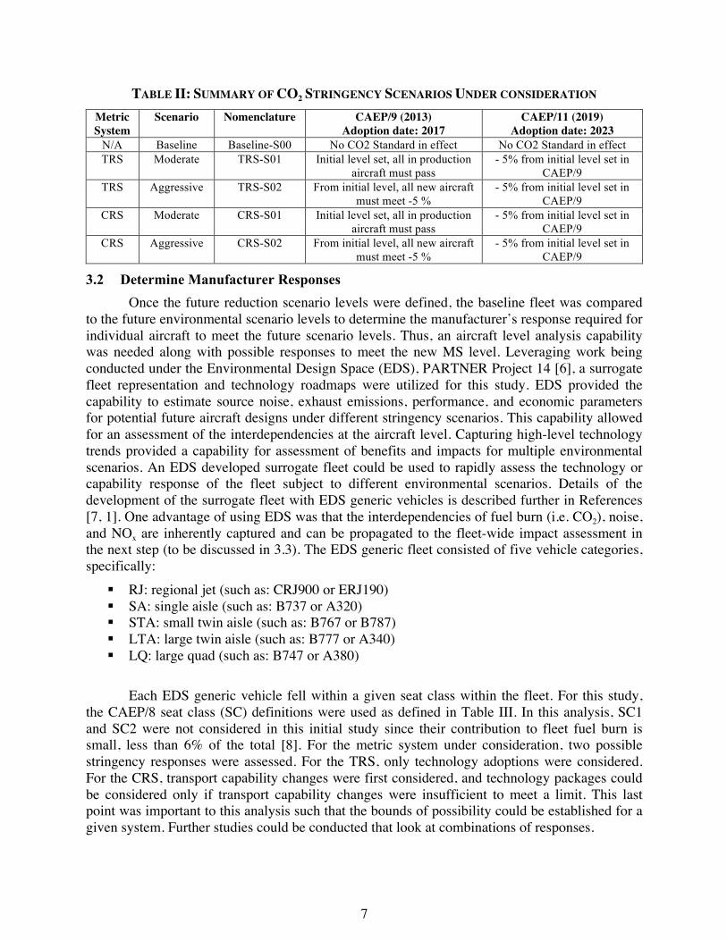
Several types of fits were considered to identify the initial CO2 NLL for the TRS. Since this metric system shows very obvious and simple trends, many of these fits, including linear and second-order fits in absolute, natural log, or log-base-10 space, could be used adequately. For this investigation, a second-order fit with natural log transformations was selected for its qualities and performance and then transformed back to real values so as to move the initial fit for future stringency levels. First, it was evident that a single line could easily be used to

16

approximate the performance of the entire fleet, allowing the benefits of a simple framework to be used. Furthermore, this fit separated in and out of production vehicles very well, which is a desirable characteristic of a good metric system and associated initial limit line. Finally, the behavior of individual aircraft with respect to a margin also fell within logical reasoning of technology differences between aircraft types. The initial CO2 limit line for the TRS is depicted in Figure 7 and shows out of production aircraft, in production aircraft, the baseline EDS aircraft, and the initial TRS CO2 limit line.

0.0

2.0

4.0

6.0

8.0

10.0

12.0

14.0

0 100,000 200,000 300,000 400,000 500,000

1/SA

R (k

g/km

)

(MTOW+MZFW)/2 (kg)

Out of Production In Production EDS Baseline Vehicles Initial CAEP/9 Level

FIGURE 7: INITIAL CO2 METRIC SYSTEM LEVEL FOR THE TRS

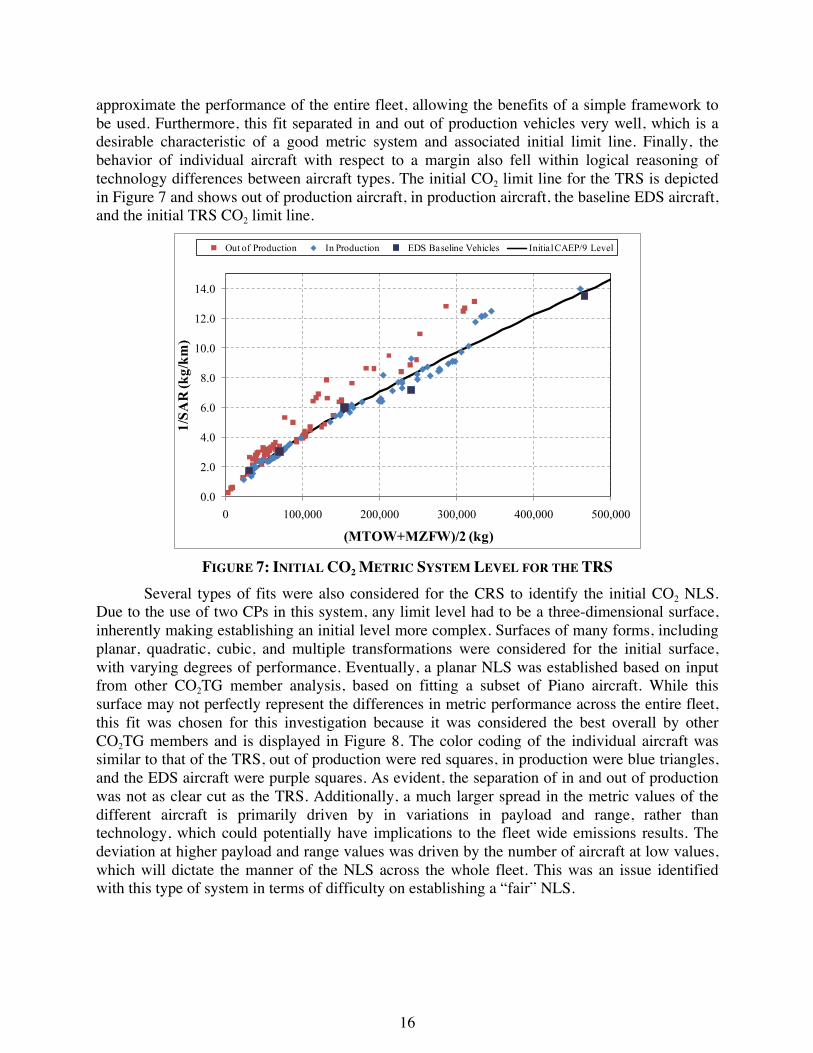
Several types of fits were also considered for the CRS to identify the initial CO2 NLS. Due to the use of two CPs in this system, any limit level had to be a three-dimensional surface, inherently making establishing an initial level more complex. Surfaces of many forms, including planar, quadratic, cubic, and multiple transformations were considered for the initial surface, with varying degrees of performance. Eventually, a planar NLS was established based on input from other CO2TG member analysis, based on fitting a subset of Piano aircraft. While this surface may not perfectly represent the differences in metric performance across the entire fleet, this fit was chosen for this investigation because it was considered the best overall by other CO2TG members and is displayed in Figure 8. The color coding of the individual aircraft was similar to that of the TRS, out of production were red squares, in production were blue triangles, and the EDS aircraft were purple squares. As evident, the separation of in and out of production was not as clear cut as the TRS. Additionally, a much larger spread in the metric values of the different aircraft is primarily driven by in variations in payload and range, rather than technology, which could potentially have implications to the fleet wide emissions results. The deviation at higher payload and range values was driven by the number of aircraft at low values, which will dictate the manner of the NLS across the whole fleet. This was an issue identified with this type of system in terms of difficulty on establishing a “fair” NLS.

17

MF/

D at

40%

Rm

ax(k

g/km

)

FIGURE 8: INITIAL CO2 METRIC SYSTEM LEVEL FOR THE CRS

The NLL/S equation for each metric system is provided below. The TRS CO2 equation is rather unique. The rationale behind having natural log coefficients and then taking the exponential of the value is to account for the scale effects of increasing aircraft size. This allows for a percent change from the baseline metric values as the CP increases to allow for equal technology responses across aircraft types when the percentage is applied to the absolute value.

MaxPayload Rmax@50%*840.00008013MaxPayload*680.0000830770.486893962_2_ )MZFW))(MTOW*(*0.5*3024420.00298767MZFW)(MTOW*0.5*639082383Ln(0.71917068648)-7.2710009(( 2

++=

= ++++

COCRSeCOTRS Ln

As a hypothesis by the research team, the placement of the initial CO2 limit level on each

metric system could have a large impact on the final fleet-wide CO2 emissions, because the limit line determines the degree to which each EDS generic vehicle will have to respond to meet a given stringency. For instance, in the TRS, the SA, LTA, and LQ aircraft fell below the initial line, which should be expected since the aircraft are newer technology and are more fuel efficient than their counterparts. Meanwhile, the RJ and STA fall above the line, due to their older technology, a result which also makes logical sense. In this manner, the placement of the initial line for TRS required the addition of technology in an expected and reasonable manner rather than changes in transport capability, which should be reflected in the cumulative fleet-level CO2 emissions. As such, the TRS would appear to be transport capability neutral and promote the adoption of technology to meet future stringency levels.

The limit level defined for the CRS could have a large impact on fleet-wide emissions. With this metric system and limit surface, the location of the EDS generic vehicles with respect to the surface was opposite of the TRS. For example, the LQ fell well above the surface by a large margin and the RJ fell well below the surface. This is counter to the author’s expectations of where this specific aircraft should fall with respect to a margin and implies that significant

18

changes had to be made to aircraft in a different fashion than in TRS. Due to the properties of CRS being highly sensitive to transport capability, a possible response to a new stringency would obviously be changes in payload or range, rather than technology adoption. This observation would suggest that this system is not neutral to changes in transport capability, but rather, promotes capability changes instead of technology adoption. Thus, due to the placement of the initial limit levels and differing amounts of technological progress required, this investigation from the outset suggests that the cumulative fleet-level CO2 emissions from both metric systems will be quite different. However, since a number of CO2TG members believed this was an adequate limit level for this metric system, the authors will utilize it for the stringency scenarios. Lastly, under the assumptions for this study a TRS versus a CRS would imply different responses to a given stringency scenario and as such, bound and quantify the system wide implications of those assumptions. Future studies can consider deviations from these assumptions.

4.1.3 Moderate Response Scenario Definition (S01) The premise behind the moderate response scenario (S01) was a slow progression of CO2

advances that would not significantly affect current manufacturer production lines, but follow the anticipated progression of the fleet. As mentioned previously, the first adoption of an improvement over the baseline level for this scenario would occur at a moderate level in 2017 and become more aggressive as time moves on. Thus, most of the aircraft in the fleet would have more than a decade to respond to a stricter CO2 level. This corresponds to the general trend seen in commercial aerospace systems, where approximately 7 to 15 years from concept formulation until the product launch date is required [19], as discussed in prior sections with the historical trends in margins.

To ensure a slow progression, the initial CO2 limit described above was used as the initial limit that aircraft had to pass at the assumed introduction of the standard in 2017. This methodology required no technological advances from the best performers, and only affected the worst performers in the fleet. For modeling purposes, this initial trend was assumed to be approved in the CAEP/9 cycle, with a limit adoption date of 2017 and an introduction for fleet operations in 2018. An update of this limit was then required for the following cycle, CAEP/11, assumed to be adopted in 2023, with an introduction in 2024. In order to define the updated TRS level for S01, an iterative scheme was utilized that lowered the initial CO2 MS level and tracked the specific aircraft in the fleet that failed based on the certification date and class of the given aircraft.

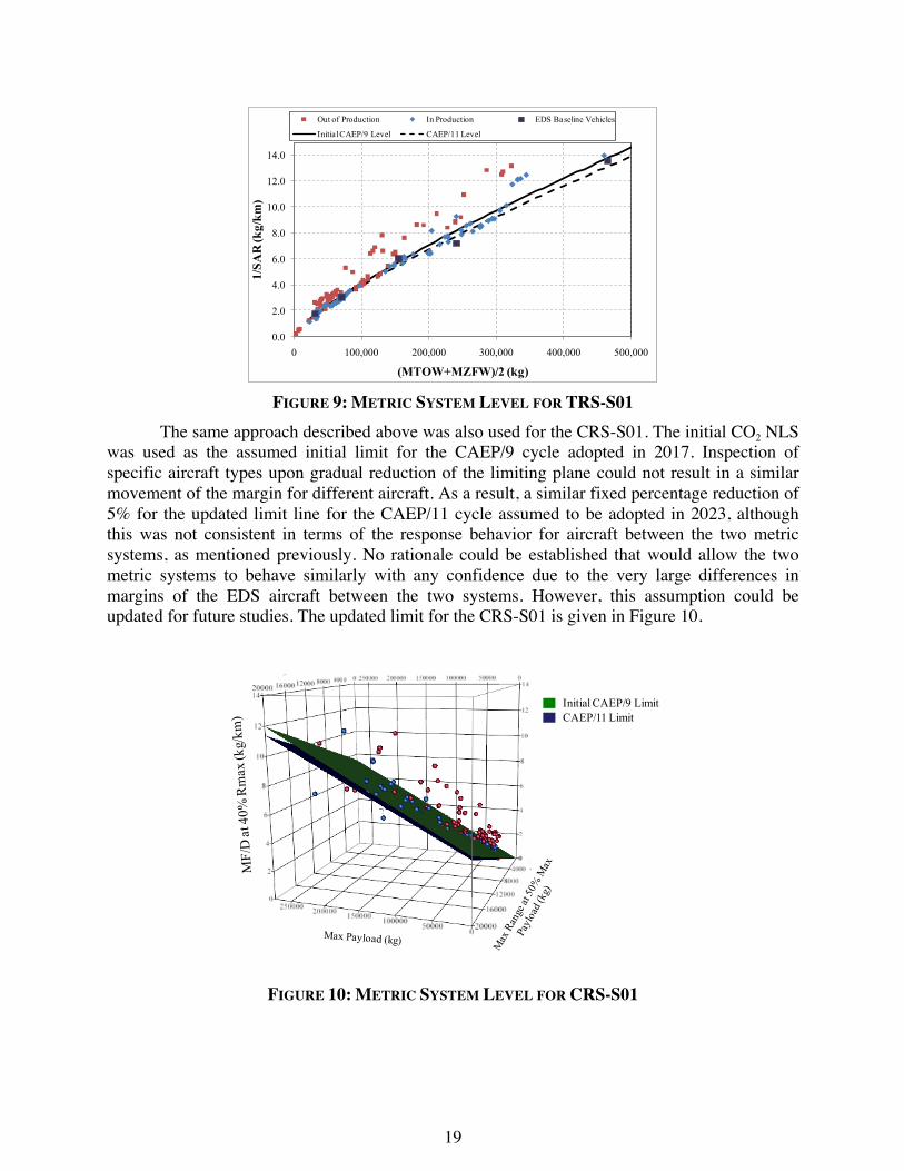
As a general rule for reducing the baseline trend, preference was given to levels which affected older certification dates first, essentially allowing the limit to first target aircraft with the oldest technology and thus poorest fuel efficiency. By affecting these older aircraft as the first to fail a limit, the scenarios in this study enabled older and less efficient aircraft to be the first to be replaced with newer technology. Preference was also given to levels which were not significantly biased toward any aircraft class, and affected all aircraft classes approximately equivalently. By inspecting which specific aircraft began to fail the limit as it was gradually reduced, and leveraging insight from the EDS technology roadmaps as to anticipated near-term technologies, it was determined that a fixed percentage reduction of 5% from the initial limit was reasonable for the updated limit. This updated limit is depicted for the TRS-S01 in Figure 9.

19

0.0

2.0

4.0

6.0

8.0

10.0

12.0

14.0

0 100,000 200,000 300,000 400,000 500,000

1/SA

R (k

g/km

)

(MTOW+MZFW)/2 (kg)

Out of Production In Production EDS Baseline Vehicles

Initial CAEP/9 Level CAEP/11 Level

FIGURE 9: METRIC SYSTEM LEVEL FOR TRS-S01

The same approach described above was also used for the CRS-S01. The initial CO2 NLS was used as the assumed initial limit for the CAEP/9 cycle adopted in 2017. Inspection of specific aircraft types upon gradual reduction of the limiting plane could not result in a similar movement of the margin for different aircraft. As a result, a similar fixed percentage reduction of 5% for the updated limit line for the CAEP/11 cycle assumed to be adopted in 2023, although this was not consistent in terms of the response behavior for aircraft between the two metric systems, as mentioned previously. No rationale could be established that would allow the two metric systems to behave similarly with any confidence due to the very large differences in margins of the EDS aircraft between the two systems. However, this assumption could be updated for future studies. The updated limit for the CRS-S01 is given in Figure 10.

Initial CAEP/9 LimitCAEP/11 Limit

FIGURE 10: METRIC SYSTEM LEVEL FOR CRS-S01

20

While S01 was designed to represent gradual progression of CO2 emissions in the fleet, the assumed adoption of the limits in the CAEP/9 and CAEP/11 cycles resulted in some aircraft failing the limit. In CAEP/9 for both metric systems, the initial limit would need to be met by all aircraft and then the stringency would increase in CAEP/11 to promote further CO2 improvements. In this analysis, aircraft that failed the limit were required to adopt some sort of performance improvement to enable passing the limit, so the aircraft could continue to be produced. As explained earlier, EDS generic vehicles were used in this analysis to represent the current fleet, and as such, generic vehicle performance was investigated with respect to the NLL/S to determine their ability to pass the limit.

Comparison of baseline EDS generic vehicle performance to the CO2 limits in S01 resulted in the margins listed in Table IV. Here, positive values indicate the vehicle performance was above the limit line and failed, while negative values indicate performance was below the limit and the vehicle passed. As is observed, the SA, LTA, and LQ passed the initial CAEP/9 limit in TRS-S01, while only the LTA passed the updated CAEP/11 limit. Very different results were observed in CRS-S01, where the RJ, SA, and LTA pass both CAEP/9 and CAEP/11 limits, while the STA and LQ fail both by very large margins, which is counter-intuitive when the technology levels are compared between vehicles.

This behavior indicates that completely different responses were required between the two systems. For example, in the TRS-S01, the LQ meets the initial stringency by a limited amount and then requires approximately 3% improvements in 2023. Based on the fact that the EDS LQ is representative of an Airbus A380, one of the newest aircraft in the fleet, this response seems reasonable. However with the CRS-S01, the LQ fails the initial stringency by more than 30%. Within the time frames under consideration here, there was no possible way in which a LQ could adopt that level of technology improvements based on the technology packages identified earlier. As such, a change in transport capability could be the only viable option to comply with the limit.

The unusually poor margin of the current-technology LQ aircraft is due to the nature of the CRS system, the vastly greater payload of this aircraft compared to the fleet, and the functional form of the NLS used. Although a planar surface was used to represent the limit in the CRS system, the fact that the LQ representing current technology was such a large outlier suggests that performance of the CRS defined in this study does not vary linearly with respect to the payload and range CPs. The use of other functional forms sometimes yielded more reasonable performance of the LQ with respect to its margin, but at the cost of less reasonable margins elsewhere in the fleet. The difficulty of defining a simple limit line that yields reasonable margins of aircraft across the fleet strongly supports the observation that the non-TCN nature of the CRS system.

21

TABLE IV: EDS BASELINE VEHICLE MARGINS FOR S01 Metric System

Scenario CAEP/9 (2013)

Adoption date: 2017 CAEP/11 (2019)

Adoption date: 2023 TRS-S01 RJ 6.91%

SA -2.27% STA 4.27% LTA -12.02% LQ -1.87%

RJ 12.54% SA 2.87% STA 9.76% LTA -7.39% LQ 3.29%

CRS-S01 RJ -10.34% SA -9.77% STA 11.55% LTA -8.05% LQ 30.70%

RJ -5.62% SA -5.02% STA 17.42% LTA -3.21% LQ 37.58%

4.1.4 Aggressive Scenario Definition (S02) The aggressive scenario (S02) premise was a fast progression of CO2 reduction advances

that would penetrate the fleet quicker. This scenario considered the influence of faster adoption of CO2 metric system level improvements by assuming that the current fleet needed to meet the level set forth in S01 for the 2023 adoption but now in 2017. Subsequently, a further improvement in the metric would be needed in 2023. The anticipated result of this scenario was the influence of more aggressive CO2 framework adoption and its affect on the NAS fuel burn performance. As mentioned previously, the costs associated with the adoption of technology were not considered which would have an impact under this scenario in terms of a cost-benefit analysis.

As stated, the initial limit in 2017 for S02 for both metric systems was assumed to be the limit from moderate scenario set in 2023. Since the same limit is used in both scenarios, its use in 2023 (CAEP/11) in S01 represented more gradual progression, while its use in 2017 (CAEP/9) in S02 represented more aggressive emissions reduction adoption. A further update of the limit was then assumed for the CAEP/11 cycle for this scenario. Using a similar methodology as used previously, the limit was gradually decreased and the specific aircraft that began to fail were inspected in an iterative manner. As a result of this process, it was determined again that a further fixed percentage reduction of 5% was reasonable for the TRS-S02. Similar to before, this also translates to CAEP/11 levels being 5% below CAEP/9 levels. The reduction from the initial limit to the CAEP/9 level and the further reduction to the CAEP/11 limit for the TRS- S02 are shown in Figure 11. This process was repeated once more to find an appropriate level for the CAEP/11 cycle for CRS-S02. It was determined that a fixed percentage reduction of 5% for the NLS was also reasonable for this metric system to attempt to keep an apples to apples comparison for the updated CAEP/11 (2023) limit. However, as noted before, this assumption could be updated in future analysis. The series of NLS for CRS-S02 is depicted in Figure 12.

22

0.0

2.0

4.0

6.0

8.0

10.0

12.0

14.0

0 100,000 200,000 300,000 400,000 500,000

1/SA

R (k

g/km

)

(MTOW+MZFW)/2 (kg)

Out of Production In Production EDS Baseline Vehicles

Initial CO2 Level CAEP/9 Level CAEP/11 Level

FIGURE 11: METRIC SYSTEM LEVEL FOR TRS-S02

MF/

D at

40%

Rm

ax(k

g/km

)

Initial CAEP/9 LimitCAEP/10 LimitCAEP/11 Limit

FIGURE 12: METRIC SYSTEM LEVEL FOR CRS-S02

The margins for both metric systems are provided in Table V. As expected, the more

aggressive scenarios resulted in more vehicles failing the CO2 emission limits, and by a larger degree, requiring more substantial performance enhancements to enable those vehicles to pass. As with S01, the CRS required fairly large improvements to the STA and also the LQ. Additionally, for the 2023 adoption, the LTA failed the CRS limit whereas the RJ and the SA passed. This is counter-intuitive to the technology levels of the given aircraft and appears to be a product of the metric system itself.

23

TABLE V: EDS BASELINE VEHICLE MARGINS FOR S02 Metric System

Scenario CAEP/9 (2013)

Adoption date: 2017 CAEP/11 (2019)

Adoption date: 2023 TRS-S02 RJ 12.54%

SA 2.87% STA 9.76% LTA -7.39% LQ 3.29%

RJ 18.46% SA 8.28% STA 15.54% LTA -2.52% LQ 8.73%

CRS-S02 RJ -5.62% SA -5.02% STA 17.42% LTA -3.21% LQ 37.58%

RJ -0.66% SA -0.02% STA 23.6% LTA 1.89% LQ 44.82%

4.2 Stringency Scenario Manufacturer Responses The next step was to determine the manufacturer’s response that was required to meet

each of the stringency scenarios for the two metric systems. For vehicles that failed a stringency limit, its performance had to be enhanced in some way to enable it to meet the limit. For a typical CAEP stringency analysis, such an enhancement would be the adoption technologies to reduce CO2 emissions, such as the case with the TRS. However, since this investigation includes a non-TCN metric system in the form of the CRS, such that other manufacturer responses were also included, since they may represent less costly and thus more desirable respones. As mentioned previously, a series of analyses with EDS was conducted for changes in technology packages for different time frames of availablity and also changes in transport capability. This effort was conducted in order to establish a set of data for which each metric system would have different possiblities for response aircraft, either technology or capability. Each of these analyses is described further below. 4.2.1 Possible Technology Response Aircraft for the TRS

For determing the appropriate technology response for the TRS scenarios, the EDS generic vehicles and the technology roadmaps previously described were used. The first step in this process was to calculate the metric values for the technology packages available for the different times frames of interest for a typical and aggressive development schedule. The roadmaps utilized to define the aviailable technologies are provided in Appendix A. For both roadmaps, a series of packages were established for each EDS vehicle and are shown in Figure 13 for the typical roadmap and Figure 14 for the aggressive roadmap based on research previously conducted in Ref. [1]. Additionally, based on research conducted by GT for the FAA and Environmental Protection Agency (EPA) [20], a series of packages for produciton line changes were also leveraged for this current research and are provided in Figure 15.

One should note that the advantage of utilizing EDS for the technology responses allows the quantification of the interdependencies of technology adoption and seamless process of propagation of that response through AEDT and GREAT. For example, the adoption of natural laminar flow technology provides not only fuel burn benefits, but noise benefits due to the fact that reduced mission fuel burn also reduces the MTOW of the aircraft for a given payload and range capability, requiring less thrust and producing less noise. This type of simultaneous benefit is common for many fuel burn technologies, and both fuel burn and noise impacts can be quantified with EDS.

24

TYPICAL

Technologies RJ

SA STA

LTA

LQ RJ

SA STA

LTA

LQ

Retro-Fit Winglet and planar wing tipsRetro-Fit Alternate non-planar wing tipsMetallic TechnologiesComposite TechnologiesStructural Health MonintoringNanotechnologiesMultifunctional StructuresAdaptive Wing/Variable CamberShock BumpsMorphing WingNatural Laminar Flow ControlHybrid Laminar Flow ControlDiscrete Roughness ElementsActive TS ControlActive Control for Turbulent Drag ReductionRibletsExcrescence ReductionGeared Turbo Fan (GTF)Active coolingZero Hub FanHighly Loaded CompressorHighly Loaded TurbineMMC (comp)PMC (fan case)PMC with High Temperature Erosion CoatingsCMC (LP HP vanes)Laser/Electron/Friction Stir WeldingTurbine Active Clearance ControlCompressor Active Clearance ControlAdvanced Turbine Disk AlloysAdvanced TBC (on blades only)HPC Flow ControlTurbine Flow Control

2017 2023

FIGURE 13: AVAILABLE TECHNOLOGY RESPONSE PACKAGES FOR TYPICAL ROADMAP

25

AGGRESSIVE

Technologies RJ

SA STA

LTA

LQ RJ

SA LTA

LTA

LTA

Retro-Fit Winglet and planar wing tipsRetro-Fit Alternate non-planar wing tipsMetallic TechnologiesComposite TechnologiesStructural Health MonintoringNanotechnologiesMultifunctional StructuresAdaptive Wing/Variable CamberShock BumpsMorphing WingNatural Laminar Flow ControlHybrid Laminar Flow ControlDiscrete Roughness ElementsActive TS ControlActive Control for Turbulent Drag ReductionRibletsExcrescence ReductionGeared Turbo Fan (GTF)Active coolingZero Hub FanHighly Loaded CompressorHighly Loaded TurbineMMC (comp)PMC (fan case)PMC with High Temperature Erosion CoatingsCMC (LP HP vanes)Laser/Electron/Friction Stir WeldingTurbine Active Clearance ControlCompressor Active Clearance ControlAdvanced Turbine Disk AlloysAdvanced TBC (on blades only)HPC Flow ControlTurbine Flow Control

20232017

FIGURE 14: AVAILABLE TECHNOLOGY RESPONSE PACKAGES FOR AGGRESSIVE ROADMAP

Technologies RJ SA STA LTA LQ Winglets Y Y Y Riblets Y Y Y Y Y Drooped aileron Y Y Y Y Y Lighter cabin furnishing Y Y Y Y Y Re-engine Y Y Y Y

FIGURE 15: TECHNOLOGY RESPONSE PACKAGES FOR PRODUCTION LINE CHANGES

26

As the 2017 and 2023 technology packages were applied to each EDS vehicle, the engine cycle and airframe size were allowed to vary to fully take advantage of the benefits of the technology packages, potentially providing additional environmental benefit beyond additive impacts. Aircraft thrust to weight, wing loading, and fuselage size were held constant while wing and tail surfaces were allowed to scale to meet the aircraft’s mission requirements at the design point (R2, see Figure 1 for reference) for the technology response package results. Advanced engine cycles were chosen from a survey of advanced engines projected to enter service in the two introduction dates mentioned above. Additional mechanical modifications to the engine were modeled in order to account for the geared turbofan (GTF) technology. Note, GTF was only assumed to be applicable to the RJ and SA at the time of this study since it was unclear whether or not a GTF could be scaled to higher thrust levels within the time frame of the scenarios considered herein. In addition, natural laminar flow was applied to the RJ and SA, while hybrid laminar flow was applied to the larger aircraft (STA, LTA, and LQ). Also, an advanced combustor was also applied to each aircraft so as to meet the current CAEP/8 and future NOx stringency levels. This is an important assumption that drives the fleet-wide NOx results as will be discussed in later sections.

For the production line changes, all aspects of the aircraft were held constant except for the specific technology being added. For example, the addition of the winglets were simulated by an increase in wing weight and improvement in the aerodynamcs. All other aspects of the aircraft were fixed. The final production line change packages were selected based on which packages minimized fuel burn, with no consideration of NOx or noise. However, an advanced combustor was also applied to each aircraft so as to meet the current CAEP/8 and future NOx stringency levels.

The baseline 1/SAR values along with the percent change from the baseline for each of the packages is listed in Table VI. An interesting result occurred for most of the vehicles for the production line changes versus the packages available in 2017. Most production line changes actually had more improvement in 1/SAR. In comparing the packages between the two, the main difference was the addition of the riblets, drooped aileron, and the lighter cabin furnishing for the production line changes. All production line changes, excluding the LQ, all had a re-engine, which was also used on the 2017 and 2023 packages. When comparing these changes to the roadmap technologies, a few aerodynamic technologies were swapped out between the two approaches, but all had re-engines. For the 2017 and 2023 packages, all of the aircraft added composites, but the swapping of the aerodnamic technologies provided the large benefit than the weight reduction. The primary difference in the impacts of the packages resulted from the production line technologies being chosen to minimize fuel burn, whereas the 2017 and 2023 packages where based on a balanced solution that attempted to minimize fuel burn, NOx, and noise concurrently.

The simplified mission fuel burn for each aircraft at the design point (R2, see Figure 1 for reference) is also provided in Table VII. For each aircraft, the percent change between 1/SAR and mission fuel at the design point were within a few percent, which implied that a change in the single point metric was similar to a full mission metric. These technology package results provided a basis for the aircraft responses to for the TRS stringency scenarios.

27

TABLE VI: 1/SAR COMPARISONS FOR POTENTIAL TECHNOLOGY RESPONSES, BASELINE AND PERCENT CHANGE FROM BASELINE

Package RJ SA STA LTA LQ Baseline (kg/km) 1.745 3.016 5.994 7.191 12.898

Prod Line Tech Response -14.46% -11.19% -16.11% -12.08% -4.71% 2017 Typical -14.21% -9.38% -16.04% -12.95% -9.81% 2023 Typical -24.16% -27.11% -33.05% -27.02% -25.48%

2017 Aggressive -17.66% -18.45% 24.58% -19.22% -17.20% 2023 Aggressive -28.47% -31.02% -38.04% -32.35% -29.75%

TABLE VII: MF AT R2 COMPARISONS FOR POTENTIAL TECHNOLOGY RESPONSES, BASELINE AND PERCENT CHANGE FROM BASELINE

Package RJ SA STA LTA LQ Baseline (kg) 6803 17034 68074 111985 202558 Prod Line Tech Response -14.34% -13.34% -15.49% -14.56% -4.49% 2017 Typical -14.13% -12.43% -16.57% -15.80% -10.13% 2023 Typical -24.46% -29.15% -33.48% -27.45% -25.86% 2017 Aggressive -17.38% -18.60% -24.65% -21.37% -17.63% 2023 Aggressive -28.82% -33.43% -38.58% -33.22% -30.64%

4.2.2 Possible Capability Response Aircraft for the CRS Alternative manufacturer responses to a CO2 emission stringency included in this

research were changes in aircraft transport capability (TC), namely payload and range. These alternate aircraft were investigated for their anticipated use in a metric system that is not TCN, such as the CRS considered herein. In short, the EDS generic vehicles were resized for combinations of higher and lower payload and range variants. These vehicles were used both to test whether each metric system was TCN, as well as to provide candidate responses to the CRS scenarios. As defined previously, a TCN system should yield approximately equal margins for aircraft of simialar technology level but differing transport capabilities.

For the current study, TC variants of the baseline EDS generic vehicles were developed by increasing or decreasing design payload and range independently and in combinations. The excursions from the baseline design point which constituted the basic TC variant design is depicted in Figure 16. The nomenclature for each of these re-designed points is provided in Table VIII. For the “H” value of payload or range, a +15% increase from the design point was assumed. In contrast, for the “L” value of payload or range, a -15% increase from the design point was assumed TC variants were resized to meet the new design condition for each case and the engines were scaled accordingly. The fuselage was assumed to be lengthened or shortened appropriately for a larger or smaller payload, respectively. To test alternative assumptions, several cases including higher and lower payload and range but keeping the same fuselage geometry as the baseline were also included to determine if the manner in which payload is utilized on the aircraft would matter with respect to the margin. These special cases are also included in Table VIII. Also, an advanced combustor was also applied to each aircraft so as to meet the current CAEP/8 and future NOx stringency levels.

28

Payl

oad

Range

Notional Payload-Range Diagram

Payload-Range EnvelopeDesign Point

Transport Capability Changes

FIGURE 16: DEFINITION OF EDS TRANSPORT CAPABILITY CHANGES

TABLE VIII: EDS TRANSPORT CAPABILITY CHANGE NOMENCLATURE

TC Variant Payload Range Fuselage Length

HH High High Lengthened HL High Low Lengthened HB High Baseline Lengthened HB_basefuselage High Baseline Baseline BH Baseline High Baseline BL Baseline Low Baseline LH Low High Shortened LL Low Low Shortened LB Low Baseline Shortened LB_basefuselage Low Baseline Baseline

As with the TRS, the CRS metric system values were calculated with EDS for each of the

potential TC responses. The MF/D metric results are provided in Table IX and the changes in MF at the design point are listed in Table X. An interesting observation was made between the change in the metric value, MF/D, and the actual fuel burn at R2. Unlike the TRS, the direction of change of the metric and the fuel burn were not in the same direction. For example, the RJ at the high payload and low range (HL) increased in value of the metric from the baseline but actually reduced for the fuel burn. Additionally, the order of magnitude of the change of the TC variants from the baseline were on the order of, if not larger than, the changes from the technology packages for the TRS. For example, the LTA HH had a 22.27% change in the metric and a 40.09% change in MF from the baseline. For the TRS, the LTA 2023 aggressive package could only provide approximately 33% change in both metric and MF. These results reconfirm prior observations regarding the CRS metric system’s sensitivity to changes in transport capability and the influence on the metric and potentially the margin to the NLS. For example, the RJ metric variation is approximately 22% between all the derivatives and approximately 33% for the LTA. Given the large variation in the metric from TC changes, this system lends itself to the manufacturer’s responding to a new stringency level simply by changing TC. The response would be an intuitively obvious result given that the manufacturer would limit the cost investment to respond to a CO2 limit.

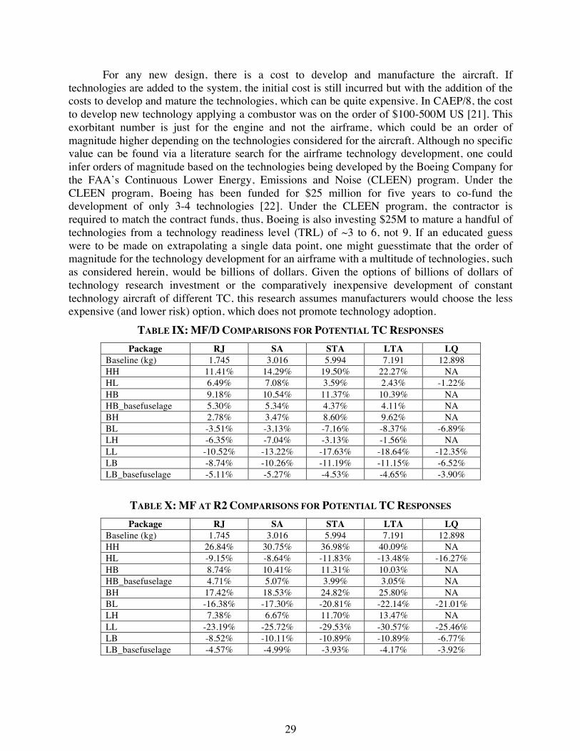
29

For any new design, there is a cost to develop and manufacture the aircraft. If technologies are added to the system, the initial cost is still incurred but with the addition of the costs to develop and mature the technologies, which can be quite expensive. In CAEP/8, the cost to develop new technology applying a combustor was on the order of $100-500M US [21]. This exorbitant number is just for the engine and not the airframe, which could be an order of magnitude higher depending on the technologies considered for the aircraft. Although no specific value can be found via a literature search for the airframe technology development, one could infer orders of magnitude based on the technologies being developed by the Boeing Company for the FAA’s Continuous Lower Energy, Emissions and Noise (CLEEN) program. Under the CLEEN program, Boeing has been funded for $25 million for five years to co-fund the development of only 3-4 technologies [22]. Under the CLEEN program, the contractor is required to match the contract funds, thus, Boeing is also investing $25M to mature a handful of technologies from a technology readiness level (TRL) of ~3 to 6, not 9. If an educated guess were to be made on extrapolating a single data point, one might guesstimate that the order of magnitude for the technology development for an airframe with a multitude of technologies, such as considered herein, would be billions of dollars. Given the options of billions of dollars of technology research investment or the comparatively inexpensive development of constant technology aircraft of different TC, this research assumes manufacturers would choose the less expensive (and lower risk) option, which does not promote technology adoption.

TABLE IX: MF/D COMPARISONS FOR POTENTIAL TC RESPONSES Package RJ SA STA LTA LQ

Baseline (kg) 1.745 3.016 5.994 7.191 12.898 HH 11.41% 14.29% 19.50% 22.27% NA HL 6.49% 7.08% 3.59% 2.43% -1.22% HB 9.18% 10.54% 11.37% 10.39% NA HB_basefuselage 5.30% 5.34% 4.37% 4.11% NA BH 2.78% 3.47% 8.60% 9.62% NA BL -3.51% -3.13% -7.16% -8.37% -6.89% LH -6.35% -7.04% -3.13% -1.56% NA LL -10.52% -13.22% -17.63% -18.64% -12.35% LB -8.74% -10.26% -11.19% -11.15% -6.52% LB_basefuselage -5.11% -5.27% -4.53% -4.65% -3.90%

TABLE X: MF AT R2 COMPARISONS FOR POTENTIAL TC RESPONSES Package RJ SA STA LTA LQ

Baseline (kg) 1.745 3.016 5.994 7.191 12.898 HH 26.84% 30.75% 36.98% 40.09% NA HL -9.15% -8.64% -11.83% -13.48% -16.27% HB 8.74% 10.41% 11.31% 10.03% NA HB_basefuselage 4.71% 5.07% 3.99% 3.05% NA BH 17.42% 18.53% 24.82% 25.80% NA BL -16.38% -17.30% -20.81% -22.14% -21.01% LH 7.38% 6.67% 11.70% 13.47% NA LL -23.19% -25.72% -29.53% -30.57% -25.46% LB -8.52% -10.11% -10.89% -10.89% -6.77% LB_basefuselage -4.57% -4.99% -3.93% -4.17% -3.92%

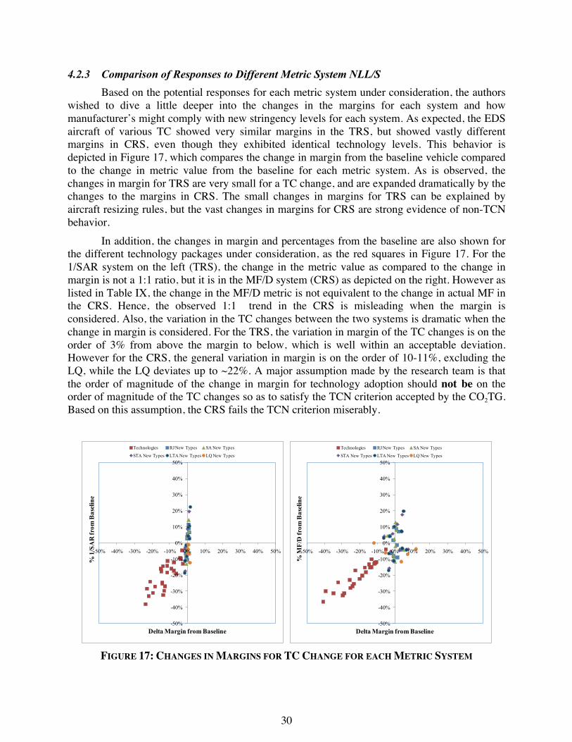
30

4.2.3 Comparison of Responses to Different Metric System NLL/S Based on the potential responses for each metric system under consideration, the authors

wished to dive a little deeper into the changes in the margins for each system and how manufacturer’s might comply with new stringency levels for each system. As expected, the EDS aircraft of various TC showed very similar margins in the TRS, but showed vastly different margins in CRS, even though they exhibited identical technology levels. This behavior is depicted in Figure 17, which compares the change in margin from the baseline vehicle compared to the change in metric value from the baseline for each metric system. As is observed, the changes in margin for TRS are very small for a TC change, and are expanded dramatically by the changes to the margins in CRS. The small changes in margins for TRS can be explained by aircraft resizing rules, but the vast changes in margins for CRS are strong evidence of non-TCN behavior.

In addition, the changes in margin and percentages from the baseline are also shown for the different technology packages under consideration, as the red squares in Figure 17. For the 1/SAR system on the left (TRS), the change in the metric value as compared to the change in margin is not a 1:1 ratio, but it is in the MF/D system (CRS) as depicted on the right. However as listed in Table IX, the change in the MF/D metric is not equivalent to the change in actual MF in the CRS. Hence, the observed 1:1 trend in the CRS is misleading when the margin is considered. Also, the variation in the TC changes between the two systems is dramatic when the change in margin is considered. For the TRS, the variation in margin of the TC changes is on the order of 3% from above the margin to below, which is well within an acceptable deviation. However for the CRS, the general variation in margin is on the order of 10-11%, excluding the LQ, while the LQ deviates up to ~22%. A major assumption made by the research team is that the order of magnitude of the change in margin for technology adoption should not be on the order of magnitude of the TC changes so as to satisfy the TCN criterion accepted by the CO2TG. Based on this assumption, the CRS fails the TCN criterion miserably.

-50%

-40%

-30%

-20%

-10%

0%

10%

20%

30%

40%

50%

-50% -40% -30% -20% -10% 0% 10% 20% 30% 40% 50%

% 1

/SA

R fr

om B

asel

ine

Delta Margin from Baseline

Technologies RJ New Types SA New Types

STA New Types LTA New Types LQ New Types

-50%

-40%

-30%

-20%

-10%

0%

10%

20%

30%

40%

50%

-50% -40% -30% -20% -10% 0% 10% 20% 30% 40% 50%

% M

F/D

from

Bas

elin

e

Delta Margin from Baseline

Technologies RJ New Types SA New Types

STA New Types LTA New Types LQ New Types

FIGURE 17: CHANGES IN MARGINS FOR TC CHANGE FOR EACH METRIC SYSTEM

31

It should be noted that the margins in Figure 17 are in reference to the functional form and placement of the stringency limits, and would change if the limit defined by the NLL or NLS were established differently. However, research by the Project 30 team has shown that non-TCN is a property of this MF/D metric system as a whole due to the inclusion of payload and range terms, which cannot be corrected by assuming a different slope or form of the limit line. Therefore, for this research, TRS is considered TCN and CRS is considered non-TCN. This conclusion also means that TC changes are viable options in CRS for improving aircraft score to a limit and included this research as potential manufacturer responses for compliance with a standard. Because the TRS is TCN, changes in aircraft TC have no effect on the margin, meaning technology addition is the only viable manufacturer response. 4.2.4 TRS Manufacturer Response

For each TRS scenario, two dates of introduction were assumed: 2017 and 2023, which implies an introduction of 2018 and 2024 respectively. Each technology package was applied to the EDS generic vehicles and the environmental metrics (noise, 1/SAR, and NOx) were tabulated and compared to the different scenario level requirements, as described previously. For each scenario and adoption date, the most appropriate package was determined for each EDS generic vehicle by choosing the minimal set of technologies required to meet the given CO2 metric system scenario level at a given adoption date. Again, the rationale behind this approach was based on the fact that the development of technologies requires a significant investment and manufacturers would choose solutions with a fewer number of technologies, assuming that more technologies require more investment. Based on this approach and the supporting data, the packages listed in Table XI and the specific technologies identified in Section 4.2.1 were selected as the TRS response and used to assess the fleet-wide environmental impacts.

TABLE XI: TECHNOLOGY RESPONSES FOR TRS-S01 AND TRS-S02 Scenario 2017 Adoption 2023 Adoption

Seat Class

Replacement Type Response Type Seat

Class Replacement

Type Response Type

TRS-S01

RJ: SA: STA: LTA: LQ:

EDS RJ EDS SA EDS STA EDS LTA EDS LQ

In-Prod. Tech Baseline In-Prod. Tech Baseline Baseline

RJ: SA: STA: LTA: LQ:

EDS RJ EDS SA EDS STA EDS LTA EDS LQ

In-Prod. Tech In-Prod. Tech In-Prod. Tech Baseline 2017 Typical

TRS-S02

RJ: SA: STA: LTA: LQ:

EDS RJ EDS SA EDS STA EDS LTA EDS LQ

In-Prod. Tech In-Prod. Tech In-Prod. Tech Baseline 2017 Typical

RJ: SA: STA: LTA: LQ:

EDS RJ EDS SA EDS STA EDS LTA EDS LQ

2023 Typical In-Prod. Tech In-Prod. Tech Baseline 2023 Typical

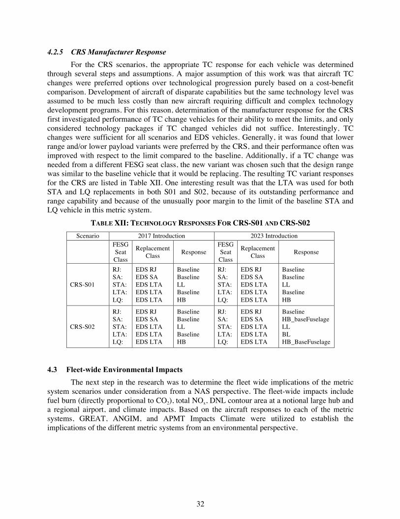
32

4.2.5 CRS Manufacturer Response For the CRS scenarios, the appropriate TC response for each vehicle was determined

through several steps and assumptions. A major assumption of this work was that aircraft TC changes were preferred options over technological progression purely based on a cost-benefit comparison. Development of aircraft of disparate capabilities but the same technology level was assumed to be much less costly than new aircraft requiring difficult and complex technology development programs. For this reason, determination of the manufacturer response for the CRS first investigated performance of TC change vehicles for their ability to meet the limits, and only considered technology packages if TC changed vehicles did not suffice. Interestingly, TC changes were sufficient for all scenarios and EDS vehicles. Generally, it was found that lower range and/or lower payload variants were preferred by the CRS, and their performance often was improved with respect to the limit compared to the baseline. Additionally, if a TC change was needed from a different FESG seat class, the new variant was chosen such that the design range was similar to the baseline vehicle that it would be replacing. The resulting TC variant responses for the CRS are listed in Table XII. One interesting result was that the LTA was used for both STA and LQ replacements in both S01 and S02, because of its outstanding performance and range capability and because of the unusually poor margin to the limit of the baseline STA and LQ vehicle in this metric system.

TABLE XII: TECHNOLOGY RESPONSES FOR CRS-S01 AND CRS-S02 Scenario 2017 Introduction 2023 Introduction

FESG Seat Class

Replacement Class Response

FESG Seat Class

Replacement Class Response

CRS-S01

RJ: SA: STA: LTA: LQ:

EDS RJ EDS SA EDS LTA EDS LTA EDS LTA

Baseline Baseline LL Baseline HB

RJ: SA: STA: LTA: LQ:

EDS RJ EDS SA EDS LTA EDS LTA EDS LTA

Baseline Baseline LL Baseline HB

CRS-S02

RJ: SA: STA: LTA: LQ:

EDS RJ EDS SA EDS LTA EDS LTA EDS LTA

Baseline Baseline LL Baseline HB

RJ: SA: STA: LTA: LQ:

EDS RJ EDS SA EDS LTA EDS LTA EDS LTA

Baseline HB_baseFuselage LL BL HB_BaseFuselage

4.3 Fleet-wide Environmental Impacts

The next step in the research was to determine the fleet wide implications of the metric system scenarios under consideration from a NAS perspective. The fleet-wide impacts include fuel burn (directly proportional to CO2), total NOx, DNL contour area at a notional large hub and a regional airport, and climate impacts. Based on the aircraft responses to each of the metric systems, GREAT, ANGIM, and APMT Impacts Climate were utilized to establish the implications of the different metric systems from an environmental perspective.

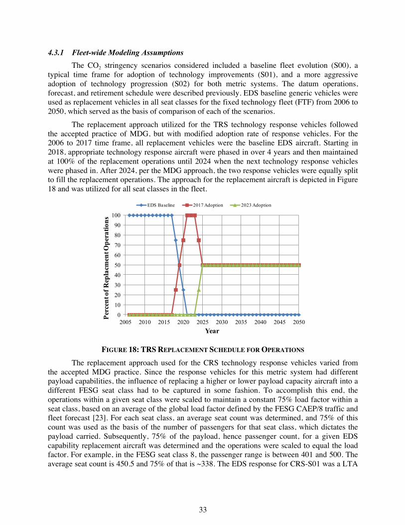
33

4.3.1 Fleet-wide Modeling Assumptions The CO2 stringency scenarios considered included a baseline fleet evolution (S00), a

typical time frame for adoption of technology improvements (S01), and a more aggressive adoption of technology progression (S02) for both metric systems. The datum operations, forecast, and retirement schedule were described previously. EDS baseline generic vehicles were used as replacement vehicles in all seat classes for the fixed technology fleet (FTF) from 2006 to 2050, which served as the basis of comparison of each of the scenarios.

The replacement approach utilized for the TRS technology response vehicles followed the accepted practice of MDG, but with modified adoption rate of response vehicles. For the 2006 to 2017 time frame, all replacement vehicles were the baseline EDS aircraft. Starting in 2018, appropriate technology response aircraft were phased in over 4 years and then maintained at 100% of the replacement operations until 2024 when the next technology response vehicles were phased in. After 2024, per the MDG approach, the two response vehicles were equally split to fill the replacement operations. The approach for the replacement aircraft is depicted in Figure 18 and was utilized for all seat classes in the fleet.

0

10

20

30

40

50

60

70

80

90

100

2005 2010 2015 2020 2025 2030 2035 2040 2045 2050

Perc

ent o

f Rep

lacm

ent O

pera

tions

Year

EDS Baseline 2017 Adoption 2023 Adoption

FIGURE 18: TRS REPLACEMENT SCHEDULE FOR OPERATIONS

The replacement approach used for the CRS technology response vehicles varied from the accepted MDG practice. Since the response vehicles for this metric system had different payload capabilities, the influence of replacing a higher or lower payload capacity aircraft into a different FESG seat class had to be captured in some fashion. To accomplish this end, the operations within a given seat class were scaled to maintain a constant 75% load factor within a seat class, based on an average of the global load factor defined by the FESG CAEP/8 traffic and fleet forecast [23]. For each seat class, an average seat count was determined, and 75% of this count was used as the basis of the number of passengers for that seat class, which dictates the payload carried. Subsequently, 75% of the payload, hence passenger count, for a given EDS capability replacement aircraft was determined and the operations were scaled to equal the load factor. For example, in the FESG seat class 8, the passenger range is between 401 and 500. The average seat count is 450.5 and 75% of that is ~338. The EDS response for CRS-S01 was a LTA

34

with 15% increased payload and the baseline design range, which results in an average seat count of ~302 for a 75% load factor. Thus, the operations in seat class 8 were scaled by the ratio of 338/302, or an increase in operations by a factor of ~1.12. The same rationale was also conducted in seat class 9 which resulted in an operations scale factor of ~1.37, and in seat class 6 the operations were scaled by a factor of ~0.86. All other seat class operations remained the same as the baseline forecast. The replacement schedule for different seat classes is depicted in Figure 19. For seat classes 2-5 and 7, the operations remain unchanged. For seat class 6, the operations are reduced since a high capacity LTA is replacing the baseline STA in the out years. For seat class 8 and 9, the operations increase due to a lower capacity LTA replacing the baseline LQ. The replacement schedule was consistent between CRS-S01 and CRS-S02 due to the nature of the capability response aircraft, as listed in Table XII.

0

10

20

30

40

50

60

70

80

90

100

2005 2010 2015 2020 2025 2030 2035 2040 2045 2050

Perc

ent o

f Rep

lacm

ent O

pera

tions

Year

SC 2-5 and 7 EDS Baseline SC 2-5 and 7 2017 Adoption SC 2-5 and 7 2023 Adoption

0

10

20

30

40

50

60

70

80

90

100

2005 2010 2015 2020 2025 2030 2035 2040 2045 2050

Perc

ent o

f Rep

lacm

ent O

pera

tions

Year

SC 6 EDS Baseline SC 6 2017 Adoption SC 6 2023 Adoption

0

20

40

60

80

100

120

140

2005 2010 2015 2020 2025 2030 2035 2040 2045 2050

Perc

ent o

f Rep

lacm

ent O

pera

tions

Year

SC 8 EDS Baseline SC 8 2017 Adoption SC 8 2023 Adoption

0

20

40

60

80

100

120

140

2005 2010 2015 2020 2025 2030 2035 2040 2045 2050

Perc

ent o

f Rep

lacm

ent O

pera

tions

Year

SC 9 EDS Baseline SC 9 2017 Adoption SC 9 2023 Adoption

FIGURE 19: CRS REPLACEMENT SCHEDULE FOR OPERATIONS

4.3.2 Analysis of CO2 Scenarios The next step in this research was to model the different scenarios under consideration.

For each metric system and stringency scenarios, the necessary data for each of the environmental tools was collected. For GREAT, the necessary data included the replacement schedule and the fuel burn and NOx characteristics for each vehicle as a function of flight distance. ANGIM required the flight schedules for each scenario for the base year and specific out years of interest, and detailed noise grids for a single-event landing and takeoff cycle. Lastly, the APMT Impacts climate module used total fuel burn and NOx by year, from GREAT, for each of the five scenarios. As a reminder to the reader, the five scenarios considered for this research are listed in Table XIII. These scenarios were then assessed using GREAT, ANGIM, and APMT.

35

TABLE XIII: SUMMARY OF CO2 STRINGENCY SCENARIOS UNDER CONSIDERATION Metric System Scenario Nomenclature CAEP/9 (2013)

Adoption date: 2017 CAEP/11 (2019)

Adoption date: 2023 NA Baseline Baseline-S00 No CO2 Standard in effect No CO2 Standard in effect

TRS Moderate TRS-S01 Initial level set, all in production aircraft must pass

- 5% from initial level set in CAEP/9

TRS Aggressive TRS-S02 From initial level, all new aircraft must meet -5 %

- 5% from initial level set in CAEP/9

CRS Moderate CRS-S01 Initial level set, all in production aircraft must pass

- 5% from initial level set in CAEP/9

CRS Aggressive CRS-S02 From initial level, all new aircraft must meet -5 %

- 5% from initial level set in CAEP/9

4.3.2.1 Total Fleet Fuel Consumption The first comparison of this research was the impact to total fleet fuel burn for both

metric systems. The total fuel burn from 2006 to 2050 is depicted in Figure 20 for each of the five scenarios and in Figure 21 as a percent change from the FTF. Fuel burn totals are also listed for particular out-years in Table XIV. For each of the stringency scenarios, the total fuel burn deviates from the FTF starting in 2018 and then further in 2024 when each of the replacement vehicles enters the fleet. The change from the FTF takes a number of years before reductions are obvious since the turnover rate of the fleet is not instantaneous, but takes many years for new and improved aircraft to have a substantial effect and retire out the older, inefficient aircraft.

As expected, the TRS-S02 provides the most benefit in terms of fuel burn reduction due to the aggressive adoption of technology with a total reduction in 2050 of 9.5% over the FTF. The TRS-S01 provides a 5.27% reduction in 2050. Interestingly, both of the capability scenarios also provide a benefit in terms of total fuel burn with CRS-S01 a 2.47% and CRS-S02 a 1.51% reduction. This was an unexpected result that required further investigation, especially since two of the seat classes for these scenarios had increases in the number of operations for both CRS scenarios. It is also interesting that the CRS-S02 shows a benefit over the TRS-S01 for the years 2018-2024, before being eclipsed by TRS benefits in later years. This temporary benefit is an artifact of the forecast and the replacements used, where the assumptions for CRS-S02 replacements happen to have a large impact in some seat classes in the short term near 2018, and then are quickly overtaken by forecasted operations in other seat classes in later years, while the TRS replacements gradually but continually show improvements over time. In general, both TRS scenarios show significant benefit over CRS scenarios in the long term.

36

50

60

70

80

90

100

110

2005 2010 2015 2020 2025 2030 2035 2040 2045 2050

Flee

t Fue

l Bur

n (k

g)B

illio

ns

Year

Baseline FTF TRS-S01 TRS-S02 CRS-S01 CRS-S02

FIGURE 20: TOTAL FLEET FUEL BURN COMPARISON OF CO2 METRIC SYSTEM SCENARIOS

TABLE XIV: FLEET FUEL BURN TOTALS BY INCREMENTAL OUT-YEARS

Scenario 2006 2010 2020 2030 2040 2050 FTF (kg) 5.6804E+10 5.1444E+10 6.1232E+10 7.2542E+10 8.7626E+10 1.0384E+11 TRS-S01 0.00% 0.00% -0.24% -2.76% -4.53% -5.27% TRS-S02 0.00% 0.00% -0.75% -5.60% -8.40% -9.50% CRS-S01 0.00% 0.00% -0.29% -1.69% -2.23% -2.47% CRS-S02 0.00% 0.00% -0.29% -1.31% -1.43% -1.51%

-10%

-9%

-8%

-7%

-6%

-5%

-4%

-3%

-2%

-1%

0%2015 2020 2025 2030 2035 2040 2045 2050

% C

hang

e fro

m B

asel

ine F

leet

Fue

l Bur

n To

tal

Year

TRS-S01 TRS-S02 CRS-S01 CRS-S02

FIGURE 21: FUEL BURN % CHANGE FROM BASELINE

37

To understand the behavior of the fleet fuel burn results, a deeper dive was taken on the fuel burn for each of the replacement vehicles for the different scenarios. Specifically, the environmental performance of replacement vehicles in the CRS was investigated compared to the baseline vehicles. The RJ aircraft, representing seat class 3, were unaffected in the CRS and were not further investigated sine no change occurred between the FTF and the two CRS scenarios. A comparison of the fuel burn characteristics of SC4-6, 8, and 9 is depicted in Figure 22. For the SA aircraft in SC4/5, the CRS-S02, which adopted the capability changed aircraft, the fleet SA fuel burn increased due to increased aircraft level fuel burn over the baseline. For the STA in SC6, the CRS required a capability change which resulted in a LTA with low payload and range as the replacement for both CRS-S01 and CRS-S02. In this instance, the fuel burn between the baseline STA and the capability modified LTA were almost equivalent due to the more advanced technologies that are on the LTA baseline aircraft.

Since the operations for this replacement seat class were reduced, the CRS fuel burn would also reduce. Lastly, for the LQ aircraft in SC8/9, both CRS scenarios required a capability change for each time frame. Specifically, a LTA with high payload and baseline range was used for all replacements except for the CAEP/11 cycle response in CRS-S02 which needed a LTA high payload with the baseline fuselage. As with the STA aircraft, the baseline LTA was a fairly technologically advanced system over the baseline LQ and on average produces 45% less fuel at the same distance. Although the number of operations increased in these seat classes, the increased fuel efficiency of the replacement LTA capability aircraft outweighed the changes in capability.

0

5000

10000

15000

20000

25000

30000

0 1000 2000 3000 4000 5000

Fuel

Bur

n (k

g)

Flight Distance (nm)tle

SC4/5 Replacment AircraftSA Baseline SA_HB_base_fuselage

0

10000

20000

30000

40000

50000

60000

70000

0 1000 2000 3000 4000 5000 6000

Fuel

Bur

n (k

g)

Flight Distance (nm)

SC6 Replacement AircraftSTA Baseline LTA_LL

0

40000

80000

120000

160000

200000

0 1000 2000 3000 4000 5000 6000 7000

Fuel

Bur

n (k

g)

Flight Distance (nm)

SC8/9 Replacement AircraftLQ Baseline LTA_HB LTA_HB_base_fuselage

FIGURE 22: FUEL BURN COMPARISON FOR SC4-9 FOR EDS RESPONSE AIRCRAFT

38

The next comparison undertaken was to investigate the seat class variations for

operations, fuel burn, and distance flown by the affected seat classes to determine where the major driver of total fleet burn between the FTF and the CRS scenarios was occurring. The first aspect was to understand the changes in the operations due to the changes in capability and the impact to scaling operations in different seat classes. The FTF in 2006 and 2050 was compared to the CRS in 2050, as depicted in Figure 23; one should note that the number of operations between CRS-01 and -02 are the same. The first observation for the FTF between 2006 and 2050 is the increase in the longer range aircraft (SC8-9) percentage of operations and the reduction in SC6 (STA). Although the percentages for the higher seat classes were increased, this may not be the reason for the reduction in total fleet fuel burn for the CRS scenarios.

Furthermore, the differences in fuel burn were investigated for the percent contribution to the total in the given scenario and year as depicted in Figure 24. As anticipated, CRS fuel burn in SC4-5 increased with respect to the FTF in 2050 by approximately 2.1% due to the CRS replacement vehicle type for that seat class. However, SC6-9 all reduced the fuel burn by ~8.3% based on the change in capability, especially SC8 which was on the order of -20% within that SC from the FTF, which constituted approximately 3-4% of the total fleet fuel burn. Although a capability change was made to a number of seat classes, the type of replacement used over the baseline actually provided beneficial fuel burn characteristics. Also, the significantly more advanced LTA baseline with capability changes appeared to significantly drive the fleet results for the CRS. For completeness, the total distance flown by seat class was also compared as depicted in Figure 25. SC6 had a 10.7% reduction in flight distance due to the scaling of operations. SC8-9 increased flown distance by 7.2% over the FTF in 2050. These details help explain how the CRS yielded beneficial system-wide fuel burn totals, even though operations in some seat classes increased and some seat classes had replacements of larger aircraft.

FTF 2006 FTF 2050 CRS-S01 CRS-S02SC3 1183342 2241704 2241704 2241704SC4 4427018 8948210 8948210 8948210SC5 1224710 3122234 3122234 3122234SC6 333202 828141 740174 740174SC7 69457 175071 175071 175071SC8 21305 48654 52117 52117SC9 2060 4927 6239 6239

0.0E+00

2.0E+06

4.0E+06

6.0E+06

8.0E+06

1.0E+07

1.2E+07

1.4E+07

1.6E+07

1.8E+07

Tota

l Ope

ratio

ns

FIGURE 23: COMPARISON OF OPERATIONS BY SEAT CLASS FOR FTF AND CRS

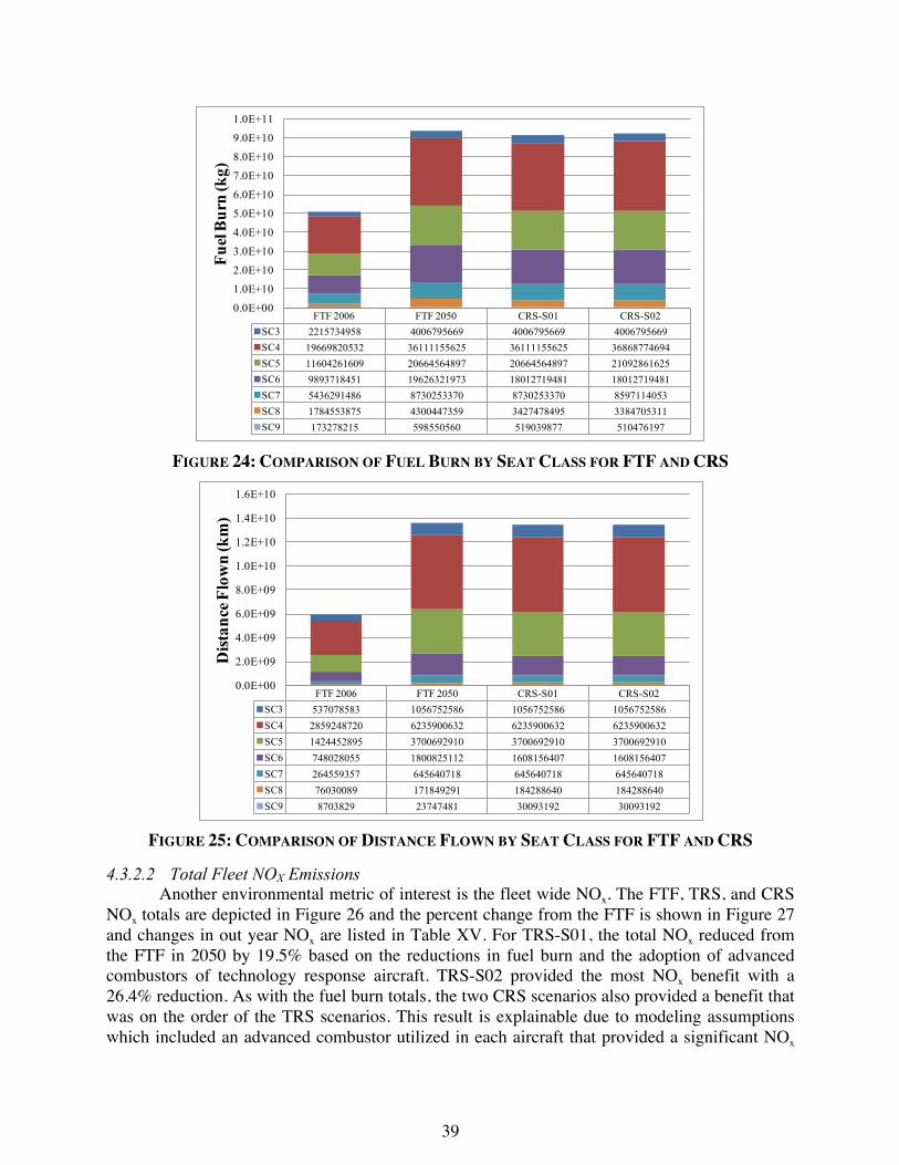
39

FTF 2006 FTF 2050 CRS-S01 CRS-S02SC3 2215734958 4006795669 4006795669 4006795669SC4 19669820532 36111155625 36111155625 36868774694SC5 11604261609 20664564897 20664564897 21092861625SC6 9893718451 19626321973 18012719481 18012719481SC7 5436291486 8730253370 8730253370 8597114053SC8 1784553875 4300447359 3427478495 3384705311SC9 173278215 598550560 519039877 510476197

0.0E+00

1.0E+10

2.0E+10

3.0E+10

4.0E+10

5.0E+10

6.0E+10

7.0E+10

8.0E+10

9.0E+10

1.0E+11

Fuel

Bur

n (k

g)

FIGURE 24: COMPARISON OF FUEL BURN BY SEAT CLASS FOR FTF AND CRS

FTF 2006 FTF 2050 CRS-S01 CRS-S02SC3 537078583 1056752586 1056752586 1056752586SC4 2859248720 6235900632 6235900632 6235900632SC5 1424452895 3700692910 3700692910 3700692910SC6 748028055 1800825112 1608156407 1608156407SC7 264559357 645640718 645640718 645640718SC8 76030089 171849291 184288640 184288640SC9 8703829 23747481 30093192 30093192

0.0E+00

2.0E+09

4.0E+09

6.0E+09

8.0E+09

1.0E+10

1.2E+10

1.4E+10

1.6E+10

Dist

ance

Flo

wn

(km

)

FIGURE 25: COMPARISON OF DISTANCE FLOWN BY SEAT CLASS FOR FTF AND CRS

4.3.2.2 Total Fleet NOX Emissions Another environmental metric of interest is the fleet wide NOx. The FTF, TRS, and CRS

NOx totals are depicted in Figure 26 and the percent change from the FTF is shown in Figure 27 and changes in out year NOx are listed in Table XV. For TRS-S01, the total NOx reduced from the FTF in 2050 by 19.5% based on the reductions in fuel burn and the adoption of advanced combustors of technology response aircraft. TRS-S02 provided the most NOx benefit with a 26.4% reduction. As with the fuel burn totals, the two CRS scenarios also provided a benefit that was on the order of the TRS scenarios. This result is explainable due to modeling assumptions which included an advanced combustor utilized in each aircraft that provided a significant NOx

40

reduction from the baseline aircraft. Had the combustors not been added, the benefits to NOx would have been on the order of the fleet fuel burn saving of a few percent. The major seat class drivers were SC6 which had approximately a 40% reduction over the baseline aircraft and in SC8/9 which was approximately 70%. These benefits are completely driven by the performance and the addition of the advanced combustors of the response vehicles.

600

700

800

900

1,000

1,100

1,200

1,300

2005 2010 2015 2020 2025 2030 2035 2040 2045 2050

Flee

t Miss

ion

NO

x (g

)B

illio

ns

Year

Baseline FTF TRS-S01 TRS-S02 CRS-S01 CRS-S02

FIGURE 26: TOTAL FLEET NOX EMISSIONS

-30%

-25%

-20%

-15%

-10%

-5%

0%2015 2020 2025 2030 2035 2040 2045 2050

% C

hang

e fro

m B

asel

ine F

leet

NO

x To

tal

Year

TRS-S01 TRS-S02 TRS-S01 TRS-S02

FIGURE 27: NOX % CHANGE FROM BASELINE

41

TABLE XV: FLEET NOX TOTALS BY INCREMENTAL OUT-YEARS Scenario 2006 2010 2020 2030 2040 2050 FTF (g) 7.3224E+11 6.6817E+11 7.9774E+11 9.2253E+11 1.0910E+12 1.2852E+12

TRS-S01 0.00% 0.00% -1.40% -11.43% -17.15% -19.54% TRS-S02 0.00% 0.00% -2.30% -16.1% -23.43% -26.42% CRS-S01 0.00% 0.00% -1.42% -8.95% -12.07% -13.39% CRS-S02 0.00% 0.00% -1.42% -12.03% -18.20% -20.87%

4.3.2.3 Fleet Noise Exposure The last environmental metric considered was the impact to DNL at two notional airports

resulting from the baseline FTF, TRS, and CRS scenarios. Noise contour areas were calculated using ANGIM for one-runway and four-runway airports in 2050 for all scenarios, and were compared to baseline contours calculated in 2050; the one-runway is a regional airport and the four-runway is a large hub. Contour area in 2050 was investigated to determine noise impacts in the long-term, and GREAT was used to provide flight schedules at each airport in 2006 and 2050 to ensure consistency with the rest of the fleet-level metrics. As explained previously, ANGIM calculates contour areas by accumulating individual aircraft grids, and noise grids for each aircraft identified in the GREAT schedules had to be obtained. Noise grids for EDS Generic Vehicles and all technology and capability response vehicles were provided by EDS, through the use of Georgia Tech's custom AEDT "Tester" which leverages core AEDT functionality to compute noise [24].

Although, at the time of this study, EDS Generic Vehicles were developed to represent average performance for fuel burn and NOx and not explicitly for noise, their use for fleet-wide noise analysis was still desired because of their resulting noise performance, which was still a very reasonable average of vehicles in each class. Furthermore, and more importantly, the impacts of any potential deficiencies or inaccuracies in the EDS Generic Vehicle model with respect to noise were minimized by using consistent assumptions across scenarios and drawing observations only across scenarios in a given year. The use of consistent operations, replacement, and runway assignment assumptions across scenarios at each airport meant that the use of EDS Generic Vehicles was legitimate for providing very valuable insight into the trends related to the introduction of technology or capability response vehicles on flee level noise. This study therefore focused analysis and observations on changes in airport contour area not between out years, but rather between scenarios at the same airport in a specific year compared to the baseline, where aircraft-specific impacts were isolated.

Noise grids for all other existing aircraft also leveraged the AEDT "Tester," but relied upon existing AEDT characterizations for their performance. The operations schedules provided by GREAT for each airport detailed specific operation counts for each aircraft by stage length and time of day to enable accurate calculate of DNL. Although ANGIM is capable of calculating contour areas for any noise level, levels near 65 dB DNL were reported since this compares best to typical metrics used for noise exposure [25]. Airport configuration assumptions for each airport were also required, including number, orientation, and traffic assignment of runways.

Using the operations results from GREAT for all metric systems and scenarios, the impacts to YDNL at two notional airports were then analyzed. Results were first generated for the FTF case, since this was the baseline against which other scenarios were compared. The FTF case was investigated in 2006 and in 2050 to determine the general change in noise exposure in

42

the absence of any new notional standards. The change in contour area from 2006 to 2050 for several DNL levels at both airports for the FTF case is listed in Table XVI. In this FTF case, the large increase in contour area for all levels is due almost entirely to the forecasted increase in operations in 2050; a small degree of change in fleet mix, due to the retirement of old technology and replacement by 2006 technology levels, makes the average fleet-wide noise performance slightly better in 2050 than in 2006, but is dominated by operation volume affecting cumulative contour areas. A depiction of the resulting contours in 2006 and 2050 from 60-75 dB DNL is given for both airports in Figure 28.

TABLE XVI: NOISE CONTOUR CHANGES BETWEEN 2006 BASELINE AND 2050 FTF

Contour Level

(YDNL dB)

1-Runway Airport 4-Runway Airport S00 2050

(% from 2006) S00 2050

(% from 2006) 60 129.08 118.42 65 117.03 97.33 70 143.96 93.00 75 186.02 128.17

FIGURE 28: ONE- AND FOUR-RUNWAY AIRPORT CONTOURS IN 2006 AND 2050

The percent change of the 2050 TRS-S01, TRS-S02, CRS-S01, and CRS-S02 scenarios with respect to the 2050 FTF results for the one-runway airport are listed in Table XVII. One observation for this analysis is the reduction in contour area for both TRS scenarios, by a minor amount in the conservative S01 and by as much as -17% in the more aggressive S02. Since the TRS scenarios incorporated only technology addition in comparison to the FTF case, the observed behavior is due solely to the introduction of favorable technology to reduce the size of the aircraft. Although technologies introduced were aimed for fuel efficiency improvements, the simultaneous reduction in noise suggests the interdependencies associated with this metric system favorably provide benefits for multiple environmental metrics.

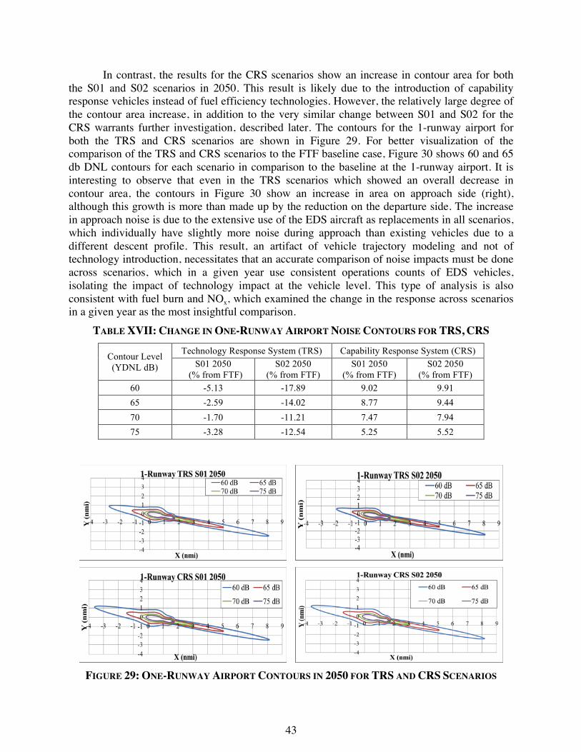
43

In contrast, the results for the CRS scenarios show an increase in contour area for both the S01 and S02 scenarios in 2050. This result is likely due to the introduction of capability response vehicles instead of fuel efficiency technologies. However, the relatively large degree of the contour area increase, in addition to the very similar change between S01 and S02 for the CRS warrants further investigation, described later. The contours for the 1-runway airport for both the TRS and CRS scenarios are shown in Figure 29. For better visualization of the comparison of the TRS and CRS scenarios to the FTF baseline case, Figure 30 shows 60 and 65 db DNL contours for each scenario in comparison to the baseline at the 1-runway airport. It is interesting to observe that even in the TRS scenarios which showed an overall decrease in contour area, the contours in Figure 30 show an increase in area on approach side (right), although this growth is more than made up by the reduction on the departure side. The increase in approach noise is due to the extensive use of the EDS aircraft as replacements in all scenarios, which individually have slightly more noise during approach than existing vehicles due to a different descent profile. This result, an artifact of vehicle trajectory modeling and not of technology introduction, necessitates that an accurate comparison of noise impacts must be done across scenarios, which in a given year use consistent operations counts of EDS vehicles, isolating the impact of technology impact at the vehicle level. This type of analysis is also consistent with fuel burn and NOx, which examined the change in the response across scenarios in a given year as the most insightful comparison.

TABLE XVII: CHANGE IN ONE-RUNWAY AIRPORT NOISE CONTOURS FOR TRS, CRS

Contour Level (YDNL dB)

Technology Response System (TRS) Capability Response System (CRS) S01 2050

(% from FTF) S02 2050

(% from FTF) S01 2050

(% from FTF) S02 2050

(% from FTF) 60 -5.13 -17.89 9.02 9.91 65 -2.59 -14.02 8.77 9.44 70 -1.70 -11.21 7.47 7.94 75 -3.28 -12.54 5.25 5.52

FIGURE 29: ONE-RUNWAY AIRPORT CONTOURS IN 2050 FOR TRS AND CRS SCENARIOS

44

FIGURE 30: ONE-RUNWAY AIRPORT TRS AND CRS CONTOUR COMPARISON TO FTF

The noise impacts of the TRS and CRS scenarios were also analyzed for a large hub, four-runway airport, to give insight into the potential behavior of noise trends across a variety of airports in the NAS. The change in contour area in 2050 relative to the FTF case is listed for the TRS and CRS scenarios in Table XVIII. The impacts to contour area were observed to be very similar to the one-runway airport; the TRS showed minor reduction in area in S01 and a larger reduction in S02, while the CRS showed similar increases in area in both scenarios. It is interesting to note that the degree of improvement in S01 for the TRS was slightly less in the four-runway airport than in the one-runway airport, likely due either to the specific fleet mix at this airport which may not be as highly impacted by technology addition as other airports, or simply the shape of this airport's contour, which may be less sensitive due to its configuration.

The 2050 contours for several noise levels are given for the four-runway airport in Figure 31 for both the TRS and CRS scenarios. Once again, it is observed that the contour shape was highly driven by the airport configuration and runway layout; higher dB DNL show pockets of isolated behavior very near two sets of parallel runways, individually clustered near the top and bottom, while lower DNL had much broader shape that encompasses the entire airport. Also, it is observed that the contours were heavily impacted by operations on the departure end (left), which generally produce more noise than approach. Finally, a comparison of 60-65 dB DNL contours between the baseline FTF case and the TRS and CRS scenarios is given in Figure 32 An interesting observation for the TRS scenarios is that similar to the one-runway airport, from Figure 32 it is noticeable that the contours on the approach side (right) of the four-runway airport also grew in comparison to the FTF case, although this was more than made up by the decrease in area on the departure side. This result was also driven by the differing descent trajectory of EDS aircraft compared to existing aircraft, and not due to technology introduction.

45

TABLE XVIII: CHANGE IN FOUR-RUNWAY AIRPORT NOISE CONTOURS FOR TRS, CRS Contour

Level (YDNL dB)

Technology Response System (TRS) Capability Response System (CRS) S01 2050

(% from FTF) S02 2050

(% from FTF) S01 2050

(% from FTF) S02 2050

(% from FTF) 60 -2.29 -13.03 9.51 9.78 65 -2.04 -11.54 11.49 12.14 70 -0.64 -8.02 9.53 9.93 75 -3.39 -11.83 7.55 7.78

Considering the behavior of the noise response of the CRS scenarios, a closer look was

required to explain the unexpected increase in noise contour area relative to the FTF baseline. As a first step, the operations per aircraft seat class were investigated at both airports to determine which particular aircraft classes may be dominating the noise response. Using the operations counts provided by GREAT, the percentages of total operations at the one- and four-runway airports broken down by aircraft seat class are depicted in Figure 33. It is observed that the operations were dominated by seat class 4 at both airports, which corresponded to SA aircraft. The next biggest contributor to total operations at both airports is seat class 5, which was also the SA class. Seat class 6, corresponding to small twin-aisle aircraft was the next largest contributor at the 1-runway airport, and also significant at the 4-runway airport, while seat class 3, or regional jet aircraft was the third-largest contributor at the 4-runway airport. This behavior was generally consistent with the total operations split observed in GREAT, shown previously.

FIGURE 31: FOUR-RUNWAY AIRPORT CONTOURS IN 2050 FOR TRS AND CRS SCENARIOS

46

FIGURE 32: FOUR-RUNWAY AIRPORT TRS AND CRS CONTOUR COMPARISON TO FTF

4-­‐Runway  Airport  2050  Operations

SC3

SC4

SC5

SC6

SC7

SC8

SC9

1-­‐Runway  Airport  2050  Operations

SC3

SC4

SC5

SC6

SC7

SC8

SC9

FIGURE 33: 2050 OPERATIONS SPLIT AT ONE- AND FOUR-RUNWAY AIRPORTS

Although aircraft with the most operations do not always account for the most noise, the operations split shown in Figure 33 can help explain the TRS and CRS noise results shown previously. Since the SA class dominated total operations, the noise characteristics of this aircraft class should be considered. First, it was noteworthy that in the TRS, the SA class used either baseline or in-production technology replacements, while the CRS only used baseline variants, as listed in Table XI and Table XII, respectively. This behavior suggests that different noise characteristics were expected for the TRS and CRS for this aircraft class, given the different aircraft used. Different behavior was indeed observed when examining the single event noise contours of the single aisle class aircraft, shown in Figure 34. Here, it is observed that the baseline variants used in the CRS had nearly identical noise characteristics, while the in-production technology variants used in the TRS had significantly smaller noise footprint, primarily due to a re-engine. The much smaller noise footprint for this aircraft class in the TRS helped explain the expected result of a decrease in contour area for the TRS in S01 and S02. A similar result was observed for approach.

47

-3

-2

-1

0

1

2

3

-2 0 2 4 6 8 10 12 14 16Y (n

mi)

X (nmi)

SC4/5

150pax: Baseline, FTF. TRS-S01 (2017), CRS-S01, CRS-S02 (2017)In Prod. Tech: TRS-S01 (2023), TRS-S02

HB Base Fuselage: CRS-S02 (2023)

FIGURE 34: SINGLE-EVENT NOISE CONTOURS FOR SINGLE AISLE CLASS AIRCRAFT

The nearly identical behavior of the baseline variants in the CRS, however, did not explain the overall growth in contour area in CRS scenarios S01 and S02. The contribution to noise of the regional jet class, or SC3, also did not explain the CRS behavior because this aircraft, like the single aisle, also used baseline aircraft in S01 and S02, and thus did not account for the increase in noise. The increase in contour area for the CRS, then, was due to SC6, or the small twin-aisle aircraft class, the only other significant contributor to operations at either airport. The single-event noise contours for this class aircraft, and its replacements used in the TRS and CRS scenarios are shown in Figure 35. In the TRS, technology-infused small twin-aisle aircraft were used as replacements, yielding a reduction in contour area of approximately 20%. In the CRS, the nature of the metric system which enabled aircraft of different capability to meet fuel efficiency stringency resulted in the use of larger aircraft as replacements for this seat class, resulting in more noise than the baseline. Figure 35 shows that the LTA LL, used as replacements for STA aircraft in the CRS, resulted in a noise footprint approximately 12% larger than the baseline for each operation. Given the contribution of this class aircraft to operations at both airports, the increased noise of this seat class helped explain why the CRS resulted in increased contour area for S01 and S02. A similar behavior was observed for the LTA class in the CRS, although it accounted for an insignificant contribution to operations at either airport.

-3

-2

-1

0

1

2

3

-2 0 2 4 6 8 10 12 14 16Y (n

mi)

X (nmi)

SC6

210pax: Baseline, FTF

In Prod. Tech: TRS-S01, TRS-S02

LTA LL: CRS-S01, CRS-S02

FIGURE 35: SINGLE-EVENT NOISE CONTOURS FOR SC6 AIRCRAFT

The unexpected increase in noise exposure of the CRS in this research was concerning, although its explanation yields an important finding of this research: the use of a capability response system for a fuel efficiency standard may result in unintended consequences at the system level, and can lead to detrimental impacts to other environmental impacts. This important finding can help inform the consideration of the most appropriate metric system for the development of a fuel efficiency standard and its impacts to the NAS.

48

4.3.3 APMT-Impacts Climate Results In order to calculate the climate environmental benefits due to the scenarios proposed in

Table II, the APMT-Impacts climate module was used. Together the three APMT-Impacts modules, Noise, Air Quality, and Climate, assess the physical and socio-economic environmental impacts of aviation using noise and emissions inventories as the primary inputs. Impacts and associated uncertainties are simulated based on a probabilistic approach using Monte Carlo methods. The climate module was the only module used for the analysis presented here.

The APMT-Impacts Climate Module estimates CO2 and non-CO2 impacts using both physical and monetary metrics [26,27,28,29]. The temporal resolution of the APMT Climate Module is one year while the spatial resolution is at a highly aggregated global mean level. The effects modeled include long-lived CO2, and short-lived non-CO2 effects including the short-lived impact of NOX on ozone (NOX-O3 short), the production of cirrus, sulfates, soot, H2O, and contrails. Also included are the NOX-CH4 interaction and the associated primary mode NOX-O3 effect (referred to as NOX-O3 long).

Aircraft emissions are treated as pulse emissions emitted each year during a scenario, ultimately leading to changes in globally-averaged surface temperature. Pulses of aircraft CO2 and NOX emissions lead to direct and indirect radiative forcing effects. Aircraft fuel burn is used as a surrogate for other short-lived climate effects such as contrails, induced cirrus cloudiness, water vapor, soot, and sulfates. Longer-lived radiative forcing impacts associated with yearly pulses of CO2 and NOX emissions decay according to their e-folding times, while the RF from short-lived effects including the warming NOX-O3 effect is assumed to last only during the year of emissions. A superposition of decaying pulses or a convolution of the perturbation with the impulse response function of the system provides the temporal variation in the different effects modeled. The code description presented here, and a detailed description of the APMT Climate Module are published in Mahashabde A, et al. [30].

When conducting an analysis using the climate code, lenses are used to represent a range of inputs and code parameters. The climate code has a set of parameters that are depicted using an uncertainty distribution or where a discreet choice for the value of that parameter exists. One can conceive of thousands of unique combinations of inputs and model parameters that may be of interest in assessing different policy options. In order to extract meaningful insights about the possible costs and benefits of a policy, it is therefore necessary for the analysis options to be synthesized into a set of pre-defined combinations of inputs and assumptions. These combinations of inputs and model parameters can be thought of as describing a particular point of view or perspective and are thus designated as lenses. The climate code is typically run using a low, mid, and high lens to represent the best, mid, and worst case scenario of impacts. The lens settings used in this analysis are shown in Table XIX. Further, given the non-deterministic nature of the code and lens distributions, Monte Carlo simulations were run to provide a statistically significant sample. Finally, a range of discount rates was analyzed to provide a sensitivity analysis for policy makers considering different levels of risk. A summary of the input settings for the climate model is given below and described in more detail in Table XIX.

§ 10,000 Monte Carlo Simulations

49

§ Policy start date: 2018 § Policy years of input data: 2010, 2020, 2030, 2040, 2050 § Impacts calculated for 800 years from policy end date (2050) § Discount rate: 2%, 3%, 7% § Lenses as specified in Table XIX

TABLE XIX: APMT-IMPACTS CLIMATE CODE LENS SETTINGS

Climate Assumptions Low Lens (Best Case / Low Impact)

Mid Lens High Lens (Worst Case / Conservative)

Climate Sensitivity 2 K Triangular distribution [3, 2-4.5] K

4.5 K

NOX – related effects Stevenson et al. (2004) Discrete Uniform distribution Wild et al. (2001). Short-lived effects relative RF [AIC, Sulfates, Soot,

H2O, contrails]

[11, -29.3, 0.56, 0.39, 5.4] mW/m2

Triangular distribution [(11,33,87), (-29.3, -4.8,

.79), (.56, 3.4, 20.7), (0.39, 2.8 20.3), (5.4, 11.8, 25.6)]

mW/m2

[87, -0.79, 20.7, 20.3, 25.6] mW/m2

Background Scenario A2 B2 A1B Damage Coefficient 5th Percentile DICE Normal Distribution

DICE-2007 95th Percentile DICE

Mixed Layer Heat Capacity

2.53e8 J/(K * m2) Triangular Distribution [4.41, 2.53-6.31] 108 J/(K *

m2)

6.31e8 J/(K * m2)

Advective Flux 2.46e-4 kg/(m2 * s) Triangular Distribution [1.23, 2.46-0.62] 10-4 kg/(m2

* s)

6.2e-5 kg/(m2 * s)

Diffusion 1e-4 m2/s Uniform Distribution 4.4-10 10-5 m2/s

4.4e-5 m2/s

Deep Ocean Heat Capacity

2.52e10 J/(K * m2) Triangular Distribution [1.26, 6.39-25.2] 109 J/(K * m2)

6.3e9 J/(K * m2)

Mixing Depth 500 m Triangular Distribution [1000, 500-2000] m

2000 m

The results of the APMT-Impacts climate analysis are shown below. Figure 36 through

Figure 38 show the physical damages, or the change in temperature that is expected as a result of the policy. Figure 39 and Figure 40 show the Net Present Value (NPV) of implementing each policy. It should be noted that the results presented here are based on theoretical scenarios that may be revised in future work. Figure 36 shows the impact of the baseline on global average temperature, with the shaded area representing the total impact. The impact is broken down by emission species and both warming and cooling effects are present. It can be seen that CO2 emissions have a long lasting effect, while the other impacts fade by 2100. Figure 37 shows the total impact on temperature for the baseline and each scenario under consideration. Figure 38 shows the impact on temperature for policy minus baseline. It can be seen that in all cases the policy results in a decrease in temperature, while the technology-only scenarios (TRS-S01 and TRS-S02) have a greater reduction in temperature when compared with the transport-capability-only scenarios (CRS-S01 and CRS-S02).

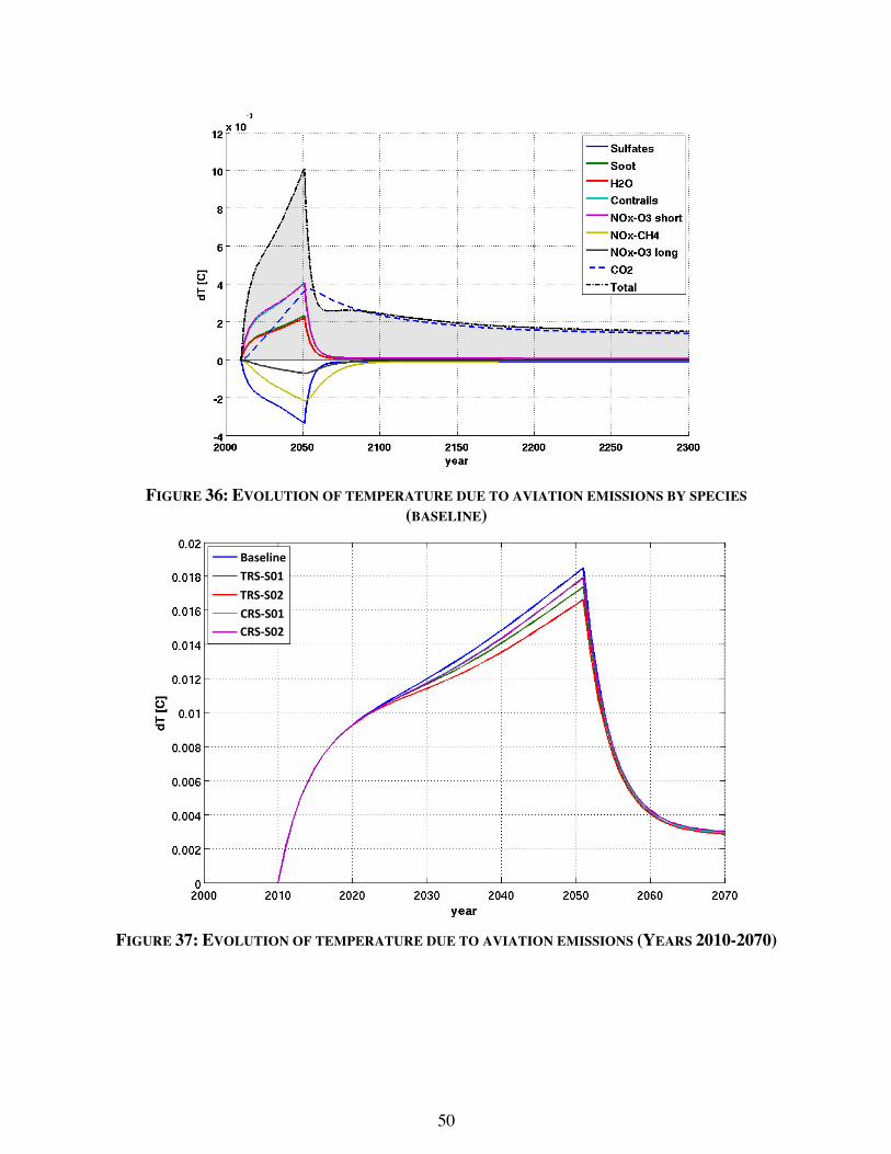
50

FIGURE 36: EVOLUTION OF TEMPERATURE DUE TO AVIATION EMISSIONS BY SPECIES

(BASELINE)

!"#$#%&'

!"#$#%(')"#$#%&')"#$#%('

*+,-./0-'

FIGURE 37: EVOLUTION OF TEMPERATURE DUE TO AVIATION EMISSIONS (YEARS 2010-2070)

51

!"#$#%&'

("#$#%&'("#$#%)'

!"#$#%)'

FIGURE 38: EVOLUTION OF TEMPERATURE DUE TO AVIATION EMISSIONS (∆T FROM BASELINE)

Figure 39 and Figure 40 show the delta NPV (policy minus baseline) for all of the scenarios being considered. NPV is calculated by computing the value of the reduced damages incurred due to less emissions expelled into the environment. In all cases monetary savings in terms of present value can be expected as a result of the policy implementation, with greater savings apparent for the technology-only scenarios. However, significant variation in the magnitude of the benefit is observed when lens assumptions and discount rates are varied.

!"

#!"

$!"

%!"

&!"

'!"

(!"

)!"

!"#

$%&'$())*+$

!"#$,-$./012,3$4151678$9:!"#$-;,5$'187<037=$$

*+,"*-./"

012"*-./"

3145"*-./"

!

!"#$

!%#$

!&#$

!'#$

!(#$

!)#$

!*#$

#$

!"#

$%&'$())*+$

!"#$,-$./012,3$4151678$9:!"#$-;,5$'187<037=$$

+,-$+./0$

123$+./0$

4256$+./0$

!"#$ !"%$ !"&$ !"'$

()**+*$,-*.$/01/2-34$#"35$-01$6"35$74*240894$:-9;4.<$

!!"#$#%&'''' !"#$#%(' )"#$#%&' )"#$#%(' FIGURE 39: ∆NPV (POLICY – BASELINE); SENSITIVITY TO BACKGROUND LENS ASSUMPTION

52

!"

#"

$!"

$#"

%!"

%#"

&!"

&#"

!"#

$%&'$())*+$

!"#$,-$./012,3$4151678$9:!"#$-;,5$'187<037=$$

'()%*"

'()&*"

'()+*"

!"#$

!"%$

!&#$

!&%$

!'#$

!'%$

!#$

%$

!"#

$%&'$())*+$

!"#$,-$./012,3$4151678$9:!"#$-;,5$'187<037=$$

()*&+$

()*"+$

()*,+$

!"#$ !"%$ !"&$ !"'$

()**+*$,-*.$/01/2-34$#"35$-01$6"35$74*240894$:-9;4.<$

!!"#$#%&' !"#$#%(' )"#$#%&' )"#$#%(' FIGURE 40: ∆NPV (POLICY - BASELINE); SENSITIVITY TO DISCOUNT RATE (DR)

5 Conclusions

This report investigated the implications of two possible response scenarios resulting from a CO2 certification standard for future aircraft. This research expanded upon previous, related work in this area by examining potential responses and additional environmental impacts. The analyses described in this report detail the systematic analyses undertaken to quantify potential NAS level environmental impacts of different types of response scenarios, and the associated assumptions under which the observations are valid. The findings and observations included in this research are intended to provide insight into the potential implications of response scenarios on the NAS, and support the decision-making processes for mitigating the environmental impacts of aircraft operations within the NAS.

In this research, two response scenarios were identified based on assumed potential responses from metric systems exhibiting TCN and non-TCN characteristics. The TCN metric system was assumed to be sensitive only to technology introduction, thus a technology response system (TRS), while the non-TCN metric system was assumed to be sensitive only to aircraft capability, and was thus a capability response system (CRS). Baseline fleet trends were determined for both metric systems, which were then used to develop moderate and aggressive scenarios to represent limits for analysis. Responses to each scenario were developed to enable aircraft to meet the moderate and aggressive limits and leveraged new and in-production EDS technology roadmaps as well as various constant technology EDS aircraft representing different payload and range transport capabilities. Responses for the TRS involved only technology packages, while responses for the CRS included transport capability variants. Responses to each metric system were used as replacement vehicles in a fleet analysis, and used in conjunction with demand forecast and other assumptions to quantify the resulting system totals for fuel consumption and NOx until 2050, and noise contour area at two airports in 2050. The fleet results in 2050 were then analyzed by APMT for further insight into the environmental impacts.

This research found that the TRS had a greater benefit on the NAS in terms of fuel consumption, NOx emissions, noise contour area, and climate impacts than the CRS. The aggressive limit scenario for the TRS produced 9.5% reduction in fuel consumption, 26%

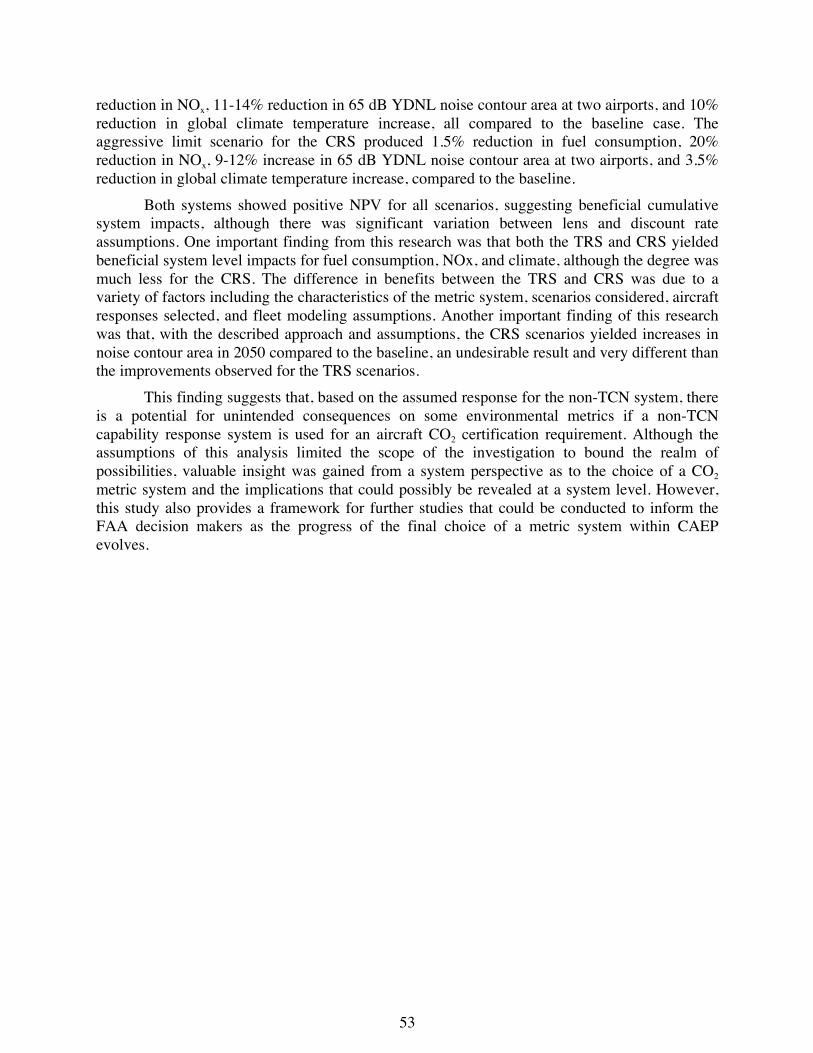
53

reduction in NOx, 11-14% reduction in 65 dB YDNL noise contour area at two airports, and 10% reduction in global climate temperature increase, all compared to the baseline case. The aggressive limit scenario for the CRS produced 1.5% reduction in fuel consumption, 20% reduction in NOx, 9-12% increase in 65 dB YDNL noise contour area at two airports, and 3.5% reduction in global climate temperature increase, compared to the baseline.

Both systems showed positive NPV for all scenarios, suggesting beneficial cumulative system impacts, although there was significant variation between lens and discount rate assumptions. One important finding from this research was that both the TRS and CRS yielded beneficial system level impacts for fuel consumption, NOx, and climate, although the degree was much less for the CRS. The difference in benefits between the TRS and CRS was due to a variety of factors including the characteristics of the metric system, scenarios considered, aircraft responses selected, and fleet modeling assumptions. Another important finding of this research was that, with the described approach and assumptions, the CRS scenarios yielded increases in noise contour area in 2050 compared to the baseline, an undesirable result and very different than the improvements observed for the TRS scenarios.

This finding suggests that, based on the assumed response for the non-TCN system, there is a potential for unintended consequences on some environmental metrics if a non-TCN capability response system is used for an aircraft CO2 certification requirement. Although the assumptions of this analysis limited the scope of the investigation to bound the realm of possibilities, valuable insight was gained from a system perspective as to the choice of a CO2 metric system and the implications that could possibly be revealed at a system level. However, this study also provides a framework for further studies that could be conducted to inform the FAA decision makers as the progress of the final choice of a metric system within CAEP evolves.

54

6 Appendix A

6.1 Technology Portfolio for Policy Scenario Considerations TABLE XX: SUMMARY OF AVAILABLE FUEL BURN TECHNOLOGIES

Technology Description Assumed Impacts Airframe - Structure

Retro-Fit Winglet and planar wing tips

Winglets are applied to the edges of the wing and effectively reduce the induced drag of the aircraft

-Reduce induced drag -Increase wing weight

Retro-Fit Alternate non-planar wing tips

Winglets are applied to the edges of the wing and effectively reduce the induced drag of the aircraft

-Reduce induced drag -Increase wing weight

Metallic Technologies Aircraft manufacturing techniques such as laser beam welding and electron beam welding can reduce weight of the aircraft

-Reduced aircraft structural weight

Composite Technologies Composite materials are lighter than their conventional metal counterparts and are used in the aircraft fuselage, wing, and horizontal and vertical tails to reduce weight

-Reduced aircraft structural weight

Structural Health Monitoring (SHM)

Structural health monitoring allows aircraft to be designed closer to the critical limits of materials. This allows components to be designed with a lower factor of safety which reduces weight

-Reduced aircraft structural weight

Nanotechnologies Nanotechnologies could potentially be used to create integrated circuits that reduce weight.

-Reduced aircraft structural weight

Multifunctional Structures This is a wide category of technologies and includes self healing technologies that can reduce the weight of the aircraft since parts can be designed closer to their limits

-Reduced aircraft structural weight

Airframe - Aerodynamic Adaptive Wing/Variable Camber

A variable camber trailing edge system allows for the camber of the wing to change during flight to optimize aerodynamic efficiency

-Increased wing weight -Reduced aircraft drag

Shock Bumps Shock bumps reduce the wave drag over the wing in off design conditions

-Reduced aircraft drag

Morphing Wing Uses smart materials to change the shape of the airfoil during flight, such as the upper surface.

-Increased wing weight -Reduced aircraft drag

Natural Laminar Flow Control (NLF)

Airfoils are designed such that the laminar to turbulent transition of the boundary layer is delayed, thereby reducing drag

-Reduced wing profile drag

Hybrid Laminar Flow Control (HLFC)

Suction is used to control the boundary layer over the airfoil and maintain a laminar boundary layer

-Reduced profile drag -Increased wing weight due to ducting -Increased power requirements on engine due to suction

Discrete Roughness Elements

Small roughness elements are placed on the wing to delay boundary layer transition to

-Minor increase in wing weight

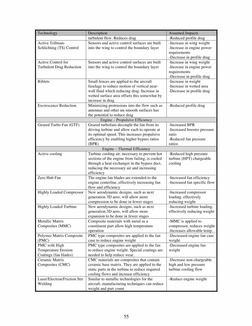
55

Technology Description Assumed Impacts turbulent flow. Reduces drag -Reduced profile drag

Active Tollman-Schlichting (TS) Control

Sensors and active control surfaces are built into the wing to control the boundary layer

-Increase in wing weight -Increase in engine power requirements -Decrease in profile drag

Active Control for Turbulent Drag Reduction

Sensors and active control surfaces are built into the wing to control the boundary layer

-Increase in wing weight -Increase in engine power requirements -Decrease in profile drag

Riblets Small fences are applied to the aircraft fuselage to reduce motion of vertical near-wall fluid which reducing drag. Increase in wetted surface area offsets this somewhat by increase in drag

-Increase in weight -Increase in wetted area -Decrease in profile drag

Excrescence Reduction Minimizing protrusions into the flow such as antennas and other un-smooth surfaces has the potential to reduce drag

-Reduced profile drag

Engine – Propulsive Efficiency Geared Turbo Fan (GTF) Geared turbofans decouple the fan from its

driving turbine and allow each to operate at its optimal speed. This increases propulsive efficiency by enabling higher bypass ratios (BPR)

-Increased BPR -Increased booster pressure ratio -Reduced fan pressure ratios

Engine – Thermal Efficiency Active cooling Turbine cooling air, necessary to prevent hot

sections of the engine from failing, is cooled through a heat exchanger in the bypass duct, reducing the necessary air and increasing efficiency

-Reduced high pressure turbine (HPT) chargeable cooling

Zero Hub Fan The engine fan blades are extended to the engine centerline, effectively increasing fan flow and efficiency

-Increased fan efficiency -Increased fan specific flow

Highly Loaded Compressor New aerodynamic designs, such as next generation 3D aero, will allow more compression to be done in fewer stages

-Increased compressor loading, effectively reducing weight

Highly Loaded Turbine New aerodynamic designs, such as next generation 3D aero, will allow more expansion to be done in fewer stages

-Increased turbine loading, effectively reducing weight

Metallic Matrix Composites (MMC)

Composite materials with metal as a constituent part allow high temperature operation

-MMC is applied to compressor, reduces weight -Increases allowable temp.

Polymer Matrix Composite (PMC)

PMC type composites are applied to the fan case to reduce engine weight

-Decreased engine fan case weight

PMC with High Temperature Erosion Coatings (fan blades)

PMC type composites are applied to the fan to reduce engine weight. Special coatings are needed to help reduce wear.

-Decreased engine fan weight

Ceramic Matrix Composites (CMC)

CMC materials are composites that contain ceramic base matrix. They are applied to the static parts in the turbine to reduce required cooling flows and increase efficiency

-Decrease non-chargeable high and low pressure turbine cooling flow

Laser/Electron/Friction Stir Welding

Similar to metallic technologies for the aircraft, manufacturing techniques can reduce weight and part count.

-Reduce engine weight

56

Technology Description Assumed Impacts Turbine Active Clearance Control

-Next generation active clearance control systems will enable tighter engine tolerances and increase component efficiency

-Increase turbine efficiency -Increase turbine weight

Compressor Active Clearance Control

-Next generation active clearance control systems will enable tighter engine tolerances and increase component efficiency

-Increase compressor efficiency -Increase compressor weight

Advanced Turbine Disk Alloys

Next generation alloys will enable hotter operational temperatures, reducing required cooling flows

-Reduce required cooling in HPT and LPT

Advanced TBC (on blades only)

Thermal barrier coatings insulate hot sections of the engine from hot gasses and reduce cooling flows

-Reduce required chargeable cooling in HPT and LPT

HPC Flow Control Similar to hybrid laminar flow control on an aircraft, flow control can be used to increase engine component efficiency

-Increased component efficiency -Air source penalty for flow control

Turbine Flow Control

TABLE XXI: SUMMARY OF AVAILABLE PRODUCTION-LINE FUEL BURN TECHNOLOGIES

Technology Description Assumed Impacts Technologies Available for Production Line Application

Excrescence Reduction Minimizing protrusions into the flow such as antennas and other un-smooth surfaces has the potential to reduce drag

- Reduced profile drag

Riblets Small fences are applied to the aircraft fuselage to reduce motion of vertical near-wall fluid which reducing drag. Increase in wetted surface area offsets this somewhat by increase in drag

- Increase in weight - Increase in wetted area - Decrease in profile drag

Lighter cabin furnishing Use of modern seats weighing 30-40% less than predecessors, and cabin carpeting 0.68lbs/square-yard lighter

- Decreased furnishings weight

Drooped aileron Reconfiguration of flight control software to droop aileron 2o, modifying span-wise lift distribution and decreasing drag

- Reduce induced drag - Slightly increases profile drag

Resized vortex generators Redesigned vortex generators along wing that reduce drag

- Reduced profile drag

Engine performance improvement package

Improved aerodynamic efficiency of turbomachinery to reduce TSFC

- Increased component efficiency throughout

Re-engine New thermodynamic cycle selected to loosely predict next-generation of engine in each class

- Advanced cycle technology throughout

57

Technologies TRL Time to TRL =9

TRL9 Date 20

10

2011

2012

2013

2014

2015

2016

2017

2018

2019

2020

2021

2022

2023

2024

2025

2026

2027

2028

2029

2030

Retro-Fit Winglet and planar wing tips 9 0 2010 9Retro-Fit Alternate non-planar wing tips 4 14 2024 9 9 9 9 9 9 9 9 9 9 9 9 9 9 9Metallic Technologies 9 0 2010 9Composite Technologies 9 0 2010 9Structural Health Monitoring 2 15.5 2026 9 9 9 9 9 9 9 9 9 9 9 9 9 9 9 9 9Nanotechnologies 2 15.5 2026 9 9 9 9 9 9 9 9 9 9 9 9 9 9 9 9 9Multifunctional Structures 3 14.8 2025 9 9 9 9 9 9 9 9 9 9 9 9 9 9 9 9Adaptive Wing/Variable Camber 4 14 2024 9 9 9 9 9 9 9 9 9 9 9 9 9 9 9Shock Bumps 3 14.8 2025 9 9 9 9 9 9 9 9 9 9 9 9 9 9 9 9Morphing Wing 2 15.5 2026 9 9 9 9 9 9 9 9 9 9 9 9 9 9 9 9 9Natural Laminar Flow Control 6 11.3 2021 9 9 9 9 9 9 9 9 9 9 9 9Hybrid Laminar Flow Control 5 12 2022 9 9 9 9 9 9 9 9 9 9 9 9 9Discrete Roughness Elements 1 16.5 2027 9 9 9 9 9 9 9 9 9 9 9 9 9 9 9 9 9 9Active TS Control 1 16.5 2027 9 9 9 9 9 9 9 9 9 9 9 9 9 9 9 9 9 9Active Control for Turbulent Drag Reduction 1 16.5 2027 9 9 9 9 9 9 9 9 9 9 9 9 9 9 9 9 9 9Riblets 6 11.3 2021 9 9 9 9 9 9 9 9 9 9 9 9Excrescence Reduction 8 2.5 2013 9 9 9 9Geared Turbo Fan (GTF) 7 3.8 2014 9 9 9 9 9Active cooling 3 11.2 2021 9 9 9 9 9 9 9 9 9 9 9 9Zero Hub Fan 4 9.2 2019 9 9 9 9 9 9 9 9 9 9Highly Loaded Compressor 4 9.2 2019 9 9 9 9 9 9 9 9 9 9Highly Loaded Turbine 4 9.2 2019 9 9 9 9 9 9 9 9 9 9MMC (comp) 6 5.6 2016 9 9 9 9 9 9 9PMC (fan case) 9 0 2010 9PMC with High Temp Erosion Coatings (fan blades) 8 1.1 2011 9 9CMC (LP HP vanes) 4 9.2 2019 9 9 9 9 9 9 9 9 9 9Laser/Electron/Friction Stir Welding 9 0 2010 9Turbine Active Clearance Control 4 9.2 2019 9 9 9 9 9 9 9 9 9 9Compressor Active Clearance Control 4 9.2 2019 9 9 9 9 9 9 9 9 9 9Advanced Turbine Disk Alloys 3 11.2 2021 9 9 9 9 9 9 9 9 9 9 9 9Advanced TBC (on blades only) 3 11.2 2021 9 9 9 9 9 9 9 9 9 9 9 9HPC Flow Control 3 11.2 2021 9 9 9 9 9 9 9 9 9 9 9 9Turbine Flow Control 3 11.2 2021 9 9 9 9 9 9 9 9 9 9 9 9

FIGURE A-1: TRS TECHNOLOGY TYPICAL DEVELOPMENT ROADMAP

Technologies TRL Time to TRL =9

TRL9 Date 20

10

2011

2012

2013

2014

2015

2016

2017

2018

2019

2020

2021

2022

2023

2024

2025

2026

2027

2028

2029

2030

Retro-Fit Winglet and planar wing tips 9 0 2010 9Retro-Fit Alternate non-planar wing tips 4 14 2020 9 9 9 9 9 9 9 9 9 9 9Metallic Technologies 9 0 2010 9Composite Technologies 9 0 2010 9Structural Health Monintoring 2 15.5 2021 9 9 9 9 9 9 9 9 9 9 9 9Nanotechnologies 2 15.5 2021 9 9 9 9 9 9 9 9 9 9 9 9Multifunctional Structures 3 14.8 2020 9 9 9 9 9 9 9 9 9 9 9Adaptive Wing/Variable Camber 4 14 2020 9 9 9 9 9 9 9 9 9 9 9Shock Bumps 3 14.8 2020 9 9 9 9 9 9 9 9 9 9 9Morphing Wing 2 15.5 2021 9 9 9 9 9 9 9 9 9 9 9 9Natural Laminar Flow Control 6 11.3 2018 9 9 9 9 9 9 9 9 9Hybrid Laminar Flow Control 5 12 2018 9 9 9 9 9 9 9 9 9Discrete Roughness Elements 1 16.5 2022 9 9 9 9 9 9 9 9 9 9 9 9 9Active TS Control 1 16.5 2022 9 9 9 9 9 9 9 9 9 9 9 9 9Active Control for Turbulent Drag Reduction 1 16.5 2022 9 9 9 9 9 9 9 9 9 9 9 9 9Riblets 6 11.3 2018 9 9 9 9 9 9 9 9 9Excrescence Reduction 8 2.5 2012 9 9 9Geared Turbo Fan (GTF) 7 3.8 2013 9 9 9 9Active cooling 3 11.2 2018 9 9 9 9 9 9 9 9 9Zero Hub Fan 4 9.2 2016 9 9 9 9 9 9 9Highly Loaded Compressor 4 9.2 2016 9 9 9 9 9 9 9Highly Loaded Turbine 4 9.2 2016 9 9 9 9 9 9 9MMC (comp) 6 5.6 2014 9 9 9 9 9PMC (fan case) 9 0 2010 9PMC with High Temp Erosion Coatings (fan blades) 8 1.1 2011 9 9CMC (LP HP vanes) 4 9.2 2016 9 9 9 9 9 9 9Laser/Electron/Friction Stir Welding 9 0 2010 9Turbine Active Clearance Control 4 9.2 2016 9 9 9 9 9 9 9Compressor Active Clearance Control 4 9.2 2016 9 9 9 9 9 9 9Advanced Turbine Disk Alloys 3 11.2 2018 9 9 9 9 9 9 9 9 9Advanced TBC (on blades only) 3 11.2 2018 9 9 9 9 9 9 9 9 9HPC Flow Control 3 11.2 2018 9 9 9 9 9 9 9 9 9Turbine Flow Control 3 11.2 2018 9 9 9 9 9 9 9 9 9

FIGURE A-2: TRS TECHNOLOGY AGGRESSIVE DEVELOPMENT ROADMAP

58

7 References

1 Kirby, M., et. al., “CO2 Emission Metrics for Commercial Aircraft Certification: A National Airspace System

Perspective,” Final Report 2011, FAA report number CIP #: G6M.02-01, February 2011. 2 Thrasher, T., et; al., “NOx Demonstration Analysis, Round 3,” AEDT NOx Demonstration Third Analysis,

http://www.faa.gov/about/office_org/headquarters_offices/apl/research/models/history/, retrieved 28 December 2008.

3 PARTNER Project 30 team, “Assessment of CO2 Emission Metrics for a Commercial Aircraft Certification Requirement,” Final report, December 2010. Report available at: http://web.mit.edu/aeroastro/partner/projects/project30.html

4 “International Carbon Bank & Exchange, “Tonne CO2 to Quantity of Fuel Type,” http://www.icbe.com/carbondatabase/weightconverter.asp, Retrieved 21 January 2011.

5 Lissys Ltd., Piano-5. s.l. : used under license: U.S. DOT Volpe Center, 2010. Vol. information available at www.piano.aero.

6 Kirby, M., Mavris, D., “The Environmental Design Space,” ICAS 2008-4.7.3, 2008. 7 Becker, K., Kirby, M., Nam, T., Mavris, D., “A Process for Future Aviation Environmental Impacts: A

Surrogate Fleet Analysis Approach for NextGen,” AIAA-2009-6934, 2009. 8 International Civil Aviation Organization, Committee on Aviation Environmental Protection, Modelling and

Databases Group. 2006 Common Operations Database; Jointly maintained by U.S.DOT’s Volpe Center, on behalf of the Federal Aviation Administration, and EUROCONTROL’s Experimental Center; CAEP/9 Version.

9 Federal Aviation Administration, “Aviation Environmental Design Tool (AEDT),” http://www.faa.gov/about/office_org/headquarters_offices/apl/research/models/aedt/, Retrieved 25 June 2010.

10 Federal Aviation Administration, “Noise Integrated Routing System/NIRS Screening Tool,” http:// http://www.faa.gov/about/office_org/headquarters_offices/apl/research/models/nirs_nst/, Retrieved May 22 2010.

11 Federal Aviation Administration, “Environmental Tool Suite Frequently Asked Questions,” http://www.faa.gov/about/office_org/headquarters_offices/apl/research/models/toolsfaq/, Retrieved 28 December 2008.

12 Roof, C., et. al., “Aviation Environmental Design Tool (AEDT) System Architecture,” Doc #AEDT-AD-01, January 29, 2007.

13 Kirby, M., Becker, K., Isley, S., Burdette, G., Mavris, D., “Development of an Interactive Capability to Trade Off New Technologies and Future Aircraft to Reduce Aviation Environmental Impacts,” ICAS 2010-4.10.2-645, 2010.

14 “The Boeing Company Commercial Aircraft Orders and Deliveries.” http://active.boeing.com/commercial/orders/index.cfm, Retrieved 26-Jan-2011.

15 Wayson, R. L., Fleming, G.G., “Consideration of Air Quality Impacts By Airplane Operations at or Above 3000 feet AGL,” FAA-AEE-00-01 DTS-34, September 2000.

16 Bernardo, J., Kirby, M.R., Mavris, D., “Development of a Generic Fleet-Level Noise Methodology,” AIAA-2012-0339.

17 Wasmer Consulting, “NMPlot, Ver. 4.965,” www.WasmerConsulting.com/NMPlot.htm, Gainesville, FL, 2010. 18 International Air Transport Association (IATA), “Fact Sheet: Fuel”, updated December 2011, Available at

http://www.iata.org/pressroom/facts_figures/fact_sheets/pages/fuel.aspx, accessed Feb. 2012. 19 Hartley, J., "Concurrent Engineering", Productivity Press, Portland, OR, 1992. 20 Kirby, M., Mavris, D., et.al., “Assessment of CO2 Emission Metrics For Commercial Aircraft Certification,”

final report submitted to the EPA/FAA December 2011 for review. 21 “NOx Stringency Technology Response Assessment”, CAEP8_MODTF_5_WP12 by WG1-WG3. 22 “FAA CLEEN Awards $125 Million in New Contracts,” Available:

http://www.environmentalleader.com/2010/06/25/faa-cleen-awards-125-million-in-new-contracts/, Retrieved 4 January 2011.

23 “FESG CAEP/8 Traffic and Fleet Forecasts,” CAEP-SG/20082-IP/02. 24 Mavris, D., and Kirby, M., "Environmental Design Space," 11th Semiannual PARTNER Technical Status

Report, May 2009. Available on request.

59

25 United Stated Federal Aviation Administration, “FY09 Portfolio of Goals,” FAA, Washington, DC. 26 Hasselmann, K., Hasselmann, S., Giering, R., Ocana, V., and Storch, H., "Sensitivity Study of Optimal CO2

Emission Paths Using a Simplified Structural Integrated Assessment Model (SIAM)," Climatic Change, vol. 37, pp. 345 - 386, 1997.

27 Sausen, R., and Schumann, U., "Estimates of the Climate Response to Aircraft CO2 and NOx Emissions Scenarios," Climatic Change, vol. 44, pp. 27-58, Jan 2000.

28 Fuglestvedt, J.S., Berntsen, T., Godal, O., Sausen, R., Shine, K., and Skodvin, T., "Metrics of Climate Change: Assessing Radiative Forcing and Emission Indices," Climatic Change, vol. 58, pp. 267 - 331, Jun 2003.

29 Shine, K., Fuglestvedt, J., Hailemariam, K., and Stuber, N., "Alternatives to the Global Warming Potential for Comparing Climate Impacts of Emissions of Greenhouse Gases," Climatic Change, vol. 68, pp. 281 - 302, Feb 2005.

30 Mahashabde A, et al. “Assessing the Environmental Impacts of Aircraft Noise and Emissions,” Progress in Aerospace Sciences, Volume 47, Issue 1, pp.15-52, January 2011.