CLUSTER BASED WIRELESS SENSOR NETWORK

SECURITY MODEL USING GAME THEORY AND

RISK ASSESSMENT

By

LAKSHMI KANTH CHANDRA MOHAN

Master of Science in Computer Science

Oklahoma State University

Stillwater, Oklahoma

2007

Submitted to the Faculty of the

Graduate College of the

Oklahoma State University

in partial fulfillment of

the requirements for

the Degree of

MASTER OF SCIENCE

December, 2007

ii

CLUSTER BASED WIRELESS SENSOR NETWORK

SECURITY MODEL USING GAME THEORY AND

RISK ASSESSMENT

Thesis Approved:

Dr. Johnson Thomas

Thesis Adviser

Dr. Venkatesh Sarangan

Dr. Nohpill Park

Dr. A. Gordon Emslie

Dean of the Graduate College

iii

TABLE OF CONTENTS

Chapter Page

I. INTRODUCTION......................................................................................................1

Section 1.1 Introduction...........................................................................................1

Section 1.2 Problems in Existing Models ................................................................1

Section 1.3 Proposed Work......................................................................................2

Section 1.4 Document Outline.................................................................................3

II. REVIEW OF LITERATURE....................................................................................4

Section 2.1 Literature Review..................................................................................4

III. THESIS WORK.......................................................................................................6

Section 3.1 Problem Definition................................................................................6

Section 3.2 Thesis Solution......................................................................................7

Section 3.2.1 System Architecture ...................................................................8

Section 3.2.2 Risk Assessment Model .............................................................9

Section 3.2.2.1 Risk Estimation ...............................................................11

Section 3.2.2.1a Calculating Damage ................................................11

Section 3.2.2.1b Calculating Threat ...................................................12

Section 3.2.3 Game theory .............................................................................19

Section 3.2.3.1 Parameters .......................................................................20

Section 3.2.3.2 Payoff Function ...............................................................24

Section 3.2.4 Game Formulation....................................................................24

Section 3.2.4.1 Non-Zero-Sum Game ......................................................25

Section 3.2.4.1a Strategies .................................................................26

Section 3.2.4.1b Nash Equilibrium ....................................................30

IV. IMPLEMENTATION............................................................................................33

Section 4.1 Risk Assessment Model: Test Study...................................................33

Section 4.2 Game Equilibrium...............................................................................42

iv

V. CONCLUSION.......................................................................................................45

Section 5.1 Conclusion ..........................................................................................45

REFERENCE...............................................................................................................46

APPENDIX..................................................................................................................49

v

LIST OF TABLES

Table Page

3.1 ................................................................................................................................20

3.2 ................................................................................................................................23

3.3 ................................................................................................................................27

vi

LIST OF FIGURES

Figure Page

3.1 System Architecture ..............................................................................................8

3.2 Attack Tree...........................................................................................................12

3.3a Fuzzification.........................................................................................................16

3.3b Fuzzification ........................................................................................................16

3.4 Aggregation..........................................................................................................18

3.5 Strategy Scenarios................................................................................................26

4.1 Attack Tree for Test Study...................................................................................34

4.2a Fuzzification.........................................................................................................37

4.2b Fuzzification ........................................................................................................38

4.3 Test Study: Aggregation of Rule Outputs............................................................40

4.4 Game Analysis for Nash Equilibrium..................................................................43

1

CHAPTER 1

INTRODUCTION

1.1 Introduction:

A sensor is a type of transducer. Most sensors are electrical or electronic,

although other types exist. Sensors exist is various types which include thermal,

mechanical, chemical, electromagnetic, optical radiation, ionization radiation and

acoustic. Sensors are used in everyday life. When these sensors are connected with each

other through a wireless protocol, they constitute a Wireless Sensor Network (WSN).

A WSN is a wireless network consisting of spatially distributed autonomous devices

using sensors to cooperatively monitor physical or environmental conditions, such as

temperature, sound, vibration, pressure, motion or pollutants, at different locations. The

development of wireless sensor networks was originally motivated by military

applications such as battlefield surveillance. However, wireless sensor networks are now

used in many civilian application areas, including environment and habitat monitoring,

healthcare applications, home automation, and traffic control. It is crucial that the

security of sensor networks be monitored and diagnosed to ensure correct behavior.

1.2 Problems in existing models:

Due to resource scarcity of sensors, protecting sensor networks is a more difficult

problem than protecting conventional networks using traditional schemes. Sensor

networks have limited resources in terms of power and memory which is constraint on

the computational capabilities of the nodes. Conventional security models focus mainly

2

on key management based techniques. A typical traditional public-private key scheme

involves management and safe keeping of a small number of private and public keys.

Although a lot of work has been done in protecting sensor networks, most of this work

has focused on providing effective key-management techniques for authentication or

secure routing of messages. Such techniques cause huge communication and computing

overhead [3], [5], [6]. In certain models [4] the nodes collect the data and decide on their

own. This adds too much complexity to each node which is typically constrained in terms

of resources. Not much work has been done on responding to an attacker\attack based on

the objective of the network. In this thesis, we look at a security model that focuses on

using game theory and risk assessment to improve the security of the network.

1.3 Proposed Work:

The model shown in this thesis uses game theory concepts and risk estimation to

secure the wireless sensor network. In a cluster based wireless sensor network we look at

a game theoretic model where the payoff is used to identify the response of the network

to an attack.

The game is played between the attacker and the network. The nodes collect

utility parameters which tell us the life time, integrity and throughput of the nodes. Each

node’s payoff is a function of the above said parameters. We develop a risk assessment

model that quantifies the overall threat to the network and the every node’s estimated risk

of exposure. Factors such as vulnerabilities and perceived damage of attack are

considered for estimating the damage and we use fuzzy logic to determine the threat.

Accurate risk estimation helps to choose an appropriate response that will maximize the

payoff by minimizing the risk. The risk assessment is integrated into the game. We use

3

the basic game framework given in [4] for parameter and payoff formulations. We extend

the framework with risk assessment and analyze the strategies and the game equilibrium.

When an attack is identified, the payoff is calculated and the network looks at the various

possible responses to the attack. Based on the objective of the network, the payoff is

defined, and therefore the strategy that gives the maximum payoff is chosen by the

network. Although some work has been done on using game theory for securing sensor

networks, using risk assessment and game theory is a relatively unexplored area.

1.4 Document Outline:

The rest of the document is organized as follows. Chapter II summarizes related

literature review on security protocols and risk assessment for sensor networks. Chapter

III presents the security model including the parameter definitions, payoff function, game

formulation and risk assessment model in a detailed manner. Chapter IV discusses the

test study of the risk model explained and the game equilibrium Chapter V is conclusion

of the work.

4

CHAPTER 2

BACKGROUND

2.1 Literature Review

The limited resource of sensor nodes makes it undesirable to use public-key

algorithms, such as Diffie-Hellman key agreement [8]. A sensor node may need tens of

seconds or even minutes to perform these operations. As sensor nodes are usually

deployed in large numbers, it is desired that each sensor be low cost. Consequently, it is

hard to make them tamper-resistant [5] [4].

Different security protocols are available for sensor networks. The SNEP Protocol [5] has

low communication overhead, providing baseline security primitives like data

confidentiality, two-party data authentication, reply protection and message freshness.

The TESLA protocol [9] uses a symmetric key mechanism. A wide range of attack

detection mechanisms have been developed [17] and developing the guidelines to assess

risk in organizations [18] and financial markets [19]. In wireless sensor networks it is

hard to estimate risk accurately because of the complexity of factors involved. To

generate one-way key chain, the sender chooses the last key randomly and generates the

remaining values by successively applying one way function. The protocol discloses the

key once per time interval and restricts the number of authenticated senders. To

bootstrap, each receiver needs one authentication key of one-way function key chain. In

[4] a key pre-distribution scheme is proposed that relies on probabilistic key sharing

among nodes within the sensor network. The LEAP protocol [1] is based on the

5

observation that no single security requirement accurately suites all types of

communication in a wireless sensor network. Therefore four different keys are used

depending on whom the sensor node is communicating with, for example one key for

group communication etc. Chan and Perrig [10] describe a mechanism for establishing a

key between two sensor nodes that is based on the common trust of a third node

somewhere within the sensor network. A wide range of attack detection mechanisms

have been developed [17] and developing the guidelines to assess risk in organizations

[18] and financial markets [19]. Risk estimation can be done by identifying the possibility

of attacks and extent of damage that can be caused by the attack. Attack trees provide a

formal way of describing the security of the systems, based on the varying attacks. In a

typical attack tree, the root node is the ultimate goal of the attacker and the leaf nodes are

the different possible ways of achieving the goal [20]. A number of approaches have

been identified to defend against attacks. For example, Wood and Stankovic [11] defend

against attacks by identifying the compromised part of the network effectively routing

around the unavailable portion. Agah, Das, and Basu [4] propose a model in which the

sensors collect utility parameters and define a payoff function based on the distance

between the nodes. They define a game theory based model to form clusters and use the

payoff functions to change the cluster setup dynamically. Here a lot of computation is

done by the nodes and given the scarcity if resources it raises practicability issues. To the

best of our knowledge no reported work uses risk assessment using damage and threat

integration through fuzzy logic and cluster level game theory based decision making

system for WSN security.

6

CHAPTER III

THESIS WORK

3.1 Problem Definition:

The distributed nature and resource constraints involved in sensor

networks make them prone to a wide range of attacks. Although considerable amount of

work has been done on sensor security, the focus has mainly been on providing an

effective key management technique [7]. Disclosing a key with each packet requires too

much energy [5]. Considerable memory and computation is used in storing one-way

chain of secret keys along message routes [6]. The key management using a third party

requires an engineered solution that makes it unsuitable for sensor network applications

[2]. In asymmetric key cryptography, there is no trusted server, but key revocation

becomes a bottleneck [3].

Using game theory in sensor network security is not a well explored area. One

notable contribution in this section is by [4], in which they propose a model that uses

utility parameters such as reputation and quality of security (network’s trustworthiness).

The primary objective of the model in [4] is to method to create dynamic clusters in WSN

using game theory. However, in this model the decision making unit is distributed and

each node is responsible for collecting the utility parameters and computing payoff

function. This involves much communication in the part of the nodes and the typical

resource constraints associated with sensor network causes certain practicability issues.

7

3.2 Proposed Solution:

A game theory based model is shown here which uses quantified risk assessment

and a game theoretic decision making system. This security model is designed as a non-

cooperative game between the attacker and the network.

The model uses utility parameters to collect information and then using game

theory concepts use a cost-payoff relation and risk assessment to efficiently secure the

wireless sensor network. Under normal conditions the sensor nodes continue to perform

their functions as required. Additionally they also collect statistical information which is

defined by the base station as utility parameters. These utility parameters indicate the

behavioral pattern of the nodes with respect to the neighboring nodes. When a threat is

detected by the Intrusion Detection System (IDS) the nodes calculate their own payoff

value using the utility parameters available to them at the given time. The payoff value of

each node is then sent to the cluster head. The cluster head calculates the payoff function

of the cluster and is sent to the base station. The Risk Assessment Engine (RAE) in the

base station calculates a quantitative estimate of exposure of the network and amount of

threat faced by the individual nodes. Using the risk estimate the Game Theory Based

Decision Making System (GBDMS) chooses an appropriate response from the strategy

set. The Decision Implementation System (DIS) is responsible for implementing the

response chosen by the GBDMS at the node level. We assume that the DIS has

information about the cost incurred in implementing each of the available strategy and

that the cost value is available for the GBDMS during decision making process. Based on

the Current Payoff, Risk estimate and cost of a given strategy, the GBDMS chooses an

appropriate response that maximizes the payoff gain.

3.2.1 System Architecture:

8

Consider a cluster-based wireless sensor network. The network has a base station

which is connected to the cluster head which in turn are connected to the end nodes.

Figure-3.1: Wireless Sensor Security Model Architecture

Subsystems:

RAE: Risk Assessment Engine

IDS: Intrusion Detection System

GBDMS: Game Theory Based Decision Making System

1. PD : Payoff Definition

2. UPD: Utility Parameter Definitions

DIS: Decision Implementation System

RAE Other Inputs

IDS

DIS GBDMS

PD UPD

SENSOR LEVEL

9

The cluster heads have more capacity (in terms of memory and power etc) than the end

nodes and the base station is more capable than the cluster head. The base station is a

central unit responsible for decision making and management of the network. We assume

that an Intrusion detection system is available which identifies any inconsistency in the

network which can be a threat to the network. We also assume that there is a Decision

implementation system which handles implementing the decision made by the base

station. We assume that the DIS has data pertaining to the cost involved in implementing

a given strategy and is available for the base station. The RAE provides an estimation of

the risk over the nodes. This assessment is a combination of potential threat and damage

that can be cause on the network. The UPD contains the list of all parameters that the

sensors can collect and the definition of the parameters. Based on the objective of the

network, the UPD defines the set of parameters that will be collected by the nodes. The

PD defines the payoff as a relation of utility parameters. When the response is to be

chosen by the network it will be based on the risk estimation, payoff and cost of the

strategy.

3.2.2 Risk Assessment Model:

The risk assessment model primarily focuses on estimating the amount of damage

a given threat can cause to the network and to the individual nodes. Since nodes have

limited resources, a relatively accurate estimate of possible damage to the network and

the nodes can be used by the base station to choose the strategy better. The base station

can implement the appropriate security strategy such that the strategy utilizes the

resources efficiently and secures the network as well.

The factors that we consider for estimating the risk are Vulnerability (V), Damage (D),

Threat (T) and Attack tree (A).

10

(i) Vulnerability (V):

These are the various security gaps present in the communication protocol

that can be exploited by an attacker. Depending on the type, structure and

sophistication of the protocol a number of possible holes can be identified

which can be used by a potential intruder in order to gain access to

information.

(ii) Damage (D):

This is a degree of harm that an attacker can cause on the network if a

certain level of security is breached. Depending on the amount of access

gained by the attacker and the significance of the resources or data

accessed, the damage can be high or low. This damage can be numerically

represented and is known beforehand as it is defined by the user.

(iii)Attack Tree (A):

Attack trees provide a formal methodology for analyzing the security of

systems and subsystems. An attack tree can be used to ascertain the degree

to which an attack can proceed. The nodes in the attack tree are goal/sub-

goals that an attacker intends to accomplish. The edges represent the

action which results when vulnerabilities in the system is exploited by an

attacker. This results in a progress in the tree from one level to next level.

Each node is associated with a damage value which is a degree of harm

that an intruder at this level of the attack tree can inflict on the network.

(iv) Threat (T):

This is a numerical estimation of the risk that an attacker poses on to the

network. This is not easy to obtain as the actions and intentions of the

11

attacker cannot be determined for certain. We use Fuzzy logic and fuzzy

set to quantify the probabilistic risk that an intruder can cause to the

network.

3.2.2.1 Risk Estimation:

While estimating the risk we must consider the realistic threat imposed by the

attacker on the network and the amount of damage that can be caused given the access

gained by the intruder.

Let the Threat be T and Damage be D. Then risk estimate can be given as RA = T * D

3.2.2.1a. Calculating Damage (D):

Damage can be seen as the degree of access gained by the intruder in terms

of data, software etc. In calculating the damage, the first step is to identify the

vulnerabilities in the network. The common wireless protocol used in the sensor

networks is the IEEE 802.11. The protocol uses RC4 cipher whose inherent

drawbacks can result in number of active and passive attacks using

eavesdropping and tampering of wireless transmission etc. [13]. Once the

vulnerabilities are identified, possible attack scenarios can be identified. Next, an

Attack tree is constructed using the vulnerabilities and the resulting attack

scenarios. For example, if the protocol allows eavesdropping then, it is possible

for an intruder to obtain node ids and private key information.

12

Using this information the attacker can gain access to other resources such

as application data. The attack tree is constructed with nodes, edges and levels.

Each node is an attack tree state, which can be reached by performing an action

which may or may not require a combination of lower level states. Figure 3.2

represents an attack tree. Each node has an associated damage value which

represents the degree of harm that can be caused on the network by the intruder

in that attack tree state. The damage value increases as the level of the

associated node increases.

The attack tree can be represented in a matrix form with damage values. The

matrix values is the damage value associated with the node at level i.

Figure 3.2 Attack Tree

13

3.2.2.1b. Calculating Threat (T):

Threat is the potential harm an attacker can cause on the network. It is hard

to estimate threat since it is hard to predict the attacker’s intentions and actions.

We consider distance and attacker’s movement with respect to the node being

considered to be parameters that can be used for threat estimation. If the

attacker is close and /or the attacker is moving closer (both values exceed a

certain threshold) then we can determine the threat using classical predicate

logic. But the relationship between distance and movement has gray areas in

which it is difficult to identify a threshold value above which threat is high and

below which the threat is low. In order to accurately to address this issue, we

use Fuzzy logic and Fuzzy sets to calculate the threat estimate.

(i) Fuzzy Logic:

Fuzzy logic is determined as a set of mathematical principles for

knowledge representation based on degrees of membership rather than on crisp

membership of classical binary logic. Fuzzy logic uses a continuum of logical

values between 0 (completely false) and 1 (completely true). Classical binary

logic can be considered as a special case of multi-valued fuzzy logic. Classic

(or crisp) set theory is governed by a logic that uses one of only two values:

true or false. This logic cannot represent vague concepts, and therefore fails to

give the answers on paradoxes and areas where estimation over a wide set of

values is needed. The basic idea of fuzzy set theory is that an element belongs

to a fuzzy set within a certain degree of membership.

Let X(distance),Y(Movement) and Z(threat) be linguistic variables; A1,A2

and A3 (far, nearby, close) are linguistic values determined by fuzzy sets on

14

universe of discourse X (Attacker’s distance from the sensor); B1,B2 and B3

(farther, stable, closer) are linguistic values determined by fuzzy sets on

universe of discourse Y (Attacker’s movement); C1,C2 and C3 (low, moderate,

high) are linguistic values determined by fuzzy sets on universe of discourse Z

(Threat on the node);

We define the rules that govern the fuzzy logic.

Rule: 1 Rule: 1

IF X is A1 IF Distance is far

OR Y is B1 OR Movement is closer

THEN Z is C1 THEN Threat is low

Rule: 2

Rule: 2

IF X is A2 IF Distance is nearby

AND Y is B2 AND Movement is stable

THEN Z is C2 THEN Threat is moderate

Rule 3:

Rule: 3

IF X is A3 IF Distance is close

OR Y is B3 OR Movement is closer

THEN Z is C3 THEN Threat is high

Note that the given rules are not comprehensive. Rules for X (A1, A2, A3)

and Y (B1, B2, B3) can be given in all possible combinations of linguistic

values which we can derive more sets. For example, a valid rule can be when X

is A1 and Y is B2 (the distance is far but the attacker is moving closer) then C

can be set to C1, C2 or C3 (low, medium, high) depending on the requirement

of the user. The rules given here are for illustration.

We use Mamdani-style fuzzy inference to estimate the threat.

15

Step 1: Fuzzification

The first step is to get the crisp inputs required. Let r be the actual

distance of the attacker and s is the movement and determine the degree to

which these inputs to each of the appropriate fuzzy set.

In fuzzy theory, the fuzzy set A of universe X is defined by function

called membership function of set A.

For any element x of universe X, membership function equals the degree

to which x is an element of set A. This degree, a value between 0 and 1,

represents the degree of membership, also called the membership value, of

element x in set A.

Thus, by combining the each fuzzy set for X, Y and Z we get,

Thus from the crisp (actual) values r and s we can plot the membership value or

the fuzzified inputs which represent the degree to which each input belong to

the fuzzy set, within the corresponding universe of discourse. Figure 3.3a and b

depicts the process of fuzzifying the crisp inputs to get the membership values.

16

Fuzzification of input: distance r

Distance �

Fuzzification of input: Movement‘s’

Movement �

Let r1, r2, r3 and s1, s2, s3 be the corresponding membership values resulting

from fuzzification of crisp inputs r and s, in the fuzzy sets X and Y respectively.

Step: 2 Rule Evaluation

Degree

of

member

ship

Degree

of

member

ship

Figure 3.3a and b Fuzzification of Inputs

17

The second step is to take the fuzzified inputs,

and apply them to the

antecedents of the fuzzy rules. If a given fuzzy rule has multiple antecedents,

the fuzzy operator (AND or OR) is used to obtain a single number that

represents the result of antecedent evaluation [14].

OR Operation:

AND Operation:

Let t1, t2, t3 be the result of fuzzy logic operators for the fuzzy set Z. Thus we

get,

Rule: 1

IF X is A1 (r1)

OR Y is B1 (s1)

THEN Z is C1 (t1)

Rule: 2

IF X is A2 (r2)

AND Y is B2 (s2)

THEN Z is C2 (t2)

Rule 3:

IF X is A3 (r3)

OR Y is B3 (s3)

THEN Z is C3 (t3)

Step 3: Aggregation of the Rule outputs

18

Aggregation is the process of unification of the outputs of all the rules. In

other words, we take the membership functions of all rule consequents

previously obtained and combine them into a single fuzzy set. The resultant

area represents the all the membership values for the threat estimate.

Figure 3.4: Aggregation of Rules Outputs

Figure 3.4 depicts the aggregation process. In the figure t1, t2 and t3

indicate the aggregate membership value for each of the rules. ki, kj to kn are

the range of values in the universe of discourse Z corresponding to the

membership values t1, t2 and t3.

Step 4: Defuzzification

The final step is to obtain the numerical estimate of the threat. The

fuzziness helps us to evaluate the rules, but the final output of a fuzzy system

has to be a crisp number. We use the centroid technique to find the final

estimate. We find the value, referred as center of gravity (COG), indicates the

…kn ki kj

19

point where a vertical line would slice the aggregate set into two equal masses.

It can be expressed as

In theory, the COG is calculated over a continuum of points in the

aggregate output membership function, but in practice, a reasonable estimate can

be obtained by calculating it over a sample of points.

Thus we get,

From the calculating shown above we get the final risk estimation.

Thus will give significantly accurate risk estimation for the

network.

3.2.3. Game Theory

Our non-cooperative game is defined as: , where i is the set of sensor nodes.

S = {Si}, where S

i is the set of strategies for node i I and U = { U

i } and U

i is the payoff

function for node i. We need to identify the set of parameters that can be used to define

an optimal payoff function that fulfills our objectives for securing a sensor network. The

parameters represent the node’s lifetime, reliability and trustworthiness. These are

important in calculating the payoff as higher values of these parameters imply higher

payoff for the network.

3.2.3.1 Parameters:

20

This function consists of three parameters:

(i) Average cost incurred,

(ii) Integrity of the node,

(iii)Integrity of the path.

(i) Average cost incurred [ ]:

This parameter is a good indicator of a node’s lifetime is cost. The cost involved in at

the node level is measured in terms of power used. Power is spent when the node

performs its functions such as packet generation, forwarding and reception. Power is

also spent during computation of the various data. Typical power consumption of nodes

can be obtained by statistically observing the nodes power levels for a standard interval.

Suppose wtot

be the total power available for a given node at time t. Let wg, w

f, w

r be the

average power loss incurred during packet generation, forwarding, and reception

respectively, such that wg, w

f, w

r > 0. If P

ij be the packets involved between nodes i and

j, then Eg, E

f, E

r be the total number of packets that are generated, forwarded and

received between the nodes i and j respectively. The total power loss between the nodes

i and j at time t is Et and it can be expressed as the sum of products of the total number

of packets that were generated, forwarded and received between nodes i and j and its

related power loss. Then the average cost incurred between nodes i and j at time t is the

ratio of total loss in power between i and j at t to the total power available at time t. The

parameter is summarized in the table 3.1.

Table 3.1:

Parameter Denoted by Expression

Total power available wtot

--

21

Average power loss during packet generation wg --

Average power loss during packet forwarding wf --

Average power loss during packet reception wr --

Total Packets generated between i and j Eg •

ij P

ij

g (t)

Total Packets forwarded between i and j Ef •

ij P

ij

f (t)

Total Packets received between i and j Er •

ij P

ij

r (t)

Total power loss between i and j Et w

gE

g+w

fE

f+w

rE

r

Average cost incurred Et / w

t

Thus the parameter average cost incurred can be expressed as follows

( i i ) Integrity of the node [ ]:

The integrity of the node indicates how well the node cooperates with the

other nodes present in the cluster. When the number of packets handled by a

given node is relatively consistent with the number of packets handled by its

cluster, we can safely assume that the node cooperates with the network.

Similarly, drastic difference in this number indicates deviant behavior of the

22

node. The integrity of the given node can be expressed as the ratio of the

number of packets forwarded to the total number of received and generated

packets between two nodes at time t.

Thus is the measure of throughput experienced between every node.

Where, η – misbehavior pattern ( 0 < η < 1 ) < 1 )

η accounts for misbehavior potential due to such factors as past record of accounts for misbehavior potential due to such factors as past record of

mobile code handling and potential tampering of sensor hardware. The integrity

value decreases when misbehavior (security violation) is detected.

(iii) Integrity of the path [ ]:

The payoff function should also represent the trustworthiness of the traffic

through a given section of the network. We define the integrity of the

path, , for each cluster as the percentage of exposed traffic(ratio of

messages that are exposed to the attacker), if security is compromised. Let MJ

be the message involved in the cluster J. We have denote the total

number of messages generated between nodes i and j that belong to cluster J

in time t and denote the total number of messages dropped

between the node i and j during time t in cluster J. The difference between

total number of messages generated between two nodes and total number of

messages dropped between them is the number of messages that have been

23

exposed in cluster J but not transferred to the destination, due to

untrustworthiness of destination and indicates low support and cooperation

between the source and destination. Let EJ be the number of exposed packets

in cluster J which can be obtained from the difference between total generated

and dropped packets in J in time t. The integrity of the path can be expressed

as the ratio of total number of exposed packets in J to the total number of

packets generated in J. The parameters are summarized in the table 3.2.

Table 3.2:

Parameter Denoted by Expression

Total messages generated between

nodes i and j in cluster J in time t --

Total messages dropped between

nodes i and j in cluster J in time t --

Number of exposed messages in J

at t E

J

Integrity of the path

Thus Integrity of the path can be expressed as

24

represents the proportion of messages that were generated but did not reach

their destination successfully.

3.2.3.2 Payoff Function:

For simplicity, we define the payoff utility function, , as a linear

combination. The payoff function is defined as a function of the utility parameters and

can be expressed as sum of weighted parameters.

are weight parameters and . Depending upon the sensor

application their value can be varied. The payoff of the cluster head will be the

aggregated payoff [4] of nodes in the cluster and the payoff for the network will be the

aggregated payoff of the clusters

3.2.4 Game Formulation:

We define a model using game theoretic framework for security in sensor

networks. We define a non-cooperative game between an attacker and the network and

analyze the strategies. We study the game for Nash equilibrium, leading to the defense

strategy for the network. We model our game for the network whose objective is to

minimize risk. That is, the network chooses the strategy that maximizes its payoff by

minimizing the risk. The net gain for the network for any strategy is calculated based on

the payoff value at the given time t, the cost spent on defending a node and the overall

risk. In this section we assume that we have N sensor nodes that are clustered. Each

cluster has a cluster head we consider them to be the players of the game. As shown in

earlier sections, the utility parameters help to identify if a given node co-operates with the

network or not. The parameter node integrity is higher for a node that does not act

25

selfishly. Each node by supporting the network (forwarding incoming packets) can

improve its integrity. On the other hand if the node acts maliciously by not forwarding

the incoming packets and performing inconsistently it will have less node integrity value

and can be punished.

3.2.4.1 Non-zero-sum game approach:

Consider a two player game involving players and , where has n number

of strategies numbered {1, 2…n} and has m number of strategies numbered {1,

2…m}. We consider their various payoff values to be given in matrices A and B

respectively.

Let be an element of matrix A that represents the payoff of when player

chooses the strategy i and player chooses the strategy j, and be an element of

matrix B that represents the payoff of when player chooses the strategy i and player

chooses the strategy j, where i = {1,2,..n} and j = {1,2,…m}. A pair of strategies

(i*,j*) is said to constitute a non-cooperative a pure strategy equilibrium, otherwise

known as Nash equilibrium, solution to the game if the following pair of inequalities is

satisfied: and From [15] we can

understand that a two player, non-zero-sum game may or may not have a pure strategy

Nash equilibrium.

3.2.4.1(a) Strategies

Consider a node k in a cluster within the sensor network. With respect to that

particular node k, an attacker has 3 strategies.

1. IS1: the attacker can choose to attack the node k

2. IS2: the attacker can choose not to attack at all

3. IS3: the attacker can choose to attack a node other than node k

26

As for the network, it has 3 strategies

1. SS1: the network can choose to defend the node k

2. SS2: the network can choose to defend a different node other than k.

Figure 3.5 Strategy Scenario

The strategy scenarios are as depicted in Fig 3.5. The dotted lines indicate the

strategies of the network and the solid lines indicate the strategies of the attacker.

The attacker chooses a strategy to attack a node. The network tries to identify the

response that will maximize its payoff.

We construct the payoff matrices A and B which express the payoff of players in

the form of 2 X 3 matrices. Let U(t) be the payoff of the network at time t. Let

be the cost of losing a malicious node k and be the cost of the defending a node

k. This cost depends on the importance of the node to the network and the node’s

interactivity with other nodes within the cluster. Let NK be the number of nodes in

the cluster, where node k is the cluster head. Let RK be the amount of risk

minimized by the network by defending the node k. We also have P(t) which is

Wireless

Sensor

Attacker

IS2

IS3

Node

k’

Node k IS1

SS1

SS2

SS2

27

the profit gained by the attacker after a successful attack but every successful

intrusion by the attacker will incur a cost denoted by Costint

for the attacker. Table

3.3 lists the parameters used.

Parameter Description Associated with

U(t) Payoff of the network at time t Network

Cost of losing a malicious node k Network

Cost of defending a node k Network

NK

Number of nodes in the cluster, where

node k is the cluster head.

Network

RK Minimized risk by defending a node k Network

P(t) Profit of each successful intrusion by

the attacker

Attacker

Costint

Cost of any successful intrusion Attacker

Table 3.3 Payoff related parameters

For the attacker the profit is gained by successfully making an intrusion into the

network and that incurs a cost. So the net profit is the difference between the two

values [P(t)- Costint

]. For the network, it has a payoff value at time t calculated using

the utility parameters. But for every strategy it uses to defend the node it incurs a cost

and hence that must be subtracted from the payoff. Moreover, the node looks at

minimizing the risk and therefore every strategy that successfully defends the node k

will reduce the overall risk associated with that node and therefore it is a gain for the

overall payoff of the network.

We define the network’s payoff matrix as follows:

28

Here, represents the payoff if the players follow the strategy tuple (AS1, SS1),

which is when the attacker and the network choose the same node (k) to attack and to

defend, respectively. Thus, for the network, its original utility value of U(t) will be

deducted by the cost of defense. The term represents the payoff corresponding to the

strategy tuple (AS2, SS1), which is when the attacker does not attack at all but the

network defends node k, so we have to deduct the cost of defense. represents the

payoff for the strategy tuple (AS3, SS1), which is when the attacker attacks node k0 but

the network defends node k k’. In this case, we subtract the average cost of defending

one node from original utility, as well as deducting the loss of losing another node. The

term represents the payoff of the strategy tuple (AS1, SS2), which is when the

attacker and the network choose two different nodes to attack and to defend.

represents the payoff of the strategy tuple (AS2, SS2), which is when attacker does not

attack at all but the network defends node k’ k. represents the payoff of the

strategy tuple (AS3, SS2), which is when attacker attacks a node other than k and k’ and

the network defends another node. In this case, we subtract the average cost of defending

one node from original utility, as well as deducting the average loss of losing another

node.

We define the attacker’s payoff matrix as follows:

29

Here, and represent attacks to node k, while and represent attacks to

nodes other than node k. We subtract the cost of attack from the profit of conquering a

node. Also, and represent non-attack mode. As the attacker in these two modes

decides to attack in the future, it would not gain anything. On the other hand, as we

would like to encourage the attacker to attack, and are set to be zero.

• Cost of defending a node

For the network, the cost of defense is the price it must pay to protect a

node that is most likely to be under attack. We claim that it is dependent on two

parameters:

(i) the cost of protecting a node, which is more important in the network-like

aggregation point, must be higher than the cost of protecting a normal node;

and

(ii) the cost must be dependent on the number of nodes communicating with that

node.

We define the cost of defending a node as

where is the weight of the node i. The more important a node is to cluster/network

the higher is the weight of the node. is the number of nodes communicating with

the node i which can be derived from the node density as shown in [16].

• Profit of Attacker [P(t)]/ Loss of losing a node for a network [ ]:

The profit of a successful attack for an attacker and the loss of a malicious node by

the network are functions of the node density and reliability of node i at time

t. By attacking an important node, the attacker gains more, while losing an important

node incurs more loss to the network. The density of the node can range from a few

30

sensors to a few hundreds. In general the density can be as high as 20 sensor nodes

/ .

In a zero sum game the value that a player gains must be equal to the loss incurred

by some other player. The game we have modeled here is a non-zero-sum game

because the network always tries to protect itself but if the attacker does not attack,

the payoff one player decreases since the network incurs the defending cost) while the

other player’s payoff is steady (attacker does not loose or gain payoff).

3.2.4.1(b) Nash Equilibrium:

To study the equilibrium solution for this game, we have to look at the dominant

strategies in game theory. Given a bimatrix game defined by two matrices A

and B, which are payoffs of player and respectively, we say that “row i”

dominates “row k” if In other words, “row i” is called a

dominant strategy for player . Therefore for , selecting “row i” will give it a

payoff at least equal to selecting “row k” which is the weak strategy. Since player

is a rational player and will look for maximizing benefits, will always choose

“row i” and therefore we can remove “row k” from the game because it will never be

considered.

From the given payoff matrices we analyze to check for equilibrium. First, in the

network’s payoff matrix and in the attacker’s payoff matrix , we

can clearly indentify that SS1 is the dominant strategy. Since SS1 defends the node

that is being attacked it will always yield higher payoff than the strategy SS2

(defending another node). This reduces A and B to two matrices. We can also

observe that . In we have the payoff for the strategy when node

31

k is attacked and defended. In we have the payoff for the strategy when node k is

not attacked by the attacker but it is defended by the network. In we have the

payoff which is obtained when the attacker attacks some other node than k but the

network defends k. Hence along with the cost of defending node k the network also

incurs the cost of losing a malicious node. Among , to identify the

equilibrium we need to look at four possible cases. Here Nk, and C

k indicate the

number of nodes communicating with node k, weight of the node k and cost of

defending the node k respectively while Nk’, and C

k’ indicate the number of nodes

communicating with node k’, weight of the node k’ and cost of defending the node k’

respectively.

In the matrix B, clearly since and , which

implies that the equilibrium for the game is at . So we have

mathematically and intuitively shown that the strategy pair (IS1, SS1) provides the

maximum payoff for the players. The equilibrium of the network is when it chooses

32

to defend the node with highest value of since this node guarantees

higher minimization risk. The intuition is that the best strategy for the network is

finding the best node to defend, which is the one with the maximum value of

Thus strategy pair constitutes the Nash equilibrium.

CHAPTER IV

IMPLEMENTATION

4. Implementation:

In this chapter, a case study of the risk assessment model is studied and the game

is simulated for the equilibrium is given. The risk assessment model is studied using test

values and the overall risk is estimated for those values. For simulating the game we use

C language and results of the simulation are shown.

4.1 Risk Assessment Model: Test Study

Here we analyze a test study of the risk assessment model described earlier. We

go through the steps with test inputs and obtain the final risk estimate.

33

(i) Calculating Damage D:

To calculate damage we need to identify the vulnerabilities and construct an

attack tree for a possible attack scenario. For wireless sensor networks, the IEEE

802.11 wireless communication protocol is widely used. The protocol uses RC4

cipher whose inherent drawbacks can result in number of active and passive

attacks using eavesdropping and tampering of wireless transmission etc.[13].

Let’s consider eavesdropping for our study. Eavesdropping are a passive attack

and it does not cause damage to the network by itself. Therefore, we can have a

damage value of 0 for that node in the attack tree. Note that if the objective of the

network requires that eavesdropping or other passive attacks be considered as

serious vulnerabilities themselves then a damage value can be associated with

those nodes as well. For our test case, we consider it to be of damage value 5. By

eavesdropping an attacker can gain access to the packets and obtain important

information, say node ids. Obtaining a node id can help an attacker to make an

intrusion into the network through id-specific attacks like Sybil, node replication

attacks.

34

For our test case, we consider eavesdropping to be of damage value 5. By

eavesdropping an attacker can gain access to the packets and obtain important

information, say node ids. Obtaining a node id can help an attacker to make an

intrusion into the network through id-specific attacks like Sybil, node replication

attacks. But these attacks require more access privileges to the network packets

which in turn require the information about the encryption system used by the

network like the keys or port authentication information. Therefore, obtaining a

node id is not more damaging compared to obtaining authentication data, and

hence the node in the attack tree that represents the attacker obtaining node id gets

a smaller damage value compared to the damage value for the node that

35

represents the attacker obtaining authentication information. We assign a damage

value 20 for the former and 50 for the latter. If the attacker successfully reaches

these two stages then by combining the information the intruder can cause wide

variety of damages like masquerading or denial of service attacks. Using node id

and encryption data, an attacker send seemingly legitimate requests to other nodes

and obtain more information. In denial of service attacks, let us take flooding or

jamming a particular node or a part of the network. This is definitely serious

threat and causes more damage than any preceding stage. Hence we give it a

higher damage value, say 100. This completes our attack tree with damage values

that are assigned based on the known vulnerabilities. Note that the topmost node

in our tree can lead to more possible nodes, representing possible attacks. Note

that, the tree is not binary and hence, a particular node can result any number of

nodes, as long as it addresses an exploitable vulnerability. For simplicity we

restrict our study to this attack tree. Figure 4.1 shows the attack tree for the test

case. As described in section 3, the damage values get progressively higher as we

move up the level of node in the tree.

Next we construct the damage matrix MD. For this attack tree there are 3 levels

and the most nodes in a level is 2 so we have a 3X2 matrix as shown below.

(ii) Calculating Threat T:

For calculating threat we use fuzzy logic. We employ the rules described in

section 3 and we follow the Mamdani method in obtaining the threat value using

36

fuzzy sets. The inputs are distance and movement of the attacker from a given

node.

Rule: 1 Rule: 1

IF X is A1 IF Distance is far

OR Y is B1 OR Movement is farther

THEN Z is C1 THEN Threat is low

Rule: 2

Rule: 2

IF X is A2 IF Distance is nearby

AND Y is B2 AND Movement is stable

THEN Z is C2 THEN Threat is moderate

Rule 3:

Rule: 3

IF X is A3 IF Distance is close

OR Y is B3 OR Movement is closer

THEN Z is C3 THEN Threat is high

We apply the same rules from section 3 as shown above.

Here X(distance),Y(Movement) and Z(threat) be linguistic variables;

A1,A2 and A3 (far, nearby, close) are linguistic values determined by fuzzy

sets on universe of discourse X (Attacker’s distance from the sensor); B1,B2

and B3 (Farther, stable, closer) are linguistic values determined by fuzzy sets

on universe of discourse Y (Attacker’s signal strength); C1,C2 and C3 (low,

moderate, high) are linguistic values determined by fuzzy sets on universe of

discourse Z (Threat on the node);

Step 1: Fuzzification of Inputs.

37

Let’s take the crisp inputs for distance r to be 19m and movement s to be

-13m. We can find the corresponding membership values by projecting the crisp

inputs in the fuzzy sets for X and Y. Figure 4.2a and 4.2b show this process.

Fuzzification of input: distance r

Distance �

Distance X = [ ]

Fuzzification of input: Movement ‘s’

Degree

of

member

ship

38

Movement �

Signal Strength Y = [ ]

The crisp input r =19m (distance) corresponds to the membership functions A2

and A3 (close and nearby) to the degrees of 0.1 and 0.45 respectively, and the

crisp input s = -13m (movement) corresponds to the membership functions B1

and B2 (low and medium) to the degrees of 0.37 and 0.2 respectively.

Step 2: Rule Evaluation

Here we apply the fuzzified inputs to the antecedents of the fuzzy rules.

Applying the fuzzy rules and their corresponding operators we have,

Rule: 1

IF X is A1 (0)

OR Y is B1 (0.4)

THEN Z is C1 (0.4)

Rule: 2

IF X is A2 (0.1)

Degree

of

member

ship

Figure4.2 a and b : Fuzzification

39

AND Y is B2 (0.2)

THEN Z is C2 (0.1)

Rule 3:

IF X is A3 (0.4)

OR Y is B3 (0)

THEN Z is C3 (0.4)

Thus we get t1=0.4, t2=0.1, t3=0.4 be the result of fuzzy logic operators for the

fuzzy set Z.

Step 3: Aggregation of Rule outputs

Here we take up the membership functions of all rule consequents

previously obtained and combine them into a single fuzzy set. The inputs of the

aggregation process are the list of clipped or scaled consequent membership

functions and the output is one fuzzy set for each output variable.

Figure 4.3 shows the way in which the rule aggregation is done to get a single

fuzzy set for the overall fuzzy output.

40

Figure 4.3 Aggregations of Rule Outputs

Step 4: Defuzzification

The final step is to obtain the numerical estimate of the threat. We use the

centroid technique to find the crisp value for threat.

Substituting the values, we get

Thus the threat value is in the given universe of discourse (0 to 60) is 30.

(iii) Final Step: Calculating Risk Estimate

Now that we have obtained the threat and damage value matrix, we can

calculate the risk estimate for the network.

41

Consider the network has found intrusion and that the node ids have been

compromised. Then the from the damage matrix, the value corresponding to

is 20 and hence is 20.

Then we can finalize the risk estimation as

Thus the final Risk Assessment value is 600 which is about 10%. It can be higher or

lower depending on the tolerance level of the network. From the threat model we

can observe that even though the attacker is moving away, the distance of the

attacker is between close and nearby. Therefore the final threat estimate is 50%. We

can also observe that the damage value taken from the matrix at time t was only 20%

of the total damage (from root). Therefore the product of these two values would

give us a fairly accurate assessment of the risk over the network.

The maximum and the minimum could be set boundary values depending on the

requirement of the user. Here in our text case, the lowest threat value possible was 0 and

maximum was 60 (distance is close and attacker is very close) and from our attack tree

we can see that the minimum damage value is 5 (leaf node) and maximum is 100 (root

node). Thus the overall risk estimation can range from 0 to 6000.

42

4.2 Nash Equilibrium:

For checking the equilibrium of the game the sensor network is simulated using

C. A matrix of nodes is simulated with test values. Test values were used for

traffic information and node ids and the simulation was run for 60 time units. The number

of packets forwarded, received and generated was supplied and the values were varied

between 0 and 50 randomly in increasing order for each time unit.

The total power was set to 100 for each node and the average power loss for

every packet generated, received and forwarded was set to 5, 5 and 3. The weight

parameters are set to and misbehavior pattern is

initially set to 0.5 and the value is increased if the integrity of the node increased and the

value is reduced if the integrity reduces.

The total power was set to 100 for each node and the average power loss for

every packet generated, received and forwarded was set to 5, 5 and 3. The weight

parameters are set to and misbehavior pattern is

initially set to 0.5 and the value is increased if the integrity of the node increased and the

value is reduced if the integrity reduces. The utility payoff is calculated for time t using

the definition of U(t) given in 3.2.3.2.

For calculating the risk assessment the threat and damage values are supplied using test

values as shown in the previous section. For simulation purposes the estimated risk for

the nodes was set between 20 and 70 percent. For calculating the network’s payoff matrix

the cost of defending the node was set based on the weight of the node (cluster

heads are more important than end nodes) which was given number between 1 to 5 and

the is the number of nodes communicating with the node under consideration.

43

Similarly the profit of successful attack P(t) for the attacker and the loss of the network

when a malicious node are set based on the importance of the node. The objective of

the security model is to maximize its payoff while minimizing its risk.

The payoff in the vertical axis is the payoff gained by the network by implementing the

chosen response that maximizes the payoff and the horizontal axis is the corresponding

iterations for which the payoff is shown (total iterations is 60). Thus the strategy chosen

by the network is the one that gives highest payoff while achieving maximum

minimization of risk. As shown in section 3.2.4.1b, the best strategy for the network is to

select the strategy that gives the highest value of .

Given the test values mentioned above, the game was simulated and the net

payoff was calculated. Figure 4.4 depicts the graph with network’s payoff against time t.

Payoff was values were converted into percentile values by scaling [4] and plotted

payof

f

Time t � Figure 4.4 Game Analyses for Nash Equilibrium

Iterations →

44

against time. It can be seen that the equilibrium is reached around payoff value 0.5 for the

strategy. Since the utility parameters were changed randomly for every time t the initial

payoff values are a bit wayward but as the reputation values got improved the payoff

stabilized with time. The graph shows that the payoff becomes consistent and hence the

game has equilibrium under the given strategy.

45

CHAPTER V

CONCLUSION

5.1 Conclusion:

In this work, a risk assessment model integrated with a game theoretic framework

is investigated for efficiently securing a wireless sensor network. A new methodology to

effectively estimate risk based on the threat and damage values, using fuzzy logic has

been introduced. The cost of defending a node and the related gain in payoff with respect

to the objective of the network was considered while analyzing the game. The main focus

of this thesis was to secure the sensor network using game theory and accurate estimation

of the risk such that the objective of the network can be achieved with maximum payoff.

The risk model studied and test case was analyzed. The game was simulated with test

values and the strategy set and payoff definition was checked for equilibrium. The game

model reduces the computational overhead with nodes by moving the decision making to

cluster heads. By choosing appropriate utility parameters and payoff function the network

can secure itself efficiently. Future work in this area may focus on identifying more

sophisticated parameters for calculating the threat in the risk assessment. The model can

also be analyzed for dynamically changing clusters based networks.

46

REFERENCES

1. S.Zhu, S. Setia, and S. Jajodia. “Leap: Efficient Security Mechanism for Large Scale

Distributed Sensor Networks”, Proceedings 10th ACM Conference on Computer

Communication and Security, pages 62-72, ACM Press,2003

2. L.Buttyan, J.P. B Hubaux and S. Capkin, “A Formal Analysis of Syversons Rational

Exchange Protocol”, Computer Security Foundations Workshop, pages 42-57 June

2002.

3. S.Capkin, L. Buttyan, and J.P. Hubaux, “Self-Organized Public Key Management for

Mobil Ad hoc Networks”, Mobile Ad Hoc Networking and Computing Conference,

pages 23-56, 2002.

4. Afrand Agah, Sajal K. Das, Kalyan Basu, “A Game Theory Based Approach for

Security in Wireless Sensor Networks”, International Performance, Computing and

Communication Conference, pages 2- 4 2004.

5. A.Perrig, R. Szewczyk, V.Wen, D. Culler and J. D. Tygar, “SPINS:Security Protocols

for Sensor Networks”, ACM Mobile Computing Conference(MobiCom), pp: 189-

199,July 2001.

6. A.Perrig and J. D. Tygar, “Secure Broadcast Communication in Wired and Wireless

Networks”, Kluwer Academic Publisher, pages 68-72, 2003.

7. L. Eshenauer and V.D.Giligor, “A key management scheme for distributed sensor

networks”, Proceedings of the 9th ACM Conference on Computer and Communication

Security, pages 18-22, 2002.

8. W.Diffie and M. E. Hellman, “New Directions in Cryptography”, IEEE Trans.

Information Theory, pages: 644-654, November 1976.

47

9. A. Perrig, R. Canetti, J. Tygar and D. Song, “Efficient Authentication and Signing for

Multicast”, Network and Distributed System Security, pages: 23-25 2001.

10. H. Chan and A. Perrig “Pike: Peer Intermediaries for Key Establishments in Sensor

Networks”, In IEEE International Conference on Computer Communications, pages:

15-23, 2005.

11. A. D. Wood and J.A Stankovic, “Denial of Service in Sensor networks”, IEEE

Computer, pages: 54-62, October 2002

12. J. P. Walters, Z. Liang, W. Shi, V. Chaudary, “Wireless Sensor Network Security: A

Survey”,http://www.cs.wayne.edu/~weisong/papers/walters05-wsn-security-

survey.pdf, 2006 [last accessed 26-Dec-2007]

13. Y Xiao, C Bandela, Y Pan, “Vulnerabilities and Security Enhancements for

802.11WLANS”, IEEE Global Telecommunication Conference, pages 21-37, 2005

14. M Negnevitsky, “A.I A Guide to Intelligent Systems”, Pearson Education, Second

edition,2005.

15. T.Basar, G.T. Olsder, “Dynamic Non Cooperative Game Theory”, Society of

Industrial and Applied Mathematics, 2nd edition, 1999.

16. N,Bulusu, D.Estrin, L.Girod, J.Heidemann, “Scalable coordination of wireless sensor

networks: Self configuring localization system”, International Symposium on

Communication Theory and Applications, pages: 13-19, July 2001.

17. McCune, Jonathan M., Elaine Shi, Adrian Perrig, Michael K. Reiteer “Detection of

Denial-of-Message Attacks on Sensor Network Broadcasts”, Proceedings of the IEEE

Symposium on Security and Privacy, pages 9-12, May 2005

48

18. “Information Security Risk Assessment Practices of Leading Organizations”, United

States General Accounting Office, Accounting and Information Management division,

Nov 1999.

19. John M. Mulvey, Denial P. Rosenbaum, and Bala Shetty, “Strategic financial risk

management and operation research”, European Journal of Operations Research,

Vol- 97 , No:116, 1997.

20. B. Schneier, “Modeling security threats”, Dr.Dobb’s Journal. December 1999,

website: http://www.schneier.com/paper-attacktrees-ddj-ft.html, Last accessed: Nov-

15-2007

APPENDIX

A) Fuzzy Logic and Sets and Rules

49

Fuzzy logic is derived from fuzzy set theory dealing with reasoning that is

approximate rather than precisely deduced from classical predicate logic. Fuzzy logic is

determined as a set of mathematical principles for knowledge representation based on

degrees of membership rather than on crisp membership of classical binary logic.

Fuzziness rests on fuzzy set theory and fuzzy logic is just a small part of that

theory. Unlike two-valued Boolean logic, fuzzy logic is multi-valued. It deals with

degrees of membership and degrees of truth. Fuzzy logic uses a continuum of logical

values between 0 (completely false) and 1 (completely true). Classical binary logic can be

considered as a special case of multi-valued fuzzy logic.

Fuzzy Sets:

Fuzzy sets are different from classical set theory by the principle of dichotomy.

Classic (or crisp) set theory is governed by a logic that uses one of only two values: true

or false. This logic cannot represent vague concepts, and therefore fails to give the

answers on paradoxes and areas where estimation over a wide set of values is needed.

The basic idea of fuzzy set theory is that an element belongs to a fuzzy set within a

certain degree of membership. Thus a proposition is not either true of false but may be

partly true or partly false to any degree.

A fuzzy set can be simply defined as a set with fuzzy boundaries.

Let X be the universe of discourse (the range of all possible values applicable to a chosen

variable) and its elements be denoted as x. In classical set theory, crisp set A of X is

defined as function called characteristic function of A.

where

In fuzzy theory, fuzzy set A of universe X is defined by function

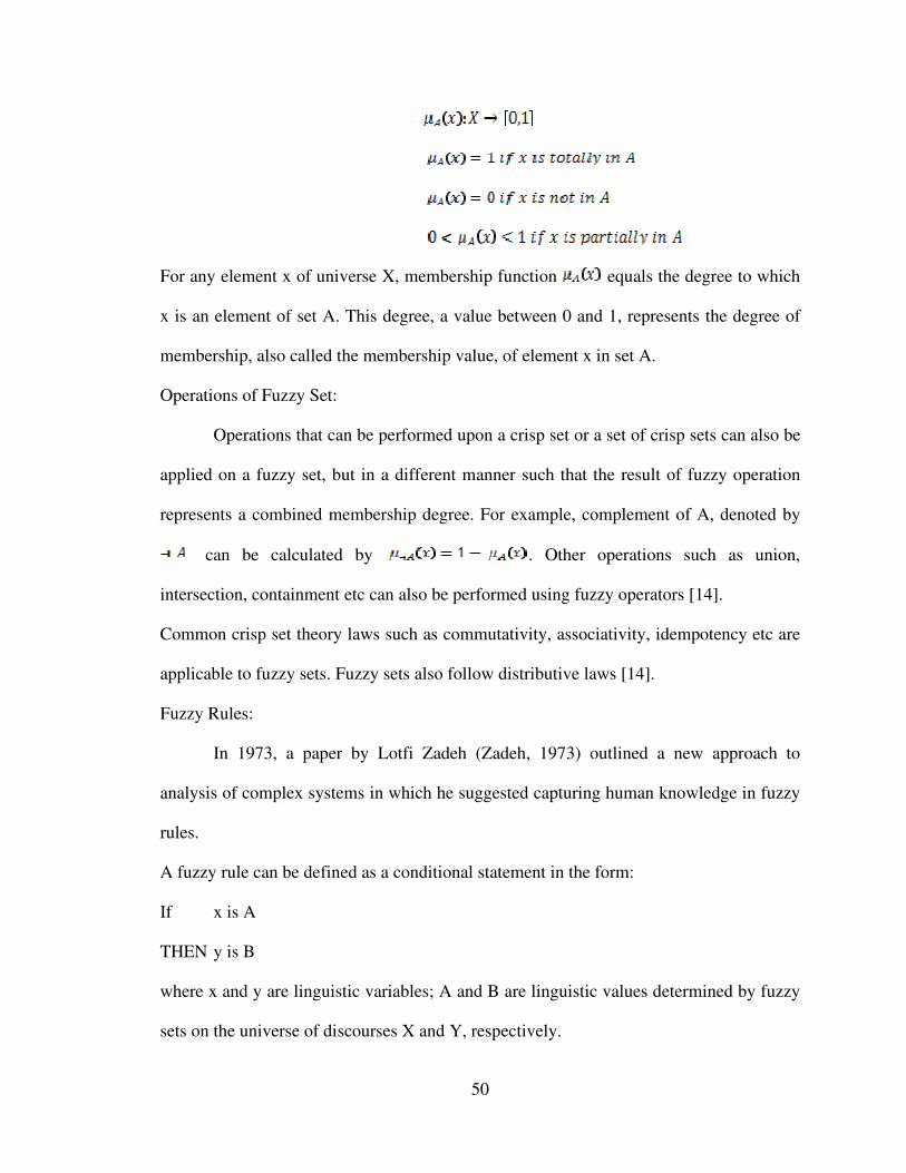
50

For any element x of universe X, membership function equals the degree to which

x is an element of set A. This degree, a value between 0 and 1, represents the degree of

membership, also called the membership value, of element x in set A.

Operations of Fuzzy Set:

Operations that can be performed upon a crisp set or a set of crisp sets can also be

applied on a fuzzy set, but in a different manner such that the result of fuzzy operation

represents a combined membership degree. For example, complement of A, denoted by

can be calculated by . Other operations such as union,

intersection, containment etc can also be performed using fuzzy operators [14].

Common crisp set theory laws such as commutativity, associativity, idempotency etc are

applicable to fuzzy sets. Fuzzy sets also follow distributive laws [14].

Fuzzy Rules:

In 1973, a paper by Lotfi Zadeh (Zadeh, 1973) outlined a new approach to

analysis of complex systems in which he suggested capturing human knowledge in fuzzy

rules.

A fuzzy rule can be defined as a conditional statement in the form:

If x is A

THEN y is B

where x and y are linguistic variables; A and B are linguistic values determined by fuzzy

sets on the universe of discourses X and Y, respectively.

51

VITA

Lakshmi Kanth Chandra Mohan

Candidate for the Degree of

Master of Science

Thesis: LAKSHMI KANTH CHANDRA MOHAN

Major Field: Computer Science

Biographical:

Personal Data:

Education:

Completed the requirements for the Master of Science in Computer Science at

Oklahoma State University, Stillwater, Oklahoma in December, 2007.

Experience:

Graduate Teaching Assistant for Computer Science Department

Student Lab Assistant for Spears School of Business

Professional Memberships:

ADVISER’S APPROVAL: Dr. Johnson Thomas

Name: Lakshmi Kanth Chandra Mohan Date of Degree: December, 2007

Institution: Oklahoma State University Location: Stillwater, Oklahoma

Title of Study: A CLUSTER BASED WIRELESS SENSOR NETWORK SECURITY

MODEL USING GAME THEORY AND RISK ASSESSMENT

Pages in Study: 51 Candidate for the Degree of Master of Science

Major Field: Computer Science

Scope and Method of Study:

The purpose of this thesis is to model an appropriate response to an attack

in a wireless sensor network by implementing game theory concepts coupled with

risk assessment. In contrast to the widely analyzed key management techniques

which involve computation and communication overhead, the security model is

designed as a non-cooperative game between the attacker and the network. By

creating and using a model that uses a risk assessment model to quantify risk and

employing a cost-payoff relation of the game theory for decision making better

resource utilization and better security can be achieved.

Findings and Conclusions:

The risk assessment model integrated with a game theoretic framework is

investigated for efficiently securing a wireless sensor network. A new

methodology to effectively estimate risk based on the threat and damage values,

using fuzzy logic has been introduced. The cost of defending a node and the

related gain in payoff with respect to the objective of the network was considered

while analyzing the game. The game model reduces the computational overhead

with nodes by moving the decision making to cluster heads. By choosing

appropriate utility parameters and payoff function the network can secure itself

efficiently.