FACTA UNIVERSITATIS (NIS)

SER.: ELEC. ENERG. vol. 22, no. 1, April 2009, 1-33

Closed-System Quantum Logic Network Implementationof the Viterbi Algorithm

Anas N. Al-Rabadi

Abstract: New convolution-based multiple-stream error-control coding and decodingschemes are introduced. The new coding method applies the reversibility propertyin the convolution-based encoder for multiple-stream error-control encoding and im-plements the reversibility property in the new reversible Viterbi decoding algorithmfor multiple-stream error-correction decoding. The complete design of quantum cir-cuits for the quantum realization of the new quantum Viterbicell in the quantum do-main is also introduced. In quantum mechanics, a closed system is an isolated systemthat can’t exchange energy or matter with its surroundings and doesn’t interact withother quantum systems. In contrast to open quantum systems,closed quantum sys-tems obey the unitary evolution and thus they are reversible. Reversibility property inerror-control coding can be important for the following main reasons: (1) reversibilityis a basic requirement for low-power circuit design in future technologies such as inquantum computing (QC), (2) reversibility leads to super-speedy encoding/decodingoperations because of the superposition and entanglement properties that emerge inthe quantum computing systems that are naturally reversible and therefore very highperformance is obtained, and (3) it is shown in this paper that the reversibility rela-tionship between multiple-streams of data can be used for further correction of errorsthat are uncorrectable using the implemented decoding algorithm such as in the caseof triple-errors that are uncorrectable using the classical irreversible Viterbi algorithm.

Keywords: Error-Correcting Codes, Error-Control Coding, Coding, Low-PowerComputing, Low-Power Circuits and Systems, Noise, QuantumCircuits, QuantumComputing, Reversible Circuits, Reversible Logic.

Manuscript received on October 12, 2008.The author is currently an Associate Professor with the Computer Engineering Department,

The University of Jordan, Jordan & is associated with the Office of Graduate Studies and Research(OGSR), Portland State University, U.S.A. (e-mail:alrabadi@yahoo.com).

1

2 A. N. Al-Rabadi:

1 Introduction

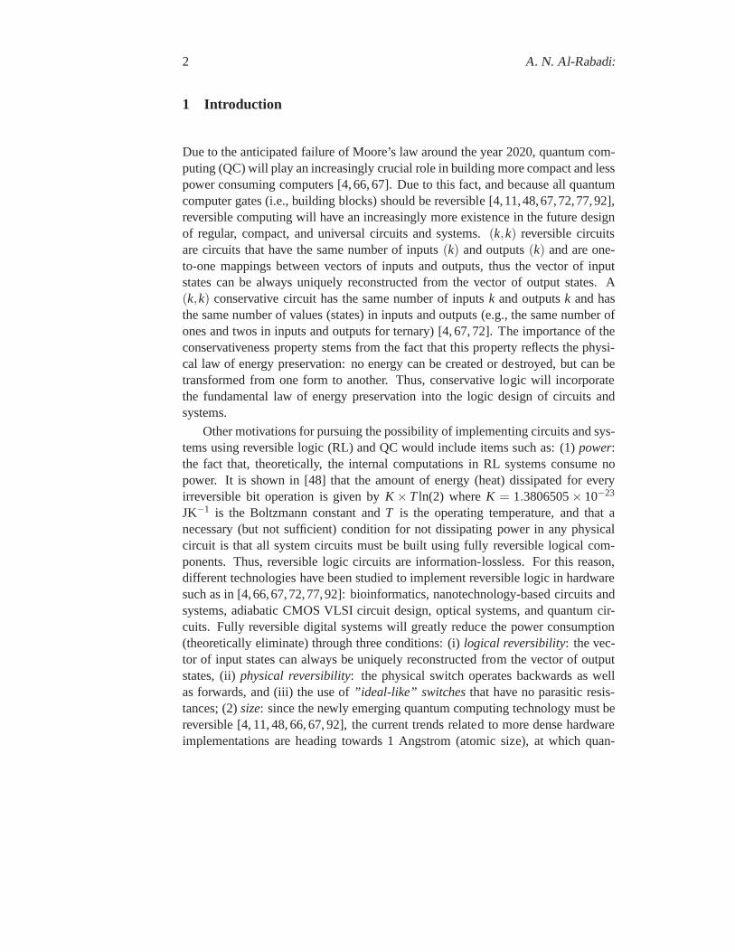
Due to the anticipated failure of Moore’s law around the year2020, quantum com-puting (QC) will play an increasingly crucial role in building more compact and lesspower consuming computers [4, 66, 67]. Due to this fact, and because all quantumcomputer gates (i.e., building blocks) should be reversible [4,11,48,67,72,77,92],reversible computing will have an increasingly more existence in the future designof regular, compact, and universal circuits and systems.(k,k) reversible circuitsare circuits that have the same number of inputs(k) and outputs(k) and are one-to-one mappings between vectors of inputs and outputs, thusthe vector of inputstates can be always uniquely reconstructed from the vectorof output states. A(k,k) conservative circuit has the same number of inputsk and outputsk and hasthe same number of values (states) in inputs and outputs (e.g., the same number ofones and twos in inputs and outputs for ternary) [4, 67, 72]. The importance of theconservativeness property stems from the fact that this property reflects the physi-cal law of energy preservation: no energy can be created or destroyed, but can betransformed from one form to another. Thus, conservative logic will incorporatethe fundamental law of energy preservation into the logic design of circuits andsystems.

Other motivations for pursuing the possibility of implementing circuits and sys-tems using reversible logic (RL) and QC would include items such as: (1)power:the fact that, theoretically, the internal computations inRL systems consume nopower. It is shown in [48] that the amount of energy (heat) dissipated for everyirreversible bit operation is given byK ×T ln(2) whereK = 1.3806505× 10−23

JK−1 is the Boltzmann constant andT is the operating temperature, and that anecessary (but not sufficient) condition for not dissipating power in any physicalcircuit is that all system circuits must be built using fullyreversible logical com-ponents. Thus, reversible logic circuits are information-lossless. For this reason,different technologies have been studied to implement reversible logic in hardwaresuch as in [4,66,67,72,77,92]: bioinformatics, nanotechnology-based circuits andsystems, adiabatic CMOS VLSI circuit design, optical systems, and quantum cir-cuits. Fully reversible digital systems will greatly reduce the power consumption(theoretically eliminate) through three conditions: (i)logical reversibility: the vec-tor of input states can always be uniquely reconstructed from the vector of outputstates, (ii)physical reversibility: the physical switch operates backwards as wellas forwards, and (iii) the use of”ideal-like” switches that have no parasitic resis-tances; (2)size: since the newly emerging quantum computing technology must bereversible [4, 11, 48, 66, 67, 92], the current trends related to more dense hardwareimplementations are heading towards 1 Angstrom (atomic size), at which quan-

Closed-System Quantum Logic Network Implementation... 3

tum mechanical effects have to be accounted for; and (3)speed (performance):if the properties of superposition and entanglement of quantum mechanics can beusefully employed in the design of circuits and systems, significant computationalspeed enhancements can be expected [4,67].

Therefore, while in the classical (irreversible) systems the frequency-to-powerratio ( f/p), or equivalently power-to-frequency ratio(p/ f ), doesn’t improve muchafter certain threshold (level) since the increase in frequency (i.e., more speed; bet-ter performance) leads to the increase in power consumption, this doesn’t exist inthe quantum domain; in the quantum system, speed of processing is very high (dueto the properties of quantum superposition and entanglement) and power consump-tion is inversely very low, i.e.,( f/p) → ∞ or equivalently(p/ f ) → 0.

In general, in data communications between two communicating systems(nodes), noise exists and corrupts the sent data messages, and thus noisy cor-rupted messages will be received. The corrupting noise is usually sourced fromthe communication channel. Therefore, error correction ofcommunicated dataand reversible error correction of communicated batch of data (i.e., parallel datastreams) are highly important tasks in situations where noise occurs. Many so-lutions have been classically implemented to solve for the classical error detec-tion and correction problems: (1) one solution to solve for error-control isparitychecking[30, 31] which is one of the most widely used methods for errordetec-tion in digital logic circuits and systems, in which re-sending data is performed incase error is detected in the transmitted data. This error isdetected by the paritychecker in the receiver side. Various parity-preserving circuits have been imple-mented in which the parity of the outputs matches that of the inputs, and suchcircuits can be fault-tolerant since a circuit output can detect a single error; (2)another solution to solve this highly important problem, that is to extract the cor-rect data message from the noisy erroneous counterpart, is by using various cod-ing schemes that work optimally for specific types of statistical distributions ofnoise [1–3,5–10,12–18,20–47,49–65,69–71,74–76,78–91,93–96,98–101].

For example, the manufacturers of integrated circuits (ICs) have recently startedto produce error-correcting circuits, and one such circuitis the TI 74LS636 [19]which is an 8-bit error detection and correction circuit that corrects any single-bitmemory read error and flags any two-bit error which is called single error correc-tion / double error detection (SECDED). This IC is currentlyfound in high-endcomputer systems because of the cost of implementing a system that uses error cor-rection, and the newest computer systems are now using DDR memory with error-correction code (ECC). When a single error is detected, the 74LS636 goes throughan error-correction cycle; the 74LS636 checks the single-error flag (SEF) to deter-mine whether an error has occurred, and if it has then a correction cycle causes the

4 A. N. Al-Rabadi:

single-error defect to be corrected, and if a double-error occurs then an interruptrequest is generated by the double-error flag (DEF) output. Since the introductionof the Intel Pentiumr microprocessor, the modern microprocessor design incorpo-rates the logic circuitry to detect/correct errors provided that the memory can storethe extra eight bits required for storing the ECC code, in which the ECC memoryis 72-bits wide using the eight additional bits to store the ECC code (i.e., memorywidth is 64 data bits + 8 bits for ECC code), and if an error occurs then the mi-croprocessor runs the correction cycle to correct the error. Recently, some memorydevices such as Samsungr memory also perform an internal error check in whichSamsungr ECC uses three bytes to check every 256 bytes of memory.

The main contributions of this paper are the introduction ofnew convolution-based multiple-stream error-control encoding and decoding schemes that apply thereversibility property in both the convolution-based encoder for multiple-streamerror-control encoding and in the new reversible Viterbi decoding algorithm formultiple-stream error-control decoding. Also, the complete design of quantum cir-cuits for the quantum implementation of the new quantum Viterbi cell (i.e., quan-tum trellis node) in the quantum domain is introduced. It is also introduced in thispaper that the reversibility relationship between multiple-streams of parallel datacan be used for further correction of errors that are uncorrectable using the imple-mented decoding algorithm such as in the case of triple-errors (or more) that areuncorrectable using the irreversible Viterbi algorithm.

Basic background in error-control coding, reversible logic and quantum com-puting is presented in Section 2. The new reversible error correction method in datacommunication is introduced in Section 3. The design of quantum circuits for thequantum implementation of the new quantum Viterbi cell is introduced in Section4. Conclusions and future work are presented in Section 5.

2 Fundamentals

This Section presents basic background in the topics of error-correction coding, re-versible logic, and quantum computing. The fundamentals presented in this sectionwill be utilized in the development of the new results introduced in Sections 3−4.

2.1 Error correction

In the data communication context, noise usually exists andis generated from thechannel in which transmitted data are communicated. Such noise corrupts sentmessages from one end and thus noisy corrupted messages are received on theother end. To solve the problem of extracting a correct message from its corrupted

Closed-System Quantum Logic Network Implementation... 5

S R

N

Stream1 Stream1'1

Stream2' Stream2

noise

C

S RN

encoder1

encoder2decoder1

decoder2

noise

Stream1 Stream1'1

Stream2Stream2'2

C

Sr

Rr

N

encoder1

encoder2decoder1

decoder2

noise

Stream1 Stream1'

Stream2Stream2'

C

Reverser Reverser

Sr

Rr

N

enc1/mod1

mod2/enc2dec1/demod1

Demod2/dec2

noise

Stream1 Stream1'

Stream2Stream2'

C

Reverser Reverser

(a) (b)

(c) (d)

Fig. 1. Modeling data communication in the existence of noise: (a) model of a noisy datacommunication where C is the channel, (b) model of the solution to the noise problem using en-coder / decoder schemes, (c) the application of reversibility using the reverser block for parallelmultiple-input multiple-output (MIMO) bijectivity (uniqueness) in the data streams, and (d) thecommunication model in which coding and modulation are combined. In this model, stream1’= stream1 + noise and stream2’ = stream2 + noise.

counterpart, noise must be modeled [22, 68, 97] and accordingly an appropriateencoding / decoding communication schemes must be implemented [1–3,5–10,12–18, 20–47, 49–65, 69–71, 74–76, 78–91, 93–96, 98–101]. Various coding schemeshave been proposed and one very important family is the convolutional codes [1–3,5,12,17,21,26,32,35,37,39,44,47,49,50,54,56,60,61,63,71,74,79,87,89,91,93,94,96,98,99]. Figure 1 illustrates the modeling of data communication in the existenceof noise, the solution to the noise problem using an encoder /decoder scheme, andthe utilization of a new block called the reverser for bijectivity (uniqueness) inmultiple-stream (i.e., parallel data) communication.

Each of the two nodes sides in the system shown in Figure 1 consists of threemajor parts: (1) encoding (e.g., generating a convolutional code using a convolu-tional encoder) to generate an encoded transmitted decision (message), (2) channelnoise, and (3) decoding (e.g., generating the correct convolution code using thecorresponding decoding algorithm (cf. Viterbi algorithm)) to generate the decodedcorrect received data message.

In general, in block coding, the encoder receives ak-bit message block and gen-erates ann-bit code word, and therefore code words are generated on a block-by-block basis, and the whole message block must be buffered before the generationof the associated code word. On the other hand, message bits are received seriallyrather than in blocks where it is undesirable to use a buffer.In such case, one usesconvloutional coding, in which a convolutional coder generates redundant bits by

6 A. N. Al-Rabadi:

using modulo-2 convolutions.

The binary convolutional encoder can be seen as a finite statemachine (FSM)consisting of anM-stage shift register with interconnections ton modulo-2 addersand a multiplexer to serialize the outputs of the adders, in which anL-bit messagesequence generates a coded output sequence of lengthn(L+M) bits [1–3,5,12,17,21,26,32,35,37,39,44,47,49,50,54,56,60,61,63,71,74,79,87,89,91,93,94,96,98,99].

Definition 1. For anL-bit message sequence,M-stage shift register,n modulo-2 adders, and a generated coded output sequence of lengthn(L+M) bits, the coderater is calculated as:

r =L

n(L+M)bits / symbol

and for the typical case ofL ≫ M, the code rate reduces tor ≈ (1/n) bits/symbol.

Definition 2. The constraint length of a convolutional code is the number ofshifts over which a single message bit can influence the encoder output. Thus,for an encoder with anM-stage shift register, the number of shifts required for amessage bit to enter the shift register and then come out of itis equal toK = M +1.Thus, the encoder constraint length is equal toK.

A binary convolutional code can be generated with code rater ≈ (k/n) by usingk shift registers,n modulo-2 adders, an input multiplexer, and an output multiplexer.An example of a convolutional encoder with constraint length = 3 and rate =1/2 isthe one shown in Figure 2.

Output

Modulo-2 adder

Path #1

Path #2

Flip-flop

Input

Modulo-2 adder

Flip-flop

Fig. 2. Convolutional encoder with constraint length = 3 andrate =1/2. The flip-flopis a unit-delay element, and the modulo-2 adder is the logic Boolean difference (XOR)operation.

The convolutional codes generated by the encoder in Figure 2are part of what isgenerally callednonsystematic codes. Each path connecting the output to the inputof a convolutional encoder can be characterized in terms of the impulse responsewhich is defined as the response of that path to “1” applied to its input, with eachflip-flop of the encoder set initially to “0”. Equivalently, we can characterize each

Closed-System Quantum Logic Network Implementation... 7

path in terms of a generator polynomial defined as the unit-delay transform of theimpulse response. More specifically, the generator polynomial is defined as:

g(D) =M

∑i=0

giDi (1)

where gi is the generator coefficients∈ {0,1}, and the generator sequence{g0,g1, . . . ,gM} composed of generator coefficients is the impulse response of thecorresponding path in the convolutional encoder, andD is the unit-delay variable.

Example 1. For the convolutional encoder in Figure 2, path #1 impulse re-sponse is (1, 1, 1), and path #2 impulse response is (1, 0, 1). Thus, according toEquation (1), the following are the corresponding generating polynomials, respec-tively, where addition is performed in modulo-2 addition arithmetic:

g1(D) = 1·D0+1·D1+1·D2

= 1+D+D2

g2(D) = 1·D0+0·D1+1·D2

= 1+D2

For a message sequence (10011), the following is theD-domain polynomial repre-sentation:

m(D) = 1·D0 +0·D1+0·D2+1·D3+1·D4

= 1+D3+D4

As convolution in time domain is transformed into multiplication in theD-domain,path #1 output polynomial and path #2 output polynomial are as follows, respec-tively:

c1(D) = g1(D)m(D) = (1+D+D2)(1+D3 +D4)

= 1+D+D2+D3+D6

c2(D) = g2(D)m(D) = (1+D2)(1+D3+D4)

= 1+D2+D3+D4+D5+D6

Therefore, the output sequences of paths #1 and #2 are as follows, respectively:

Output sequence of path #1: (1111001)Output sequence of path #2: (1011111)

The resulting encoded sequence from the convolutional encoder in Figure 2 isobtained by multiplexing the two output sequences of paths #1 and #2 as follows:

c = (11,10,11,11,01,01,11)

8 A. N. Al-Rabadi:

Example 2.For the convolutional encoder in Figure 2, the following areexam-ples of encoded data messages:

m1 = (11011) → c1 = (11010100010111)

m2 = (00011) → c2 = (00000011010111)

m3 = (01001) → c3 = (00111011111011)

In general, a data message sequence of lengthL bits results in an encoded se-quence of length equals ton(L + K − 1) bits. Usually a terminating sequence of(K −1) zeros called the tail of the message is appended to the last input bit of themessage sequence in order for the shift register to be restored to its zero initial state.

The structural properties of the convolutional encoder (cf. Figure 2) can berepresented graphically in several equivalent representations (cf. Figure 3) using:(1) code tree, (2) trellis, and (3) state diagram. The trellis contains(L + K) levelswhereL is the length of the incoming message sequence andK is the constraintlength of the code. Therefore, the trellis form is preferredover the code tree formbecause the number of nodes at any level of the trellis does not continue to growas the number of incoming message bits increases, but ratherit remains constantat 2K−1, whereK is the constraint length of the code. Figure 3 shows the variousgraphical representations for the convolutional encoder in Figure 2.

Therefore, any encoded output sequence can be generated from the correspond-ing input message sequence using the following equivalent methods: (1) circuit ofthe convolutional encoder (cf. Figure 2), (2) polynomial generator (cf. Examples 1and 2), (3) code tree (cf. Figure 3a), (4) trellis (cf. Figure3b), and (5) state diagram(cf. Figure 3c).

An important decoder that uses the trellis representation to correct receivederroneous messages is the Viterbi decoding algorithm [26, 89–91]. The Viterbi al-gorithm is a dynamic programming algorithm which is used to find the maximum-likelihood sequence of hidden states, which results in a sequence of observed eventsparticularly in the context of hidden Markov models (HMMs) [73]. The Viterbi al-gorithm forms a subset of information theory [1,22], and hasbeen extensively usedin a wide range of applications including speech recognition, keyword spotting,computational linguistics, bioinformatics, and in communications including digi-tal cellular, dial-up modems, satellite, deep-space and wireless local area network(LAN) communications.

The Viterbi algorithm is a maximum-likelihood decoder which is optimum fora noise type which is statistically characterized as an Additive White GaussianNoise (AWGN). This algorithm operates by computing a metricfor every possiblepath in the trellis representation. The metric for a specificpath is computed as theHamming distance between the coded sequence represented bythat path and the

Closed-System Quantum Logic Network Implementation... 9

0

1

00

11

00

11

10

01

00

11

10

01

11

00

01

10

00

11

10

01

11

00

01

10

00

11

10

01

11

00

01

10

00

1110

0111

0001

1000

1110

0111

0001

1000

1110

0111

0001

1000

1110

0111

0001

10

a

a

a

a

a

a

b

b

b

b

b

b

c

c

c

c

c

c

d

d

d

d

d

d

(a)

0011

01

10

00

10

01

10

10

10

01

01

00

01

01

11 11

10

11

00

11

.

.

.

00

00

11

01

01

00

1111

10

11

01

00

11

00

10

00

11

10

a

b

c

d

j = 0 j = 1 j = 2 j = 3 j = 4 j = 5 j = L-1 j = L j = L+1 j = L+2

00

11

01

.

.

.

.

.

.

00

(b)10

d

010110

b c

00

11

a

00

11

(c)

Fig. 3. Various representations for the circuit of the convolutional encoder in Figure 2: (a) code tree,(b) trellis, and (c) state diagram. Solid line is the input ofvalue “0” and the dashed line is the inputof value “1”. The binary label on each branch is the encoder’soutput as it moves from one state toanother. The state encoding of the states can be as{a = 00,b = 10,c = 01,d = 11}.

received sequence. For a pair of code vectorsc1 andc2 that have the same numberof elements, the Hamming distanced(c1,c2) between such a pair of code vectorsis defined as the number of locations in which their respective elements differ. Inthe Viterbi algorithm context, the Hamming distance is computed by counting howmany bits are different between the received channel symbolpair and the possiblechannel symbol pairs, in which the results can only be “0”, “1” or “2”. Therefore,for each node (i.e., state) in the trellis, the Viterbi algorithm compares the two pathsentering the node. The path with the lower metric is retainedand the other path isdiscarded. This computation is repeated for every levelj of the trellis in the rangeM ≤ j ≤ L, whereM = (K − 1) is the encoders memory andL is the length ofthe incoming message sequence. The paths that are retained are called survivor oractive paths. In some cases, applying the Viterbi algorithmleads to the followingdifficulty: when the paths entering a node (state) are compared and their metricsare found to be identical then a choice is made by making a guess (i.e., flippinga fair coin). The Viterbi algorithm is a maximum likelihood sequence estimator,and the following procedure and Examples 3 - 5 illustrate thedetailed steps for the

10 A. N. Al-Rabadi:

implementation of this algorithm [1, 2, 5, 12, 17, 21, 26, 39,40, 44, 54, 60, 61, 63, 71,89–91,96].

Algorithm Viterbi

1. Initialization step: Label the left-most state of the trellis (i.e., all zero state atlevel 0) as 0.

2. Computation step: Let j = 0,1,2, . . ., and assume at the previousj the fol-lowing is performed:

(a) All survivor paths are identified;(b) The survivor paths and its metric for each state of the trellis are stored.

Then, at level (clock time)( j +1) and for all the paths entering each state ofthe trellis, compute the metric by adding the metric of the incoming branchesto the metric of the connecting survivor path from levelj. Thus, for eachstate, identify the path with the lowest metric as the survivor of step( j +1),therefore updating the computation.

3. Final step: Continue the computation until the algorithm completes the for-ward search through the trellis and thus reaches the terminating node (i.e.,all zero state), at which time it makes a decision on the maximum-likelihoodpath. Then, the sequence of symbols associated with that path is released tothe destination as the decoded version of the received sequence.

Example 3. Suppose that the resulting encoded sequence from the convolu-tional encoder in Figure 2 is as follows:

c = (0000000000)

Now suppose a noise corrupts this sequence, and the noisy received sequence is asfollows:

c′ = (0100010000)

Using the Viterbi algorithm, Figure 4 shows the resulting step-by-step illustration[39] to produce the survivor path which generates the correct sent messagec =(0000000000).

Example 4. For the convolutional encoder in Figure 2, path #1 impulse re-sponse is (1, 1, 1), and path #2 impulse response is (1, 0, 1). Thus, the followingare the corresponding generating polynomials, respectively:

g1(D) = 1·D0 +1·D1+1·D2

= 1+D+D2

g2(D) = 1·D0 +0·D1+1·D2

= 1+D2

Closed-System Quantum Logic Network Implementation... 11

01

1

01Received sequence

j = 1

001 1

1

00 1

3

2

2

Received sequence

j = 2

001 1

1

00 1

3

2

2

Received sequence

j = 3

01 2

3

2

3

5

2

34

01

1

1

3

2j = 3 Survivors

2

2

2

3

001 1

1

00 1

3

2

Received sequence

j = 4

01 2

2

2

3

00 2

4

4

2

3

4

34

01

1

1

2j = 4 Survivors

2

2

2

2

2

3

3

001 1

1

00 1

2

Received sequence

j = 5

01 2

2

2

00 2

2

3

3

00 2

5

4

3

3

4

34

01

1

1

2j = 5 Survivors

2

2

2

2

2

3

2

3

3

3

Fig. 4. The illustration of the steps of the Viterbi algorithm when applied for Example 3, wherethe bold path (in levelj = 5) is the survivor path.

For a message sequence (101), the following is theD-domain polynomial represen-tation:

m(D) = 1·D0 +0·D1+1·D2

= 1+D2

12 A. N. Al-Rabadi:

As convolution in time domain is transformed into multiplication in theD-domain,the path #1 output polynomial and path #2 output polynomial are as follows, re-spectively, where addition is performed in modulo-2 arithmetic:

c1(D) = g1(D)m(D) = (1+D+D2)(1+D2)

= 1+D+D3+D4

c2(D) = g2(D)m(D) = (1+D2)(1+D2)

= 1+D4

Therefore, the output sequences of paths #1 and #2 are as follows, respectively:

Output sequence of path #1: (11011)Output sequence of path #2: (10001)

The resulting encoded sequence from the convolutional encoder in Figure 2 is ob-tained by multiplexing the two output sequences of paths #1 and #2 as follows:

c = (11,10,00,10,11)

Now suppose a noise corrupts this sequence, and the noisy received sequence is asfollows:

c′ = (01,10,10,10,11)

Using the Viterbi algorithm, the following is the resultingsurvivor path which gen-erates the correct sent messagec = (11,10,00,10,11).

j = 0

11

1

1

11

j = 4 j = 5j = 2 j = 3j = 1

1000101

2

2

2

3

2

3

2

23

3

3

3

33

4

4

4

4

Fig. 5. The resulting survivors of the Viterbi algorithm when applied forExample 4, where the bold path is the survivor path.

A difficulty with the application of the Viterbi algorithm occurs when the re-ceived sequence is very long. In this case the Viterbi algorithm is applied to atruncated path memory using a decoding window of length greater or equal five

Closed-System Quantum Logic Network Implementation... 13

times the convolutional code constraint lengthK, in which the algorithm operateson a frame-by-frame of the received sequence each of lengthl ≥ 5K. The decodingdecisions made in this way are not a truly maximum likelihood, but they can bemade almost as good provided that the decoding window is longenough. Anotherdifficulty is the number of errors; for example, in case of three errors, the Viterbi al-gorithm when applied to a convolutional code ofr = 1/2 andK = 3 cannot producea correctable decoded message from the incoming erroneous message. Exceptionsare triple-error patterns that spread over a time span> K.

Example 5. Suppose an all-zero sequencec = (0000000000) is generated bythe convolutional encoder in Figure 2. For a received sequence containing threeerrorsc′ = (1100010000), Figure 6 shows the breakdown of the Viterbi algorithmwhen implemented to the convolutional encoder in Figure 2 (K = 3 andr = 1/2)as it fails to correct for a triple-error pattern.

1

1

2

23

3

3

3

11 00 01 00Received Sequence

j = 0 j = 4j = 2 j = 3j = 1

0

Fig. 6. The illustration of the failure of the Viterbi algorithm in Example 5,where the correct path has been eliminated in levelj = 3.

2.2 Reversible logic

In quantum mechanical systems, a closed system is an isolated system that doesn’texchange energy or matter with its surroundings (i.e., doesn’t dissipate power) anddoesn’t interact with other quantum systems. Closed quantum systems obey theunitary evolution and therefore they are reversible.

In general, an(n,k) reversible circuit is a circuit that hasn number of inputsandk number of outputs and is one-to-one mapping between vectorsof inputs andoutputs, thus the vector of input states can be always uniquely reconstructed fromthe vector of output states [4,11,48,66,67,72,77,92]. Thus, a(k,k) reversible map

14 A. N. Al-Rabadi:

is a bijective function which is both (1) injective (one-to-one or (1:1)) and (2) sur-jective (onto). (Such bijective systems are also known as: equipollent, equipotent,and one-to-one correspondence.) The auxiliary outputs that are needed only forthe purpose of reversibility are called garbage outputs. These are auxiliary outputsfrom which a reversible map is constructed (cf. Example 6). Therefore, reversiblecircuits (systems) are information-lossless.

Geometrically, achieving reversibility leads to value space-partitioning thatleads to spatial partitions of unique values. Algebraically and in terms of sys-tems representation, reversibility leads to multi-input multi-output (MIMO) bijec-tive maps (i.e., bijective functions). An algorithm calledreversible Boolean func-tion (RevBF) that produces a reversible form from an irreversible Boolean functionis as follows [4].

Algorithm RevBF

1. To achieve(k,k) reversibility, add sufficient number of auxiliary outputvariables such that the number of outputs equals the number of inputs. Al-locate a new column in the mapping table for each auxiliary variable.

2. For construction of the first auxiliary output, assign a constantC1 to halfof the cells in the corresponding table column (e.g., zeros), and the secondhalf as another constantC2 (e.g., ones). For convenience, one may assignC1 to the first half of the column, andC2 to the second half of the column(cf. Table 1a, columnW1).

3. For the next auxiliary output,If non-reversibility still exists,Then assignfor identical output tuples (irreversible map entries) values which are halfzeros and half ones, and then assign a constant for the remainder that arealready reversible.

4. Do step 3 until all map entries are reversible.

Example 6. The standard two-variable Boolean equivalence (XNOR):W = c⊗ d is irreversible. The following table lists the mapping components:

c d W

0 0 10 1 01 0 01 1 1

Applying the above RevBF algorithm, the following are four possible reversibletwo-variable Boolean maps for the XNOR function:

Closed-System Quantum Logic Network Implementation... 15

Table 1. Four possible (2, 2) reversible maps for the BooleanXNOR (Boolean equivalence).

c d W W1

0 0 1 00 1 0 01 0 0 11 1 1 1

c d W W1

0 0 1 10 1 0 11 0 0 01 1 1 0

c d W W1

0 0 1 00 1 0 11 0 0 01 1 1 1

c d W W1

0 0 1 10 1 0 01 0 0 11 1 1 0

(a) (b) (c) (d)

For example, using the RevBF algorithm, the construction ofthe reversiblemap in Table 1a is obtained as follows: sinceW is irreversible, assign auxiliary(“garbage”) outputW1 and assign the first half of its values the constant “0” andthe second half another constant “1”. The new XNOR map is now reversible. Thisgate is also called the inverted Feynman gate or inverted Controlled-NOT (invertedC-NOT) gate in which:W1 = c andW = c⊗ d = (c⊕ d)′ (cf. Feynman gate inFigure 11a.)

2.3 Quantum computing

Quantum computing (QC) is a method of computation that uses aclosed-systemdynamic process governed (for a single particle) by the Schroinger Equation (SE)[4, 67]. The single-particle one-dimensional time-dependent SE (TDSE) takes thefollowing general form:

−(h/2π)2

2m∂ 2|ψ〉∂x2 +V|ψ〉 = i

h2π

∂ |ψ〉∂ t

(2)

or

H|ψ〉= i~∂ |ψ〉

∂ t(3)

where h is Planck constant (6.626×10−34 Js), ~ = h/(2π) is the reducedPlanck constant,V(x, t) is the potential,m is particle mass,i is the imaginarynumber, |ψ(x, t)〉 is the quantum state,H is the Hamiltonian operator (H =−[(h/2π)2/2m]∇2 + V), and ∇2 is the Laplacian operator. While the aboveholds for all physical systems, in the quantum computing (QC) context, the time-independent SE (TISE) is normally used [4,67]:

∇2|ψ〉 =2m~2 (V −E)|ψ〉 (4)

where the solution|ψ〉 is an expansion over orthogonal basis states|φi〉 defined inHilbert spaceH as follows:

|ψ〉 = ∑i

ci |φi〉 (5)

16 A. N. Al-Rabadi:

where the coefficientsci are called probability amplitudes, and|ci |2 is the probabil-ity that the quantum state|ψ〉 will collapse into the (eigen) state|φi〉. The proba-bility is equal to the inner product|〈φi |ψ〉|2, with the unitary condition∑ |ci |2 = 1.

In QC, a linear and unitary operatorT is used to transform an input vector ofquantum bits(qubits) into an output vector of qubits [4, 67]. In two-valued QC, aqubit is a vector of bits defined as follows:

qubit0 ≡ |0〉 =

[

10

]

, qubit1 ≡ |1〉 =

[

01

]

(6)

A two-valued quantum state|ψ〉 is a superposition of quantum basis states|φ1〉such as those defined in Equation (6). Thus, for the orthonormal computationalbasis states{|0〉, |1〉}, one has the following quantum state:

|ψ〉 = α |0〉+ β |1〉 (7)

whereαα∗ = |α |2 = p0 ≡ the probability of having state|ψ〉 in state|0〉, ββ ∗ =|β |2 = p1 ≡ the probability of having stateψ〉 in state|1〉, and|α |2+ |β |2 = 1. Thecalculation in QC for multiple systems (e.g., the equivalent of a register) follow thetensor product (⊗) [4]. For example, given two states|ψ1〉 and |ψ2〉 one has thefollowing QC:

|ψ12〉 = |ψ1ψ2〉 = |ψ1〉⊗ |ψ2〉= (α1|0〉+ β1|1〉)⊗ (α2|0〉+ β2|1〉)= α1α2|00〉+ α1β2|01〉+ β1α2|10〉+ β1β2|11〉

(8)

A physical system, describable by the following equation [4,67]:

|ψ〉 = c1|Spinup〉+c2|Spindown〉 (9)

(e.g., the hydrogen atom), can be used to physically implement a two-valued QC.Another common alternative form of Equation (9) is:

|ψ〉 = c1

∣

∣

∣+

12

⟩

+c2

∣

∣

∣− 1

2

⟩

(10)

Many-valued QC (MVQC) can also be accomplished [4, 67]. For the three-valued QC, thequbit becomes a 3-dimensional vectorqudit (quantum discretedigit), and in general, for MVQC the qudit is of dimension many. Forexample,one has for 3-state QC (in Hilbert spaceH) the following qudits:

qudit0 ≡ |0〉 =

100

, qudit1 ≡ |1〉 =

010

, qudit2 ≡ |2〉 =

001

(11)

Closed-System Quantum Logic Network Implementation... 17

A three-valued quantum state is a superposition of three quantum orthonor-mal basis states (vectors). Thus, for the orthonormal computational basis states{|0〉, |1〉, |2〉}, one has the following quantum state:

|ψ〉 = α |0〉+ β |1〉+ γ |2〉 (12)

whereαα∗ = |α |2 = p0 ≡the probability of having state|ψ〉 in state|0〉, ββ ∗ =|β |2 = p1 ≡the probability of having state|ψ〉 in state|1〉, γγ∗ = |γ |2 = p2 ≡theprobability of having state|ψ〉 in state|2〉, and|α |2 + |β |2 + |γ |2 = 1.

In general, for ann-valued logic, a quantum state is a superposition ofn quan-tum orthonormal basis states (vectors). Thus, for the orthonormal computationalbasis states{|0〉, |1〉, . . . , |n−1〉}, one has the following quantum state:

|ψ〉 =n−1

∑k=0

ck|q〉k (13)

where:∑n−1k=0 ckc∗k = ∑n−1

k=0 |ck|2 = 1.

The calculation in QC for many-valued multiple systems follow the tensorproduct in a manner similar to the one demonstrated for two-valued QC in Equation(8).

As stated previously, while an open quantum system does interact with its en-vironment (i.e., its surroundings or bath) and thus dissipate power resulting in anon-unitary evolution, a closed quantum system is an isolated system that doesn’texchange energy or matter with its surroundings and therefore doesn’t dissipatepower resulting in a unitary evolution (i.e., unitary transformation or unitary ma-trix) and hence they are reversible. A physical system comprising trapped ionsunder multiple laser excitations can be used to reliably implement MVQC [66]. Aphysical system in which an atom (particle) is exposed to a specific potential field(function)V(x) can also be used to implement MVQC (two-valued being a specialcase) [4, 67]. In such an implementation, the (resulting)distinct energy statesareused as the orthonormal basis states. The latter is illustrated in Example 7 belowwhich is an example of implementing MVQC by exposing a particle to a potentialfieldV where the distinct energy states are used as theorthonormal basis states.

Example 7. We assume the following constraints: (1) spring potentialV(x) =(1/2)kx2, wherem is a particle,k = mω2 is spring constant, andω is the angularfrequency (ω = 2π· frequency), and (2) boundary conditions. Also, assuming thesolution of the TISE in Equation (4) for these constraints isof the following form(i.e., the Gaussian function):

ψ(x) = Ce−α x22

18 A. N. Al-Rabadi:

whereα = mω/~. The general solution for the wave function|ψ〉, (for a springpotential) is:

C =[α

π

]14 1√

2nn!Hn(

√αx)

whereHn(x) are the Hermite polynomials. This solution leads to the sequence ofevenly spaced energy levels (eigenvalues)En characterized by a quantum numbern as follows:

En = (n+12)~ω

The distribution of the energy states (eigenvalues) and their associated proba-bilities are shown in Figure 7.

Fig. 7. Harmonic oscillator (HO) potential and wavefunctions: (a) wavefunctions for variousenergy levels (subscripts), (b) spring potentialV(x) and the associated energy levelsEn, and (c)probabilities for measuring particlem in each energy state (En).

A closed-system quantum circuit is a composition of quantumgates with thefollowing properties [4, 67]: (1) must be reversible, (2) must have an equal num-ber of inputsk and outputsk, (3) doesn’t allow fan-out, (4) is constrained to beacyclic (i.e., feedback (loop) is not allowed), and (5) the transformation performedis unitary (i.e., a unitary matrix). The quantum Viterbi circuit design in the quan-tum domain using the corresponding basic quantum primitives will be completelyshown in Section 4.

Closed-System Quantum Logic Network Implementation... 19

3 Reversible Error Correction via Reversible Viterbi Algor ithm

While in subsection 2.1 the error correction of communicated data was done forthe case of single-input single-output (SISO) systems, this section introduces re-versible error correction of communicated batch (parallel) of data in multiple-inputmultiple-output (MIMO) systems. Reversibility in parallel-based data communica-tion is directly observed since:

~O1 = ~I2 (14)

where~O1 is theuniqueoutput (transmitted) data from node #1 and~I2 is theuniqueinput (received) data to node #2.

In MIMO systems, the existence of noise will cause an error that may lead toirreversibility in data communication (i.e., irreversibility in data mapping) since~O1 6= ~I2. As will be introduced in this and the following sections respectively,the implementation of reversible error correction can be performed (1) in softwareusing the new reversible error-correction algorithm and (2) in hardware using quan-tum error correction hardware. The following algorithm, called Reversible Viterbi(RV) Algorithm, introduces the implementation of reversible error correction in theparallel data communication.

Algorithm RV

1. Use the RevBF Algorithm to reversibly encode the communicated batch ofdata.

2. Given a specific convolutional encoder circuit, determine the generatorpolynomials for all paths.

3. For each communicated message within the batch, determine the encodedmessage sequence.

4. For each received message, use the Viterbi Algorithm to decode the re-ceived erroneous message.

5. Generate the total maximum-likelihood trellis resulting from the iterativeapplication of the Viterbi decoding algorithm.

6. Generate the corrected communicated batch of data messages.7. End

The convolutional encoding for the RV algorithm can be performedserially us-ing a single convolutional encoder from Figure 2, or inparallel using the generalparallel convolutional encoder circuit shown in Figure 8 inwhich severals con-volutional encoders operate in parallel for encodings number of simultaneously

20 A. N. Al-Rabadi:

.

.

.

.

.

.

.

.

.

.

.

.

.

.

Fig. 8. General MIMO encoder circuit for the parallel generation of convolutional codes whereeach box represents a single SISO convolutional encoder such as the one shown in Figure 2.

submitted messages (i.e., data message set of cardinality (size) equal tos) gener-ated fromsnodes.

Example 8. The reversibility implementation (e.g., RevBF Algorithm)uponthe following input bit stream{m1 = 1,m2 = 1,m3 = 1} produces the followingreversible set of message sequences:

m1 = (101)

m2 = (001)

m3 = (011)

For the convolutional encoder in Figure 8, the following is theD-domain polyno-mial representations, respectively:

m1(D) = 1·D0 +0·D1+1·D2 = 1+D2

m2(D) = 0·D0 +0·D1+1·D2 = D2

m3(D) = 0·D0 +1·D1+1·D2 = D+D2

The resulting encoded sequences are generated in parallel as follows, respectively:

c1 = (1110001011)

c2 = (0000111011)

c3 = (0011010111)

Now suppose noise sources corrupt these sequences, and the noisy received se-quences are as follows:

c′1 = (1111001001)

c′2 = (0100101011)

c′3 = (0010011111)

Using the RV algorithm, Figure 9 shows the resulting survivor paths which gen-erate the correct sent messages:{c1 = (1110001011), c2 = (0000111011), c3 =(0011010111)}.

Closed-System Quantum Logic Network Implementation... 21

1110

0010

11

00 00

11

10

11

00

11

0101

11

(a) (b) (c)

11 11

j = 4 j = 5j = 2 j = 3j = 0 j = 1

100010

11

00 00

11

10

00

11

0101

11

(d)

Fig. 9. The resulting survivor paths of the RV algorithm whenapplied to Example 8.

As in the irreversible Viterbi Algorithm, in some cases, applying the reversibleViterbi (RV) algorithm leads to the following difficulties:(1) when the paths enter-ing a node (state) are compared and their metrics are found tobe identical then achoice is made by making a guess (i.e., flipping a fair coin); (2) when the receivedsequence is very long and in this case the reversible Viterbialgorithm is applied toa truncated path memory using a decoding window of length greater or equal fivetimes the convolutional code constraint lengthK, in which the algorithm operateson a frame-by-frame of the received sequence each of lengthl ≥ 5K, and the de-coding decisions made in this way are not a truly maximum likelihood, but theycan be made almost as good provided that the decoding window is long enough;(3) the number of errors: for example, in case of three errors, the Viterbi algorithmwhen applied to a convolutional code ofr = 1/2 andK = 3 cannot produce a cor-rectable decoded message from the incoming erroneous noisy(corrupted) message.(Exceptions are triple-error patterns that spread over a time span> K.)

Yet, parallelism in multi-stream data submission (transmission) allows for thepossible existence of extra relationship(s) between the submitted data-streams thatcan be used for (1) detection of error existence and (2) further correction afterRV algorithm in case the RV algorithm fails to correct for theoccurring errors.Examples of such inter-stream relationships are: (1) parity (even and odd) rela-tionship between the corresponding bits within the inter-stream submitted data, (2)reversibility relationship between the parallel submitted data streams and this re-

22 A. N. Al-Rabadi:

lationship exists from applying a known reversible mappingsuch as the RevBFalgorithm, or (3) combination of parity and reversibility properties. The reversibil-ity property in the RV algorithm produces a reversibility relationship between thesent parallel streams of data, and this known reversibilitymapping can be used tocorrect the uncorrectable errors (e.g., triple errors) which the RV algorithm fails tocorrect.

Example 9. The following is a version of the RevBF algorithm that producesreversibility as follows:

Algorithm RevBF (Version 1)

1. To achieve(k,k) reversibility, add sufficient number of auxiliary outputvariables (starting from right to left) such that the numberof outputs equalsthe number of inputs. Allocate a new column in the mappings table foreach auxiliary variable.

2. For construction of the first auxiliary output, assign a constantC1 = “0” tohalf of the cells in the corresponding table column, and the second half asanother constantC2= “1”. AssignC1 to the first half of the column, andC2

to the second half of the column.3. For the next auxiliary output,If non-reversibility still exists,Then assign

for identical output tuples (irreversible map entries) values which are halfones and half zeros, and then assign a constant for the remainder that arealready reversible which is the ones complement (NOT; inversion) of thepreviously assigned constant to that remainder.

4. Do step 3 until all map entries are reversible.

For the parallel sent bit stream{1,1,1} in Example 8 in which the reversibilityimplementation (using Version 1 of the RevBF Algorithm) produces the follow-ing reversible sent set of data sequences:{m1 = (101),m2 = (001),m3 = (011)}.Suppose thatm1 and m2 are decoded correctly andm3 is still erroneous due tosubmission. Figure 10 shows possible tables in which erroneousm3 exist:

m1 1 0 1m2 0 0 1m3 0 1 1

m1 1 0 1m2 0 0 1m3 0 0 1

m1 1 0 1m2 0 0 1m3 1 1 1

m1 1 0 1m2 0 0 1m3 1 0 1

(a) (b) (c) (d)

m1 1 0 1m2 0 0 1m3 0 1 0

m1 1 0 1m2 0 0 1m3 1 0 0

m1 1 0 1m2 0 0 1m3 1 1 0

m1 1 0 1m2 0 0 1m3 0 0 0

(e) (f) (g) (h)

Fig. 10. Tables for possible errors in data streamm3 that is generated by the RevBF Algorithm V1:(a) original sent correct (uncorrupted)m3 that resulted from the application of the RevBF AlgorithmV1, and (b)–(h) possibilities of the erroneous receivedm3.

Closed-System Quantum Logic Network Implementation... 23

Note that the erroneousm3 is Figures 10b-10e and 10g-10h are correctableusing the RV algorithm since less than triple-errors exits,but the triple error as inFigure 10f is (usually) uncorrectable using the RV algorithm. Yet, the existenceof the reversibility property using the RevBF algorithm adds information that canbe used to correctm3 as follows: By applying the RevBF Algorithm (Version 1)from right-to-left in Figure 10f one notes that in the secondcolumn (from right)two “0” cells are added in the top in the correctly receivedm1 andm2 messages,which means that in the most right column the last cell must be“1” since otherwisethe top two cells in the correctly receivedm1 andm2 messages should have been“0” and “1” respectively to achieve value space-partitioning. Now, since the 3rdcell of the most right column must be “1” then the last cell of the 2nd columnfrom the right must be “1” also because of the uniqueness requirement accordingto the RevBF algorithm (Version 1) for value space-partitioning between the firsttwo messages{m1,m2} and the 3rd messagem3. Then, and according to the RevBFalgorithm (Version 1) the 3rd cell of the last column from right must have the value“0” which is the ones complement (NOT) of the previously assigned constant “1”to the 3rd cell of the 2nd column from the right. Consequently, the correct messagem3 = (011) is obtained.

4 Quantum Circuit Design of the New RV Algorithm

The reversible hardware implementation for each trellis node in the (reversible)Viterbi algorithm requires the following reversible components: reversible modulo-2 adder, reversible arithmetic adder, reversible subtractor (RS) and reversible se-lector (i.e., reversible multiplexer) to be both used in onepossible design of thecorresponding reversible comparator (RC). Table 2 shows the truth tables of an ir-reversible half-adder (HA), irreversible subtractor, andirreversible full-adder (FA).

Table 2. Truth tables: (a) irreversible half-adder (HA) andirreversible subtractor, and(b) irreversible full-adder (FA).

Inputs Half-Adder SubtractorOutputs Outputs

a b a+b Carry a−b Borrow

0 0 0 0 0 00 1 1 0 1 11 0 1 0 1 01 1 0 1 0 0

Inputs Outputsa b ci s c0

0 0 0 0 00 0 1 1 00 1 0 1 00 1 1 0 11 0 0 1 01 0 1 0 11 1 0 0 11 1 1 1 1

(a) (b)

24 A. N. Al-Rabadi:

While each quantum circuit is reversible, not each reversible circuit is quan-tum [4, 67]. Figure 11 shows the various quantum circuits forthe quantum re-alization of each quantum trellis node in the corresponding(reversible) Viterbialgorithm. Figures 11a-11c present fundamental quantum gates [4, 67]. Figures

c C = c

a A = c' a c b

b B = c' b c a

c C = c

a A = c' a c b

b B = c' b c a

Quant. XOR

Quant. XOR

QCM

QFA

QHA

a A = a

b B = a b

a A = a

b B = a b

c = 0 C = c (a b)

b B = b

c C = b c

a A = a (b c) c

a A = a

b B = b

c C = ab c

a A = a

b B = a b

c C = a b c

d = 0 D = ab bc ac

A0

A1

B0

B1

0 Q

(a) (b) (c)

(d) (e) (f)

(g) (h)

Fig. 11. Quantum reversible circuits for the quantum realization of each trellis node in the corre-sponding (reversible) Viterbi algorithm: (a) quantum XOR gate (Feynman gate; Controlled-NOT(C-NOT) gate), (b) quantum Toffoli gate (Controlled-Controlled-NOT (C2-NOT) gate), (c) quantummultiplexer (Fredkin gate; Controlled-Swap (C-Swap) gate), (d) quantum subtractor, (e) quantumhalf-adder (QHA), (f) quantum full-adder (QFA), (g) quantum equality-based comparator that com-pares two 2-bit numbers where an isolated XOR symbol means a quantum NOT gate, and (h) basicquantum reversible Viterbi (QV) cell (i.e., quantum reversible trellis node) which is made of twoFeynman gates, one QHA, one QFA and one quantum comparator with multiplexing (QCM). Thequantum comparator can be synthesized using a quantum subtractor (QS) and a Fredkin gate. Thesymbol⊕ is logic XOR (exclusive OR; modulo-2 addition),∧ is logic AND,∨ is logic OR, and′ islogic NOT.

11d-11g show basic quantum arithmetic circuits of: quantumsubtractor (Figure11d), quantum half-adder (Figure 11e), quantum full-adder(Figure 11f), and thequantum equality-based comparator (Figure 11g) [4,67]. Figure 11h introduces the

Closed-System Quantum Logic Network Implementation... 25

basic quantum Viterbi cell (i.e., quantum trellis node) which is made of two Feyn-man gates, one QHA, one QFA and one quantum comparator with multiplexing(QCM).

Figure 12 shows the logic circuit design of an iterative network to comparetwo 3-digit binary numbers:X = x1x2 x3 andY = y1 y2 y3, and Figure 13 presentsthe detailed synthesis of a comparator circuit which is madeof a comparator cell(Figure 13a) and a comparator output circuit (Figure 13b). The extension of thecircuit in Figure 12 to compare twon-digit binary numbers is straightforward byutilizing n-cells and the same output circuit.

Cell1 Cell2 Cell3Output

Circuit

x1 y1 x2 y2 x3 y3

a1 = 0

b1 = 0

a2

b2

a3

b3

a4

b4

O1 (x < y)

O2 (x = y)

O3 (x > y)

Fig. 12. An iterative network to compare two 3-digit binary numbers: X = x1x2x3 andY =y1y2y3.

ai

bi

a

(a) (b)

i+1

bi+1

yi xi

celli

an+1

bn+1

O1 (x < y)

O2 (x = y)

O3 (x > y)

Fig. 13. Designing a comparator circuit: (a) comparator cell and (b) comparator output circuit.

Figure 14 illustrates the quantum circuit synthesis for thecomparator cell andthe output circuit (which were shown in Figure 13), and Figure 15 shows the designof a quantum comparator with multiplexing (QCM) where Figure 15a shows aniterative quantum network to compare two 3-digit binary numbers and Figure 15cshows the complete design of the QCM. The extension of the quantum circuit inFigure 15a to compare twon-digit binary numbers is straightforward by utilizingn quantum cells (from Figure 14a) and the same output quantum circuit (in Figure14b).

26 A. N. Al-Rabadi:

xi

yi

0

ai

bi

0

0

0

0

0

ai+1

bi+1

an+1

bn+1

0

O1

O2

O3

(a) (b)

Fig. 14. Quantum circuit synthesis for the comparator cell and output circuit in Figure 13: (a)quantum comparator cell and (b) quantum comparator output circuit.

O1

O2

O3

x y

Quantum

Comparator

3 3

00

0

0

O1

O2

O3

0 x 0 y

Quantum

Comparator

3

3 3

3

3

3

(3)

(3) (3)

3

3 3

(a)

(b) (c)

Fig. 15. Designing a quantum comparator with multiplexing (QCM): (a) an iterative quantumnetwork to compare two 3-digit binary numbers, (b) symbol ofthe quantum comparator circuitin (a), and (c) complete design of QCM where the number 3 on lines indicates triple linesand (3) beside sub-circuits indicates triple circuits (i.e., three copies of each sub-circuit for theprocessing of the triple-input triple-output lines.)

Closed-System Quantum Logic Network Implementation... 27

Figure 16 shows the complete design of a quantum trellis node(i.e., quantumViterbi cell) in the irreversible and reversible Viterbi algorithms that was shownin Figure 11h. The design of the quantum trellis node shown inFigure 16f pro-

QHAQFA

s1s1*

s3s4

c1c1*

c

c*

A1

B1

A2

B2

0

s1

c1

A1*

B1*

A2*

B2*

0

s2

c2

s1

s1*

0c1

c1*

s4

c*

0

s3

s2

s2*

0c2

c2*

s4*

c**

0

s3*

0

0

O1

O2

O3

{s3,s4,c*} {s3

*,s4*,c**}

0 0

Quantum

Comparator

3

3 3

3

3

3

(3)

(3) (3)

3

3 3

(d) (e) (f)

(a) (b) (c)

Fig. 16. The complete design of a quantum trellis node in the irreversible and reversible Viterbialgorithms that was shown in Figure 11h: (a) quantum circuitthat is made of two Feynman gates(i.e., two quantum XORs) to produce the difference between incoming received bits (A1A2) andtrellis bits (B1B2) followed by quantum half-adder (QHA) to produce the corresponding sum(s1c1) which is the Hamming distance for the first line entering thetrellis node, (b) quantumcircuit that is made of two Feynman gates (i.e., two quantum XORs) to produce the differencebetween incoming received bits (A∗

1A∗2) and trellis bits (B∗

1B∗2) followed by quantum half-adder

(QHA) to produce the corresponding sum (s2c2) which is the Hamming distance for the secondline entering the trellis node, (c) logic circuit composed of QHA and quantum full-adder (QFA)that adds the current Hamming distance to the previous Hamming distance, (d) quantum circuitin the first line entering the trellis node for the logic circuit in (c) that is made of a QHA followedby a QFA, (e) quantum circuit in the second line entering the trellis node for the logic circuit in(c) that is made of a QHA followed by a QFA, and (f) quantum comparator with multiplexing(QCM) in the trellis node that compares the two entering metric numbers: X = s3s4c∗ andY = s∗3s∗4c∗∗ and selects using control lineO1 the path that produces the minimum enteringmetric (i.e.,X < Y).

ceeds as follows: (1) two quantum circuits for the first and second lines enteringthe trellis node each is made of two Feynman gates (i.e., two quantum XORs) toproduce the difference between incoming received bits and trellis bits followed byquantum half-adder (QHA) to produce the corresponding sum (which is the Ham-ming distance) are shown in Figures 16a and 16b, (2) logic circuit composed of aQHA and a quantum full-adder (QFA) that adds the current Hamming distance to

28 A. N. Al-Rabadi:

the previous Hamming distance is shown in Figure 16c, (3) twoquantum circuitsfor the first and second lines entering the trellis node each is synthesized accordingto the logic circuit in Figure 16c (which is made of a QHA followed by a QFA) areshown in Figures 16d and 16e, (4) quantum comparator with multiplexing (QCM)in the trellis node that compares the two entering metric numbers (i.e., two enteringHamming distances) and selects using the control lineO1 the path that producesthe minimum entering metric (i.e., minimum entering Hamming distance) is shownin Figure 16f.

In Figures 16c-16e, the current Hamming metric{s1, c1} for the first enteringpath of the trellis node and the current Hamming metric{s2, c2} for the secondentering path of the trellis node is always made of two bits (00, 01, or 10). Ifmore than two digits (two bits) is needed to represent the previous Hamming met-ric for the first or second entering paths of the trellis node (e.g.,(5)10 = (101)2),then extra QFAs are added in the logic circuit in Figure 16c and consequently inthe quantum circuits shown in Figures 16d-16e. Also, in the case that when thepaths entering a quantum trellis node (state) are compared and their metrics arefound to be identical then a choice is made by making a guess tochoose any ofthe two entering paths, and this is automatically performedin the quantum circuitin Figure 16f since if ({s3, s4,c∗} < {s∗3, s∗4,c

∗∗}) thenO1 =“1” and thus choosesX = {s3, s4, c∗}, elseO1 =“0” and then it choosesY = {s∗3, s∗4, c∗∗} in both casesof ({s3, s4, c∗} > {s∗3, s∗4, c∗∗}) or ({s3, s4, c∗} = {s∗3, s∗4, c∗∗}).

5 Conclusions and Future Work

This paper introduces new convolution-based multiple-stream error-correction en-coding and decoding methods that implement the reversibility property in theconvolution-based encoder for multiple-stream error-control encoding and in thenew reversible Viterbi (RV) decoding algorithm for multiple-stream error-controldecoding. This paper also introduces the complete synthesis of quantum circuitsin the quantum domain for the quantum implementation of the new quantum trellisnode (i.e., quantum Viterbi cell). It is also shown in this paper that the relationshipof reversibility in multiple-streams of communicated parallel data can be used forfurther correction of errors that are uncorrectable using the implemented decodingalgorithm such as in the cases of the failure of the RV algorithm in correcting formore than two errors.

While an open quantum system interacts with its environment(i.e., its sur-roundings or bath) and thus dissipates power which result ina non-unitary evo-lution, a closed quantum system doesn’t exchange energy or matter with its sur-roundings and therefore doesn’t dissipate power which results in a unitary evolution

Closed-System Quantum Logic Network Implementation... 29

(i.e., unitary matrix) and hence it is reversible. Since power reduction has becomethe current main concern for digital logic designers after performance (speed), re-versibility property in error-control coding is highly important because reversibilityis a main requirement for low-power circuit synthesis of future technologies suchas in quantum computing, and reversibility property results in super-speedy encod-ing/decoding operations because of the superposition and entanglement propertiesthat emerge in the closed quantum computing systems that areinherently reversible.

Future work will include items such as the investigation of using the introducedreversibility property in more advanced multi-error coding schemes to correct thecorresponding corrupted multi-stream communicated data,and also the investiga-tion of the corresponding optimal quantum circuit design ofsuch new reversiblesystems.

References

[1] N. Abramson,Information theory and coding, McGraw-Hill, New York, 1963.[2] J. J. Adamk,Foundations of coding, Wiley, New York, 1991.[3] Y. Akaiwa, Introduction to digital mobile communication, Wiley, New York, 1997.[4] A. N. Al-Rabadi,Reversible logic synthesis: From fundamentals to quantum com-

puting, Springer-Verlag, New York, 2004.[5] J. B. Anderson and S. Mohan,Source and channel coding: An algorithmic ap-

proach, Kluwer Academic, Boston, Mass., 1991.[6] J. B. Anderson and D. P. Taylor,A bandwidth-efficient class of signal space codes,

IEEE Transactions on Information TheoryIT-24 (1978), 703–712.[7] B. S. Atal and M. R. Schroeder,Stochastic coding of speech signals at very low bit

rates, IEEE International Conference on Communications, May 1984.[8] L. R. Bahi, J. Cocke, F. Jelinek, and J. Raviv,Optimal decoding of linear codes

for minimizing symbol error rate, IEEE Transactions on Information TheoryIT-20(1974), 284–287.

[9] G. Battail, Coding for the Gaussian channel: the promise of weighted output de-coding, International J. Satellite Communications7 (1989), 183–192.

[10] S. Benedetto and G. Montorsi,Unveiling turbo codes: Some results on parallelconcatenated coding schemes, IEEE Transactions on Information Theory42(1996),409–428.

[11] C. Bennett,Logical reversibility of computation, IBM Journal of Research and De-velopment17 (1973), 525 – 532.

[12] E. R. Berlekamp,Algebraic coding theory, McGraw-Hill, New York, 1968.[13] C. Berrou and A. Glavieux,Near optimum error correcting coding and decoding:

Turbo codes, IEEE Transactions on Communications44 (1996), 1261–1271.[14] , Reflections on the prize paper: Near optimum error-correcting coding

and decoding turbo codes, IEEE Information Theory Society Newsletter48 (1998),no. 2, 24 – 31.

[15] C. Berrou, A. Glavieux, and P. Thitmajshima,Near Shannon limit error-correctioncoding and decoding: Turbo codes, International Conference on Communications(Geneva, Switzerland), May 1993, pp. 1064–1090.

30 A. N. Al-Rabadi:

[16] V. K. Bhargava,Forward error correction schemes for digital communications,IEEE Communications Magazine21 (1983), no. 1, 11–19.

[17] V. K. Bhargava, D. Haccoun, R. Matyas, and P. Nuspl,Digital communications bysatellite: Modulation, multiple access, and coding, Wiley, New York, 1981.

[18] R. C. Bose and D. K. Ray-Chaudhuri,On a class of error correcting binary groupcodes, Information and Control3 (1960), 68–79.

[19] Barry B. Brey,The intel microprocessors: Architecture, programming, and inter-facing, 7th ed., Pearson Education Inc., 2006.

[20] A. Buzo, A. H. Gray, Jr., R. M. Gray, and J. D. Markel,Speech coding based uponvector quantization, IEEE Transactions on Acoustics, Speech, and Signal Process-ing ASSP-28(1980), 562–574.

[21] G. C. Clark, Jr. and J. B. Cain,Error-correction coding for digital communications,Plenum Publishers, New York, 1981.

[22] T. M. Cover and J. A. Thomas,Elements of information theory, Wiley, New York,1991.

[23] F. Daneshgaran and M. Mondin,Design of interleavers for turbo codes: Iterativeinterleaver growth algorithms of polynomial complexity, IEEE Transactions on In-formation Theory45 (1999), 1845–1859.

[24] D. Divsalar,Turbo codes, MILCOM tutorial (San Diego), November 1996.[25] P. Elias,Coding for noisy channels, IRE Convention Record, Part 4 (1955), 37–46.[26] G. D. Forney, Jr.,The Viterbi algorithm, Proceedings of the IEEE61 (1973), no. 3,

268–278.[27] G. D. Forney, Jr. and M. V. Eyuboglu,Combined equalization and coding using

precoding, IEEE Communications Magazine29 (1991), no. 12, 25–34.[28] B. J. Frey and D. J. C. MacKay,Irregular turbocodes, Proceedings of the 37th

Annual Allerton Conference on Communication, Control, andComputing (AllertonHouse, Illinois), September 1999.

[29] D. Gabor,Theory of communication, Journal of IEE93 (1946), 429–457, Part III.[30] R. G. Gallager,Low-density parity-check codes, IRE Transactions on Information

Theory8 (1962), 21–28.[31] , Low-density parity-check codes, M.I.T. Press, Cambridge, Mass., 1963.[32] R. D. Gitlin, J. F. Hayes, and S. B. Weinstein,Data communications principles,

Plenum, New York, 1992.[33] M. J. E. Golay,Note on digital coding, Proceedings of the IRE37 (1949), 657.[34] , Binary coding, IRE Transactions on Information TheoryPGIT-4 (1954),

23 – 28.[35] S. W. Golomb,Shift register sequences, Holden-Day, San Francisco, 1967.[36] D. W. Hagelbarger,Recurrent codes: Easily mechanized burst-correcting binary

codes, Bell System Tech. J.38 (1959), 969 – 984.[37] J. Hagenauer, E. Offer, and L. Papke,Iterative decoding of binary block and convo-

lutional codes, IEEE Transactions on Information Theory42 (1996), 429 – 445.[38] R. W. Hamming,Error detecting and error correcting codes, Bell System Tech. J.

29 (1950), 147 – 160.[39] S. Haykin,Communication systems, 4th ed., John Wiley & Sons, 2001.[40] C. Heegard and S. B. Wicker,Turbo coding, Kluwer Academic Publishers, Boston,

Mass., 1999.

Closed-System Quantum Logic Network Implementation... 31

[41] D. A. Huffman,A method for the construction of minimum redundancy codes, Pro-ceedings of the IRE40 (1952), 1098 – 1101.

[42] I. M. Jacobs,Practical applications of coding, IEEE Transactions on InformationTheoryIT- 20 (1974), 305 – 310.

[43] N. S. Jayant,Coding speech at low bit rates, IEEE Spectrum23 (1986), no. 8, 58 –63.

[44] N. S. Jayant and P. Noll,Digital coding of waveforms: Principles and applicationsto speech and video, Prentice-Hall, Englewood Cliffs, N. J., 1984.

[45] H. Kobayashi,Correlative level coding and maximum-likelihood decoding, IEEETransactions on Information TheoryIT-17 (1971), 586 – 594.

[46] F. R. Kschischang and B. J. Frey,Interactive decoding of compound codes by prob-ability propagation in graphical models, IEEE Journal on Selected Areas in Com-munication16 (1998), 219 – 230.

[47] P. Lafrance,Fundamental concepts in communication, Prentice-Hall, EnglewoodCliffs, N. J., 1990.

[48] R. Landauer,Irreversibility and heat generation in the computational process, IBMJournal of Research and Development5 (1961), 183 – 191.

[49] B. P. Lathi,Modern digital and analog communication systems, 2nd ed., OxfordUniversity Press, 1995.

[50] E. A. Lee and D. G. Messerschmitt,Digital communication, 2nd ed., Kluwer Aca-demic Publishers, Boston, Mass., 1994.

[51] B. M. Leiner, V. G. Cerf, D. D. Clark, R. E. Kohn, L. Kleinrock, D. C. Lynch,J. Postel, L. G. Roberts, and S. Wolff,A brief history of the internet, Commun.ACM 40 (1997), 102 – 108.

[52] A. Lender,Correlative level coding for binary-data transmission, IEEE Spectrum3(1966), no. 2, 104 – 115.

[53] S. Lin, D. J. Costello, and M. J. Miller,Automatic-repeat-request error controlschemes, IEEE Communications Magazine22 (1984), no. 12, 5 – 16.

[54] S. Lin and D. J. Costello, Jr.,Error control coding: Fundamentals and applications,Prentice-Hall, Englewood Cliffs, N. J., 1983.

[55] J. Lodge, R.Young, P. Hoeher, and J. Hagenauer,Separable map ’filters’ for thedecoding of product and concatenated codes, Proceedings of the IEEE Interna-tional Conference on Communications (Geneva, Switzerland), May 1993, pp. 1740– 1745.

[56] R. W. Lucky, J. Salz, and E. J. Weldon, Jr.,Principles of data communication,McGraw-Hill, New York, 1968.

[57] D. J. C. MacKay,Good error-correcting codes based on very sparse matrices, IEEETransactions on Information Theory45 (1999), 399 – 431.

[58] D. J. C. MacKay and R. M. Neal,Near Shannon limit performance of low densityparity check codes, Electronics Letters33 (1997), no. 6, 457 – 458, and32 (1996),no. 18, 1645 - 1646.

[59] D. J. C. MacKay, S. T. Wilson, and M. C. Davey,Comparison of constructions ofirregular Gallager codes, IEEE Transactions on Communications47 (1999), 1449– 1454.

[60] F. J. MacWilliams and N. J. A. Sloane,The theory of error-correcting codes, North-Holland, Amsterdam, 1977.

[61] R. J. McEliece,The theory of information and coding: A mathematical frameworkfor communication, Addison-Wesley, Reading, Mass., 1977.

32 A. N. Al-Rabadi:

[62] R. J. McEliece, D. J. C. MacKay, and J. F. Cheng,Turbo decoding as an instance ofpearl’s ”belief propagation” algorithm, IEEE Journal on Selected Areas of Com-munication16 (1998), no. 2, 140–152.

[63] A. M. Michelson and A. H. Levesque,Error-control techniques for digital commu-nication, Wiley, New York, 1985.

[64] D. Middleton,An introduction to statistical communication theory, McGraw-Hill,New York, 1960.

[65] M. L. Moher and T. A. Gulliver,Cross-entropy and iterative decoding, IEEE Trans-actions on Information Theory44 (1998), 3097 – 3104.

[66] A. Muthukrishnan and C. R. Stroud,Multivalued logic gates for quantum computa-tion, Phy. Rev. A62 (2000), 052309.

[67] M. Nielsen and I. L. Chuang,Quantum computation and quantum information,Cambridge University Press, 2000.

[68] A. Papoulis,Probability, random variables, and stochastic processes, 2nd ed.,McGraw-Hill, New York, 1984.

[69] S. Pasupathy,Correlative coding: a bandwidth-efficient signaling scheme, IEEECommunications Magazine15 (1977), no. 4, 4 – 11.

[70] A. J. Paulraj and C. B. Papadias,Space-time processing for wireless communica-tions, IEEE Signal Processing Magazine (1997), 49 – 83.

[71] W. W. Peterson and E. J. Weldon, Jr.,Error correcting codes, 2nd ed., M.I.T. Press,Cambridge, Mass., 1972.

[72] P. Picton,Optoelectronic multi-valued conservative logic, Int. J. of Optical Com-puting2 (1991), 19 – 29.

[73] L. R. Rabiner,A tutorial on hidden Markov models and selected applications inspeech recognition, Proceedings of the IEEE77 (1989), no. 2, 257–286.

[74] T. S. Rappaport,Wireless communications: Principles and practice, IEEE Press,Piscataway, N. J., 1996.

[75] I. S. Reed and G. Solomon,Polynomial codes over certain finite fields, Journal ofSIAM 8 (1960), 300 – 304.

[76] W. L. Root,Remarks, mostly historical, on signal detection and signalparameterestimation, Proceedings of the IEEE75 (1987), 1446 – 1457.

[77] K. Roy and S. Prasad,Low-power cmos vlsi circuit design, John Wiley & Sons Inc.,2000.

[78] A. Ruiz, J. M. Cioffi, and S. Kasturia,Discrete multiple tone modulation with cosetcoding for the spectrally shaped channel, IEEE Transactions on Communications40 (1992), 1012 – 1029.

[79] C. Schlegel,Trellis coding, IEEE Press, Piscataway, N. J., 1997.[80] C. E. Shannon,A mathematical theory of communication, Bell System Tech. J.27

(1948), 379 – 423, 623 – 656.[81] , Communication in the presence of noise, Proceedings of the IRE37

(1949), 10 – 21.[82] , Communication theory of secrecy systems, Bell System Tech. J.28(1949),

656 – 715.[83] C. E. Shannon and W. Weaver,The mathematical theory of communication, Univer-

sity of Illinois Press, Urbana, 1949.[84] B. Sklar, A primer on turbo code concepts, IEEE Communications Magazine35

(1997), 94 – 102.

Closed-System Quantum Logic Network Implementation... 33

[85] R. Steele,Delta modulation systems, Wiley, New York, 1975.

[86] A. S. Tanenbaum,Computer networks, 2nd ed., Prentice-Hall, Englewood Cliffs,N. J., 1995.

[87] T. M. Thompson,From error-correcting codes through sphere packings to simplegroups, The Mathematical Association of America, Washington D. C., 1983.

[88] G. Ungerboeck,Channel coding with multilevel/phase signals, IEEE Transactionson Information TheoryIT-28 (1982), 55 – 67.

[89] A. J. Viterbi,Error bounds for convolutional codes and an asymptoticallyoptimumdecoding algorithm, IEEE Transactions on Information TheoryIT-13 (1967), 260– 269.

[90] , Wireless digital communication: A view based on three lessons learned,IEEE Communications Magazine29 (1991), no. 9, 33 – 36.

[91] A. J. Viterbi and J. K. Omura,Principles of digital communication and coding,McGraw-Hill, New York, 1979.

[92] A. De Vos,Reversible computing, Progress in Quantum Electronics23 (1999), 1 –49.

[93] L. F. Wei, Rotationally invariant convolutional channel coding withexpanded sig-nal space - part I:180◦, IEEE Journal on Selected Areas in CommunicationsSAC-2(1984), 659 – 671.

[94] , Rotationally invariant convolutional channel coding withexpanded signalspace - part II: Nonlinear codes, IEEE Journal on Selected Areas in Communica-tionsSAC-2 (1984), 672 – 686.

[95] S. B. Wicker and V. K. Bhargava (editors),Reed-Solomon codes, IEEE Press, Pis-cataway, N. J., 1994.

[96] S. G. Wilson,Digital modulation and coding, Prentice-Hall, Englewood Cliffs, N.J., 1996.

[97] R. D. Yates and D. J. Goodman,Probability and stochastic processes: A friendlyintroduction for electrical and computer engineers, Wiley, New York, 1999.

[98] J. H. Yuen (ed.),Deep space telecommunications systems engineering, Plenum,New York, 1983.

[99] R. E. Ziemer and W. H. Tranter,Principles of communications, 3rd ed., HoughtonMiflin, Boston, Mass., 1990.

[100] J. Ziv and A. Lempel,A universal algorithm for sequential data compression, IEEETransactions on Information TheoryIT-23 (1977), 337 – 343.

[101] , Compression of individual sequences via variable-rate coding, IEEETransactions on Information TheoryIT-24 (1978), 530 – 536.