Climatology and Forcing of the Quasi-Biennial Oscillation in the MAECHAM5 Model

M. A. Giorgetta1, E. Manzini2, E. Roeckner1, M. Esch1, and L. Bengtsson1,3

1 Max Planck Institute for Meteorology, Hamburg, Germany

2 National Institute for Geophysics and Volcanology, Bologna, Italy

3 Environmental Systems Science Centre, University of Reading, UK

Submitted to Journal of Climate: 27 December 2004

Revised: 17 May 2005

Accepted: 05 August 2005

Corresponding author:

Marco A. Giorgetta

Max Planck Institute for Meteorology

Bundesstr. 53, 20146 Hamburg, Germany

phone: +49 40 41173-358

fax: +49 40 41173-298

email: giorgetta@dkrz.de

1

Abstract

The quasi-biennial oscillation (QBO) in the equatorial zonal wind is an outstanding

phenomenon of the atmosphere. The QBO is driven by a broad spectrum of waves excited in

the tropical troposphere and modulates transport and mixing of chemical compounds in the

whole middle atmosphere. Therefore, the simulation of the QBO in general circulation

models and chemistry climate models is an important issue. Here, we evaluate aspects of the

climatology and forcing of a spontaneously occurring QBO in a middle atmosphere model and

investigate its influence on the climate and variability of the tropical middle atmosphere.

Westerly and easterly phases are considered separately and ERA-40 reanalysis data are used

as reference where appropriate. It is found that the simulated QBO is realistic in many details.

Resolved large-scale waves are particularly important for the westerly phase, while

parameterized gravity wave drag is more important for the easterly phase. Advective zonal

wind tendencies are important for asymmetries between westerly and easterly phases, as found

for the suppression of the easterly phase downward propagation. The simulation of the QBO

improves the tropical upwelling and the atmospheric tape recorder compared to a model

without a QBO. The semiannual oscillation is simulated realistically only if the QBO is

represented. In sensitivity tests it is found that the simulated QBO is strongly sensitive to

changes in the gravity wave sources. The sensitivity to the tested range of horizontal

resolutions is small. The stratospheric vertical resolution must be better than 1 km to simulate

a realistic QBO.

2

1. Introduction

The general circulation of the atmosphere exhibits various modes of variability, each with its

characteristic domain and scales. Within the equatorial stratosphere, the Quasi-Biennial

Oscillation (QBO) in the zonal wind explains the largest fraction of the circulation variability

because of its outstanding structure in space and time. Further the QBO plays an important

role in the interpretation of observed variations in the distribution of ozone and other chemical

species in the whole stratosphere (see Baldwin et al. 2001, for a general review). It is therefore

very desirable to have general circulation models (GCMs) and chemistry climate models able

to simulate the QBO in some detail.

However, modeling the QBO in GCMs is still a challenge. So far, only a few simulations of

oscillations in the zonal wind in the equatorial stratosphere have been presented. In particular,

some of these oscillations have realistic time scales and resemble the observed QBO

(Takahashi 1999; Scaife et al. 2001; Giorgetta et al. 2002), while others are characterized by

periods deviating significantly from the observed one, and are typically faster

(Takahashi1996; Hamilton et al.1999). The difficulties to simulate the QBO have various

reasons, in part discussed previously (for instance, Giorgetta et al. 2002). In any case such

difficulties are indicative of serious biases in the representation of the wave mean-flow

interaction, which is the key process in the QBO forcing (Holton and Lindzen 1972). The

wave mean-flow interaction consists of the vertical propagation of an equatorial wave

spectrum of tropospheric origin and its dissipation by dynamical and physical mechanisms. In

a numerical simulation, these flow dependent processes must be represented on all relevant

scales.

In historic perspective, the first theory (Lindzen and Holton 1968) proposed that gravity

waves, which are not resolved in GCMs, provide the required eastward and westward

3

momentum fluxes. The revised theory (Holton and Lindzen1972) kept the original

mechanism, but proposed instead large-scale Kelvin and Rossby-gravity waves to provide the

required momentum fluxes. These waves are horizontally well resolved in most GCMs so that

it was expected that middle atmosphere GCMs could simulate the QBO, provided that the

vertical resolution is improved such that the vertical structures of these waves are well

resolved. Only later it became clear that large scale waves are not sufficient to explain the

QBO (Takahashi and Boville 1992) and that gravity waves must play an important role

(Dunkerton 1997). Currently it is assumed that a broad spectrum must be considered. In terms

of modeling the QBO in GCMs, this meant that the wave mean-flow interaction must be

simulated explicitly for the resolved spectrum of waves and implicitly by a parameterization

for the unresolved scales relevant for the QBO simulation.

For the resolved scales, sufficient vertical resolution is a necessary condition, which though

has become less restrictive than in the past due to increased computing power. The key

problem is the simulation of tropical convection, which must excite the resolved wave

spectrum. Differences in the temporal characteristic of modeled convection can be substantial

as shown by Horinouchi et al. (2003), which can be attributed partly to the characteristics of

the different parameterizations of convection (Ricciardulli and Garcia 2000). Wave excitation

from a particular parameterization can be highly sensitive to the choice of the internal

parameters, and may occur also as a result of resolved convective overturning if the

parameterized overturning does not remove the instabilities efficiently enough, as

demonstrated by Scinocca and McFarlane (2004). Additionally it should be noted that

parameterized convection depends not only on the implemented scheme but indirectly also on

other processes that determine conditions for the occurrence of convection. Therefore,

simulating the QBO is not only a test for the wave propagation and dissipation in the

stratosphere, but also of tropospheric processes and the resulting representation of tropical

weather and climate.

4

The purpose of the current work is to evaluate a number of aspects of the climatology and the

forcing of the QBO as simulated by the high vertical resolution configuration of the

MAECHAM5 model. While the ability of the MAECHAM5 model to simulate a realistic

QBO in zonal winds has been demonstrated in Giorgetta et al. (2002), the current work

focuses on a separate analysis of westerly and easterly phases of the QBO by means of phase

composites with respect to the onset time at the Equator at 20 hPa. This composite technique

is used also to isolate the related temperature signal and the forcing characteristic for each

phase. Further this work focuses on the simulation of QBO effects on the climate and

variability of the tropical stratosphere as found in the tropical upwelling, in the atmospheric

tape recorder signal in water vapor anomalies, and in the semiannual oscillation (SAO).

Finally, the issue of sensitivity of the QBO simulation to the model configuration is addressed.

The ERA-40 reanalysis of ECMWF (Simmons and Gibson 2000) is used where appropriate to

validate the presented simulations.

Section 2 describes the general circulation model used in this study and presents its seasonal

zonal mean zonal wind climatology at low and high vertical resolution in comparison to ERA-

40 reanalysis. Section 3 discusses the climatology of the QBO as found in the ERA-40

reanalysis and compares the simulated QBO time series and composites of the westerly and

easterly phases in zonal wind and temperature. Section 4 presents the composites of the

forcing and compares the roles of resolved and parameterized wave mean-flow interaction and

of advection. Section 5 shows the improvements in the tropical upwelling, the atmospheric

tape recorder signal in water vapor anomalies and the SAO. Section 6 discusses the sensitivity

of the simulated QBO to modifications of the model resolution and the gravity wave forcing.

Section 7 concludes.

2. Model description and climatology

5

The numerical simulations of this study are carried out with the MAECHAM5 general

circulation model, which is the middle atmosphere configuration of the ECHAM5 model, for

which details are given in Roeckner et al. (2003). The vertical domain of MAECHAM5

extends from the surface up to 0.01 hPa, or approximately 80 km. In addition to the processes

represented in ECHAM5, MAECHAM5 includes also a parameterization for the momentum

flux deposition from a continuous spectrum of unresolved gravity waves of tropospheric

origin. This parameterization follows Hines (1997) and computes the vertical propagation and

dissipation of continuous gravity wave spectra in 8 azimuths depending on the background

atmospheric state and wave-wave interaction. Its implementation in MAECHAM5 is

described in Manzini et al. (2004, submitted to J. Climate). None of the parameters in this

scheme have been tuned for either obtaining or optimizing the QBO.

The MAECHAM5 model is available in two standard vertical resolutions, respectively with

39 layers (as used in Manzini et al. 2004, submitted to J. Climate) and 90 layers. The latter

configuration has been shown to allow the QBO simulation (Giorgetta et al. 2002) and is

derived from the 39-layer model. Most simulations discussed in this work make use of the 90-

layer grid (Figure 1). The typical resolution of this grid is 700 m from the mid troposphere up

to 3 hPa and better than 1 km up to 1 hPa. The 39 and the 90 layer grids, as well as other grids

used in this study, share the lowermost 5 layers with the 19-layer grid of the tropospheric

model version, in order to avoid direct effects on the parameterization of turbulent fluxes at

the surface. Further, these grids have the same uppermost layer so that the same dissipation

formulation can be used in the uppermost layer. The Hines gravity wave drag parameterization

is used with the same parameters in the 39 and the 90 layer versions.

The high and low resolution standard vertical grids with 90 and 39 layers, respectively, have

been used in combination with T42 horizontal resolution in two experiments, respectively

6

labeled CL90 and CL39 (Table 1). The high-resolution experiment CL90 has a length of 30

years in order to include at least 10 QBO cycles. The low-resolution experiment CL39 has a

length of 10 years. In both experiments the MAECHAM5 model is integrated with the lower

boundary conditions specified by the monthly climatology of sea surface temperature (SST)

and sea ice concentration of the period 1978 to 1996 (AMIP2 dataset). Interannual variability

in the general circulation of the experiments CL90 and CL39 therefore is unrelated to the

prescribed boundary conditions. Effects of the observed interannual variability in SST on the

circulation of the Northern hemisphere middle atmosphere are discussed in Manzini et al.

(2004, submitted to J. Climate). For the tropospheric climatology of ECHAM5, see Roeckner

et al. (2004, submitted to J. Climate), which discusses also the sensitivity to horizontal and

vertical resolution of the troposphere.

The ERA-40 data used here and in the following sections are 6 hourly forecasts at the full

resolution TL159/L60. These data stop at 0.1 hPa, but contamination from the model top

boundary must be expected above 1 hPa. Only the years 1979 to 1999 will be considered in

this work.

Figure 2 presents the climatology of the zonal mean zonal wind, averaged over December,

January and February (DJF) and June, July and August (JJA), respectively for ERA-40

reanalysis, and the CL90 and CL39 experiments. Generally, both models are able to represent

realistic means of the subtropical tropospheric jets and their hemispheric and seasonal

differences. The separation of the upper tropospheric and lower stratospheric jets in the

Southern hemisphere in JJA is improved in CL90 compared to CL39. The polar night jet in

DJF is almost identical in strength in ERA-40 and CL90, though approximately 10 ms-1

weaker in CL39. This difference between the experiments is statistically not significant. The

interannual standard deviation of the seasonal mean in the polar night jet is typically 8 ms-1 in

ERA-40 and in both models. In JJA, the polar night jet maximizes in both models at 70 ms-1 at

7

60°S near 2 hPa. ERA-40 shows a higher maximum of 90 ms-1 at at the top of the underlying

GCM. The standard deviation in the polar night jet domain is again comparable in ERA-40

and both experiments. The easterly circulations in the summer hemispheres are typically

overestimated in both models compared to ERA-40.

In the equatorial stratosphere of the ERA-40 dataset, the major structure to be noticed is the

high standard deviation; a manifestation of the QBO related zonal wind variability. This

feature is found also in the CL90 experiment, but is completely missing in the CL39

experiment that has no QBO. The CL90 maximum in the DJF standard deviation is typically

16 ms-1 with a primary maximum between 10 hPa and 30 hPa, and a secondary maximum

above 5 hPa in agreement with ERA-40. In JJA, a single maximum occurs centered at 20 hPa.

The latitudinal width of the QBO related maximum is typically 12°S to 12°N, both in ERA-40

and CL90.

Although the climatological average of the zonal mean zonal wind may be of minor

importance in the equatorial stratosphere, it should be noted that both the CL90 and ERA-40

seasonal averages show weak westerlies close to the Equator near 5 hPa and 50 hPa in DJF

and near 50 hPa in JJA. The maxima are displaced towards the winter hemisphere. In CL39,

there is one area of climatological westerly at the Equator near 20 hPa resulting from an

excessively deep and strong semiannual oscillation in DJF. The differences between the

equatorial wind profiles in CL90 and CL39 are small. However they are important because

they imply anomalies in the residual circulation, see section 5.

In summary, concerning the seasonal zonal mean zonal wind we have shown that the

MAECHAM5 model has a realistic climatology in mid and high latitudes of the middle

atmosphere, which at the same horizontal resolution depends only little on the vertical

resolution, similar to the findings of Hamilton et al. (1999). In the tropics, the standard

8

deviation of the seasonal zonal mean agrees very well with ERA-40 data for the CL90

experiment only. In addition the equatorial climatological profile of the zonal mean zonal

wind is well reproduced in the CL90 experiment compared to ERA-40. The missing QBO in

CL39 causes not only a severe bias in the variability, but also a small bias in the time mean

zonal wind at the Equator.

3. Climatology of the QBO

a. The QBO in the zonal mean zonal wind

The QBO is commonly described by the zonal wind at equatorial stations, for example at

Singapore, which is sufficient due to the large degree of zonal symmetry of the phenomenon

(Naujokat 1986). Merged data of equatorial stations therefore provide a zonal wind time series

from 1953 onwards (Labitzke et al. 2002), which is generally used as a reference description

of the QBO evolution in the lower stratosphere, up to 10 hPa. However, comparisons away

from the Equator or at other levels make it necessary to refer to other data. The ERA-40

dataset that resolves the stratosphere completely can be used for this purpose (Randel et al.

2004, Uppala et al. 2004). It has been shown that the equatorial zonal wind of ERA-40, at the

station sites or in the zonal mean, can be used for most purposes as an alternative to

radiosonde data to characterize the QBO (Baldwin and Gray 2005), since zonal wind

observations of equatorial radiosondes are assimilates in ERA-40, amongst many other

observations. As shown in Bengtsson et al. (2004), the accurate representation of the

equatorial zonal wind below 10 hPa depends mostly on these radiosonde wind observations,

and far less on the assimilation of satellite radiance observations. The QBO in ERA-40

(Figure 3a) is remarkably improved compared to older reanalyses (Pawson and Fiorino 1998).

However, in the upper stratosphere, between 10 hPa and 3 hPa, there are differences in the

zonal wind structures in ERA-40 before and after 1987, also visible in Figure 22 of Uppala et

9

al. (2004), where the full time series from 1957 to 2002 is shown. Before 1987, the QBO is

hardly present above 7 hPa, while the QBO cycles after 1987 start at 3-5 hPa.

The CL90 simulation includes about 12 QBO cycles over 30 years. The average period is 29

months, whereas the shortest and longest cycles last for 25 and 33 months, respectively.

Observational values are 28, 22 and 34 months for average, minimum and maximum cycle

length (Baldwin et al 2001). Figure 3 shows the analyzed QBO of the years 1979 to1999 and

the simulated QBO of the years 6 to 26 averaged between 5°N and 5°S. Here the time frame

of the simulation is chosen such that the initial profile has easterlies between 30 and 70 hPa as

in January 1979, to facilitate the time series comparison. The model has a strong QBO cycle

exposing the observed main characteristics: The westerly phases have amplitudes of typically

10 to 15 ms-1 and propagate without loss in amplitude from levels near 10 hPa to about 50

hPa. The easterly phases have amplitudes of typically –30 to -35 ms-1 above 20 hPa, and decay

towards lower levels. Westerly shear zones are more pronounced than the easterly shear

zones. Below 30 hPa, the westerly phase dominates, and there is variability in the termination

of the westerly phase. Compared to ERA-40, the maximum of the modeled westerly phases is

slightly stronger. Below 20 hPa, however, the easterly phase decrease is stronger than

observed, and below 50 hPa the simulated QBO attenuates quickly, and there is no significant

signal at 90 hPa, unlike in ERA-40. In addition the simulated QBO is more regular than that in

ERA40, which has to be expected because (a) the prescribed gravity wave sources are

constant in time and (b) the prescribed SST has no interannual variability. The vertical upward

extent of the simulated QBO corresponds to that in ERA-40 after 1988, with westerly phases

starting typically at 5hPa.

The approximate peak-to-peak amplitude of the QBOs in Figure 3 can be estimated following

Baldwin and Gray (2005). The resulting QBO amplitude profiles are displayed in Figure 4

(c.f. Figure 4 in Baldwin and Gray 2005). The maximum amplitudes are very similar: 55 ms-1

10

and 57 ms-1 in ERA-40 and CL90. However, compared to ERA-40 the simulated QBO is

weaker between 15 hPa and the tropopause, but stronger between 15 hPa and the stratopause.

The latter difference is related to the weak QBO signal in ERA40 above 10 hPa before 1987.

The average properties of the QBO cycles in ERA-40 and CL90 are assessed by means of

composites of westerly and easterly phases with respect to their time of onset at the Equator at

20 hPa. The composites shown in Figure 5 include 9 QBO cycles from 1979 to 2001 in ERA-

40 and 12 cycles in CL90. The actual fields used here are defined by Ur=U-Ucm+Uca, where

Ucm and Uca are the climatological annual cycle and the climatological annual mean of U. This

allows in good approximation a separation of annual and quasi-biennial variability. The

annual mean is included so that the characteristic asymmetries of the westerly and easterly

phases are retained.

In the time-pressure cross section (Figure 5a and b), the westerly phase in CL90 exceeds 15

ms-1 above 20 hPa, while the westerly phase of ERA-40 does not reach 15 ms-1 at any level,

because the cycles before 1987 are weaker in the upper stratosphere (Figure 3a). The easterly

phases have maxima of -35 ms-1 and -30 ms-1 in ERA-40 and in CL90, respectively. The major

difference occurs in the downward propagation of the easterly phases below 20 hPa. Near 50

hPa, the easterly phase is significantly weaker in CL90 than in ERA-40 and below 70 hPa

there is a general easterly bias in CL90 causing weaker westerlies and stronger easterlies

compared to ERA-40.

The latitude-time cross sections at 20 hPa (Figure 5c and d) show the westerly and easterly

phases embedded in the tropical background easterly flow. The maxima of the westerly phases

are 12 ms-1 in ERA-40 as well as in CL90. However, the latitudinal width of the westerly

phase is slightly larger in ERA-40, about 10°N to S, than in CL90, about 8°N to S. In both

data sets, the westerly phase is narrower in latitude than the easterly phase, and the westerly

11

phase onset occurs first at the Equator, while the easterly phase onset happens more evenly

over the equatorial latitudes (Hamilton 1984).

The latitude-pressure cross sections at the time of onset of westerlies are shown in Figure 6a

and b. The simulated westerly phase has the same vertical depth as in ERA-40. However, the

westerly phase maximum of CL90 is stronger by 5 ms-1 and the latitudinal gradients as well as

the leading vertical shear are steeper than in ERA-40. The strongest difference occurs in the

easterly phase below 20 hPa, where the jet is nearly suppressed between 40 hPa and 70 hPa, as

found already in the time series comparison (Figure 3).

The latitude-pressure cross sections of the easterly phase composite are displayed in Figure 6c

and d. In this case the westerly phase below the onset point is well captured in CL90, and has

the same vertical depth as in ERA-40. The easterly phases have different depths because of

the earlier onset of the following westerly phase already present in CL90 near 2 hPa.

The simulated QBO in zonal mean zonal wind is realistic in many aspects compared to ERA-

40. A significant deviation is identified in the suppression of the easterly jet between 70 hPa

and 40 hPa. Further the simulated westerly jets are slightly narrower than in ERA-40.

b. The temperature signal of the QBO

The secondary meridional circulation of the QBO causes positive and negative temperature

anomalies in regions of dynamically forced vertical descent and ascent, respectively (Randel

et al., 1999). These temperature signals are strongest in the vertical shear layers of the QBO,

where the secondary meridional circulation has the strongest vertical velocities. Secondary

signals of opposite sign occur in the non-equatorial tropics, where the return branches of the

secondary meridional circulation are located.

12

The QBO signals in the residual circulation and hence in the temperature are reproduced in

the experiment CL90. The composites of the temperature anomalies, defined as Tr=T-Tcm, are

shown in Figure 7. In the westerly phase composites (Figure 7a and b) the temperature

anomaly in the leading shear layer near 20 hPa (c.f. Figure 6a and b) is 3.5 K in ERA-40 and

2.5 K in CL90. The anomalies in the associated return branches, extending to about 40°

latitude, are typically 1 K to 1.5 K in ERA-40 and in CL90. It should be noted that seasonal

effects in the QBO temperature signal (Randel et al. 1999) are suppressed in the composites

discussed here so that the pattern is strongly symmetric with respect to the Equator. In the

upper stratosphere the model shows a much larger negative temperature signal of –2.5 K

compared to –0.5 K in ERA-40, which is explained by the new westerly jet already

established in CL90 at 5 hPa, but at this time not yet present in ERA-40. In the lower

stratosphere the negative temperature anomaly of the model is –0.5 K only compared to –1.5

K in ERA-40, which is related to the suppressed easterly jet in the model (c.f. Figure 6a and

b).

Also for the easterly phase composites (Figure 7c and d) the anomaly patterns correspond very

well between ERA-40 and CL90. Differences are found again in the amplitude of the

equatorial anomalies, which are stronger in ERA-40 in the middle and lower stratosphere, but

weaker in the upper stratosphere than in CL90, related to the differences identified in the

zonal wind composites (Figure 6c and d). The anomalies in the Southern hemisphere return

branches at 12 hPa are equally strong in CL90 and ERA-40. In the Northern hemisphere ERA-

40 shows a stronger anomaly of 1.5 K at 27°N compared to 1 K at 22°N in CL90.

For both QBO phases it is found that the temperature signal differs mostly at the Equator in

the leading zonal wind shear. These differences can be analyzed in the approximate thermal

wind balance relationship at the equator (Andrews et al. 1987, equation 8.2.2):

13

T’ = L2·HβR-1·∂U/∂z (1)

L = meridional scale length, H = 7 km = nominal scale height, β = latitudinal derivative of the

Coriolis parameter, R = gas constant for dry air, z = log-pressure height

The vertical shears ∂U/∂z are estimated between 15 and 30 hPa for the westerly phase

(∂U/∂zERA-40 = 25 ms-1 / 4 km, ∂U/∂zCL90 = 30 ms-1 / 4 km) and between 10 and 30 hPa for the

easterly phase (∂U/∂zERA-40 = -30 ms-1 / 7 km, ∂U/∂zCL90 = -40 ms-1 / 7 km). If then the

meridional length scale is chosen as LERA-40 = 1000 km and LCL90 = 800 km, based on Figures 5

or 6, then the estimated temperature signals are 3.5 K (W, ERA-40), 2.7 K (W, CL90), -2.4 K

(E, ERA-40) and –2 K (E, CL90), similar to the maxima in Figure 7. In this simple model the

smaller temperature signal in CL90 is mostly explained by the smaller meridional width of the

simulated westerly jet due to the L2 factor in Eq. (1).

4. Forcing of the simulated QBO

The QBO results from the net effect of various processes acting on the zonal momentum, the

most important being the wave mean-flow interaction and the advection. In MAECHAM5, the

wave mean-flow interaction involves both the resolved dynamical effects including waves up

to the truncation limit at wave number 42 in the CL90 experiment, and the parameterized

effects of the interaction of the gravity waves with the resolved wind. The resolved wave

mean-flow interaction is diagnosed as the divergence of the Eliassen-Palm flux FEP, including

the vertical and meridional components, while the parameterized gravity wave drag (GWD),

which considers vertical wave propagation only, is directly accessible within the GCM

integration. In the following we discuss the tendencies of the zonal mean zonal wind U in the

transformed Eulerian mean framework (e.g. Andrews et al. 1987, equations 3.5.1a to 3.5.3b)

14

considering the main terms ∂U/∂t|∇⋅FEP ,∂U/∂t|GWD and ∂U/∂t|adv of the equation for the zonal

mean zonal wind U:

∂U/∂t = ∂U/∂t|∇⋅FEP + ∂U/∂t|GWD + ∂U/∂t|adv + ∂U/∂t|res (2a)

∂U/∂t|∇⋅FEP = (a⋅cosφ⋅ρ0)-1⋅∇FEP (2b)

∂U/∂t|GWD = fHines(u, v, N) (2c)

∂U/∂t|adv = − [v*, w*]⋅[(a⋅cosφ)-1⋅∂(cosφ⋅U)/∂φ−f, ∂U/∂z] (2d)

∂U/∂t|res = residual forcing (2e)

a = Earth radius, φ = latitude, z = log-pressure height, f = Coriolis parameter, ρ0 = density, (u,

v) = zonal and meridional wind, N = Brunt-Väisällä frequency.

Contributions of ∂U/∂t|∇⋅FEP and ∂U/∂t|GWD to westerly and easterly phases are shown in Figure

8 as composites of zonal wind tendencies ∂U/∂tr=∂U/∂t-∂U/∂tcm+∂U/∂tca including the annual

means. In the westerly phase composite (Figure 8a), the resolved dynamics ∂U/∂t|∇⋅FEP,r causes

a well-defined arc of westerly tendencies in the westerly shear zone leading the jet at about 12

hPa. The westerly tendencies have maxima of 0.2 to 0.5 ms-1d-1 and extend from the Equator

to approximately 20° latitude. This arc-like structure is embedded in a background easterly

forcing of –0.2 to –0.5 ms-1d-1. In the lower stratosphere, westerly forcing occurs between 40

and 80 hPa close to the Equator, explaining the bite-out in the easterly jet at this level as

discussed before.

In the easterly phase composite (Figure 8b), there is no particular forcing structure in the

easterly shear layer between 10 and 30 hPa, except for the background easterly forcing. An arc

of westerly acceleration is found again in the leading westerly shear layer of the westerly jet

centered at 40 hPa. A similar structure is found below the new westerly phase at 2-3 hPa. Here

the composite shows strongest tendencies of 0.5 to 1 ms-1d-1 off the Equator between 5° and

15

15° latitude. At the Equator near 4 hPa instead, the tendency in the leading westerly shear

zone is negative and a positive tendency occurs just below in the trailing shear layer of the

easterly jet. This positive tendency initiates the erosion of the easterly jet at the Equator, a

typical feature of the QBO evolution (Hamilton 1984).

Near the Equator, the parameterized tendencies ∂U/∂t|GWD,r (Figure 8c and d) are significant

above 30 hPa only, where tendency up to respectively 0.2 ms-1d-1 and –0.4 ms-1d-1 are found in

the leading shear layer of the westerly and easterly jet. The gravity wave drag shows clear

equatorial maxima confined within 10° latitude leading the jet starting at 20 hPa. The filtering

effect of shear layers on the gravity wave momentum flux is visible in Figure 8d, where two

equally strong westerly jets are present in the lower and upper stratosphere at 40 and 2 hPa.

The gravity wave drag in the shear zone of the lower jet shows a maximum at the Equator,

whereas the westerly drag in the shear zone of the upper jet has two maxima off the Equator

with weaker westerly drag near the Equator above the lower westerly jet.

Figure 9 displays the composites of the advective tendencies ∂U/∂t|adv,r for the westerly and

easterly phases. The equatorial convergence of the secondary meridional circulation in the

westerly jets causes easterly tendencies, thus confining the westerly jets close to the Equator,

as seen between 10 and 20 hPa in Figure 9a and between 30 and 50 hPa and 1.5 and 4 hPa in

Figure 9b. Similarly the secondary meridional circulation divergence in the easterly jets causes

westerly tendencies and is important for the latitudinal confinement of the easterly jet. The

downward and upward branches of the secondary meridional circulation below and above

westerly jets cause positive tendencies, as seen clearly below and above the easterly jet in

Figure 9b. This contributes to strongly convex leading and trailing shear zones of the westerly

jets and to flat or concave shear zones of the easterly jets. The advective tendencies in the mid

stratosphere are typically –0.5 to 0.5 ms-1d-1 between 15 and 20 °N and S, which is in the same

range as the contribution by the wave mean-flow terms.

16

A comparison of the different sources of tendencies is displayed in Figure 10 for the

equatorial band of 5°N to 5°S, where zonal wind tendencies are directly relevant to the

vertical propagation of the QBO. In the case of the westerly composite, the total tendency EP-

flux divergence, gravity wave drag and advection (black solid line) shows a distinct peak of

0.5 ms-1d-1 in the shear layer below the westerly maximum at 15 hPa. The strongest

contribution is given by the divergence of the EP-flux (about 60% of the peak) followed by

the gravity wave drag, which has a maximum of 40% of the total peak value. This maximum

is positioned slightly higher than that of the EP-flux divergence, and has a larger depth than

the peak of the EP-flux divergence. The advective tendencies do not exceed 0.1 ms-1d-1 in the

leading shear layer of the westerly jet because of the weak easterly jet in the lower

stratosphere. Still the profile of the advective tendency compensates the vertical offset of the

gravity wave drag profile, such that the total peak has the same position and depth as the peak

of the EP-flux divergence. A similar picture is found for the leading shear layer of the

westerly jet in the lower stratosphere in the easterly composite, except for the reduced

amplitudes.

In the middle and upper stratosphere, advection plays a more dominant role, as seen in the

leading shear layer of the easterly phase composite. Here the advection counteracts the onset

of the easterly phase across the whole shear layer, with a maximum of 0.4 ms-1d-1. The

advective tendency almost completely compensates the gravity wave drag. The EP-flux

divergence peaks at –0.2 ms-1d-1 or about 50% of the gravity wave drag. Due to the effective

compensation of advection and gravity wave drag, the net tendency has about the same

amplitude as that of the EP-flux divergence. A similar picture is found for the easterly phase

in the upper stratosphere in the westerly phase composite. Advection is an important process

for the downward propagation of the westerly phase in the upper stratosphere, as seen in the

17

easterly phase composite. Here advection strongly contributes to the deceleration in the

trailing shear layer of the easterly jet.

The results found here confirm the forcing of the QBO by a broad spectrum (Giorgetta et al.

2002). In this composite specific analysis, the forcing of the westerly and easterly phases

shows some phase specific features. The downward shift of the westerly phase is dominated

by the resolved and parameterized wave mean-flow interaction. The resolved waves

contribute about 60% of the forcing, gravity waves about 40%. Advection plays a minor role

for the onset of the westerly phase, but contributes as a negative forcing in the core of the jet.

The easterly phase forcing and decay are strongly influenced by advection. The downward

propagation occurs as a net result of resolved and parameterized wave mean-flow interaction

contributing to the formation and propagation, and a strong opposing effect of the advection.

Here the effect of gravity waves is twice that of the resolved waves.

5. QBO effects in the tropical stratosphere

Until now it has been shown that the improved wave mean-flow interaction results in the

simulation of the QBO in zonal wind and its temperature signal with realistic details.

Furthermore, the improvements in the representation of the wave mean-flow interaction in the

model are also found to have an impact on the simulation of (a) the annual mean tropical

upwelling and the atmospheric tape recorder in moisture anomalies, and (b) the SAO in zonal

wind at the stratopause.

a. Tropical upwelling and the atmospheric tape recorder

The differences between the equatorial wind profiles in CL90 and CL39, as assessed in

section 2 are small. However, they are important because of the implied anomalies in the

18

residual circulation. A climatological westerly wind maximum at the Equator implies a

meridional convergence in v* and hence a climatologically weaker (stronger) upwelling below

(above) the core of the jet. Figure 11a shows the climatological annual mean upwelling

averaged between 10°N and 10°S for the CL90 and CL39 experiments. The profiles have

identical upwelling rates near 100 hPa, and both profiles show a minimum of approximately

0.1 mms-1 in the lower stratosphere, but the elevation of this minimum differs. In CL90 the

minimum is just below 50 hPa, in good agreement with the minimum position of 60 hPa

found in Rosenlof et al. (1997). In CL39, the upwelling minimum is at 30 hPa so that the

climatological upwelling in the lower stratosphere is probably overestimated below 40 hPa.

The position of the upwelling minimum is important for the tracer transport, as shown here for

the climatology of the upward motion of moisture anomalies in the equatorial stratosphere,

known as the atmospheric tape recorder (Mote et al.1996). The tape recorder signal consists of

negative moisture anomalies created at the tropical tropopause in boreal winter and positive

ones starting in late summer. The anomalies propagate upward until the signal is dissipated

above 20 hPa. Mote et al. (1996) present typical transit times of 13.5 and 17 months from the

tropopause to 20 hPa and 10 hPa, respectively. Both experiments reproduce the general

pattern of upward moving moisture anomalies (Figure 11b and c). In CL90 the climatological

transit times are 14 and 18 months from 100 hPa up to 20 hPa and 10 hPa, respectively, nearly

identical to those of Mote et al. (1996). In CL39, where the upwelling below 40 hPa is faster,

the signal propagation takes 8 months and 12 months from 100 hPa to 20 hPa and 10 hPa,

respectively, thus strongly overestimating the upward motion of the moisture anomalies.

The improvement in the annual mean upwelling, as described here, may become more

relevant in chemistry climate models, where biases in the tropical upwelling, as presented here

for CL39, must have negative impacts on the vertical transport of source gases like methane or

nitrous oxide (Steil et al. 2003).

19

b. The semiannual oscillation

The SAO in zonal wind depends on wave mean-flow interaction, similar to the QBO, and

meridional advection during solstice seasons imposing the regular period. These waves are

propagated from their level of origin in the troposphere across the stratosphere, where vertical

propagation conditions depend on the quasi-biennially varying background wind profiles. The

QBO exerts filtering on the vertically propagating wave spectra, such that a QBO dependence

of the SAO must be expected, and is indeed found (Burrage et al. 1996). At the same time it is

observed that the QBO westerly phases often start in SAO westerly phases (Dunkerton and

Delisi 1997), so that the SAO and QBO are dynamically coupled to some degree. Also in

CL90 the stratospheric SAO varies with the QBO, as seen in the deeper propagation of

westerlies when the QBO westerly phase descends to the lower stratosphere, and the QBO

westerly phases start from a SAO westerly phase (Figure 3b). However, in the following the

focus is not on the coupling effects but rather on the differences in the simulated SAO that

occur between the experiments CL90, which includes the QBO, and CL39, where the QBO is

missing. These differences are discussed for the stratopause SAO. The mesopause SAO is

neglected because it cannot be resolved properly in the MAECHAM5 model, where the top

layer is at 0.01 hPa.

The climatological SAOs of both experiments are shown in Figure 12. In CL90 the SAO

shows the typical seasonal asymmetry with a stronger first cycle starting in Northern

hemisphere winter (Delisi and Dunkerton 1988). During the first cycle easterlies and

westerlies reach typically –40 ms-1 and +20 ms-1, during the second cycle zonal winds are

weaker reaching –20 ms-1 and +15 ms-1. The maxima occur near 1 hPa. These values compare

reasonably well with early rocket wind observations (Belmont et al. 1975) or estimates from

HRDI retrievals (Burrage et al. 1996). In CL39 the difference between the first and second

20

cycle are less evident and the amplitudes are generally stronger. Easterlies and westerlies

reach typically –40 ms-1 and +45 ms-1, though at higher levels near 0.1 hPa where the observed

SAO is weak. Clearly the SAO in CL39 has too strong maximum values, although the

amplitude at 1 hPa is comparable to CL90. Another difference is found in the vertical extent

of the SAO, which is excessively deep in CL39 with westerlies propagating from the top of

the model down to 20 hPa.

Significant differences are found also in the variance associated with the SAOs in both

experiments. This becomes obvious in a comparison of the variances in the equatorial zonal

mean zonal wind (Figure 12c and d). Variances of the entire monthly mean time series are

shown in solid. In CL90, the profile grows from the troposphere to a first maximum of 400

m2/s2 above 10 hPa and shows an absolute maximum of 540 m2/s2 at the stratopause before

decaying to 300 m2/s2 at 0.05 hPa. In CL39 the monthly variance grows initially more slowly

assuming a value of 400 m2/s2 at 2 hPa only, but grows further to a broad maximum of 800

m2/s2 below 0.1 hPa. Hence the total variance differs significantly between the experiments.

The difference in the stratosphere is a manifestation of the QBO present in one experiment

only, while the difference above the QBO domain is a result of the QBO at lower levels

filtering the waves that are producing the SAO. The dashed profiles show the variance of the

zonal mean zonal wind climatology, which by construction highlights the SAO strength and

vertical extent. In CL90, there is a clear maximum of 450 m2/s2 at the stratopause, decaying

nearly linearly above and below the stratopause. Half maximum values are found near 2 hPa

and 0.2 hPa, thus confining the stratosphere/mesosphere SAO to about this vertical range,

which agrees with observations. In CL39, the variance of the climatology is nearly identical to

the full variance, indicating that this SAO determines almost the complete variability from the

tropopause up to the top of the model. The difference of both variances is shown as dot-

dashed profiles. This shows a maximum in the stratosphere where the QBO is present in

21

CL90, a secondary maximum near 0.1 hPa, and a minimum at 1 hPa where the SAO is

strongest.

In summary, the representation of the stratopause SAO and of zonal wind variability in the

tropical mesosphere of MAECHAM5 can only be modeled realistically if the QBO is present

as a consequence of the improved wave mean-flow interaction. These results suggest that the

atmospheric SAO behavior cannot be correctly simulated in a GCM that does not have a

QBO.

6. Sensitivity of the simulated QBO to resolution and forcing

Modeling the QBO in a GCM relies on a number of factors. A series of sensitivity

experiments (Table 1) has been carried out with the MAECHAM5 GCM to understand better

the sensitivity of the simulated QBO to the model setup, and zonal wind composites

analogous to that of the CL90 experiment shown in Figure 5b are discussed below.

a. Vertical resolution

Analogous to the experiment CL90, two experiments CL67 and CL52 have been carried out

for the same horizontal resolution but with reduced vertical resolutions, respectively of 67 and

52 layers from the surface to 0.01 hPa. These grids have similar characteristics as the 90-layer

grid (Figure 1b) except for the reduced stratospheric target resolutions of 1 km and 1.4 km,

respectively. The reduction in the vertical resolution degrades the ability of the GCM to

represent vertically propagating equatorial waves and to model the interaction of the waves

with the mean-flow so that changes in the resulting zonal winds are expected.

22

CL67 still simulates the QBO, though with larger biases than in CL90 (Figure 13a).

Westerlies decrease strongly in amplitude below 20 hPa, where the QBO driving relies mostly

on resolved waves, and the westerly phase stops already at a higher level near 50 hPa. This is

an immediate consequence of the degraded simulation of vertically propagating waves. At the

same time westerlies are stronger in the upper stratosphere above 20 hPa, where gravity wave

drag is important. This is an indirect consequence due to the reduced interaction of the

resolved flow in the lower stratosphere, comprising the jets as well as the resolved waves,

with the parameterized gravity wave spectrum. As a result gravity wave drag is redistributed

from the lower stratosphere to the upper stratosphere. The increased forcing in the upper

stratosphere does not only lead to stronger westerly amplitudes than in CL90, but also

explains the shorter period of 21 months. Note also that the westerly jet decreases

considerably in amplitude while propagating from the upper stratosphere to the lower

stratosphere.

If the resolution is reduced further, as in CL52, then the QBO does no longer exist in the full

zonal wind field U, although the anomaly field Ur still contains an oscillation (Figure 13b).

The westerlies and easterlies at 10 hPa are weaker than 5 ms-1 and –15 ms-1, respectively. Note

also that the easterly wind band above the tropopause increases in depth from CL90 (Figure

5b) to CL67 and CL52. Based on these experiments the vertical resolution needs to be better

than 1 km up to 3 hPa.

b. Horizontal resolution

Horizontal resolution changes imply a change in the resolved spectrum entering the QBO

domain. The broader the resolved spectrum is, the stronger the potential wave mean-flow

interaction that may contribute to the QBO forcing. However, it must be reminded that at any

truncation the wave numbers close to the truncation limit are subject to the imposed

23

horizontal diffusion operator, which is implemented in ECHAM5 as a 10th order nabla

operator so that only a few wave numbers are significantly affected. Complications must arise

if the resolution is increased to scales, which are also part of the assumed continuous source

spectrum of the gravity wave drag parameterization. For this reason only minor horizontal

resolution changes of T31 and T63 are considered here. CT31 and CT63 simulate QBOs

similar to CL90 with minor differences (Figure 13c+d). The westerlies in CT31 are slightly

weaker, as expected from the stronger truncation of the resolved spectrum, and the

termination of the westerly jet occurs a bit earlier than in CL90. In CT63 the QBO westerlies

are stronger than in CL90. In the upper stratosphere the westerlies are now exceeding 20 ms-1,

indicative of too strong wave mean-flow interaction. This excess is apparent in the upper

stratosphere, which is strongly forced by the parameterized gravity drag, suggesting that

already at T63 the gravity wave source spectrum could be slightly reduced due to the higher

resolution.

c. Modifications of gravity wave source strength

The potential wave mean-flow interaction in the QBO domain depends on the excitation

intensity of equatorial waves by tropical weather. In the GCMs, this direct relationship exists

for the resolved spectrum, but not for the unresolved gravity waves. Gravity wave sources are

prescribed in MAECHAM5 as a global constant rms-wind at a specified launch level. The

default values used in MAECHAM5 are vrms=1 ms-1 at level 7 from the surface or about 600

hPa, as discussed in Charron and Manzini (2002). Using this specification the gravity wave

driving contributes to the QBO, as demonstrated for the experiment CL90. Two additional

sensitivity experiments CM10 and CP10 were performed, which include a 10% reduction and

a 10% increase, respectively, of the prescribed rms-wind (Figure 13e+f). The experiment

CM10 still generates an equatorial oscillation, though with a strongly increased period of 50

months. The westerly jet amplitude is reduced in the upper stratosphere, though not in the

24

lower stratosphere, where resolved wave forcing is more important. The termination of the

westerly phase is delayed since the easterly jet downward propagation is slower. In CP10 the

QBO period is reduced to 21 months and the westerly jets are stronger than in CL90.

The sensitivity experiments confirm the expected relationship of resolution in the vertical and

horizontal and of wave source strength to the strength of the simulated westerly jet. In

addition it is found that the vertical distribution of the resolved and parameterized forcing is

important to understand the resulting QBO periods summarized in Table 1. Stronger resolved

waves cause more efficient deposition of parameterized gravity wave drag at lower levels

because of the generally stronger shears and wind amplitudes of the resolved circulation. The

vertical distribution of the gravity wave forcing of the QBO, at given source strength,

therefore depends on the resolved waves. The average period depends on the decent rate of the

westerly phase in the upper and middle stratosphere, the total depth of the QBO and on the

residence time of the westerly jet in the lower stratosphere. If the gravity wave drag occurs too

strongly in the middle and upper stratosphere, for example because of weak resolved waves in

the lower stratosphere, the descent rate would be faster and the QBO depth shallower, such

that a too short QBO period can occur even if the total wave forcing is insufficient (CL90 →

CL67). The residence time of the westerly jet in the lower stratosphere depends primarily on

the resolved waves. Too weak resolved wave forcing cannot propagate the westerly phase

deep and long enough. Too small resolved wave forcing therefore leads to too short periods,

provided that the downward propagating westerly and easterly jets are still induced in the

upper stratosphere (CL90 → CT31). A too long QBO period can occur if the decent rate in the

upper and middle stratosphere is reduced due to weak gravity wave drag, if the resolved wave

forcing is strong enough to propagate the jets to the lower stratosphere (CL90 → CM10).

Finally it is found that stronger wave forcing causes shorter periods (CM10 → CL90 → CP10

or CL90 → CT63). Too short QBO periods in GCMs therefore can result from too strong

(CL90 → CT63) or too weak wave forcing (CL90 → CT31).

25

7. Conclusions

The QBO is a dominant mode of variability in the tropical stratosphere that eventually must

be simulated in general circulation models and chemistry climate models that include the

stratosphere. This work presents the QBO simulated in the MAECHAM5 GCM at horizontal

truncation T42 and a vertical resolution of ca. 700 m in the stratosphere. The simulated QBO

agrees well with that in ERA-40 in many aspects. The average period is 29 months and

westerly and easterly jets have amplitudes of 15 ms-1 and –30 ms-1, respectively. Biases are

identified below 50 hPa, where the easterly jet is too weak. Generally the simulated QBO

dissipates too fast below 70 hPa. The forcing of the QBO depends on the resolved and

parameterized wave mean-flow interaction, both occurring at similar peak values, as found

before in Giorgetta et al. (2002). Resolved wave mean-flow interaction dominates in the lower

stratosphere whereas parameterized gravity wave drag is efficient mostly above 20 hPa. The

westerly phase propagation, which propagates without loss of amplitude to the lower

stratosphere, depends stronger on the resolved than on parameterized scales. The easterly

phase, which decreases strongly in amplitude below 20 hPa, depends mostly on the

parameterized gravity wave drag. These systematic differences between the phases and their

forcing supports the hypothesis that the large scale resolved waves play a dominant role in the

forcing of the QBO westerly phase, while the gravity waves are essential for the easterly

phase. Advective tendencies are of the same amplitude as the wave related tendencies, but

have different effects on the westerly and easterly phases. Westerly phases are squeezed

towards the Equator and the downward propagation of the leading shear zone is strongly

reinforced. Easterly phases are broadened and the downward propagation is strongly opposed

by advection.

26

The QBO is found to be important for the simulation of the climate and variability in the

tropical middle atmosphere. This is demonstrated for the annual mean tropical upwelling and

the atmospheric tape recorder, which are quantitatively improved in the simulation that

includes the QBO compared to an experiment without a QBO. The SAO is well represented in

the experiment including the QBO, but strongly biased in structure and amplitude in an

experiment without QBO. Modulation and filtering of the equatorial wave spectrum by the

QBO is important for the simulation of the SAO. Generally it is found that the variability in

the zonal wind at the stratopause and higher cannot be simulated properly without simulating

the QBO. QBO and SAO must be considered together. Positive effects of the QBO are

expected for the simulation of the middle atmosphere composition in chemistry climate

models where the QBO is often missing.

Sensitivity tests have shown that robust and realistic simulations of the QBO in MAECHAM5

requires a vertical resolution better than 1 km. Moderate changes of the horizontal resolution

cause small changes in the strength of the QBO. In general it is found that higher resolution

leads to stronger westerly phases. The period of the QBO depends not only on the strength of

both the resolved and parameterized wave forcing, but also on their vertical distribution. Too

short QBO periods can occur also for too weak wave forcing.

Issues which are not yet resolved in this work are the reasons for the identified bias of the

easterly phase in the lower stratosphere and the general easterly bias above the tropopause.

Probably this indicates shortcomings in the representation of resolved waves or in the

specification of the prescribed gravity wave spectrum. In addition the variability of the wave

sources can be underestimated in the experiments presented here for at least two reasons:

SSTs are prescribed based on climatological monthly means so that neither intraseasonal nor

interannual variability is contained in the boundary conditions, and gravity wave emission is

27

not yet coupled to the actual sources, such as cumulus convection and weather disturbances.

These issues will be addressed in future works.

Acknowledgements

Part of this work has been funded by BMBF in AFO2000 and DEKLIM. The simulations have

been carried out at the German Climate Computing Center (DKRZ). We thank both reviewers

for their constructive suggestions.

28

References

Andrews, D. G., J. R. Holton, and C. B. Leovy, 1987: Middle Atmosphere

Dynamics. Academic Press, 489 pp.

Baldwin, M. P., and Coauthors, 2001: The quasi-biennial oscillation. Rev. Geophys., 39, 179-

229.

Baldwin, M. P., and L. J. Gray, 2005: Tropical stratospheric zonal winds in ECMWF ERA-40

reanalysis, rocketsonde data, and rawinsonde data. Geophys. Res. Lett., 32, L09806,

doi:10.1029/2004GL022328.

Bengtsson, L., K. I. Hodges, and S. Hagemann, 2004: Sensitivity of the ERA-40 reanalysis to

the observing system: determination of the global atmospheric circulation from reduced

observations. Tellus, 56A, 456-471.

Belmont, A. D., D. G. Dartt, and G. D. Nastrom, 1975: Variations of stratospheric zonal

winds, 20-65 km, 1961-1971, J. Appl. Meteorol., 14, 585-602.

Burrage, M. D., R. A. Vincent, H. G. Mayr, W. R. Skinner, N. F. Arnold, and P. B. Hays,

1996: Long term variability in the equatorial mesosphere and lower thermosphere zonal

winds. J. Geophys. Res., 101, 12847-12854.

Charron, M., and E. Manzini, 2002: Gravity waves from fronts: Parameterization and

middle atmosphere response in a general circulation model. J. Atmos. Sci., 59, 923-941.

Delisi, D. P. and T. J. Dunkerton, 1988: Equatorial semiannual oscillation in zonally averaged

temperature observed by the Nimbus 7 SAMS and LIMS. J. Geophys. Res., 93, 3899-3904.

Dunkerton, T. J., 1997: The role of gravity waves in the quasibiennial oscillation. J. Geophys.

Res., 102, 26053–26076.

Dunkerton, T. J., and D. P. Delisi, 1997: Interaction of the quasi-biennial oscillation and

stratopause semiannual oscillation. J. Geophys. Res., 102 , 26107-26116.

Fortuin, J. P. F., and H. Kelder, 1998: An ozone climatology based on ozonesonde and

satellite measurements. J. Geophys. Res., 103, 31709-31734.

29

Giorgetta, M. A., E. Manzini, and E. Roeckner, 2002: Forcing of the quasi-biennial oscillation

from a broad spectrum of atmospheric waves. Geophys. Res. Lett., 29,

10.1029/2002GL014756.

Hamilton, K., 1984: Mean wind evolution through the quasi-biennial cycle of the tropical

lower stratosphere. J. Atmos. Sci., 41, 2113–2125.

Hamilton, K., R. J. Wilson, and R. S. Hemler, 1999: Middle atmosphere simulations with

high vertical and horizontal resolution version of a GCM: Improvements in the cold pole bias

and generation of a QBO-like oscillation in the tropics. J. Atmos. Sci., 56, 3829-3856.

Hines, C. O., 1997: Doppler-spread parameterization of gravity wave momentum deposition

in the middle atmosphere, 2, Broad and quasi-monochromatic spectra, and implementation, J.

Atmos. Terr. Phys,. 59, 387-400.

Holton, J. R., and R. S. Lindzen, 1972: An updated theory for the quasi-biennial cycle of the

tropical stratosphere. J. Atmos. Sci., 29, 1076–1080.

Horinouchi, T., and Coauthors, 2003: Tropical cumulus convection and upward-propagating

waves in middle-atmospheric GCMs. J. Atmos. Sci., 60, 2765–2782.

Labitzke, and Coauthors, 2002: The Berlin stratospheric data series. Meteorological Institute,

Free University of Berlin, CD-ROM.

Lindzen, R. S., and J. R. Holton, 1968: A theory of the quasi-biennial oscillation. J. Atmos.

Sci., 25, 1095–1107.

Manzini, E., M. A. Giorgetta, M. Esch, L. Kornblueh, and E. Roeckner, 2004: The influence

of sea surface temperatures on the Northern winter stratosphere: Ensemble simulations with

the MAECHAM5 model. J. Climate, submitted.

Mote, P. W., K. H. Rosenlof, M. E. McIntyre, E. S. Carr, J. C. Gille, J. R. Holton, J. S.

Kinnersley, H. C. Pumphrey, J. M. Russell III, and J. W. Waters, 1996: An atmospheric tape

recorder: The imprint of tropical tropopause temperatures on stratospheric water vapor. J.

Geophys. Res., 101, 3989-4006.

30

Naujokat, B., 1986: An update of the observed quasi-biennial oscillation of the stratospheric

winds over the tropics. J. Atmos. Sci., 43, 1873–1877.

Pawson, S., and M. Fiorino, 1998: A comparison of reanalyses in the tropical stratosphere.

Part 2: The quasi-biennial oscillation. Climate Dyn., 14, 645-658.

Randel, W. J., F. Wu, R. Swinbank, J. Nash, and A. O’Neill, 1999: Global QBO circulation

derived from UKMO stratospheric analyses. J. Atmos. Sci., 56, 457–474.

Randel, W, and Coauthors, 2004: The SPARC intercomparison of middle-atmosphere

climatologies. J. Climate, 17, 986-1003.

Ricciardulli, L., and R. R. Garcia, 2000: The excitation of Equatorial waves by deep

convection in the NCAR community climate model (CCM3). J. Atmos. Sci., 57, 3461-3487.

Roeckner, E., and Coauthors, 2003: The atmospheric general circulation model ECHAM5.

Part I. Model description. MPI Report 349, Max-Planck-Institut für Meteorologie, Hamburg,

Germany, 127 pp.

Roeckner, E., and Coauthors, 2004: Sensitivity of simulated climate to horizontal and vertical

resolution in the ECHAM5 Atmosphere Model. J. Climate, submitted.

Rosenlof, K. H., A. F. Tuck, K. K. Kelly, J. M. Russell III, and M. P. McCormick, 1997:

Hemispheric asymmetries in water vapor and inferences about transport in the lower

stratosphere. J. Geophys. Res., 102 , 13213-13234.

Scaife, A., N. Butchart, C. D. Warner, D. Stainforth, and W. Norton, 2000: Realistic quasi-

biennial oscillations in a simulation of the global climate. Geophys. Res. Lett., 27, 3481-3484.

Scinocca, J. F., and N. A. McFarlane, 2004: The variability of modeled tropical precipitation.

J. Atmos. Sci., 61, 1993-2015.

Simmons, A.J. and J. K. Gibson, 2000: The ERA-40 Project Plan. ERA-40 Project Report

Series No. 1, ECMWF, Reading, UK, 63 pp.

Steil, B., C. Brühl, E. Manzini, P. J. Crutzen, J. Lelieveld, P. J. Rasch, E. Roeckner and K. K.

Krüger, 2003: A new interactive chemistry-climate model: 1. Present-day climatology and

31

interannual variability of the middle atmosphere using the model and 9 years of

HALOE/UARS data. J. Geophys. Res., 108, 10.1029/2002JD002971.

Takahashi, M., 1996: Simulation of the stratospheric quasi-biennial oscillation using a general

circulation model. Geophys. Res. Lett., 23, 661-664.

Takahashi, M., 1999: Simulation of the stratospheric quasi-biennial oscillation in a general

circulation model. Geophys. Res. Lett., 26, 1307-1310.

Takahashi, M. and B.A. Boville, 1992: A three-dimensional simulation of the Equatorial

Quasi-Biennial Oscillation. J. Atmos. Sci., 49, 1020-1035.

Uppala, S., and Coauthors, 2004: ERA-40: ECMWF 45-year reanalysis of the global

atmosphere and surface conditions 1957-2002, ECMWF Newsletter, 101, ECMWF, Reading,

UK, 2-21.

32

Table 1. List of experiments with climatological SST and ice. CL90 is the reference

experiment with the specified characteristics. All other experiments are sensitivity

experiments with the specified modifications. n is the number of complete cycles measured at

20 hPa, T the average period of these cycles, Tmin and Tmax are the shortest and longest cycles.

Experiment comment length n T Tmin Tmax

CL90 L90 (dz=0.7km)

T42

vrms=1 ms-1

30 y 12 29 mo 25.3 33.2

CL39 L39 10 y n. a. n. a. n. a. n. a.CL52 L52 (dz=1.4 km) 10 y n. a. n. a. n. a. n. a.CL67 L67 (dz=1.0 km) 10 y 5 21.3 20.2 24.0CT31 T31 30 y 13 26.2 23.4 30.2CT63 T63 30 y 13 26.1 24.3 28.3CM10 vrms=0.9 ms-1 10 y 2 49.5 47.53 51.4CP10 vrms=1.1 ms-1 10 y 5 20.9 20.0 22.2

33

Figure Captions

Figure 1. Vertical grids of the MAECHAM5 GCM. (a) Standard height (km) of the hybrid

half levels (solid) and the uppermost full level (dashed) of the 39 and 90 layer grids over a

sinusoidal mountain of 5km altitude, assuming a constant scale height of 7 km. (b) Full level

standard height (km) and layer thickness (km) of the 39 (circles) and 90 (+) layer grids for

surface pressures of 1000 hPa and 500 hPa.

Figure 2. Climatology of the zonal mean zonal wind. Thin contours show the seasonal

average U in intervals of 10 ms-1, shading indicates seasonal mean westerlies, bold contours

show the standard deviation s(U) in intervals of 4 ms-1. Climatologies are shown for DJF

(upper row) and JJA (lower row) for ERA-40 (left column), experiment CL90 (middle

column), and experiment CL39 (right colomn).

Figure 3. QBO in zonal mean zonal wind U (ms-1) between 5°N and 5°S. (a) years 1979 to

1999 in ERA-40, (b) years 6 to 26 in experiment CL90. Shading indicates westerlies. The

contour interval is 10 ms-1.

Figure 4. Peak-to-peak amplitudes of the QBO time series of Figure 3 in ms-1 for CL90

(solid) and ERA-40 (dashed).

Figure 5. Composite of the QBO in the residual zonal mean zonal wind Ur (ms-1) with respect

to the onset time of residual westerlies at 20 hPa. Time-pressure cross section at the Equator

in ERA-40 (a) and CL90 (b) and latitude-time cross section at 20 hPa in ERA-40 (c) and

CL90 (d). Shading indicates westerlies, the contour interval is 5 ms-1, and time is shown in

units of years.

Figure 6. Composite of the QBO in the residual zonal mean zonal wind Ur (ms-1) with respect

to the onset time of residual westerlies (top) and easterlies (bottom) at 20 hPa in ERA-40 (left)

and CL90 (right). Shading indicates westerlies, and the contour interval is 5 ms-1.

Figure 7. Composite of the QBO signal in the residual temperature Tr (K) with respect to the

onset time of residual westerlies (top) and easterlies (bottom) at 20 hPa in ERA-40 (left) and

34

CL90 (right). Shading indicates positive temperature anomalies, and the contour interval is 0.5

K.

Figure 8. Composites of tendencies ∂U/∂t|∇⋅FEP (top) and ∂U/∂t|GWD (bottom) for westerly

phase (left) and easterly phase (right). Color shading shows tendencies ∂U/∂t in a logarithmic

scale; contours show the composites of the QBO phase in intervals of 5 ms-1.

Figure 9. Advective tendencies ∂U/∂t|adv for the composite westerly phase (left) and the

composite easterly phase (right). Color shading shows tendencies ∂U/∂t in a logarithmic scale;

contours show the composites of the QBO phase in intervals of 5 ms-1.

Figure 10. Vertical profiles of the QBO (black dashed) and tendencies ∂U/∂t|∇⋅FEP (green),

∂U/∂t|GWD (red), ∂U/∂t|adv (blue) and their sum (black) averaged from 5°N to 5°S for the

composite westerly phase (left) and the composite easterly phase (right).

Figure 11. Annual mean tropical upwelling w* (mms-1) in the experiments CL90 (a, solid)

and CL39 (a, dashed). Atmospheric tape recorder signal: Upward propagation of zonal mean

moisture anomalies between 10°N and 10°S in CL90 (b) and CL39 (c). Shading indicates

positive anomalies; contour intervals are 0.1 ppmv. Dashed lines indicate the evolution of the

maxima and minima in the vertical profiles of moisture anomalies.

Figure 12. Semi-annual oscillation as seen in the climatological annual cycle of the monthly

zonal mean zonal wind U (ms-1) averaged between 5°S and 5°N in CL90 (a) and CL39 (b).

Shading indicates westerlies; the contour interval is 10 ms-1. Monthly variance Var(U) in m2s-2

(solid), variance of the climatological annual cycle Var(Ucm) (dashed) and the difference Var

(U)-Var(Ucm) (dot-dashed) in CL90 (c) and CL39 (d).

Figure 13. Composites of westerly phases in Ur in sensitivity experiments, see also Table 1.

(a) 67-layer vertical grid, (b) 52-layer vertical grid, (c) T31 horizontal truncation, (d) T63

horizontal truncation, (e) 10% reduction in rms-wind, (f) 10% increase in rms-wind. Shading

indicates westerlies, the contour interval is 5 ms-1, and time is shown in units of years.

35

Figure 1. Vertical grids of the MAECHAM5 GCM. (a) Standard height (km) of the hybrid

half levels (solid) and the uppermost full level (dashed) of the 39 and 90 layer grids over a

sinusoidal mountain of 5km altitude, assuming a constant scale height of 7 km. (b) Full level

standard height (km) and layer thickness (km) of the 39 (circles) and 90 (+) layer grids for

surface pressures of 1000 hPa and 500 hPa.

36

Figure 2. Climatology of the zonal mean zonal wind. Thin contours show the seasonal

average U in intervals of 10 ms-1, shading indicates seasonal mean westerlies, bold contours

show the standard deviation s(U) in intervals of 4 ms-1. Climatologies are shown for DJF

(upper row) and JJA (lower row) for ERA-40 (left column), experiment CL90 (middle

column), and experiment CL39 (right colomn).

37

Figure 3. QBO in zonal mean zonal wind U (ms-1) between 5°N and 5°S. (a) years 1979 to

1999 in ERA-40, (b) years 6 to 26 in experiment CL90. Shading indicates westerlies. The

contour interval is 10 ms-1.

38

Figure 4. Peak-to-peak amplitudes of the QBO time series of Figure 3 in ms-1 for CL90

(solid) and ERA-40 (dashed).

39

Figure 5. Composite of the QBO in the residual zonal mean zonal wind Ur (ms-1) with respect

to the onset time of residual westerlies at 20 hPa. Time-pressure cross section at the Equator

in ERA-40 (a) and CL90 (b) and latitude-time cross section at 20 hPa in ERA-40 (c) and

CL90 (d). Shading indicates westerlies, the contour interval is 5 ms-1, and time is shown in

units of years.

40

Figure 6. Composite of the QBO in the residual zonal mean zonal wind Ur (ms-1) with respect

to the onset time of residual westerlies (top) and easterlies (bottom) at 20 hPa in ERA-40 (left)

and CL90 (right). Shading indicates westerlies, and the contour interval is 5 ms-1.

41

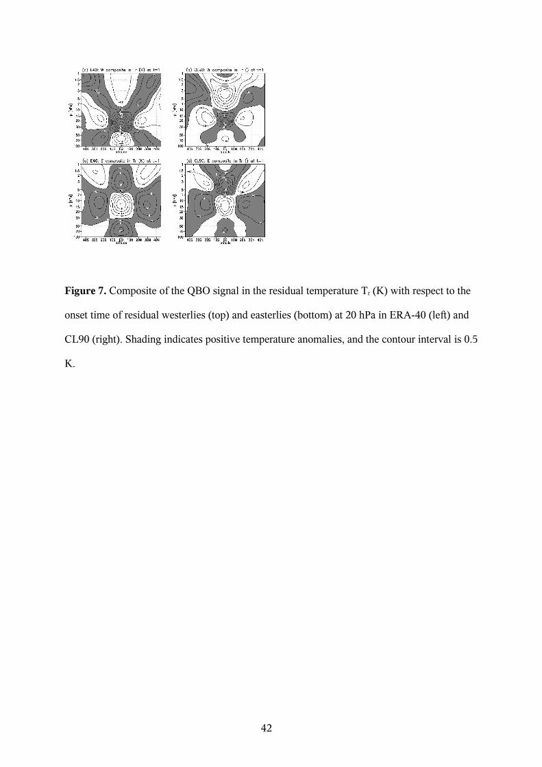
Figure 7. Composite of the QBO signal in the residual temperature Tr (K) with respect to the

onset time of residual westerlies (top) and easterlies (bottom) at 20 hPa in ERA-40 (left) and

CL90 (right). Shading indicates positive temperature anomalies, and the contour interval is 0.5

K.

42

Figure 8. Composites of tendencies ∂U/∂t|∇⋅FEP (top) and ∂U/∂t|GWD (bottom) for westerly

phase (left) and easterly phase (right). Color shading shows tendencies ∂U/∂t in a logarithmic

scale; contours show the composites of the QBO phase in intervals of 5 ms-1.

43

Figure 9. Advective tendencies ∂U/∂t|adv for the composite westerly phase (left) and the

composite easterly phase (right). Color shading shows tendencies ∂U/∂t in a logarithmic scale;

contours show the composites of the QBO phase in intervals of 5 ms-1.

44

Figure 10. Vertical profiles of the QBO (black dashed) and tendencies ∂U/∂t|∇⋅FEP (green),

∂U/∂t|GWD (red), ∂U/∂t|adv (blue) and their sum (black) averaged from 5°N to 5°S for the

composite westerly phase (left) and the composite easterly phase (right).

45

Figure 11. Annual mean tropical upwelling w* (mms-1) in the experiments CL90 (a, solid)

and CL39 (a, dashed). Atmospheric tape recorder signal: Upward propagation of zonal mean

moisture anomalies between 10°N and 10°S in CL90 (b) and CL39 (c). Shading indicates

positive anomalies; contour intervals are 0.1 ppmv. Dashed lines indicate the evolution of the

maxima and minima in the vertical profiles of moisture anomalies.

46

Figure 12. Semi-annual oscillation as seen in the climatological annual cycle of the monthly

zonal mean zonal wind U (ms-1) averaged between 5°S and 5°N in CL90 (a) and CL39 (b).

Shading indicates westerlies; the contour interval is 10 ms-1. Monthly variance Var(U) in m2s-2

(solid), variance of the climatological annual cycle Var(Ucm) (dashed) and the difference Var

(U)-Var(Ucm) (dot-dashed) in CL90 (c) and CL39 (d).

47

Figure 13. Composites of westerly phases in Ur in sensitivity experiments, see also Table 1.

(a) 67-layer vertical grid, (b) 52-layer vertical grid, (c) T31 horizontal truncation, (d) T63

horizontal truncation, (e) 10% reduction in rms-wind, (f) 10% increase in rms-wind. Shading

indicates westerlies, the contour interval is 5 ms-1, and time is shown in units of years.

48