Embed Size (px)
Citation preview

Climate Change and the Chesapeake Bay �
Climate Change and the Chesapeake BayState-of-the-Science Review and Recommendations
A Report from the Chesapeake Bay Program Science and Technical Advisory Committee (STAC)
Coordinating STAC members: Christopher R. Pyke1 and Raymond Najjar2
Contributing authors: Mary Beth Adams3, Denise Breitburg4, Carl Hershner5, Robert Howarth6, Michael Kemp7,
Margaret Mulholland8, Michael Paolisso9, David Secor10, Kevin Sellner11, Denice Wardrop12, and Robert Wood13

Climate Change and the Chesapeake Bay�
1. CTGEnergetics,Inc.,101N.ColumbusSt.,Suite401,Alexandria,VA22314,Tel:202-731-0801,e-mail:[email protected]. DepartmentofMeteorology,ThePennsylvaniaStateUniversity,UniversityPark,PA16802-5013,Tel:814-863-1586,
e-mail:[email protected]. USDAForestService,TimberandWatershedLaboratory,Parsons,WV262874. SmithsonianEnvironmentalResearchCenter,P.O.Box28,Edgewater,MD210375. VirginiaInstituteofMarineScience,Rt.1208,Gr/eateRoad,P.O.Box1346,GloucesterPoint,VA230626. DepartmentofEcologyandEvolutionaryBiology,CornellUniversity,E311CorsonHall,IthacaNY148537. UniversityofMaryland,CenterforEnvironmentalScience,HornPointLaboratory,P.O.Box775,Cambridge,MD216138. DepartmentofOcean,Earth&AtmosphericScience,OldDominionUniversity,4600ElkhornAvenue,Norfolk,VA23529-02769. DepartmentofAnthropology,1111WoodsHall,UniversityofMaryland,CollegePark,MD20742-741510.UniversityofMarylandCenterforEnvironmentalScience,ChesapeakeBiologicalLaboratory,1WilliamSt.,Solomons,MD2068811.ChesapeakeResearchConsortium,645ConteesWharfRoad,P.O.Box28,Edgewater,MD2103712.PennStateCooperativeWetlandsCenter,216WalkerBuilding,UniversityPark,PA1680213.CooperativeOxfordLaboratory,904SouthMorrisStreet,Oxford,MD21654-1323

Climate Change and the Chesapeake Bay �
Climate Change and the Chesapeake BayState-of-the-Science-Review and Recommendations
AnIndependentReportbythe Scientific and Technical Advisory Committee

Climate Change and the Chesapeake Bay�
About the Scientific and Technical Advisory Committee
The Scientific and Technical Advisory Committee (STAC) provides scientific and technical guidance to the Chesapeake Bay Program (CBP) on measures to restore and protect the Chesapeake Bay. As an advisory committee, STAC reports periodically to the Implementation Committee and annually to the Executive Council. Since its creation in December 1984, STAC has worked to enhance scientific communication and outreach throughout the Chesapeake Bay watershed and beyond. STAC provides scientific and technical advice in various ways, including: (1) technical reports and papers, (2) discussion groups, (3) assistance in organizing merit reviews of CBP programs and projects, (4) technical conferences and workshops, and (5) service by STAC members on CBP subcommittees and workgroups. In addition, STAC has mechanisms in place that allow it to hold meetings, workshops, and reviews in rapid response to CBP subcommittee and workgroup requests for scientific and technical input. This capability allows STAC to provide the CBP subcommittees and workgroups with the necessary information and support as specific issues arise in working towards the goals outlined in the Chesapeake2000 agreement. STAC also acts proactively to bring the most recent scientific information to the Bay Program and its partners. For additional information, please visit the STAC website at www.chesapeake.org/stac.
Suggested citation:Pyke, C. R., R. G. Najjar, M. B. Adams, D. Breitburg, M. Kemp, C. Hershner, R. Howarth, M. Mulholland, M. Paolisso, D. Secor, K. Sellner, D. Wardrop, and R. Wood. 2008. Climate Change and the Chesapeake Bay: State-of-the-Science Review and Recommendations. A Report from the Chesapeake Bay Program Science and Technical Advisory Committee (STAC), Annapolis, MD. 59 pp.
STAC Publication #08-004
Publication Date: September 2008
Mention of trade names or commercial products does not constitute endorsement or recommendation for use.
To receive additional copies of this publication, contact the Chesapeake Research Consortium and request the publication by title and number.
CoverphotocourtesyofNOAA
CoverdesignandreportdesignbyNinaFisher
PrintingbyHeritagePrintingandGraphics,Leonardtown,Md.,www.heritageprinting.com
Printedonrecycledpaper
Chesapeake Research Consortium, Inc.645 Contees Wharf RoadEdgewater, MD 21037Tel.: 410-798-1283; 301-261-4500Fax: 410-798-0816www.chesapeake.org

Climate Change and the Chesapeake Bay �
Executive Summary ...........................................................................................................................................................5
Section I: Knowledge Gaps and Research Priorities .....................................................................................7
1. Introduction .....................................................................................................................................................................7
2. Climate Drivers of Change in the Chesapeake Bay.......................................................................................7
3. Monitoring Change .......................................................................................................................................................8
4. Impacts on Chesapeake Bay Program Restoration Strategies ...............................................................8
5. Adaptive Responses to Changing Climatic Conditions ...............................................................................9
6. Next Steps ..................................................................................................................................................................... 10
6.1 Understanding the consequences of climate change .............................................................................................. 10
6.2 Understanding ecosystem processes ....................................................................................................................... 10
6.3 Research coordination and leadership ..................................................................................................................... 10
6.4 Climate Change Action Plan ..................................................................................................................................... 11
Section II: Research Review ...................................................................................................................................... 13
1. Introduction .................................................................................................................................................................. 13
2. Climatic and Hydrologic Processes Affecting the Bay .............................................................................. 13
2.1 Atmospheric composition ......................................................................................................................................... 14
2.2 Water temperature ................................................................................................................................................... 14
2.3 Precipitation ............................................................................................................................................................... 17
2.4 Streamflow ................................................................................................................................................................. 18
2.5 Sea level ...................................................................................................................................................................... 20
2.6 Storms ......................................................................................................................................................................... 21
2.7 Climatic and Hydrologic Processes Summary ......................................................................................................... 22
3. Fluxes of Nutrients and Sediment from the Watershed ......................................................................... 22
3.1 Non-point pollution by sediment and phosphorus ................................................................................................. 22
3.2 Non-point pollution by nitrogen .............................................................................................................................. 23
3.3 Atmospheric deposition of nitrogen ........................................................................................................................ 25
3.4 Freshwater wetlands .................................................................................................................................................. 26
3.5 Point source pollution ............................................................................................................................................... 27
Table of Contents
Climate Change and the Chesapeake Bay�
3.6 Summary of watershed biogeochemistry ................................................................................................................... 27
4. Bay Physical Response ............................................................................................................................................. 28
4.1 Circulation .................................................................................................................................................................. 28
4.2 Salinity ......................................................................................................................................................................... 28
4.3 Suspended sediment .................................................................................................................................................. 28
4.4 Bay physics summary ................................................................................................................................................. 29
5. Living Resources .......................................................................................................................................................... 29
5.1 Food webs, plankton, and biogeochemical processes ............................................................................................. 29
5.�.� Nutrient cycling and plankton productivity ........................................................................................................... 30
5.�.� CO� effects on phytoplankton ............................................................................................................................... 31
5.�.� Temperature effects on plankton .......................................................................................................................... 31
5.�.� Harmful algal blooms and pathogens ................................................................................................................... 32
5.�.5 Dissolved oxygen .................................................................................................................................................. 33
5.2 Submerged aquatic vegetation .................................................................................................................................. 34
5.3 Estuarine wetlands ..................................................................................................................................................... 35
5.4 Fish and shellfish ........................................................................................................................................................ 36
5.4.1 Temperature impacts on fish and shellfish ........................................................................................................... 37
5.4.2 Salinity impacts on fish and shellfish .................................................................................................................... 39
5.4.3 Plankton production impacts on fish and shellfish ................................................................................................ 39
5.4.4 Dissolved oxygen impacts on fish and shellfish ..................................................................................................... 40
5.4.5 Other impacts on fish and shellfish ...................................................................................................................... 40
5.5 Living resources summary ......................................................................................................................................... 40
6. Cultural, Social, and Economic Research ......................................................................................................... 41
6.1 Status of research ...................................................................................................................................................... 41
6.2 Anthropological perspectives ................................................................................................................................... 41
6.3 Natural resource economics .................................................................................................................................... 43
6.4 Adaptive responses .................................................................................................................................................... 43
7. Summary ......................................................................................................................................................................... 45
Acknowledgments ............................................................................................................................................................ 46
References ............................................................................................................................................................................. 47
Coordinating Authors .................................................................................................................................................... 59

Climate Change and the Chesapeake Bay 5
The U.S. EPA’s Chesapeake Bay Program charged the Scientific and Technical Advisory Committee (STAC) with reviewing the current understanding of climate change impacts on the tidal Chesapeake Bay and identifying critical knowledge gaps and research priorities. This report addresses that charge and provides the basis for incorporating climate change considerations into resource management decisions.
Evidence from many laboratory, field, and numerical-modeling studies documents the sensitivity of the Bay’s physical, chemical, and biological processes to climate-related forcings of atmospheric CO2 concentration, sea level, temperature, precipitation, and storm frequency and intensity. Scientists have detected significant warming and sea-level-rise trends during the 20th century in the Chesa-peake Bay. Scenarios for CO2 emissions suggest that the region is likely to experience significant changes in climatic conditions throughout the 21st century. Such shifts include: CO2 concentrations increasing by 50 to 160 percent; relative sea level rising by 0.7 to 1.6 meters; and water temperature increasing by 2° to 6° C. Also likely, though less certain, are increases in precipitation quantity (particularly in winter and spring), precipitation intensity, intensity of tropical and extratropical cyclones (though their frequency may decrease), and sea-level variability. Changes in annual streamflow are highly uncertain, though winter and spring flows will likely increase.
The sensitivity of the Chesapeake Bay to climate suggests that the Bay’s functioning by the end of this century will differ significantly from that observed during the last century. Concurrent changes in human activities — notably urbanization, agriculture, resource management, and ecological restoration — have the potential to either exacerbate or ameliorate the climatically induced shifts. Given the uncertainty in precipitation and streamflow forecasts, the direction of some changes remains unknown. Certain consequences, however, appear likely:
• The mean and variance of sea level will increase, elevating the likelihood of coastal flooding and submer-gence of estuarine wetlands;
• Salinity variability will increase on many time scales due to increases in precipitation intensity, drought, and storminess;
• Warming and higher CO2 concentrations will promote the growth of harmful algae, such as dinoflagellates;
• Warming and greater winter-spring streamflow will increase hypoxia;
• Warming will reduce the prevalence of eelgrass, the Bay’s dominant submerged aquatic vegetation;
• Increases in CO2 may mitigate some of the negative impacts of climate change on wetlands and eelgrass by stimulating photosynthesis;
• Warming will alter interactions among trophic levels, potentially favoring warm-water fish and shellfish species in the Bay.
In addition, climate change will bring about poorly under-stood cultural, social, and economic responses, affecting policies and programs that address climate change.
Importantly, the scenarios considered in this study are not predictions. They are plausible future conditions based on combinations of choices that have yet to be made. The magnitude (and, in some cases, the direction) of impacts associated with climate change depends on the magnitude of CO2 emissions over the next century. The scenarios in this study rest on specific combinations of assumptions about population, economic activity, and fossil fuel use. Lower-emissions scenarios will produce less change in the Bay and moderate impacts on sensitive systems. Time still remains to make choices that result in lower-emission outcomes and reduced effects. All scenarios, however, demonstrate significant changes and current trends point to higher emissions and higher relative impacts. Consequently, climate change represents more than a future threat to the Chesapeake Bay. The Bay Program and its partners can and should assess the implications of changing climatic conditions and ensure that resource protection and restoration strategies remain effective under future conditions. This conclusion supports several general recommendations for the Bay Program and its partners:
Executive Summary

Climate Change and the Chesapeake Bay�
• Understand the implications of climate change for important management decisions and, when possible, the consequences of management decisions for climate change (e.g., CO2 emissions).
• Identify and change policies or management actions that directly or indirectly increase CO2 emissions or exacerbate vulnerability to climate change.
• Ensure that monitoring systems can reliably detect signs of climate change and differentiate these signals from restoration or degradation.
• Take immediate action to develop new approaches that ensure restoration strategies and policies remain effective under changing climatic conditions.
• Assume a leadership role in the development of a comprehensive Baywide Climate Change Action Plan to serve as a road map for mitigating the drivers and preparing for the consequences of climate change.
This report describes the foundation of scientific infor-mation underlying these recommendations. The report begins with a summary of knowledge gaps and their impli-cations for the Bay Program in Section I. Section II offers a detailed review of the relevant scientific literature and research. The report concludes with the recommendation to develop and implement a research coordination and support program that addresses the critical issues raised throughout the document.

Climate Change and the Chesapeake Bay �
– 1 –Introduction
The Earth’s climate is changing due to human activities. Global temperatures have risen by more than 0.5° C over the last century and models suggest far-reaching changes in climate over the next century [IPCC, 2007]. The United Nation’s Intergovernmental Panel on Climate Change (IPCC) has repeatedly evaluated the consequences of these changes and found the potential for severe impacts on human health, ecosystems, water resources, and agricul-tural systems. The Chesapeake Bay research community is also evaluating the causes and consequences of climate change. As Section II of this report details, higher CO2 concentrations, rising sea level, increasing temperatures, and changes in precipitation and storminess are likely to have significant consequences for both the Chesapeake Bay ecosystem and the Chesapeake Bay Program’s goals for water quality and living resources restoration (as described in the Chesapeake2000agreement).
This review focuses on four research themes directly relevant to the Chesapeake Bay Program:
• Climatic drivers of change;
• Monitoring of changing conditions;
• Impacts of changing climate on restoration strategies and Bay Program goals; and
• Development of resilient and adaptive management strategies.
These themes are interrelated; however, they are not fungible. Effort directed towards one issue cannot substitute for attention to the others. Similarly, priorities set in one area should not take precedence over priorities in other areas. All these equally important elements are required to understand and address climate change in the Chesapeake Bay. Effective action mandates adequate consideration of each area; conversely, inattention to any category undermines the value of work in all of them.
Section I of this report provides a set of conclusions, observations, and recommendations based on an extensive review of the scientific research presented in Section II. The
report also presents three types of prospective research questions for each theme:
• One critical question associated with each research area, with the success of the Bay Program depending on immediate efforts to address this question.
• Two to four additional important questions presented after each critical question, representing the next tier of issues with near-term implications.
• Several additional relevant technical questions throughout Section II that reflect gaps in current scien-tific understanding and opportunities for productive lines of future research.
– 2 –Climate Drivers of Change
in the Chesapeake BayClimate variability and climate change create significant challenges for the restoration of water quality and living resources in the Chesapeake Bay. Understanding the spatial and temporal dynamics associated with the processes driving the physical system (physical drivers) is essential for developing effective responses to these challenges. Researchers have also identified physical changes in the system through analysis of historic observations and climate system modeling, including past and projected changes in atmospheric CO2 concentration, sea level, temperature, precipitation, streamflow, and storms (Section II.2).
Trends and scenarios for sea level and temperature are relatively well constrained. There is more uncertainty regarding future precipitation regimes — perhaps the most important variable in understanding the future of the Chesapeake Bay. Spatial and temporal changes in precipi-tation patterns have far-reaching implications for the Bay through their direct and indirect impacts on watershed hydrology (Section II.2.4) and essential biogeochemical processes (Section II.3 and Section II.5.1). Higher air temperature and concurrent stressors, such as land cover change, would likely exacerbate these impacts. Developing a more comprehensive and sophisticated understanding
Section IKnowledge Gaps and Research Priorities

Climate Change and the Chesapeake Bay�
of the possible changes in regional precipitation and the implications of potentially unprecedented combinations of temperature and precipitation is essential.
– 3 –Monitoring Change
Environmental monitoring remains an essential component of the Chesapeake Bay Program. Computer models and simulations help develop environmental policy and regulation, but the ultimate success (or failure) of the program rests on real-world conditions. Climate change compounds the already critical need for monitoring, but also creates new challenges. The design of Chesapeake Bay monitoring systems must allow detection of long-term trends andallow managers to differentiate climate-driven changes from those associated with restoration actions or other sources of degradation. These distinctions are essential for understanding the efficacy of management efforts and determining the causes of change in ecosystem health and water quality. The Bay Program must evaluate the consequences of climate change for existing monitoring systems and ensure that sampling designs provide adequate statistical power to detect trends and differentiate sources of improvement or degradation.
– 4 –Impacts on Chesapeake Bay
Program Restoration StrategiesUnderstanding of the physical drivers of change and consideration for the effectiveness of environmental monitoring ultimately create a solid foundation for asking the most important question facing the Bay Program: WhataretheimplicationsofclimatechangefortheBayProgram’seffortstorestorewaterqualityandlivingresources?
Three of the Bay Program’s most important approaches for Chesapeake restoration are:
• Baywide water quality regulation (e.g., Total Maximum Daily Loads — TMDLs);
• State tributary strategies to achieve the goals of the Chesapeake2000 agreement; and
• Activities to protect and restore living resources (e.g., submerged aquatic vegetation (SAV), oysters, and fisheries).
These strategies are central to the success of the Bay Program and all are sensitive to climate. Climate change, therefore, is likely to undermine key assumptions in the current approaches used to develop and deploy these strategies. For example, calculations for estimating
Critical Climatic Drivers of Change Question:
How will climate change alter regional precipitation patterns and what are the most important aspects of precipitation change for ecosystem and watershed processess?
Important Questions:
• What is the relationship between river flow and regional air temperature? How might this relationship change under future climatic conditions?
• Can existing watershed models (e.g., the CBP Phase V model) accurately simulate runoff and river flow regimes under plausible future combinations of precipitation and temperature?
• How will climate-driven changes interact with concurrent changes, such as land use/land cover shifts, invasive species, and social and economic processes, to alter the physical environment (e.g., the timing and magnitude of stormwater runoff)?
Critical Monitoring Question:
How should a Baywide monitoring system be designed, deployed, and operated to detect and differentiate climate-driven changes from other sources of change?
Important Questions:
• Can the existing monitoring system provide the statistical power needed to detect trends reliably in the climatic variables associated with key management decisions, including peak water temperatures, summer wind regimes, as well as the frequency and severity of droughts?
• Which environmental measures provide the most sensitive indicators of climate change?
• Which environmental indicators are relatively insensitive to climate change?
• How can information about the relative sensitivity of physical, chemical, and biological indicators be conveyed to policymakers, managers, and other stakeholders to inform resource management?

Climate Change and the Chesapeake Bay �
quite sensitive to peak summer temperatures and flow regimes (Section II.5.2). Climate change will likely alter both variables and likely hinder restoration success. Fortu-nately, identifying these climatic assumptions is possible in developing more sustainable restoration plans. Experience in other ecosystems has shown that it is possible, for example, to identify resilient sites where cool local waters offset rising regional temperatures and sustain restored populations. The Bay Program and its partners should assess the vulnerability of living resource restoration efforts to climate change and require that projects take specific steps to increase the likelihood of success under changing conditions.
Each of these cases illustrates that climate change can directly affect key Chesaeake Bay Program strategies. The program must consider these impacts in more detail, and, most importantly, explicitly incorporate information on changing climatic conditions into analyses and decision-making.
– 5 –Adaptive Responses to
Changing Climatic Conditions
Understanding the impact of climate change on Bay Program priorities sets a foundation for changes in management practice that anticipate and respond to shifting conditions. The climate-change-science community calls such responses “adaptation.” Although adaptation is a long-standing area of scientific research, interest has increased in recent years as resource managers noticed early signs of climate change and recognized that additional impacts are likely and, quite possibly, inevitable.
Researchers distinguish between resilient and adaptive responses to climate change impacts. Resilient responses increase the capacity of a human or ecological system to respond to disturbance and accommodate changing condi-tions. Such responses typically do not require assumptions or forecasts about future conditions, but rather identify opportunities to make decisions more robust to a range of future conditions (e.g., as in the case of poorly constrained precipitation forecasts in Section II.2.3). Adaptiveresponses go further by basing management on both current obser-vations and anticipated future conditions. Adaptive approaches are particularly appropriate for decisions dealing with situations in which rising sea levels and temperatures demonstrate clear trends and consistent projections (Sections II.2.2 and II.2.5).
TMDLs are based on a carefully selected subset of historic meteorological observations. Trends in variables, such as temperature or precipitation, violate assumptions used in these calculations and, therefore, undermine confidence in the results. The Bay Program must develop methods to calculate TMDLs that explicitly incorporate information about changing climatic conditions.
State partners have developed restoration and resource protection plans known as tributary strategies. These plans describe the combinations of approaches needed to restore Bay water quality. The effectiveness of individual management practices is central to the design of tributary strategies. The understanding of their performance rests on observations under historic climatic conditions. For example, the ability of retention ponds to capture sediment and remove nutrients varies with precipitation volume and intensity along with other climatic factors. Practices based on historic precipitation regimes may not meet performance goals under future conditions. Similar considerations apply to most of the 58 individual best management practices (BMPs) in the state tributary strategies. The Bay Program and its partners must assess the consequences of climate change for the efficacy of management practices.
Similar considerations also apply to living resources. Restoration efforts rely on understanding historic relation-ships between climatic conditions and ecological processes. Climatic shifts, however, are likely to jeopardize these relationships. For example, the Bay Program places great weight on planting SAV. Some SAV species, however, are
Critical Restoration Strategy Question:
How will state tributary strategies and living resource restoration strategies perform under changing climatic conditions?
Important Questions:
• How will climate change alter the cost or feasibility of achieving water quality and living resource restoration goals?
• What are the implications of sea-level rise for tidal wetland loss, shoreline and nearshore erosion, inundation of low-lying coastal communities, and shoreline hardening strategies?
• What are the implications of climate change for non-indigenous species, diseases, pathogens, and pests?

Climate Change and the Chesapeake Bay�0
In these situations, basing decisions with long-term consequences on historic observations alone would prove irresponsible. Simply planning for a very broad range of future conditions (i.e., “super-sized” infrastructure), however, is usually inefficient. Resource managers must anticipate future conditions and design accordingly.
As with any adaptive approach, effective and efficient action requires close coupling of management and monitoring to understand, prepare for, and respond to changing conditions. The Bay Program and its partners can and should increase the resilience of its activities to uncertain precipitation regimes and adapt them to rising temperatures and sea levels.
– 6 –Next Steps
Climate change represents more than a future threat to the Chesapeake Bay. The Bay Program and its partners are making far-reaching decisions with implications that extend decades into the future. In this context, climate change demands immediate consideration in efforts to protect and restore water quality and living resources. The Bay Program and its partners must take immediate action to understand the consequences of changing climatic conditions and make consideration of climate change an integral part of decision-making.
6.1 Understanding the consequences of climate change
The Bay Program and its partners should address these issues through its current authorities, responsibilities, and resources. The first — and perhaps most important — step is to explicitly consider climate change in a wide range of resource management decisions: water quality regulation, tributary strategies, living resource restoration, and others. These decisions typically are based on historic climatic observations and likely are quite sensitive to climate change. The Bay Program and its partners can and should immediately require all major resource management decisions to evaluate changing conditions on both the cost and efficacy of the action and explicitly consider management options that increase resilience or facilitate adaptation to changing conditions.
6.2 Understanding ecosystem processes
The uncertainties of climate change on ecosystem processes pose significant challenges for The Bay Program. Some of the most pressing issues include:
• The implications of climate change for precipitation and evapotranspiration, particularly the representa-tion of these processes in the Phase V watershed model (Sections II.2.3 and II.2.4).
• The impact of climate change on non-point source loadings (Sections II.3.1 and II.3.2).
• The role of food web dynamics in mediating the response of estuarine ecosystems to changing conditions (Section II.5).
• The consequences of climate change for specific targets, such as harmful algal blooms, the biogeography of disease, and fisheries productivity (Sections II.5.1.4 and II.5.4)
Efforts to address these issues will require acceleration and reorientation of existing lines of research. In some cases, it may create new motivations to address long-standing ecological issues, such as Bay food web dynamics. The Bay Program and its partners can and should provide direct support and, when possible, encourage research sponsors to provide targeted resources for climate-change-related research on key ecosystem processes.
6.3 Research coordination and leadership
With notable exceptions, the current body of knowledge reflects a history of relatively broad-based, short-term research. This situation arose from decades of sporadic
Critical Climate Adaption Question:
How can restoration strategies be designed, deployed, and monitored to ensure that they are resilient and adaptive to changing climatic conditions?
Important Questions:
• How can water quality regulations be made resilient to climatic fluctuations and anticipate changing climatic conditions?
• How can ecological restoration strategies antici-pate rising sea levels and changing temperature regimes?
• How should management practices be altered to increase their resilience to future precipitation regimes?
• How can coastal landowners make resilient and, when possible, adaptive decisions about their responses to rising sea levels?
Climate Change and the Chesapeake Bay ��
funding, a lack of institutional commitments, and the absence of widely-recognized research priorities. No institutional focal point for climate change research and development activities relevant to the Chesapeake Bay currently exists.
This situation contrasts with several regions that have strong, long-standing relationships intertwining climate science, public policy, and ecosystem restoration. For example, the Climate Impacts Group (CIG) at the University of Washington is an award-winning interdis-ciplinary research group that researches natural climate variability and global change to increase the resilience of the Pacific Northwest to fluctuations in climate. The CIG has contributed demonstrably to a foundation of knowledge that supports some of the most progressive climate change policy in the nation (e.g., King County, Washington’s 2007 Climate Plan). The Chesapeake Bay would benefit greatly from a similar organization. The Bay Program and its partners should take the lead in estab-lishing an organization that links climate science, policy, and management throughout the watershed as quickly as possible.
6.4 Climate Change Action Plan
An assessment of climatic assumptions and sensitivities offers immediate opportunities for improvement to internal Bay Program decision-making processes. This step is necessary but insufficient to address the scope of the problem. Equally important, the Bay Program must take a leadership role in addressing climate change across the watershed. One mechanism for adopting this role is through development of a multi-jurisdictional, Bay-focused Climate Change Action Plan.
This plan would build on and complement state-level climate action plans, emphasizing impacts and adaptation opportunities for the protection and restoration of the Chesapeake Bay. The plan should include a detailed road map for research and management to assist the Bay Program in achieving its mission in a changing climate. The Baywide Climate Change Action Plan would also provide a focal point for identifying and coordinating policies, regulations, and strategies that contribute directly or indirectly to drivers of climate change. The Bay Program and its partners should take immediate action to promote and support the development of a Baywide Climate Change Action Plan.

Climate Change and the Chesapeake Bay��

Climate Change and the Chesapeake Bay ��
– 1 –Introduction
This section offers an up-to-date review of research dealing with climate change impacts on the Chesapeake Bay. This review does not cover the full depth of current understanding, but surveys the breadth of relevant work. The section follows a logical progression from changes in the physical conditions that affect the Chesapeake to their impacts on water quality and living resources and ending with current opportunities for adaptive management actions.
We limited the scope of the review to climate change impacts and adaptive management strategies, excluding mitigation activities such as the regulation of climate change drivers (most notably greenhouse gas emissions). We strongly believe that greenhouse gas mitigation remains essential for solving climate change problems in the Chesapeake Bay and other estuaries. The magnitude and, in some cases, the direction of climate change impacts depend on quantities of CO2 emissions over the next century.
The scenarios in this study rest on combinations of assumptions about population, economic activity, and fossil fuel use. Lower-emissions scenarios will produce less change in the Bay and reduce impacts on sensitive systems. Time still remains to make the choices that lead to lower emissions and reduced impacts. All scenarios, however, point to significant change with current trends suggesting higher emissions and greater relative impacts.
The Bay Program may play a role in reducing emissions, particularly when its interests overlap with land use, agriculture, transportation, and infrastructure. Consideration of these issues remains important, but rests beyond the scope of this study. These issues require and deserve an independent investigation.
We also limited the scope of the review to the tidal Chesapeake Bay, excluding terrestrial and freshwater impacts other than those that also affect tidal areas of the basin. Several recent reviews consider terrestrial impacts in
and around the Chesapeake watershed [Abler et al., 2002; Iverson et al., 2008; Moore et al., 1997; Ollinger et al., 2008; Paradis et al., 2008; Rodenhouse et al., 2008; Rogers and McCarty, 2000; Wolfe et al., 2008]
Many of the activities and products in the following sections are associated with a series of important research efforts, including:
• Mid-Atlantic Regional Assessment (MARA), 1998 – 2000, funded by the Environmental Protection Agency
• Consortium for Atlantic Regional Assessment (CARA), 2003 – 2006, funded by the Environmental Protection Agency
• Northeast Climate Impacts Assessment (NECIA), ongoing, organized by the Union of Concerned Scientists
• Coastal Hypoxia Research Program (CHRP), ongoing, funded by the National Oceanic and Atmospheric Administration.
This report builds directly on several important earlier reviews, including those that focused on the impact of climate change on ecosystems, coastal areas, and marine resources of the Mid-Atlantic region [Moore et al., 1997; Moss et al., 2002; Najjar et al., 2000; Rogers and McCarty, 2000; Wood et al., 2002], the United States [Field and Boesch, 2000; Scavia et al., 2002], and the world [Kennedy et al., 2002].
– 2 – Climatic and Hydrologic Processes
Affecting the BayClimate change can influence estuaries — which interface with the land, atmosphere, and open ocean — in various ways, including:
• The direct effect of changing atmospheric composition on the chemistry of the estuary;
• Changes in water temperature;
• Changes in freshwater inflow quantity and quality due to climatic shifts in the watershed (mainly precipitation and temperature); and
Section IIResearch Review
Climate Change and the Chesapeake Bay��
decade. Figure 2 also shows an estimate of surface water temperature averaged over the mainstem Bay based on data from the Chesapeake Bay Water Quality Monitoring Program, which has sampled the water column at least monthly at several dozen stations throughout the mainstem Bay since 1984. The correspondence between the pier and the Bay-average data during the period of overlap indicates that the longer time series measured at the piers reflect mean Bay temperature quite well.
Austin [2002] noted a correspondence of York River surface water temperature with the North Atlantic Oscillation (NAO) index, particularly when averaging the data over several years (correlations of annually averaged quantities were much lower). He also determined that the beginning of spring (defined by the date when water temperature first reaches 15° C — a critical temperature when many Bay species spawn or migrate) occurred roughly three weeks earlier in the 1990s compared to the 1960s. Analyzing the same York River water temperature time series, Wood et al.[2002] found significant warming trends in seven of the 12 calendar months within the spring, summer, and winter seasons. Preston [2004] analyzed surface (≤ 1 m) and subsurface (≥ 15 m) temperature data from the Chesapeake Bay Water Quality Monitoring Program (1984 – 2002), as well as historical data archived by the Chesapeake Biological Institute (from 1949). Annual water temperature anomalies were positively and significantly correlated (p < 0.05, Bonferroni adjusted t-test) with regional air temperature as well as Northern Hemisphere mean air temperature, suggesting large-scale controls on Bay water temperature. This finding is consistent with Austin’s [2002] connection of Bay temperature with the North Atlantic Oscillation (NAO) and Cronin et al.’s[2003] detection of strong correspondence between temperature anomalies in the Bay and on the continental shelf at monthly to inter-
• Changes in forcing from the open ocean, including sea-level rise.
This section discusses observed trends and future projec-tions of atmospheric CO2, temperature, precipitation, streamflow, and sea level in the Bay region. Section II.3 covers changes in the quality of freshwater inputs.
2.1 Atmospheric composition
Atmospheric CO2 is well mixed, making regional and global projections of this gas essentially identical. Projec-tions for global mean atmospheric CO2 concentration over the next 100 years vary widely. This variation results primarily from uncertainty in future CO2 emissions (Figure 1), but also from unknown feedback links between climate and the carbon cycle and differences in the representation of Earth system processes in simulation models.
The relatively short equilibration time of CO2 at the air-sea interface (about 1 year) suggests that changes in surface-water CO2 should closely track those of atmospheric CO2. This relationship will likely result in a decrease of both the pH and carbonate ion concentration 2
3[CO ]− (determined from the chemical equilibria of the carbonate system). CaCO3-secreting organisms (such as many shellfish) require 2
3[CO ]− to occur above a certain level — typically the saturation concentration — making 2
3CO − of particular interest. Orr et al. [2005] showed that average 2
3[CO ]− and pH decreases of about 10% and 0.1, respectively, have already occurred throughout the surface ocean due to invasion of anthropogenic CO2. Under a greenhouse gas scenario similar to the Intergovernmental Panel on Climate Change’s SRES A2 storyline (Figure 1 and box on page 16), these changes increase to 45% and 0.5, respectively, by 2100. We are not aware of similar studies in estuaries, where the salinity, alkalinity, and dissolved inorganic carbon (which influence the sensitivity of pH and 2
3[CO ]− to CO2) may differ dramatically from their seawater counterparts.
2.2 Water temperature
Figure 2 shows 20th-century surface water temperature variability at two piers in the Chesapeake Bay — one near the mouth of the York River located 45 km from the Chesapeake Bay mouth [Austin, 2002] and the other near the mouth of the Patuxent River, which empties into the central portion of the Bay [Secor and Wingate, 2008]. Although highly variable, the measurements indicate long-term warming. The 1990s were about 1° C warmer than the 1960s, suggesting a warming trend of about 0.3° C per
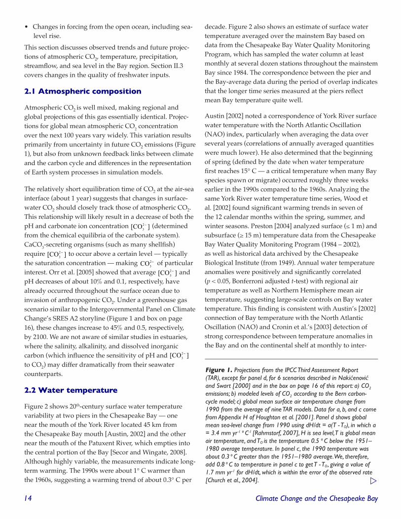
Figure 1. Projections from the IPCC Third Assessment Report (TAR), except for panel d, for � scenarios described in Nakićenović and Swart [�000] and in the box on page �� of this report: a) CO�
emissions; b) modeled levels of CO� according to the Bern carbon-cycle model; c) global mean surface air temperature change from ���0 from the average of nine TAR models. Data for a, b, and c come from Appendix H of Houghton et al. [�00�]. Panel d shows global mean sea-level change from ���0 using dH/dt = a(T - TO), in which a = �.� mm yr-� o C-� [Rahmstorf, �00�], H is sea level, T is global mean air temperature, and TO is the temperature 0.5 o C below the ��5�–���0 average temperature. In panel c, the ���0 temperature was about 0.� o C greater than the ��5�–���0 average. We, therefore, add 0.� o C to temperature in panel c to get T - TO, giving a value of �.� mm yr-� for dH/dt, which is within the error of the observed rate [Church et al., �00�]. w

Climate Change and the Chesapeake Bay �5
Te
mp
era
ture
Ch
an
ge (
o C
)S
ea
Le
vel
Ch
an
ge (
mm
)C
O2 (
pp
m)
Em
issi
on
s (P
g C
y-1
)

Climate Change and the Chesapeake Bay��
annual time scales since the 1980s. Cronin et al.[2003] also documented several rapid shifts of Chesapeake Bay spring temperature of ~2 – 4° C over the past two millennia. Mean spring water temperature was 1.6 to 2.4° C higher during the 20th century than from 1720 to 1850.
Taken together, the temperature studies show a strong correlation between water temperature in the Bay and regional atmospheric and oceanic temperatures at monthly to decadal time scales. Thus, regional temperature projections from climate models likely can be applied directly to the Bay. Such an application is fortunate since
climate models (even nested regional climate models) do not have a spatial resolution sufficiently fine to depict the Chesapeake Bay.
Two recent studies analyzed the output of global climate models (GCMs) in the Chesapeake Bay region. As part of CARA, Najjar et al. [2008] scrutinized the output of seven GCMs over three major mid-Atlantic estuaries (Chesa-peake Bay, Delaware Bay, and the Hudson River Estuary). Projections differ greatly among the models (Figure 3), but historically the multi-model average generally performs better than individual models. The multi-model average
IPCC Climate Change Scenarios
The United Nation’s Intergovernmental Panel on Climate Change (IPCC) has developed a set of socioeconomic scenarios as the basis for climate change modeling and policy analysis. The following verbatim descriptions from Nakicenovic and Swart [2000] are the most widely used scenarios:
A1 Future world of very rapid economic growth, global population that peaks in the mid-21st century and declines thereafter, and the rapid introduction of new and more efficient technologies. Major
underlying themes are convergence among regions, capacity building, and increased cultural and social interactions, with a substantial reduction in regional differences in per capita income. The A1 scenario family has three groups that describe alternative directions of technological change in the energy system: fossil intensive (A1FI), non-fossil energy sources (A1T), or a balance across all sources (A1B) (where balanced is defined as not relying too heavily on one particular energy source, on the assumption that similar improvement rates apply to all energy supply and end use technologies).
A2 A very heterogeneous world where the underlying theme is self-reliance and preservation of local identities. Fertility patterns across regions converge very slowly, which results in continuously
increasing population. Economic development is primarily regionally oriented and per capita economic growth and technological change are more fragmented and slower than other storylines.
B1 A convergent world with the same global population, that peaks in mid-century and declines thereafter, as in the A1 storyline, but with rapid change in economic structures toward a service and
information economy, with reductions in material intensity and the introduction of clean and resource-efficient technologies. The emphasis is on global solutions to economic, social, and environmental sustainability, including improved equity, but without additional climate initiatives.
B2 A world in which the emphasis is on local solutions to economic, social, and environmental sustainability. It is a world with continuously increasing global population, at a rate lower than A2, and
with intermediate levels of economic development, and less rapid and more diverse technological change than in the B1 and A1 storylines. While the scenario is oriented toward environmental protection and social equity, it focuses on local and regional levels.
When considering future conditions in the Chesapeake Bay, it is important to note that no direct connection exists between these global storylines and regional conditions. This situation makes it important to consider carefully the implied relationship between global drivers and local and regional conditions (e.g., population size, technology choices, etc.). The U.S. EPA Global Change Research Program is currently developing tools to provide national and regional realizations of IPCC storylines for urban land cover through their Integrated Climate and Land Use Scenarios (ICLUS) project.

Climate Change and the Chesapeake Bay ��
could track the observed 20th-century warming of the northern watersheds (Hudson, Delaware, and Susque-hanna River), but not the weak cooling in the southern portion of the Chesapeake watershed [e.g., Allard and Keim, 2007]. The multi-model average also simulated the long-term annual average temperature well, but overes-timated the annual temperature range (summer minus winter) and interannual variability. Model-averaged projec-tions for the six scenarios in Figure 1 range from 3 to 6° C of warming by 2070 to 2099 (Figure 4a). With use of the best-performing models, the projected change decreases to 2 to 5° C of warming (Figure 4b).
In the second study, Hayhoe et al. [2007] conducted an analysis under NECIA of nine global climate models for the northeast United States (Pennsylvania to Maine), which includes the northern half of the Bay watershed (essentially the Susquehanna River basin). They found that the multi-model average captures the observed long-term increase in annual-mean regional air temperature during the 20th century, including the acceleration over the last 30 years. Projected temperature changes were similar to those of Najjar et al. [2008].
Shifts in temperature extremes are as important as annual mean temperature changes (noted below for submerged aquatic vegetation in Section II.5.2). Meehl et al. [2007] analyzed the output of nine global climate models for changes in heat waves, defined as “the longest period in the year of at least five consecutive days with maximum temperature at least 5° C higher than the climatology of the same calendar day.” Under the A1B scenario, heat waves along the East Coast of North America, including the Mid-Atlantic, are projected to increase by more than two standard deviations by the end of the 21st century.
2.3 Precipitation
Though precipitation falling directly on the Chesapeake has a very small influence on its overall water balance, precipitation falling on its watershed is extremely important in regulating streamflow entering the Bay. This freshwater inflow is a dominant driver of Bay circulation, biogeochemistry, and ecology. Several studies document 20th-century increases of precipitation in the United States, including the Northeast, particularly in extreme wet events [Groisman et al., 2001; Groisman et al., 2004]. Climate models have, in general, been unable to simulate this long-term change in precipitation in the northeast United States [Hayhoe et al., 2007; Najjar et al., 2008]. Climate models do capture long-term means of annual, winter, and
summer precipitation over the Chesapeake Bay watershed, though with a tendency to predict too much precipitation in spring and too little in fall [Najjar et al., 2008]. Hayhoe et al. [2007] and Najjar et al. [2008] showed similar results regarding GCM precipitation predictions under enhanced greenhouse gas levels:
• Multi-model averages of more annual precipitation (Figures 4c and 4d);
• A broad spread among models of annual precipitation change (Figure 3); and
• Greater consensus among the models in winter and spring, when precipitation is projected to increase (Figure 3).
For example, over the Chesapeake Bay watershed, precipitation changes over the 21st century range from -17% to +19% (multi-model mean of 3%) under the A2 scenario [Najjar et al., 2008]. In winter, the model range is -5% to +16% (multi-model mean of 8%). The broad spread in modeled precipitation changes reflects the Mid-Atlantic region’s location at the boundary separating subtropical precipitation decreases and subpolar precipi-tation increases; consensus increases for the winter as this boundary moves south [Meehl et al., 2007].
One important characteristic of precipitation is intensity, particularly for watershed export of sediment, phosphorus, and (to a lesser extent) nitrogen to estuaries (Sections II.3.1 and II.3.2). Defining intensity as the annual
Figure 2. Annual average surface temperature from the mouth of the York River (VIMS pier), the mouth of the Patuxent River (CBL pier), and the average throughout the mainstem Bay (Bay average). The VIMS data come from Austin (�00�) and the CBL data come from Secor and Wingate (�00�). The VIMS data are part of the VIMS Scientific Data Archive, acquired from Gary Anderson at VIMS. David Jasinski, Chesapeake Bay Program Office, computed the Bay-average data using measurements from the Chesapeake Bay Water Quality Monitoring Program. Data were first averaged by month at each station, then by year, before taking the arithmetic mean of all stations.

Climate Change and the Chesapeake Bay��
mean precipitation divided by the number of days with rain, Meehl et al. [2007] showed that many models predict significant increases of this variable, particularly at middle and high latitudes (including the Mid-Atlantic region). Under the A1B scenario, mid-Atlantic precipitation intensity is expected to increase by one standard deviation by the end of the 21st century. The increase in precipitation intensity resulted from the increase in annual precipitation as well as the number of dry days — a finding consistent with changes in storm frequency and intensity (Section II.2.6).
2.4 Streamflow
Streamflow reaching the Bay is governed by how much precipitation falls on its watershed, but also by evapo-transpiration loss to the atmosphere and watershed storage changes. Over interannual time scales, storage changes are believed small; thus, streamflow simply equals the excess of precipitation over evapotranspiration averaged over the watershed. Averaged over many years, streamflow
to the Bay is about 40% of precipitation throughout the watershed [Sankarasubramanian and Vogel, 2003].
Much of the interannual variability in streamflow to the Bay is driven by precipitation, with a relatively small role for evapotranspiration. Najjar [1999], for example, found that watershed precipitation explains 89% of the variability of annual-average Susquehanna River flow (half the total freshwater flow to the Bay). Austin [2002] examined the 1957 to 2000 record of annual streamflow into the Chesapeake and found substantial interannual variability (a range of more than 2.5) as well as decadal variability characterized by dry conditions during the 1960s, wet conditions during the 1970s, and relatively normal condi-tions since then. He noted no obvious long-term trend, though others [Groisman et al., 2001; Groisman et al., 2004] characterize the Northeast as a region of increasing streamflow, particularly in extreme wet events. Saenger et al. [2006] provided a longer-term perspective on flow into the Bay using salinity proxy data and streamflow-salinity relationships to infer variability in Susquehanna River
Figure 3. Seasonal temperature (top) and precipitation (bottom) changes averaged over the Chesapeake Bay watershed with respect to ���� to �000 predicted under the A� scenario by seven climate models for �0�0 – �0��, �0�0 – �0��, and �0�0 – �0��. At the far right of each panel are the annual average changes for the seven-model mean and the overall model range (reproduced from Najjar et al. [�00�]).

Climate Change and the Chesapeake Bay ��
Figure 4. Projected change in the annual mean temperature (a and b) and precipitation (c and d) of the Chesapeake Bay watershed for six IPCC scenarios (see Figure �) averaged over seven climate models (a and c) and the four highest ranked (b and d). From Najjar et al. [�00�].
flow throughout the Holocene. Their analysis suggests that average streamflow 6000 to 7000 years ago was 72% lower than during the past 1500 years. Large decadal and centennial variability during the last 1500 years was also inferred.
Previous hydrological modeling studies find widely varying streamflow projections in the northeast United States (Table 1), even when forced by the same climate models [Neff et al., 2000; Wolock and McCabe, 1999]. This result is puzzling, especially given that hydrological models generally are able to hindcast the historical streamflow record in the Mid-Atlantic region accurately [e.g., Hayhoe et al., 2007; Najjar, 1999; Swaney et al., 1996; Wolock et al., 1996]. Most of the past variability, however, is due to changes in precipitation.
The discrepancy in future projections most likely arises because models predict different evapotranspiration responses (and, therefore, streamflow responses) to temperature change. This divergence is probably due to the lack of an observational record of substantial temperature change with which to constrain hydrological
models. For example, the standard deviation of annual air temperature over the Chesapeake watershed is 0.5° C [Najjar et al., 2008] — small compared to the multi-model mean projected 100-year warming (Figure 4). Other confounding influences on streamflow, which are generally not considered in future projections, include vegetation changes, the direct influence of CO2 on evapotranspiration, and land use change (predominantly urbanization, agriculture, and forestry).
The seasonality of streamflow into the Bay is extremely important because it helps regulate timing of the spring bloom (Section II.5.1.1). Hydrological model simula-tions by Hayhoe et al. [2007] in the northeast United States predicted greater wintertime flows (due to snow melt) and depressed summer flows (due to increased evapotranspiration). They also predicted an advance of the spring streamflow peak by nearly two weeks. A statistical approach by Schoen et al. [2007], combined with climate model output, suggested that the 7Q10 (the lowest streamflow for seven consecutive days that occurs, on average, once every 10 years) will decrease substantially in the future.
Climate Change and the Chesapeake Bay�0
Reference Region CO2 Scenario
Time Period
Number of GCMs
Annual StreamflowChange (%)
McCabe and Ayers (1989)
Delaware River Basin Doubling – 3 - 39 to 9
Moore et al. (1989) Mid-Atlantic/New England Doubling – 4 - 32 to 6
Najjar (1999) Susquehanna River Basin Doubling – 2 24 ± 13
Neff et al. (2000) Susquehanna River Basin 1% yr -1 increase
1985 – 1994 to
2090 – 2099
2 - 4 to 24
Wolock and McCabe (1999)
Mid-Atlantic 1% yr -1 increase
1985 – 1994 to
2090 – 20992 - 25 to 33
Hayhoe et al. (2007) Pennsylvania/New JerseyA1F1 and B1 1961 – 1990
to 2070 – 2099
2 9 to 18
Early water balance studies of the Susquehanna River basin also suggested greater winter flows but with less agreement on summer flows and timing of the spring freshet [Najjar, 1999; Neff et al., 2000]. January-to-May average flow of the Susquehanna has been used to predict summertime circulation parameters [Hagy, 2002] and dissolved oxygen levels [Hagy et al., 2004]. Historically, a
strong correlation exists between January-to-May flow and precipitation in this basin such that the percent increase in flow equals the percent increase in precipitation [Najjar, 2008]. Given the consensus among models for rise in spring and winter precipitation, the January-to-May flow of the Susquehanna will likely increase in the future.
Due to the greater number of precipitation-free days as well as the greater evapotranspiration (resulting from higher temperatures), drought will likely increase in the future. Defining drought as a 10%-or-more deficit of monthly soil moisture relative to the climatological mean, Hayhoe et al. [2007] simulated increases in droughts of different durations over the northeast United States. The number of short-term (1 to 3 months) droughts, for example, was projected to increase 24 to 79% (B1 and A1FI scenarios) by 2070 to 2099 compared to 1961 to 1990. Medium (3 to 6 months) and long (over 6 months) droughts had even larger fractional increases. More droughts would affect the functioning of terrestrial ecosystems (particularly wetlands) in the Bay watershed. Greater drought frequency may also mean more frequent saltwater intrusion events into the Chesapeake.
2.5 Sea level
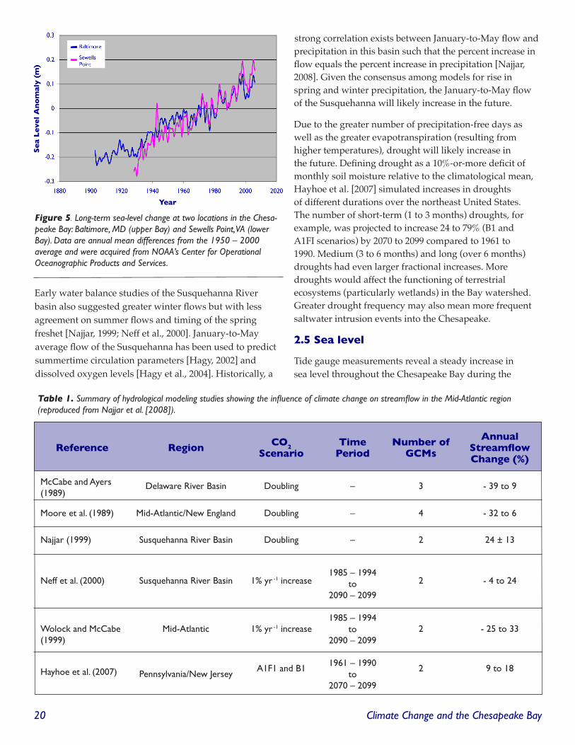
Tide gauge measurements reveal a steady increase in sea level throughout the Chesapeake Bay during the
Figure 5. Long-term sea-level change at two locations in the Chesa-peake Bay: Baltimore, MD (upper Bay) and Sewells Point, VA (lower Bay). Data are annual mean differences from the ��50 – �000 average and were acquired from NOAA’s Center for Operational Oceanographic Products and Services.
Se
a L
eve
l A
no
mal
y (
m)
Year
Table 1. Summary of hydrological modeling studies showing the influence of climate change on streamflow in the Mid-Atlantic region (reproduced from Najjar et al. [�00�]).

Climate Change and the Chesapeake Bay ��
20th century (Figure 5). Global mean sea surface height increased at a rate of 1.8 ± 0.3 mm yr-1 over the second half of the 20th century [Church et al., 2004] and evidence suggests that this rate is increasing [Church and White, 2006]. Sea-level rise during the second half of the 20th century has been monitored accurately at six sites in the Bay, ranging from 2.7 to 4.5 mm yr-1 with an average of 3.5 mm yr-1 [Zervas, 2001].
The enhanced rate of sea-level rise in the Chesapeake most likely reflects geological processes associated with retreat of the ice sheet to the Bay’s north during the end of the last glacial period [Davis and Mitrovica, 1996]. The glacier caused bulging of the land immediately to its south (the Bay region); the glacier’s subsequent retreat caused sinking of this land. Some have suggested that water withdrawals from underground aquifers have also caused significant subsidence, but hard evidence is lacking.
Rahmstorf [2007] noted that rates of historic sea-level rise calculated with climate models tend to be too low, most likely because ice sheet dynamics are poorly understood. He developed a semi-empirical approach that predicts global sea-level increases of 700 to 1000 mm by 2100 for a range of scenarios spanning B1 to A1FI (Figure 1d). Allowing for errors in the climate projections and in the semi-empirical sea-level-rise model, the projected range
increases to 500 to 1400 mm. Adding a Chesapeake Bay local component of 2 mm yr-1 results in sea-level increases of approximately 700 to 1600 mm by 2100.
Future increases in mean sea level are likely to be accom-panied by increases in sea-level variability. As noted below (Section II.4.1), the tidal range will likely increase due to the rise of mean sea level in the Bay. Further, increases in extreme wave heights will likely accompany the expected escalation of intense storms — both tropical and extra-tropical.
2.6 Storms
Tropical cyclones and extratropical winter cyclones can impose dramatic and long-lasting changes in estuaries. For example, 50% of all the sediment deposited in the northern Chesapeake Bay between 1900 and the mid-1970s was due to Tropical Storm Agnes (June 1972) and the extratropical cyclone associated with the Great Flood of (March) 1936 [Hirschberg and Schubel, 1979]. In October 2003, winds associated with Hurricane Isabel produced a maximum storm surge of 2.7 m in the Chesapeake Bay and also mixed the estuary, resulting in biogeochemical and ecological changes felt into the following spring [Roman et al., 2005].
Trenberth et al. [2007] summarized recent studies on tropical cyclone trends, noting a significant upward global trend in their destructiveness (due to intensity and lifetime increases) since the 1970s, which correlates with sea surface temperature. Christensen et al. [2007] and Meehl et al. [2007] summarized future projections in tropical cyclones and concluded that peak wind intensities will likely increase.
Past and future trends in extratropical cyclones are fairly clear at the hemispheric scale, but not at the regional scale. In the middle latitudes (including the Chesapeake Bay and its watershed), winter extratropical storm frequency has decreased and intensity increased over the second half of the 20th century [McCabe et al., 2001; Paciorek et al., 2002]. An analysis of U.S. East Coast extratropical winter storms, however, demonstrated no significant trend in frequency and a marginally significant (α = 0.10) decline in intensity [Hirsch et al., 2001]. Lambert and Fyfe [2006] showed remarkable consistency among GCMs in the future projections of winter extratropical cyclone activity. For the A1B scenario (Figure 1), the multi-model means over the Northern Hemisphere represent a 7% decrease in the frequency of all extratropical winter cyclones and a 19% increase in intense extratropical winter cyclones when comparing the 2081 to 2100 period to the 1961 to 2000
Figure 6. The relationship between annual sediment yield and total freshwater inflow to the Chesapeake Bay from 1990 to 2004. The curve is a least-squares parabolic fit (r� = 0.��) with a forced zero intercept, y = � x �0-5x� - 0.0��5x. The estimates come from the CBP website. The USGS computed the annual yields by summing the products of daily streamflow and riverine total suspended solids (TSS) concentrations. These TSS values are based on a statistical model calibrated with TSS observations from several monitoring stations. Langland et al. (�00�, p. ��) offer details on data sources and methodology.

Climate Change and the Chesapeake Bay��
period. Christensen et al. [2007] summarized several future climate modeling studies and concluded that although the total number of extratropical cyclones will decline, increases in intensity are likely. We are not aware of any studies that focus on cyclone changes in the Chesapeake Bay region. In a study of North America, Teng et al. [2007] suggested that cyclone frequency in the northeast United States will decrease, though they advised caution when using regional projections.
2.7 Climatic and hydrologic processes summary
Uncertainty in future climate forcing of the Chesapeake Bay region varies dramatically among the proximate important forcing agents (atmospheric CO2, water temperature, sea level, and streamflow). Much greater certainty exists for projected trends in atmospheric CO2, water temperature, and sea level (all increasing) compared to streamflow and storminess. Problems in streamflow projection stem from uncertain precipitation predictions and hydrological model uncertainty. However, winter and spring streamflow will likely increase. Further, heat waves and precipitation intensity will also likely increase, which will plausibly result in greater extremes of streamflow.
– 3 -Fluxes of Nutrients and
Sediment from the Watershed
Most of the nutrient inputs to the Chesapeake Bay come from non-point sources, such as agriculture and atmospheric deposition. Fluxes of sediment and nutrients from the landscape are profoundly affected by climate, so
climate change will likely influence non-point source (NPS) pollution. Some research has begun to examine the implica-tions of climate change for NPS pollution of nutrients and sediment in the Chesapeake Bay watershed.
In this section, we first consider sediments and phosphorus. Most NPS phosphorus pollution is particle bound, so the controls on sources and fluxes of both sediment and phosphorus are similar [Howarth et al., 1995; Howarth et al., 2002; Moore et al., 1997; Sharpley et al., 1994; Sharpley et al., 1995]. We then examine nitrogen, which moves through the landscape primarily in dissolved forms and thus has sources and fluxes quite different from those of phosphorus and sediment [Carpenter et al., 1998; Howarth et al., 1996; Howarth et al., 2002]. We evaluate the role of atmospheric deposition — particularly atmospheric deposition onto forests — in greater detail due to the large uncertainties involved, as well as the likely climatic sensi-tivity. We then discuss the role of wetlands as a nitrogen sink in the landscape and how climate may influence this role. Section 3 concludes with a brief discussion of the climatic influence on point sources of nutrient pollution.
3.1 Non-point pollution by sediment and phosphorus
One major control on NPS sediment and phosphorus pollution is the rate of erosion, which is influenced by land use and climate interactions [Meade, 1988; Moore et al., 1997]. Erosion from forest ecosystems is generally low, whereas that from agricultural lands and construction sites is often quite high [Swaney et al., 1996]. Meade [1988] estimated that the conversion of forests to agricultural lands in the eastern United States between 1700 and 1900 probably increased erosion rates by tenfold or more. Erosion takes place when water flows over these disturbed surfaces, especially when soils are saturated with water or during major precipitation or snowmelt events. In forests, erosion remains low since the vegetation keeps the soil intact and because evapotranspiration rates are higher, which lessens surface water runoff.
Annual sediment loading to the Chesapeake Bay is a non-linear function of annual streamflow (Figure 6). This relationship indicates an increase in total suspended sediment as flow increases, likely from enhanced erosion and resuspension of sediments in the streambed. Thus, erosion from disturbed lands will likely increase if climate change magnifies stream discharge, though great uncer-tainty exists for future flow projections in the Mid-Atlantic region (Section II.2.4, Table 1). Even if mean discharge
Section 2: Summary of Questions – Climatic Processes
• What are the projected changes in pH and carbonate ion concentration in Chesapeake Bay?
• How can the range of future precipitation projects be understood, better constrained, and assigned useful measures of uncertainty?
• Why do climate models fail to capture the historic increase in precipitation in the Chesapeake Bay watershed?
• Why is the historic rate of warming in the lower Chesapeake watershed substantially lower than that in the upper portion of the watershed?

Climate Change and the Chesapeake Bay ��
remains unchanged, however, erosion could increase if precipitation becomes more intense — a projection that appears more certain (Section II.2.3). To date, little, if any, testing of how various climate change scenarios may affect erosion in the watersheds of the Chesapeake Bay has taken place.
Nonpoint source phosphorus pollution is a function of the amount of phosphorus associated with eroded soils as well as the rate of erosion. Agricultural soils have higher phosphorus levels than forest soils due to the inorganic fertilizer and manure used for growing crops [Carpenter et al., 1998; Sharpley et al., 1994; Sharpley et al., 1995]. With increasing amounts of animal agriculture in the United States since the 1950s, the addition of phosphorus from animal wastes now exceeds any potential uptake by crops in many areas, including much of the Chesapeake Bay watershed [Howarth et al., 2002; Kellogg and Lander, 1999]. Not only can erosion of these agricultural soils become a major source of phosphorus pollution, but the problem persists when these agricultural lands are converted into suburbs. Phosphorus losses can grow particularly large at construction sites on former agricultural lands. Even storm-water retention ponds and wetlands can turn into major sources of NPS pollution if the systems are constructed with phosphorus-rich soils [Davis, 2007].
3.2 Non-point pollution by nitrogen
Nitrogen NPS pollution is controlled by the interaction of nitrogen inputs to the landscape with climate. For many large watersheds in the temperate zone — including the major tributaries of the Chesapeake Bay — the average export flux of nitrogen from a watershed is 20 to 25% of the net anthropogenic nitrogen inputs (NANI) to the watershed. NANI is defined as the use of synthetic nitrogen fertilizer, nitrogen fixation associated with agro-ecosystems, atmospheric deposition of oxidized forms of nitrogen (NOy), and the net input of nitrogen in foods and feeds for humans and animal agriculture [Boyer et al., 2002; Boyer and Howarth, 2008; Howarth et al., 1996]. The percentage of NANI exported from a watershed through its rivers, however, is related to climate.
McIsaac et al. [2001] demonstrated that a simple model with NANI and discharge can explain the large annual variation in nitrate export for the Mississippi River. The model allows more storage of NANI in the watershed during dry years and greater export of the stored NANI in higher discharge years. Similarly, Boynton and Kemp [2000] showed that years with high runoff had enhanced
nutrient export from the Chesapeake watershed. Castro et al. [2003] modeled nitrogen fluxes to the major estuaries of the United States, including the Chesapeake Bay, as a function of NANI, land use, and climate. Their models suggest that land use is a very important factor in deter-mining export of NANI, with greater export from urban and suburban landscapes and much lower export from forests. They also determined that land use and climate may interact strongly.
In addition to climate influencing nitrogen fluxes through the wet-dry cycles described above, Howarth et al. [2006] suggested climate may also influence sinks of nitrogen in the landscape; therefore, average climate over many years may affect the percentage of NANI exported downstream to estuaries. They compared this average percentage export of NANI across 16 major river basins in the northeastern United States with significant variation in climate. The more northerly watersheds had higher precipitation and freshwater discharge and lower temperatures (Figure 7). In watersheds where precipitation and river discharge are greater, the percentage of NANI flowing downriver to coastal ecosystems can reach 40 to 45%, while drier regions exported only 10 to 20% over the long term [Howarth et al., 2006].
A relationship to temperature may also exist, with greater percentage exports where the climate is cooler. The relationship, however, is not as strong as for precipitation and discharge and is not statistically significant [Howarth et al., 2006]. Howarth et al. [2006] attributed the influence of climate on nitrogen export on sinks of nitrogen in the landscape, with less denitrification in the wetter water-sheds due to lower water residence times in wetlands and low-order streams. Several models suggested that denitrifi-cation is the greatest sink for nitrogen in these northeastern watersheds [van Breemen et al., 2002].
Schaefer and Alber [2007] expanded on the analysis of Howarth et al. [2006] by examining data from both the 16 northeastern watersheds and the major watersheds in the southeastern United States. This larger data set showed a significant influence of temperature, with low percentage export of NANI at high temperatures and a greater percentage export of NANI at low temperatures (r2 = 0.76, p < 0.0001). Schaefer and Alber [2007] attributed the temperature effect to denitrification, with warmth favoring higher rates. Temperature was not a significant factor in explaining the percentage export of NANI within the southeastern watersheds, however, just as it was not within the northeastern watersheds. The large temperature

Climate Change and the Chesapeake Bay��
difference between the northeastern and southeastern regions drives the significant correlation with temperature observed by Schaefer and Alber [2007]. Other controlling factors, such as soil type, may be at play across this larger data set. For example, the soils in the southeast are much older than those in the northeast, which developed only after the relatively recent glaciation. Older soils may be more sorptive of nitrate (Howarth et al., in prep.).
A better understanding of the influence of climate on the percentage export of NANI is critical in predicting the effects of climate change on nitrogen inputs to the Chesa-peake. As discussed above, climate change is likely to result in both higher temperatures and greater precipitation in the Bay’s watersheds. Howarth et al. [2006] concluded that the wetter environment will lead to greater nitrogen fluxes from the landscape, while Schaefer and Alber [2007] suggested the temperature influence is more important and that higher temperatures lead to lower nitrogen fluxes.
Evaluating the influence of precipitation and discharge, Howarth et al. [2006] developed a simple predictive equation that uses average precipitation or discharge and NANI to explain the mean flux of nitrogen in rivers in the northeast United States with reasonably high precision (r2 = 0.87 – 0.90). They use the NANI and precipitation equation to predict possible climate change consequences on nitrogen fluxes for the Susquehanna River basin; this river is the single largest source of nitrogen to the Chesapeake Bay. Given the climate change predictions for increased precipitation presented by Najjar et al. [2000], and assuming no change in NANI or land use, Howarth et al. [2006] predicted an increase in nitrogen flux down the Susquehanna River of 17% by 2030 and 65% by 2095 (associated with precipitation increases of 4% and 15%, respectively). Updated precipitation projections for the Susquehanna River basin [e.g., Figure 4d; Hayhoe et al., 2007; Najjar et al., 2008] would yield similar results.
If temperature is the major factor controlling the percentage export of NANI, as Schaefer and Alber [2007] concluded, a warming of 3° C would decrease the nitrogen flux down the Susquehanna by about 20%, a trend opposite that predicted by Howarth et al. [2006]. Note, however, that while Schaefer and Alber [2007] focused on the negative correlation between temperature and the fraction of NANI exported by rivers, they reported a similarly strong positive correlation between the fraction of NANI export and discharge (r2 of 0.76 and 0.74, respectively with p values for both of < 0.0001). Evaluating the controls on percentage NANI export from the landscape — including climatic
Figure 7. The fractional delivery of net anthropogenic nitrogen inputs (NANI) for �� major watersheds in the northeastern United States plotted as a function of mean discharge, mean precipitation, and mean temperature. The relationships for discharge and precipitation are highly significant (p = 0.003 and 0.0015, respectively). The relationship for temperature is weaker (p = 0.��) (taken from Howarth et al. [�00�]).

Climate Change and the Chesapeake Bay �5
variables such as temperature, precipitation, and discharge along with other physical variables such as soil type and depth, topography, and vegetation type — should become a high research priority.
Process-based simulation models of biogeochemical cycling in watersheds offer one approach for assessing the impact of climate change on riverine nitrogen export to coastal waters. Many such models exist and potentially could be used. These models all make explicit assump-tions, however, about the relationship between climate and nitrogen flux. Their predictions are only as good as the underlying assumptions. The current level of uncertainty about the importance of fundamental mechanisms relating nitrogen flux to climatic controls inherently limits the usefulness of simulation models.
Process-based models also treat organic forms of nitrogen inadequately. Much of the nitrogen flux in rivers occurs as inorganic nitrogen. It is commonly assumed that human activity predominantly affects these inorganic nitrogen fluxes while organic fluxes remain relatively constant [Howarth et al., 2002]. Brookshire et al. [2007], however, demonstrated that increased atmospheric deposition can increase the export of organic nitrogen from forests.
The only process-model-based climate change study of nitrogen export that we are aware of in the Chesapeake watersheds is Johnson and Kittle [2007]. They simulated the response of annual nitrogen loading in the western branch of the Patuxent River in Maryland to changes in annual mean air temperature and precipitation (Figure 8). Their sensitivity analysis was conducted through iterative runs of an HSPF watershed model using a new extension to the widely-used BASINS water quality modeling system called the Climate Assessment Tool. Their work predicts that nitrogen export decreases by about 3% for a temperature increase of 1° C, and rises by 5% for a precipitation increase of 5% (Figure 8). The temperature and precipitation sensi-tivity of nitrogen export is smaller than that of discharge (14% ° C-1 and 2.4% for every 1% increase in precipitation, respectively, not shown), indicating that stream nitrogen levels in the model increase under warming and decrease under higher precipitation.
3.3 Atmospheric deposition of nitrogen
As noted above, the nutrient load to the Chesapeake Bay is dominated by non-point sources. Agricultural sources are reasonably well known, but significant uncertainty remains about the magnitude of atmospheric deposition. Deposition occurs on the landscape with subsequent export
to the Bay and directly on the Bay surface; it includes both wet deposition and dry gas and particle deposition. Dry deposition remains difficult to characterize, although progress has occurred. The dry deposition of many abundant nitrogen pollutant gases (such as NO, NO2, HONO, and NH3) is not measured in any of the national deposition monitoring programs (NADP, CASTnet, or AIRMon). The most recent runs of the CMAQ model (an emissions-based model of atmospheric deposition that includes real-time meteorology and atmospheric chemistry, estimating deposition at a 12-km grid scale) suggest that 30% of the total deposition in the Bay’s watershed is simply not measured in current monitoring efforts [Denis, 2007].
Another major uncertainty is the proportion of deposition onto the landscape that is exported. Many forests retain most deposited nitrogen and export only a small amount, but the amount varies with climate and with the forest’s nitrogen status [Aber et al., 2003; Castro et al., 2007]. Some nitrogen-saturated forests in western Maryland export more nitrogen than they receive in wet deposition during wet years and retain a much higher percentage of nitrogen inputs in dry years [Castro et al., 2007]. Forests make up
Figure 8. Annual nitrogen loading (�0� kg yr-�) in the Western Branch of the Patuxent River in Maryland as a function of annual precipitation and mean annual temperature (the k represents the historical average climate). The plot is based on a series of HSPF model simulations generated with the automated, iterative assessment capability in the BASINS Climate Assessment Tool (reprinted from Johnson and Kittle [�00�]).
Me
an
An
nu
al A
ir T
em
pe
rtu
re (
De
gre
es
C)
Annual Precipitation Total (cm)
k

Climate Change and the Chesapeake Bay��
58% of the Chesapeake Bay basin [Sprague et al., 2006], so small differences in the amount of nitrogen exported from them can make a large difference in the Bay’s overall nitrogen budget. The export of deposition from other land types is far greater, but also quite uncertain [Howarth et al., 2002]. With the revision of deposition estimates in recent years, estimates from the Chesa-peake Bay Program’s model of the overall importance of atmospheric deposition have risen steadily (from less than 20% in 2002 to 32% currently) [Shenk, 2007]. Other studies estimated nitrogen deposition to the Bay contrib-uting from 14% to 64% of the total nitrogen load [Castro et al., 2003; Howarth, 2006].
Climate change may alter both the pattern of nitrogen deposition (due to changes in reaction kinetics, precipi-tation, and wind patterns) and the retention of nitrogen once deposited. Section II.3.2 discussed some factors controlling the retention versus export of nitrogen from the landscape. Climate change could also influence this partitioning through impacts on the growth and produc-tivity of forests, which strongly influence the retention of deposited nitrogen [Aber et al., 1998]. Forest disturbances such as gypsy moth outbreaks [Eshleman et al., 2000], may also be sensitive to climatic variation and change [Gray, 2004] and mediate the impact of these changes.
Climate change eventually will lead to major shifts in the species composition of forests, which will likely influence nutrient export. Modeling studies have suggested that habitat for some tree species within the Bay watershed, such as red maple, sweetgum, and loblolly pine, will increase, while other currently plentiful species, such as black cherry, American beech, and other oaks, will likely decline [Iverson and Prasad, 1998; Iverson et al., 2005]. Such changes in species composition could significantly affect nutrient retention and export from forest ecosystems. Many studies show that tree species composition and the resulting litter quality are important factors in controlling variation in nitrogen cycling in temperate forest soils [Lawrence et al., 2000; Lovett et al., 2002; Zak et al., 1989]. Greater abundances of sugar maple and striped maple, for example, were associated with greater net nitrate production in soils relative to conifers [Venterea et al., 2003], making stands dominated by maple species more susceptible to the loss of nitrate to surface waters.
3.4 Freshwater wetlands
Freshwater wetlands represent critical areas of aquatic ecosystem function, serving as nursery areas, sources of
dissolved organic carbon, critical habitat, and stabilizers of available nitrogen, atmospheric sulfur, carbon dioxide, and methane [Mitsch and Gosselink, 2000]. Additionally, these areas form the ecotone and interface between human activities in uplands and the streams and rivers of the Chesapeake Bay watershed.
Situated at the interface of terrestrial and aquatic systems, wetlands are especially vulnerable to changes in soil moisture regime. Alterations in water sources (ground and surface), along with changes in evapotranspiration, affect wetlands. Most wetland processes are dependent on catchment-level hydrology [Gitay et al., 2001]. Potential impacts range from extirpation to enhancement, and include alterations in community structure and changes in ecological function [Burkett and Kusler, 2000]. Evidence suggests that wetlands depending primarily on precipi-tation for their water supply may be more vulnerable to climate change than those relying on regional groundwater [Winter, 2000]. The number and complexity of factors that influence wetland occurrence and type make it difficult to predict the fate of wetlands directly from temperature and precipitation changes alone. Needed are predictions of hydrologic shifts induced by both climate and land cover changes. For example, hydrologic impacts due to changes in rainfall patterns will depend on the amount and location of impervious surfaces in the watershed.
While all wetland types serve valuable roles, headwater wetland/stream systems may contribute a dispropor-tionate share to watershed functioning and the larger drainage areas and regional watersheds into which they drain. Brinson [1993] described how headwater streams tend to set the biogeochemical state of downstream river networks. These low-order headwater streams account for 60 to 75% of the nation’s total stream and river lengths, making their riparian communities extremely important for overall water quality [Leopold et al., 1964]. Lowrance et al. [1997] emphasized the importance of riparian ecosystems along first-, second-, and third-order streams for nutrient abatement, pollution reduction of overland flow, and other ecosystem-level processes in the Bay watershed.
In these systems, the connectivity of the floodplain to the adjacent stream is especially important to the functioning of both communities and all associated downstream systems. Natural patterns of channel and floodplain connectivity sustain resident biota and ecosystem processes such as organic matter accumulation, decomposition, and nutrient cycling [Bayley, 1995; Sheldon et al., 2002]. This lateral and longitudinal connectivity is extremely

Climate Change and the Chesapeake Bay ��
important for the maintenance of viable populations of aquatic organisms in headwater streams. The loss of stream connectivity to the floodplain can lead to the isolation of populations, failed recruitment, and even local extinctions [Bunn and Arthington, 2002].
Climate-induced impacts to wetlands will be layered onto an already compromised resource. An assessment of wetland condition in the upper Juniata River watershed in Pennsylvania [Wardrop et al., 2007b] reported that over 68% of the total wetland area was in medium or low condition, correlating with increased agricultural and urban land use in the watershed. Two regional assess-ments of wetland condition found that the ability of wetlands in both the upper Juniata and Nanticoke water-sheds to perform valuable functions, such as removal of inorganic nitrogen and retention of inorganic particulates, is already significantly reduced [Wardrop et al., 2007a; Whigham et al., 2007]. The majority of these wetlands are functioning below reference standard levels. These impacts are expressed primarily by modification of supporting hydrology [Brooks et al., 2004]. Climate-induced hydro-logic regime changes may additionally stress these systems, further decreasing their capacity to serve important ecotone functions.
3.5 Point source pollution
Growing populations are likely to increase discharge from point sources of pollution, such as wastewater treatment plants, industrial facilities, and urban stormwater systems. Although theoretical relationships suggest the potential for significant impacts, scientists have conducted minimal research on this subject in the Bay watershed. A screening assessment of the potential impact of climate change on combined sewer overflows (CSO) in the Great Lakes and New England found that many CSO systems are based on historical precipitation regimes [U.S. Environmental Protection Agency, 2008b]. The design capacity of CSO systems was linearly proportional to anticipated precipi-tation intensity. Consequently, significant increases in precipitation intensity (Section II.2.3) will likely undermine design assumptions and increase the frequency of overflow events.
A similar analysis for publicly owned treatment works (POTWs) found these facilities sensitive to both the volume of incoming effluent and the hydrologic condition of receiving waters (e.g., a water body’s 7Q10 low flow) [U.S. Environmental Protection Agency, 2008a]. Climate change could, therefore, significantly affect both National Pollutant
Discharge Elimination System (NPDES) permitting and POTW financing.
3.6 Summary of watershed biogeochemistry
Climate change is likely to alter the biogeochemistry of the Chesapeake watershed in ways that will significantly impact the Bay, but the direction of change is not well constrained given the uncertainty in flow projections (Section II.2.4). The lack of a mechanistic understanding of nutrient cycling on the watershed scale also hampers the ability to predict climate change impacts. Nutrient and sediment loading during winter and spring will likely rise due to the anticipated increase in flow during this time, but how temperature effects will play out remains unclear. Given no change in the annual flow regime, phosphorus and sediment loading will likely climb due to the increased intensity of rain events (even though they are less frequent), but a quantitative relationship between particle loading and precipitation intensity still needs to be established. If precipitation and discharge increase, nitrogen fluxes will probably rise over the short term although this prediction is quite uncertain. Over a longer time period, changes in the landscape’s community structure and in land use may dominate the change in flux. Increased variability in precipitation and discharge will lead to greater variability in the fluxes of both nitrogen and phosphorus with very large inputs during wet periods and far less during dry periods.
Section 3: Summary of Questions – Fluxes of Nutrients and Sediment from the Watershed
• What is the actual rate of nitrogen deposition in the Chesapeake Bay watershed, particularly for nitrogen gases such as NO, NO2, HONO, and NH3 and especially near emission sources? How will climate change influence nitrogen deposition?
• What controls the retention versus export of nitrogen once this nutrient is deposited onto the landscape? How does this partitioning differ for forests and developed lands?
• How will climate change affect the retention versus export of deposited nitrogen in forests and developed lands?
• What is the relationship between sediment-bound loading and precipitation intensity?

Climate Change and the Chesapeake Bay��
– 4 –Bay Physical Response
How climate change interacts with key physical processes will determine, to a great extent, the implications of a changing climate. Physical processes will not just “pass through” climatic changes [Meir et al., 2006]. Rather, they will mediate change through dynamics that amplify or buffer rates and magnitudes of change. Although such processes are nearly ubiquitous, this section deals with three critical and relatively well-understood phenomena: circulation, salinity, and suspended sediment.
4.1 Circulation
No direct measurements of estuarine circulation in the Chesapeake Bay document the influence of climate variability. Rather, measurements of temperature and salinity have been used to quantify stratification and infer circulation patterns and rates of mixing. The Chesapeake Bay (especially its central portion) transforms from a relatively well-mixed water column in winter to strongly stratified conditions during the summer. The spring freshet results in fresher, less dense surface water overriding deeper saltier waters.
As summer approaches, warming surface waters and low winds reinforce stratification. Hagy [2002] analyzed mainstem Bay salinity and temperature data, showing that the April-to-September average stratification in the mid-Bay is strongly and positively correlated to the January-to-May average Susquehanna river flow. Given likely increases in this flow in the future (Section II.2.4), development of summertime stratification is likely to increase as well. Warming will likely not enhance this stratification significantly because the time scale of climate change is expected to be sufficiently long that the Bay as a whole will warm. Hagy’s [2002] diagnostic box modeling of circulation showed that the summer-averaged landward advection below the pycnocline into the middle Bay increases with the January-to-May average Susquehanna river flow, but the relationship between river flow and vertical mixing is more complex.
The recent study by Zhong et al. [2008] is the only numerical modeling study to consider the impact of climate change on Chesapeake Bay circulation. This research suggested that the tidal range near Baltimore, Maryland (in the upper portion of the Bay) will increase by 15 – 20% if sea level increases by 1 m. Zhong et al. [2008] argued that friction reduction and the Bay moving closer to its resonant period will cause this amplitude increase. A
study in Delaware Bay also found an increase in the tidal range with sea level [Walters, 1992]. To our knowledge, no other estuarine circulation impacts of sea-level rise have been modeled. Increases in tidal range, however, are likely to be accompanied by increases in mixing and shoreline inundation.
4.2 Salinity
Salinity variations throughout the Bay are closely tied to streamflow [e.g., Schubel and Pritchard, 1986]. Simple models can accurately predict monthly average salinity throughout the mainstem Bay from the flow of the Susque-hanna River [Gibson and Najjar, 2000]. Gibson and Najjar estimated that an increase in annual streamflow of 10% would decrease annual mean salinity by about 1, 4, and 7% in the lower, middle, and upper mainstem Bay, respec-tively. The maximum change in salt concentration occurs in the central Bay — approximately -0.6 ppt for a 10% flow increase. With projected flow changes of -40 to +30% by the end of the 21st century (Table 1), annual mean salinity in the central Bay could change by as much as 2 ppt in either direction.
Salinity variability will likely shift in response to climate change. Projected increases in January-to-May flow of the Susquehanna River (Section II.2.4) would decrease mean salinity during the winter and spring; summer and fall projections are much more uncertain. Saltwater intrusion events, with durations exceeding 1 month, are likely to increase due to projected increases in drought frequency (Section II.2.4).
Only one study quantified salinity variations due to sea-level rise in the Chesapeake Bay. After accounting for streamflow variations, Hilton et al. [2008] found significant trends in about half of the mainstem Chesapeake Bay volume between 1949 and 2006, during which average sea level in the Bay rose by about 0.2 m. The mean salinity change in these regions was about 0.8 ppt. Sea-level rise can explain about half of this change, according to hydro-dynamic model simulations. Given a salinity sensitivity to sea level of about 0.4 ppt ÷ 0.2 m = 2 ppt m-1, a sea-level rise of 0.7 to 1.6 m by 2100 (Section II.2.5) would increase salinity by 1.4 to 3.2 ppt.
4.3 Suspended sediment
Excess sediment contributes substantially to the Bay’s poor water quality [Langland et al., 2003]. The majority of the sediment is non-volatile [Cerco et al., 2004] and rivers deliver most of this component [Smith et al., 2003]. In 2003,

Climate Change and the Chesapeake Bay ��
the Chesapeake Bay Program (CBP) proposed to reduce land-based sediment loading by 18% by 2010 to achieve the water clarity necessary for underwater grasses to survive [Chesapeake Bay Program, 2003]. A least-squares fit to the data in Figure 6 yields a sediment load of 110 kg s-1 for the mean streamflow of 2500 m3 s-1 from 1990 to 2004. Projected flow changes by the end of the 21st century of -40 to +30% (Table 1) indicate that the mean sediment load could increase to 210 kg s-1 (almost a doubling) or decrease to 19 kg s-1 (less than a fifth of the current load). Climate change, therefore, has both the potential to undo efforts to meet water clarity goals and the capacity to reach them. As noted, more intense precipitation in fewer events will probably increase sediment loading, but the sensitivity remains unknown.
In addition to natural and anthropogenic processes that influence suspended sediment concentrations in rivers, estuarine suspended sediment is controlled by a variety of processes: the amount of streamflow entering the estuary, shoreline erosion, insitu biological production and decomposition, resuspension of particulate matter through currents (driven by winds, tides, and buoyancy forces), the redistribution by advection and mixing within the estuary, and the rate of sedimentation. Many of these controls are also sensitive to climate, but quantitative relationships that link climate change to change in sediment fluxes are lacking.
4.4 Bay physics summary
Despite all of the research on the physical oceanography of Chesapeake Bay, little is known about its seasonal and interannual characteristics — the time scales most relevant for climate change. Summertime stratification and landward advection below the pycnocline are likely to increase in response to increases in winter-spring streamflow. However, other circulation responses to climate, such as those due to changes in winds and sea level, are poorly known due to uncertainty in climate change itself as well as the lack of research on the relationship of estuarine physics to climate.
Salinity will likely increase in response to sea-level rise and warming alone (due to increased evapotranspiration and thus decreased streamflow), but the lack of consensus for annual precipitation changes makes the overall direction of salinity change highly uncertain. Increases in salinity variability are possible on the seasonal time scale (if summers do not get wetter) and are likely on the inter-annual time scale (due to droughts). The relationship of
sediment loading to flow is well constrained on annual time scales (Figure 6), but not for extreme events. The connection between other sediment sources and climate remains poorly understood. Predictive modeling of extreme temperature events — important for submerged aquatic vegetation (Section II.5.2) and likely other organisms — is also lacking.
– 5 –Living Resources
One of the most important goals of the Bay Program partnership is restoration of living resources and associated ecosystems. Climate is a fundamental driver and organizing factor in ecological processes; consequently, climatic conditions will create complex and multi-faceted responses. Crisply delimiting the scope of these implica-tions for living resources within the Bay is impossible. The following sections highlight examples of interactions with key elements and processes, describing a substantial, but incomplete, body of knowledge ranging from the most fundamental biogeochemical processes to the top of the food chain.
5.1 Food webs, plankton, and biogeochemical processes
Water quality and ecosystem dynamics in the Bay rest on a foundation of processes associated with complex food webs, plankton, and biogeochemical cycles. Many of these
Section 4: Summary of Questions – Bay Physical Response
• How does Bay circulation respond on seasonal and interannual time scales to changes in freshwater forcing and sea level?
• What is the sensitivity of Bay salinity to sea-level rise? Can model predictions be tested through existing Bay monitoring systems?
• How will sea-level rise influence shoreline erosion and suspended sediment levels in the Bay?
• How will climate-induced changes in shoreline erosion, biological production, resuspension, advection, and mixing influence levels of suspended sediment?
• What factors cause extreme warm events in Chesapeake Bay?
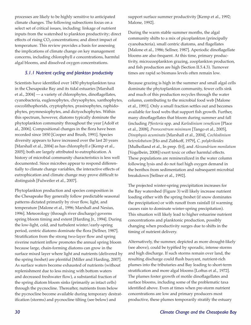
Climate Change and the Chesapeake Bay�0
processes are likely to be highly sensitive to anticipated climate changes. The following subsections focus on a select set of critical issues, including: linkage of nutrient inputs from the watershed to plankton productivity; direct effects of rising CO2 concentrations; and direct impact of temperature. This review provides a basis for assessing the implications of climate change on key management concerns, including chlorophyll a concentrations, harmful algal blooms, and dissolved oxygen concentrations.
5.�.� Nutrient cycling and plankton productivity
Scientists have identified over 1450 phytoplankton taxa in the Chesapeake Bay and its tidal estuaries [Marshall et al., 2004] — a variety of chlorophytes, dinoflagellates, cyanobacteria, euglenophytes, chrysophytes, xanthophytes, coccolithophorids, cryptophytes, prasinophytes, raphido-phytes, prymnesiophytes, and dictyochophytes. Within this spectrum, however, diatoms typically dominate the phytoplankton community throughout the year [Adolf et al., 2006]. Compositional changes in the flora have been recorded since 1850 [Cooper and Brush, 1991]. Species diversity appears to have increased over the last 20 years [Marshall et al., 2004] as has chlorophyll a [Kemp et al., 2005]; both are largely attributed to eutrophication. A history of microbial community characteristics is less well documented. Since microbes appear to respond differen-tially to climate change variables, the interactive effects of eutrophication and climate change may prove difficult to distinguish [Fulweiler et al., 2007].
Phytoplankton production and species composition in the Chesapeake Bay generally follow predictable seasonal patterns dictated primarily by river flow, light, and temperature [Malone et al., 1996; Marshall and Nesius, 1996]. Meteorology (through river discharge) governs spring bloom timing and extent [Harding Jr., 1994]. During the low-light, cold, and turbulent winter/early-spring period, centric diatoms dominate the flora [Sellner, 1987]. Stratification from the strong two-layer flow and spring riverine nutrient inflow promotes the annual spring bloom because large, chain-forming diatoms can grow in the surface mixed layer where light and nutrients (delivered by the spring freshet) are plentiful [Miller and Harding, 2007]. As surface waters become exhausted of nutrients (without replenishment due to less mixing with bottom waters and decreased freshwater flow), a substantial fraction of the spring diatom bloom sinks (primarily as intact cells) through the pycnocline. Thereafter, nutrients from below the pycnocline become available during temporary destrat-ification (storms) and pycnocline tilting (see below) and
support surface summer productivity [Kemp et al., 1992; Malone, 1992].
During the warm stable summer months, the algal community shifts to a mix of picoplankton (principally cyanobacteria), small centric diatoms, and flagellates [Malone et al., 1986; Sellner, 1987]. Aperiodic dinoflagellate blooms are also frequent. At this time, primary produc-tivity, microzooplankton grazing, zooplankton production, and fish production are high (Section II.5.4.3). Turnover times are rapid so biomass levels often remain low.
Because grazing is high in the summer and small algal cells dominate the phytoplankton community, fewer cells sink and much of this production recycles through the water column, contributing to the microbial food web [Malone et al., 1991]. Only a small fraction settles out and becomes available for food webs that support fish growth. Further, many dinoflagellates that bloom during summer and fall (including Pfiesteria spp. and Karlodinium veneficum [Place et al., 2008], Prorocentrumminimum [Tango et al., 2005], Dinophysisacuminata [Marshall et al., 2004], Cochlodiniumheterolobatum [Ho and Zubkoff, 1979], C.polykrikoides [Mulholland et al., In prep. (b)], and Alexandriummonilatum [Vogelbein, 2008]) exert toxic or other harmful effects. These populations are remineralized in the water column following lysis and do not fuel high oxygen demand in the benthos from sedimentation and subsequent microbial breakdown [Sellner et al., 1992].
The projected winter-spring precipitation increases for the Bay watershed (Figure 3) will likely increase nutrient loading either with the spring freshet (if snow dominates the precipitation) or with runoff from rainfall (if warming causes rain to dominate winter-spring precipitation). This situation will likely lead to higher estuarine nutrient concentrations and planktonic production, possibly changing when productivity surges due to shifts in the timing of nutrient delivery.
Alternatively, the summer, depicted as more drought-likely (see above), could be typified by sporadic, intense storms and high discharge. If such storms remain over land, the resulting discharge could flush buoyant, nutrient-rich plumes into the tributaries and Bay leading to short-term stratification and more algal blooms [Loftus et al., 1972]. The plumes foster growth of motile dinoflagellates and surface blooms, including some of the problematic taxa identified above. Even at times when pre-storm nutrient concentrations are low and primary producers most productive, these plumes temporarily stratify the estuary

Climate Change and the Chesapeake Bay ��
and pump nutrients into the system [see above; Malone et al., 1991].
In contrast to overland storm passage, intense storms passing over the Bay and tributaries would likely mix the water column and produce optimal conditions for diatom growth, not unlike the conditions and floral response that occur during fall overturn in the mesohaline Bay [Sellner, 1987]. Climate change, therefore, might shift the annual sequence to one with a larger-than-average spring diatom bloom, followed by small cells during the summer drought, interspersed with aperiodic dinoflagellate blooms or diatom maxima from storm passage.
Wind direction may also modify surface production during the summer when annual productivity reaches its maximum. Should these summer/fall storms be accom-panied by dramatic shifts in wind direction, from the normally dominant west direction to northerly or southerly along the Bay’s axis, frequent pycnocline tilting could occur. This tilting would pump sub-pycnocline nutrients into surface waters fostering shoreline blooms of diatoms and dinoflagellates [Malone et al., 1986; Sellner and Brownlee, 1990; Weiss et al., 1997]. The dinoflagellates don’t fall to the bottom; they decompose in the water, supporting microbial production. Further, wind speed and direction help determine upwelling and downwelling along the coast, so the timing of high-flow events relative to the dominant oceanic wind regime will influence the impact of the plume on the coastal ocean [Filippino et al., 2008].
5.�.� CO� effects on phytoplankton
CO2 can directly stimulate the growth of phytoplankton that do not have carbon-concentrating mechanisms (CCMs). CO2 is the preferred form of carbon for the principle carbon-fixing enzyme, ribulose-1,5-bisphosphate carboxylase-oxygenase (Rubisco). Most of the dissolved inorganic carbon in seawater, however, is bicarbonate ion (HCO3
-). Consequently, most cells have various CCMs to concentrate CO2 near active Rubisco sites. Species without CCMs are likely to benefit directly from CO2 increases (Figure 1).
Additionally, different forms of Rubisco have different affinities for CO2. Many of the bloom-forming microalgae are dinoflagellates, which appear to have a form of Rubisco with a low affinity for CO2 compared to the Rubisco in most other microalgae [Ratti et al., 2007; Whitney and Yellowlees, 1995]. CO2 increases might alleviate the carbon limitation of Rubisco and allow higher growth rates of
these dinoflagellates, increasing the number of harmful algal blooms throughout the system.
Evidence for CO2 limitation of productivity and growth occur during bloom conditions when rates of phytoplankton consumption of CO2 exceed atmospheric re-supply [Loftus et al., 1979]. Accompanied by a pH increase, this change could lead to species selection because some taxa are better able to cope with both elevated pH and low pCO2 (e.g., Prorocentrumminimum, Microcystisaeruginosa) [Hansen, 2002; Seitzinger, 1991]. However, scientists know little about the range of tolerances of most algal species or how they will respond as part of an ecosystem. Further, there is limited information about how other taxa might respond to changes in pCO2 (or temperature or the combined effects), and how these responses affect compet-itive interactions.
Riebesell et al. [1993] demonstrated that diatom growth can be limited by CO2, similar to reports of enhanced diatom growth under elevated CO2 [Tortell et al., 2002]. In other work, CO2 stimulated cyanobacterial growth and N2 fixation for various diazotrophic taxa [Fu et al., 2008a; Hutchins et al., 2007; Levitan et al., 2007]. Diazotrophic organisms have been shown to fix substantial new nitrogen in the Chesapeake Bay plume and surrounding coastal waters [Mulholland et al., 2007; Mulholland et al., In prep. (a)], suggesting that increasing CO2 could significantly affect biogeochemical cycles. In addition to diazotrophic cyanobacteria, Synechococcus growth as well as growth of the raphidophyte, Heterosigmaakashiwo, were stimulated under both high-CO2 and high-temperature scenarios [Fu et al., 2008a; Fu et al., 2008b]; P.minimum was less affected [Fu et al., 2008b].
Secondary effects of higher CO2 and enhanced phyto-plankton production might include enhanced carbohydrate production and release. Since CO2 enhances photosyn-thetic carbon fixation by some phytoplankton, increases in carbohydrate release may also occur. Such increases might stimulate bacterial production or promote aggregation and settling of material [Riebesell, 2004]. This situation, in turn, favors heterotrophic production through elevated water column and benthic metabolism (largely microbial), further expanding the current dissolved oxygen problems of the deeper Bay (Section II.5.1.5).
5.�.� Temperature effects on plankton
In addition to CO2 effects, temperature is important in regulating phytoplankton growth. In general, higher

Climate Change and the Chesapeake Bay��
growth rates occur at higher temperatures within a given species’ temperature range; however, more subtle impacts are likely as well. For example, temperature affects species succession, with small phytoplankton becoming dominant as temperatures rise [Sommer et al., 2007].
Asynchronous changes in the timing of seasonal events, such as spring phytoplankton blooms [e.g., Wiltshire and Manly, 2004] and the response of associated grazers, also occur. The result is a decoupling of the historic relation-ships between grazers and their food [Edwards and Richardson, 2004]. In particular, high-latitude systems now have earlier spring blooms. This shift in timing affects grazers’ ability to “keep up,” thereby altering the particle rain to the benthos [Edwards and Richardson, 2004]. Further, combined effects of eutrophication and climate change have contributed to a system-wide shift from net denitrification to net N2 fixation in the Narragansett estuary [Fulweiler et al., 2007], with important implications for the nutrient inventories in estuaries and coastal systems.
In the Chesapeake Bay, blooms of some potentially harmful taxa are occurring earlier and expanding their range [Marshall, 2008]. For example, an extensive Cochlodiniumpolykrikoides bloom occurred in August 2007 in the lower Chesapeake Bay system, which proved toxic to juvenile fish and oysters [Mulholland et al., In prep. (b)]. The recent whelk kill associated with the first recorded bloom of toxin-producing Alexandriummonilatum [Vogelbein, 2008] in the York River further exemplifies potential range expansion for problematic harmful algal species. Should blooms of these organisms continue to expand their range or impinge on larval recruitment seasons, impacts to higher trophic levels could be profound.
Temperature increases are likely to affect the metabolic status of the Chesapeake Bay. In a synthesis of microbial rate measurements in the Chesapeake Bay, Lomas et al. [2002] found that planktonic respiration increases more rapidly than does photosynthesis with temperature. Their results suggest that the Bay might become net hetero-trophic on an annual time scale, reversing its current net autotrophic status [Smith and Kemp, 1995]. This potential shift is consistent with the concepts described above in which increased heterotrophy might result from bacterial decomposition of carbohydrates. Carbohydrate production would be enhanced due to higher levels of phytoplankton photosynthesis in response to elevated CO2 as well as lysis of dinoflagellates in the water rather than the benthos [Sellner et al., 1992].
5.�.� Harmful algal blooms and pathogens
The Chesapeake Bay and its tributaries, with their spring-fall stratification and nutrient-rich conditions, constitute ideal environments for bloom-forming dinoflagellates [see Margalef, 1978; Sellner et al., 2001]. Further, for marine, bloom-forming phytoplankton, “warmer water tempera-tures can encourage a shift in species composition of algae toward the more toxic dinoflagellates” (quote from Haines et al. [2000] and attributed to Valiela [1984]). Toxic bloom increases in Asia associated with the warm phase of El Niño also support this contention [Hallegraeff, 1993]. Further, paleontological evidence associates dinoflagellate dominance with warmer ocean surface waters [Dale, 2001; Mudie et al., 2002].
Stratification may also play a role in algal community structure. Peperzak [2003] conducted several experiments with brackish bloom-forming and non-bloom-forming taxa under simulated stratified conditions and a 4° C temperature increase. In these experiments, a cosmopolitan contributor to estuarine systems (Skeletonemacostatum) was not perturbed by the shift to stratified conditions, suggesting that this common winter-spring taxon in the Bay would remain a key contributor to spring production. However, P.minimum, the spring co-dominant in the Chesapeake and occasional toxin producer [see Luckenbach et al., 1993], and two raphidophytes (Heterosigma spp.) found in mid-Atlantic coastal bays were stimulated by the increased stratification and temperature. This response suggests that more frequent blooms will occur under these climate change conditions [Fu et al., 2008b]. North Sea data echo this potential preference for bloom associated with expected climate-induced changes in stratification and temperature. These data indicate that dinoflagellate maxima have occurred earlier in recent years, compared to those in the late 1950s — attributable to the increasing strat-ification and temperature [Edwards and Richardson, 2004]. Similarly, Johns et al. [2003] suggested that increasing contributions of dinoflagellates near Georges Bank in the Gulf of Maine likely resulted from increasing stratification and stability in the area due to progressive freshening.
Shifts in algal taxonomic composition from flow-induced stratification pose potential problems, both in terms of altered food web structure and toxicity to trophic groups. Projected changes could increase production by dinofla-gellates (noted above) — a group associated with altered tropho-dynamics — through several mechanisms. Some taxa can reduce zooplankton grazing and fecundity through poor food quality [e.g., Harvey et al., 1989] or
Climate Change and the Chesapeake Bay ��
production of toxins or grazing-deterrent compounds [e.g., Adolf et al., 2007]. Very high cell abundances can also reduce grazing pressure from co-occurring zooplankton populations [e.g., Sellner and Olson, 1985]. Pelagic bacterial production may increase due to lysis of dinoflagellates largely in the water rather than the benthos [Sellner et al., 1992]), favoring heterotrophic flagellates over copepods. Consequently, the microbial food web gains importance, diminishing the classical food chain that supports fish production.
Additional impacts of an altered climate — specifically prolonged droughts [Hayhoe et al., 2007] — will also likely increase introduction of coastal phytoplankton, including several harmful taxa. Droughts will lead to lower freshwater flows with greater oceanic intrusion into the Bay, elevating salinity levels further north in the system and bringing unique taxa to the region. This situation developed in the spring and summer of 2002 following the drought from 1999 to 2002. With oceanic intrusion into the mid-Bay, coastal populations of Dinophysisacuminata moved into the lower Potomac River estuary [Marshall et al., 2004], causing fear of okadaic acid intoxication and diarrhetic shellfish poisoning for the oyster-consuming public. Climate-induced drought might, therefore, prompt more frequent toxic algal blooms, which are currently rare in the system.
The leafy chlorophyte Enteromorpha, a macroalga, is stimulated by elevated water temperatures [Lotze and Worm, 2002]. A similar taxon, Ulva, is characteristic of eutrophic estuaries including the Chesapeake and its tributaries. Conceivably, warmer winters and springs might favor earlier growth of these two macroalgae, which could foul shorelines and submerged vegetation, clog commercial fish nets, and cause hypoxic conditions in sheltered bays following storms and high winds. Further, Kana et al. [2004] associated decay of these blooms with the onset of other harmful algal blooms, such as Aureococcusanophagefferens.
Bacteria also respond to temperature changes. Some true heterotrophic bacteria, such as the Vibriospecies, are associated with serious illnesses, including gangrene and sepsis. Pathogenic species, such as Vibrio vulnificus and V.cholerae, have been identified in Chesapeake Bay waters (summarized in Rose et al. [2000]). Colwell [1996] and McLaughlin et al. [2005] suggested an association of V.cholerae and V.parahaemolyticus with elevated sea surface temperatures. Further, Mouriño-Pérez et al. [2003] showed that growth of a free-living strain of this bacterium
was stimulated by a coastal dinoflagellate bloom off of California, reaching levels three orders of magnitude higher than the known minimum infectious dose. This scenario indicates that climate-change-induced increases in harmful algal blooms (see above) might threaten human health, either directly or through the fueling of pathogen growth from bloom organic matter. Taxon-specific relation-ships between phytoplankton and bacteria require further investigation.
Shellfish ingestion and concentration of pathogenic bacteria can also lead to outbreaks of gastroenteritis and death (with V. vulnificus) in some human consumers (see references in Rose et al. [2000]). Increasing temperatures in the Bay would favor these bacteria (references above), increasing the threat of this disease in the basin. Reports from the Centers for Disease Control and Prevention (CDC) summarized from state monitoring indicate a recent local trend consistent with the high-temperature selection for the genus1. In the summer of 2005, water temperatures were 2 to 3° C higher than the summers of 2003 and 2004. Vibrio outbreaks totaled 26 in Maryland for the warmer summer versus zero and two outbreaks, respectively, for 2003 and 2004. Although the data set is small, the increasing number of incidences of this taxon with higher water temperatures locally is consistent with the prevalence of the bacterium in warmer waters noted above and may foreshadow future conditions as climate-change-induced temperatures rise.
5.�.5 Dissolved oxygen
Dissolved oxygen levels constitute a key measure of the Chesapeake’s health. Although seasonal hypoxia is a natural feature of the estuary, the size, frequency, and severity of hypoxic conditions signify the degree of human impact on the ecosystem.
Hypoxia results from the interplay between two factors: sinking of the spring phytoplankton bloom, which fuels bottom respiration; and density stratification, which inhibits the mixing that replenishes deeper waters with oxygen [Hagy et al., 2004; Malone et al., 1996]. In summer, plankton deposition (as zooplankton fecal pellets, larger diatoms, and other algal debris) continues at rates suffi-cient to maintain respiration and low O2 (< 2 mg l-1) [e.g., Kemp et al., 1999; Newell et al., 2007]. The significant trend of increasing intensity, duration, and extent of hypoxic conditions since 1950 relates to increased nutrient loading from human activities in the watershed [Boesch et al., 2001; Hagy et al., 2004; Kemp et al., 2005; Malone, 1992].1 www.cdc.gov

Climate Change and the Chesapeake Bay��
Climate change may also contribute to changes in the spatial and temporal distribution of hypoxic conditions. Hagy et al. [2004] found the Susquehanna River’s January-to-May average flow a good predictor of the subsequent summertime volumes of low-oxygen water. Hagy et al.’s functional fits to the data suggest that a 10% increase in flow will increase the volume of anoxic water (< 0.2 mg l-1) by 10%, severely hypoxic water (< 1.0 mg l-1) by 6%, and mildly hypoxic water (< 2.0 mg l-1) by 3%. Najjar [2008] showed that the January-to-May flow of the Susquehanna River strongly correlates with January-to-May watershed precipitation, and that fractional flow and precipitation changes are equal. Thus, the likely increases in winter-spring precipitation projected over the 21st century (Figure 3) could result in summertime oxygen declines. If nutrient loading increases with precipitation in the non-linear manner that Howarth et al. [2006] suggested (Section II.3.2), then plankton production and hypoxia will increase further.
Lower O2 solubility in the warmer summer waters would contribute to further reductions in bottom-water O2 concen-trations [e.g., Sampou and Kemp, 1994]. The sensitivity of the oxygen saturation concentration to temperature (d[O2]sat / dT) increases as water cools (i.e., oxygen declines for a given temperature increase are greater at lower temperatures). The climatological temperature range in the mainstem Chesapeake Bay is approximately 2 – 27° C, with a corresponding range in d[O2]sat / dTof -0.34 to -0.13 mg l-1 ° C-1 (S = 15 ppt). Thus, for a projected warming of 2 – 5° C by 2100 (Figure 4b), the estimated decrease in O2 concen-tration is 0.7 – 1.7 mg l-1 during the coldest months and 0.3 – 0.7 mg l-1 during the warmest months. The difference in oxygen concentration between severely hypoxic and anoxic waters is 0.8 mg l-1. At the temperature of sub-pycnocline waters in July (~20° C), d[O2]sat / dT is equal to -0.16 mg l-1 °C-1. A warming of about 5° C, therefore, will make waters that are currently hypoxic turn anoxic solely due to solubility.
Higher temperatures would also tend to accelerate rates of nutrient recycling, further stimulating phytoplankton production and potential deposition [e.g., Kemp et al., 2005]. Coupled with the suggested shift towards greater heterotrophy with warming [Lomas et al., 2002], this accel-erated recycling would drive oxygen concentrations even lower. Simulation modeling studies for the northern Gulf of Mexico support these hypothesized responses of bottom water hypoxia to climate change scenarios [Justić et al., 1996; 2003].
5.2 Submerged aquatic vegetation
Communities of seagrasses and related submerged aquatic vegetation (SAV) in the Chesapeake Bay are highly sensitive to changes in environmental conditions, including salinity and temperature. Historically, more than 15 species of SAV inhabited the Bay. One of these plants, eelgrass (Zosteramarina), is a globally dominant north-temperate seagrass. Although eelgrass has a moderate salinity tolerance range (~15 – 40 ppt), the species is confined to the higher salinity regions of the lower Bay. The only other true seagrass in the Bay is widgeon grass (Ruppiamaritima), a highly adaptable euryhaline (salinity tolerance of 0 – 45 ppt) pioneer plant that inhabits coastal waters from Maine to Texas [Kantrud, 1991]. All other SAV species in the Bay are freshwater plants (they evolved in purely freshwater habitats) [Stevenson and Confer, 1978], with modest salt tolerance (in general, S < 15 ppt).
At least half of these species, including the two seagrasses, remain in the Bay today, although at levels greatly reduced from the past [Moore et al., 2000]. Most of the Bay’s SAV populations have similar annual cycles of abundance, with summer peaks and growing seasons extending from spring through fall. The Bay’s eelgrass population differs because it is near the southern limit of its geographic distribution. Consequently, eelgrass exhibits a bimodal seasonality in biomass and growth, with late-spring and mid-fall peaks and summer minima that reflect limited tolerance for high temperatures [Wetzel and Penhale, 1983].
Light availability is a primary factor regulating SAV abundance and spatial distribution, particularly in inherently turbid estuarine systems such as the Chesapeake Bay [Kemp et al., 2005]. Minimum light requirements for survival of SAV are ten to 20 times higher than those of algae [e.g., Dennison et al., 1993]. A major decline in the Chesapeake Bay’s SAV abundance, beginning in the mid-1960s [Orth and Moore, 1983], appears to be largely attributable to widespread decreases in water clarity and increases in nutrient concentrations throughout the estuary [e.g., Kemp et al., 1983; Moore and Wetzel, 2000; Twilley et al., 1985]. Higher turbidity associated with increased runoff of nutrients and sediments inhibits seagrass growth due to reduced light availability [e.g., Kemp et al., 2005; Quammen and Onuf, 1993; Twilley et al., 1985]. This sensitivity may be particularly problematic in the context of climate change given the possibility of significant increases in sediment loading from greater and more episodic precipitation, as discussed previously in Sections II.2.3 and II.3.1.

Climate Change and the Chesapeake Bay �5
SAV species exhibit widely varying sensitivity to temperature change, with optimal growth temperatures ranging from 22 – 25° C for eelgrass [e.g., Bintz et al., 2003] to 30 – 35° C for various freshwater plants in brackish habitats [Santamaría and van Vierssen, 1997]. Increasing temperatures in New England coastal waters seem to have rendered eelgrass stands more susceptible to light stress associated with nutrient enrichment and overgrowth by epiphytic algae [Bintz et al., 2003]. An extended hot period with daily peak water temperatures exceeding 33 – 35° C [Orth and Moore, 2008] appears to have triggered a massive eelgrass die-off in the Bay during the summer of 2005. High temperatures and limited water column mixing may have contributed to internal oxygen deficiency in eelgrass plants, degradation of meristematic tissue, and mortality [Greve et al., 2003].
In broad terms, interannual variations in SAV distribution and abundance correspond to fluctuations in freshwater flow. For example, in the Choptank River estuary, low flow tends to be associated with higher plant abundance [Stevenson et al., 1993]. Similarly, an inferred long-term (multi-decade) data record on seagrass growth and rainfall in the Mediterranean littoral zone reveals a strong inverse correlation, suggesting that fresh water negatively affects seagrass [Marba and Duarte, 1997]. For some seagrasses, reduced salinity due to high freshwater input to coastal waters tends to cause osmotic stress for these halophytes [e.g., Fourqurean et al., 2003]. Conversely, reductions in salinity may stimulate the growth of other brackish-water SAV [e.g., Stevenson et al., 1993].
The resurgence of widgeon grass in the Choptank River in 1985 after a four-year drought and a second explosive spread from 1993 to 1997 following a shorter (two-year) drought provides another example of SAV sensitivity to flow [Kemp et al., 2005]. One theory is that the period of relatively clear waters and low nutrients associated with the low flows from 1980 to 1983 proved sufficient for small beds in tertiary tributaries to flourish. These beds may have served as key seed sources for transport to the open Choptank, where clear waters allowed rapid growth and dispersal of these pioneer plants and formation of large contiguous beds.
By the time the second brief drought period occurred, the well-established beds could exploit fully the improved water quality, creating a second burst that peaked in 1997. Since this time, widgeon grass beds in the mesohaline Choptank appear sufficiently established to maintain seed banks that allow this light-sensitive species to expand
and contract with the clear and turbid waters associated, respectively, with low- and high-flow years. This finding may explain why correlations between Secchi depth and SAV cover are highly significant after 1996 but non-existent before this time.
In addition to temperature, salinity, and light, SAV is sensitive to CO2 concentration. Palacios and Zimmerman [2007] showed that eelgrass biomass increased in response to elevated CO2 levels under light-replete conditions during a year-long incubation. For an approximate doubling of CO2 concentration above current levels, shoot biomass increased by 25%. No response occurred under light-limiting conditions, however, which suggests that CO2 increases could aid restoration only if measures to maintain sufficient water clarity take place concurrently.
5.3 Estuarine wetlands
The Chesapeake Bay’s shoreline represents one of its most threatened resources — one that is subject to the combined impacts of climate and land use change [Maryland Department of Natural Resources, 2000]. Coastal marshes and shoreline ecosystems provide important ecological functions, serving as nursery areas, sources of dissolved organic carbon, critical habitat, modifiers of local water quality, and stabilizers of global levels of available nitrogen, atmospheric sulfur, carbon dioxide, and methane [Mitsch and Gosselink, 2000]. Rising sea levels, changes in storm regimes, altered salinity regimes, CO2 fertilization and other climate-related factors, as well as continued land use change and shoreline hardening, will further stress already threatened coastal wetlands [Rogers and McCarty, 2000; U.S. EPA, 2002]. These ecosystems exist in a naturally dynamic environment; however, the current (and forecast) rate of change is likely to overwhelm their inherent resilience [Fisher et al., 2000].
Inundation by rising sea level poses one of the most direct threats for regional coastal and estuarine wetlands. The amount of land inundated by a given rise in sea level is a complex function of elevation, shoreline geology, land use, wetland ecology, and the rate of sea-level rise. Current inundation estimates of the lands bordering the Bay rely on elevation changes that correspond to projected sea-level-rise estimates of 0.7 – 1.6 m (Section II.2.5). Using digital elevation models (DEMs) and shoreline data, Titus and Richman [2001] estimated that about 2500 km2 of land lies below the 1.5-m elevation contour in Virginia and Maryland (essentially the shores of the Bay). Wu et al. [2008] used DEMs with finer (30-m) horizontal resolution

Climate Change and the Chesapeake Bay��
to estimate that 1700 km2 of land in Virginia and Maryland lies below the 0.7-m contour; about half of this area is wetlands.
The current forecasts for the rates of sea-level rise in the Chesapeake Bay are significantly greater than rates over the last several centuries (Section II.2.5). How much of the existing wetland in the Bay region will be able to either accrete vertically or migrate horizontally sufficiently fast to keep pace with the accelerated rate of change remains unclear [Kearney et al., 1988; Kearney et al., 1994; Reed et al., 2008; Stevenson et al., 1985]. Extensive wetlands along the Bay’s main stem, such as the Blackwater Wildlife Refuge in Maryland and the Guinea Marshes in Virginia, already have less vegetative cover due to inundation and erosion. Changes in the vegetative community composition of the extensive oxbow wetlands at the headwaters of the Bay’s tidal tributaries seem related to increased inundation frequency, a sign that the wetlands are not keeping pace with rising sea level [Perry and Hershner, 1999].
Wetlands also respond to elevated levels of atmospheric CO2, increasing temperatures, and changing salinity patterns. A Scirpusolneyi wetland sedge community of the Rhode River, exposed to an approximate doubling of atmospheric CO2 over 17 years, had enhanced shoot density, shoot biomass, and rates of net CO2 uptake (also known as net ecosystem exchange) compared to ambient exposures [Rasse et al., 2005]. In contrast, Spartinapatens shows no significant response to CO2 [Erickson et al., 2007]. Rasse et al. [2005] also clearly documented salinity stress on S.olneyi, with significant anti-correlations at the inter-annual time scale between salinity and the three growth measures referred to above. Elevated CO2 stimulation of plant growth has important implications for brackish marshes, many of which are dominated by C3 plant species such as Scirpusolneyi. Indeed, recent results from a Rhode River marsh [Megonigal, 2008] showed that higher CO2 levels increase root biomass, which raises the elevation of the tidal marsh soil. The increase in elevation was ~3 mm yr-1, which is comparable to current rates of relative sea-level rise in the Chesapeake Bay. Thus, elevated CO2 may stimulate marsh accretion and ameliorate marsh losses projected from accelerated sea-level rise. The joint effect of temperature increases and elevated CO2 concentrations may produce different changes to marshes than elevated CO2 alone, but we know little about these interactions.
Ongoing land use change and associated shoreline hardening compound the impact of rising sea level. Recent shoreline situation reports show a high percentage
of hardened shoreline across the Bay region.2 Shoreline hardening restricts marshes from migrating shoreward in response to sea-level rise. Detailed studies linking sea-level rise, land use change, and shoreline condition are very limited for the Chesapeake Bay. Dingerson [2005] used a combination of regression and fuzzy-logic-based methods to provide shoreline development scenarios for a section of southern Virginia through 2025. This approach parallels techniques used for Baywide land use and land cover scenarios. The study illustrates the potential for evaluating the consequences of development for shoreline condition; however the approach has not yet been used on larger areas and which regions may prove most vulnerable remains unclear.
Inundation of coastal wetlands by rising sea levels may stress the systems in ways that enhance invasion of less desirable species such as Phragmitesaustralis (one of six species identified as causing, or having the potential to cause, significant degradation of the aquatic ecosystem of the Bay) [U.S. Environmental Protection Agency, 2008c]. Reported impacts include significant loss of plant diversity [Chambers et al., 1999; Meyerson et al., 2002; Warren et al., 2001], changes in marsh hydrology with the development of Phragmites stands [see Marks et al., 1994], and a reduction in insect, avian, and other animal assemblages [Chambers et al., 1999; Osgood et al., 2002]. Shifts within native plant communities are also probable, although they are difficult to predict with current experi-mental data [Dukes, 2007]. Species may show increased resilience to change under elevated CO2 when exposed to adverse environmental conditions, as discussed above. Additionally, for many marsh systems to persist, suspended sediment from inflowing streams and rivers is necessary for soil accretion. Climate change might result in changed timing and overall delivery of sediment from upstream sources, but these consequences remain uncertain.
5.4 Fish and shellfish
Historic and contemporary climate variability provides valuable information for understanding how climate change influences fish and shellfish species, along with other aspects of the Bay, through alteration of well-known variables and processes. This section focuses on temper-ature, salinity, plankton production, dissolved oxygen, and sea level since climate change is likely to affect these variables, transforming the Bay ecosystem by altering the
2 InformationforMarylandandVirginiacoastlinesisavailableat:ccrm.vims.edu

Climate Change and the Chesapeake Bay ��
health, distribution, and abundance of ecologically and economically important fish and shellfish species.
5.�.� Temperature impacts on fish and shellfish
The Chesapeake Bay lies near the boundary of warm-temperate and cold-temperate climate provinces and is influenced by both continental and oceanic air masses. Warming will differentially affect warm- and cold-temperate species that use the Bay as a seasonal feeding ground or nursery area. Species with more southerly distri-butions and temperature tolerances will likely benefit from higher temperatures and some may intensify their use of the Bay as feeding and spawning grounds and as a nursery area [Austin, 2002; Wood, 2000]. Conversely, warming will limit the Bay’s use by some cold-temperate species. This latter situation is consistent with recent patterns of menhaden recruitment in Atlantic coast estuaries, which suggest the possibility of a northward shift in the major locations of Atlantic menhaden spawning [Houde, 2008]. Higher temperatures can decrease the areal extent of bioenergetically favorable Bay habitats for cold-temperate species during the growing season due to the direct effects of increased temperatures and because higher temperatures decrease dissolved oxygen content (Section II.5.1.5) and increase metabolic costs (Section II.5.4.4). Developing fish embryos cannot temperature-compensate and tend to have narrower temperature tolerances than other life stages. As a result, the thermal tolerances of embryos may become particularly important in determining shifts in species distributions [Rombough, 1997].
Northward range expansions by warm-water species may either enhance or impair fisheries. Shrimps of the genus Farfantepenaeus, which now support important fisheries in North Carolina [Hettler, 1992], could increase and support viable fisheries in the Chesapeake Bay and elsewhere in the Mid-Atlantic Bight. Increasing temperatures, along with other climate-related changes in the Bay environment, however, may simultaneously facilitate successful northward expansion of non-native species [Stachowicz et al., 2002] and pathogens [Cook et al., 1998].
In addition, physical or ecological factors other than temperature may preclude a smooth transition to a balanced ecosystem dominated by warm-water fishery species. For example, many Bay species depend on coastal and estuarine circulation patterns to distribute their planktonic egg and larval stages into suitable nursery areas [e.g., Epifanio and Garvine, 2001]. Predicting future changes in coastal or Bay circulation patterns remains
difficult because freshwater inflow, sea level, surface wind fields, and coastal landforms will also influence the evolution of these patterns (Section II.4.1). Altered currents may prove especially important in affecting the rate of spread by less mobile or coastal-spawning warm-water shellfish and fish species into the Bay. In addition, oligo-haline/upper-mesohaline species (such as the bivalves Mytilopsisleucophaeata or Ischadiumrecurvum) that live only in estuaries may spread northward slowly if they cannot tolerate the marine conditions that occur between estuaries.
Species at their southernmost range in the Mid-Atlantic region will be eliminated from the Chesapeake Bay if water temperatures reach levels that are either lethal or inhibit successful reproduction. For example, the commercially important soft clam, Myaarenaria, in the Chesapeake Bay is near its southern distribution limit and may be extir-pated if temperatures approach and remain near ~32° C [Kennedy and Mihursky, 1971]. Non-fisheries species with significant impact on the Chesapeake Bay food web may also be negatively affected by increasing temperatures. Lethal temperature for the lobate ctenophore, Mnemiopsisleidyi, collected from the Chesapeake Bay is approximately 30° C in laboratory experiments [Breitburg, 2002]. This ctenophore extends through the tropics to South America, however, suggesting selective use of more oceanic waters and adaptation as possible responses to warming.
A persistent long-term rise in water temperatures is also likely to alter the seasonal distribution patterns of ecologically and economically important fish and shellfish species of the Chesapeake Bay. Warming will likely result in a shorter winter season and may allow earlier spring immigration and later fall emigration of some coastal species (e.g., see Frank et al. [1990] for the St. Lawrence region). Spawning migrations of American shad (Alosasapidissima) may be particularly sensitive to changes in seasonal patterns of water temperatures. American shad now migrate up the Columbia River (where they were introduced) 38 days earlier than during the 1950s as water temperatures have increased due to reductions in spring flow by the Bonneville Dam [Quinn and Adams, 1996].
Higher water temperatures in winter may have positive effects on some species. The overwintering mortality of juvenile fishes can be an important contributing factor to year-class strength [Conover and Present, 1990]. For example, interannual variation in Atlantic croaker (Micro-pogoniasundulatus)catches has been linked to winter temperatures with higher temperatures resulting in greater juvenile overwintering survival and stronger year classes

Climate Change and the Chesapeake Bay��
[Hare and Able, 2007]. Severe winters may have resulted in low catches of blue crab [e.g., Pearson, 1948] and recent studies highlighted the importance of overwintering mortality to both juveniles [Bauer, 2006] and adults [Rome et al., 2005] of this species in the Bay.
As with direct effects, indirect food web effects of increasing temperatures could either benefit or have deleterious effects on native fish and shellfish. Alteration in winter-summer warming relative to seasonal day lengths could affect fisheries by changing the timing of the spring bloom relative to the reproduction period of late-winter- and spring-spawning fishes. Such shifts could create a mismatch (described by Cushing [1975; 1990]) between the nutritional requirements of larval fishes and the abundance peak of their zooplankton prey. For some species, warming trends could possibly improve the match between prey availability and fish reproduction. In either case, climate-induced changes in the frequency of matched prey abundance and larval-feeding demand, as well as the ability of local populations to adapt to local prey condi-tions, are likely important since early life history stage mortality rates establish the annual recruitment in many fish populations [Houde, 1987].
Warming may also alter the activity and abundance of predators that feed on fish eggs and larvae. Strong evidence suggests that an increase in winter water temperatures may account for the winter flounder (Pseudopleuronectesamericanus) population decline in Narragansett Bay, Rhode Island. Keller et al. [1999] and Keller and Klein-MacPhee [2000] have shown that winter flounder egg and larval mortality rates are higher in warmer water than in cooler (3° C difference). In their mesocosm experiments, these authors note that egg and larval predators were more active and more abundant in warm water and that hatching winter flounder larvae were larger under colder condi-tions. Field sampling suggests that one important effect of increasing temperatures in Narragansett Bay was the increase in the temporal overlap between the ctenophore M.leidyi and early life stages of summer-breeding fishes, such as flounder, that serve as its prey [Sullivan et al., 2001]. In the Chesapeake Bay, M.leidyipeaks already coincide with reproduction by summer-breeding fishes and shellfish. Nevertheless, the underlying mechanisms illustrated by the Narragansett Bay example could prove important within the Chesapeake Bay food web as well.
Traditionally, the eastern oyster (Crassostreavirginica) has represented an important fishery species for the Bay. As recently as 1987, the Chesapeake Bay produced the
most oysters on the Atlantic and Gulf of Mexico coasts [Haven, 1987]. While overfishing has historically played a significant role in the demise of this fishery, two oyster pathogens — Perkinsusmarinus(Dermo) and Haplospo-ridiumnelsoni(MSX) — have contributed to the long-term decline. These pathogens have also hindered the popula-tion’s recovery despite considerable restoration effort [Andrews, 1996]. Increasing winter temperatures have already exacerbated these diseases in the oyster popula-tions of Atlantic Coast estuaries [Burreson and Ragone Calvo, 1996; Cook et al., 1998; Ford, 1996; Ford et al., 1999; Paraso et al., 1999]. The strong temperature dependence of Dermo, in particular, suggests that the Chesapeake region could experience increased parasite stress in subtidal oysters as water temperatures increase, but may simultane-ously experience an extension in the northerly extent of intertidal oysters [Malek, 2008]. Intertidal exposure during summer raises tissue temperatures to levels that are detri-mental to P.marinus, but within the physiological range of C.virginica[Malek, 2008; Milardo, 2001].
Some fish parasites might also benefit from warmer climes, likely through production of one or more additional gener-ations each year [Magnuson et al., 1997; Marcogliese, 2001]. Higher temperatures lead to deterioration of host body condition (e.g., lymphocytes decline, disease resistance decreases, and survivorship declines) [references in Marco-gliese, 2001]. Additionally, increasing temperature leads to faster development of planktonic and benthic invertebrates, enhancing parasite transmission [Chubb, 1982] as well as parasite diversity [Dobson and Carper, 1992]. Eutrophic conditions may alter this progression; lake work suggests increasing parasitism as eutrophication occurs followed by a decline with extreme eutrophication [Marcogliese, 2001]. Weisburg et al. [1986] documented increases in the intermediate host Limnodrilus sp. for the fish redworm Eustrongylides sp. (pathogenic to avian definitive hosts) in warming eutrophic waters of the Chesapeake. Fish infected included yellow perch (Perca flavescens) [Muzzall, 1999], which is common to the Bay. Warmer shelf waters might also lead to earlier arrivals and later departures of pelagic fishes [e.g., Frank et al., 1990], favoring transmission of pelagic parasites (as suggested for the St. Lawrence and Japan) and increasing human illness from pathogens trans-ferred via undercooked fish [Hubert et al., 1989].
Recent observations in upper river basins also indicate winter survival of potential pathogens. The upper Shenandoah River has had winter water temperatures substantially higher over the last four years. Each spring during this period, major smallmouth bass mortalities

Climate Change and the Chesapeake Bay ��
occurred. Winter pathogen survival is one possible explanation for these recurring events [Chesapeake Bay Foundation, 2007]. If this hypothesis is correct, overwintering success and subsequent spring illnesses or mortalities in some fish species may become increasingly common as regional water temperatures rise.
Warming might also influence pollutant impacts. For example, higher temperature-induced mercury methylation [Booth and Zeller, 2005] has been suggested as a possible mechanism increasing mercury uptake in fish [Bambrick and Kjellstrom, 2004; from McMichael et al., 2006]. Fsh tissue mercury concentrations already pose a public health concern in Chesapeake jurisdictions, especially given the potential fetal impacts of this toxic substance.
5.�.� Salinity impacts on fish and shellfish
Changes in sea level, temperature, and precipitation are likely to create significant changes in estuarine salinity patterns (Section II.4.2). The predominant direction of salinity change remains unclear, however, due to a lack of consensus on annual streamflow projections (Table 1). The most pronounced effects of altered salinity on fishery species will likely result from changes in the distribution and abundance of predators, prey, and pathogens.
Salinity affects the eastern oyster in several ways. First, the oyster has a physiological tolerance for salinities between 5 and 35 ppt. Second, mortality from Perkinsus and Haplo-sporidium infections is limited to salinities above about 12 ppt [Haven, 1987]. Model and field surveys indicate that flow-related salinity fluctuations between 10 and 20 ppt influence the range and infection rate of oysters by both pathogens [Burreson and Ragone Calvo, 1996; Cook et al., 1998; Ford, 1996; Paraso et al., 1999]. Third, spatfall success (recruitment) in the Bay oyster population is positively affected by higher salinity [e.g., Kimmel and Newell, 2007]. The net effect of these three factors in the face of salinity increases (which will very likely occur if precipitation remains unchanged) may depend on whether the combi-nation of favorable conditions for recruitment and high parasite stress affects selection for disease tolerance in infected oysters.
Another example of complex species interactions poten-tially affected by climate change that could influence the state of Chesapeake Bay fisheries involves the two dominant gelatinous zooplankton species within the Bay: the ctenophore M.leidyi and the scyphomedusa Chrysaoraquinquecirrha(the sea nettle) [Purcell and Arai, 2000]. Both
species feed directly on fish eggs and larvae [Cowan, Jr. and Houde, 1993; Govoni and Olney, 1991; Monteleone and Duguay, 2003] as well as on zooplankton that are important prey for adult forage fish and other fish species in early life stages [Burrell and Van Engel, 1976; Cargo and Schultz, 1966; Feigenbaum and Kelly, 1984; Purcell, 1992]. M.leidyihas a greater ability to deplete its prey than does C.quinquecirrha; it also feeds on oyster larvae. Inter-annual variability in salinity and flow strongly affect the timing of peak sea nettle abundance, with levels peaking earlier in years of above-average salinity [Breitburg and Fulford, 2006]. Consequently, climate change may ultimately influence the timing and magnitude of sea nettle consumption of icthyoplankton and other zooplankton, as well as indirect effects mediated through the control that sea nettles exert over their ctenophore, M.leidyi,prey.
5.�.� Plankton production impacts on fish and shellfish
Fisheries production in the Bay, as in most mid-latitude temperate systems, is linked to the annual cycle of primary production initiated by high early spring streamflow (Section II.5.1.1) [e.g., Cushing, 1975; 1990; Pope et al., 1994; Silvert, 1993]. The timing and magnitude of the spring zooplankton bloom is influenced by winter weather and spring streamflow [Kimmel et al., 2006; Wood, 2000]. This bloom provides food for young-of-the-year of spring spawning fishes and forage fish species that actively feed in the Bay in early spring. These small forage fishes constitute important prey for larger fishes and are directly influenced by salinity, dissolved oxygen, and zooplankton distribu-tions [Brandt et al., 1992; Jung and Houde, 2003].
A change in the timing of the spring freshet could alter fishery production. If, for example, the spring freshet should wane or occur during higher temperatures after the seasonal transition from a diatom-dominated to a flagellate-and-picoplankton-dominated assemblage, fishery production would likely be negatively affected [Wood, 2000]. An example of this occurred in 1989. Because the succession to a summertime phytoplankton community had already taken place when the freshet occurred, nutrients delivered by the delayed freshwater pulse promoted unusually strong production of picoplankton rather than a spring diatom bloom [Malone et al., 1991]. Since many economically important Bay species (e.g., summer flounder, striped bass, Atlantic menhaden) depend on spring zooplankton (which are supported by the spring diatom bloom) during their early life history stages, a delay in the timing of the spring freshet would likely negatively affect fisheries production in the estuary. Fisheries outside

Climate Change and the Chesapeake Bay�0
the Bay would also be affected because many of these species spend much of their lives in the coastal ocean. Though substantial uncertainty exists in future projec-tions of spring bloom timing, indications suggest that the spring freshet will occur earlier and be stronger in the future (Section II.2.4). The implications of such a change for Chesapeake Bay fisheries remain unclear.
5.�.� Dissolved oxygen impacts on fish and shellfish
Low dissolved oxygen affects the growth, mortality, distribution, and food web interactions of a wide range of organisms in the Chesapeake [e.g., Breitburg, 2002; Breitburg et al., 2003; Kemp et al., 2005]. Seasonal hypoxia causes mortality of benthic animals in the deeper parts of the Bay meaning that deep benthic macrofauna are essentially absent in the summer and depauperate during other times of the year [Holland et al., 1987; Sagasti et al., 2001]. Mortality of animals can also occur in shallow waters during episodic advection of hypoxic or anoxic bottom water shoreward [Breitburg, 1990] and where warm, calm conditions result in diel hypoxic events in shallow waters [Tyler and Targett, 2007].
In addition to increasing mortality directly, hypoxia may affect the ecosystem and its fisheries through the behavioral and physiological responses of organisms, altering trophic interactions over broad time and space scales [Breitburg et al., 2001]. Increases in summer temperatures and increased anoxia or hypoxia, for example, may exclude species such as striped bass and Atlantic sturgeon (Acipenseroxyrhynchus) from benthic feeding grounds and bioener-getically favorable cool, deep-water environments [Brandt and Kirsch, 1993; Coutant, 1985; Coutant and Benson, 1990; Niklitschek and Secor, 2005; Price et al., 1985; Secor and Gunderson, 1998]. Low dissolved oxygen can also alter trophic interactions that support fishery species by inhib-iting production of ecologically important zooplankton grazers [Roman et al., 1993], increasing some species’ susceptibility to predation [Breitburg et al., 1994; Breitburg et al., 1997] and providing predatory refuge to others [Sagasti et al., 2001]. Repeated exposure of deeper subtidal oyster populations off Calvert Cliffs, Maryland to low-oxygen bottom water depressed growth rates compared to the rates for oysters in shallower areas where exposure to low-oxygen water occurred less frequently [Osman and Abbe, 1994].
Warming may increase the extent and severity of hypoxia on macrofauna for two reasons. First, increased tempera-tures will increase the duration and severity of oxygen
depletion in Bay waters as in Section II.5.1.5. As important, the oxygen requirements of fishes tend to rise with increasing temperatures [Breitburg, 2002; Shimps et al., 2005]. The combined effect will likely further reduce the quality and spatial extent of suitable habitat in the Bay system for a wide range of aerobic organisms.
5.�.5 Other impacts on fish and shellfish
One of the greatest concerns of climate change on fish and shellfish is the consequence of sea-level rise on tidal wetlands (Section II.5.3). Reductions in tidal marsh and submersed vegetation affect the Bay’s fisheries since many fishes and crustaceans use these habitats as nursery areas and foraging grounds [e.g., Boesch and Turner, 1984; Fitz and Weigert, 1991; Fredette et al., 1990; Kneib and Wagner, 1994]. Ecologically and economically important species using these habitats include forage fishes such as mummichog (Fundulusheteroclitus) and eastern mosqui-tofish (Gambusiaholbrooki), along with predatory nekton such as summer flounder, spotted seatrout (Cynoscionnebulosus), striped bass, and blue crab (Callinectessapidus). Since many of these species also spend much of their life in the coastal Atlantic, significant loss or degradation of these Bay habitats could also affect the northeast U.S. continental shelf marine ecosystem.
Finally, increasing atmospheric CO2 concentration can contribute to surface water acidification, with much of the scientific concern focused on calcification disruption in corals [e.g., Kleypas et al., 1999]. Coral reefs are absent in the Bay; however, bivalves and many other organisms, such as foraminifera, rely on pH-sensitive processes to build calcium carbonate shells and other structures. Increases in CO2 could dramatically alter calcification in these animals [Gazeau et al., 2007]. Consistent with this pattern, Miller [2008] found that Chesapeake Bay oyster larvae reared in experimental aquaria under atmospheric CO2 conditions that could be reached this century (560 ppm and 800 ppm, Figure 1) grew and calcified more slowly than those under ambient atmospheric conditions in which temperature, salinity, light level, day/night cycle, and food quality/quantity were held constant.
5.5 Living resources summary
Bay plants and animals have shown great sensitivity to environmental variables that are likely to change with climate. Current research suggests that climate-induced increases in both winter and spring nutrient loading to the Bay will boost phytoplankton production. Combined

Climate Change and the Chesapeake Bay ��
with higher temperatures that decrease oxygen solubility and greater heterotrophy, this increase in production will likely lead to more intense and more frequent episodes of hypoxia. Higher temperatures and CO2 levels appear likely to foster more harmful algal blooms. Eelgrass, the Bay’s dominant submerged aquatic vegetation, is likely to respond positively to the direct effects of higher atmospheric CO2 levels, but not if water clarity remains poor or is further degraded by the likely increases in precipitation intensity, or if warming drives eelgrass out of its temperature range. Similar to SAV, estuarine wetlands will respond positively to higher CO2 levels, but this
response may be negated by inundation due to sea-level rise. The response of higher trophic levels in the Bay to climate change remains unclear due to the uncertainty of projected changes in climate, watershed hydrology/biogeo-chemistry, lower trophic levels, and pathogens. Despite the lack of specifics, the upper trophic levels clearly exhibit high sensitivity to environmental variables that are likely to change significantly due to climate over this century.
– 6 –Cultural, Social, and Economic Research
6.1 Status of research
Human activity will both drive and mediate the impact of climate change during the next century. The research community often describes the cultural, social, and economic foundation of climate change as its “human dimensions.” Despite widespread recognition of the role of human activity in driving and responding to changing conditions, the social science of climate change remains poorly researched and understood. We considered omitting this section due to lack of information, but came to the consensus that it provides an opportunity to underscore the importance of human activities for climate change and a chance to emphasize the relative lack of information.
6.2 Anthropological perspectives
Climate change in the region has the potential to transform, both culturally and socioeconomically, the lives and daily operations of those who have a stake in the Chesapeake Bay: commercial watermen, farmers, property owners, and municipal and county governments. No systematic research has yet investigated how climate change will impact cultural and socioeconomic processes (and vice versa) across this region. Research from other regions, however, offers insights on the possible cultural and socio-economic impacts and effects of climate change for the Bay.
Early research focused on the Arctic and low-lying islands. These studies repeatedly identified several potentially important cultural and socioeconomic effects. Maxwell [1997] pointed out, “TheimpactsoffutureclimatechangeareexpectedtobefeltearliestandmostkeenlyatArcticlatitudes.” Not surprisingly, the government of Canada has also started researching the impacts of climate change in the Arctic [Government of Canada, 2004]. Canada’s 2004 report listed some general, potential environmental and socioeconomic impacts: “Theprimarythreatisfromrising
Section 5: Summary of Questions – Living Resources
• Which of the observed changes in the abundance or distribution of living resources in the Chesa-peake Bay have been caused, at least in part, by climate change?
• Have rising temperatures contributed to increases in the prevalence or effects of pathogens living in the Chesapeake Bay?
• How will food web dynamics mediate biotic responses to climatic change?
• How will host-pathogen systems (and other coupled biological systems) respond to changing conditions?
• What are the implications of climate change for ecosystem-based fisheries management plans?
• Will global and regional increases in atmospheric CO2 concentrations lead to distinct phytoplankton speciation unlike the composition currently observed?
• Will increasing frequencies of extreme events (e.g., droughts, severe storms) select for a flora and bacterial community (including pathogens) more deleterious to current living resources and general public health?
• Will increasing water temperatures favor increased heterotrophy, elevated pathogenic bacteria levels, enhanced nutrient recycling, and (through altered meteorology) increased harmful algal blooms and anoxia?
• Which coastal areas and shorelines are more vulnerable to combinations of sea-level rise, shoreline hardening, and land use change?
Climate Change and the Chesapeake Bay��
sealevelswhichareexpectedtobringdamagetocoastalinfra-structure,increasedriskofdiseasefrominsectsandHABs,changestorenewableandsubsistenceresources,andlossofculturalresourcesandvalues.” Additionally, changes in animal abundance are altering the traditional seasonal diets of both the Cree and Inuit [Berkes et al., 1994]. Finally, Arctic fisheries are already experiencing both positive and negative impacts. The populations of some traditional species, such as rock cod, have declined, while those of other species, such as Arctic char, appear to be growing. Some new fish species, such as pink and Coho salmon, have appeared in these waters for the first time [Ashford and Castleden, 2001].
These studies can prove instructive for thinking about climate change repercussions on livelihoods for the Chesa-peake Bay. The hydrologic, biogeochemical, physical, and living resources impacts described above present several opportunities for drawing parallels to the livelihoods of commercial watermen, farmers, and rural communities in this region. Potential priorities for social science research include: the impact of coastal inundation on access to docks and waterfronts for commercial watermen; the implica-tions of precipitation changes for streamflow, salinity, and associated fisheries; the consequences of possible increases in harmful algal blooms on fisheries and associated liveli-hoods; and the repercussions of shifts in temperature, rainfall patterns, and insects on farming practices.
These priorities rest on the substantial body of scientific literature in other regions. Anticipating the type and extent of cultural and socioeconomic data needed to measure the “human dimensions” of climate change across the Bay watershed adequately may prove more difficult. As with physical conditions, effective responses to climate change demand close attention to the design and implementation of monitoring systems capable of detecting relevant changes in cultural, social, and economic activities.
In addition, rural development and changing land use patterns around the Bay create new socioeconomic and political groups that will be affected by climate change. The research on traditional livelihood strategies does not offer much guidance on social science research directives when studying the impact on individuals and communities that do not depend directly on fishing or farming. Several hypothetical examples can highlight some of the research issues that climate change will raise for these new popula-tions. For example:
• How will shoreline property owners respond to climate factors that affect their properties’ value and aesthetics?
• How will their response influence government decision-making on the prioritizing and funding of climate change research and impact mitigation?
• How will climate change affect areas placed in land conservation trusts?
• How will the biophysical outcomes of climate change affect new residents, tourists, and community efforts that promote heritage-based growth?
These example questions suggest the types of new issues that social scientists must investigate as part of any comprehensive research agenda on regional climate change.
Finally, an important component of any social science research agenda on climate change is an assessment of local knowledge and perceptions of climate change. These knowledge assessments will offer important complements to scientific research for at least three reasons.
First, local knowledge may identify impacts occurring long before the scientific community notices these impacts; local knowledge can extend the reach of scientific inquiry into analysis of impacts on livelihoods, communities, and land use practices. Local knowledge research on climate change that has already taken place provides methodological guidelines for studies of the Chesapeake [cf.Vedwan, 2006]. The film WeareallSmithIslanders(chesapeakeclimate.org/index.cfm),for example, provides some initial insights on local perceptions of climate change impacts on Bay communities.
Second, local populations perceive climate change based on their cultural knowledge and values frameworks. These frameworks are existing cognitive models that individuals use implicitly to understand various phenomena, including climate change. These cultural models may not align with the models of climate change and impacts that the scientists and policymakers are using. The science- and policy-based information, therefore, may not be effective in changing behaviors or alleviating impacts related to climate change goals.
Third, the discussion of local knowledge and cultural perceptions of climate change impacts must rest within a broader political ecology context that incorporates an understanding of vulnerability, risk, uncertainty, and resil-ience for any assessment of cultural and socioeconomic impacts of climate change for the Chesapeake Bay [Lazrus, 2007]. Affected stakeholders will have both individual and shared understandings of their vulnerability to climate

Climate Change and the Chesapeake Bay ��
change, as well as beliefs about what can be known and how well they (and the natural world) can “bounce back.” Significantly, the biophysical impact may not be the primary factor influencing these perceptions of risk, uncertainty, and vulnerability, but rather the relations and understandings of the broader socio-political context of natural impact. This conclusion is one of the major social science “lessons learned” for disaster studies examining the impact of Hurricane Katrina on New Orleans. Katrina was as much a cultural and socio-political event as a natural catastrophe; much of what is now relevant in the social science arena surrounding Katrina were factors present before the hurricane struck New Orleans.
6.3 Natural resource economics
Considering the vast size of the Chesapeake Bay watershed and ecosystem, climate change will bring forth important economic implications, raising such issues as flood control costs under altered precipitation regimes, agricultural losses and changes in non-point source loading from changes in storm-drought cycles, potential conflict over water supplies, economic impacts on forestry operations, changes in seasonal energy use, declines in sensitive recre-ational fisheries, and changes in recreational opportunities (e.g., swimming, boating, etc.) .
Agricultural production — grains, eggs, meat, milk, vegetables, and other agricultural products — uses approx-imately 25% of the Bay watershed. Rising air temperatures and additional extreme-precipitation events, including cycles of floods and droughts (e.g., conditions during Fall 2007), are likely to make farm production more variable, intensifying agricultural boom-and-bust cycles. Such variation can change the cost and availability of agricul-tural products and substantially transform the basis for insurance and other forms of risk management.3
The complex relationships between climate change and agricultural operations make outcomes difficult to predict.
3 Thoseprovidinginsuranceproductsandservicesbasedsolelyonhistoricobservationswillbeespeciallyunpreparedtoaddressfuturerisks,aspastconditionswillbecomeincreasinglyunreliableguidestofutureoutcomes.Addressingthisproblemwillrequirechangesinpractice for private firms and reform of regulatory processes (e.g., mechanismstoallowtheuseofmodelsandpredictiveinformationinratesetting).The2005publication,“ClimateChangeFutures:Health,Ecological,andEconomicDisruptions,”whichwasco-sponsoredbythere-insurerSwissReandtheUnitedNationsDevelopmentProgramme,describesmanyoftherelevantissues.Severalinsurershavecreatedasubstantialfoundationofinformationonclimatechangeimpactsandadaptivebusinessstrategies,perhapsmostnotablySwissRe,MunichRe,andmorerecently,AIG.
For example, confined livestock production costs (broilers and turkeys) may increase with higher summertime temperatures, but lower heating costs in winter will likely offset these costs. Consumer food prices may rise if such climate-related cost increases affect broader agricultural regions of the United States. Creating policies and programs that offer incentives and assistance for agricultural producers to prepare for changing climatic conditions will become critical. The design of these policies and programs can benefit from applied research through institutions such as the Small Farms Program at Cornell University (including the study “Understanding Impacts of Climate Change on Agriculture”) and ongoing efforts by coastal zone management programs (e.g., the 2007 Virginia Coastal Zone Partners Workshop, which focused on the implications of global climate change).
The Chesapeake Bay is one of the largest and most productive estuaries in the world [National Oceanic and Atmospheric Administration, 1985; 1990]. Annual commercial fisheries landings data [National Marine Fisheries Service, 2001] show that the Bay dockside value for the year 2000 totaled over U.S. $172 million and accounted for 5% of the amount for the entire country. Although these figures are significant, they understate the value of the Chesapeake Bay and its fisheries because they do not account for the ecological services this water body provides to the food web and fisheries of the North American Atlantic Coast or its recreational value. The Chesapeake Bay is an integral subsystem of the Northeast U.S. Continental Shelf Large Marine Ecosystem [Sherman et al., 1996] — an important seasonal feeding ground and nursery area for ecologically and economically important coastal species ranging from Florida to the Canadian Maritime Provinces. Such species include Atlantic menhaden (Brevoortiatyrannus), striped bass (Moronesaxatilis), spot (Leiostomusxanthurus), summer flounder (Paralichthysdentatus), and the alosids, including American shad (Alosasapidissima), alewife (A.pseudoharengus), and blueback herring (A.aestivalis). Considering both the economic and ecological importance of the Bay, under-taking an initial assessment of the potential consequences of future climate changes for the ecosystem, fisheries, and associated cultural and socioeconomic systems is critical.
6.4 Adaptive responses
An understanding of climate impacts provides the foundation to develop approaches for preparing and adapting to changing conditions. Adaptation studies are necessarily interdisciplinary efforts that require

Climate Change and the Chesapeake Bay��
simultaneous consideration of the social, economic, and environmental factors required to reduce the vulnerability of cultural and socioeconomic systems to climate-related disruption. Typically, the goal is identifying opportu-nities to reduce vulnerability and increase the likelihood of achieving societal goals under changing conditions. The EPA and NOAA have been the primary sponsors of this kind of research in the Mid-Atlantic. Both agencies have made substantial investments over the last decade; however, this research has had relatively little demon-strable impact on management practices.
The most prominent activities include the EPA’s Mid-Atlantic Regional Assessment (MARA) and the follow-up Consortium for Atlantic Regional Assessment (CARA). Both efforts involved teams from multiple institutions led by faculty at Penn State University. MARA provided a regional climate change impact study as part of the U.S. National Assessment [Fisher et al., 2000]. MARA emphasized stakeholder engagement and provided a broad evaluation of the climate change implications for the region [Fisher, 2000]. CARA also stressed stakeholder engagement, but with a greater emphasis on the devel-opment of resources for decision makers, including a set of “Adaptation Tools and Strategies,” available from the CARA website (www.cara.psu.edu). These resources include links to primary literature and, in some cases, interactive web-based tools. In many ways, the CARA website reflects the state of the art for regional assessment and decision support.
Unfortunately, CARA did not conduct a systematic evalu-ation of the value or effectiveness of these resources for specific decision-makers. Consequently, understanding or generalizing about their value for any particular stake-holder group or issue is difficult, and it is impossible to know if the products from the exercise provide value for decision makers. This over-the-transom approach to knowledge transfer is common in the development of resources for adaptation. These limitations say as much or more about resource constraints and agency priorities as interests and capabilities of the research team and their many stakeholders.
The value of individual decision-support resources can be examined through various program evaluation methods and many CARA participants have expressed interest in this kind of work. However, funding from the original sponsors is no longer available and alternative resources have not materialized. This lack of agency follow-through has substantially undermined the original investment in
these program, contrasting with more successful efforts in other parts of the country (e.g., NOAA RISAs such as the Climate Impact Group at the University of Washington).
Experience with such programs has clearly demonstrated that the demand for information about climate impacts and adaptation strategies is far greater than available resources can accommodate. Consequently, developing transparent and reproducible approaches to identify and prioritize the best candidates for research and development investments is essential.
Pyke et al. [2007a] developed a general method for evaluating and prioritizing opportunities for adaptation-related research and development associated with Chesapeake Bay water quality best management practices and the living resource restoration activities called for in the tributary strategies. They screened an initial set of 150 practices and conducted in-depth analysis on a subset of approximately 45 practices and activities. They found that stormwater management practices were among the strongest candidates for additional research to develop adaptive strategies based on various decision criteria and assumptions. This finding reflects the sensitivity of stormwater management to changes in climate, understanding of both physical processes and management options, and the availability of specific opportunities for alternative action. They identified other practices, such as urban stream restoration and fishery management, as highly suitable, but also highly sensitive, to specific prioritization criteria. Pyke et al. [2007a] concluded that
Figure 9. Results of an analysis of neighborhood design and operational elements in the U.S. Green Building Council’s LEED for Neighborhood Development Program. These elements are divided into three categories. Each element was considered qualitatively for its sensitivity to climate change or its potential use in adapting to changing climatic conditions (from Pyke et al. [�00�b]).

Climate Change and the Chesapeake Bay �5
identifying an optimal research and development portfolio for adaptation was not feasible.
However, collecting meaningful information on the context and characteristics of potential candidates and providing a transparent, reproducible system for evaluating options were possible. Such work would benefit from interdisciplinary collaborations that explain the cultural, social, and economic circumstances surrounding important impacts and adaptation strategies.
This approach can also identify and prioritize climate-sensitive or adaptive opportunities associated with individual land use or development projects. For example, Pyke et al. [2007b] considered the implications of climate change for elements of the built environment, particularly its impact on stormwater-management-system performance under future conditions. This information can clarify the efficacy of ubiquitous best management practices throughout their performance periods. The study found that a large percentage of design decisions involved significant climatic assumptions or provided direct oppor-tunities to make design choices that could reduce climatic vulnerability or enhance resilience (Figure 9). This finding suggests that today’s management practices may not meet performance expectations under future conditions, which could significantly undermine efforts to protect and restore the Chesapeake Bay. Interdisciplinary teams that bring together design, engineering, economic, and social research perspectives to develop, implement, and evaluate practical adaptation strategies on the design and operation of built environments could further refine this work.
– 7 –Summary
The scientific community has built a base of understanding about the physical drivers of change in the Chesapeake Bay watershed and the implications of these changes for hydro-logic processes and living resources. It continues to build on this substantial foundation. Climate change research either in or directly relevant to the Bay, however, remains uneven, fragmented, and certainly incomplete.
Support for climate research comes from nearly every research sponsor active in the Bay. EPA and NOAA programs support the largest fraction of focused climate change work, providing important, if sporadic, support. These activities have directly or indirectly supported a substantial fraction of climate change research, including several notable projects that emphasized interactions among resource managers, decision makers, and the scientific community. Outside of these large collaborative projects, many individual investigators and small teams have obtained funding to pursue climate change research from other state and federal programs, including NSF and NASA. Some of these projects have continued for over a decade, such as the long-running study of wetland plant communities under elevated CO2 concentrations [Rasse et al., 2005]. As expected in a region with such a concentration of research capabilities, individual investigators have also tackled small, climate-change-themed research projects.
We conclude that the current supply of timely and relevant climate information to support Chesapeake Bay management is limited by inadequate, inconsistent, and uncoordinated research funding. Programs in other parts of the United States demonstrate the benefits of sustained and directed efforts that provide scientific information to support key resource management and policy questions. The Bay Program partners can and should review these programs in detail and take immediate action to develop and implement a research coordination and support program that furnishes the information required to address the key questions raised in this document.
Realization of this vision can take place in several ways. The interface between climate change science, management, and policy is currently the subject of a National Research Council (NRC) study (under the auspices of “decision support”). The Bay Program should seek opportunities to contribute to and learn from the NRC’s study. One widely discussed option for effective decision support is development of a responsive,
Section 6: Summary of Questions – Social and Economic Research
• How will climate change alter economic opportunities for individuals and the Bay region as a whole?
• How will climate change affect individual livelihoods and the conditions facing sensitive groups, such as waterman or farmers?
• How much will it cost to adapt to changing conditions (i.e., achieve existing performance goals under future conditions)?
• How can we ensure that Bay monitoring systems are capturing and analyzing the most important pieces of information on the “human dimensions” of climate change?

Climate Change and the Chesapeake Bay��
collaborative, solutions-oriented applied research program guided by the needs of local and regional stakeholders. This type of program might amount to a climate extension service for the Chesapeake Bay based on successful programs for issues such as soil conservation, wildlife management, and coastal zone management. In these cases, federal agencies have a long and successful track record of programs that provide direct benefits to key constituencies and positive returns on investment for society as a whole. These programs are often decentralized, embedding extension scientists in universities with a mandate to enable technology transfer. A similar approach could work for the Chesapeake Bay. Such a service does not necessarily entail creation of entirely new institutions. Rather, designing it to stimulate the rigorous consideration of climate change withinexisting institutions might prove most effective.
Whichever form future climate change research and devel-opment in the Chesapeake Bay takes, the time for action is clearly now. Critical, climate-sensitive decisions loom on the near horizon, so ensuring that adequate scientific infor-mation is available when managers make key decisions has become critical. Delaying this process will likely result in increasingly serious social, economic, and legal liabilities.
This report represents only a small first step in explicitly considering climate change in Chesapeake Bay Program decision-making. The Bay Program’s request for this information is a particularly positive sign, indicating recognition of this issue’s importance and, hopefully, the commitment to back crucial management decisions with solid scientific research.
Acknowledgments
CriticalreviewsbyM.Castro,S.Crate,T.Johnson,D.Kimmel,andJ.Shenimprovedthepaperconsiderably.STACcolleaguesJ.Pease,A.Sadeghi,andS.Phillipsprovidedhelpfulinputonearlydrafts.D.Jasinski,R.Wingate,andG.AndersonprovidedthedataforFigure2.TechnicaleditinganddocumentpreparationbyNinaFisherareappreciated.WearegratefulforencouragementandsupportfromC.Hershner,D.Lipton,R.Batuik,andL.Linker.

Climate Change and the Chesapeake Bay ��
References
Aber, J., W. McDowell, K. Nadelhoffer, A. Magill, G. Berntson, M. Kamakea, S. McNulty, W. Currie, L. Rustad, and I. Fernandez. 1998. Nitrogen saturation in temperate forest ecosystems, BioScience, 48: 921–934.
Aber, J. D., C. L. Goodale, S. V. Ollinger, M. L. Smith, A. H. Magill, M.E. Martin, R.A. Hallett, and J.L. Stoddard. 2003. Is nitrogen deposition altering the nitrogen status of northeastern forests?, BioScience, 53: 375–389.
Adolf, J. E., C. L. Yeager, W. D. Miller, M. E. Mallonee, anad L. W. Harding. 2006. Environmental forcing of phytoplankton floral composition, biomass, and primary productivity in Chesapeake Bay, USA, Estuar.Coast.ShelfSci., 67: 108–122.
Adolf, J. E., D. Krupatkina, T. Bachvaroff, and A. R. Place. 2007. Karlotoxin mediates grazing by Oxyrrhismarina on strains of Karlodinium veneficum, HarmfulAlgae, 6: 400–412.
Allard, J. and B. D. Keim. 2007. Spuriously induced temperature trends in the Southeast United States, Theor.Appl.Clim., 88: 103–110.
Andrews, J. D. 1996. History of Perkinsusmarinus, a pathogen of oysters in Chesapeake Bay 1950–1984, J.Shellfish Res., 15: 13–16.
Ashford, G. and J. Castleden. 2001. Inuit Observations on Climate Change: Final Report, International Institute for Sustainable Development, 27 pp.
Austin, H. M. 2002. Decadal oscillations and regime shifts: A characterization of the Chesapeake Bay marine climate, Am.Fish.Soc.Symp., 32: 155–170.
Bambrick, H. J. and T. E. Kjellstrom. 2004. Good for your heart but bad for your baby? Revised guidelines for fish consumption in pregnancy, Med.J.Aust., 181(2): 61–62.
Bauer, L. J. 2006. Winter mortality of the blue crab (Callinectessapidus) in the Chesapeake Bay, Masters thesis, University of Maryland, College Park, MD.
Bayley, P. B. 1995. Understanding large river-floodplain ecosystems, BioScience, 45: 153–158.
Berkes, F., P. J. George, R. J. Preston, A. Hughes, J. Turner, and B. D. Cummins. 1994. Wildlife harvesting and sustainable regional native economy in the Hudson and James Bay Lowland, Ontario, Arctic, 47: 350–360.
Bintz, J. C., S. W. Nixon, B. A. Buckley, and S. L. Granger. 2003. Impacts of temperature and nutrients on
coastal lagoon plant communities, EstuariesCoasts, 26: 765–776.
Boesch, D. F. and R. E. Turner. 1984. Dependence of fishery species on salt marshes: The role of food and refuge, EstuariesCoasts, 7: 460–468.
Boesch, D. F., R. B. Brinsfield, and R. E. Magnien. 2001. Chesapeake Bay eutrophication: Scientific understanding, ecosystem restoration, and challenges for agriculture, J.Environ.Qual., 30: 303–320.
Booth, S. and D. Zeller. 2005. Mercury, food webs, and marine mammals: Implications of diet and climate change for human health, Environ.HealthPerspectives, 113: 521–526.
Boyer, E. W., C. L. Goodale, N. A. Jaworski, and R. W. Howarth. 2002. Anthropogenic nitrogen sources and relationships to riverine nitrogen export in the northeastern USA, Biogeochemistry, 57: 137–169.
Boyer, E. W. and R. W. Howarth. 2008. Nitrogen fluxes from rivers to the coastal oceans, in NitrogenintheMarineEnvironment,2nd Ed., D. G. Capone et al. (eds.), Academic Press, San Diego, CA.
Boynton, W. R. and W. M. Kemp. 2000. Influence of river flow and nutrient loads on selected ecosystem processes: A synthesis of Chesapeake Bay data, in EstuarineScience:ASyntheticApproachtoResearchandPractice, J. E. Hobbie (eds.), pp. 269–298, Island Press, Washington, D.C.
Brandt, S. B., D. M. Mason, and E. V. Patrick. 1992. Spatially-explicit models of fish growth rate, Fisheries, 17(2): 23–35.
Brandt, S. B. and J. A. Y. Kirsch. 1993. Spatially explicit models of striped bass growth potential in Chesapeake Bay, Trans.Amer.Fish.Soc., 122: 845–869.
Breitburg, D. 2002. Effects of hypoxia, and the balance between hypoxia and enrichment, on coastal fishes and fisheries, Estuaries, 25: 767–781.
Breitburg, D. L. 1990. Near-shore hypoxia in the Chesapeake Bay: Patterns and relationships among physical factors, Estuar.Coast.ShelfSci., 30: 593–609.
Breitburg, D. L., N. Steinberg, S. DuBeau, C. Cooksey, and E. D. Houde. 1994. Effects of low dissolved oxygen on predation on estuarine fish larvae, Mar.Ecol.Prog.Ser., 104: 235–246.
Breitburg, D. L., T. Loher, C. A. Pacey, and A. Gerstein. 1997. Varying effects of low dissolved oxygen on trophic

Climate Change and the Chesapeake Bay��
interactions in an estuarine food web, Ecol.Monogr., 67(4): 489–507.
Breitburg, D. L., L. Pihl, and S. E. Kolesar. 2001. Effects of low dissolved oxygen on the behavior, ecology and harvest of fishes: A comparison of the Chesapeake Bay and Baltic-Kattegat systems, in CoastalHypoxia:Consequencesforlivingresourcesandecosystems, N. N. Rabalais and R. E. Turner (eds.), American Geophysical Union, Washington, D.C., pp. 241–267.
Breitburg, D. L., A. Adamack, K. A. Rose, S. E. Kolesar, B. Decker, J. E. Purcell, J. E. Keister, and J. H. Cowan. 2003. The pattern and influence of low dissolved oxygen in the Patuxent River, a seasonally hypoxic estuary, EstuariesCoasts, 26: 280–297.
Breitburg, D. L. and R. S. Fulford. 2006. Oyster-sea nettle interdependence and altered control within the Chesapeake Bay ecosystem, EstuariesCoasts, 29: 776–784.
Brinson, M. M. 1993. Changes in the functioning of wetlands along environmental gradients, Wetlands, 13: 65–74.
Brooks, R. P., D. H. Wardrop, and J. A. Bishop. 2004. Assessing wetland condition on a watershed basis in the Mid-Atlantic Region using synoptic land-cover maps, Environ.Monit.Assess., 94: 9–22.
Brookshire, E. N. J., H. M. Valett, S. A. Thomas, and J. R. Webster. 2007. Atmospheric N deposition increases organic N loss from temperate forests, Ecosystems, 10: 252–262.
Bunn, S. E. and A. H. Arthington. 2002. Basic principles and ecological consequences of altered flow regimes for aquatic biodiversity, Environ.Manage., 30: 492–507.
Burkett, V. and J. Kusler. 2000. Climate change: Potential impacts and interactions in wetlands of the United States, J.Am.WaterResour.Assoc., 36: 313–320.
Burrell, V. G. and W. A. Van Engel. 1976. Predation by and distribution of a ctenophore, Mnemiopsisleidyi (A. Agassiz), in the York River estuary, Est.Coast.Mar.Sci., 4: 235–242.
Burreson, E. M. and L. M. Ragone Calvo. 1996. Epizootiology of Perkinsusmarinusdisease of oysters in Chesapeake Bay, with emphasis on data since 1985, J.Shellfish Res., 15: 17–34.
Cargo, D. G. and L. P. Schultz. 1966. Notes on the biology of the sea nettle, Chrysaoraquinquecirrha, in Chesapeake Bay, Ches.Sci., 7(2): 95–100.
Carpenter, S. R., N. F. Caraco, D. L. Correll, R. W. Howarth, A. N. Sharpley, and V. H. Smith. 1998. Nonpoint pollution of surface waters with phosphorus and nitrogen, Ecol.Appl., 8: 559–568.
Castro, M. S., C. T. Driscoll, T. E. Jordan, W. G. Reay, and W. R. Boynton. 2003. Sources of nitrogen to estuaries in the United States, EstuariesCoasts, 26(3): 803–814.
Castro, M. S., K. N. Eshleman, L. F. Pitelka, G. Frech, M. Ramsey, W. S. Currie, K. Kuers, J. A. Simmons, B. R. Pohlad, and C. L. Thomas. 2007. Symptoms of nitrogen saturation in an aggrading forested watershed in western Maryland, Biogeochemistry, 84: 333–348.
Cerco, C. F., M. R. Noel, and L. Linker. 2004. Managing for water clarity in Chesapeake Bay, J.Environ.Eng., 130: 631–642.
Chambers, R. M., L. A. Meyerson, and K. Saltonstall. 1999. Expansion of Phragmitesaustralis into tidal wetlands of North America, Aquat.Bot., 64: 261–273.
Chesapeake Bay Foundation. 2007. Climate change and the Chesapeake Bay: Challenges, impacts, and the multiple benefits of agricultural conservation work, 18 pp, Annapolis, MD.
Chesapeake Bay Program. 2003. Bay Program partners adopt new innovative approach to restoring water quality in Chesapeake Bay, Press Release, April 15, 2003, Annapolis, MD.
Christensen, J. H., B. Hewitson, A. Busuioc, A. Chen, X. Gao, I. Held, R. Jones, R. K. Kolli, W. T. Kwon, R. Laprise, V. M. Rueda, L. Mearns, C. G. Menéndez, J. Räisänen, A. Rinke, A. Sarr, and P. Whetton. 2007. Regional climate projections, in ClimateChange2007:ThePhysicalScienceBasis.ContributionofWorkingGroupItotheFourthAssessmentReportoftheIntergovernmentalPanelonClimateChange, S. Solomon et al. (eds.), Cambridge University Press, New York, NY.
Chubb, J. C. 1982. Seasonal occurrence of helminths in freshwater fishes. Part IV. Adult Cestoda, Nematoda and Acanthocephala, Adv.Parasitol., 20: 1–292.
Church, J. A., N. J. White, R. Coleman, K. Lambeck, and J. X. Mitrovica. 2004. Estimates of the regional distribution of sea level rise over the 1950–2000 period, J.Clim, 17: 2609–2625.
Church, J. A. and N. J. White. 2006. A 20th century acceleration in global sea level rise, Geophys.Res.Lett.,33(1): L01602, 1029/2005GLO24826
Colwell, R. R. 1996. Global climate and infectious disease: The cholera paradigm, Science, 274: 2025–2031.
Conover, D. O., and T. M. C. Present. 1990. Countergradient variation in growth rate: Compensation for length of the growing season among Atlantic silversides from different latitudes, Oecologia, 83: 316–324.
Cook, T., M. Folli, J. Klinck, S. Ford, and J. Miller. 1998. The relationship between increasing sea-surface temperature and the northward spread of Perkinsusmarinus (Dermo) disease epizootics in oysters, Estuar.Coast.ShelfSci., 46: 587–597.
Cooper, S. R. and G. S. Brush. 1991. Long-term history of Chesapeake Bay anoxia, Science, 254: 992–996.
Coutant, C. C. 1985. Striped Bass, temperature, and dissolved oxygen: A speculative hypothesis for environmental risk, Trans.Amer.Fish.Soc., 114: 31–61.

Climate Change and the Chesapeake Bay ��
Coutant, C. C., and D. L. Benson. 1990. Summer habitat suitability for striped bass in Chesapeake Bay: Reflections on a population decline, Trans.Amer.Fish.Soc., 119: 757–778.
Cowan Jr., J. H. and E. D. Houde. 1993. Relative predation potentials of scyphomedusae, ctenophores and planktivorous fish on ichthyoplankton in Chesapeake Bay, Mar.Ecol.Prog.Ser., 95: 55–65.
Cronin, T. M., G. S. Dwyer, T. Kamiya, S. Schwede, and D. A. Willard. 2003. Medieval Warm Period, Little Ice Age and 20th century temperature variability from Chesapeake Bay, GlobalPlanet.Change, 36: 17–29.
Cushing, D. H. 1975. Mar.Ecol.andFisheries, Cambridge University Press, New York, NY, 278 pp.
Cushing, D. H. 1990. Plankton production and year-class strength in fish populations: An update of the match/mismatch hypothesis, Adv.Mar.Biol., 26: 249–293.
Dale, B. 2001. The sedimentary record of dinoflagellate cysts: looking back into the future of phytoplankton blooms, Sci.Mar., 65(2): 257–272.
Davis, A. 2007. Stormwater, Presented at Impacts of Growth on Water Quality Scientific Summit, Annapolis, MD, May 13–15, 2007.
Davis, J. L. and J. X. Mitrovica. 1996. Glacial isostatic adjustment and the anomalous tide gauge record of eastern North America, Nature, 379: 331–333.
Denis, R. 2007. NOAA Office of Air, Presentation in Annapolis, MD, May 7, 2007.
Dennison, W. C., R. J. Orth, K. A. Moore, J. C. Stevenson, V. Carter, S. Kollar, P. W. Bergstrom, and R. A. Batiuk. 1993. Assessing water quality with submersed aquatic vegetation, BioScience, 43: 86–94.
Dingerson, L. M. 2005. Predicting future shoreline condition based on land use trends, logistic regression, and fuzzy logic, Masters thesis, College of William and Mary, Williamsburg, VA, 199 pp.
Dobson, A. and R. Carper. 1992. Global warming and potential changes in host-parasite and disease-vector relationships, in GlobalWarmingandBiologicalDiversity, R. L. Peters and T. E. Lovejoy (eds.), Yale University Press, New Haven, CT, pp. 201–217.
Dukes, J. S. 2007. Tomorrow’s plant communities: different, but how?, NewPhytol., 176: 235–237.
Edwards, M. and A. J. Richardson. 2004. Impact of climate change on marine pelagic phenology and trophic mismatch, Nature, 430: 881–884.
Epifanio, C. E. and R. W. Garvine. 2001. Larval transport on the Atlantic continental shelf of North America: A review, Estuar.Coast.ShelfSci., 52: 51–77.
Erickson, J. E., J. P. Megonigal, G. Peresta, and B. G. Drake. 2007. Salinity and sea level mediate elevated CO2 effects on C3-C4 plant interactions and tissue nitrogen in
a Chesapeake Bay tidal wetland, GlobalChangeBiol., 13: 202–215.
Eshleman, K. N., R. H. Gardner, S. W. Seagle, N. M. Castro, D. A. Fiscus, J. R. Webb, J. N. Galloway, F. A. Deviney, and A. T. Herlihy. 2000. Effects of disturbance on nitrogen export from forested lands of the Chesapeake Bay Watershed, Environ.Monit.Assess., 63(1): 187–197.
Feigenbaum, D. and M. Kelly. 1984. Changes in the lower Chesapeake Bay food chain in presence of the sea nettle, Chrysaoraquinquecirrha (Scyphomedusae), Mar.Ecol.Prog.Ser., 19: 39–47.
Field, J. C. and D. Boesch. 2000. Potential Consequences of Climate Variability and Change on Coastal Areas and Marine Resources, ClimateChangeImpactsontheUnitedStates:ThePotentialConsequencesofClimateVariabilityandChange,Report for the U.S. Global Change Research Program, Cambridge University Press, Cambridge, U.K. pp. 461–483.
Filippino, K. C., P. W. Bernhardt, and M. R. Mulholland. 2008. Nutrient dynamics and primary productivity in the Chesapeake Bay outflow plume during 2005 and 2006, Submitted to EstuariesCoasts.
Fisher, A. 2000. Preliminary findings from the Mid-Atlantic Regional Assessment, Clim.Res., 14: 261–269.
Fisher, A., R. Neff, and E. J. Barron. 2000. The Mid-Atlantic Regional Assessment: Motivation and approach, Clim.Res., 14: 153–159.
Fitz, H. C. and R. G. Weigert. 1991. Utilization of the intertidal zone of a salt marsh by the blue crab Callinectessapidus: Density, return frequency, and feeding habits, Mar.Ecol.Prog.Ser., 76: 249–260.
Ford, S. E. 1996. Range extension by the oyster parasite Perkinsusmarinus into the northeastern United States: Response to climate change?, J. Shellfish Res., 15: 45–56.
Ford, S. E., E. Powell, J. Klinck, and E. Hofmann. 1999. Modeling the MSX parasite in eastern oyster (Crassostreavirginica) populations. I. Model development, implementation, and verification, J.Shellfish Res., 18: 475–500.
Fourqurean, J. W., J. N. Boyer, M. J. Durako, L. N. Hefty, and B. J. Peterson. 2003. Forecasting responses of seagrass distributions to changing water quality using monitoring data, Ecol.Appl., 13(2): 474–489.
Frank, K. T., R. Perry, and K. F. Drinkwater. 1990. Predicted response of Northwest Atlantic invertebrate and fish stocks to CO2-induced climate change, Trans.Amer.Fish.Soc., 119: 353–365.
Fredette, T. J., R. J. Diaz, J. van Montfrans, and R. J. Orth. 1990. Secondary production within a seagrass bed (Zosteramarina and Ruppiamaritima) in lower Chesapeake Bay, Estuaries, 13: 431–440.
Fu, F.-X., M. E. Warner, Y. Zhang, Y. Feng, and D. A. Hutchins. 2008a. Effects of increased temperature

Climate Change and the Chesapeake Bay50
and CO2 on photosynthesis, growth, and elemental ratios in marine Synechococcousand Prochlorococcus(Cyanobacteria), J.Phycol.43:485–496
Fu, F.-X., Y. Zhang, M. E. Warner, Y. Feng, J. Sun, and D.A. Hutchins. 2008b. A comparison of future increased CO2 and temperature effects on sympatric Heterosigmaakashiwo and Prorocentrumminimum, HarmfulAlgae, 7: 76–90.
Fulweiler, R. W., S. W. Nixon, B. A. Buckley, and S. L. Granger. 2007. Reversal of the net dinitrogen gas flux in coastal marine sediments, Nature, 448: 180–182.
Gazeau, F., C. Quiblier, J. M. Jansen, J. P. Gattuso, J. J. Middelburg, and C. H. R. Heip. 2007. Impact of elevated CO2 on shellfish calcification, Geophys.Res.Lett., 34,L07603, doi:10.1029/2006GL028554.
Gibson, J. R. and R. G. Najjar. 2000. The response of Chesapeake Bay salinity to climate–induced changes in streamflow, Limnol.Oceanogr., 45: 1764–1772.
Gitay, H., S. Brown, W. Easterling, and B. Jallow. 2001. Ecosystems and their goods and services, in ClimateChange2001:Impacts,AdaptationandVulnerability, J. J. McCarthy et al. (eds.), Cambridge University Press, Cambridge, U.K., pp. 235–342.
Government of Canada. 2004. ClimateChangeandImpactsandAdaptation:ACanadianPerspective, Natural Resources Canada., Ottawa, Ontario.
Govoni, J. J. and J. E. Olney. 1991. Potential predation on fish eggs by the lobate ctenophore Mnemiopsisleidyiwithin and outside the Chesapeake Bay plume, Fish.Bull., 89(2): 181–188.
Gray, D. R. 2004. The gypsy moth life stage model: landscape-wide estimates of gypsy moth establishment using a multi-generational phenology model, EcolModelling, 176(1–2): 155–171.
Greve, T. M., J. Borum, and O. Pedersen. 2003. Meristematic oxygen variability in eelgrass (Zosteramarina), Limnol.Oceanogr., 48: 210–216.
Groisman, P. Y., R. W. Knight, and T. R. Karl. 2001. Heavy precipitation and high streamflow in the contiguous United States: Trends in the twentieth century, Bull.Am.Meteorolog.Soc., 82: 219–246.
Groisman, P. Y., R. W. Knight, T. R. Karl, D. R. Easterling, B. M. Sun, and J. H. Lawrimore. 2004. Contemporary changes of the hydrological cycle over the contiguous United States: Trends derived from insitu observations, J.Hydrometeorolog., 5: 64–85.
Hagy, J. D. 2002. Eutrophication, Hypoxia and Trophic Transfer Efficiency in Chesapeake Bay, Ph.D. Disserta-tion, University of Maryland, College Park, MD.
Hagy, J. D., W. R. Boynton, C. W. Keefe, and K. V. Wood. 2004. Hypoxia in Chesapeake Bay, 1950–2001: Long-term change in relation to nutrient loading and river flow, Estuaries, 27: 634–658.
Haines, A., J. A. McMichael, and R. P. Epstein. 2000. Environment and health: 2. Global climate and health, Can.Med.Assoc.J, 163: 729–734.
Hallegraeff, G. M. 1993. A review of harmful algal blooms and their apparent global increase, Phycologia, 32(2): 79–99.
Hansen, P. J. 2002. Effect of high pH on the growth and survival of marine phytoplankton: Implications for species succession, Aquat.Microb.Ecol., 28(3): 279–288.
Harding Jr., L. W. 1994. Long-term trends in the distribution of phytoplankton in Chesapeake Bay: Roles of light, nutrients, and streamflow, Mar.Ecol.Prog.Ser., 104: 267–291.
Hare, J. A., and K. W. Able. 2007. Mechanistic links between climate and fisheries along the east coast of the United States: Explaining population outbursts of Atlantic croaker (Micropogoniasundulatus), Fish.Oceanogr., 16(1): 31–45.
Harvey, H. R., S. C. M. O’Hara, G. Eglinton, and E. D. S. Corner. 1989. The comparative fate of dinosterol and cholesterol in copepod feeding: Implications for a conservative molecular biomarker in the marine water column, Org.Geochem., 14: 635–641.
Haven, D. 1987. The American oyster Crassostreavirginica in Chesapeake Bay, in ContaminantProblemsandManagementofLivingChesapeakeBayResources, S. K. Majumdar, L. W. Hall, Jr. and H. M. Austin (eds.), The Pennsylvania Academy of Sciences, Philadelphia, PA.
Hayhoe, K., C. P. Wake, T. G. Huntington, L. F. Luo, M. D. Schwartz, J. Sheffield, E. Wood, B. Anderson, J. Bradbury, A. DeGaetano, T. J. Troy, and D. Wolfe. 2007. Past and future changes in climate and hydrological indicators in the U.S. Northeast, Clim.Dyn., 28: 381–407.
Hettler, W. F. 1992. Correlation of winter temperature and landings of pink shrimp Penaeusduorarum in North Carolina, Fish.Bull., 90: 405–406.
Hilton, T. W., R. G. Najjar, L. Zhong, and M. Li. 2008. Is there a signal of sea level rise in Chesapeake Bay salinity? J.Geophys.Res. 113, C09002, doi:10.1029/2007JC004247
Hirsch, M. E., A. T. DeGaetano, and S. J. Colucci. 2001. An East Coast winter storm climatology, J.Clim, 14: 882–899.
Hirschberg, D. J., and J. R. Schubel. 1979. Recent geochemical history of flood deposits in the northern Chesapeake Bay, Est.Coast.Mar.Sci., 9: 771–784.
Ho, M. S. and P. L. Zubkoff. 1979. The effects of a Cochlodiniumheterolobatum bloom on the survival and calcium uptake by larvae of the American oyster, Crassostreavirginica, in Toxic Dinoflagellate Blooms, D. L. Taylor and H. H. Seliger (eds.), Elsevier, New York, NY. pp. 409–412.

Climate Change and the Chesapeake Bay 5�
Holland, A. F., A. T. Shaughnessy, and M. H. Hiegel. 1987. Long-term variation in mesohaline Chesapeake Bay macrobenthos: Spatial and temporal patterns, Estuaries, 10: 227–245.
Houde, E. D. 1987. Fish early life dynamics and recruitment variability, Am.Fish.Soc.Symp., 2: 17–29.
Houde, E. D. 2008. Personal communication.Houghton, J. T., Y. Ding, D. J. Griggs, M. Noguer, P. J.
van der Linden, X. Da, K. Maskell, and C. A. Johnson (eds.). 2001. Climate Change 2001: The Scientific Basis, Cambridge University Press, New York, NY.
Howarth, R. W., H. S. Jensen, R. Marino, and H. Postma. 1995. Transport to and processing of phosphorus in near-shore and oceanic waters, in PhosphorusintheGlobalEnvironment,SCOPE#54, H. Tiessen (ed.), pp. 323–345, John Wiley & Sons, Chichester, U.K..
Howarth, R. W., G. Billen, D. Swaney, A. Townsend, N. Jarworski, K. Lajtha, J. A. Downing, R. Elmgren, N. Caraco, and T. Jordan. 1996. Riverine inputs of nitrogen to the North Atlantic Ocean: Fluxes and human influences, Biogeochemistry, 35: 75–139.
Howarth, R. W., A. Sharpley, and D. Walker. 2002. Sources of nutrient pollution to coastal waters in the United States: Implications for achieving coastal water quality goals, Estuaries, 25: 656–676.
Howarth, R. W. 2006. Atmospheric deposition and nitrogen pollution in coastal marine ecosystems, in AcidintheEnvironment:LessonsLearnedandFutureProspects, G. R. Visgilio and D. M. Whitelaw (eds.), pp. 97–116, Springer, New York.
Howarth, R. W., D. P. Swaney, E. W. Boyer, R. Marino, N. Jaworski, and C. Goodale. 2006. The influence of climate on average nitrogen export from large watersheds in the Northeastern United States, Biogeochemistry, 79: 163–186.
Hubert, B., J. Bacou, and H. Belveze. 1989. Epidemiology of human anisakiasis: Incidence and sources in France, Am.J.TropMed.Hyg., 40: 301–303.
Hutchins, D. A., F. X. Fu, Y. Zhang, M. E. Warner, Y. Feng, K. Fortune, P. W. Bernhardt, and M. R. Mulholland. 2007. CO2 control of TrichodesmiumN2 fixation, photosynthesis, growth rates, and elemental ratios: Implications for past, present, and future ocean biogeochemistry, Limnol.Oceanogr., 52: 1293–1304.
IPCC. 2007. Summary for Policymakers, in ClimateChange2007:ThePhysicalScienceBasis.ContributionofWorkingGroupItotheFourthAssessmentReportoftheIntergovernmentalPanelonClimateChange, S. Solomon et al. (eds.), Cambridge University Press, Cambridge, U.K. and New York, NY.
Iverson, L. R., and A. M. Prasad. 1998. Predicting abundance of 80 tree species following climate change in the Eastern United States, Ecol.Monogr., 68: 465–485.
Iverson, L. R., A. M. Prasad, and M. W. Schwartz. 2005. Predicting potential changes in suitable habitat and distribution by 2100 for tree species of the Eastern United States, J.Agric,Meteorol., 61: 29–37.
Johns, D. G., M. Edwards, A. Richardson, and J. I. Spicer. 2003. Increased blooms of a dinoflagellate in the Northwest Atlantic, Mar.Ecol.Prog.Ser., 265: 283–287.
Johnson, T., and J. Kittle. 2007. Sensitivity analysis as a guide for assessing and managing the impacts of climate change on water resources, WaterResourcesIMPACT, 8(5): 17–19.
Jung, S. and E. D. Houde. 2003. Spatial and temporal variabilities of pelagic fish community structure and distribution in Chesapeake Bay, USA, Estuar.Coast.ShelfSci., 58: 335–351.
Justić, D., N. N. Rabalais, and R. E. Turner. 1996. Effects of climate change on hypoxia in coastal waters: A doubled CO2 scenario for the northern Gulf of Mexico, Limnol.Oceanogr., 41: 992–1003.
Justić, D., N. N. Rabalais, and R. E. Turner. 2003. Simulated responses of the Gulf of Mexico hypoxia to variations in climate and anthropogenic nutrient loading, J.Mar.Sys. 42: 115–126.
Kana, T. M., M. W. Lomas, H. L. MacIntyre, J. C. Cornwell, and C. J. Gobler. 2004. Stimulation of the brown tide organism, Aureococcusanophagefferens, by selective nutrient additions to insitu mesocosms, HarmfulAlgae, 3: 377–388.
Kantrud, H. A. 1991. Widgeongrass(RuppiamaritimaL.): A Literature Review, U.S. Fish and Wildlife Service, FishWildlifeRes., 10: 1-58.
Kearney, M. S., R. E. Grace, and J. C. Stevenson. 1988. Marsh loss in Nanticoke Estuary, Chesapeake Bay, Geograph.Rev., 78: 205–220.
Kearney, M. S., J. C. Stevenson, and L. G. Ward. 1994. Spatial and temporal changes in marsh vertical accretion rates at Monie Bay: Implications for sea level rise, J.Coast.Res., 10: 1010–1020.
Keller, A. A., C. A. Oviatt, H. A. Walker, and J. D. Hawk. 1999. Predicted impacts of elevated temperature on the magnitude of the winter-spring phytoplankton bloom in temperate coastal waters: A mesocosm study, Limnol.Oceanogr., 44: 344–356.
Keller, A. A. and G. Klein-MacPhee. 2000. Impact of elevated temperature on the growth, survival, and trophic dynamics of winter flounder larvae: a mesocosm study, Can.J.Fish.Aquat.Sci., 57: 2382–2392.
Kellogg, R. L. and C. H. Lander. 1999. Trends in the potential for nutrient loading from confined livestock operations, in TheStateofNorthAmerica’sPrivateLand, U.S. Dept. of Agriculture, Natural Resources Conservation Service, Washington D.C.
Kemp, W. M., R. R. Twilley, J. C. Stevenson, W. R. Boynton, and J. C. Means. 1983. The decline of submerged
Climate Change and the Chesapeake Bay5�
vascular plants in upper Chesapeake Bay: Summary of results concerning possible causes, Mar.Tech.Soc.J., 17(2): 78–89.
Kemp, W. M., P. A. Sampou, J. Garber, J. H. Tuttle, and W. R. Boynton. 1992. Seasonal depletion of oxygen from bottom waters of Chesapeake Bay: Roles of benthic and planktonic respiration and physical exchange processes, Mar.Ecol.Prog.Ser., 85: 137–152.
Kemp, W. M., J. Faganeli, S. Puskaric, E. M. Smith, and W. R. Boynton. 1999. Pelagic-benthic coupling and nutrient cycling, in EcosystemsattheLand-seaMargin:DrainageBasintocoastalsea, T. Malone et al. (eds.), pp. 295–339, American Geophysical Union, Washington, D.C.
Kemp, W. M., W. R. Boynton, J. E. Adolf, D. F. Boesch, W. C. Boicourt, G. Brush, J. C. Cornwell, T. R. Fisher, P. M. Glibert, and J. D. Hagy. 2005. Eutrophication of Chesapeake Bay: historical trends and ecological interactions, Mar.Ecol.Prog.Ser., 303: 1–29.
Kennedy, V. S. and J. A. Mihursky. 1971. Upper temperature tolerances of some estuarine bivalves, Ches.Sci., 12: 193–204.
Kennedy, V. S., R. R. Twilley, J. A. Kleypas, J. H. Cowan, Jr., and S. R. Hare. 2002. CoastalandMarineEcosystemsandGlobalClimateChange:PotentialEffectsonU.S.Resources, 52 pp., Pew Center on Global Climate Change, Arlington, VA.
Kimmel, D. G., W. D. Miller, and M. R. Roman. 2006. Regional scale climate forcing of mesozooplankton dynamics in Chesapeake Bay, EstuariesCoasts, 29: 375–387.
Kimmel, D. G. and R. I. E. Newell. 2007. The influence of climate variation on eastern oyster (Crassostreavirginica) juvenile abundance in Chesapeake Bay, Limnol.Oceanogr., 52: 959–965.
Kleypas, J. A., R. W. Buddemeier, D. Archer, J. P. Gattuso, C. Langdon, and B. N. Opdyke. 1999. Geochemical consequences of increased atmospheric carbon dioxide on coral reefs, Science, 284(5411): 118–120.
Kneib, R. T., and S. L. Wagner. 1994. Nekton use of vegetated marsh habitats at different stages of tidal inundation, Mar.Ecol.Prog.Ser., 106: 227–238.
Lambert, S. J. and J. C. Fyfe. 2006. Changes in winter cyclone frequencies and strengths simulated in enhanced greenhouse warming experiments: results from the models participating in the IPCC diagnostic exercise, Clim.Dyn., 26: 713–728.
Langland, M., T. Cronin, and S. Phillips. 2003. Executive Summary, in ASummaryReportofSedimentProcessesinChesapeakeBayanditsWatershed, M. Langland and T. Cronin (eds.), pp. 1–20, United States Geological Survey, New Cumberland, PA.
Langland, M. J., J. P. Raffensperger, D. L. Moyer, J. M. Landwehr, and G. E. Schwarz. 2006. Changes in Streamflow and Water Quality in Selected Nontidal
Basins in the Chesapeake Bay Watershed, 1985–2004: U.S. Geological Survey Scientific Investigations Report 2006–5178, 75 pp.
Lawrence, G. B., G. M. Lovett, and Y. H. Baevsky. 2000. Atmospheric deposition and watershed nitrogen export along an elevational gradient in the Catskill Mountains, New York, Biogeochemistry, 50: 21–43.
Lazrus, H. 2007. Weathering the Waves: Perceptions of Vulnerability and Resilience to Global Climate Change in Tuvalu, South Pacific, Ph.D.dissertation,UniversityofWashington,In progress.
Leopold, L. B., M. G. Wolman, and J. P. Miller. 1964. FluvialProcessinGeomorphology, W. H. Freeman & Co., San Francisco, 522 pp.
Levitan, O., G. Rosenberg, I. Setlik, E. Setlikova, J. Grigel, J. Klepetar, O. Prasil, and I. Berman-Frank. 2007. Elevated CO2 enhances nitrogen fixation and growth in the marine cyanobacterium Trichodesmium, GlobalChangeBiol., 13: 531–538.
Loftus, M. E., D. V. Subba Rao, and H. H. Seliger. 1972. Growth and dissipation of phytoplankton in Chesapeake Bay. I. Response to a large pulse of rainfall, Ches.Sci., 13: 282–299.
Loftus, M. E., A. P. Place, and H. H. Seliger. 1979. Inorganic carbon requirements of natural populations and laboratory cultures of some Chesapeake Bay phytoplankton, Estuaries4: 236–248.
Lomas, M. W., P. M. Glibert, F. K. Shiah, and E. M. Smith. 2002. Microbial processes and temperature in Chesapeake Bay: current relationships and potential impacts of regional warming, GlobalChangeBiol., 8: 51–70.
Lotze, H. K. and B. Worm. 2002. Complex interactions of climatic and ecological controls on macroalgal recruitment, Limnol.Oceanogr., 47: 1734–1741.
Lovett, G. M., K. C. Weathers, and M. A. Arthur. 2002. Control of nitrogen loss from forested watersheds by soil carbon: Nitrogen ratio and tree species composition, Ecosystems, 5: 712–718.
Lowrance, R., L. S. Altier, J. D. Newbold, R. R. Schnabel, P. M. Groffman, J. M. Denver, D. L. Correll, J. W. Gilliam, J. L. Robinson, R. B. Brinsfield, K. W. Staver, W. Lucas, and A. H. Todd. 1997. Water quality functions of riparian forest buffers in Chesapeake Bay watersheds, Environ.Manage., 21: 687–712.
Luckenbach, M. W., K. G. Sellner, S. E. Shumway, and K. Greene. 1993. Effects of two bloom-forming dinoflagellates, Prorocentrumminimum and Gyrodiniumuncatenum, on the growth and survival of the eastern oyster, Crassostreavirginica(Gmelin 1791), J. Shellfish Res., 12: 411–415.
Magnuson, J. J., K. E. Webster, R. A. Assel, C. J. Bowser, P. J. Dillon, J. G. Eaton, H. E. Evans, E. J. Fee, R. I. Hall, L. R. Mortsch, D. W. Schindler, and F. H. Quinn. 1997.

Climate Change and the Chesapeake Bay 5�
Potential effects of climate changes on aquatic systems: Laurentian Great Lakes and Precambrian Shield region, HydrologicalProcesses, 11: 825–871.
Malek, J. 2008. Personal communication.Malone, T. C., W. M. Kemp, H. W. Ducklow, W. R. Boynton,
J. H. Tuttle, and R. B. Jonas. 1986. Lateral variation in the production and fate of phytoplankton in a partially stratified estuary, Mar.Ecol.Prog.Ser., 32: 149–160.
Malone, T. C., H. W. Ducklow, E. R. Peele, and S. E. Pike. 1991. Picoplankton carbon flux in Chesapeake Bay, Mar.Ecol.Prog.Ser., 78: 11–22.
Malone, T. C. 1992. Effects of water column processes on dissolved oxygen, nutrients, phytoplankton and zooplankton, in OxygenDynamicsintheChesapeakeBay:ASynthesisofRecentResearch, D. E. Smith et al. (eds.), pp. 61–112, Maryland Sea Grant, College Park, MD.
Malone, T. C., D. J. Conley, T. R. Fisher, P. M. Glibert, L. W. Harding, and K. G. Sellner. 1996. Scales of nutrient-limited phytoplankton productivity in Chesapeake Bay, Estuaries, 19: 371–385.
Marba, N. and C. M. Duarte. 1997. Interannual changes in seagrass (Posidoniaoceanica) growth and environmental change in the Spanish Mediterranean littoral zone, Limnol.Oceanogr., 42: 800–810.
Marcogliese, D. J. 2001. Implications of climate change for parasitism of animals in the aquatic environment, Can.J.Zool., 79: 1331–1352.
Margalef, R. 1978. Life-forms of phytoplankton as survival alternatives in an unstable environment, OceanologicaActa, 1: 493–509.
Marks, M., B. Lapin, and J. Randall. 1994. Phragmitesaustralis (P.communis): Threats, management, and monitoring, Nat.AreasJ., 14: 285–294.
Marshall, H. 2008. Personal communication.Marshall, H. G. and K. K. Nesius. 1996. Phytoplankton
composition in relation to primary production in Chesapeake Bay, Mar.Biol., 125: 611–617.
Marshall, H. G., T. Egerton, T. Stem, J. Hicks, and M. Kokocinski. 2004. Extended bloom concentrations of Dinophysisacuminata in Virginia estuaries during late winter through early spring, 2002, inHarmfulalgae2002, K. A. Steidinger et al. (eds.), pp. 364–366, Florida Fish & Wildlife Conservation Commission, Florida Institute of Oceanography, IOC of UNESCO, St. Petersburg, FL.
Maryland Department of Natural Resources. 2000. Report from shore erosion task force, 76 pp, Maryland Department of Natural Resources.
Maxwell, B. 1997. RespondingtoGlobalClimateChangeinCanada’sArctic:VolumeIIoftheCanadaCountryStudy:ClimateImpactsandAdaptation, 82 pp., Environmental Adaptation Research Group, Atmospheric Environment Service, Environment Canada.
McCabe, G. J. and M. A. Ayers. 1989. Hydrologic effects of climate change in the Delaware River Basin, WaterResour.Bull., 25: 1231–1242.
McCabe, G. J., M. P. Clark, and M. C. Serreze. 2001. Trends in Northern Hemisphere surface cyclone frequency and intensity, J.Clim, 14: 2763–2768.
McIsaac, G. F., M. B. David, G. Z. Gertner, and D. A. Goolsby. 2001. Net anthropogenic N input to the Mississippi River basin and nitrate flux to the Gulf of Mexico, Nature, 414: 166–167.
McLaughlin, J. B., A. DePaola, C. A. Bopp, K. A. Martinek, N. P. Napolilli, C. G. Allison, S. L. Murray, E. C. Thompson, M. M. Bird, and J. P. Middaugh. 2005. Outbreak of Vibrioparahaemolyticus vastroenteritis associated with Alaskan oysters, NewEngl.J.Med., 353: 1463–1470.
McMichael, A. J., R. E. Woodruff, and S. Hales. 2006. Climate change and human health: present and future risks, TheLancet, 367(9513): 859–869.
Meade, R. H. 1988. Movement and storage of sediment in river systems, in PhysicalandChemicalWeatheringinGeochemicalCycles, A. Lerman and M. Meybeck (eds.), pp. 165–179, Kluwer, Dordrecht.
Meehl, G. A., T. F. Stocker, W. D. Collins, P. Friedlingstein, A. T. Gaye, J. M. Gregory, A. Kitoh, R. Knutti, J. M. Murphy, A. Noda, S. C. B. Raper, I. G. Watterson, A. J. Weaver, and Z.-C. Zhao. 2007. Global climate projections, in ClimateChange2007:ThePhysicalScienceBasis.ContributionofWorkingGroupItotheFourthAssessmentReportoftheIntergovernmentalPanelonClimateChange, S. Solomon et al. (eds.), Cambridge University Press, Cambridge, U.K. and New York, NY.
Megonigal, J. P. 2008. Personal communication.Meir, P., P. Cox and J. Grace. 2006. The influence of
terrestrial ecosystems on climate, TrendsEcol.Evol., 21(5): 254–260.
Meyerson, L. A., K. A. Vogt, and R. M. Chambers. 2002. Linking the success of Phragmites to the alteration of ecosystem nutrient cycles, in ConceptsandControversiesinTidalMarshEcology,Part10:SuccessCriteriaforTidalMarshRestoration, M. P. Weinstein and D. A. Kreeger (eds.), pp. 827–844, Springer, Netherlands.
Milardo, C. S. 2001. The effects of environmental variables on the metabolism of the protozoan oyster parasite Perkinsus marinus, Masters thesis, College of Charleston, Charleston, SC.
Miller, W. 2008. Personal communication.Miller, W. D., and L. W. Harding. 2007. Climate forcing of
the spring bloom in Chesapeake Bay, Mar.Ecol.Prog.Ser., 331: 11–22.
Mitsch, W. J. and J. G. Gosselink. 2000. The value of wetlands: Importance of scale and landscape setting, EcologicalEconomics, 35: 25–33.

Climate Change and the Chesapeake Bay5�
Monteleone, D. M. and L. E. Duguay. 2003. Laboratory studies of predation by the ctenophore Mnemiopsisleidyi on the early stages in the life history of the bay anchovy, Anchoamitchilli, J.PlanktonRes., 10: 359–372.
Moore, K. A. and R. L. Wetzel. 2000. Seasonal variations in eelgrass (Zosteramarina L.) responses to nutrient enrichment and reduced light availability in experi-mental ecosystems, J.Exp.Mar.Biol.Ecol., 244: 1–28.
Moore, K. A., D. J. Wilcox, and R. J. Orth. 2000. Analysis of the abundance of submersed aquatic vegetation communities in the Chesapeake Bay, Estuaries, 23: 115–127.
Moore, M. V., M. L. Pace, J. R. Mather, P. S. Murdoch, R. W. Howarth, C. L. Folt, C. Y. Chen, H. F. Hemond, P. A. Flebbe, and C. T. Driscoll. 1997. Potential effects of climate change on freshwater ecosystems of the New England/Mid-Atlantic Coastal Region, Clim.Res., 14: 161–173.
Moss, R. H., E. L. Malone, S. Ramachander, and M. R. Perez. 2002. Climate Change Impacts: Maryland Resources at Risk, Maryland Energy Administration, 96 pp.
Mouriño-Pérez, R. R., A. Z. Worden, and F. Azam. 2003. Growth of Vibrio cholerae O1 in Red Tide Waters off California, Appl.Environ.Microbiol., 69: 6923–6931.
Mudie, P. J., A. Rochon, and E. Levac. 2002. Palynological records of red tide-producing species in Canada: past trends and implications for the future, Palaeogeogr.,Palaeoclimatol.,Palaeoecol., 180: 159–186.
Mulholland, M. R., K. C. Filippino, P. W. Bernhardt, L. L. Mondragon, and J. P. Zehr. 2007. N2 fixation in mid-Atlantic coastal waters, ASLO Aquatic Sciences Meeting,Santa Fe, NM.
Mulholland, M. R., J. Blanco, P. W. Bernhardt, K. C. Filippino, E. Mondragon, and J. P. Zehr. In prep (a). Water column N2 fixation on the mid-Atlantic continental shelf.
Mulholland, M. R., R. E. Morse, G. Boneillo, P. W. Bernhardt, K. C. Filippino, L. Procise, J. Blanco, H. G. Marshall, T. Egerton, W. Hunley, Y. Tang, and C. Gobler. In prep (b). Nutrient dynamics and ecological impact of Cochlodinium blooms in the Chesapeake Bay.
Muzzall, P. M. 1999. Nematode parasites of yellow perch, Perca flavescens, from the Laurentian Great Lakes, J.HelminthologicalSoc.Wash., 66: 115–122.
Najjar, R. G. 1999. The water balance of the Susquehanna River Basin and its response to climate change, J.Hydrol., 219: 7–19.
Najjar, R. G., H. A. Walker, P. J. Anderson, E. J. Barron, R. J. Bord, J. R. Gibson, V. S. Kennedy, C. Knight, J. Megonigal, R. E. O’Connor, C. D. Polsky, N. P. Psuty, B. A. Richards, L. G. Sorenson, E. M. Steele, and R. S. Swanson. 2000. The potential impacts of climate change
on the mid-Atlantic coastal region, Clim.Res., 14: 219–233.
Najjar, R. G. 2008. Personal communication.Najjar, R. G., L. Patterson, and S. Graham. 2008. Climate
simulations of major estuarine watersheds in the Mid-Atlantic region of the United States, Submitted to ClimaticChange.
Nakićenović, N., and R. Swart. 2000. SpecialReportonEmissionsScenarios.ASpecialReportofWorkingGroupIIIoftheIntergovernmentalPanelonClimateChange, Cambridge University Press, Cambridge, U.K. and New York, NY, 599 pp.
National Marine Fisheries Service. 2001. Commercial Fisheries World Wide Web Page, www.st.nmfs.gov/st1/commercial/, Accessed September 2001.
National Oceanic and Atmospheric Administration. 1985. National Estuarine Inventory Data Atlas, Volume 1: Physical and Hydrologic Characteristics, Ocean Assessments Division, National Ocean Service, National Oceanic and Atmospheric Administration, Washington, D.C., 103 pp.
National Oceanic and Atmospheric Administration. 1990. Estuaries of the United States: Vital Statistics of a National Resource Base, National Ocean Service, Ocean Assessments Division, Washington, D.C.
Neff, R., H. J. Chang, C. G. Knight, R. G. Najjar, B. Yarnal, and H. A. Walker. 2000. Impact of climate variation and change on Mid-Atlantic Region hydrology and water resources, Clim.Res., 14: 207–218.
Newell, R. I. E., W. M. Kemp, J. D. Hagy, C. A. Cerco, J. M. Testa, and W. R. Boynton. 2007. Top-down control of phytoplankton by oysters in Chesapeake Bay, USA: Comment on Pomeroy et al. 2006. Mar.Ecol.Prog.Ser., 341: 293–298.
Niklitschek, E. J. and D. H. Secor. 2005. Modeling spatial and temporal variation of suitable nursery habitats for Atlantic sturgeon in the Chesapeake Bay, Estuar.Coast.ShelfSci., 64: 135–148.
Orr, J. C., V. J. Fabry, O. Aumont, L. Bopp, S. C. Doney, R. A. Feely, A. Gnanadesikan, N. Gruber, A. Ishida, F. Joos, R. M. Key, K. Lindsay, E. Maier-Reimer, R. Matear, P. Monfray, A. Mouchet, R. G. Najjar, G.K. Plattner, K. B. Rodgers, C. L. Sabine, J. L. Sarmiento, R. Schlitzer, R. D. Slater, I. J. Totterdell, M.F. Weirig, Y. Yamanaka, and A. Yool. 2005. Anthropogenic ocean acidification over the twenty-first century and its impact on calcifying organisms, Nature, 437: 681–686.
Orth, R. and K. Moore. 2008. Personal communication.Orth, R. J.,and K. A. Moore. 1983. Chesapeake Bay:
An unprecedented decline in submerged aquatic vegetation, Science, 222: 51–53.
Osgood, D. T., D. J. Bart, and F. Montalto. 2002. Phragmites invasion and expansion in tidal wetlands: Interactions

Climate Change and the Chesapeake Bay 55
among salinity, sulfide, and hydrology (abstract), paper presented at Phragmites australis: A Sheep in Wolf’s Clothing? A Special Technical Forum and Workshop, New Jersey Marine Sciences Consortium Workshop Jan 6–9, 2002, Cumberland County College, Vineland, NJ.
Osman, R. W. and G. R. Abbe. 1994. Post-settlement factors affecting oyster recruitment in the Chesapeake Bay, USA, in ChangesinFluxesinEstuaries, K. Dyer and R. Orth (eds.), pp. 335–340, Olsen & Olsen, Denmark.
Paciorek, C. J., J. S. Risbey, V. Ventura, and R. D. Rosen. 2002. Multiple indices of Northern Hemisphere cyclone activity, winters 1949–99, J.Clim, 15: 1573–1590.
Palacios, S. L. and R. C. Zimmerman. 2007. Response of eelgrass Zosteramarina to CO2 enrichment: possible impacts of climate change and potential for remedia-tion of coastal habitats, Mar.Ecol.Prog.Ser., 344: 1–13.
Paraso, M. C., S. E. Ford, E. N. Powell, E. E. Hofmann, and J. M. Klinck. 1999. Modeling the MSX parasite in eastern oyster (Crassostreavirginica) populations. II. Salinity effects, J. Shellfish Res., 18: 501–516.
Pearson, J. C. 1948. Fluctuations in the Abundance of the Blue Crab in Chesapeake Bay, Research Report 14, 26 pp, U.S. Fish and Wildlife Service.
Peperzak, L. 2003. Climate change and harmful algal blooms in the North Sea, ActaOecologica, 24: 139–144.
Perry, J. E. and C. H. Hershner. 1999. Temporal changes in the vegetation pattern in a tidal freshwater marsh, Wetlands, 19: 90–99.
Place, A. R., K. Saito, J. R. Deeds, J. A. F. Robledo, and G. R. Vasta. 2008. A decade of research on Pfiesteria spp. and their toxins: Unresolved questions and an alternative hypothesis, in SeafoodandFreshwaterToxins, L. M. Botana (ed.), pp. 717–751, CRC Press, New York.
Pope, J. G., J. G. Shepherd, J. Webb, A. R. D. Stebbing, and M. Mangel. 1994. Successful surf-riding on size spectra: The secret of survival in the sea, Philos.Trans.R.Soc.Lond., B343(1303): 41–49.
Preston, B. L. 2004. Observed winter warming of the Chesapeake Bay estuary. 1949–2002): Implications for ecosystem management, Environ.Manage., 34(1): 125–139.
Price, K. S., D. A. Flemer, J. Taft, G. B. Mackiernan, W. Nehlsen, R. B. Biggs, N. Burger, and D. A. Blaylock. 1985. Nutrient enrichment of Chesapeake Bay and its impact on the habitat of Striped Bass: A speculative hypothesis, Trans.Amer.Fish.Soc., 114(1): 97–106.
Purcell, J. E. 1992. Effects of predation by the scyphomedusan Chrysaoraquinquecirrha on zooplankton populations in Chesapeake Bay, USA, Mar.Ecol.Prog.Ser., 87: 65–76.
Purcell, J. E. and M. N. Arai. 2000. Interactions of pelagic cnidarians and ctenophores with fish: A review, Hydrobiologia, 451: 27–44.
Pyke, C. R., B. G. Bierwagen, J. Furlow, J. Gamble, T. Johnson, S. Julius, and J. West. 2007a. A decision inventory approach for improving decision support for climate change impact assessment and adaptation, Environ.Sci.Policy. In press.
Pyke, C. R., T. Johnson, J. Scharfenberg, P. Groth, R. Freed, W. Schroeer, and E. Main. 2007b. Adapting to climate change through neighborhood design, CTG Energetics White Paper, May 18, 2007. www.ctg-net.com/content/upload/publications/3/pyke%20etal%20adapting%20to%20climate%20change%20051807.pdf.
Quammen, M. L., and C. P. Onuf. 1993. Laguna Madre: Seagrass changes continue decades after salinity reduction, Estuaries, 16: 302–310.
Quinn, T. P., and D. J. Adams. 1996. Environmental changes affecting the migratory timing of American Shad and Sockeye Salmon, Ecology, 77: 1151–1162.
Rahmstorf, S. 2007. A semi-empirical approach to projecting future sea level rise, Science, 315: 368–370.
Rasse, D. P., G. Peresta, and B. G. Drake. 2005. Seventeen years of elevated CO2 exposure in a Chesapeake Bay wetland: Sustained but contrasting responses of plant growth and CO2 uptake, GlobalChangeBiol., 11: 369–377.
Ratti, S., M. Giordano, and D. Morse. 2007. CO2-concentrating mechanisms of the potentially toxic dinoflagellate Protoceratiumreticulatum (dinophyceae, Gonyaulacales), J.Phycol., 43: 693–701.
Reed, D. J., D. A. Bishara, D. R. Cahoon, J. Donnelly, M. Kearney, A. S. Kolker, L. L. Leonard, R. A. Orson, and J. C. Stevenson. 2008. Site-specific scenarios for wetlands accretion in the Mid-Atlantic Region, Section 2.1, in BackgroundDocumentsSupportingClimateChangeScienceProgramSynthesisandAssessmentProduct4.1:CoastalElevationsandSensitivitytoSeaLevelRise,EPA430R07004, J. G. Titus and E. M. Strange (eds.), U.S. Environmental Protection Agency, Washington, DC.
Riebesell, U., D. A. Wolf-Gladrow, and V. Smetacek. 1993. Carbon dioxide limitation of marine phytoplankton growth rates, Nature, 361: 249–251.
Riebesell, U. 2004. Effects of CO2 enrichment on marine phytoplankton, J.Oceangr., 60: 719–729.
Rogers, C. E. and J. P. McCarty. 2000. Climate change and ecosystems of the Mid-Atlantic Region, Clim.Res., 14: 235–244.
Roman, M. R., A. L. Gauzens, W. K. Rhinehart, and J.R. White. 1993. Effects of low oxygen waters on Chesa-peake Bay zooplankton, Limnol.Oceanogr., 38: 1603–1614.
Roman, M. R., W. C. Boicourt, D. G. Kimmel, W. D. Miller, J. E. Adolf, J. Bichy, L. W. Harding, Jr., E. D. Houde, S. Jung, and X. Zhang. 2005. Chesapeake Bay plankton and fish abundance enhanced by Hurricane Isabel, Eos,Trans.Am.Geophys.Union, 86: 261.

Climate Change and the Chesapeake Bay5�
Rombough, P. J. 1997. The effects of temperature on embryonic and larval development, in GlobalWarming:ImplicationsforFreshwaterandMarineFish, C. M. Wood and D. G. McDonald (eds.), pp. 177–224, Cambridge University Press, New York, NY.
Rome, M. S., A. C. Young-Williams, G. R. Davis, and A. H. Hines. 2005. Linking temperature and salinity tolerance to winter mortality of Chesapeake Bay blue crabs (Callinectessapidus), J.Exp.Mar.Biol.Ecol., 319: 129–145.
Rose, J. B., S. Daeschner, D. R. Easterling, F. C. Curriero, S. Lele, and J. A. Patz. 2000. Climate and waterborne disease outbreaks, J.Am.WaterWorksAssoc., 92(9): 77–87.
Saenger, C., T. Cronin, R. Thunell, and C. Vann. 2006. Modeling river discharge and precipitation from estuarine salinity in the northern Chesapeake Bay: application to Holocene palaeoclimate, Holocene, 16: 467–477.
Sagasti, A., L. C. Schaffner, and J. E. Duffy. 2001. Effects of periodic hypoxia on mortality, feeding and predation in an estuarine epifaunal community, J.Exp.Mar.Biol.Ecol., 258: 257–283.
Sampou, P. and W. M. Kemp. 1994. Factors regulating plankton community respiration in Chesapeake Bay, Mar.Ecol.Prog.Ser., 110: 249–258.
Sankarasubramanian, A., and R. M. Vogel. 2003. Hydroclimatology of the continental United States, Geophys.Res.Lett., 30(7).
Santamaría, L. and W. van Vierssen. 1997. Photosynthetic temperature responses of fresh–and brackish-water macrophytes: a review, Aquat.Bot., 58(2): 135–150.
Scavia, D., J. C. Field, D. F. Boesch, R. W. Buddemeier, V. Burkett, D. R. Cayan, M. Fogarty, M. A. Harwell, R. W. Howarth, C. Mason, D. J. Reed, T. C. Royer, A. H. Sallenger, and J. G. Titus. 2002. Climate change impacts on U.S. coastal and marine ecosystems, Estuaries, 25(2): 149–164.
Schaefer, S. C., and M. Alber. 2007. Temperature controls a latitudinal gradient in the proportion of watershed nitrogen exported to coastal ecosystems, Biogeochemistry, 85: 333–346.
Schoen, M., M. Small, M. L. DeKay, E. Casman, and C. Kroll. 2007. Effect of climate change on design-period low flows in the Mid-Atlantic U.S., presented at World Environmental and Water Resources Congress, American Society of Civil Engineers, Tampa, FL, 15–19 May 2007.
Schubel, J. R., and D. W. Pritchard. 1986. Responses of Upper Chesapeake Bay to variations in discharge of the Susquehanna River, Estuaries, 9(4A): 236–249.
Secor, D. H. and T. E. Gunderson. 1998. Effects of hypoxia and temperature on survival, growth, and respiration of juvenile Atlantic sturgeon, Acipenseroxyrinchus, Fish.Bull., 96(3): 603–613.
Secor, D. H. and R. L. Wingate. 2008. A 69-year record of warming in the Chesapeake Bay, Inpreparation.
Seitzinger, S. P. 1991. The effect of pH on the release of phosphorus from Potomac Estuary sediments: Implications for blue-green algal blooms, Estuar.Coast.ShelfSci., 33: 409–418.
Sellner, K. G. and M. M. Olson. 1985. Copepod grazing in red tides of Chesapeake Bay, in Toxic Dinoflagellates, D. M. Anderson et al., pp. 245–251, Elsevier, New York, NY.
Sellner, K. G. 1987. Phytoplankton in Chesapeake Bay: Role in carbon, oxygen and nutrient dynamics, in ContaminantProblemsandManagementofLivingChesapeakeBayResources, S. K. Majumdar, L. W. Hall, Jr. and H. M. Austin (eds.), pp. 134–157, Pennsylvania Academy of Sciences, Philadelphia, PA.
Sellner, K. G. and D.C. Brownlee. 1990. Dinoflagellate-microzooplankton interactions in Chesapeake Bay, in Toxicmarinephytoplankton, E. Granéli et al. (eds.), pp. 221–226, Elsevier, New York.
Sellner, K. G., P. Sawangwong, R. Dawson, W. R. Boynton, W. M. Kemp, and J. H. Garber. 1992. Fate of dinoflagellates in Chesapeake Bay: Is sedimentation likely?, in MarinePhytoplankton, T. J. Smayda (ed.), pp. 825–830, Elsevier, New York, NY.
Sellner, K. G., S. G. Sellner, R. V. Lacouture, and R. E. Magnien. 2001. Excessive nutrients select for dinoflagellates in the stratified Patapsco River estuary: Margalef reigns, Mar.Ecol.Prog.Ser., 220: 93–102.
Sharpley, A. N., S. C. Chapra, R. Wedepohl, J. T. Sims, T. C. Daniel, and K. R. Reddy. 1994. Managing agricultural phosphorus for protection of surface waters: Issues and options, J.Environ.Qual., 23: 437–451.
Sharpley, A. N., M. J. Hedley, E. Sibbesen, A. Hillbricht-Ilkowska, W. A. House, and L. Ryszkowski. 1995. Phosphorus transfers from terrestrial to aquatic ecosystems, in PhosphorusintheGlobalEnvironment, H. Tiessen (ed.), pp. 173–242, John Wiley, Chichester, U.K..
Sheldon, F., A. J. Boulton, and J. T. Puckridge. 2002. Conservation value of variable connectivity: Aquatic invertebrate assemblages of channel and floodplain habitats of a central Australian arid-zone river, Cooper Creek, BiologicalConservation, 103: 13–31.
Shenk, G. 2007. Presentation at Chesapeake Bay Program, Annapolis, MD, May 7, 2007.
Sherman, K., N. A. Jaworski, and T. J. Smayda. 1996. TheNortheastShelfEcosystem:Assessment,Sustainability,andManagement, Blackwell Science, Cambridge, MA.
Shimps, E. L., J. A. Rice, and J. A. Osborne. 2005. Hypoxia tolerance in two juvenile estuary-dependent fishes, J.Exp.Mar.Biol.Ecol., 325(2): 146–162.
Silvert, W. 1993. Size-structured models of continental shelf food webs, in TrophicModelsofAquaticEcosystems,

Climate Change and the Chesapeake Bay 5�
ICLARMConferenceProceedingsNo.26, V. Christensen and D. Pauly (eds.), pp. 40–43, ICLARM, Manila, Philippines.
Smith, E. M. and W. M. Kemp. 1995. Seasonal and regional variations in plankton community production and respiration for Chesapeake Bay, Mar.Ecol.Prog.Ser., 116: 217–231.
Smith, S., J. Herman, T. Cronin, G. Schwarz, M. Langland, K. Patison, and L. Linker. 2003. Chapter 7: Integrated approaches to sediment studies, in ASummaryReportofSedimentProcessesinChesapeakeBayanditsWatershed, M. Langland and T. Cronin (eds.), pp. 80–98, United States Geological Survey, New Cumberland, PA.
Sommer, U., N. Aberle, A. Engel, T. Hansen, K. Lengfellner, M. Sandow, J. Wohlers, E. Zöllner, and U. Riebesell. 2007. An indoor mesocosm system to study the effect of climate change on the late winter and spring succession of Baltic Sea phyto- and zooplankton, Oecologia, 150(4): 655–667.
Sprague, E., D. Burke, S. Claggett, and A. Todd. 2006. The State of Chesapeake Forests, The Conservation Fund and The United States Department of Agriculture Forest Service, Annapolis, MD and Arlington, VA. 114 pp.
Stachowicz, J. J., J. R. Terwin, R. B. Whitlatch, and R. W. Osman. 2002. Linking climate change and biological invasions: Ocean warming facilitates nonindigenous species invasions, ProceedingsoftheNationalAcademyofSciences,USA, 99(24): 15,497–15,500.
Stevenson, J. C. and N. M. Confer. 1978. Summary of Available Information on Chesapeake Bay Submerged Vegetation, Fish and Wildlife Service, Office of Biological Sciences, FWS/OBS-78/66, Annapolis, MD.
Stevenson, J. C., M. S. Kearney, and E. C. Pendleton. 1985. Sedimentation and erosion in a Chesapeake Bay brackish marsh system, Mar.Geol., 67: 213–235.
Stevenson, J. C., L. W. Staver, and K. W. Staver. 1993. Water quality associated with survival of submersed aquatic vegetation along an estuarine gradient, Estuaries, 16: 346–361.
Sullivan, B. K., D. Van Keuren, and M. Clancy. 2001. Timing and size of blooms of the ctenophore Mnemiopsis leidyi in relation to temperature in Narragansett Bay, R.I., Hydrobiologia, 451: 113–120.
Swaney, D. P., D. Sherman, and R. W. Howarth. 1996. Modeling water, sediment and organic carbon discharges in the Hudson-Mohawk basin: Coupling to terrestrial sources, Estuaries, 19: 833–847.
Tango, P. J., R. Magnien, W. Butler, C. Luckett, M. Luckenbach, R. Lacouture, and C. Poukish. 2005. Impacts and potential effects due to Prorocentrumminimum blooms in Chesapeake Bay, HarmfulAlgae, 4: 525–531.
Teng, H., W. M. Washington, and G. A. Meehl. 2007. Interannual variations and future change of wintertime extratropical cyclone activity over North America in CCSM3, Clim.Dyn., DOI10.1007/s00382-007-0314-1, 1–14.
Titus, J. G. and C. Richman. 2001. Maps of lands vulnerable to sea level rise: Modeled elevations along the U.S. Atlantic and Gulf coasts, Clim.Res., 18: 205–228.
Tortell, P. D., G. R. DiTullio, D. M. Sigman, and F. M. M. Morel. 2002. CO2 effects on species composition and nutrient utilization in an Equatorial Pacific phytoplankton assemblage, Mar.Ecol.Prog.Ser., 236: 37–43.
Trenberth, K. E., P. D. Jones, P. Ambenje, R. Bojariu, D. Easterling, A. Klein Tank, D. Parker, F. Rahimzadeh, J. A. Renwick, M. Rusticucci, B. Soden, and P. Zhai. 2007. Observations: Surface and atmospheric climate change, in ClimateChange2007:ThePhysicalScienceBasis.ContributionofWorkingGroupItotheFourthAssessmentReportoftheIntergovernmentalPanelonClimateChange, S. Solomon et al. (eds.), Cambridge University Press, Cambridge, U.K. and New York, NY.
Twilley, R. R., W. M. Kemp, K. W. Staver, J. C. Stevenson, and W. R. Boynton. 1985. Nutrient enrichment of estuarine submersed vascular plant communities: I. Algal growth and effects on production of plants and associated communities, Mar.Ecol.Prog.Ser., 23, 179–191.
Tyler, R. M. and T. E. Targett. 2007. Juvenile weakfish Cynoscionregalis distribution in relation to diel–cycling dissolved oxygen in an estuarine tributary, Mar.Ecol.Prog.Ser., 333: 257–269.
U. S. Environmental Protection Agency. 2008a. Ascreeningassessmentofthepotentialimpactsofclimatechangeonthecosts of implementing water quality-based effluent limits atpublicly-ownedtreatmentworks(POTWs)intheGreatLakesRegion(ExternalReviewDraft), U.S. Environmental Protection Agency, Washington, D.C., EPA/600/R-07/034A.
U. S. Environmental Protection Agency. 2008b. Ascreeningassessmentofthepotentialimpactsofclimatechangeoncombined sewer overflow (CSO) mitigation in the Great LakesandNewEnglandRegions(FinalReport), U.S. Environmental Protection Agency, Washington, D.C., EPA/600/R-07/033F.
U. S. Environmental Protection Agency. 2008c. ClimateChangeandAquaticInvasiveSpecies, Washington, D.C., EPA/600/R-08/014.
U.S. EPA. 2002. Mid-AtlanticIntergratedAssessment1997–98SummaryReport,EPA/620/R-02/003, U. S. Environmental Protection Agency, Atlantic Ecology Division, Narragansett, RI.
Valiela, I. 1984. MarineEcologicalProcesses, Springer-Verlag, New York, NY.
Climate Change and the Chesapeake Bay5�
van Breemen, N., E. W. Boyer, C. L. Goodale, N. A. Jaworski, K. Paustian, S. P. Seitzinger, K. Lajtha, B. Mayer, D. van Dam, and R. W. Howarth. 2002. Where did all the nitrogen go? Fate of nitrogen inputs to large watersheds in the northeastern USA, Biogeochemistry, 57: 267–293.
Vedwan, N. 2006. Culture, climate and the environment: Local knowledge and perception of climate change among apple growers in Northwestern India, J.Ecol.Anthropol., 10: 4–18.
Venterea, R. T., G. M. Lovett, P. M. Groffman, and P. A. Schwarz. 2003. Landscape patterns of net nitrification in a northern hardwood-conifer forest, SoilSci.Soc.Am.J., 67: 527–539.
Vogelbein, W. 2008. Personal communication.Walters, R. A. 1992. A three-dimensional, finite element
model for coastal and estuarine circulation, Cont.ShelfRes., 12: 83–102.
Wardrop, D. H., M. E. Kentula, S. F. Jensen, D. L. Stevens Jr., K. C. Hychka, and R. P. Brooks. 2007a. Assessment of wetlands in the Upper Juniata Watershed in Pennsylvania, USA using the hydrogeomorphic approach, Wetlands, 27: 432–445.
Wardrop, D. H., M. E. Kentula, D. L. Stevens Jr, S. F. Jensen, and R. P. Brooks. 2007b. Regional assessments of wetland condition: An example from the Upper Juniata watershed in Pennsylvania, U.S.A., Wetlands, 27: 416–431.
Warren, R. S., P. E. Fell, J. L. Grimsby, E. L. Buck, G. C. Rilling, and R. A. Fertik. 2001), Rates, patterns, and impacts ofPhragmitesaustralis expansion and effects of experimental Phragmitescontrol on vegetation, macroinvertebrates, and fish within tidelands of the lower Connecticut River, EstuariesCoasts, 24: 90–107.
Weisberg, S. B., R. P. Morin, E. A. Ross, and M. F. Hirshfield. 1986. Eustrongylides (Nematoda) infection in mummichogs and other fishes of the Chesapeake Bay region, Trans.Amer.Fish.Soc., 115(5): 776–783.
Weiss, G. M., L. W. Harding, Jr., E. C. Itsweire, and J. W. Campbell. 1997. Characterizing lateral variability of phytoplankton chlorophyll in Chesapeake Bay with aircraft ocean color data, Mar.Ecol.Prog.Ser., 149: 183–199.
Wetzel, R. L., and P. A. Penhale. 1983. Production ecology of seagrass communities in the lower Chesapeake Bay, Mar.Technol.Soc.J., 17(2): 22–31.
Whigham, D. F., A. D. Jacobs, D. E. Weller, T. E. Jordan, M. E. Kentula, S. F. Jensen, and D. L. Stevens Jr. 2007. Combining HGM and EMAP procedures to assess wetlands at the watershed scale – Status of flats and non-tidal riverine wetlands in the Nanticoke River Watershed, Delaware and Maryland, Wetlands, 27: 462–478.
Whitney, S. M. and D. Yellowlees. 1995. Preliminary investigations into the structure and activity of ribulose-bisphosphate carboxylase from 2 photosynthetic dinoflagellates, J.Phycol., 31: 138–146.
Wiltshire, K. H. and B. F. J. Manly. 2004. The warming trend at Helgoland Roads, North Sea: phytoplankton response, HelgolandMar.Res., 58: 269–273.
Winter, T. C. 2000. The vulnerability of wetlands to climate change: A hydrologic landscape perspective, J.Am.WaterResour.Assoc., 36: 305–312.
Wolock, D. M., G. J. McCabe, G. D. Tucker, and M. E. Moss. 1996. Effects of climate change on water resources in the Delaware River Basin, in WaterResourcesManagementintheFaceofClimatic/HydrologicUncertainties, Z. Kaczmarek et al. (eds.), pp. 202–224, Kluwer Academic Publishers, Dordrecht, Netherlands.
Wolock, D. M. and G. J. McCabe. 1999. Estimates of runoff using water-balance and atmospheric general circulation models, J.Am.WaterResour.Assoc., 35(6), 1341–1350.
Wood, R. J. 2000. Synoptic scale climatic forcing of multispecies fish recruitment patterns in Chesapeake Bay, Ph.D. thesis, University of Virginia, School of Marine Science, The College of William and Mary, Gloucester Point, VA.
Wood, R. J., D. F. Boesch, and V. S. Kennedy. 2002. Future consequences of climate change for the Chesapeake Bay ecosystem and its fisheries, Am.Fish.Soc.Symp., 32: 171–184.
Wu, S. Y., R. G. Najjar, and J. Siewert. 2008. Potential impacts of sea level rise on the Mid- and Upper-Atlantic Region of the United States, SubmittedtoClimaticChange.
Zak, D. R., G. E. Host, and K. S. Pregitzer. 1989. Regional variability in nitrogen mineralization, nitrification, and overstory biomass in northern Lower Michigan, Can.J.For.Res. 19: 1521–1526.
Zervas, C. 2001. SealevelvariationsoftheUnitedStates,1854–1999,NOAATechnicalReportNOSCO-OPS36.
Zhong, L., M. Li, and M. G. G. Foreman. In press. Resonance and sea level variability in Chesapeake Bay, Cont.ShelfRes.
Climate Change and the Chesapeake Bay 5�
Dr. Christopher R. Pyke is the Director of Climate Change Services for CTG Energetics, Inc. CTG’s Climate Change Services help clients understand and reduce greenhouse gas emissions and prepare for changing climatic conditions through the design and operation of built environments. Dr. Pyke also contributes his expertise in land use analysis and modeling to CTG’s Sustainable Communities practice. Prior to joining CTG, Dr. Pyke was an environmental scientist with the U.S. EPA’s Global Change Research Program and co-chair of the U.S. Climate Change Science Program’s Interagency Working Group on Human Contri-butions and Responses to Climate Change. Dr. Pyke received his Ph.D. and M.A. degrees in Geography from the University of California, Santa Barbara and a B.S. in Geology from the College of William and Mary.
Dr. Raymond Najjar is an Associate Professor in the Department of Meteorology at Pennsylvania State University. Dr. Najjar is an oceanographer who conducts research on the impacts of climate change on coastal regions. He also studies the biogeochemistry of dissolved gases and nutrients in seawater. Dr. Najjar led the coastal portions of the Mid-Atlantic Regional Assessment and the Consortium for Atlantic Regional Assessment. He was also co-coordinator of the second phase of the Ocean Carbon-cycle Model Intercomparison Project.
Coordinating Authors