Embed Size (px)
Citation preview
UNIVERSITY OF PADUA
Department of Astronomy
ASTROMUNDUS MASTERS COURSE INASTRONOMY AND ASTROPHYSICS
II CICLE
Clausius’ Virial dynamicalTheory
Authors: Luigi Secco, Daniele Bindoni

2
Contents
1 Clausius’ Virial dynamical Theory 1
1.1 Main lines of CV theory . . . . . . . . . . . . . . . . . . . . . 2
1.1.1 Looking for a special virial configuration . . . . . . . . 2
1.1.2 Tensor virial formalism . . . . . . . . . . . . . . . . . . 3
1.1.3 Two-component linear model . . . . . . . . . . . . . . 4
1.1.4 Special virial configuration . . . . . . . . . . . . . . . . 6
1.2 Mechanical arguments . . . . . . . . . . . . . . . . . . . . . . 10
1.3 Scaling relations at the special configuration . . . . . . . . . . 11
1.3.1 Cosmological framework . . . . . . . . . . . . . . . . . 12
1.3.2 About the tilt . . . . . . . . . . . . . . . . . . . . . . . 15
1.4 Transition toward virialization . . . . . . . . . . . . . . . . . . 16
1.5 The thermodynamical linear approach . . . . . . . . . . . . . 17
1.5.1 The temperature problem . . . . . . . . . . . . . . . . 17
1.5.2 Thermodynamic information . . . . . . . . . . . . . . . 18
1.6 CV maximum as attractor . . . . . . . . . . . . . . . . . . . . 20
1.7 Small departures from virial equilibrium . . . . . . . . . . . . 23
Bibliography 25
i

Chapter 1
Clausius’ Virial dynamical
Theory
The Clausius’ Virial Dynamical Theory (TCV) proposed by Secco (2000,
2001, 2005, hereafter LS1, LS5), which is able to justify many features of the
galaxies Fundamental Plane (FP) (e.g., the existence and the trend of the
tilt), is based on the existence of a maximum in the Clausius Virial potential
energy (CV) of a stellar component (B) when it is completely embedded in-
side a dark matter (DM) halo (D). The role of the Clausius’ potential energy
is taken into account within the framework of a dynamical explanation to the
FP. The analysis has been carried out by the powerful tool of tensor virial
theorem (Chandrasekhar, 1969; Spitzer, 1969; Binney and Tremaine, 1987),
extended to two-component systems (e.g., Limber, 1959; Brosche et al., 1983;
Caimmi et al., 1984; Caimmi and Secco, 1992; Dantas et al., 2000; Caimmi,
2004). The outputs of this kind of models were summarized and compared
with some observable scaling relations for pressure-supported ellipticals and,
in general, for two-component virialized systems.
In this context, a special (virialized) configuration is identified, and its
occurrence is interpreted as a physical reason for the existence of the FP
for Early Type Galaxies (ETGs). Clausius’ virial energy is maximized by
the configuration under discussion, and the related radius (tidal radius) is
claimed by the author to work as a scale length induced by the tidal action
of D on B. The above mentioned choice makes a further constraint among
physical parameters, and allows to reproduce the exponents, A and B, of the
FP. In addition, the tilt (αt ≃ 0.2) is linked to a fixed cosmological scenario,
instead of different amount of DM from galaxy to galaxy or breaking the strict
1
2 CHAPTER 1. CLAUSIUS’ VIRIAL DYNAMICAL THEORY
homology. For assigned values of B and D mass, the special configuration
allows two-dimensionality scale relations for each of the three quantities: σo,
Ie, re.
From the analysis of the dynamic and thermodynamic properties, the
author deduces that the above defined tidal radius works as a confinement
for the stellar subsystem, similarly to the tidal radius induced on globular
clusters by the hosting galaxy, as von Hoerner (1958) found for the Milky
Way. The new result for galaxies appears as a general extension of the old
one to the case of concentric structures. It could add further insight to the
fact, that different kinds of astrophysical objects, with a completely different
formation history, but subjected to a tidal potential - and then characterized
by a tidal radius - lie on the same FP (Djorgovski, 1995; Burstein et al.,
1997; Secco, 2003). It should be noted that a tidal radius induced by a tidal
potential appears to the author very similar to the truncation, which King
(1966) introduced ad hoc in his primordial models for ellipticals, extrapolat-
ing known data for globular clusters. In addition, the exponents, A and B,
and the parameter, αt, related to the FP, are found to depend only on the
inner, universal DM distribution, where the slope must range inside 0 ÷ 1,
implying that other families of galaxies or, in general, astrophysical virial-
ized objects, necessarily belong to a similar FP (as observed in the cosmic
meta-plane defined by Burstein et al., 1997).
1.1 Main lines of CV theory
1.1.1 Looking for a special virial configuration
To introduce the problem in a general way, we start by considering the po-
tential well of a given spherical virialized dark matter halo of mass MD and
virial radius aD, with a density radial profile as follows:
ρ(r) =ρo
(r/ro)γ [1 + (r/ro)
α]χ , χ =
(β − γ)
α(1.1)
where ρo and ro are its characteristic density and its scale radius, respectively.
These kinds of profiles have already been introduced by Zhao (1996) and by
Kravtsov et al.(1998) in order to generalize the universal profile proposed by
Navarro, Frenk & White (hereafter, NFW) (Navarro et al.1996, Navarro et
al. 1997) which is obtained from Eq.(1.1) as soon as (α = 1; β = 3; γ = 1;
χ = 2). Hereafter, we will name them Zhao profiles.
1.1. MAIN LINES OF CV THEORY 3
The question which arises is the following: Does a special virial configura-
tion exist among the infinite number of a priori possible virial configurations
which the luminous (Baryonic) component (B) may assume inside the given
dark one (D)?
1.1.2 Tensor virial formalism
In order to find the answer we need to use the tensor virial theorem extended
to two components: D+B (Brosche et al. 1983; Caimmi et al. 1984; Caimmi
& Secco, 1992). In fact, according to current SCDM or ΛCDM cosmologies,
collapsed structures, originated from density perturbations at recombination
epoch, are surrounded by massive (non baryonic) dark halos. Therefore,
the usual formulation of the virial theorem has therefore to be rewritten
for taking into account this fact (e.g., Limber, 1959; Chandrasekhar, 1969;
Spitzer, 1969; Caimmi et al., 1984; Binney & Tremaine, 1987; Caimmi and
Secco, 1992; Dantas et al., 2000; Caimmi, 2004).
The extension to two-component tensor virial theorem reads (see also,
Caimmi et al., 1984):
2(Tu)pq + (Ωu)pq + (Vuv)pq = 0 ; (1.2)
where the indices p=1, 2, 3 and q=1, 2, 3, denote the tensor components, u
and v denote the subsystem under consideration (B or D), Tpq is the kinetic-
energy tensor, Ωpq is the self potential-energy tensor and Vpq is the tidal
potential-energy tensor.
The kinetic-energy tensor Tpq, includes all the velocity components along
the coordinate axes xp and xq and can be split in the sum of two contribu-
tions, Tpq = (Tsys)pq+(Tpec)pq, related to systematic (e.g., rotation, streaming,
vorticity) and peculiar (chaotic) motions, respectively. In collisional fluids
(e.g., gas clouds) the extremely short mean free path of particles necessarily
implies isotropic velocity distribution, while in collisionless fluids (e.g., stellar
systems) an extremely long mean free path allows anisotropic velocity dis-
tribution, i.e., anisotropic pressure which yield by itself alone to a flattened
configuration.
The self potential-energy tensor Ωpq depends on the mass distribution of
the related subsystem which, in turn, defines the gravitational potential. The
formulation of the scalar virial theorem is obtained by summing the diagonal
4 CHAPTER 1. CLAUSIUS’ VIRIAL DYNAMICAL THEORY
components in Eq.(1.2):
2Tu + Ωu + Vuv = 0 (1.3)
The tidal potential-energy tensor Vpq depends on the mass distribution
of both subsystems: directly, with regard to the one under consideration,
and via the gravitational tidal potential, with regard to the other. In the
limiting situation of a vanishing total mass of the latter the tidal potential-
energy tensor also vanishes and the virial theorem in tensor and in scalar
form reduces to the usual one-component formulation.
The Clausius’ virial, or virial potential energy is defined (Caimmi & Secco,
1992),
Vu = Ωu + Vuv ; u = B,D (1.4)
where:
Ωu =∫
ρu3∑
r=1
xr
∂Φu
∂xr
d~xu; Vuv =∫ρu
3∑
r=1
xr
∂Φv
∂xr
d~xu, (1.5)
Φu and Φv being the gravitational potentials due to u-matter an v-matter
distributions, respectively. CV is the generalization of Clausius’ virial for
one-component system of mass points defined as the sum of the mass point
positions scalar the forces on them. If the forces are due to the self-gravitation
it coincides with the potential energy of the system. In a two-component
system it relates to the energy contribution due to the two active forces
on the respective subsystem: the self-gravity and the tidal-gravity due to
the other component. Generally speaking, the total potential energy of this
subsystem turns out to be different from the related CV.
According to Newton’s 1st theorem it follows that the mass fraction of
the dark outer component which enters in the B Clausius’ tensor is only that
which exerts dynamic effects on B.
1.1.3 Two-component linear model
Then we need to model the two components, see Fig.(1.1). Let us define
linear approximation or more briefly the linear model the system made of
two homothetic similar strata spheroids1 described by two power-law mass
density profiles and two different homogeneous cores. The linear model rep-
1For the sake of simplicity, we limit ourselves to the spherical case without losing the
validity of spheroidal case, which may be recovered simply by introducing a form factor,
F , equal 2 in the spherical case, see, Eq.(1.9, 1.10)
1.1. MAIN LINES OF CV THEORY 5
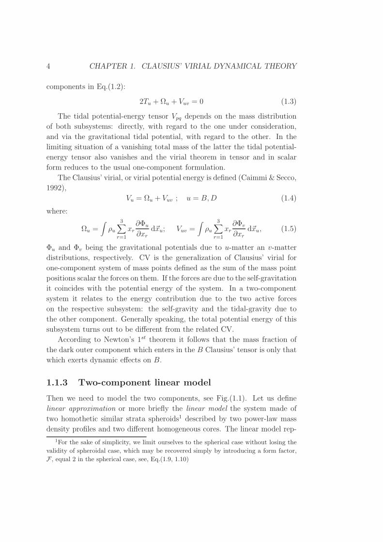
Figure 1.1: A two-components model where a homeoidally striated baryonic
component (B) is embedded within a homeoidally striated dark matter halo
(D). The DM isopycnic (i.e., constant density) surface tangent to the B
component at the top major axis, is denoted as Σ∗. The homeoid bounded
by Σ∗ and the external surface of the D component, Σ, exerts no dynamical
action on B, owing to the Newton’s first theorem. In the special case where
B and D are, in turn, homothetic (as assumed in the text), Σ∗ coincides with
the external surface of the B component (Raffaele, 2003).
resents, to a good extent, a baryonic (stellar) component embedded within
a DM halo with smoothed density profiles, expressed as:
ρD =ρoD
1 +(
rroD
)d ; CD =aDroD
(1.6)
ρB =ρoB
1 +(
rroB
)b ; CB =aBroB
(1.7)
where CB and CD are the two concentrations of the two components. In
earlier models, roB and roD were the radii of the two different homogeneous
cores, which typically assumed one tenth of the virial radii, aB and aD,
6 CHAPTER 1. CLAUSIUS’ VIRIAL DYNAMICAL THEORY
respectively. Accordingly, the concentrations in the smoothed profiles both
become equal to ten. The density profiles defined by Eq.(1.6) and Eq.(1.7),
have the advantage that they may be considered as a generalization of pseudo-
isothermal profiles which, in turn, may be regarded as sub-cases of the more
general Zhao profiles when: γ = 0; β = α = b, d.
But a realistic elliptical model has to be: e.g., a stellar component with
a Hernquist (1990) (hereafter, Her) density profile and a dark halo with a
cored or cuspy NFW profile (that means, according to Eq.(1.1), respectively:
α = 1; β = 4; γ = 1; χ = 3 and α = 1; β = 3; γ = 0; χ = 3, for the cored
NFW, α = 1; β = 3; γ = 1; χ = 2, for the cuspy NFW) (as in Marmo, 2003,
where two homeoidally striated ellipsoids are considered).
Then, the problem of transfering the outputs obtained with two cored
powerlaw profiles (which also hold, to a good extent, for the models with
smoothed profiles Eq.(1.6,1.7)) to the more general class of models with Zhao
profiles given by Eq.(1.1), is still open, as we will see in the next chapter.
We aim to find an explanation to some scaling relations for elliptical
galaxies, which are essentially relationships among the exponents of the three
quantities:
• re = the effective radius;
• Ie =L
2πr2e= mean effective surface brightness within re;
• σo = the central projected velocity dispersion.
The advantage of a simple cored power-law model is that it is able to extract,
in a completely analytical way, a number of main correlations, highlighting
the interplay of the parameters. Moreover, this preliminary analysis may also
underline what are simply details in the model and what, on the contrary,
is strictly connected with the physical reason for the existence of a FP for
two-component virialized systems. That allows us to open the road for a
generalization of present results.
1.1.4 Special virial configuration
For the sake of simplicity, the outer component D is assumed as frozen; this
constraint will not essentially influence our results in order to determine the
main features of the dynamic evolution of ETGs (and of virialized structures
in general). The main reason for this assumption is that the masses of the
1.1. MAIN LINES OF CV THEORY 7
two components are not equal, the outer one being about ten times the inner
one. As a consequence, tidal influences acting from the inner to the outer one
is weaker than the reverse (e.g., Caimmi and Secco, 1992; Caimmi, 1994).
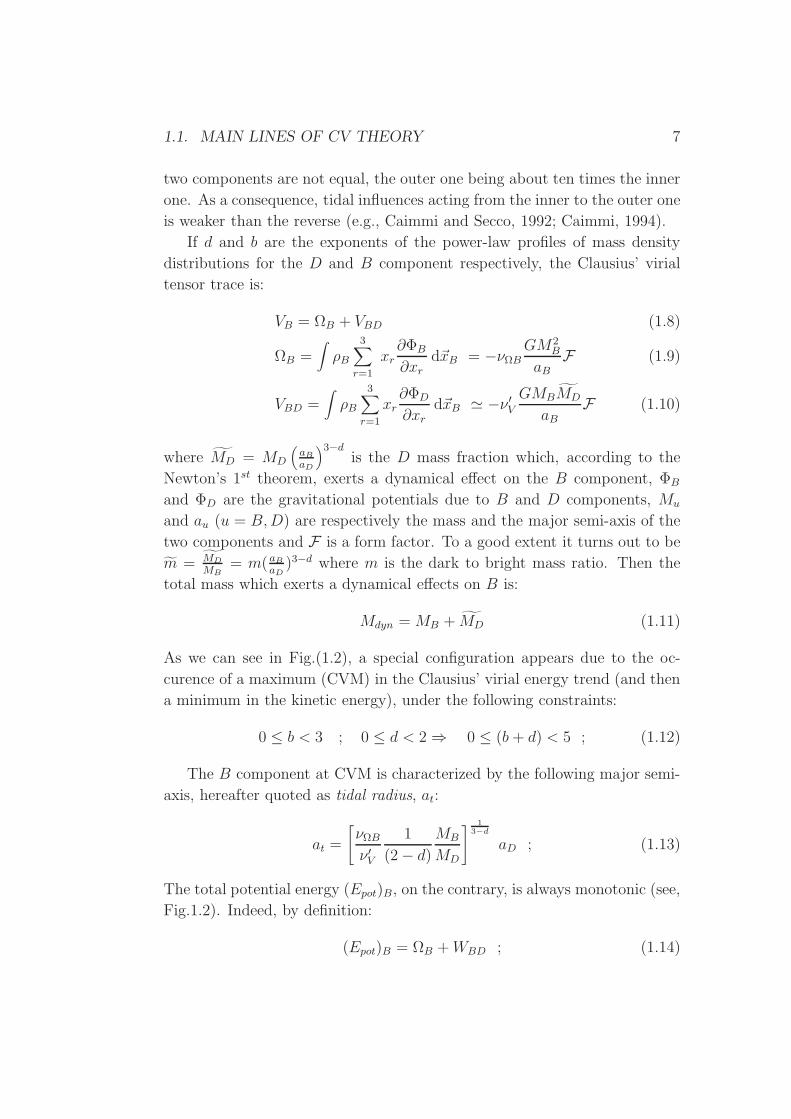
If d and b are the exponents of the power-law profiles of mass density
distributions for the D and B component respectively, the Clausius’ virial
tensor trace is:
VB = ΩB + VBD (1.8)
ΩB =∫ρB
3∑
r=1
xr
∂ΦB
∂xr
d~xB = −νΩB
GM2B
aBF (1.9)
VBD =∫
ρB3∑
r=1
xr
∂ΦD
∂xr
d~xB ≃ −ν ′
V
GMBMD
aBF (1.10)
where MD = MD
(aBaD
)3−dis the D mass fraction which, according to the
Newton’s 1st theorem, exerts a dynamical effect on the B component, ΦB
and ΦD are the gravitational potentials due to B and D components, Mu
and au (u = B,D) are respectively the mass and the major semi-axis of the
two components and F is a form factor. To a good extent it turns out to be
m = MD
MB= m(aB
aD)3−d where m is the dark to bright mass ratio. Then the
total mass which exerts a dynamical effects on B is:
Mdyn = MB + MD (1.11)
As we can see in Fig.(1.2), a special configuration appears due to the oc-
curence of a maximum (CVM) in the Clausius’ virial energy trend (and then
a minimum in the kinetic energy), under the following constraints:
0 ≤ b < 3 ; 0 ≤ d < 2 ⇒ 0 ≤ (b+ d) < 5 ; (1.12)
The B component at CVM is characterized by the following major semi-
axis, hereafter quoted as tidal radius, at:
at =
[νΩB
ν ′V
1
(2− d)
MB
MD
] 13−d
aD ; (1.13)
The total potential energy (Epot)B, on the contrary, is always monotonic (see,
Fig.1.2). Indeed, by definition:
(Epot)B = ΩB +WBD ; (1.14)
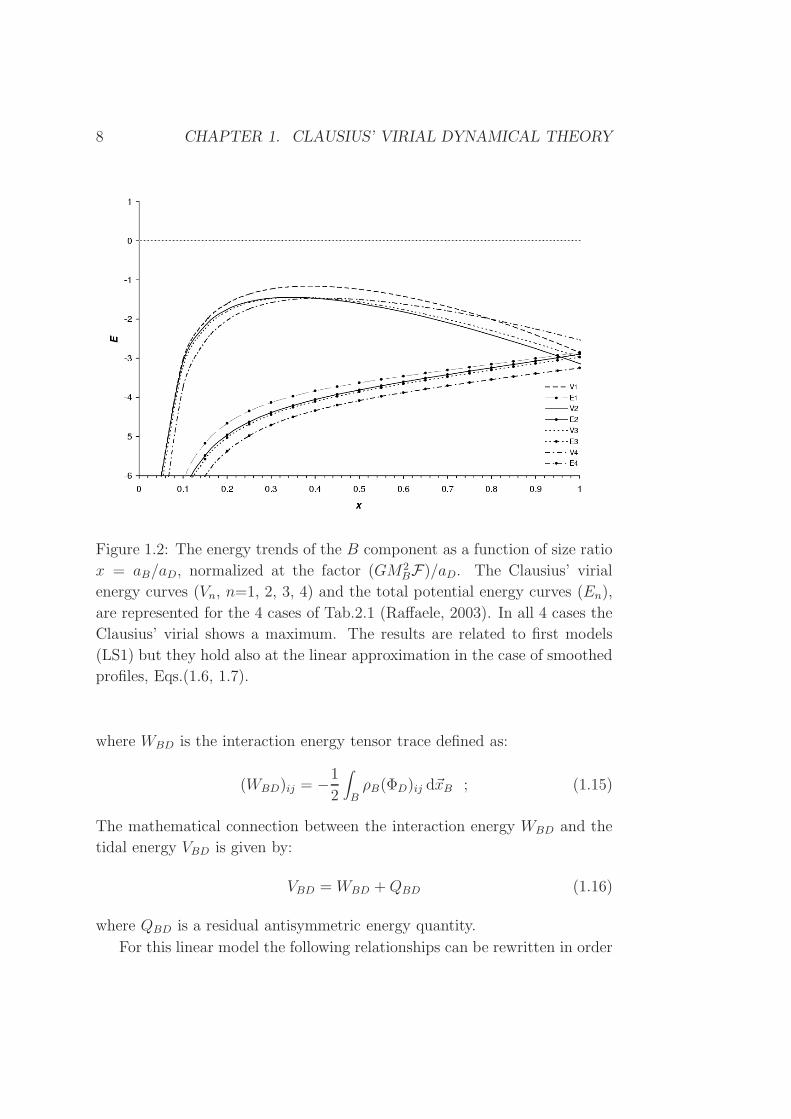
8 CHAPTER 1. CLAUSIUS’ VIRIAL DYNAMICAL THEORY
Figure 1.2: The energy trends of the B component as a function of size ratio
x = aB/aD, normalized at the factor (GM2BF)/aD. The Clausius’ virial
energy curves (Vn, n=1, 2, 3, 4) and the total potential energy curves (En),
are represented for the 4 cases of Tab.2.1 (Raffaele, 2003). In all 4 cases the
Clausius’ virial shows a maximum. The results are related to first models
(LS1) but they hold also at the linear approximation in the case of smoothed
profiles, Eqs.(1.6, 1.7).
where WBD is the interaction energy tensor trace defined as:
(WBD)ij = −1
2
∫
BρB(ΦD)ij d~xB ; (1.15)
The mathematical connection between the interaction energy WBD and the
tidal energy VBD is given by:
VBD = WBD +QBD (1.16)
where QBD is a residual antisymmetric energy quantity.
For this linear model the following relationships can be rewritten in order
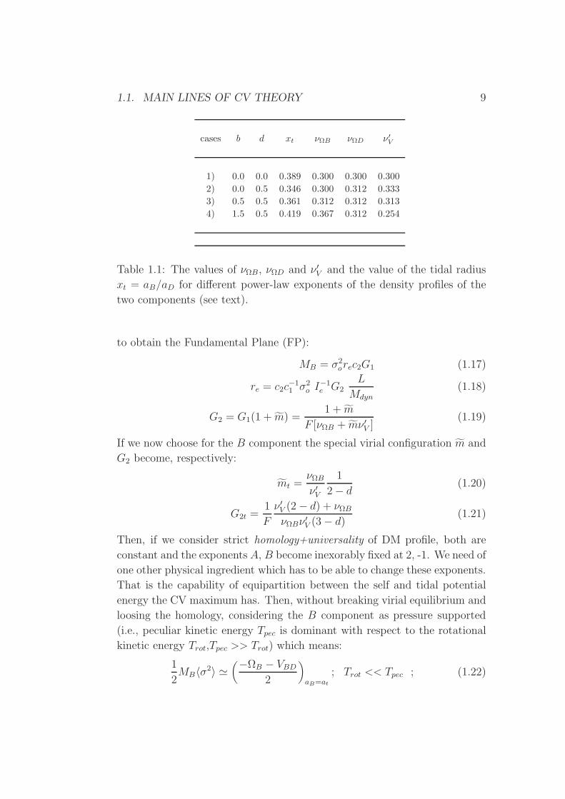
1.1. MAIN LINES OF CV THEORY 9
cases b d xt νΩB νΩD ν′
V
1) 0.0 0.0 0.389 0.300 0.300 0.300
2) 0.0 0.5 0.346 0.300 0.312 0.333
3) 0.5 0.5 0.361 0.312 0.312 0.313
4) 1.5 0.5 0.419 0.367 0.312 0.254
Table 1.1: The values of νΩB, νΩD and ν ′
V and the value of the tidal radius
xt = aB/aD for different power-law exponents of the density profiles of the
two components (see text).
to obtain the Fundamental Plane (FP):
MB = σ2orec2G1 (1.17)
re = c2c−11 σ2
o I−1e G2
L
Mdyn
(1.18)
G2 = G1(1 + m) =1 + m
F [νΩB + mν ′
V ](1.19)
If we now choose for the B component the special virial configuration m and
G2 become, respectively:
mt =νΩB
ν ′
V
1
2− d(1.20)
G2t =1
F
ν ′
V (2− d) + νΩB
νΩBν ′
V (3− d)(1.21)
Then, if we consider strict homology+universality of DM profile, both are
constant and the exponents A, B become inexorably fixed at 2, -1. We need of
one other physical ingredient which has to be able to change these exponents.
That is the capability of equipartition between the self and tidal potential
energy the CV maximum has. Then, without breaking virial equilibrium and
loosing the homology, considering the B component as pressure supported
(i.e., peculiar kinetic energy Tpec is dominant with respect to the rotational
kinetic energy Trot,Tpec >> Trot) which means:
1
2MB〈σ
2〉 ≃(−ΩB − VBD
2
)
aB=at
; Trot << Tpec ; (1.22)
10 CHAPTER 1. CLAUSIUS’ VIRIAL DYNAMICAL THEORY
(where 〈σ2〉 is the mean square velocity dispersion of the B component), at
the special configuration we obtain:
at ≃
12MB
σ2o
kva3−dD
ν ′
VGMBMDF
12−d
; (1.23)
The Eq.(1.6) yields the following FP:
re ∼ σ2
2−do a
3−d2−d
D m−1
2−dM−
12−d
B ; (1.24)
That means:
σAo = σ
22−do ;
IBe ∼ a3−d2−d
D m−1
2−dM−
12−d
B ;(1.25)
To share in almost equal amounts tidal potential and self potential energy
is the main property of the Clausius’ virial maximum. On this basis are
grounded all the main scale relations which the dynamical theory is able to
predict for ETGs. Indeed, from Eq.(1.25) we can derive all the outputs of
the theory as we will see in the next sections.
1.2 Mechanical arguments
The tidal radius configuration satisfies the d’Alembert principle of virtual
works and then it is an equilibrium configuration (see LS1). But due to the
fact that the total potential energy of the B component has not a minimum
(see, Fig.1.2), the equilibrium is unstable.
By definition, the work Ls done by the self gravity forces in order to
assemble the B-elements from infinity, is given by the self-potential energy
ΩB, while the work Lt done by the tidal gravity forces in order to put the
B component together with the D one from infinity through all the tidal
distortions, is given by the tidal potential energy VBD. Then a small variation
δVB for a small displacement δ~rB of all B points, when D is frozen (see LS5),
writes (see, Sec.(1.7)):
δVB ≃ δLs + δLt ; (1.26)
In other words if B contracts, less DM lies inside the Σ∗ surface and the
self gravity increases. The opposite occurs if B expands itself. Therefore,
even if both forces are attractive, the works for a virtual displacement are of
opposite signs (see LS5).
1.3. SCALING RELATIONS AT THE SPECIAL CONFIGURATION 11
1.3 Scaling relations at the special configura-
tion
The physical explanation for the main features of the FP for ETGs, and in
general for all virialized structures, is still an open question.
According to the dynamical theory here briefly explained the tilt can be
explained by assuming a strict homology which does not necessarily imply a
constant M/L ratio; the scale length induced on the gravitational baryonic
field by the DM halo distribution is the interpretation key.
Outputs vs. observables
The mechanical property of the tidal configuration to distribute in about
equal parts self and tidal energies, yields some outputs which are in good
agreement with observations.
From Eq.(1.25) we have:
A =2
2− d; (1.27)
and taking into account the two relationships which connect the FP coeffi-
cients A and B with the observed FP (Djorgovski & Santiago, 1993):
A = 2(1−αt)
1+αt;
B = − 11+αt
;(1.28)
we immediately obtain the tilt of the FP (M/L ∼ Mαt):
αt =1− d
3− d; (1.29)
and the other coefficient:
B = −3− d
2(2− d); (1.30)
as a function of the DM distribution. The surprising result is that the
quantities A, B, αt which define the FP and its tilt are independent of
m = MD/MB; this implies that the ETGs which belong to the FP may have
different fractions of baryonic to DM mass, but their DM density profile must
be the same.
12 CHAPTER 1. CLAUSIUS’ VIRIAL DYNAMICAL THEORY
A±∆A B±∆B Band
Dressler 1987 1.33± 0.05 −0.83± 0.03 B
Djorgovski & Davis 1987 1.39± 0.14 −0.90± 0.09 rGLucey et al. 1991 1.27± 0.07 −0.78± 0.09 V
Guzman et al. 1993 1.14± 0.07 −0.79± 0.07 V
Pahre et al. 1995 1.44± 0.04 −0.79± 0.03 K ′
Jørgensen et al. 1996 1.24± 0.07 −0.82± 0.02 r
Hudson et al. 1997 1.38± 0.04 −0.82± 0.03 R
Scodeggio et al. 1997 1.25± 0.02 −0.80± 0.02 I
Scodeggio 1997 1.55± 0.05 −0.80± 0.02 I
Pahre & Djorgovski 1997 1.66± 0.09 −0.75± 0.06 K ′
Pahre et al. 1998 1.53± 0.08 −0.80± 0.02 K
Kelson et al. 2000 1.31± 0.13 −0.86± 0.10 V
Gibbons et al. 2001 1.37± 0.04 −0.82± 0.01 R
Bernardi et al. 2003 1.49± 0.05 −0.75± 0.01 r
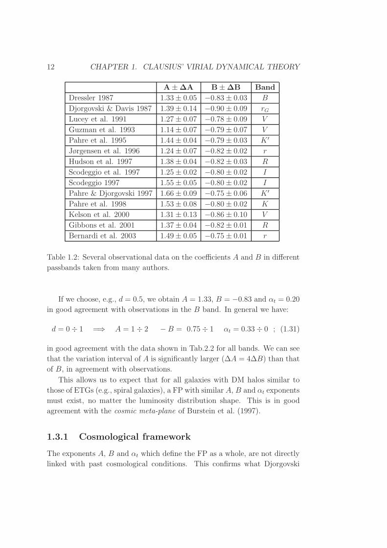
Table 1.2: Several observational data on the coefficients A and B in different
passbands taken from many authors.
If we choose, e.g., d = 0.5, we obtain A = 1.33, B = −0.83 and αt = 0.20
in good agreement with observations in the B band. In general we have:
d = 0÷ 1 =⇒ A = 1÷ 2 −B = 0.75÷ 1 αt = 0.33÷ 0 ; (1.31)
in good agreement with the data shown in Tab.2.2 for all bands. We can see
that the variation interval of A is significantly larger (∆A = 4∆B) than that
of B, in agreement with observations.
This allows us to expect that for all galaxies with DM halos similar to
those of ETGs (e.g., spiral galaxies), a FP with similar A, B and αt exponents
must exist, no matter the luminosity distribution shape. This is in good
agreement with the cosmic meta-plane of Burstein et al. (1997).
1.3.1 Cosmological framework
The exponents A, B and αt which define the FP as a whole, are not directly
linked with past cosmological conditions. This confirms what Djorgovski
1.3. SCALING RELATIONS AT THE SPECIAL CONFIGURATION 13
(1992) already noted for scaling relations in a CDM scenario. In fact, trans-
lating the exponents A and B in cosmological quantities, the FP condition
becomes:
2nrec + 10 = A(1− nrec)−B(12αt + 4nrec + 8) ; (1.32)
where nrec is the effective spectral index of perturbations at the recombi-
nation epoch. Combining this last equation with Eqs.(1.27, 1.29, 1.30) we
obtain an identity so that every information on nrec is lost. On the other
hand in the projections of the FP on the coordinate planes, the dependence
on the cosmological spectral index appears via the parameter γ′:
1
γ′(M)=
1 + 3αrec(M)
3=
5 + nrec
6; (1.33)
where, according to Gott & Rees (1975) and Coles & Lucchin (1995)(Chapts.
14, 15), αrec is the local slope of the CDMmass variance σ2M , at recombination
time trec, given by:
αrec = −d ln σM (trec)
d lnM; (1.34)
The dependence of the local slope αrec on the DM halo mass does not signif-
icantly change in the ΛCDM scenario (to be tested).
If the total energy is conserved from the maximum expansion phase to
virialization (with an energy re-distribution due to the violent relaxation
mechanism), the three main quantities of FP have the following dependences
on m and MB:
re ∼ mrMRB ; r =
(3− d)− γ′
γ′(3− d); R = 1/γ′ ; (1.35)
Ie ∼ miM IB ; I = i = 2
γ′ − (3− d)
γ′(3− d); (1.36)
σo ∼ msMSB ; s = −
1
2
(3− d)− γ′
γ′(3− d); S =
1
2
γ′ − 1
γ′; (1.37)
not only directly related to the DM distribution, via the exponent d, but also
to the perturbation spectrum via γ′.
It is now possible to write the FJ relation in general form:
L ∼ m2
(3−d)−γ′
(3−d)2(γ′−1) σ4γ′
(γ′−1)(3−d)o ; (1.38)
14 CHAPTER 1. CLAUSIUS’ VIRIAL DYNAMICAL THEORY
For a typical DM halo of MD ≃ 1011M⊙, we have γ′ ≃ 2 Gunn (1987), and
so we obtain:
L ∼ mj(d)σJ(d)o ; (1.39)
a result in surprising accordance with observational data, indeed:
d = 0÷ 1 =⇒
j = 0.44÷ 0
J = 2.7÷ 4
and for a value of d = 0.5 we obtain:
L ∼ m0.16σ3.2o (1.40)
The range results are in good agreement with Faber et al. (1989) (J = 2.61±
0.08 in B-band) and with the significantly steeper slope J = 4.14 ± 0.22 in
K-band by Pahre et al. (1998a). The theory predicts an intrinsic different
scatter in every FJ relationship due to the role of the factor mj (it is wider
as j increases, and disappears only when d = 1, i.e. αt = 0 so the tilt of the
FP disappears, see SubSec.(1.3.2)).
It is also interesting to note that 〈I〉e decreases as MB increases as soon
d < 1 (3− d > γ′); in fact we have:
L ∼ M0.8B ; re ∼ M0.5
B ⇒ 〈I〉e = L/2πr2e ∼ M−0.2B ; (1.41)
At the Clausius’ minimum configuration, the following holds:
(Mtot)at = MB
(1 +
νΩB
ν ′V (2− d)
); (1.42)
where (Mtot)at is the total mass Mtot at the tidal configuration at. If the
density profiles of B and D component are universal, the following also holds:
L/(Mtot)at ∼ L/MB ; (1.43)
so that the two ratios are simply proportional. Cappellari et al. (2006) found
M/L ∼ σ0.8o for an observed sample of either fast rotators or non-rotating
ETGs and S0 galaxies. In our approach, we obtain:
MB
L∼ m
αt(3−d)−γ′
(3−d)(γ′−1)σ2αtγ
′(MD)
γ′(MD)−1o ; (1.44)
1.3. SCALING RELATIONS AT THE SPECIAL CONFIGURATION 15
On the same DM scale we have an exponent 0.8 for σo and a negligible
dependence on m (being ∼ m0.04) in perfect agreement with Cappellari et
al. (2006) but also with Jørgensen (1999) value of 0.76 ± 0.08. At at the
following also holds:
log
(MD
Mtot
)
at
= − log
[1 +
ν ′
V
νΩB
(2− d)
]; (1.45)
meaning that(
MD
Mtot
)
at
only depends on the luminous and DM density pro-
files; if they are both universal for the galaxy family considered, this DM
fraction has to be the same for all members (i.e. not depending on m).
If the probable value for d is around 0.5 and b ranges from 2 ÷ 3 (e.g.,
Jaffe, 1983; Hernquist, 1990), we obtain log(Mtot
MB
)at
= 0.37 ÷ 0.69, where
log(Mtot
MB
)at= 0.50 at b = 2.5. The agreement with the histogram in Fig.5 of
Jørgensen (1999), related to ETGs in the central part of the Coma cluster
when the same IMF is assumed, appears to be very good.
1.3.2 About the tilt
In order to obtain a tilt of the FP we need to have a maximum in Clausius’
virial energy, that requires to have the equipartition between self and tidal
energy of the B component.
By considering the derivative of Clausius’ virial with respect to aB, with
the constraints given by Eq.(1.10)and Eq.(1.12), we conclude that theD mass
has to increase steeper than (aB/aD) in order to obtain the tilt. This means
that ρD has to decrease less than 1/r2 at the border of the B component, so
that tidal energy may overcome self energy from this border forwards. But
we can go further deducing a stricter constraint.
Let’s consider Eq.(1.36): 〈I〉e depends on the cosmological history of the
galaxies, on DM total mass and mass distribution and on the B component
mass. But the L/MB ratio (i.e., the FP tilt), is totally independent on the
cosmic perturbation spectra and on the mass ratiom and turns out to depend
only on the DM density profile. In fact, being:
L ∼ IeRe2 =⇒∼ mi+2rM I+2R
B (1.46)
16 CHAPTER 1. CLAUSIUS’ VIRIAL DYNAMICAL THEORY
we have:L
MB
∼ mi+2rM I+2R−1B (1.47)
where the exponent i + 2r = 0 shows the lost connection of the tilt with m
and the exponent I + 2R = 2/(3 − d) shows the lost connection of the tilt
with cosmology (trough γ′).
Moreover in order to have a positive tilt (as observed), we need:
2/(3− d) < 1 =⇒ 0 < d < 1 ; (1.48)
Therefore, the slope of the FP tells us a constraint on the density dis-
tribution of DM halos. To have a positive tilt we need the DM mass to
increase steeper than (aB/aD)2 at the border of the B mass; this means, in
turn, that ρD has to decrease less than 1/r.
1.4 Transition toward virialization
How the special configuration caracterized by the CV maximum may be
reached, during the stellar system evolution? The answer is strictly connected
with the problem of the end state of the collisionless stellar system after a
violent relaxation phase (Lynden-Bell, 1967; van Albada, 1982; Binney &
Tremaine, 1987 (Chapter 4); Burkert, 1994; White, 1996) and then to the
problem of the constraints under which this phase occurs (Merritt, 1999). In
consequence of this mechanism the proto-structure undergoes a sequence of
contractions and expansions during which Landau damping ensures the build-
up of a gradually increasing random kinetic energy due to the conversion of
radial ordered velocity into a dispersion velocity field (see, e.g., Huss et al.,
1999). But due to the virial equation, maximum of CV means minimum of
the macroscopic pressure (that is minimum value of TB), the stellar system
needs in order to virialize. This makes stronger the idea to look at this
special configuration as the best candidate for the initial virial stage because
it has the least requests for sustaining the structure in virial equilibrium and
it could also justify why the ellipticals are not completely relaxed systems
in respect to the collisionless dark halo, the problem adressed by White &
Narayan (1987). Moreover, the thermodynamical approach may help us to
understand when and why the stellar system choose to virialize on the CV
maximum.
1.5. THE THERMODYNAMICAL LINEAR APPROACH 17
1.5 The thermodynamical linear approach
Since Lynden-Bell (1967) first attempt to derive a statistical theory according
to the Vlasov equation, the thermal equilibrium in collisionless systems after
violent relaxation is still an open problem.
1.5.1 The temperature problem
We will enter deeply in this very complicate matter in the next chapter. Here
we limit ourselves to adress the problem as follows:
1. the time derivative of the gravitational potential, which is the engine
of the violent relaxation mechanism, is proportional to the energy per
unit mass of a system’s star (Binney & Tremaine, Chap.4, 1987);
2. to avoid the segregation of mass, not observed in ellipticals, we have
to remove the velocity dispersion problem when a collisionless system
of different mass populations is considered. Actually, in the Lynden-
Bell statistics the equilibrium distribution becomes a superposition of
Gaussian components with different velocity dispersion in the non-
degenerate limit;
3. after the Shu (1978) approach and the statistical attempts of Kull et al.
(1997), the problem has been resolved by Nakamura (2000). At fixed
value for mass, energy and phase-space volume of the system, Naka-
mura obtains a single Gaussian distribution for the equilibrium state
as soon as a smooth initial fine-grained distribution function (DF) is
assumed. Then the same mean dispersion velocity < σ2 > has to
characterize the different mass populations. That means also the same
energy per unit mass regardless from the stellar mass considered ac-
cording to the typical relaxation process whith no mass segregation
(item 1);
4. we will assume as an Ansatz partially justified by Nakamura’s result
(Nakamura, 2000) that for each stellar virial configuration of the B
system a mean temperature is given by:
T S =m∗ < σ2 >
k(1.49)
18 CHAPTER 1. CLAUSIUS’ VIRIAL DYNAMICAL THEORY
wherem∗ is the mean mass of the stars and k is the Boltzmann constant
(see, e.g., Lima Neto et al. 1999; Bertin & Trenti, 2003).
1.5.2 Thermodynamic information
The knowledge of the mean temperature allows us to take into account the
thermodynamic information, according to Layzer (1976):
I = Smax − S (1.50)
where Smax means the maximum value the entropy of the system may have
as soon as the constraints of it, which fix the actual value of its entropy to S,
are relaxed. According to the IIo Thermodynamic Principle it means that
the state with I → 0 is the natural attractor for a system.
Assuming as reference the entropy value which corresponds to the state
of maximum possible volume for B (x = 1), we are able to compare how
changes the information at each configuration x relative to this state:
I(x) = I(1)−V(x) (1.51)
S(x)− S(1) = V(x) (1.52)
Actually, we may move from the state x = 1 to the general state x by
a virtual sequence of thermodynamical quasi-static infinitesimal transforma-
tions (associated to an infinitesimal contraction ∆aB < 0) where the internal
energy of the B component is identified with the dominant peculiar kinetic
energy of the stars, TB, (which produces the macroscopic pressure of the B
subsystem) and the virial equilibrium is rearranged at each step (LS5). Un-
der the assumption of a frozen dark component, the variation of the work
done against the pressure by both the active forces on the B system, self-
and DM-gravity, is given by ∆VB according to the result of Sec.(1.7). Then
the heat variation ∆Q the structure is able to exchange with the surrounding
medium is:
∆Q =1
2∆VB (1.53)
In turn, TB ≃ 12Nm∗ < σ2 >, then the mean temperature (1.49) becomes:
T S =−VB
Nk(1.54)
N being the star number. Then virial equilibrium yields that the variation
of the internal energy of the B system, ∆TB, during the transition between
1.5. THE THERMODYNAMICAL LINEAR APPROACH 19
two virial states due to a small contraction, ∆x, goes: one half to increase
the mean temperature of B, ∆T S ∼ −12∆VB, the other half has to be lost
by radiation outwards (Eq.(1.53)). The result is formally the classical one
found by Chandrasekhar (1939) and Schwarzschild (1958) for a single gaseous
component with the microscopic internal energy due to the molecular motion.
But now, the variation of CV energy which gives the work done by both the
gravitational forces actives on the B system, is a non-monotonic function of
x (Fig.1.2).
As pointed out in LS5 in this last case we cannot reach equipartition
starting from x = 1 by a simple contraction of the system considered as
isolated but we need of a supplement of heat source without which the CVM
configuration is missed.
The entropy (normalized to the factor Nk/2) of the B system at x in
respect to that at x = 1 , is given by (LS5):
S(x)− S(1) = lnVB(1)
VB(x)= Vn(x) (1.55)
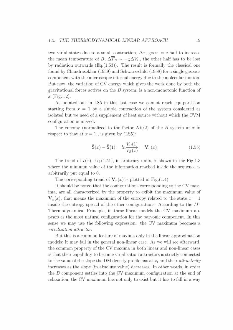
The trend of I(x), Eq.(1.51), in arbitrary units, is shown in the Fig.1.3
where the minimun value of the information reached inside the sequence is
arbitrarily put equal to 0.
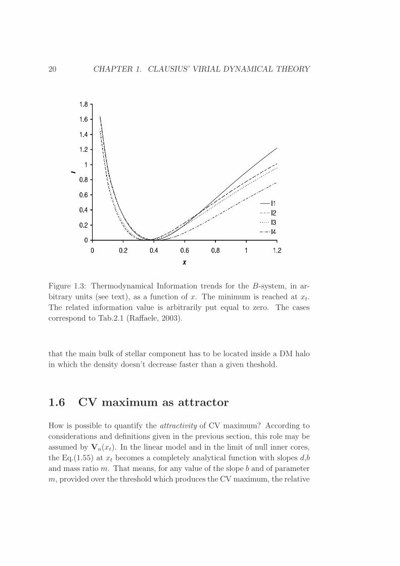
The corresponding trend of Vn(x) is plotted in Fig.(1.4)
It should be noted that the configurations corresponding to the CV max-
ima, are all characterized by the property to exibit the maximum value of
Vn(x), that means the maximum of the entropy related to the state x = 1
inside the entropy spread of the other configurations. According to the IIo
Thermodynamical Principle, in these linear models the CV maximum ap-
pears as the most natural configuration for the baryonic component. In this
sense we may use the following expression: the CV maximum becomes a
virialization attractor.
But this is a common feature of maxima only in the linear approximation
models; it may fail in the general non-linear case. As we will see afterward,
the common property of the CV maxima in both linear and non-linear cases
is that their capability to become virialization attractors is strictly connected
to the value of the slope the DM density profile has at xt and their attractivity
increases as the slope (in absolute value) decreases. In other words, in order
the B component settles into the CV maximum configuration at the end of
relaxation, the CV maximum has not only to exist but it has to fall in a way
20 CHAPTER 1. CLAUSIUS’ VIRIAL DYNAMICAL THEORY
Figure 1.3: Thermodynamical Information trends for the B-system, in ar-
bitrary units (see text), as a function of x. The minimum is reached at xt.
The related information value is arbitrarily put equal to zero. The cases
correspond to Tab.2.1 (Raffaele, 2003).
that the main bulk of stellar component has to be located inside a DM halo
in which the density doesn’t decrease faster than a given theshold.
1.6 CV maximum as attractor
How is possible to quantify the attractivity of CV maximum? According to
considerations and definitions given in the previous section, this role may be
assumed by Vn(xt). In the linear model and in the limit of null inner cores,
the Eq.(1.55) at xt becomes a completely analytical function with slopes d,b
and mass ratio m. That means, for any value of the slope b and of parameter
m, provided over the threshold which produces the CV maximum, the relative
1.6. CV MAXIMUM AS ATTRACTOR 21
Figure 1.4: Trends of the entropy function Vn(x) (eq.(1.55)) for the B-
system, in arbitrary units (see text), as function of x. The cases are corre-
sponding to Tab.2.1. The maxima occur at the tidal radii (Raffaele, 2003).
entropy at xt is:
S(xt)− S(1) = lnVB(1)
VB(xt)= Vn(xt, b, d,m); (1.56)
which exhibits the following features.
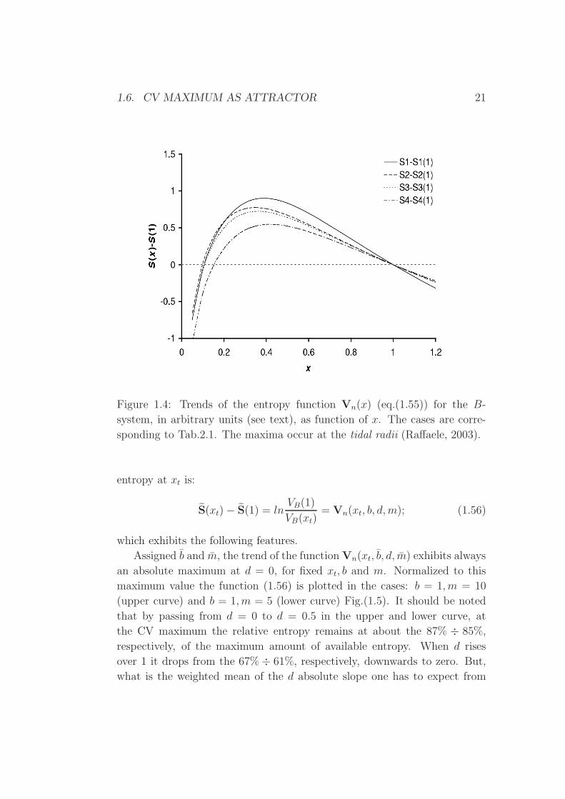
Assigned b and m, the trend of the functionVn(xt, b, d, m) exhibits always
an absolute maximum at d = 0, for fixed xt, b and m. Normalized to this
maximum value the function (1.56) is plotted in the cases: b = 1, m = 10
(upper curve) and b = 1, m = 5 (lower curve) Fig.(1.5). It should be noted
that by passing from d = 0 to d = 0.5 in the upper and lower curve, at
the CV maximum the relative entropy remains at about the 87% ÷ 85%,
respectively, of the maximum amount of available entropy. When d rises
over 1 it drops from the 67% ÷ 61%, respectively, downwards to zero. But,
what is the weighted mean of the d absolute slope one has to expect from
22 CHAPTER 1. CLAUSIUS’ VIRIAL DYNAMICAL THEORY
Figure 1.5: Trend of the function Vn(xt, b, d, m) normalized to its maximum
value at d = 0 (Eq.(1.57)) in the cases: b = 1, m = 10 (upper curve) and
b = 1 ,m = 5 (lower curve).
the distribution of Fig.(1.5)? If we perform the weighted mean dwm given to
each value of d as weight the corresponding value of the normalized function:
Vn(xt, b, d, m) = Vn(xt, b, d, m)/Vn(xt, b, d = 0, m) (1.57)
That means:
dwm =
∫d · Vn(xt, b, d, m) dd∫Vn(xt, b, d, m) dd
(1.58)
It is noteworthy that it results to be, dwm = 0.4681, in the case m = 10
and dwm = 0.4618 in the case m = 5. That gives deep meaning at the value
1.7. SMALL DEPARTURES FROM VIRIAL EQUILIBRIUM 23
d = 0.5 used in the whole linear theory in order to match the theory with
many FP observations.
The general message which comes from Fig.1.5 is that in order to increase
the attractivity of a CV maximum, expressed by Eq.(1.56), we need to de-
crease the slope at which the maximum falls. We will come back to this
conspiracy between the attractivity and the slope in the non-linear thermo-
dynamical approach considered in the chapt.6.
1.7 Small departures from virial equilibrium
We will consider now what is the mathematical form of the VB potential
energy variation as soon as the B inner system contracts or expands its
initial volume So of a small quantity ∆So. Following Chandrasekhar’s anal-
ysis (Chandrasekhar, 1969, Chapter 2): by definition the Clausius virial is
a global, integral parameter of an extrinsic attribute, that means of a quan-
tity which is not intrinsic to the fluid element (like pressure or density) but
something, we name F (~x), which it assumes simply by virtue of its location
as the gravitational potential and its first derivative are. Then the variation
of the integral:
δ∫
So
ρBF d~xB =∫
So+∆So
ρBF d~xB −∫
So
ρBF d~xB (1.59)
when fluid volume changes from So to So +∆So by subjecting its boundary
to the displacement ~ξ(~x, t) = ~x − ~xo, may be transformed into the integral
over the unperturbed volume, that is:
δ∫
So
ρBF d~xB =∫
So
ρB∆F d~xB (1.60)
where ∆F is the Lagrangian change in F consequent to the displacement ~ξ.
The extension of this analysis to two-component systems has been per-
formed with the following result:
δΩB = −∫
So
ρB3∑
r=1
ξr∂ΦB
∂xr
d~xB(1.61)
δVBD = −∫
So
ρB3∑
k=1
3∑
r=1
ξk∂
∂xk
(xr
∂ΦD
∂xr
) d~xB −∫
Mo
ρD3∑
r=1
ξ′r∂ΦB
∂xr
d~xD
+∫
Mo
ρD3∑
k=1
3∑
r=1
ξ′k∂
∂xk
(xr
∂ΦB
∂xr
) d~xD(1.62)
24 CHAPTER 1. CLAUSIUS’ VIRIAL DYNAMICAL THEORY
where the unperturbed volume of D-component is Mo and ~ξ′ is the amount
of the perturbation in the point domain of the same component.
Under the assumption of a frozen dark component, ~ξ′ turns out to vanish
and Eq.(1.62) reduces to:
δVBD ≃ δLs + δLt ≃ −∫
So
ρB3∑
r=1
ξr∂ΦB
∂xr
d~xB
−∫
So
ρB3∑
k=1
3∑
r=1
ξk∂
∂xk
(xr
∂ΦD
∂xr
) d~xB = (δVB)aD (1.63)
By definition of tidal radius, which is the B dimension at the maximum
of its Clausius virial energy, at frozen aD, the (δVB)aD is stationary at at(Fig.1.2)(see, LS1); then by moving of a virtual2 displacement δaB, from
aB = at, we have:
δLs + δLt ≃ (δVB(at))aD = 0 (1.64)
This means the configuration at at satisfies the d’Alembert Principle of the
virtual works (see also LS1). The physical reason is the following: if, e.g.,
B contracts, less dark matter enters inside the SB surface, in the meanwhile
the self gravity increases. The opposite occurs if B expands itself. Then,
even if both forces are attractive, the works which correspond to them, for a
virtual displacement, are of opposite signs (see, LS1). Then the tidal radius
configuration is an equilibrium configuration even if not stable because the
total potential energy of B has not a minimum (Fig.1.2).
2Here virtual means at frozen D.
Bibliography
Arad, I., Dekel, A., Klypin, A. A.,2004. MNRAS, 353, 15.
Arad, I., & Lynden-Bell, D., 2005. MNRAS, 361, 385.
Ascasibar, Y., Yepes, G., Gottlober, S., Muller, V., 2004. MNRAS, 352, 1109.
Babcock, H.W., 1939. LicOB., 19, 41.
Bender, R., Burstein, D., Faber, S.M., 1992. ApJ, 399, 462.
Bernardi, M., Sheth, R.K., Annis, J., and 28 coauthors, 2003a. AJ, 125, 1849.
Bernardi, M., Sheth, R.K., Annis, J., and 28 coauthors, 2003b. AJ, 125, 1866.
Bertin, G., Trenti, M., 2003. ApJ, 584, 729.
Bindoni, D., 2005. Master Thesis, Universit di Padova, Italy.
Bindoni, D., Secco, L., Caimmi, R., D’Onofrio, M., Valentinuzzi, T., 2007. IAUS,
235, 79.
Bindoni, D., Secco, L., Caimmi, R., D’Onofrio, M., 2007. ASPC, 374, 489.
Bindoni, D., Secco, L., 2008. NewAR, 52, 1B.
Binney, J., 1978. MNRAS, 183, 501.
Binney J., Tremaine S., 1987. Galactic Dynamics, Princeton, NJ, Princeton Uni-
versity Press.
Binney, J., Gerhard, O., Spergel, D., 1997. MNRAS, 288, 365.
Binney, J., Merrifield, M., 1998. Galactic Astronomy, Princeton, NJ, Princeton
University Press.
Binney, J.J., Evans, N.W., 2001. MNRAS, 327, L27.
25
26 BIBLIOGRAPHY
Bindoni, D., 2005. Master Thesis, Universit di Padova, Italy.
Blais-Ouellette, S., Carignan, C., Amram, P., Ct, S., 1999. AJ, 118, 2123.
Blais-Ouellette, S., Amram, P., Carignan, C., Swaters, R., 2004. A&A, 420, 147.
Bosma, A., 1978. IAUS, 77, 28.
Bosma, A., 1981. AJ, 86, 1825.
Brosche, P., Caimmi, R., Secco, L., 1983. A&A, 125, 338.
Buote, D., 2004. IAUS, 220, 149.
Burkert, A., 1993. A&A, 278, 23.
Burkert, A., 1995. ApJ, 447, L25.
Burstein, D., Bender, R., Faber, S.M., Nolthenius, R., 1997 ApJ, 114, 1365.
Caimmi, R., Secco, L., Brosche, P., 1984. A&A, 139, 411.
Caimmi, R., Secco, L., 1992. ApJ, 395, 119.
Caimmi, R., 1993. ApJ, 419, 615.
Caimmi, R., 1994. Astrophysics & Space Sci., 219, 49.
Caimmi, R., Marmo, C., 2003. NewA, 8, 119.
Caimmi, R., 2004. AN, 325, 326.
Cappellari, M., Bacon, R., Bureau, M., Damen, M.C., Davies, R.L., de Zeeuw,
P.T. and 9 cohautors, 2006. MNRAS, 366, 1126.
Carignan, C., Beaulieu, S., 1989. ApJ, 347, 760.
Chandrasekhar, S., 1939. Stellar Structure, Dover, New York.
Chandrasekhar, S., 1969. Ellipsoidal figures of equilibrium (New Haven: Yale Univ.
Press).
Chavanis, P. H., 2002. astro.ph., 12205.
Ciotti, L., Lanzoni, B., Renzini, A., 1996. MNRAS, 282, 1.
Ciotti, L., 1999, ApJ, 520, 574.
BIBLIOGRAPHY 27
Cole, S., Lacey, C., 1996. MNRAS, 281, 716.
Coles, P., Lucchin, F., 1995. Wiley Edition.
Colın, P., Klypin, A., Valenzuela, O., Gottlober, S., 2004. ApJ, 612, 50.
Combes, F., Boisse’, P., Mazure, A., Blanchard, A., 1995. Galaxies and Cosmology,
ed. Springer.
Cote, S., Carignan, C., Sancisi, R., 1991. AJ, 102, 904.
Dalcanton, J. J., Hogan, C. J., 2001. ApJ, 561, 35.
Dantas, C.C., Ribeiro, A.L.B., Capelato, H.V., de Carvalho R.R., 2000. ApJ, 528,
L5.
Debattista, V.P., Sellwood, J.A., 2000. ApJ, 543, 704.
Debattista, V.P., Gerhard, O., Sevenster, M.N., 2002. MNRAS, 334, 355.
de Blok, W.J.G., McGaugh, S.S., 1997. MNRAS, 290, 533.
de Blok, W.J.G., McGaugh, S., Rubin, V.C., 2001. AJ, 122, 2396.
de Blok, W.J.G., Bosma, A., McGaugh, S., 2003. MNRAS, 340, 657.
Dehnen, W., McLaughlin, D. E., 2005. MNRAS, 363, 1057.
Dekel, A., Devor, J., Arad, I., 2002. ASPC, 283, 307.
Dolag, K., Bartelmann, M., Perrotta, F., Baccigalupi, C., Moscardini, L.,
Meheghetti, M., Tormen, G., 2004. A&AS, 416, 853.
D’Onofrio, M., Valentinuzzi, T., Secco, L., Caimmi, R., Bindoni, D., 2006. NewAR,
50, 447.
Djorgovski, S. 1985, PASP, 97, 1119.
Djorgovski, S.G., Davis M., 1987. ApJ, 313, 59.
Djorgovski, S.G., 1992. ed. G.Longo et al. (Kluver Accademin Pub., Netherlands),
337-356.
Djorgovski, S.G., Santiago, B.X., 1993, ed.Danziger I.J. et al., ESO, Garching, pg.
59.
28 BIBLIOGRAPHY
Djorgovski, S.G., 1995, ApJ, 438,L29.
Dressler, A., Lynden-Bell, D., Burstein, D., Davies, R.L., Faber, S.M., Terlevich,
R., Wegner, G., 1987. ApJ, 313, 42.
Dubinski, J., 1994. ApJ, 431, 617.
Efthymiopoulos, C., Voglis, N., & Kalapotharakos, C., 2006. astro.ph., 10246.
Englmaier, P., Gerhard, O.E., 1999. MNRAS, 304, 512.
Faber, S.M., Wegner, G., Burstein, D., Davies, R., Dressler, A., Lynden-Bell, D.,
Terlevich, R.J., 1989. AJ, Sup.Ser.69,763-808.
Flores, R.A., Primack, J.R., 1994. ApJ, 427, 1.
Fukushige, T., Makino, J., 1997. ApJ, 477, L9.
Fukushige, T., Makino, J., 2001. ApJ, 557, 533.
Garrido, O., 2003. PhD Thesis, Universit de Provence, France.
Garrido, O., Amram, P., Carignan, C., Blais-Ouellette, S., Marcelin, M., Russeil,
D., 2004. IAUS, 220, 327.
Garrido, O., Marcelin, M., Amram, P., Balkowski, C., Gach, J.L., Boulesteix, J.,
2005. MNRAS, 362, 127.
Gentile, G., Salucci, P., Klein, U., Vergani, D., Kalberla, P., 2004. MNRAS, 351,
903.
Gibbons, R.A., Fruchter, A.S., Bothun, G.D., 2001. AJ, 121, 649.
Gott, J.R., Rees, M., 1975. A&A, 45, 365.
Graham, A.W., Merritt, D., Moore, B., Diemand, J., Terzic, B., 2006. AJ, 132,
2701.
Gunn, J.E., Gott, J.R.III, 1972. ApJ, 176, 1.
Gunn, G.E., 1987. NATO ASI Ser.C207, Reidel Publ. Co., Dordrecht, Holland,
413.
Guzman, R., Lucey, J.R., Bower, R.G., 1993. MNRAS, 265, 731.
Hansen, S.H., 2004. MNRAS, 352, L41.
BIBLIOGRAPHY 29
Hartwick, F. D. A., 2007. ApJ, submitted, arXiv:0711.0466.
Hayashi E., Navarro, J.F., Power, C., Jenkins, A., Frenk, C.S., White, S.D.M.,
Springel, V., Stadel, J., Quinn, T.R., 2004. MNRAS, 355, 794.
Hernquist, L., 1990. ApJ, 356, 359.
von Hoerner, V.S., 1958. ZA, 44, 221.
Horowitz, G., Katz, J.B., 1978. ApJ, 222, 94.
Hudson, M.J., Lucey, J.R., Smith, R.J., Steel, J., 1997. MNRAS, 291, 488.
Huss, A., Jain, B., Steinmetz, M., 1999. ApJ, 517, 64.
Ibata, R., Lewis, G.F., Irwin, M., Totten, E., Quinn, T., 2001. ApJ, 551, 294.
Jaffe, W., 1983, MNRAS, 202, 995.
Jaynes, E. T., 1957a. Phys. Rev., 106, 620.
Jaynes, E. T., 1957b. Phys. Rev., 108, 171.
Jaynes, E. T., 1983. Paper on Probability, Statistics, and Statistical Physics (Dor-
drecht: Reidel).
Jeans, J., 1915. MNRAS, 76, 70.
Jørgensen, I., Franx, M., Kjærgaard, P., 1996. MNRAS, 280, 167.
Jørgensen, I., 1999. MNRAS, 306, 607.
Kelson, D.D., Illingworth, G.D., van Dokkum, Franx, M., 2000. ApJ, 531, 184.
King, I., 1962. AJ, 67, 471.
King, I.R., 1966, AJ, 71(1), 64.
Kerr, F.J., Lynden-Bell, D., 1986. MNRAS, 221, 1023.
Klar, J.S., Mucket, J.P., 2008. A&A, 486, 25K.
Klypin, A., Zhao, H.S., Somerville, R.S., 2002. ApJ, 573, 597.
Kormendy J., Djorgovski S., 1989. Annu.Rev.Astron.Astrophys, 27, 235.
Kravtsov, A.V., Klypin, A.A., Bullock, J.S., Primack, J.R., 1998. ApJ, 502, 48.
30 BIBLIOGRAPHY
Kuijken, K., Gimlore, G., 1991. ApJ, 367, L9.
Kull, A, Treumann, R.A., Boehringer, H., 1997. ApJ, 484, 58.
Kuzio de Naray, R., McGaugh, S.S., de Blok, W.J.G., Bosma, A., 2006. ApJS,
165, 461.
Lacey, C., Cole, S., 1993. MNRAS, 262, 627L.
Layzer, D., 1976. ApJ, 206, 559.
Lima Neto, G.B., Gerbal, D., Marquez, I., 1999. MNRAS, 309, 481.
Limber, D.N., 1959. ApJ, 130, 414.
Longair, M., 1984. Theoretical Concepts in Physics (Cambridge: Univ. Press).
Lubin, L. M., & Bahcall, N. A., 1993. ApJ, 415, L17.
Lucey, J.R., Bower, R.G., Ellis, R.S., 1991. MNRAS, 249, 755.
Lynden-Bell, D., 1967. MNRAS, 136, 101.
Lynden-Bell, D., Wood, R., 1968. MNRAS, 138, 415.
Madsen, J., 1987. ApJ, 316, 497.
Mahdavi, A., Geller, M.J., 2004. ApJ, 607, 202.
Majewski, S.R., Law, D.R., Johnston, K.V., Skrutskie, M.F., Weinberg, M.D.,
2004. IAUS, 220, 189.
Marchesini, D., D’Onghia, E., Chincarini, G., Firmani, C., Conconi, P., Molinari,
E., Zacchei, A., 2002. ApJ, 575, 801.
Marmo, C., 2003. PhD Thesis, University of Padua, Italy.
Marquez, I., Lima Neto, G.B., Capelato, H., Durret, F., Lanzoni, B., Gerbal, D.,
2001. A&A, 379, 767.
Merrifield, M. R., 2004. IAUS, 220, 431.
Merritt, D., 1999. PASP, 111, 129.
Merritt, D., Navarro, J.F., Ludlow, A., Jenkins, A., 2005. ApJ, 624, 85.
McGaugh, S.S., de Blok, W.J.G., 1998.ApJ, 499, 41.

BIBLIOGRAPHY 31
McGaugh, S.S., Rubin, V.C., de Blok, W.J.G., 2001. AJ, 122, 2381.
Monet, D.G., Schechter, P.L., Richstone, D.O., 1981. ApJ, 245, 454.
Moore, B., 1994. Natur., 370, 629.
Moore, B., Governato, F., Quinn, T., Stadel, J., Lake G., Tozzi P., 1998. ApJ,
499, L5.
Moore, B., Ghigna, S., Governato, F., Lake, G., Quinn, T., Stadel, J., Tozzi, P.,
1999. ApJ, 524, 19.
Mucket, J. P., Hoeft, M., 2003. A&A, 404, 809.
Nakamura, T.K., 2000. ApJ, 531, 739.
Navarro, J.F., Frenk, C.S., White, S.D.M., 1996. ApJ, 462, 563.
Navarro, J.F., Frenk, C.S., White, S.D.M., 1997. ApJ, 490, 493.
Navarro, J.F., Hayashi, E., Power, C., Jenkins, A.R., Frenk, C.S., White, S.D.M.,
Springel, V., Stadel, J., Quinn, T.R., 2004. MNRAS, 349, 1039.
Oemler, A.Jr., 1976. ApJ, 209, 693.
Ogorodnikov, K. F., 1965. Dynamics of Stellar System (Oxford: Pergamon Press).
Olling, R.P., Merrifield, M.R., 2000. MNRAS, 311, 361.
Olling, R.P., Merrifield, M.R., 2001. MNRAS, 326, 164.
Pahre, M.A., Djorgovski, S.G., De Carvalho, R.R., 1995. ApJ, 453, 17.
Pahre, M.A., Djorgovski, S.G., 1997. ASPC, 116, 154.
Pahre, M.A., Djorgovski, S.G., De Carvalho, R.R., 1998a. AJ, 116, 1591.
Pahre, M.A., De Carvalho, R.R., Djorgovski, S.G., 1998b. AJ, 116, 1606.
Plummer, H.C., 1911. MNRAS, 71, 460.
Pointecouteau, E., Arnaud, M., Kaastra, J., de Plaa, J., 2004. A&A, 423, 33.
Power, C., Navarro, J.F., Jenkins, A., Frenk, C.S., White, S.D.M., Springel, V.,
Stadel, J., Quinn, T., 2003. MNRAS, 338, 14.
Raffaele, A., 2003. Master Thesis, University of Padua, Italy.
32 BIBLIOGRAPHY
Rasia, E., Tormen, G., Moscardini, L., 2004. MNRAS, 351, 237.
Reed, D., Gardner, J., Quinn, T., Stadel, J., Fardal, M., Lake, G., Governato, F.,
2003. MNRAS, 346, 565.
Rhee, G., Valenzuela, O., Klypin, A., Holtzman, J., Moorthy, B., 2004. ApJ, 617,
1059.
Ricotti, M., 2003. MNRAS, 334, 1237.
Roberts, P.H., 1962. ApJ 136, 1108.
Rubin, V.C., Thonnard, N., Ford, W.K.Jr., 1978. ApJ, 225, 107.
Sackett, P.D., Sparke, L.S., 1990. ApJ, 361, 408.
Salucci, P., 2001. MNRAS, 320, 1.
Sancisi, R., 2004. IUAS, 220, 233.
Sand, D.J., Treu, T., Smith, G.P., Ellis, R.S., 2004. ApJ, 604, 88.
Schwarzschild, M., 1958. Structure and Evolution of the Stars, Dover, New York.
Scodeggio, M., 1997. PhD Thesis.
Scodeggio, M., Giovanelli, R., Haynes, M.P., 1997. AJ, 113, 2087.
Secco, L., 2000. NewA, 5, 403.
Secco, L., 2001. NewA, 6, 339.
Secco, L., 2003. ASPC, 296, 87.
Secco, L., 2005. NewA, 10, 349.
Secco L., Caimmi R., D’Onofrio M., Bindoni D., 2007. ASPC, 374, 431.
Secco, L., Bindoni, D., 2009. NewA, submitted.
Sevenster, M.N., 1999. MNRAS, 310, 629.
Shannon, C. E., 1948. BSTJ, 27, 379 and 623.
Shu, F. H., 1969. ApJ, 158, 505.
Shu, F.H., 1978. ApJ, 225, 83.
BIBLIOGRAPHY 33
Shu, F. H., 1987. ApJ, 316, 502.
Silk, J., 1999. In: Formation of structure in the universe, Dekel, A., Ostriker, J.P.
(Eds), Cambridge University Press, p. 98.
Simon, J.D., Bolatto, A.D., Leroy, A., Blitz, L., 2003. ApJ, 596, 957.
Soaker, N., 1996. ApJ, 457, 287.
Spano, M., Marcelin, M., Amram, P., Carignan, C., Epinat, B., Hernandez, O.,
2008. MNRAS, 383, 297.
Spekkens K., Giovanelli R., Haynes, M.P., 2005. AJ, 129, 2119.
Spergel, D. N., & Hernquist, L., 1992., ApJ, 397, L75.
Spitzer, L., 1969. ApJ, 158, L139.
Stiavelli, M., 1987. MmSAI, 58, 477.
Stiavelli, M., & Bertin, G., 1987. MNRAS, 229, 61.
Stiavelli, M., & Sparke, L. S., 1991. ApJ, 382, 466.
Syer, D., White, S.D.M., 1998. MNRAS, 293, 337.
Swaters, R.A., 1999. Ph.D. Thesis, Rijksuniversiteit Groningen, Netherlands.
Swaters, R.A., Madore, B.F., Trewhella, M., 2000. ApJ, 531, 107.
Swaters, R.A., Madore, B.F., van den Bosch, F.C., Balcells, M., 2003a. ApJ, 583,
732.
Swaters, R.A., Verheijen, M.A.W., Bershady, M.A., Andersen, D.R., 2003b. ApJ,
587, L19.
Subramanian, K., Cen, R., Ostriker, J.P., 2000. ApJ, 538, 528.
Taylor, J.E., Navarro, J.F., 2001. ApJ, 563, 483.
Tormen, G., Bouchet, F.R., White, S.D.M., 1997. MNRAS, 286, 865.
Tremaine, S., Henon, M., & Lynden-Bell, D., 1986. MNRAS, 219, 285.
Valentinuzzi, T., 2006. PhD Thesis, University of Padova, Italy.
van Albada, T.S., 1982. MNRAS, 201, 939.
34 BIBLIOGRAPHY
van Albada, T.S., Bahcall, J.N., Begeman, K., Sancisi, R., 1985. ApJ, 295, 305.
van den Bosch, F.C., Robertson, B.E., Dalcanton, J.J., de Blok, W.J.G., 2000.
AJ, 119, 1579.
van den Bosch, F.C., Swaters, R.A., 2001. MNRAS, 325, 1017.
Vogelsberger, M., White, S. D. M., Helmi, A., Springel, V., 2007. MNRAS, sub-
mitted, arXiv:0711.1105.
Weiner, B.J., Sellwood, J.A., Williams, T.B., 2001. ApJ, 546, 931.
White, S.D.M., Narayan, N., 1987. MNRAS, 229, 103.
White, S.D.M., 1996. clss.conf., 349.
Zhao, H.S., 1996. MNRAS, 278, 488.
Zwicky, F., 1937. ApJ, 86, 217.


![Computation of planetary atmospheres by action mechanics ......Virial lapse rates Clausius’ virial theorem [6] states that the mean kinetic energy (+mv2/2) of particles in a gravitationally](https://img.dokumen.tips/doc/110x75/61125973acdc0a35b809178c/computation-of-planetary-atmospheres-by-action-mechanics-virial-lapse-rates.jpg)