Embed Size (px)
Citation preview

Classifier Combination for Biometrics

Voting Example (1)
Candidate A
Candidate B
Candidate C
Voter 1
Voter 2
Voter N
A
B
C
• Each candidate is a class.• Each voter is a classifier.• The voting problem is to define the type of voter’s output and to combine the results of the vote.

Voting Example (2)
Majority voting:
each voter can vote for one candidate; candidate with biggest number of votes wins.
Suppose:200 voters – A > C > B195 voters – B > C > A20 voters – C > B > A
Is C the worst candidate? Consider candidates in pairs:
C and A : 215 voters for C and 200 for AC and B : 220 voters for C and 195 for B

Voting Example (3)
Borda ( 18th century) count:Each voter gives to the first choice candidate 2 points, 1 point to second choice and 0 for third choice candidate.
In our example:A – 400 points, B – 410 and C – 435 points.
Approval voting :Each voter gives one point to every candidate he approves, and no points for others.

Voting Example (4)
• Additional modifications:• See http://en.wikipedia.org/wiki/Category:Voting_systems• Multi-stage votes• Confidence vote
• Main problem with defining voting methods:What is the ‘true class’ or ‘true candidate’ ?

Combination Problems
Classifiercombination
Other fusionapplication
(combining non-classifierexpert estimates – non-generic application problems)
Non-ensemblecombinations
ClassifierEnsembles
(large number of automatically generated classifiers of the same type)
Large number of classes
Small number of classes
(Easily solved by constructing a secondary classifier in a score space)
• Verification Problems• Identification Problems
• Biometric Applications• Handwriting Applications

Multi-Biometrics
� Single biometric may not be � Secure� Provide sufficient coverage� Accurate� Efficient
Fusion
Multiple Tokens
Multiple Modes
Multiple Matchers
Multiple Sensors
Multiple Fingers
Multiple Samples

Combination of biometric matchers
Fingerprint matching
Hand geometry matching
Signature matching
Alice Bob
:
2612 :
Alice Bob
:
0.310.45
:
Alice Bob
:
5.547.81
:
Alice Bob
:
0.950.11
:
Combination algorithm
• Criteria for classifier combination- performance on training/testing sets.• Classifiers can produce different types of scores – integers, floats

Types of classifiers and type conversion
• Combination methods usually accept input of one type.• If combined classifiers produce different type of input, then conversion is required.
Example of scores
Output
Type IIIType IIType I
Confidence scoresRanking
One class is chosen
S(C1)=.4S(C2)=.3
….S(Ck)=.05
…..S(Cn)=0
S(C1)=n-1S(C2)=n-2
….S(Ck)=n-k
…..S(Cn)=0
S(C1)=1S(C2)=0
….S(Ck)=0
…..S(Cn)=0

Combination algorithms
Combination algorithmsOutput values
Class ranking with confidencescore
Class ranking
The single class
Sum rule,Neural network.
Type III
Borda countType II
Majority voteType I

Combination for identification task
•Typical combination method – sum rule:
• The person is identified as c, where
)()( ij
jji wswS ∑= α
)(maxarg ii
wSc =

Combination for verification task
• It is assumed that there are two classes: person to be verify and all other persons.• Typical combination rule for verification: find
and see if
for some predefined threshold
)()( wswSj
jj∑= α
θ>)(wS
θ

Classifiers’ score conversion
• Scores reflect– Distance measures, confidence values, and beliefs– Typically, represent the distance of a pattern from its
prototype in some feature space using some metric
• Scores across classifiers are at a different scale• Integration of classifier output with other modules
becomes ad hoc• Need for the probability of correctness

Score normalization:
ClassifierImage
Classes
S1 S2 Sn
P1 P2 Pn
Normalization

Class score example (1)• Teacher A and Teacher B want to evaluate the proficiency of n
students in Math.• Both teachers give an exam to the students and evaluate their
responses.• Student S scores the highest on A’s evaluation: 80%• Student S scores the highest on B’s evaluation: 90%
• In the analogy:• Teachers are classifiers• Students are the pattern classes• Input patterns are the exams

Class score example (2)
• Question 1: Is S the most proficient in Math in the class?
• Question 2: Is the opinion of B about Omega’s proficiency stronger than the opinion A has of Omega’s proficiency?
• Question 3: Given that A gave 80% as the highest score, what is the probability that he is correct in choice of best student?
• Answer 1: If S can consistently rank first over many exams of “same” difficulty
• Answer 2: Study the grading behavior of the teachers over many exams
• Answer 3:� Use rankings, not scores.� Derive the probability of correctness from score

Using rankings instead of scores
Ranked lexiconwith distance scores
Bryant 1.5Boston 1.8Bidwell 2.6James 4.7
Buffalo 8.9
..
Signal
BostonBuffalo
WilliamsvilleBidwellJamesByrant
..
ContextLexicon
Word Recognition Engine
Bryant 2.5Boston 2.8Bidwell 3.6James 5.7
Buffalo 9.9
..
Rankings can be more reliable than scores.

Deriving probabilities (1)
• Find the a posteriori probabilities
CLASSIFIER C (Type III)
Input patternx
N
33
22
11
s ,
..
,
,
,
N
s
s
s
ω
ω
ω
ω)|( xP iω
1)|P(
classifier by the returned scores theare ]1,0[
N)1(i classes theare
1i =
∈=
∑=
x
s
Ni
i
i
…
…
ω
ω
• Instead of consider or even )|( xP iω ),,|( 1 ci ssP …ω )|( ii sP ω

Deriving probabilities (2)
•Two probability density functions could be used for score normalization:
))(|),(( ii wxtswxCp == - score distribution when truth of the input pattern is the same as class wi
))(|),(( ii wxtswxCp ≠= - score distribution when truth of the input pattern is different from the class wi

Deriving probabilities (3)Using these two distributions we can map the recognizer’s score into probability that word is recognized correctly:
)),((
))(())(|),(()),(|)((
i
iiiii wxCp
wxtPwxtwxCpwxCwxtP
====
and
))(())(|),((
))(())(|),(()),((
iii
iiii
wxtPwxtwxCp
wxtPwxtwxCpwxCp
≠≠+===

Histograms to derive probabilities
0
0.05
0.1
0.15
0.2
0.25
Scores
Probability
Correct scores Incorrect scores
))(|),(( ii wxtswxCp ==Correct scores distribution is same as
))(|),(( ii wxtswxCp ≠=Incorrect scores distribution is same as

Using logistic function for score normalization
basesf ++
=1
1)(Logistic function:
• f(s) has a range between 0 and 1. Thus it is convenient candidate for modeling probabilities.• We need to find parameters a and b, such that f(s) most closelycoincides with • Finding parameters statistically from given training samples iscalled regression.
)|( sP ω

Summary of Approaches to Score Normalization
1. Use rankings instead of scores.2. “Linearly” output scores to some specified
range.3. Histogram method.4. Model probability of correct match by
regression methods.5. Rely on higher level functions for
normalization, e.g., neural networks.

Combination methods (1)
• Majority vote: count the number of votes given for all classes and choose class with biggest number of votes.
– little information is used, might want to use ranking information also (as in election example)– if number of classifiers is small, there will be a lot of ties
• Borda count: sum up the rankings for each class, choose class with best sum.
– frequently used– sometimes wan to use score information
• Sum rule: sum up scores for each class, choose class with best sum.– requires score normalization– might be worse than Borda count

Combination methods (2)
• Logistic function: model the probability that class is correct given output scores of classifiers:
bsasa
Mii
Miii
MiMie
ssf
sswxtP
++++=≈
≈=
)()1(11
1),(
),|)((
)()1(
)()1(
……
…
• Neural network: same as for logistic function – model probability of correct classification:
),|)(( )()1( Miii sswxtP …=
Note, that neural network can model arbitrary function.

Summary of Combination Methods
YesSomewhatNoOptimality of combination
HighAverageLowTraining data requirements
DifficultEasyAverageEase of use
The combination function is derived using training data and machine learning algorithms
Try few predetermined rules; choose one with best performance
-Assumptions on the meaning of combined data-The combination algorithm is a predetermined rule
Description
Statistical“Try them all”
Logic basedApproaches

Example of logic based approach –Dempster-Shafer Theory
)(XΡ - the power set of X
]1,0[)(: →Ρ Xm - basic belief assignment
∑=∩−
=⊕=ACB
CmBmK
AmmAm )()(1
1))(()( 21212,1
Dempster’s combination rule:
∑∅=∩
=CB
CmBmK )()( 21
Not optimal:- basic belief assignments are heuristically chosen- many other similar rules were proposed claiming superior performance- assumes statistical independence of combined events
∑⊆
=ABB
BmAbel|
)()( ∑∅≠∩
=ABB
BmApl|
)()(Belief: Plausibility:

Example of “Try them all” approaches
Kittler et al., “On Combining Classifiers” , 1998:• 6 rules are justified under different assumptions:
-Sum rule-Product rule-Max rule-Min rule-Median rule-Majority vote
nii
niii ssssfS ++== ……
11 ),,(nii
niii ssssfS ××== ……
11 ),,(
),,max(),,( 11 nii
niii ssssfS …… ==
),,min(),,( 11 nii
niii ssssfS …… ==
),,(),,( 11 nii
niii ssmedianssfS …… ==
∀>
=== ∑otherwise,0
if,1,),,( 1 kss
vvssfSki
jij
ij
ji
niii …
jis - score assigned to class i
by the classifier j
Somewhat optimal:- choose best performing rule- no confidence that chosen rule is close to optimal- multiple published results show that different rules can be best in different problems

Our Method(Work done with Ultra-Scan)
• Sort the hypercubes
• Given a desired FAR, pfm, find Nfm, such that
• Optimal Decision regions for desired FAR
}N..1),|P(M)|P(M:{ V1 =∈>∈= + iVVV iii xxVS
∑=
=fm
ifmp
N
1
NM)|P(x
and v
fm
fm N
1NNM
N
1M ∪∪
+==
==i
ii
i VRVR

Two Fingerprint Fusion Example Matching Score Pairs are Strongly Correlated
Impostor Score Pairs True Match Score Pairs
multimodal

Signature & Fingerprint Fusion(Uncorrelated)
Impostor Score Pairs True Match Score Pairs

Fusion Methods2 Fingers
Fingerprint + Signature
OR RMSAND

Optimal Fusion ROC Comparisons

2 Finger Fusion Algorithm 97.55% Accuracy @ Specified FAR of 1 in a Million
No-Match ZoneMatch Zone
Note adaptation to multimodal match score zones
irregular decision region boundary due to finite sample sizethe more data the smoother the boundaries
2nd
Bio
met
ric S
core
Axi
s
1st Biometric Score Axis

Fingerprint + Signature Fusion 99.04% Accuracy @ Specified FAR of 1 in a Million
No-Match ZoneMatch Zone
irregular decision region boundary due to finite sample sizethe more data the smoother the boundaries
2nd
Bio
met
ric S
core
Axi
s
1st Biometric Score Axis

RSS97.48% Accuracy
No-Match ZoneMatch Zone
OR96.11% Accuracy
AND93.74% Accuracy
2 Finger Fusion at FAR of 1 in Million

OR: 96.85% Accuracy
No-Match ZoneMatch Zone
RMS: 96.11% AccuracyAND: 62.91% Accuracy
Fingerprint + Signature Fusion at FAR of 1 in Million

Statistical Approaches
• Combination problem - a problem of learning combination algorithm from training samples• A set of learning algorithms is chosen with unknown parameters • The best parameters are found with respect to the cost function and training data • It is possible to give an estimate on the proximity of found solution to the optimalAdvantages:
Universal approximation property guarantees the closeness to the optimal solution
But:Need to properly choose cost function and avoid overfitting
Classifier 1
Classifier 2
Classifier M
Class 1
Class 2
Class N
Score 1
Score 2
Score N
Combination algorithm
:
S 11
S 12
S 1N
:
S M1
S M2
S MN
:
S 21
S 22
S 2N

Bayesian Risk Minimization Classifier
•Treat a set of scores as a feature vector, and solve a pattern classification problem with two classes: genuine and impostor.
•Neyman Pearson Likelihood Ratio
)|,(
)|,(
21
21
imposterssp
genuinessp
)|,( 21 genuinessp
Impostor
Genuine
Bio
met
ric s
core
2
Biometric score 1
If pdfs are estimated accurately
Likehood Ratio gives Optimal decision boundary
)|,( 21 imposterssp
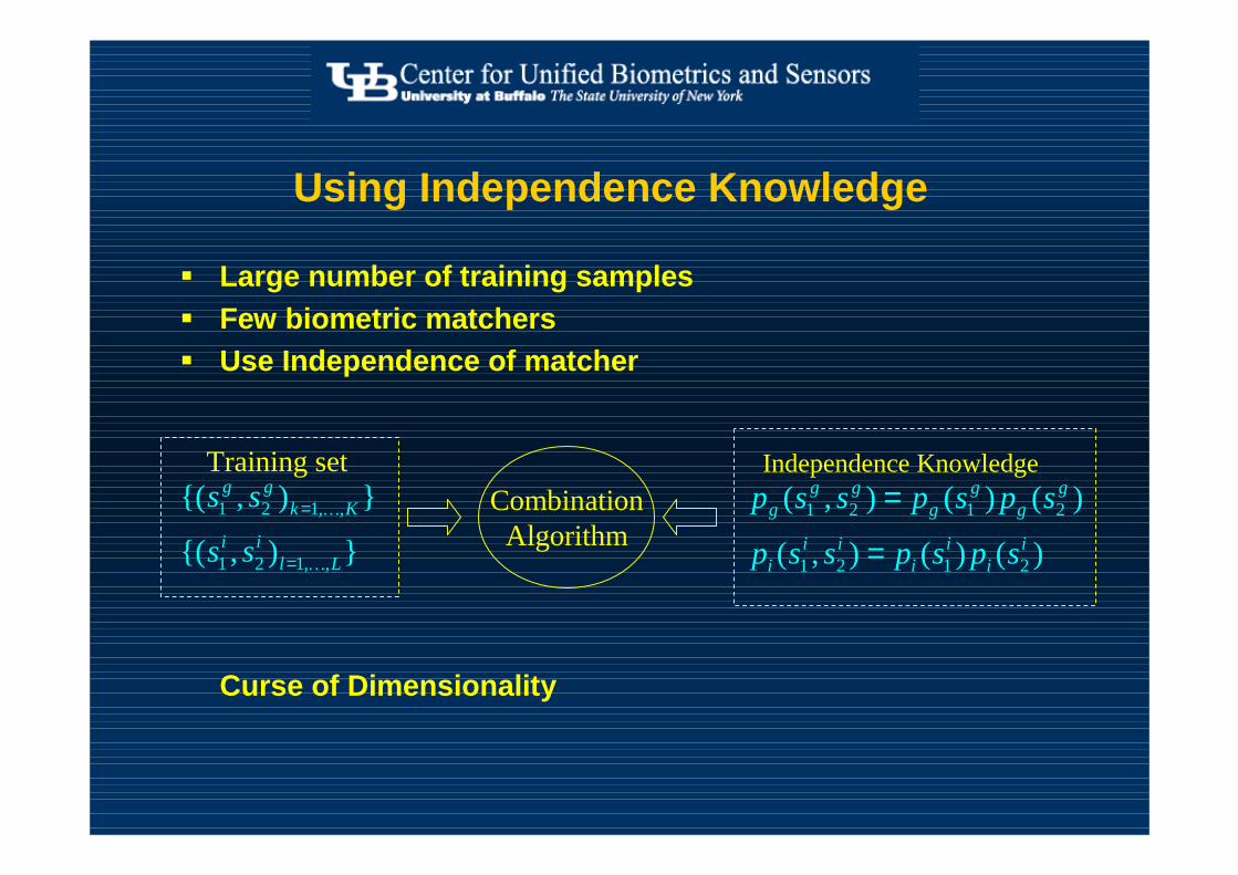
Using Independence Knowledge
� Large number of training samples� Few biometric matchers� Use Independence of matcher
Curse of Dimensionality
}),{(
}),{(
,,121
,,121
Llii
Kkgg
ss
ss
…
…
=
=
Training setCombinationAlgorithm
)()(),(
)()(),(
2121
2121
ii
ii
iii
gg
gg
ggg
spspssp
spspssp
=
=Independence Knowledge

Use Parzen KernelsApproximate densities for Bayesian classification:
• 2-dimensional kernels
• Using independence - approximate 2-dimensional score densities by products of 1-dimensional kernel
∑=
−−=≈N
i h
six
h
six
hNsspssp
1
22112121
)(,
)(11),(ˆ),( ϕ
∑=
−=
≈=N
i h
six
hNsp
spspspspssp
1
111
212121
)(11)(ˆ
)(ˆ)(ˆ)()(),(
ϕ
Subscripts gen and imp have been dropped.
h is estimated using Maximum Likelihood criterion in each case

Estimation ErrorsMean integrated squared error (MISE) is a measure of pdf estimation:
−= ∫
∞
∞−
dxxppEpMISE )()ˆ()ˆ( 2
For d-dimensional kernel estimation of pdf the order of error is:
dk
k
npMISE +−
2
2
~)ˆ(
22
2
12
2
+−
+−
< k
k
k
k
nn
W. Hardle “Smoothing techniques with implementation in S”
Known: lower dimension d results in better asymptotic pdf approximation. In particular, error for approximating 1-dimensional pdf is less than error for approximating 2-dimensional pdf given same no. of training samples
n = no. of training samples
d = no. of dimensions
k= no. of parameters in derivation; consider a constant
Theorem: Product of approximations has the same order of error as individual 1-dimensional approximations. [Tulyakov 06]
For given n (usually small and fixed) training samples; and constant k

Experiments
0 0.002 0.004 0.006 0.008 0.01 0.012 0.014 0.016 0.018 0.020
0.02
0.04
0.06
0.08
0.1
0.12
FRR
FAR
2d pdf recons truction1d pdf recons truction
0 0.005 0.01 0.015 0.02 0.025 0.030
0.05
0.1
0.15
0.2
0.25
FRR
FAR
2d pdf recons truction1d pdf recons truction
• NIST BSSR1 biometric score set• 517 enrollees and 517 user authentication attempts • Leave-one-out testing procedure• Score for test sample (Likelihood Ratio) :
• Can use SVM and other classifiers as well. Not all can produce ROC curve)|,(
)|,(
21
21
impostorssp
genuinessp

Summary of Combinations for Verification Tasks
� Can use trainable combination functions instead of fixed rules if classifier is trainable and sufficient training data available
� Can use the score space as feature space
� Likelihood Ratio function is optimal if the probability density functions (PDFs) can be estimated accurately.
� If the individual matchers are independent (as in biometric modalities), the PDFs can be estimated using this information.
� For the same amount of training data (usually limited), estimating lower dimension PDFs is more accurate.