1

Classical Quantum Mechanics Randell L. Mills

Abstract Despite its successes, quantum mechanics (QM) has remained mysterious to all who have en-countered it. Starting with Bohr and progressing into the present, the departure from intuitive, physical reality has widened. The connection between QM and reality is more than just a “phi-losophical” issue. It reveals that QM is not a correct or complete theory of the physical world and that inescapable internal inconsistencies and incongruities arise when attempts are made to treat it as physical as opposed to a purely mathematical “tool.” Some of these issues are discussed in a review by F. Laloë [Am. J. Phys. 69, 655 (2001)]. In an attempt to provide some physical insight into atomic problems and starting with the same essential physics as Bohr of e– moving in the Coulombic field of the proton and the wave equation as modified by Schrödinger, a classical approach is explored that yields a remarkably accurate model and provides insight into physics on the atomic level. The proverbial view, deeply seated in the wave-particle duality notion, that there is no large-scale physical counterpart to the nature of the electron may not be correct. Physical laws and intuition may be restored when dealing with the wave equation and quantum-mechanical problems. Specifically, a theory of classical quantum mechanics (CQM) is derived from first principles that successfully applies physical laws on all scales. Rather than using the postulated Schrödinger boundary condition “Ψ → 0 as r → ∞,” which leads to a purely mathe-matical model of the electron, the constraint is based on experimental observation. Using Max-well’s equations, the classical wave equation is solved with the constraint that the bound (n = 1)-state electron cannot radiate energy. By further application of Maxwell’s equations to electro-magnetic and gravitational fields at particle production, the Schwarzschild metric is derived from the classical wave equation, which modifies general relativity to include conservation of space-time in addition to momentum and matter/energy. The result gives a natural relationship among Maxwell’s equations, special relativity, and general relativity. CQM holds over a scale of space-time of 85 orders of magnitude — it correctly predicts the nature of the universe from the scale of the quarks to that of the cosmos. A review is given by G. Landvogt [Internat. J. Hydrogen Energy 28, 1155 (2003)].

Key words: Maxwell’s equations, nonradiation, quantum theory, special and general relativity, particle masses, cosmology, wave equation

1. INTRODUCTION

The hydrogen atom is the only real problem for which the Schrödinger equation can be solved without approximations; however, it only provides three quantum numbers, not four, and ines-capable disagreements between observation and predictions arise from the later postulated Dirac equation as well as the Schrödinger equation.(3–5) Furthermore, physical laws, such as Maxwell’s equations, have a physical basis, unlike Dirac’s and Schrödinger’s equations, which must be ac-cepted without any underlying physical basis for fundamental observables such as the stability of the hydrogen atom in the first place, which is always disconcerting to those that study quantum mechanics (QM). In this instance, a circular argument regarding definitions for parameters in the

2

wave equation solutions and the Rydberg series of spectral lines replaces a prediction of those lines based on first principles.(3–5) Nevertheless, the application of the Schrödinger equation to real problems has provided useful approximations for physicists and chemists. Schrödinger in-terpreted eΨ*(x)Ψ(x) as the charge density or the amount of charge between x and x + dx (Ψ* is the complex conjugate of Ψ). Presumably, then, he pictured the electron to be spread over large regions of space. Max Born, who was working with scattering theory, later found that Schrödinger’s interpretation led to inconsistencies, so he replaced it with the probability of find-ing the electron between x and x + dx as *( ) ( ) .x x dxΨ Ψ∫ (1) Born’s interpretation is generally accepted. Nonetheless, interpretation of the wave-function is a never-ending source of confusion and conflict. Many scientists have solved this problem by con-veniently adopting the Schrödinger interpretation for some problems and the Born interpretation for others. This duality allows the electron to be everywhere at one time — yet have no volume. Alternatively, the electron can be viewed as a discrete particle that moves here and there (from r = 0 to r = ∞), and ΨΨ* gives the time average of this motion. Despite its successes, after decades of futility, QM and the intrinsic Heisenberg uncertainty principle have not yielded a unified the-ory, are still purely mathematical, and have yet to be shown to be based on reality.(5) Both are based on circular arguments that the electron is a point with no volume with a vague probability wave requiring that the electron have multiple positions and energies including negative and in-finite energies simultaneously. It may be time to revisit the 75-year-old notion that fundamental particles such as the electron are one- or zero-dimensional and obey different physical laws than objects comprising fundamental particles and the even more disturbing view that fundamental particles don’t obey physical laws — rather they obey mathematics devoid of physical laws. Per-haps mathematics does not determine physics. It only models physics.

The Schrödinger equation was originally postulated in 1926 as having a solution of the one-electron atom. It gives the principal energy levels of the hydrogen atom as eigenvalues of eigen-function solutions of the Laguerre differential equation. But, when the principal quantum number n is much greater than 1, the eigenfunctions become nonsensical since they are sinusoidal over all space; thus they are nonintegrable, cannot be normalized, and are infinite.(6) Despite its wide acceptance, on deeper inspection, the Schrödinger equation solution is plagued with many fail-ings as well as difficulties in terms of a physical interpretation that have caused it to remain con-troversial since its inception. Only the one-electron atom may be solved without approximations, but the equation fails to predict electron spin and leads to models with nonsensical consequences such as negative energy states of the vacuum, infinities, and negative kinetic energy. In addition to many predictions, which simply do not agree with observations, the Schrödinger equation and succeeding extensions predict noncausality, nonlocality, spooky actions at a distance or quantum telepathy, perpetual motion, and many internal inconsistencies where contradicting statements have to be taken true simultaneously.(3–5)

It was reported previously(5) that the behavior of free electrons in superfluid helium has again forced the issue of the meaning of the wave-function. Electrons form bubbles in superfluid he-lium, which reveal that the electron is real and that a physical interpretation of the wave-function is necessary. Furthermore, when irradiated with light of energy of about 0.5 to several electron volts,(7) the electrons carry current at different rates as if they exist with different sizes. It has been proposed that the behavior of free electrons in superfluid helium can be explained in terms of the electron breaking into pieces at superfluid helium temperatures.(7) Yet the electron has proved to be indivisible even under particle accelerator collisions at 90 GeV (Large Electron

3

Positron Collider II). The nature of the wave-function needs to be addressed. It is time for the physical rather than the mathematical nature of the wave-function to be determined.

From the time of its inception, QM has been controversial because its foundations are in con-flict with physical laws and are internally inconsistent. Interpretations of QM such as hidden variables, multiple worlds, consistency rules, and spontaneous collapse have been put forward in an attempt to base the theory in reality. Unfortunately, many theoreticians ignore the requirement that the wave-function be real and physical in order for it to be considered a valid description of reality. For example, regarding this issue, Fuchs and Peres believe,(8) “Contrary to those desires, quantum theory does not describe physical reality. What it does is provide an algorithm for com-puting probabilities for macroscopic events (‘detector ticks’) that are the consequences of our experimental interventions. This strict definition of the scope of quantum theory is the only in-terpretation ever needed, whether by experimenters or theorists.”

With Penning traps, it is possible to measure transitions including those with hyperfine levels of electrons of single ions. This case can be experimentally distinguished from statistics over equivalent transitions in many ions. Whether many or one, the transition energies are always identical within the resonant line width. So probabilities have no place in describing atomic en-ergy levels. Moreover, quantum theory is incompatible with probability theory since it is based on underlying unknown, but determined, outcomes, as discussed previously.(5)

The Copenhagen interpretation provides another meaning of QM. It asserts that what we ob-serve is all we can know; any speculation about what an electron, photon, atom, or other atomic-sized entity is really or what it is doing when we are not looking is just that — speculation. The postulate of quantum measurement asserts that the process of measuring an observable forces it into a state of reality. In other words, reality is irrelevant until a measurement is made. In the case of electrons in superfluid helium, the fallacy with this position is that the “ticks” (migration times of electron bubbles) reveal that the electron is real before a measurement is made. Fur-thermore, experiments on transitions on single ions such as Ba+ in a Penning trap under continu-ous observation demonstrate that the postulate of quantum measurement of QM is experimen-tally disproved, as discussed previously.(5,9) These issues and other such flawed philosophies and interpretations of experiments that arise from QM were discussed previously.(3–5)

QM gives correlations with experimental data. It does not explain the mechanism for the ob-served data. But it should not be surprising that it gives good correlations given that the con-straints of internal consistency and conformance to physical laws are removed for a wave equa-tion with an infinite number of solutions, where the solutions may be formulated as an infinite series of eigenfunctions with variable parameters. There are no physical constraints on the pa-rameters. They may even correspond to unobservables such as virtual particles, hyperdimen-sions, effective nuclear charge, polarization of the vacuum, worm holes, spooky action at a dis-tance, infinities, parallel universes, and faster than light travel. If the constraints of internal con-sistency and conformance to physical laws are invoked, QM has never successfully solved a physical problem.

Throughout the history of quantum theory, wherever there was an advance to a new applica-tion, it was necessary to repeat a trial-and-error experiment to find which method of calculation gave the right answers. Often the textbooks present only the successful procedure as if it fol-lowed from first principles and do not mention the actual method by which it was found. In elec-tromagnetic theory based on Maxwell’s equations, one deduces the computational algorithm from the general principles. In quantum theory, the logic is just the opposite. One chooses the principle to fit the empirically successful algorithm. For example, we know that it required a great deal of art and tact over decades of effort to get correct predictions out of quantum electro-dynamics (QED). For the right experimental numbers to emerge, one must do the calculation (i.e. subtract off the infinities) in one particular way and not in some other way that appears in princi-

4

ple equally valid. There is a corollary, noted by Kallen: from an inconsistent theory, any result may be derived.

Reanalysis of old experiments and many new experiments including electrons in superfluid he-lium challenge the Schrödinger equation predictions. Many noted physicists have rejected QM. Feynman also attempted to use first principles including Maxwell’s equations to discover new physics to replace QM.(10) Other great physicists of the 20th century have searched: “Einstein … insisted … that a more detailed, wholly deterministic theory must underlie the vagaries of quan-tum mechanics.”(11) He felt that scientists were misinterpreting the data. These issues and the results of many experiments, such as the wave-particle duality, the Lamb shift, anomalous mag-netic moment of the electron, transition and decay lifetimes, and experiments invoking interpre-tations of spooky action at a distance such as the Aspect experiment, entanglement, and double-slit-type experiments, are shown to be absolutely predictable and physical in the context of a theory of classical quantum mechanics (CQM) derived from first principles.(3–5) Using the classi-cal wave equation with the constraint of nonradiation based on Maxwell’s equations, CQM gives closed-form physical solutions for the electron in atoms, the free electron, and the free electron in superfluid helium, which match the observations without requiring that the electron be divisi-ble. Moreover, unification of atomic and large-scale physics — the ultimate objective of natural theory — is enabled. CQM holds over a scale of space-time of 85 orders of magnitude — it cor-rectly predicts the nature of the universe from the scale of the quarks to that of the cosmos.

2. CLASSICAL QUANTUM THEORY OF THE ATOM BASED ON MAXWELL’S EQUATIONS THAT HOLDS OVER ALL SCALES

In this paper the old view that the electron is a zero- or one-dimensional point in an all-space probability wave-function Ψ(x) is not taken for granted. The theory of CQM, derived from first principles, must successfully and consistently apply physical laws on all scales.(3–5) Historically, the point at which QM broke with classical laws can be traced to the issue of nonradiation of the one-electron atom that was addressed by Bohr with a postulate of stable orbits in defiance of the physics represented by Maxwell’s equations.(3−5) Later, physics was replaced by “pure mathemat-ics” based on the notion of the inexplicable wave-particle duality nature of electrons, which lead to the Schrödinger equation, where the consequences of radiation predicted by Maxwell’s equa-tions were ignored. Ironically, both Bohr and Schrödinger used the electrostatic Coulomb poten-tial of Maxwell’s equations but abandoned the electrodynamic laws. Physical laws may indeed be the root of the observations thought to be “purely quantum mechanical,” and it may have been a mistake to make the assumption that Maxwell’s electrodynamic equations must be rejected at the atomic level. Thus, in the present approach, the classical wave equation is solved with the constraint that a bound (n = 1)-state electron cannot radiate energy.

Thus, here, derivations consider the electrodynamic effects of moving charges as well as the Coulomb potential, and the search is for a solution representative of the electron where there is acceleration of charge motion without radiation. The mathematical formulation for zero radiation based on Maxwell’s equations follows from a derivation by Haus.(12) The function that describes the motion of the electron must not possess space-time Fourier components that are synchronous with waves traveling at the speed of light. Similarly, nonradiation is demonstrated based on the electron’s electromagnetic fields and the Poynting power vector.

In this paper a summary of the results of CQM(3,13,14) is presented. (The details of the deriva-tions are given in Ref. 3.) Specifically, CQM gives closed-form solutions for the atom including the stability of the n = 1 state and the instability of the excited states, the equation of the photon and electron in excited states, and the equation of the free electron and photon, which predict the wave-particle duality behavior of particles and light. The current and charge density functions of the electron may be directly physically interpreted. For example, spin angular momentum results

5

from the motion of negatively charged mass moving systematically, and the equation for angular momentum, r × p, can be applied directly to the wave-function (a current density function) that describes the electron. The magnetic moment of a Bohr magneton, Stern–Gerlach experiment, g factor, Lamb shift, resonant line width and shape, selection rules, correspondence principle, wave-particle duality, excited states, reduced mass, rotational energies, momenta, orbital and spin splitting, spin-orbital coupling (fine structure), Knight shift, spin-nuclear coupling (hyper-fine structure), muonium hyperfine structure interval, ionization energies of multi-electron at-oms, elastic electron scattering from helium atoms, and nature of the chemical bond are derived in closed-form equations based on Maxwell’s equations. The calculations agree with experimen-tal observations.

For any kind of wave advancing with limiting velocity and capable of transmitting signals, the equation of front propagation is the same as the equation for the front of a light wave. By apply-ing this condition to electromagnetic and gravitational fields at particle production, the Schwarzschild metric (SM) is derived from the classical wave equation, which modifies general relativity to include conservation of space-time as a consequence of (175) (See Ref. 3, Chap. 23, and footnote 7 of Chap. 23), in addition to momentum and matter/energy. The result gives a natural relationship between Maxwell’s equations, special relativity, and general relativity. It gives gravitation from the atom to the cosmos. The universe is time harmonically oscillatory in matter energy and space-time expansion and contraction with a minimum radius that is the gravi-tational radius. In closed-form equations with fundamental constants only, CQM gives the de-flection of light by stars, the precession of the perihelion of Mercury, the particle masses, the Hubble constant, the age of the universe, the observed acceleration of the expansion, the power of the universe, the power spectrum of the universe, the microwave background temperature, the uniformity of the microwave background radiation at 2.7 K with the microkelvin spatial variation observed by the degree angular scale interferometer (DASI), the observed violation of the GZK cutoff, the mass density, the large-scale structure of the universe, and the identity of dark matter, which matches the criteria for the structure of galaxies. In a special case where the gravitational potential energy density of a black hole equals that of the Planck mass, matter converts to energy and space-time expands with the release of a gamma-ray burst. The singularity in the SM is eliminated.

3. ONE-ELECTRON ATOMS One-electron atoms include the hydrogen atom, He+, Li2+, Be3+, and so on. The mass energy

and angular momentum of the electron are constant; this requires that the equation of motion of the electron be temporally and spatially harmonic. Thus the classical wave equation applies and

2

22 2

1 ( , , , ) 0,r tv t

ρ θ φ⎛ ⎞∂∇ − =⎜ ⎟∂⎝ ⎠

(2)

where ρ(r, θ, φ, t) is the time-dependent charge density function of the electron in time and space. In general, the wave equation has an infinite number of solutions. To arrive at the solution that represents the electron a suitable boundary condition must be imposed. It is well known from experiments that each single atomic electron of a given isotope radiates to the same stable state. Thus the physical boundary condition of nonradiation of the bound electron was imposed on the solution of the wave equation for the time-dependent charge density function of the elec-tron.(3) The condition for radiation by a moving point charge given by Haus(12) is that its space-time Fourier transform possess components that are synchronous with waves traveling at the

6

speed of light. Conversely, it is proposed that the condition for nonradiation by an ensemble of moving point charges that makes up a current density function is as follows:

For nonradiative states, the current density function must not possess space-time Fourier components that are synchronous with waves traveling at the speed of light.

The time, radial, and angular solutions of the wave equation are separable. The motion is time harmonic with frequency ωn. A constant angular function is a solution to the wave equation. So-lutions of the Schrödinger wave equation making up a radial function radiate according to Max-well’s equation, as shown previously by application of Haus’s condition.(3) In fact, it was found that any function that permitted radial motion gave rise to radiation. A radial function that satis-fies the boundary condition is a radial delta function

2

1( ) ( ).nf r r rr

δ= − (3)

This function defines a constant charge density on a spherical shell where rn = nr1, where n is an integer in an excited state as given in Section 13, and (2) becomes the two-dimensional wave equation plus time with separable time and angular functions. Given time harmonic motion and a radial delta function, the relationship between an allowed radius and the electron wavelength is given by 2 ,n nrπ λ= (4) where the subscript n is determined during photon absorption as given by (77). Using the ob-served de Broglie relationship for the electron mass, where the coordinates are spherical (this relationship is derived in Chap. 3 of Ref. 3), we have

,nn e n

h hp m v

λ = = (5)

and the magnitude of the velocity for every point on the orbitsphere is

.ne n

vm r

= (6)

The sum of |Li|, the magnitude of the angular momentum of each infinitesimal point of the or-bitsphere of mass mi, must be constant. The constant is :

.i i e ne n

m m rm r

Σ | |= Σ | × |= =L r v (7)

Thus an electron is a spinning, two-dimensional spherical surface (zero thickness1), called an electron orbitsphere, that can exist in a bound state at only specified distances from the nucleus, as shown in Fig. 1. The corresponding current function shown in Fig. 2, which gives rise to the

7

phenomenon of spin, is derived in Section 4. (See the Appendix of this paper and the Orbitsphere Equation of Motion for = 0 section of Ref. 3 at Chap. 1.)

Nonconstant functions are also solutions for the angular functions. To be a harmonic solution of the wave equation in spherical coordinates, these angular functions must be spherical har-monic functions.(15) A zero of the space-time Fourier transform of the product function of two spherical harmonic angular functions, a time harmonic function, and an unknown radial function is sought. The solution for the radial function that satisfies the boundary condition is also a delta function given by (3). Thus bound electrons are described by a charge density (mass density) function that is the product of a radial delta function, two angular functions (spherical harmonic functions), and a time harmonic function:

2

1( , , , ) ( ) ( , , ) ( ) ( , , ); ( , , ) ( , ) ( ).nr t f r A t r r A t A t Y k tr

ρ θ φ θ φ δ θ φ θ φ θ φ= = − = (8)

In these cases the spherical harmonic functions correspond to a traveling charge density wave confined to the spherical shell, which gives rise to the phenomenon of orbital angular momen-tum. The orbital functions that modulate the constant “spin” function shown graphically in Fig. 3 are given in Section 5.

4. SPIN FUNCTION The orbitsphere spin function comprises a constant charge (current) density function with mov-

ing charge confined to a two-dimensional spherical shell. The current pattern of the orbitsphere spin function comprises an infinite series of correlated orthogonal great circle current loops where each point charge (current) density element moves time harmonically with constant angu-lar velocity

2 .ne nm r

ω = (9)

The uniform current density function Y0

0(θ , φ), the orbitsphere equation of motion of the electron (14)–15), corresponding to the constant charge function of the orbitsphere that gives rise to the spin of the electron, is generated from a basis set current vector field defined as the orbitsphere current vector field (orbitsphere-cvf). This in turn is generated over the surface by two comple-mentary steps of an infinite series of nested rotations of two orthogonal great circle current loops, where the coordinate axes rotate with the two orthogonal great circles that serve as a basis set. The algorithm to generate the current density function rotates the great circles and the corre-sponding x′y′z′ coordinates relative to the xyz frame. Each infinitesimal rotation of the infinite series is about the new i′ axis and new j′ axis resulting from the preceding such rotation. Each element of the current density function is obtained with each conjugate set of rotations. In Ap-pendix III of Ref. 3, the continuous uniform electron current density function Y0

0(θ, φ) ((14) and (15)) is then exactly generated from this orbitsphere-cvf as a basis element by a convolution op-erator comprising an autocorrelation-type function.

For Step 1, the current density elements move counterclockwise on the great circle in the y′z′ plane and clockwise on the great circle in the x′z′ plane. The great circles are rotated by an infini-tesimal angle ±∆αi′ (a positive rotation around the x′ axis and a negative rotation about the z′ axis for Steps 1 and 2, respectively) and then by ±∆αj′ (a positive rotation around the new y′ axis and a positive rotation about the new x′ axis for Steps 1 and 2, respectively). The coordinates of each point on each rotated great circle (x′, y′, z′) are expressed in terms of the first (x, y, z) coordinates

8

by the following transforms, where clockwise rotations and motions are defined as positive look-ing along the corresponding axis. Note the abbreviations of c for cosine and s for sine to save space. Step 1:

c( ) 0 s( ) 1 0 00 1 0 0 c( ) s( )

s( ) 0 c( ) 0 s( ) c( )

c( ) s( )s( ) s( ) c( )0 c( ) s( )

s( ) c( )s( ) c( ) c( )

y y

x x

y y x x

y y x y x

x x

y y x y x

x xy yz z

x

α αα α

α α α α

α α α α αα α

α α α α α

′⎡ ⎤∆ − ∆⎡ ⎤ ⎡ ⎤ ⎡ ⎤⎢ ⎥⎢ ⎥ ⎢ ⎥ ⎢ ⎥′= × ∆ ∆⎢ ⎥⎢ ⎥ ⎢ ⎥ ⎢ ⎥⎢ ⎥ ′⎢ ⎥ ⎢ ⎥ ⎢ ⎥∆ ∆ − ∆ ∆⎣ ⎦ ⎣ ⎦ ⎣ ⎦⎣ ⎦

′⎡ ⎤∆ ∆ ∆ − ∆ ∆⎢ ⎥ ′= ∆ ∆⎢ ⎥⎢ ⎥∆ − ∆ ∆ ∆ ∆⎣ ⎦

.yz

⎡ ⎤⎢ ⎥⎢ ⎥

′⎢ ⎥⎣ ⎦

(10)

Step 2:

1 0 0 c( ) s ( ) 00 c( ) s( ) s ( ) c( ) 00 s( ) c( ) 0 0 1

c( ) s ( ) 0c( )s ( ) c( )c( ) s( )

s( )s ( ) s( )c( ) c( )

z z

x x z z

x x

z z

x z x z x

x z x z x

x xy yz z

xy

α αα α α αα α

α αα α α α α

α α α α α

′∆ ∆⎡ ⎤ ⎡ ⎤ ⎡ ⎤ ⎡ ⎤⎢ ⎥ ⎢ ⎥ ⎢ ⎥ ⎢ ⎥′= ∆ ∆ − ∆ ∆⎢ ⎥ ⎢ ⎥ ⎢ ⎥ ⎢ ⎥

′⎢ ⎥ ⎢ ⎥ ⎢ ⎥ ⎢ ⎥− ∆ ∆⎣ ⎦ ⎣ ⎦ ⎣ ⎦ ⎣ ⎦′∆ ∆⎡ ⎤

⎢ ⎥ ′= − ∆ ∆ ∆ ∆ ∆⎢ ⎥⎢ ⎥∆ ∆ − ∆ ∆ ∆⎣ ⎦

.z

⎡ ⎤⎢ ⎥⎢ ⎥

′⎢ ⎥⎣ ⎦

(11)

The angular sum in (10) and (11) is

,

22

,0 1

2 .lim 2

i j

i jn

π

α

αα π

′ ′|∆ |

′ ′∆ → =

| ∆ | =∑

The orbitsphere-cvf is given by n reiterations of (10) and (11) for each point on each of the two

orthogonal great circles during each of Steps 1 and 2. The output given by the nonprimed coor-dinates is the input of the next iteration corresponding to each successive nested rotation by the infinitesimal angle ±∆αi′ or ±∆αj′, where the magnitude of the angular sum of the n rotations about the i′ axis and the j′ axis is ( 2 /2)π. Half of the orbitsphere-cvf is generated during each of Steps 1 and 2.

Following Step 2, in order to match the boundary condition that the magnitude of the velocity at any given point on the surface is given by (6), the output half of the orbitsphere-cvf is rotated clockwise by an angle of π /4 about the z axis. Using (11) with ∆αz′ = π/4 and ∆αx′ = 0 gives the rotation. Then the one half of the orbitsphere-cvf generated from Step 1 is superimposed with the complementary half obtained from Step 2 following its rotation about the z axis of π /4 to give the basis function to generate Y0

0(θ , φ), the orbitsphere equation of motion of the electron, by convolution about the resultant angular momentum axis.

9

The current pattern of the orbitsphere-cvf generated by the nested rotations of the orthogonal great circle current loops is a continuous and total coverage of the spherical surface, but it is shown as a visual representation using 6° increments of the infinitesimal angular variable ±∆αi′ or ±∆αj′ of (10) and (11) from the perspective of the z axis in Fig. 2. In each case, the complete orbitsphere current pattern corresponds to all the orthogonal great circle elements generated by the rotation of the basis set according to (10) and (11), where ±∆αi′ and ±∆αj′ approach zero and the summation of the infinitesimal angular rotations of ±∆αi′ and ±∆αj′ about the successive i′ axes and j′ axes is ( 2 /2)π for each step.

The resultant angular momentum projections of Lxy = /4 and Lz = /2 meet the boundary con-dition for the unique current with angular velocity magnitude at each point on the surface given by (6) and give rise to the Stern–Gerlach experiment, as shown in Ref. 3. The further constraint that the current density is uniform such that the charge density is uniform, corresponding to an equipotential, minimum energy surface, is satisfied by using the orbitsphere-cvf as a basis ele-ment to generate Y0

0(θ, φ) using a convolution operator comprising an autocorrelation-type func-tion, as given in Appendix III of Ref. 3. The operator comprises the convolution of each great circle current loop of the orbitsphere-cvf designated as the primary orbitsphere-cvf with a second orbitsphere-cvf designated as the secondary orbitsphere-cvf having its angular momentum matched to that of each convoluted current loops such that the resulting exact uniform current distribution obtained from the convolution has the same components of Lxy = /4 and Lz = /2 as those of the orbitsphere-cvf used as a primary basis element. The current pattern gives rise to the phenomenon corresponding to the spin quantum number. The details of the derivation of the spin function are given in the Appendix of this paper and in Chapter 1 of Ref. 3.

5. ANGULAR FUNCTIONS The time, radial, and angular solutions of the wave equation are separable. Also, based on the

radial solution, the angular charge and current density functions of the electron, A(θ, φ, t), must be a solution of the wave equation in two dimensions (plus time):

2

22 2

1 ( , , ) 0,A tv t

θ φ⎡ ⎤∂∇ − =⎢ ⎥∂⎣ ⎦

(12)

where ρ(r, θ, φ, t) = f(r)A(θ, φ, t) = (1/r2)δ(r – rn)A(θ, φ, t) and A(θ, φ, t) = Y(θ, φ)k(t):

( )2 2

2 2 2 2 2 2, ,

1 1 1sin , , 0,sin sinr r

A tr r v tφ θ

∂θ θ φθ θ θ θ φ ∂

⎡ ⎛ ⎞ ⎤∂ ∂ ∂⎛ ⎞ + − =⎢ ⎜ ⎟⎜ ⎟ ⎥∂ ∂ ∂⎝ ⎠⎢ ⎝ ⎠ ⎦⎣ (13)

where v is the linear velocity of the electron. The charge density functions including the time function factor are

002( , , , ) [ ( )][ ( , ) ( , )]

8m

ner t r r Y Yr

ρ θ φ δ θ φ θ φπ

= − + (14)

for = 0 and

10

002( , , , ) [ ( )][ ( , ) Re ( , ) ]

4ni tm

ner t r r Y Y er

ωρ θ φ δ θ φ θ φπ

= − + (15)

for ≠ 0, where Y m(θ, φ) are the spherical harmonic functions that spin about the z axis with angular frequency ωn with Y0

0(θ, φ) the constant function. ReY m(θ, φ) ni te ω = P m(cos θ)cos (mφ + ωn′t), where, to keep the form of the spherical harmonic as a traveling wave about the z axis, ωn′ = mωn.

6. ACCELERATION WITHOUT RADIATION 6.1 Special Relativistic Correction to the Electron Radius

The relationship between the electron wavelength and its radius is given by (4), where λ is the de Broglie wavelength. For each current density element of the spin function, the distance along each great circle in the direction of instantaneous motion undergoes length contraction and time dilation. Using a phase-matching condition, the wavelengths of the electron and laboratory iner-tial frames are equated, and the corrected radius is given by

3/ 2 3/ 22 2 211 sin 1 cos 1 ,2 2 2n n

v v vr rc c c

π ππ

⎡ ⎤⎡ ⎤ ⎡ ⎤⎛ ⎞ ⎛ ⎞⎛ ⎞ ⎛ ⎞ ⎛ ⎞⎢ ⎥⎢ ⎥ ⎢ ⎥′= − − + −⎜ ⎟ ⎜ ⎟⎜ ⎟ ⎜ ⎟ ⎜ ⎟⎜ ⎟ ⎜ ⎟⎢ ⎥⎢ ⎥ ⎢ ⎥⎝ ⎠ ⎝ ⎠ ⎝ ⎠⎝ ⎠ ⎝ ⎠⎣ ⎦ ⎣ ⎦⎣ ⎦

(16)

where the electron velocity is given by (6) (see Ref. 3, Chap. 1, Special Relativistic Correction to the Ionization Energies section). e/me of the electron, the electron angular momentum of , and µB are invariant, but the mass and charge densities increase in the laboratory frame due to the relativistically contracted electron radius. As v → c, r/r′ → 1/2π and r = λ, as shown in Fig. 4. 6.2 Nonradiation Based on Haus’s Condition The Fourier transform of the electron charge density function given by (8) is a solution of the

three-dimensional wave equation in frequency space (k, ω space), as given in Chapter 1, Space-Time Fourier Transform of the Electron Function section, of Ref. 3. Then the corresponding Fourier transform of the current density function K(s, Θ, Φ, ω) is given by multiplying by the constant angular frequency:

( )( )

( )( )

2( 1)12

21

2( 1)12

21

( 1) sinsin(2 ) (1/ 2) ( 1/ 2) 2 !( , , ) 4 22 ( 1)!( 1)! ( 1)!cos 2

( 1) sin (1/ 2) ( 1/ 2) 2 !2( 1)!( 1)! ( 1)!cos 2

n nn

n n

s rK s ss r

s

υυυ

υ υυ

υυυ

υ υυ

π υ υω πω πυ υ υπ

π υ υπυ υ υπ

−−∞−

+1 +1=

−−∞−

+1 +1=

⎡ ⎤− Θ Γ Γ +Θ,Φ = ⊗ ⎢ ⎥

− − −Θ⎢ ⎥⎣ ⎦⎡ − Φ ⎤Γ Γ +

⊗ ⎢− − −Φ ⎦⎢⎣

∑

∑ 1 [ ( ) ( )].4 n nδ ω ω δ ω ωπ

− + +⎥

(17)

sn ⋅ vn = sn ⋅ c = ωn implies rn = λn, which is given by (16) in the case that k is the light-like k0. In this case, (17) vanishes. Consequently, space-time harmonics of ωn/c = k or (ωn/c) 0/ε ε = k for which the Fourier transform of the current density function is nonzero do not exist. Radiation due to charge motion does not occur in any medium when this boundary condition is met. (Non-radiation is also determined from the fields based on Maxwell’s equations as given in Section 6.3 below and the same section of Chapter 1, Appendix I, of Ref. 3.) 6.3 Nonradiation Based on the Electron Electromagnetic Fields and the Poynting Power

Vector

11

A point charge undergoing periodic motion accelerates and as a consequence radiates accord-ing to the Larmor formula

2

23

0

1 2 ,4 3

eP acπε

= (18)

where e is the charge, a is its acceleration, ε0 is the permittivity of free space, and c is the speed of light. Although an accelerated point particle radiates, an extended distribution modeled as a superposition of accelerating charges does not have to radiate.(12,16–19) An ensemble of charges, all oscillating at the same frequency, create a radiation pattern with a number of nodes. The same applies to current patterns in phased array antenna design.(20) It is possible to have an infinite number of charges oscillating in such as way as to cause destructive interference or nodes in all directions. The electromagnetic far field is determined from the current distribution in order to obtain the condition, if it exists, that the electron current distribution given by (21) must satisfy so that the electron does not radiate.

The charge density functions of the electron orbitsphere in spherical coordinates plus time are given by (14) and (15). For = 0, the equipotential, uniform, or constant charge density function (14) further comprises a current pattern given in Section 4. It also corresponds to the nonradia-tive n = 1, = 0 state of atomic hydrogen and to the spin function of the electron. The current density function is given by multiplying (14) by the constant angular velocity ω. There is accel-eration without radiation. In this case, it is centripetal acceleration. A static charge distribution exists even though each point on the surface is accelerating along a great circle. Haus’s condition predicts no radiation for the entire ensemble. The same result is trivially predicted from consid-eration of the fields and the radiated power. Since the current is not time dependent, the fields are given by ∇× =H J (19) and 0,∇× =E (20) which are the electrostatic and magnetostatic cases, respectively, with no radiation.

The nonradiation condition given by (17) may be confirmed by determining the fields and the current distribution condition that is nonradiative based on Maxwell’s equations. For ≠ 0, the charge density functions including the time function factor are given by (15). In the cases that m ≠ 0, (15) is a traveling charge density wave that moves on the surface of the orbitsphere about the z axis and modulates the orbitsphere corresponding to = 0. Since the charge is moving time harmonically about the z axis with frequency ωn and the current density function is given by the time derivative of the charge density function, the current density function is given by the nor-malized product of the constant angular velocity and the charge density function. The first cur-rent term of (15) is static. Thus it is trivially nonradiative.

The current due to the time-dependent term is

12

ˆ,

[ ( )]Re ( , )[ ( ) ]

[ ( )]Re ( , ) [ ]

[ ( )]Re( (cos ) )[ ]

[ ( )]( (cos )cos( ))[ ]

[ ( )]( (cos )cos( ))sin

n

n

mn

i tmn

i tm imn

mn n

mn n

N r r Y t

N r r Y e

N r r P e e

N r r P m t

N r r P m t

ω

ωφ

φ

δ θ φ

δ θ φ

δ θ

δ θ φ ω

δ θ φ ω θ

′

= − ×

= − ×

′= − ×

′ ′= − + ×

′ ′= − +

J u r

u r

u r

u r

AAAAA

(21)

where we have used the abbreviation

22 4n

n

er

ωπ π

=A

to save space, and, to keep the form of the spherical harmonic as a traveling wave about the z axis, ωn′ = mωn and N and N′ are normalization constants. The vectors are defined as

ˆ ˆ ˆ ˆˆ ,ˆ ˆ| | sin

ˆ ˆ orbital axis,

u r u ru r

u z

φθ

× ×= =

×= =

(22)

ˆ ˆ ˆ,rθ φ= × (23) where ^ denotes unit vectors (e.g., u = u/|u|), nonunit vectors are designated in bold, and the current function is normalized. For time-varying electromagnetic fields, Jackson(21) gives a gen-eralized expansion in vector spherical waves, which are convenient for electromagnetic boundary value problems possessing spherical symmetry properties and for analyzing multipole radiation from a localized source distribution. The Green function G(x′, x) that is appropriate to the equa-tion 2 2( ) ( , ) ( )k G δ′ ′∇ + = − −x x x x (24) in the infinite domain is

(1) *, ,

0( , ) ( ) ( ) ( , ) ( , ).

ik

m mm

eG ik j kr h kr Y Yθ φ θ φ′− | − | ∞

< >= =−

′ ′ ′= =′| − | ∑ ∑

x x

x xx x

(25)

where the spherical wave expansion for the outgoing wave is given. General coordinates are shown in Fig. 5. Jackson(21) further gives the general multipole field solution to Maxwell’s equa-tions in a source-free region of empty space with the assumption of a time dependence eiωnt :

, ,,

, ,,

( , ) ( ) ( , ) ( ) ,

( , ) ( ) ( , ) ( ) ,

E m M mm

E m M mm

ia m f kr a m g krk

i a m f kr a m g krk

⎡ ⎤= − ∇×⎢ ⎥⎦⎣

⎡ ⎤= ∇× +⎢ ⎥⎦⎣

∑

∑

B X X

E X X (26)

13

where the cgs units used by Jackson are retained in this section. The radial functions f (kr) and g (kr) are of the form (1) (1) (2) (2)( ) .g kr A h A h= + (27) X ,m is the vector spherical harmonic defined by

, ,1( , ) ( , ),

( 1)m mYθ φ θ φ=+

X L (28)

where

1 ( ).i

= ×∇L r (29)

The coefficients aE( , m) and aM( , m) of (26) specify the amounts of electric ( , m) multipole

and magnetic ( , m) multipole fields and are determined by sources and boundary conditions, as are the relative proportions in (27). Jackson gives the result of the electric and magnetic coeffi-cients from the sources as

*234( , ) [ ( )] ( ) ( ) ( ) ( )

( 1)m

Ek ika m Y rj kr j kr ik j kr d x

r ciπ δρ

δ⎧ ⎫= + ⋅ − ∇ ⋅ ×⎨ ⎬⎩+ ⎭∫ r J r M (30)

and

*2

34( , ) ( ) ,( 1)

mM

ka m j kr Y d xc

π ⎛ ⎞−= ⋅ + ∇×⎜ ⎟

⎝ ⎠+ ∫JL M (31)

respectively, where the distribution of charge ρ(x, t), current J(x, t), and intrinsic magnetization M(x, t) are harmonically varying sources: ρ(x) nte ω− , J(x) nte ω− , and M(x) nte ω− . From (21) the charge and intrinsic magnetization terms are zero. Also, the current J(x, t) is in the φ direction; thus the aE( , m) coefficient given by (30) is zero since r ⋅ J = 0. Substitution of (21) into (31) gives the magnetic multipole coefficient aM( , m):

*22

3

ˆ( ) ( , )sin2 44( , ) ( ) .

( 1)

mnn

m nM

e N r r Yrka m j kr Y d x

c

ω δ θ φ θφπ ππ

⎛ ⎞−⎜ ⎟− ⎜ ⎟= ⋅⎝ ⎠+ ∫ L (32)

Each mass density element of the electron moves about the z axis along a circular orbit of radius rn sin θ in such a way that φ changes at a constant rate. That is, φ = ωt at time t, where ωn is the constant angular frequency given in (21) and ( ) sin cos sin sinn nr t r t r tθ ω θ ω= +i j (33)

14

is the parametric equation of the circular orbit. Jackson gives the operator in the xy plane corre-sponding to the current motion in this plane and the relations for Y m(θ, φ):(21)

cot ,ix yL L iL e iφ ∂ ∂θ

∂θ ∂φ+

⎛ ⎞= + = +⎜ ⎟

⎝ ⎠ (34)

1( , ) ( )( 1) ( , ).m mL Y m m Yθ φ θ φ+

+ = − + + (35)

Using (34), L ⋅ J of (31) is

( ( , ) sin ) cot ( , ) sin

( , ) cot sin sin cot ( , ).

m i m

i m i m

L Y e i Y

e Y i e i Y

φ

φ φ

θ φ θ θ θ φ θθ φ

θ φ θ θ θ θ θ φθ φ θ φ

+

⎛ ⎞∂ ∂= +⎜ ⎟∂ ∂⎝ ⎠

⎛ ⎞ ⎛ ⎞∂ ∂ ∂ ∂= + + +⎜ ⎟ ⎜ ⎟∂ ∂ ∂ ∂⎝ ⎠ ⎝ ⎠

(36)

Using (35) in (36) gives

1( ( , ) sin ) ( , ) cos sin ( )( 1) ( , ).m i m mL Y e Y m m Yφθ φ θ θ φ θ θ θ φ++ = + − + + (37)

The spherical harmonic is given as

,2 1 ( )!( , ) (cos ) (cos ) .4 ( )!

m m im m imm

mY P e N P em

φ φθ φ θ θπ+ −

= =+

(38)

Thus (37) is given as

,

1 ( 1), 1

( ( , ) sin ) (cos ) cos

sin ( )( 1) (cos ) .

m i m imm

m i mm

L Y e N P e

m m N P e

φ φ

φ

θ φ θ θ θ

θ θ+

+ ++

=

+ − + + (39)

Substitution of (39) into (32) gives

( )( )

( ) ( )( )

( )( ) ( ) ( )

2

2

,* 311

, 1

,21

cos cos , ( ) .

sin 1 cos

nM

n

i m immm

n i mmm

k ea m Nrc

e N P ej kr Y r r d x

m m N P e

φ φ

φ

ωπ

θ θθ φ δ

θ θ +++

−=

+

⎧ ⎫⎪ ⎪− ⎨ ⎬+ − + +⎪ ⎪⎩ ⎭

∫ (40)

Substitution of Y –m(θ, φ) = (–1)m(θ, φ) and (38) into (40) and integration with respect to dr gives

15

2

2

,0 0

,

1 ( 1), 1

( , ) ( )2( 1)

( 1) (cos )

[ (cos ) cos

sin ( )( 1)

(cos ) ]sin .

nM n

m m imm

i m imm

m i mm

eka m Nj krc

N P e

e N P e

m m

N P e d d

π πφ

φ φ

φ

ωπ

θ

θ θ

θ

θ θ θ φ

− −−

+ ++

−=

+

−

×

+ − + +

×

∫ ∫ (41)

The integral in (41) separated in terms of dθ and dφ is

( )( )

( )

( ) ( )( )

( )( ) ( ) ( )

2

2,

, 110 0 , 1

,21

cos cos 1 cos sin .

sin 1 cos

nM n

i m immm m im

m i mmm

eka m Nj krc

e N P eN P e d d

m m N P e

φ φπ πφ

φ

ωπ

θ θθ θ θ φ

θ θ− −

− +++

−=

+

⎧ ⎫⎪ ⎪− ⎨ ⎬+ − + +⎪ ⎪⎩ ⎭

∫ ∫ (42) Consider that the dθ integral is finite and designated by Θ. Then (42) is given as

22

0

( , ) ( ) .2( 1)

inM n

eka m Nj kr e dc

πφω φ

π−

= Θ+ ∫ (43)

From (26), the far fields are given by

,

,

( , ) ( ) ,

( , ) ( ) ,

M m

M m

i a m g krk

a m g kr

= − ∇×

=

B X

E X (44)

where aM( , m) is given by (43).

The power density P(t) given by the Poynting power vector is ( ) .P t = ×E H (45) For a pure multipole of order ( , m), the time-averaged power radiated per solid angle dP( , m)/dΩ given by Jackson(21) is

2 2,2

( , ) ( , ) ,8 M m

dP m c a md kπ

= | | | |Ω

X (46)

where aM( , m) is given by (43).

16

Since the modulation function Y ,m(θ, φ) is a traveling charge density wave that moves time harmonically on the surface of the orbitsphere about the z axis with frequency ωn, φ of the spherical harmonic function is a function of t, as shown in (33). The time dependence of the source current must also be evaluated in (43), and it can be written as

2

0

( , )

( ) cos( ( )) ,2( 1)

n

MvT

nn

a m

ek Nj kr mks t dsc

ωπ

−= Θ

+ ∫ (47)

where s′(t) is the angular displacement of the rotating modulation function during one period Tn and v is the linear velocity in the φ direction. Thus

2 2

( , ) ( ) sin( ) ( ) sin( ).2 2( 1) ( 1)

n nM n n n

ek eka m Nj kr mkvT Nj kr mksc c

ω ωπ π

− −= Θ = Θ

+ + (48)

In the case that k is the light-like k0, then k = ωn/c, and the sin (mks) term in (48) vanishes for

1

,

,.

n

n

R cT

RT cRf c

−

=

==

(49)

Thus ,n n ns vT R r λ= = = = (50) as given by (16), which is identical to the Haus condition for nonradiation given by (17). Then the multipole coefficient aM( , m) is zero. For the condition given by (50), the time-averaged power radiated per solid angle dP( , m)/dΩ given by (46) and (48) is zero. There is no radiation.

7. MAGNETIC FIELD EQUATIONS OF THE ELECTRON The orbitsphere is a shell of negative charge current comprising correlated charge motion

along great circles. For = 0, the orbitsphere gives rise to a magnetic moment of one Bohr mag-neton:(22)

24 19.274 10 J T .2B

e

em

µ − −= = × ⋅ (51)

(The details of the derivation of the magnetic parameters including the electron g factor are given in the Appendix of this paper.) The magnetic field of the electron shown in Fig. 6 is given by

17

3

3

( cos sin ) for ,

( 2cos sin ) for .2

r ne n

r ne

e r rm r

e r rm r

θ

θ

θ θ

θ θ

⎧ − <⎪⎪= ⎨⎪ + >⎪⎩

i iH

i i (52)

The energy stored in the magnetic field of the electron is

2

2 20

0 0 0

1 sin ,2magE H r drd d

π π

µ θ θ∞

= Φ∫ ∫ ∫ (53)

2 2

0, 2 3

1

.mag totale

eEm r

πµ= (54)

8. STERN–GERLACH EXPERIMENT The Stern–Gerlach experiment implies a magnetic moment of one Bohr magneton and an asso-

ciated angular momentum quantum number of 1/2. Historically, this quantum number has been called the spin quantum number s (s = 1/2, ms = ±1/2). The superposition of the vector projection of the orbitsphere angular momentum on the z axis is /2, with an orthogonal component of /4. Excitation of a resonant Larmor precession gives rise to on an axis S that precesses about the z axis called the spin axis at the Larmor frequency at an angle of θ = π/3 to give a perpendicular projection of

34⊥ = ±S (55)

and a projection onto the axis of the applied magnetic field of

.2

= ±S (56)

The superposition of the /2, z axis component of the orbitsphere angular momentum and the /2, z axis component of S gives corresponding to the observed electron magnetic moment of a

Bohr magneton, µB.

9. ELECTRON g FACTOR Conservation of angular momentum of the orbitsphere permits a discrete change of its “kinetic

angular momentum” (r × mv) by the applied magnetic field of /2, and concomitantly the “potential angular momentum” (r × eA) must change by – /2:

ˆ.2 2 2

ee zφπ

⎡ ⎤∆ = − × = −⎢ ⎥⎣ ⎦L r A (57)

18

In order that the change of angular momentum ∆L equal zero, φ must be Φ0 = h/2e, the magnetic flux quantum. The magnetic moment of the electron is parallel or antiparallel to the applied field only. During the spin-flip transition, power must be conserved. Power flow is governed by the Poynting power theorem:

0 01 1( ) .2 2t t

µ ε∂ ∂⎛ ⎞ ⎛ ⎞∇ ⋅ × = − ⋅ − ⋅ − ⋅⎜ ⎟ ⎜ ⎟∂ ∂⎝ ⎠ ⎝ ⎠E H H H E E J E (58)

Equation (59) gives the total energy of the flip transition, which is the sum of the energy of re-orientation of the magnetic moment (first term), the magnetic energy (second term), the electric energy (third term), and the dissipated energy of a fluxon treading the orbitsphere (fourth term), respectively:

222 42 1

2 3 2 3 2

,

spinmag B

B

E B

g B

α α αα µπ π π

µ

⎛ ⎞⎛ ⎞ ⎛ ⎞∆ = + + −⎜ ⎟⎜ ⎟ ⎜ ⎟⎜ ⎟⎝ ⎠ ⎝ ⎠⎝ ⎠=

(59)

where the stored magnetic energy corresponding to the ∂/∂t[(1/2)µ0H ⋅ H] term increases, the stored electric energy corresponding to the ∂/∂t[(1/2)ε0E ⋅ E] term increases, and the J ⋅ E term is dissipative. The spin-flip transition can be considered as involving a magnetic moment of g times that of a Bohr magneton. The g factor is redesignated the fluxon g factor as opposed to the anomalous g factor. Using α–1 = 137.036 03(82), the calculated value of g/2 is 1.001 159 652 137. The experimental value(23) of g/2 is 1.001 159 652 188(4). The derivation is given in the Appendix of this paper.

10. SPIN AND ORBITAL PARAMETERS The total function that describes the spinning motion of each electron orbitsphere is composed

of two functions. One function, the spin function, is spatially uniform over the orbitsphere, spins with a quantized angular velocity, and gives rise to spin angular momentum. The other function, the modulation function, can be spatially uniform — in which case there is no orbital angular momentum and the magnetic moment of the electron orbitsphere is one Bohr magneton — or not spatially uniform — in which case there is orbital angular momentum. The modulation function also rotates with a quantized angular velocity.

The spin function of the electron corresponds to the nonradiative n = 1, = 0 state of atomic hydrogen, which is well known as an s state or orbital. (See Fig. 1 for the charge function and Fig. 2 for the current function.) In cases of orbitals of heavier elements and excited states of one-electron atoms and atoms or ions of heavier elements with the quantum number not equal to zero that are not constant as given by (14), the constant spin function is modulated by a time and spherical harmonic function, as given by (15) and shown in Fig. 3. The modulation or traveling charge density wave corresponds to an orbital angular momentum in addition to a spin angular momentum. These states are typically referred to as p, d, f, etc., orbitals. Application of Haus’s(12) condition also predicts nonradiation for a constant spin function modulated by a time and spherically harmonic orbital function. There is acceleration without radiation, as also shown in Section 6.3. (Also see Abbott and Griffiths, Goedecke, and Daboul and Jensen.(17,18,16)) How-ever, in the case that such a state arises as an excited state by photon absorption, it is radiative due to a radial dipole term in its current density function since it possesses space-time Fourier

19

transform components synchronous with waves traveling at the speed of light(12) (see Section 18). 10.1 Moment of Inertia and Spin and Rotational Energies

The moments of inertia and the rotational energies as a function of the quantum number for the solutions of the time-dependent electron charge density functions ((14), (15)) given in Sec-tion 5 are solved using the rigid rotor equation.(15) The details of the derivations of the results as well as the demonstration that (14) and (15) with the results given below are solutions of the wave equation are given in Chapter 1, Rotational Parameters of the Electron (Angular Momen-tum, Rotational Energy, Moment of Inertia section), of Ref. 3. For = 0,

2

,2e n

z spinm rI I= = (60)

,2z zL Iω= = ±i (61)

,

2 22 2

2 2

1 1 1 .2 2 2 4 2

rotational rotational spin

e nspin

e n e n spin

E E

m rIm r m r I

=

⎡ ⎤ ⎡ ⎤ ⎛ ⎞⎛ ⎞ ⎛ ⎞⎢ ⎥ ⎢ ⎥= = = ⎜ ⎟⎜ ⎟ ⎜ ⎟ ⎜ ⎟⎢ ⎥ ⎢ ⎥⎝ ⎠ ⎝ ⎠ ⎝ ⎠⎣ ⎦ ⎣ ⎦

(62)

For ≠ 0,

1/ 2

22

( 1) ,2 1orbital e nI m r +⎡ ⎤= ⎢ ⎥+ +⎣ ⎦

(63)

,zL m= (64) , , , ,z total z spin z orbitalL L L= + (65)

2

, 2

( 1) ,2 2 1rotational orbitalE

I+⎡ ⎤= ⎢ ⎥+ +⎣ ⎦

(66)

2

2 ,2 e n

Tm r

= (67)

, 0.rotational orbitalE⟨ ⟩ = (68) From (68), the time average rotational energy is zero; thus the principal levels are degenerate except when a magnetic field is applied.

11. FORCE BALANCE EQUATION

20

The radius of the nonradiative (n = 1) state is solved using the electromagnetic force equations of Maxwell relating the charge and mass density functions, where the angular momentum of the electron is given by Planck’s constant bar. The reduced mass arises naturally from an electrody-namic interaction between the electron and the proton:

2 21

2 2 2 2 31 1 1 0 1 1

1 ,4 4 4 4

e

n

m v e Zer r r r r mrπ π πε π

= − (69)

1 ,HarZ

= (70)

where aH is the radius of the hydrogen atom.

12. ENERGY CALCULATIONS From Maxwell’s equations, the potential energy V, kinetic energy T, and electric energy or

binding energy Eele are

2 2 22 18 2

0 1 0

4.3675 10 J 27.2 eV,4 4 H

Ze Z eV Z Zr aπε πε

−− −= = = − × × = − × (71)

2 2

2

0

13.59 eV,8 H

Z eT Zaπε

= = × (72)

1

20 2

0

1 , where ,2 4

r

eleZeT E dv

rε

πε∞

= = − = −∫E E (73)

2 2

2 18 2

0

2.1786 10 J 13.598 eV.8ele

H

Z eE Z Zaπε

−= − = − × × = − × (74)

The calculated Rydberg constant is 10 967 758 m–1; the experimental Rydberg constant2 is 10 967 758 m−1.

13. EXCITED STATES CQM gives closed-form solutions for the resonant photons and excited state electron functions.

The angular momentum of the photon given by

*1 Re[ ( )]8π

= × × =m r E B (75)

is conserved.(21) The change in angular velocity of the electron is equal to the angular frequency of the resonant photon. The energy is given by Planck’s equation. The predicted energies, Lamb shift, fine structure, hyperfine structure, resonant line shape, line width, selection rules, etc., are in agreement with observation.

21

The orbitsphere is a dynamic spherical resonator cavity that traps photons of discrete frequen-cies. The relationship between an allowed radius and the “photon standing wave” wavelength is 2 ,r nπ λ= (76) where n is an integer. The relationship between an allowed radius and the electron wavelength is 1 12 ( ) 2 ,n nnr r nπ π λ λ= = = (77) where n = 1, 2, 3, 4, …. The radius of an orbitsphere increases with the absorption of electro-magnetic energy. The radii of excited states are solved using the electromagnetic force equations of Maxwell relating the field from the charge of the proton, the electric field of the photon, and the charge and mass density functions of the electron, where the angular momentum of the elec-tron is given by Planck’s constant bar (69). The solutions to Maxwell’s equations for modes that can be excited in the orbitsphere resonator cavity give rise to four quantum numbers, and the energies of the modes are the experimentally known hydrogen spectrum. The relationship be-tween the electric field equation and the “trapped photon” source charge density function is given by Maxwell’s equation in two dimensions:

1 20

( ) .σε

⋅ − =n E E (78)

The photon standing electromagnetic wave is phase matched with the electron:

, ,

00( 2)

0

00

( ) 1 ( , )4

1 [ ( , ) Re ( , ) ] ( ) ,

0 for 0,1, 2, , 1,

, 1, ,0, , ,

photon n l m

n

Hr

i tmn r

n

e na Yr

Y Y e r rn

mn

m

ω

θ φπε

θ φ θ φ δ

ω

+⎡= −⎢⎣

⎤+ + −⎥⎦= =

= −= − − + +

E

i

…… …

(79)

002 ( 2)

0 0

00

( ) 1 ( , )4 4

1 [ ( , ) Re ( , ) ] ( ) ,

0 for 0.

total

n

Hr

i tmn r

n

e nae Yr r

Y Y e r rn

m

ω

θ φπε πε

θ φ θ φ δ

ω

+⎡= + −⎢⎣

⎤+ + −⎥⎦= =

E

i (80)

For r = naH and m = 0, the total radial electric field is

20

1 .4 ( )totalr r

H

en naπε

=E i (81)

22

The energy of the photon that excites a mode in the electron spherical resonator cavity from

radius aH to radius naH is

2

20

11 .8photon

H

eE ha n

ν ωπε

⎛ ⎞= − = =⎜ ⎟⎝ ⎠

(82)

The change in angular velocity of the orbitsphere for an excitation from n = 1 to n = n is

2 2 2 2

11 .( ) ( ) ( )e H e H e Hm a m na m a n

ω ⎛ ⎞∆ = − = −⎜ ⎟⎝ ⎠

(83)

The kinetic energy change of the transition is

2

22

0

1 1( ) 1 .2 8e

H

em va n

ωπε

⎛ ⎞∆ = − =⎜ ⎟⎝ ⎠

(84)

The change in angular velocity of the electron orbitsphere is identical to the angular velocity of the photon necessary for the excitation, ωphoton. The correspondence principle holds. It can be demonstrated that the resonance condition between these frequencies is to be satisfied in order to have a net change of the energy field.(24)

14. ORBITAL AND SPIN SPLITTING The ratio of the square of the angular momentum, M2, to the square of the energy, U2, for a

pure ( , m) multipole is(25)

2 2

2 2 .M mU ω

= (85)

The magnetic moment is defined as

charge angular momentum .2 mass

µ ×=

× (86)

The radiation of a multipole of order ( , m) carries m units of the z component of angular mo-mentum per photon of energy ω. Thus the z component of the angular momentum of the corre-sponding excited state electron orbitsphere is .zL m= (87) Therefore

,2z B

e

em mm

µ µ= = (88)

23

where µB is the Bohr magneton. The orbital splitting energy is .orb

mag BE m Bµ= (89) The spin and orbital splitting energies superimpose; thus the principal excited state energy levels of the hydrogen atom are split by the energy /spin orb

magE :

/ , where2

2,3,4, ,1, 2, , 1,

, 1, ,0, , ,1 .2

spin orbmag s

e e

s

e eE m B m g Bm m

nn

m

m

= +

== −= − − + +

= ±

……

… … (90)

For the electric dipole transition the selection rules are

0, 1,0.s

mm

∆ = ±∆ =

(91)

15. RESONANT LINE SHAPE AND LAMB SHIFT The spectroscopic line width shown in Fig. 7 arises from the classical rise-time bandwidth rela-

tionship, and the Lamb shift is due to conservation of energy and linear momentum and arises from the radiation reaction force between the electron and the photon. It follows from the Poynting power theorem with spherical radiation that the transition probabilities are given by the ratio of the power to the energy of the transition.(26) The transition probability in the case of the electric multipole moment is

2 1 22

2220

20

1 powerenergy

2 1 | |[(2 1)!!]

2 1 32 ( ) ,[(2 1)!!] 3

m m

n

c k Q Q

e krh

τ

π

ωµ ππ ωε

+

=

⎡ + ⎤⎛ ⎞ ′+⎜ ⎟⎢ ⎥+ ⎝ ⎠⎣ ⎦=

⎛ ⎞ +⎛ ⎞⎛ ⎞= ×⎜ ⎟ ⎜ ⎟⎜ ⎟+ +⎝ ⎠⎝ ⎠⎝ ⎠

(92)

0

1( ) .t i te e dti

α ωωα ω

∞− −| |∝ =

−∫E (93)

The relationship between the rise time and the bandwidth for exponential decay is

24

1 .τπ

Γ = (94)

The energy radiated per unit frequency interval is

0 2 20

( ) 1 .2 ( ) ( / 2)

dI Id

ωω π ω ω ω

Γ=

− − ∆ + Γ (95)

16. LAMB SHIFT The Lamb shift of the 2P1/2 state of the hydrogen atom is due to conservation of linear momen-

tum of the electron, atom, and photon. The electron component is

2

2

( ) 1052.48 MHz,2 2

h h

e

E Efh h c

υ υωπ µ

∆∆ = = = = (96)

where

2

1 3 313.5983 eV 1 ,4 4hE h f

nυ π⎛ ⎞= − − ∆⎜ ⎟⎝ ⎠

(97)

10 eV.h f∆ <<< (98) Therefore

2

1 3 313.5983 eV 1 .4 4hE

nυ π⎛ ⎞= −⎜ ⎟⎝ ⎠

(99)

The atom component is

2

22

2 2

1 1 313.5983 eV 1 12 4( ) 5.3839 MHz.

2 2 2h h

H H

nE Efh hm c hm c

υ υωπ

⎛ ⎞⎛ ⎞⎛ ⎞− + −⎜ ⎟⎜ ⎟⎜ ⎟⎜ ⎟⎝ ⎠∆ ⎝ ⎠⎝ ⎠∆ = = = = = (100)

The sum of the components is 1052.48 MHz 5.3839 MHz 1057.87 MHz.f∆ = + = (101) The experimental Lamb shift is 1057.862 MHz.f∆ = (102)

25

17. SPIN-ORBITAL COUPLING The electron’s motion in the hydrogen atom is always perpendicular to its radius; conse-

quently, as shown by (7), the electron’s angular momentum of is invariant. The angular mo-mentum of the photon given in Section 19 is |m| = |(1/8π)Re[r × (E × B*)]| = . It is conserved for the solutions for the resonant photons and excited state electron functions given in Sections 13 and 19. Thus the electrodynamic angular momentum and the inertial angular momentum are matched such that the correspondence principle holds. It follows from the principle of conserva-tion of angular momentum that e/me of (51) is invariant, given in Section 6.1 and shown previ-ously.(3) In the case of spin-orbital coupling, the invariants of spin angular momentum and orbital angular momentum each give rise to a corresponding invariant magnetic moment of a Bohr magneton, and their corresponding energies superimpose, as given in Section 14. The inter-action of the two magnetic moments gives rise to a relativistic spin-orbital coupling energy. The vector orientations of the momenta must be considered as well as the condition that flux must be linked by the electron in units of the magnetic flux quantum in order to conserve the invariant electron angular momentum of . The energy may be calculated with the additional conditions of the invariance of the electron’s charge and mass-to-charge ratio e/me.

As shown in Section 9 ((57) to (59)), flux must be linked by the electron orbitsphere in units of the magnetic flux quantum. The maximum projection of the rotating spin angular momentum of the electron onto an axis given by (55) is 3 / 4 . Then, using the magnetic energy term of (59), the spin-orbital coupling energy Es/o is given by

2 20 0

/ 3 2 3

3 32 .2 2 4 4

2(2 )2

s oe e

e

e eeEm m rrm

µ απµαπ

ππ

⎛ ⎞= =⎜ ⎟

⎛ ⎞⎝ ⎠⎜ ⎟⎝ ⎠

(103)

In the case that n = 2, the radius given by (77) is r = 2a0. The predicted energy difference be-tween the 2P3/2 and 2P1/2 levels of the hydrogen atom, Es/o, given by (103), is

2 2

0/ 2 3

0

3 .8 4s o

e

eEm a

απµ= (104)

As in the case of the 2P1/2 → 2S1/2 transition, the photon-momentum transfer for the 2P3/2 → 2P1/2 transition gives rise to a frequency shift derived after that of the Lamb shift with ∆m = –1 in-cluded. The energy EFS for the 2P3/2 → 2P1/2 transition, called the fine-structure splitting, is given by

2 2

25 22

2 2 2

5 7 5

3 3 31 1 14 4 4(2 ) 3 113.5983 eV 1

8 4 2 2 2

4.5190 10 eV 1.754 07 10 eV 4.536 59 10 eV,

FS ee H

E m ch c hm c

πα πµ

− − −

⎡ ⎤⎛ ⎞ ⎛ ⎞⎛ ⎞ ⎛ ⎞⎢ ⎥− + −⎜ ⎟ ⎜ ⎟⎜ ⎟ ⎜ ⎟⎜ ⎟ ⎜ ⎟⎢ ⎥⎛ ⎞⎛ ⎞ ⎝ ⎠ ⎝ ⎠⎝ ⎠ ⎝ ⎠= + − × +⎢ ⎥⎜ ⎟⎜ ⎟⎝ ⎠⎝ ⎠ ⎣ ⎦= × + × = ×

(105)

26

where the first term corresponds to Es/o given by (104), expressed in terms of the mass energy of the electron using (176) and (177), and the second and third terms correspond to the electron recoil and atom recoil, respectively. The energy of 4.536 59 × 10–5 eV corresponds to a fre-quency of 10 969.4 MHz or a wavelength of 2.732 98 cm. The experimental value of the 2P3/2 → 2P1/2 transition frequency is 10 969.1 MHz. The large natural widths of the hydrogen 2p levels limit the experimental accuracy; yet, given this limitation, the agreement between the theoretical and experimental fine structure is excellent.

18. INSTABILITY OF EXCITED STATES For the excited energy states of the hydrogen atom, σphoton, the two-dimensional surface charge

due to the “trapped photons” at the electron orbitsphere, given by (78) and (79), is

0 00 02

1( , ) [ ( , ) Re ( , ) ] ( ),4 ( )

ni tmphoton n

n

e Y Y Y e r rr n

ωσ θ φ θ φ θ φ δπ

⎡ ⎤= − + −⎢ ⎥⎦⎣ (106)

where n = 2, 3, 4, …, whereas σelectron, the two-dimensional surface charge of the electron or-bitsphere given by (15), is

002 ( , ) Re[ ( , ) ] ( ).

4 ( )ni tm

electron nn

e Y Y e r rr

ωσ θ φ θ φ δπ

−= + − (107)

The superposition of σphoton (106) and σelectron is equivalent to the sum of a radial electric dipole represented by a doublet function and a radial electric monopole represented by a delta function:

0 00 02

1 1( , ) ( ) [ ( , ) ( ) 1 [Re ( , ) ] ( ) ,4 ( )

n

photon electron

i tmn n n

n

e Y r r Y r r Y e r rr n n

ω

σ σ

θ φ δ θ φ δ θ φ δπ

+ =

⎤⎡ ⎛ ⎞ ⎥− − − − + −⎢ ⎜ ⎟⎝ ⎠ ⎥⎢⎣ ⎦

(108)

where n = 2, 3, 4, …. Due to the radial doublet, excited states are radiative since space-time har-monics of ωn/c = k or (ωn/c) 0/ε ε = k do exist for which the space-time Fourier transform of the current density function is nonzero.

19. PHOTON EQUATIONS The time-averaged angular momentum density m of an emitted photon is

* 41 Re[ ( )] .8

dxcπ

= × × =∫m r E B (109)

By reiterations of (110) and (111), a photon orbitsphere is generated from two orthogonal great circle field lines, as shown in Fig. 8, rather than two great circle current loops, as in the case of the electron spin function. The output given by the nonprimed coordinates is the input of the next iteration corresponding to each successive nested rotation by the infinitesimal angle ∆α, where the summation of the rotation about the x′ axis and the y′ axis in each case is ( 2 /4)π. The right-handed circularly polarized photon orbitsphere shown in Fig. 9 corresponds to the case where the ∆α’s for the x′ and y′ rotations are of the same sign, and the mirror image left-handed circularly

27

polarized photon orbitsphere corresponds to the case where they are of opposite signs. A linearly polarized photon orbitsphere is the superposition of the right- and left-handed circularly polar-ized photon orbitspheres. 19.1 Nested Set of Great Circle Field Lines Generates the Photon Function

Note the abbreviations c for cosine and s for sine.

H Field:

21 1

1 12

1 1

c( ) s ( ) s( ) c( )0 c( ) s( ) .

s( ) c( )s( ) c ( )

x xy yz z

α α α αα α

α α α α

′⎡ ⎤∆ − ∆ − ∆ ∆⎡ ⎤ ⎡ ⎤⎢ ⎥⎢ ⎥ ⎢ ⎥′= ∆ ∆⎢ ⎥⎢ ⎥ ⎢ ⎥⎢ ⎥ ′⎢ ⎥ ⎢ ⎥∆ − ∆ ∆ ∆⎣ ⎦ ⎣ ⎦⎣ ⎦

(110)

E Field:

21 1

1 12

1 1

c( ) s ( ) s( ) c( )0 c( ) s( ) .

s( ) c( )s( ) c ( )

x xy yz z

α α α αα α

α α α α

′⎡ ⎤∆ − ∆ − ∆ ∆⎡ ⎤ ⎡ ⎤⎢ ⎥⎢ ⎥ ⎢ ⎥′= ∆ ∆⎢ ⎥⎢ ⎥ ⎢ ⎥⎢ ⎥ ′⎢ ⎥ ⎢ ⎥∆ − ∆ ∆ ∆⎣ ⎦ ⎣ ⎦⎣ ⎦

(111)

The angular sum in (110) and (111) is

,

24

,0 1

2lim .4

i j

i jn

π

α

αα π

′ ′|∆ |

′ ′∆ →

=

| ∆ | =∑

The field lines in the lab frame follow from the relativistic invariance of charge, as given by

Purcell.(27) The relationship between the relativistic velocity and the electric field of a moving charge is shown schematically in Fig. 10. From (110) and (111) corresponding to the rotations over ∆α, the photon equation in the lab frame of a right-handed circularly polarized photon or-bitsphere is 0[ ] ,zjk z j ti e e ω− −= +E E x y (112)

00[ ] [ ] ,z zjk z jk zj t j ti e e i e eω ωε

η µ− −− −⎛ ⎞

= − = −⎜ ⎟⎝ ⎠

EH y x E y x (113)

with a wavelength of

2 .cλ πω

= (114)

The relationship between the photon orbitsphere radius and wavelength is

28

0 02 .rπ λ= (115) The electric field lines of a right-handed circularly polarized photon orbitsphere as seen along the axis of propagation in the lab inertial reference frame as it passes a fixed point is shown in Fig. 11. 19.2 Spherical Wave

Photons superimpose, and the amplitude due to N photons is

1

( , ).4

rikN

totaln

eE f θ φπ

′− | − |

=

=′| − |∑

r r

r r (116)

In the far field the emitted wave is a spherical wave:

0 .ikr

totaleE E

r

−

= (117)

The Green function is given as the solution of the wave equation. Thus the superposition of pho-tons gives the classical result. As r goes to infinity, the spherical wave becomes a plane wave. The double-slit interference pattern is predicted. From the equation of a photon the wave-particle duality arises naturally. The energy is always given by Planck’s equation; yet an interference pattern is observed when photons add over time or space. The results also predict those of the Aspect experiment involving Bell’s inequalities.(3)

20. EQUATIONS OF THE FREE ELECTRON 20.1 Charge Density Function

The radius of an electron orbitsphere increases with the absorption of electromagnetic en-ergy.(28) With the absorption of a photon of energy exactly equal to the ionization energy, the electron becomes ionized and is a plane wave (spherical wave in the limit) with the de Broglie wavelength. The ionized electron traveling at constant velocity is nonradiative and is a two-dimensional surface with a total charge of e and a total mass of me. The solution of the boundary value problem of the free electron is given by the projection of the orbitsphere into a plane that linearly propagates along an axis perpendicular to the plane, where the velocity of the plane and the orbitsphere is given by

0e

vm ρ

= (118)

and the radius of the orbitsphere in spherical coordinates is equal to the radius of the free elec-tron in cylindrical coordinates (ρ0 = r0). The mass density function of a free electron, as shown in Fig. 12, is a two-dimensional disk with mass density distribution in the xy(ρ) plane

2 20

30

( , , ) ( )23

em

mz zρ ρ φ ρ ρ δπρ

= − (119)

29

and charge density distribution ρe(ρ, φ, z) in the xy plane given by replacing me with e. The charge density distribution of the free electron has recently been confirmed experimentally.(29–30) Researchers working at the Japanese National Laboratory for High Energy Physics (KEK) dem-onstrated that the charge of the free electron increases toward the particle’s core and is symmet-rical as a function of φ. In addition, the wave-particle duality arises naturally, and the result is consistent with scattering experiments from helium and the double-slit experiment.(3) 20.2 Current Density Function

Consider an electron initially bound as an orbitsphere of radius r = rn = r0 ionized from a hy-drogen atom with the magnitude of the angular velocity of the orbitsphere given by

2 .em r

ω = (120)

The current density function of the free electron propagating with velocity vz along the z axis in the inertial frame of the proton is given by the vector projection of the current into the xy plane as the radius increases from r = r0 to r = ∞. The current density function of the free electron is

2 20 2

3 00

5( , , , ) .2 23

e

ez tm φρ φ ρ ρ

ρπρ

⎡ ⎤= −⎢ ⎥⎢ ⎥⎣ ⎦

J i (121)

The angular momentum L is given by 2 .z em r ω=Li (122) Substitution of me for e in (121) followed by substitution into (122) gives the angular momentum density function L:

2 2 20 2

3 00

5 .2 23

ez

e

mm

ρ ρ ρρπρ

= −Li (123)

The total angular momentum of the free electron is given by integration over the two-dimensional disk with angular momentum density given by (123):

02

2 2 20 2

3 00 00

5 .2 23

ez z

e

m d dm

ρπ

ρ ρ ρ ρ ρ φρπρ

= − =∫ ∫Li i (124)

The four-dimensional space-time current density function of the free electron that propagates along the z axis with velocity given by (118) corresponding to r = r0 = ρ0 is given by substitution of (118) into (121):

30

2 20 2

3 0 0 00

5( , , , ) .2 23

ze e e

e ez t z tm m mφρ φ ρ ρ δ

ρ ρ ρπρ

⎛ ⎞⎡ ⎤= − + −⎜ ⎟⎢ ⎥⎝ ⎠⎢ ⎥

⎣ ⎦

J i i (125)

The space-time Fourier transform of (125) is

03 00

sinc(2 ) 2 ( ).43

z ze e

e s em m

π ρ π δ ωρπρ

+ − ⋅k v (126)

The boundary condition is that the space-time harmonics of ωn/c = k or (ωn/c) 0/ε ε = k

do not

exist. Radiation due to charge motion does not occur in any medium when this boundary condi-tion is met. Thus no Fourier components that are synchronous with light velocity with the propa-gation constant |kz| = ω /c

exist, and radiation due to charge motion of the free electron does not

occur when this boundary condition is met. It follows from (118) and the relationship 2πρ0 = λ0 that the wavelength of the free electron is the de Broglie wavelength:

0 02 .e z

hm v

λ πρ= = (127)

The Stern–Gerlach experiment implies a magnetic moment of one Bohr magneton and an asso-

ciated angular momentum quantum number of 1/2 (s = 1/2, ms = ±1/2). The superposition of the vector projection of the angular momentum of the free electron onto the z axis is corresponding to the observed electron magnetic moment of a Bohr magneton, µB. Excitation of the Larmor precession by a photon carrying of angular momentum causes the angular momentum of the free electron to rotate about both an axis in the transverse plane and the z axis such that each of the photon and electron angular momentum projections onto the z axis is /2. In order to con-serve angular momentum, which is distributed equivalently to Y0

0(θ, φ) during the spin-flip tran-sition, a magnetic flux quantum Φ0 = h/2e must be linked by the electron, and the electron mag-netic moment can only be parallel or antiparallel to an applied field, as observed with the Stern–Gerlach experiment. The energy spin

magE∆ of the spin-flip transition corresponding to the ms = 1/2 quantum number is given by (59): .spin

mag BE g Bµ∆ = (128) (See Chap. 3 of Ref. 3 for details of the derivations.)

21. TWO-ELECTRON ATOMS Two-electron atoms may be solved from a central force balance equation with the nonradiation

condition. The force balance equation using (6) is

2 2 22

2 2 3 2 2 2 32 2 2 2 2 0 2 2 2

( 1) 1 ( 1),4 4 4 4 4

e e

e e

m mv e Z e s sr r r m r r r r Zm rπ π π πε π

−= = + + (129)

which gives the radius of both electrons as

31

2 1 0( 1)1 1, .

1 ( 1) 2s s

r r a sZ Z Z

⎛ ⎞+= = − =⎜ ⎟⎜ ⎟− −⎝ ⎠

(130)

21.1 Ionization Energies Calculated Using the Poynting Power Theorem For helium, which has no electric field beyond r1,

Ionization Energy(He)

(electric) (magnetic),E E= − + (131)

where

2

0 1

( 1)(electric) ,8Z eE

rπε−

= − (132)

2 2

02 3

1

2(magnetic) .e

eEm r

πµ= (133)

For 3 ≤ Z,

1Ionization energy Electric energy Magnetic energy.Z

= − − (134)

The energies of several two-electron atoms are given in Table I. The exact solutions for one- through twenty-electron atoms are given in Ref. 3.

22. ELASTIC ELECTRON SCATTERING FROM HELIUM ATOMS The aperture distribution function a(ρ, φ, z) for the elastic scattering of an incident electron

plane wave, represented by π(z), by a helium atom, represented by

020

2 [ ( 0.567 )],4 (0.567 )

r aa

δπ

− (135)

is given by the convolution of the plane wave π(z) with the helium atom function:

020

2( , , ) ( ) [ ( 0.567 )].4 (0.567 )

a z z r aa

ρ φ π δπ

= ⊗ − (136)

The aperture function is

( )2 2 2 20 02

0

2( , , ) (0.567 ) (0.567 ) .4 (0.567 )

a z a z r a za

ρ φ δπ

= − × − − (137)

32

22.1 Far Field Scattering (Circular Symmetry)

Applying Huygens’s principle to a disturbance caused by the plane wave electron over the he-lium atom as an aperture gives the amplitude of the far field or Fraunhofer diffraction pattern F(s) as the Fourier transform of the aperture distribution:

( )2 2 2 20 0 02

0 0

2( ) 2 (0.567 ) (0.567 ) ( ) .4 (0.567 )

iwzF s a z a z J s e d dza

π δ ρ ρ ρ ρπ

∞ ∞−

−∞

= − × − −∫ ∫ (138)

The intensity I1

ed is the square of the amplitude:

1/ 22 2 2 1/ 20

1 3/ 2 0 02 2 2 20 0 0 0

222 2 1/ 20

5/ 2 0 02 20 0

2( ) 2 [(( ) ( ) ) ]( ) ( ) ( ) ( )

[(( ) ( ) ) ] ,( ) ( )

ede

z sI F s I J z w z sz w z s z w z s

z s J z w z sz w z s

π ⎛⎛ ⎡ ⎤ ⎡ ⎤⎜⎜= = × +⎢ ⎥ ⎢ ⎥⎜ ⎜+ +⎣ ⎦ ⎣ ⎦⎝ ⎝

⎛ ⎞⎞⎡ ⎤⎜ ⎟⎟− +⎢ ⎥ ⎟⎜ ⎟+⎣ ⎦ ⎠⎝ ⎠

(139)

4 sin , 02

s wπ θλ

= = (units of Å-1). (140)

The experimental results of Bromberg,(33) the extrapolated experimental data of Hughes,(33) the small angle data of Geiger(34) and the semi-experimental results of Lassettre(33) for the elastic differential cross-section for the elastic scattering of electrons by helium atoms is shown graphi-cally in Fig. 13. The elastic differential cross-section as a function of the angle numerically cal-culated by Khare(33) using the first Born approximation and first-order exchange approximation also appears in Fig. 13. These results, which are based on a quantum-mechanical model, are compared with experiment.(33,34) The closed-form function ((139) and (140)) for the elastic dif-ferential cross-section for the elastic scattering of electrons by helium atoms is shown graphi-cally in Fig. 14. The scattering amplitude function F(s) (138) is shown as an inset. It is apparent from Fig. 13 that the quantum-mechanical calculations fail completely at predicting the experi-mental results at small scattering angles; but there is good agreement between (139) and the ex-perimental results.

23. THE NATURE OF THE CHEMICAL BOND OF HYDROGEN The hydrogen molecule charge and current density functions, bond distance, and energies are

solved from the Laplacian in ellipsoidal coordinates with the constraint of nonradiation:

( ) ( ) ( ) 0.R R R R R Rξ ξ η η ζ ζφ φ φη ζ ζ ξ ξ η

ξ ξ η η ζ ζ⎛ ⎞ ⎛ ⎞ ⎛ ⎞∂ ∂ ∂ ∂ ∂ ∂

− + − + − =⎜ ⎟ ⎜ ⎟ ⎜ ⎟∂ ∂ ∂ ∂ ∂ ∂⎝ ⎠ ⎝ ⎠ ⎝ ⎠ (141)

The force balance equation for the hydrogen molecule is

33

2 2 2

2 22 2 2 2

0

2 2 ,4 2e e

eab X X ab Xm a b m a bπε

= + (142)

where

2

2 22 2

1 1 1 1 .Xca b

ξξ ηξ ξ

−=

−+ + (143)

Equation (142) has the parametric solution ( ) cos sinr t a t b tω ω= +i j (144) when the semimajor axis a is 0.a a= (145) The internuclear distance 2c′, which is the distance between the foci, is 02 2 .c a′ = (146) The experimental internuclear distance is 2 a0. The semiminor axis is

01 .2

b a= (147)

The eccentricity e is

1 .2

e = (148)

23.1 The Energies of the Hydrogen Molecule

The potential energy of the two electrons in the central field of the protons at the foci is

2 2 2

2 2 2 20

2 ln 67.8358 eV.8

ee a a bVa b a a bπε

− + −= = −

− − − (149)

The potential energy of the two protons is

2

2 20

19.2415 eV.8

peVa bπε

= =−

(150)

34

The kinetic energy of the electrons is

2 2 2

2 2 2 2ln 33.9179 eV.

2 e

a a bTm a a b a a b

+ −= =

− − − (151)

The energy Vm of the magnetic force between the electrons is

2 2 2

2 2 2 2ln 16.959 eV.

4m

e

a a bVm a a b a a b

− + −= = −

− − − (152)

During bond formation, the electrons undergo a reentrant oscillatory orbit with vibration of the protons. The corresponding energy oscE is the sum of the Doppler and average vibrational kinetic energies:

2

2 1( ) .2

Kosc D Kvib e m p

E kE E E V T V VMc µ

= + = + + + + (153)

The total energy is

2

0 0

2 30 0

2

2 2 12 2 2 ln 28 2 2 1

2 /(4 / ) 11 31.689 eV.2

T e m p osc

e

e

eE V T V V Ea

e a m km c

πε

πεµ

⎡ ⎤⎛ ⎞ += + + + + = − × − + −⎢ ⎥⎜ ⎟⎜ ⎟ −⎢ ⎥⎝ ⎠⎣ ⎦

⎡ ⎤⎢ ⎥× + − = −⎢ ⎥⎣ ⎦

(154)

The energy of two hydrogen atoms is (2H[ ]) 27.21 eV.HE a = − (155) The bond dissociation energy ED is the difference between the total energy of the corresponding hydrogen atoms (155) and ET (154): (2H[ ]) 4.478 eV.D H TE E a E= − = (156) The experimental energy is ED = 4.478 eV. The calculated and experimental parameters of H2, D2, H2

+, and D2+ from Chapter 12 of Ref. 3 are given in Table II.

24. COSMOLOGICAL THEORY BASED ON MAXWELL’S EQUATIONS Maxwell’s equations and special relativity are based on the law of propagation of a electro-

magnetic wave-front in the form

35

22 2 2

2

1 0.c t x y z

ω ω ω ω⎡ ⎤⎛ ⎞∂ ∂ ∂ ∂⎛ ⎞ ⎛ ⎞ ⎛ ⎞− + + =⎢ ⎥⎜ ⎟⎜ ⎟ ⎜ ⎟ ⎜ ⎟∂ ∂ ∂ ∂⎝ ⎠ ⎝ ⎠ ⎝ ⎠⎢ ⎥⎝ ⎠⎣ ⎦ (157)

For any kind of wave advancing with limiting velocity and capable of transmitting signals, the equation of front propagation is the same as the equation for the front of a light wave. Thus the equation

2

22

1 (grad ) 0c t

ω ω∂⎛ ⎞ − =⎜ ⎟∂⎝ ⎠ (158)

acquires a general character; it is more general than Maxwell’s equations, from which Maxwell originally derived it.

A discovery of the present work shown in this section with the results of the previous sections regarding the bound electron is that the classical wave equation governs (1) the motion of bound electrons, (2) the propagation of any form of energy, (3) measurements between inertial frames of reference such as time, mass, momentum, and length (Minkowski tensor), (4) fundamental particle production and the conversion of matter to energy, (5) a relativistic correction of space-time due to particle production or annihilation (SM), (6) the expansion and contraction of the universe, and (7) the basis of the relationship between Maxwell’s equations, Planck’s equation, the de Broglie equation, Newton’s laws, and special and general relativity.

The relationship between the time interval between ticks t of a clock in motion with velocity v relative to an observer and the time interval t0 between ticks on a clock at rest relative to an ob-server is(35) 2 2 2

0( ) ( ) ( ) .ct ct vt= + (159) Thus the time dilation relationship based on the constant maximum speed of light c in any iner-tial frame is

02 2

.1 /

ttv c

=−

(160)

The metric gµν for Euclidean space is the Minkowski tensor ηµν. In this case, the separation of proper time between two events xµ and xµ + dxµ is dτ 2 = −ηµνdxµdxν.

25. THE EQUIVALENCE OF THE GRAVITATIONAL MASS AND THE INERTIAL MASS

Mass also experimentally causes time dilation (i.e., clocks run slower in the presence of a gravitational field). The equivalence of the gravitational mass and the inertial mass, mg/mi = uni-versal constant, which is predicted by Newton’s law of mechanics and gravitation, is experimen-tally confirmed to less than 1 × 10−11.(36) In physics, the discovery of a universal constant often leads to the development of an entirely new theory. From the universal constancy of the velocity of light c the special theory of relativity was derived; from Planck’s constant h the quantum the-ory was deduced. Therefore the universal constant mg/mi should be the key to the gravitational problem. The energy equation of Newtonian gravitation is

36

2 20

0

1 1 constant .2 2

GMm GMmE mv mvr r

= − = − = (161)

Since h, the angular momentum per unit mass, is

0 0 sin ,Lh r vm

φ= =| × |=r v

the eccentricity e may be written as

1/ 22 2 2

2 0 00 2 2

0

sin21 ,r vGMe vr G M

φ⎡ ⎤⎛ ⎞= + −⎢ ⎥⎜ ⎟

⎝ ⎠⎣ ⎦ (162)

where m is the inertial mass of a particle, v0 is the speed of the particle, r0 is the distance of the particle from a massive object, φ is the angle between the direction of motion of the particle and the radius vector from the object, and M is the total mass of the object (including a particle). The eccentricity e given by Newton’s differential equations of motion in the case of the central field permits the classification of the orbits according to the total energy E(37) (column 1 of (163)) and the orbital velocity squared, v0

2, relative to the gravitational velocity squared, 2GM/r0(37) (column

2 of (163)):

20

0

20

0

20

0

20

0

20 1 ellipse

circle (special20 0case of ellipse)

.parabolic20 1orbit

hyperbolic20 1orbit

GME v er

GME v er

GME v er

GME v er

< < <

< < =

= = =

> > >

(163)

26. CONTINUITY CONDITIONS FOR THE PRODUCTION OF A PARTICLE FROM A PHOTON TRAVELING AT LIGHT SPEED

A photon traveling at the speed of light gives rise to a particle with an initial radius equal to its Compton wavelength bar:

*.Cr rmc α= = = (164)

The particle must have an orbital velocity equal to the Newtonian gravitational escape velocity vg of the antiparticle:

37

022 .gC

GmGmvr

= = (165)

The eccentricity is one. The orbital energy is zero, corresponding to conservation of energy. The particle production trajectory is a parabola relative to the center of mass of the antiparticle. 26.1 A Gravitational Field as a Front Equivalent to a Light-Wave Front

A particle with a finite gravitational mass gives rise to a gravitational field that travels out as a front equivalent to a light-wave front. The form of the outgoing gravitational field front traveling at the speed of light is f(t – r/c), and dτ 2 is given by

2 2 1 2 2 2 2 2 22

1( ) [ ( ) sin ].d f r dt f r dr r d r dc

τ θ θ φ−= − + + (166)

The speed of light as a constant maximum as well as the phase-matching and continuity condi-tions of the electromagnetic and gravitational waves require the following form of the squared displacements: 2 2 2( ) ( ) ( ) ,gc v t ctτ + = (167)

2

( ) 1 .gvf r

c

⎛ ⎞⎛ ⎞⎜ ⎟= − ⎜ ⎟⎜ ⎟⎝ ⎠⎝ ⎠

(168)

In order that the wave-front velocity not exceed c in any frame, space-time must undergo time dilation and length contraction due to the particle production event. The derivation and result of space-time time dilation are analogous to the derivation and result of special relativistic time dilation, where the relative velocity of two inertial frames replaces the gravitational velocity.

The general form of the metric due to the relativistic effect on space-time due to mass m0 with vg given by (165) is

12 22 2 2 2 2 2 2 2

2

11 1 sin .g gv vd dt dr r d r d

c c cτ θ θ φ

−⎡ ⎤⎛ ⎞ ⎛ ⎞⎛ ⎞ ⎛ ⎞⎢ ⎥⎜ ⎟ ⎜ ⎟= − − − + +⎜ ⎟ ⎜ ⎟⎜ ⎟ ⎢⎜ ⎟ ⎥⎝ ⎠ ⎝ ⎠⎝ ⎠ ⎝ ⎠ ⎦⎣

(169)

The gravitational radius rg of each orbitsphere of the particle production event, each of mass m0, and the corresponding general form of the metric are, respectively,

02

2 ,gGmrc

= (170)

and

38

12 2 2 2 2 2 2 2

2

11 1 sin .g gr rd dt dr r d r d

r c rτ θ θ φ

−⎡ ⎤⎛ ⎞ ⎛ ⎞⎢ ⎥= − − − + +⎜ ⎟ ⎜ ⎟⎢ ⎥⎝ ⎠ ⎝ ⎠⎣ ⎦

(171)

The metric gµν for non-Euclidean space due to the relativistic effect on space-time due to mass m0 is

( )

( ) 12

22

2 22

1 0 0 010 1 0 0

,10 0 0

10 0 0 sin

cg

rc

rc

µν

θ

−

⎛ − − ⎞⎜ ⎟⎜ ⎟−⎜ ⎟⎜ ⎟=⎜ ⎟⎜ ⎟⎜ ⎟⎜ ⎟⎝ ⎠

B

B

(172)

where B = 2Gm0/c2r has been used to save space. Masses and their effects on space-time super-impose. The separation of proper time between two events xµ and xµ + dxµ is

12 2 2 2 2 2 2 2

2 2 2

2 1 21 1 sin .GM GMd dt dr r d r dc r c c r

τ θ θ φ−⎡ ⎤⎛ ⎞ ⎛ ⎞= − − − + +⎢ ⎥⎜ ⎟ ⎜ ⎟

⎝ ⎠ ⎝ ⎠⎢ ⎥⎣ ⎦ (173)

The SM (173) gives the relationship whereby matter causes relativistic corrections to space-time that determines the curvature of space-time and is the origin of gravity. 26.2 Particle Production Continuity Conditions from Maxwell’s Equations, and the SM

The photon-to-particle event requires a transition state that is continuous, where the velocity of a transition state orbitsphere is the speed of light. The radius r is the Compton wavelength bar C given by (164). At production the Planck equation energy, the electric potential energy, and the magnetic energy are equal to m0c2.

The SM gives the relationship whereby matter causes relativistic corrections to space-time that determines the masses of fundamental particles. Substitution of r = C, dr = 0, dθ = 0, and sin2 θ = 1 into the SM gives

1/ 22

02 * 2

21 ,Gm vd dtc r cα

τ⎛ ⎞

= − −⎜ ⎟⎝ ⎠

(174)

with v2 = c2; the relationship between the proper time and the coordinate time is

2 * 2

2 2 .g

C

vGM GMti ti tic r c cα

τ = = = (175)

When the orbitsphere velocity is the speed of light, continuity conditions based on the constant maximum speed of light given by Maxwell’s equations are mass energy = Planck equation en-ergy = electric potential energy = magnetic energy = mass/space-time metric energy. Therefore

39

2 *

0 ,mag space timem c V E Eω −= = = = (176)

2 2 22 22 * 1 1 0

0 2 2 30 0 0

,4 (2 ) 1 sec 2

C

C C C

e ce hm cm m Gm

πµ αω α απε π

− −= = = = = (177)

where sec is the symbol for time defined in Endnote 3. The continuity conditions based on the constant maximum speed of light given by the SM are

2

proper time gravitational wave conditioncoordinate time electromagnetic wave condition

2 /gravitational mass phase matching .charge/inertial mass phase matching

gC vGm ci i

cα α

=

= = =

(178)

27. MASSES OF FUNDAMENTAL PARTICLES Each of the Planck equation energy, electric energy, and magnetic energy corresponds to a par-

ticle given by the relationship between the proper time and the coordinate time.(3) The electron and down-down-up neutron correspond to the Planck equation energy. The muon and strange-strange-charmed neutron correspond to the electric energy. The tau and bottom-bottom-top neu-tron correspond to the magnetic energy. The particle must possess the escape velocity vg relative to the antiparticle, where vg < c. According to Newton’s law of gravitation, the eccentricity is one and the particle production trajectory is a parabola relative to the center of mass of the antiparti-cle. 27.1 Electron and Muon Production

A clock is defined in terms of a self-consistent system of units used to measure the particle mass.3 The proper time of the particle is equated with the coordinate time according to the SM corresponding to light speed. The special relativistic condition corresponding to the Planck en-ergy (177) gives the mass of the electron:(3)

2 2

22 1 sec ,GMmc c

πα

= (179)

1/ 2 1/ 4

312 9.0998 10 kg,

1 sec 2eh cm

c Gα −⎛ ⎞ ⎛ ⎞= = ×⎜ ⎟ ⎜ ⎟

⎝ ⎠ ⎝ ⎠ (180)

where me,experimental = 9.109 454 55 × 10–31 kg.

The special relativistic condition corresponding to the electric energy (177) gives the mass of the muon:(3)

1/ 3

282

1 1.8874 10 kg,2 ( sec)e

mc Gmµ α

−⎛ ⎞= = ×⎜ ⎟

⎝ ⎠ (181)

40

where mµ,experimental = 1.883 55 × 10–28 kg. The differences between the calculated and experimen-tal values of the electron and muon masses are due to the slight difference between the present MKS second and the corresponding time unit defined by (179). The relation between the muon and electron masses, which is independent of the definition of the imaginary time ruler ti given by (179), including the contribution of the neutrinos given in Chapter 27, the Leptons section, of Ref. 3, is

2/ 32 21 2 ( / 2) 206.768 28 (206.768 27).2 1 / 2e

mm

µ α π απ α

−⎛ ⎞ += =⎜ ⎟ +⎝ ⎠

(182)

The experimental lepton mass ratio according to the 1998 CODATA and the Particle Data Group is given in parentheses.(38,39) 27.2 Down-Down-Up Neutron

The corresponding equations for production of the members of the neutron family are derived from the corresponding energies too.(3) For example, the mass of the neutron comprising down-down-up quarks given by the Planck energy is

2

22

123 2 222 1 sec ,

1 3 (2 )3 2 2

N

N

mG

m cc

απ πππ

α ππ π

⎡ ⎤⎛ ⎞−⎜ ⎟⎢ ⎥⎝ ⎠⎣ ⎦=⎛ ⎞−⎜ ⎟⎝ ⎠

(183)

1/ 2 1/ 427

2

1 2 2 (3)(3)(2 ) 1.6726 10 kg,1 1 sec 2

calculatedNm

h chc G

π ππα

−⎛ ⎞⎛ ⎞ ⎛ ⎞= = ×⎜ ⎟⎜ ⎟ ⎜ ⎟−⎝ ⎠⎝ ⎠ ⎝ ⎠

(184)

where mN,experimental = 1.6749 × 10–27 kg. The relation between the neutron and electron masses, which is independent of the definition of the imaginary time ruler ti given by (179), including the contribution of the neutrinos given in Chapter 30, the Quarks section, of Ref. 3, is

2

2

12 3 1 2 ( / 2) 1838.67 (1838.68).1 1 2 ( / 2)

N

e

mm

π π αα α π α

2 += =

− − (185)

The parameters of the nucleons and the beta decay energy of the neutron are given in the Weak Nuclear Force: Beta Decay of the Neutron section and the Proton and Neutron section of Ref. 3, respectively.

28. GRAVITATIONAL POTENTIAL ENERGY Three families of quarks are given by (183), with the corresponding energies given by (177).(3)

The gravitational potential energy gives the possibility of a fourth family. The gravitational ra-dius, αG or rG, of an orbitsphere of mass m0 is defined as

41

02 .G G

Gmrc

α = = (186)

When rG = rα

* = C, the gravitational potential energy equals m0c2:

02

0

,G CGmrc m c

= = = (187)

2 2 2

* 20 0 00* .grav

C

Gm Gm GmE m cr rα

ω= = = = = (188)

The mass m0 is the Planck mass, mu:

0 .ucm m

G= = (189)

The corresponding gravitational velocity vG is defined as

0 0 .uG

C C

Gm Gm Gmvr

= = = (190)

28.1 Relationship of the Equivalent Planck Mass Particle Production Energies

For the Planck mass particle, the relationships corresponding to (177) are (mass energy = Planck equation energy = electric potential energy = magnetic energy = gravitational potential energy = mass/space-time metric energy) 2 *

0 ,mag grav space timem c V E E Eω −= = = = = (191)

2 2 2 2 22 22 * 1 1 10 0 0

0 2 2 30 0 0

.4 (2 ) 2 1 sec 2

C

C C C C

e e c Gm ce c hm cm m h G Gm

πµ µ αω α α απε π

− − −= = = = = = (192)

These equivalent energies give the particle masses in terms of the gravitational velocity vG and the Planck mass mu:

2 2 201 1 10 0 0 0

0 2

/.

2 2 2C G G

u u u uC

Gme c e c Gm e c v vm m m m mh c h c h c c

µ µ µα α α− − −= = = = (193)

28.2 Planck Mass Particles

A pair of particles each of the Planck mass corresponding to the gravitational potential energy is not observed since the velocity of each transition state orbitsphere is the gravitational velocity vG that in this case is the speed of light; but the Newtonian gravitational escape velocity vg is 2 times the speed of light. In this case, an electromagnetic wave of mass energy equivalent to the

42

Planck mass travels in a circular orbit about the center of mass of another electromagnetic wave of mass energy equivalent to the Planck mass, where the eccentricity is equal to zero and the escape velocity can never be reached. The Planck mass is a “measuring stick.” The extraordinar-ily high Planck mass ( /c G = 2.18 × 10–8 kg) is the unobtainable mass bound imposed by the angular momentum and speed of the photon relative to the gravitational constant. It is analogous to the unattainable bound of the speed of light for a particle possessing finite rest mass imposed by the Minkowski tensor. 28.3 Astrophysical Implications of Planck Mass Particles

The limiting speed of light eliminates the singularity problem of Einstein’s equation that arises as the radius of a black hole equals the Schwarzschild radius. General relativity with the singu-larity eliminated resolves the paradox of the infinite propagation velocity required for the gravi-tational force in order to explain why the angular momentum of objects orbiting a gravitating body does not increase due to the finite propagation delay of the gravitational force, according to special relativity.(40) When the gravitational potential energy density of a massive body such as a black hole equals that of a particle with Planck mass, the matter may transition to photons of the Planck mass. Even light from a black hole will escape when the decay rate of the trapped matter with the concomitant space-time expansion is greater than the effects of gravity that oppose this expansion. Gamma-ray bursts are the most energetic phenomenon known, and can release an explosion of gamma rays packing 100 times more energy than a supernova explosion.(41) The annihilation of a black hole may be the source of gamma-ray bursts. The source may be conver-sion of matter to photons of the Planck mass/energy, which may also give rise to cosmic rays, which are the most energetic particles known (their origin is also a mystery(42)). According to the GZK cutoff, the cosmic spectrum cannot extend beyond 5 × 1019 eV, but AGASA, the world’s largest air shower array, has shown that the spectrum is extending beyond 1020 eV without any clear sign of cutoff.(43) Photons, each of the Planck mass, may be the source of these inexplicably energetic cosmic rays.

29. RELATIONSHIP OF MATTER TO ENERGY AND SPACE-TIME EXPANSION The SM gives the relationship whereby matter causes relativistic corrections to space-time.

The limiting velocity c results in the contraction of space-time due to particle production, which is given by 2πrg, where rg is the gravitational radius of the particle. This has implications for the expansion of space-time when matter converts to energy. Q is the mass/energy to expan-sion/contraction quotient of space-time and is given by the ratio of the mass of a particle at pro-duction to T, the period of production:

3340 0 0

20

3.22 10 kg/s.2 / 2 (2 / ) / 4g

m m m cQT r c Gm c c Gπ π π

= = = = = × (194)

The gravitational equations with the equivalence of the particle production energies (177) permit the conservation of mass/energy (E = mc2) and space-time (c3/4πG = 3.22 × 1034 kg/s). With the conversion of 3.22 × 1034 kg of matter to energy, space-time expands by 1 s. The photon has inertial mass and angular momentum, but due to Maxwell’s equations and the implicit special relativity it does not have a gravitational mass. The observed gravitational deflection of light is predicted.(3) 29.1 Cosmological Consequences

The universe is closed (it is finite but with no boundary). It is a 3-sphere universe–Riemannian three-dimensional hyperspace plus time of constant positive curvature at each r-sphere. The uni-

43

verse is oscillatory in matter/energy and space-time with a finite minimum radius, the gravita-tional radius. Space-time expands as mass is released as energy, which provides the basis of the atomic, thermodynamic, and cosmological arrows of time. Different regions of space are iso-thermal even though they are separated by greater distances than that over which light could travel during the time of the expansion of the universe.(44) Stars and large-scale structures now exist that are older than the elapsed time of the present expansion because stellar, galaxy, and supercluster evolution occurred during the contraction phase.(45–51) The maximum power radiated by the universe, which occurs at the beginning of the expansion phase, is PU = c5/4πG = 2.89 × 1051 W. Observations beyond the beginning of the expansion phase are not possible since the universe was entirely matter filled. 29.2 The Period of Oscillation of the Universe Based on Closed Propagation of Light

Mass/energy is conserved during harmonic expansion and contraction. The gravitational poten-tial energy Egrav given by (188) with m0 = mU is equal to mUc2 when the radius of the universe r is the gravitational radius rG. The gravitational velocity vG ((190) with r = rG and m0 = mU) is the speed of light in a circular orbit, where the eccentricity is equal to zero and the escape velocity from the universe can never be reached. The period of the oscillation of the universe and the pe-riod for light to traverse the universe corresponding to the gravitational radius rG must be equal. The harmonic oscillation period T is

5419 11

3 3

2 2 2 (2 10 kg) 3.10 10 s 9.83 10 years,G Ur Gm GTc c c

π π π ×= = = = × = × (195)

where the mass of the universe mU is approximately 2 × 1054 kg. (The initial mass of the universe of 2 × 1054 kg is based on internal consistency with the size, age, Hubble constant, temperature, density of matter, and power spectrum.) Thus the observed universe will expand as mass is re-leased as photons for 4.92 × 1011 years. At this point in its world-line, the universe will obtain its maximum size and begin to contract.

30. THE DIFFERENTIAL EQUATION OF THE RADIUS OF THE UNIVERSE Based on conservation of mass/energy (E = mc2) and space-time (c3/4πG = 3.22 × 1034 kg/s),

the universe behaves as a simple harmonic oscillator with a restoring force F proportional to the radius. The proportionality constant k is given in terms of the potential energy E gained as the radius decreases from the maximum expansion to the minimum contraction:

2 .E k=ℵ

(196)

Since the gravitational potential energy Egrav is equal to mUc2 when the radius of the universe r is the gravitational radius rG,

2 2

2 2 .( / )

U U

G U

m c m cF kr Gm c

= − ℵ = − ℵ = − ℵ (197)

And, considering the oscillation, the differential equation of the radius ℵ of the universe is

44

2 2

2 2 2 0.( / )

U UU U

G U

m c m cm mr Gm c

ℵ+ ℵ = ℵ+ ℵ = (198)

The maximum radius of the universe, the amplitude r0 of the time harmonic variation in the ra-

dius of the universe, is given by the quotient of the total mass of the universe and Q (194), the mass/energy to expansion/contraction quotient:

5412

0 3 3

2 10 kg 1.97 10 light-years./ 4 / 4

U Um mrQ c G c Gπ π

×= = = = × (199)

The minimum radius corresponding to the gravitational radius rg given by (170) with m0 = mU

is

27 112

2 2.96 10 m 3.12 10 light-years.Ug

Gmrc

= = × = × (200)

When the radius of the universe is the gravitational radius rg, the proper time is equal to the co-ordinate time by (175), and the gravitational escape velocity vg of the universe is the speed of light. The radius of the universe as a function of time, as shown in Fig. 15, is

2 3 3 3

22 2cos cos .2 / / 4 / 4 2 /

U U U U Ug

G U

cm cm Gm cm cmt trQ Q r c c c G c G Gm c

π ππ π π π

⎛ ⎞ ⎛ ⎞⎛ ⎞ ⎛ ⎞ℵ = + − = + −⎜ ⎟ ⎜ ⎟⎜ ⎟ ⎜ ⎟⎝ ⎠⎝ ⎠ ⎝ ⎠ ⎝ ⎠

(201)

The expansion/contraction rate ℵ , as shown in Fig. 16, is given by the time derivative of

(201):

33

24 10 sin km/s./U

tcGm c

πππ

− ⎛ ⎞ℵ = × ⎜ ⎟2⎝ ⎠

(202)

31. THE HUBBLE CONSTANT The Hubble constant is given by the ratio of the expansion rate given in units of kilometers per

second divided by the radius of the expansion in megaparsecs (Mpc). The radius of expansion is equivalent to the radius of the light sphere with an origin at the time point when the universe stopped contracting and started to expand:

3 34 10 sin(2 /(2 / )) km/s . (Mpc) (Mpc)

Uc t Gm cHct ct

π π π−×ℵ= = (203)

For t = 1010 light-years corresponding to 3.069 × 103 Mpc, the Hubble constant H0 is 0 78.6 km/s/Mpc.H = (204)

45

The experimental value(52) as shown in Fig. 17 is 0 80 17 km/s/Mpc.H = ± (205)

32. THE DENSITY OF THE UNIVERSE AS A FUNCTION OF TIME The density of the universe as a function of time ρU(t) given by the ratio of the mass as a func-

tion of time and the volume as a function of time, as shown in Fig. 18, is

3

33

3 32

3

21 cos 22( ) ( )( ) 4( ) 24 2( ) cos .3 23

4 4

U

U

u uU

U U U

U

m tGm

m t m t ctV t Gm cm cm tt

Gmc cccG G

ππ

ρππ π π

π π

⎛ ⎞⎛ ⎞+⎜ ⎟⎜ ⎟⎜ ⎟⎜ ⎟

⎝ ⎠⎝ ⎠= =⎛ ⎞⎛ ⎞ ⎛ ⎞ℵ + −⎜ ⎟⎜ ⎟ ⎜ ⎟⎜ ⎟⎜ ⎟ ⎜ ⎟⎜ ⎟⎝ ⎠⎝ ⎠⎝ ⎠

(206)

For t = 1010 light-years, ρU = 1.7 × 10–32 g/cm3. The density of luminous matter of the stars and gas of galaxies is about ρU = 2 × 10–31 g/cm3.(53,54)

33. THE POWER OF THE UNIVERSE AS A FUNCTION OF TIME, PU(t) From E = mc2 and (194),

5 2( ) 1 cos .

8 2 /UG

c tP tG r c

ππ π

⎛ ⎞= +⎜ ⎟

⎝ ⎠ (207)

For t = 1010 light-years, PU(t) = 2.88 × 1051 W. The observed power is consistent with that pre-dicted. The power of the universe as a function of time is shown in Fig. 19.

34. THE TEMPERATURE OF THE UNIVERSE AS A FUNCTION OF TIME The temperature of the universe as a function of time TU(t), as shown in Fig. 20, follows from

the Stefan–Boltzmann law:

1/ 41/ 4 2

2 2

( ) ( ) / 4 ( )1 1( ) .1 ( ) / ( ) 1 ( ) / ( )

U UU

U U

R t P t tT tGm t c t e Gm t c t e

πσ σ

⎛ ⎞ ⎛ ⎞ ⎡ ⎤ℵ⎡ ⎤= =⎜ ⎟ ⎜ ⎟ ⎢ ⎥⎢ ⎥+ ℵ + ℵ⎣ ⎦ ⎣ ⎦⎝ ⎠ ⎝ ⎠ (208)

The calculated uniform temperature is about 2.7 K, which is in agreement with the observed mi-crowave background temperature.(44)

35. POWER SPECTRUM OF THE COSMOS The power spectrum of the cosmos, as measured by the Las Campanas survey, generally fol-

lows the prediction of cold dark matter on the scale of 200 million to 600 million light-years. However, the power increases dramatically on a scale of 600 million to 900 million light-years.(51) This discrepancy means that the universe is much more structured on those scales than current theories can explain.

46

The universe is oscillatory in matter/energy and space-time with a finite minimum radius. The minimum radius corresponding to the gravitational radius rg given by (200) is 3.12 × 1011 light-years. The minimum radius is larger than that provided by the current expansion, approximately 1010 light-years.(52) The universe is a four-dimensional hyperspace of constant positive curvature at each r-sphere. The coordinates are spherical, and the space can be described as a series of spheres, each of constant radius r, whose centers coincide at the origin. The existence of the mass mU causes the area of the spheres to be less than 4πr2 and causes the clock of each r-sphere to run so that it is no longer observed from other r-spheres to be at the same rate. The SM given by (173) is the general form of the metric that allows for these effects. Consider the present ob-servable universe, which has undergone expansion for 1010 years. The radius of the universe as a function of time from the coordinate r-sphere is of the same form as (201). The average size of the universe rU is given as the sum of the gravitational radius rg and the observed radius, 1010 light-years:

10 11 10 1110 light-years 3.12 10 light-years 10 light-years 3.22 10 light-years.U gr r= + = × + = × (209) The frequency of (201) is one half the amplitude of space-time expansion from the conversion of the mass of the universe into energy according to (194). Thus, keeping the same relationships, the frequency of the current expansion function is the reciprocal of one half the current age. Sub-stitution of the average size of the universe, the frequency of expansion, and the amplitude of expansion, 1010 light-years, into (201) gives the radius of the universe as a function of time for the coordinate r-sphere:

11 109

23.22 10 1 10 cos light-years.5 10 light-years

tπ⎛ ⎞ℵ = × − × × ⎜ ⎟×⎝ ⎠

(210)

The SM gives the relationship between the proper time and the coordinate time. The infini-

tesimal temporal displacement dτ 2 is given by (173). In the case that dr2 = dθ2 = dφ2 = 0, the relationship between the proper time and the coordinate time is

2 22

21 ,UGmd dtc r

τ ⎛ ⎞= −⎜ ⎟⎝ ⎠

(211)

1 .grtr

τ = − (212)

The maximum power radiated by the universe is given by (207) and occurs when the proper ra-dius, the coordinate radius, and the gravitational radius rg are equal. For the present universe the coordinate radius is given by (209). The gravitational radius is given by (200). The maximum of the power spectrum of a trigonometric function occurs at its frequency.(55) Thus the coordinate maximum power according to (210) occurs at 5 × 109 light-years. The maximum power corre-sponding to the proper time is given by the substitution of the coordinate radius, the gravitational radius rg, and the coordinate power maximum into (212). The power maximum in the proper frame occurs at

47

119 6

11

3.12 10 light-years5 10 light-years 1 880 10 light-years3.22 10 light-years

τ ×= × − = ×

× (213)

The power maximum of the current observable universe is predicted to occur on the scale of 880 × 106 light-years. There is excellent agreement between the predicted value and the experimental value of 600 to 900 × 106 light-years.(51) 36. THE EXPANSION/CONTRACTION ACCELERATION ℵ The expansion/contraction acceleration rate ℵ , as shown in Fig. 21, is given by the time deriva-

tive of (202):

4

3

22 cos .2 /U U

c tGm Gm c

πππ

⎛ ⎞ℵ = ⎜ ⎟

⎝ ⎠ (214)

The differential in the radius of the universe, ∆ℵ, due to its acceleration is given by ∆ℵ =

1/2ℵ t2. The differential in expanded radius for the elapsed time of expansion, t = 1010 light-years, corresponds to a decrease in brightness of a supernova standard candle of about an order of magnitude of that expected, where the distance is taken as ∆ℵ. This result, based on the pre-dicted rate of acceleration of the expansion, is consistent with the experimental observation.(56–58)

Furthermore, the microwave background radiation image obtained by the Boomerang tele-scope(59) is consistent with a universe of nearly flat geometry since the commencement of its expansion. The data are consistent with a large offset radius of the universe with a fractional in-crease in size since the commencement of expansion about 1010 years ago. More details on these results are given in the Differential Equation of the Radius of the Universe section of Ref. 3.

37. POWER SPECTRUM OF THE COSMIC MICROWAVE BACKGROUND When the universe reaches the maximum radius corresponding to the maximum contribution of

the amplitude r0 of the time harmonic variation in the radius of the universe, (199), it is entirely radiation filled. Since the photon has no gravitational mass, the radiation is uniform. As energy converts into matter, the power of the universe may be considered negative for the first quarter cycle, starting from the point of maximum expansion, as given by (220), and space-time con-tracts according to (194). The gravitational field from particle production travels as a light-wave front. As the universe contracts to a minimum radius, the gravitational radius given by (200), constructive interference of the gravitational fields occurs for distances that are integers of the amplitude r0 of the time harmonic variation in the radius of the universe for the times when the power is negative according to (220). The resulting slight variations in the density of matter are observed from our present r-sphere. The observed radius of expansion is equivalent to the radius of the light sphere with an origin at the time point when the universe stopped contracting and started to expand. The spherical harmonic parameter is given by the ratio of the amplitude r0 of the time harmonic variation in the radius of the universe (199) divided by the present radius of the light sphere, where the universe is a 3-sphere universe — Riemannian three-dimensional hyperspace plus time of constant positive curvature at each r-sphere. For t = 1010 light-years the fundamental is given by

54 3 120

10

2 10 kg /( / 4 ) 1.97 10 light-years 197.10 light-years

r c Gt t

π× ×= = = = (215)

48

The number of constructive interferences is given by the maximum integer of the ratio of the amplitude r0 of the time harmonic variation in the radius of the universe (199) to the minimum radius, the gravitational radius (200). The number of peaks is

54 3 120

2 10

2 10 kg /( / 4 ) 1.97 10 light-years 6.3 6.2 / 3.12 10 light-yearsg U

r c Gr Gm c

π× ×= = = →

× (216)

The peaks are predicted to occur at the fundamental plus harmonics of the fundamental — in-

teger multiples, n = 2, 3, 4, 5, and 6, of the fundamental = 197:

197 (fundamental),197 197, 2,3,4,5, and 6 (harmonics).n n

== + =

(217)

From (217), the predicted harmonic parameters are given in Table III.

The harmonic peaks correspond to the condition that the amplitude of the harmonic term of the radius of the universe r0(n) is a reciprocal integer to that of the maximum amplitude r0. Thus r0(n) is given by

54 3 120

02 10 kg /( / 4 ) 1.97 10 light-years( ) .r c Gr n

n n nπ× ×

= = = (218)

The power flow of radiant energy into mass decreases as the radius contracts, and the relative

intensities of the peaks follow from the power flow. The relative intensities are given by the normalized power as a function of t(n); the time at which the magnitude of the amplitude of the harmonic term of the radius of the universe r0(n) is given by (218) corresponding to each con-tracted radius at which constructive interference occurs. Starting the clock at the point of the maximum expansion where the universe is entirely radiation filled and the cosmic microwave background is uniform, the fact that the time at which the magnitude of the amplitude of the harmonic term of the radius of the universe r0(n) is given by (218) follows from (201):

12120

0 11

111 11 1

1.97 10 2 ( )( ) 1.97 10 cos light-years,9.83 10 years

9.83 10 1 1( ) cos years 1.564 10 cos years.2

r t nr nn n

t nn n

π

π− −

⎛ ⎞×= = = × ⎜ ⎟×⎝ ⎠

× ⎛ ⎞ ⎛ ⎞= = ×⎜ ⎟ ⎜ ⎟⎝ ⎠ ⎝ ⎠

(219)

The power of the universe as a function of time is given by (207) and is shown in Fig. 19. To express the negative power flow relative to the radiant energy of the universe corresponding to the conversion of energy into matter, the power of the universe as a function of time may be ex-pressed as

551

11 11

2 2( ) cos W 2.9 10 cos W,4 9.83 10 years 9.83 10 yearsUc t tP t

Gπ π

π⎛ ⎞ ⎛ ⎞

= − = − ×⎜ ⎟ ⎜ ⎟× ×⎝ ⎠ ⎝ ⎠ (220)

49

where t = 0 corresponds to the time when the universe reaches the maximum radius correspond-ing to the maximum contribution of the amplitude r0 of the time harmonic variation to the radius of the universe (199). At t = 0 as defined, the universe is entirely radiation filled, and the power into particle production is a maximum. At t = (π/2)/[2π/(9.83 × 1011 years)], according to (220), particle production is in balance with matter-to-energy conversion, and the latter dominates for the following half cycle.

The relative intensities are given by substitution of (219) into (220), which is normalized by the magnitude of the maximum power, which occurs at the maximum radius. Thus the relative intensities are given by

11 1

11

2 (1.564 10 cos (1/ ) years 1( ) cos .9.83 10 years

nI nn

π −⎛ ⎞×= =⎜ ⎟×⎝ ⎠

(221)

The relative intensities I(n) as a function of peak n are given in Table III.

The cosmic microwave background radiation is an average temperature of 2.7 K, with devia-tions of 30 or so microkelvins in different parts of the sky representing slight variations in the density of matter. The measurements of the anisotropy in the cosmic microwave background have been measured with the DASI.(60) The angular power spectrum was measured in the range 100 < < 900, and peaks in the power spectrum from the temperature fluctuations of the cosmic microwave background radiation appear at certain values of of spherical harmonics. Peaks were observed at ≈ 200, ≈ 550, and ≈ 800 with relative intensities of 1, 0.5, and 0.3, respec-tively (Fig. 1 of Ref. 60). There is excellent agreement between the predicted parameters given in Table III and the observed peaks.

38. THE PERIODS OF SPACE-TIME EXPANSION/CONTRACTION AND PARTICLE DECAY/PRODUCTION FOR THE UNIVERSE ARE EQUAL

The period of the expansion/contraction cycle of the radius of the universe T is given by (195). It follows from the Poynting power theorem with spherical radiation that the transition lifetimes are given by the ratio of energy and the power of the transition (92). Exponential decay applies to electromagnetic energy decay:

2

( ) ( ) ( ).tt Th t e u t e u t

πα −−= = (222)

The coordinate time is imaginary because energy transitions are space-like due to space-time expansion from matter-to-energy conversion. For example, the mass of the electron (a fundamen-tal particle) is given by

12 2 sec,2 /

C C

ge C

ivGm

π π α −= = (223)

where vg is Newtonian gravitational velocity (165). When the gravitational radius rg is the radius of the universe, the proper time is equal to the coordinate time by (175), and the gravitational escape velocity vg of the universe is the speed of light. Replacement of the coordinate time t with the space-like time it gives

50

(2 / ) 2( ) Re[ ] cos ,i T th t e tT

π π− ⎡ ⎤⎛ ⎞= = ⎜ ⎟⎢ ⎥⎝ ⎠⎣ ⎦ (224)

where the period is T (195). The continuity conditions based on the constant maximum speed of light (Maxwell’s equations) are given by (176) and (177). The continuity conditions based on the constant maximum speed of light (SM) are given by (178). The periods of space-time expan-sion/contraction and particle decay/production for the universe are equal because only the parti-cles that satisfy Maxwell’s equations and the relationship between proper time and coordinate time imposed by the SM may exist.

39. WAVE EQUATION The general form of the light-wave front equation is given by (157) and (158). The equation of

the radius of the universe ℵ may be written as

2 3 3 3

2 2cos ,/ 4 / 4 2 /

U U U

U

Gm cm cm tc c G c G Gm c c

ππ π π

⎛ ⎞ℵ⎛ ⎞ ⎛ ⎞ℵ = + − −⎜ ⎟⎜ ⎟⎜ ⎟⎝ ⎠⎝ ⎠ ⎝ ⎠

(225)

which is a solution of the wave equation for a light-wave front.

40. CONCLUSION Maxwell’s equations, Planck’s equation, the de Broglie equation, Newton’s laws, and special

and general relativity are unified. Classical physical laws apply on all scales.

APPENDIX A: DERIVATION OF THE SPIN FUNCTION A.1 The Orbitsphere Equation of Motion for = 0 A.1.1 Stern–Gerlach Experiment Boundary Condition

It is known from the Stern–Gerlach experiment that a beam of silver atoms splits into two components when passed through an inhomogeneous magnetic field. This implies that the elec-tron is a spin-1/2 particle with an intrinsic angular momentum of ± /2 in the direction of the ap-plied field (spin axis), and the magnitude of the angular momentum vector that precesses about the spin axis is 3 / 4 . Furthermore, the magnitude of the splitting implies a magnetic moment of µB, a full Bohr magneton, given by (51), corresponding to the of total angular momentum on the axis of the applied field.

The algorithm to generate the Y00(θ, φ) orbitsphere equation of motion of the electron ((14) and

(15)) is developed in this section. It was shown in Section 5 that the integral of the magnitude of the angular momentum over the orbitsphere must be constant. The constant is , as given by (7). It is shown in this section that the projection of the intrinsic orbitsphere angular momentum onto the spin axis is ± /2, and the projection onto S, the axis that precesses about the spin axis, is , with a precessing component in the perpendicular plane of 3 / 4 and a component on the spin axis of ± /2. Thus the mystery of an intrinsic angular momentum of ± /2 and a total angular momentum in a resonant rotating frame (RF) experiment of Lz = is resolved since the sum of the intrinsic and spin axis projections of the precessing component is . The Stern–Gerlach ex-periment implies a magnetic moment of one Bohr magneton and an associated angular momen-tum quantum number of 1/2. Historically, this quantum number has been called the spin quantum number s (s = 1/2, ms = ±1/2), and that designation is maintained here.

The electron has a measured magnetic field and corresponding magnetic moment of a Bohr magneton and behaves as a spin-1/2 particle or fermion. For any magnetic field, the solution for

51

the corresponding current from Maxwell’s equations is unique. Thus the electron field requires a unique current according to Maxwell’s equations. Several boundary conditions must be satisfied, and the orbitsphere equation of motion for = 0 is solved as a boundary value problem. The boundary conditions are as follows: 1. Each infinitesimal point (position) on the orbitsphere comprising a charge (mass) density

element must have the same angular and linear velocities given by (6) and (9), respectively. 2. According to condition 1, every such infinitesimal point must move along a great circle, and

the current density distribution must be uniform. 3. The electron magnetic moment must be completely parallel or antiparallel to an applied mag-

netic field, in agreement with the Stern–Gerlach experiment. 4. According to condition 3, the projection of the intrinsic angular momentum of the orbitsphere

onto the z axis must be ± /2, and the projection into the transverse plane must be ± /4 to achieve the spin-1/2 aspect.

5. The Larmor excitation of the electron in the applied magnetic field must give rise to a compo-nent of electron spin angular momentum that precesses about the applied magnetic field such that the contribution along the z axis is ± /2 and the projection onto the orthogonal axis, which precesses about the z axis, must be 3 / 4± .

6. Due to conditions 4 and 5, the angular momentum components corresponding to the current of the orbitsphere and to the Larmor precession must rise to a total angular momentum on the applied field axis of ± .

7. Due to condition 6, the precessing electron has a magnetic moment of one Bohr magneton. 8. The energy of the transition of the alignment of the magnetic moment with an applied mag-

netic field must be given by (59), corresponding to the extended electron having a total angu-lar momentum on the applied field axis of ± .

Consider the derivation of (1.58) and (1.59) of Ref. 3. The moment of inertia of a point particle is mr2, and that of a globe spinning about some axis is I = (2/3)mr2. For = 0, the electron mass and charge are uniformly distributed over the orbitsphere, a two-dimensional, spherical shell, but the orbitsphere is not analogous to a globe. The velocity of a point mass on a spinning globe is a function of θ, but the magnitude of the velocity at each point of the orbitsphere is not a function of θ. To picture the distinction, it is a useful concept to consider that the orbitsphere comprises an infinite number of point elements that move on the spherical surface. Then each point on the sphere with mass mi has the same angular velocity (ωn), the same magnitude of linear velocity (vn), and the same moment of inertia (mirn

2). The motion of each point of the orbitsphere is along a great circle, and the motion along each great circle is correlated with the motion on all other great circles such that the sum of all the contributions of the corresponding angular momenta is different from that of a point or globe. The orbitsphere angular momentum is uniquely directed disproportionately along two orthogonal axes.

The current density function of the orbitsphere is generated from a basis set current vector field defined as the orbitsphere-cvf. This in turn is generated from orthogonal great circle current loops that serve as basis elements. Due to the symmetry properties of the angular momentum components and the corresponding current of the orbitsphere-cvf, a uniform current distribution with the same angular momentum components as that of the orbitsphere-cvf is obtained by using an autocorrelation-type convolution operator on the orbitsphere-cvf. This uniform current density function comprises Y0

0(θ , φ), the orbitsphere equation of motion of the electron ((14) and (15)). Then the uniform, equipotential charge density function of the orbitsphere with only a radial dis-continuous field at the surface according to (3) of Appendix IV of Ref. 3 is constant in time due

52

to the motion of the current along great circles. The current flowing into any given point of the orbitsphere equals the current flowing out to satisfy the current continuity condition ∇ ⋅ J = 0.

The current vector field pattern of the orbitsphere-cvf is not spatially uniform. There is no co-incidence or nonuniqueness of elements of the current vector field. But there are many crossings among elements at single points on the two-dimensional surface of the electron, and the density of the crossings is nonuniform over the surface. Thus each element of the basis set to generate the current pattern, a great circle current loop, must be one-dimensional so that the crossings are zero-dimensional with no element interaction at their crossing. (This is a logical and neces-sary geometric progression for the construction of a fundamental two-dimensional particle.) In the limit the basis set generates a continuous two-dimensional current density with a constant charge (mass) density, where the crossings have no effect on the vector fields. Each one-dimensional element is independent of the others, and its contribution to the angular momentum and magnetic field independently superimposes with that of the others.

This unique aspect of a fundamental particle has the same properties of superposition as the electric and magnetic fields of a photon. As shown in the Excited States of the One-Electron Atom (Quantization), the Creation of Matter from Energy, the Pair Production, and the Leptons sections of Ref. 3, the angular momentum in the electric and magnetic fields is conserved in ex-cited states and in the creation of an electron from a photon, in agreement with Maxwell’s equa-tions. It is useful to regard an electron as a photon frozen in time. The particle production condi-tions are given in Sections 26 and 27.

The equation of motion for each charge density element (and correspondingly for each mass density element) that gives the current pattern of the orbitsphere-cvf is generated in two steps as follows:

A procedure is used to generate the current pattern of the orbitsphere-cvf from which the physical properties are derived in Section A.2 and are shown to match the boundary condi-tions.

The current density of the orbitsphere-cvf is continuous, but it may be modeled as a current

pattern comprising a superposition of an infinite series of correlated orthogonal great circle cur-rent loops. The time-independent current pattern is obtained by defining a basis set for generating the current distribution over the surface of a spherical shell of zero thickness. As such a basis set, consider that the electron current is first evenly distributed within two orthogonally linked great circle current loops. These loops will be further divided into two sets of linked orthogonal pairs, where each pair undergoes independent transformations over the surface, where the electron cur-rent is correspondingly divided by the number of basis loops, four, and then by the angular span of the transformations, to form a normalized current density in each case. The continuous uni-form electron current density function Y0

0(θ , φ) ((14) and (15)) is then exactly generated from this orbitsphere-cvf as a basis element by a convolution operator comprising an autocorrelation-type function.

The stationary or laboratory Cartesian coordinate system for the first step, Step 1, of the algo-rithm to generate the orbitsphere-cvf is shown in Fig. 22 as the xyz system. It is also designated the orbitsphere-cvf reference frame. The primed coordinate system is the stationary frame for the basis elements, where the first current loop always lies in the y′z′ plane and the second current loop always lies in the x′z′ plane. The primed coordinates are only coincident with the corresponding xyz coordinates for the initial positions, as shown in Fig. 22, since the current density pattern is generated by a series of transformations of the primed coordinates relative to the unprimed coordinates. Each successive transformation of the primed system defines an orientation of the basis set in the x′y′z′ frame relative to the xyz frame that comprises a current

53

of the basis set in the x′y′z′ frame relative to the xyz frame that comprises a current element of the current density pattern.

Rotations and reflections are the transformations on the surface of a sphere that may be used to generate the orbitsphere-cvf. The orbitsphere-cvf is simply generated by two steps, each comprising an infinite series of nested rotations of the two orthogonal great circle current loops each by an infinitesimal angle ±∆αi′ and ±∆αj′ about the new i′ axis and new j′ axis, respectively, which result from the preceding such rotation. Each orientation following the conjugate i′ and j′ rotations of the two orthogonal great circle current loops, where the first current loop lies in the j′k′ plane and the second current loop lies in the i′k′ plane, is an element of the infinite series, where for Step 1 i′ = x′, j′ = y′, and k′ = z′, and for Step 2 i′ = z′, j′ = x′, and k′ = y′.

For Step 1 the first such pair of orthogonal great circle current loops is shown in Fig. 22. The second element of the series is generated by rotation of the first element by an infinitesimal angle ±∆αx′ about the first x′ axis followed by a rotation by the infinitesimal angle ±∆αy′ about the new (second) y′ axis to form a second x′ axis. The third element of the series is generated by the rota-tion of the second element by the same infinitesimal angle ±∆αx′ about the second x′ axis fol-lowed by the rotation by the same infinitesimal angle ±∆αy′ about the new (third) y′ axis. In gen-eral, the (n + 1)th element of the series is generated by the rotation of the nth basis coordinate system by the infinitesimal angle ±∆αx′ about the nth x′ axis followed by the rotation of the nth orbitsphere-cvf coordinate system by the infinitesimal angle ±∆αy′ about the (n + 1)th new y′ axis.

The sign of the corresponding angle is maintained throughout the rotations, and the summation of the reiterative rotations about the i′ axis and the j′ axis is

,

22

,0 1

2lim 2

i j

i jn

π

α

αα π

′ ′|∆ |

′ ′∆ → =

| ∆ | =∑

when the k′ axis rotates from the k axis to the –k axis. (The total angle ( 2 /2)π is the hypotenuse of the triangle with sides of π /2 radians corresponding to i′ axis rotations and π /2 radians corre-sponding to j′ axis rotations.) Step 1 and Step 2 comprise the use of ∆αi′ and ∆αj′ as given in Ta-ble IV.

Next, consider two infinitesimal charge (mass) density elements at two separate positions or points, 1 and 2, of the two orthogonal great circle current loops that serve as the basis set, as shown in Figs. 22 and 23. The vector projection of the corresponding angular momentum at each point of each current element is integrated over the entire orbitsphere-cvf surface to give the electron angular momentum. The correct current pattern is confirmed by achieving the condition that the magnitude of the velocity at any point on the surface is given by (6) and by obtaining the required angular momentum projections of /2 and /4 along the z axis and along an axis in the xy plane, respectively, as given in Section A.2.

Thus the orbitsphere-cvf is generated from two orthogonal great circle current loops that are rotated about the nth i′ axis and then about the (n + 1)th j′ axis in two steps. For Step 1, consider two charge (mass) density elements, point 1 and point 2, in the basis set reference frame at time zero. Element 1 is at x′ = 0, y′ = 0, and z′ = rn, and element 2 is at x′= rn, y′ = 0, and z′ = 0. Let element 1 move on a great circle counterclockwise toward the –y′ axis, as shown in Fig. 22, and let element 2 move clockwise on a great circle toward the z′ axis, as shown in Fig. 22. The equa-tions of motion, in the sub-basis set reference frame, are given as follows.

For point 1,

54

1 1 10, sin( ), cos( ).n n n nx y r t z r tω ω′ ′ ′= = − = (A-1a)

For point 2, 2 2 2cos( ), 0, sin( ).n n n nx r t y z r tω ω′ ′ ′= = = (A-1b)

For Step 2, consider two charge (mass) density elements, point 1 and point 2, in the basis set reference frame at time zero. Element 1 is at x′ = 0, y′ = rn, and z′ = 0, and element 2 is at x′ = rn, y′ = 0, and z′ = 0. Let element 1 move clockwise on a great circle toward the –z′ axis, as shown in Fig. 23, and let element 2 move counterclockwise on a great circle toward the y′ axis, as shown in Fig. 23. The equations of motion in the basis set reference frame are given as follows.

For point 1, 1 1 10, cos( ), sin( ).n n n nx y r t z r tω ω′ ′ ′= = = − (A-2a)

For point 2, 2 2 2cos( ), sin( ), 0.n n n nx r t y r t zω ω′ ′ ′= = = (A-2b)

The great circles are rotated by an infinitesimal angle ±∆αi′ (rotations around the x′ axis and z′ axis for Steps 1 and 2, respectively) and then by ±∆αj′ (rotations around the new y′ axis and x′ axis for Steps 1 and 2, respectively), where the positive directions are shown in Figs. 22 and 23. The coordinates of each point on each rotated great circle (x′, y′, z′) are expressed in terms of the first (x, y, z) coordinates by the following transforms, where clockwise rotations are defined as positive. To save space, c and s have been used as abbreviations for cosine and sine, respectively. Step 1:

c( ) 0 s( ) 1 0 00 1 0 0 c( ) s( )

s( ) 0 c( ) 0 s( ) c( )

c( ) s( )s( ) s( ) c( )0 c( ) s( )

s( ) c( )s( ) c( ) c( )

y y

x x

y y x x

y y x y x

x x

y y x y x

x xy yz z

x

α αα α

α α α α

α α α α αα α

α α α α α

′⎡ ⎤∆ − ∆⎡ ⎤ ⎡ ⎤ ⎡ ⎤⎢ ⎥⎢ ⎥ ⎢ ⎥ ⎢ ⎥′= × ∆ ∆⎢ ⎥⎢ ⎥ ⎢ ⎥ ⎢ ⎥⎢ ⎥ ′⎢ ⎥ ⎢ ⎥ ⎢ ⎥∆ ∆ − ∆ ∆⎣ ⎦ ⎣ ⎦ ⎣ ⎦⎣ ⎦

′⎡ ⎤∆ ∆ ∆ − ∆ ∆⎢ ⎥ ′= ∆ ∆⎢ ⎥⎢ ⎥∆ − ∆ ∆ ∆ ∆⎣ ⎦

.yz

⎡ ⎤⎢ ⎥⎢ ⎥

′⎢ ⎥⎣ ⎦

(A-3a)

Step 2:

55

1 0 0 c( ) s ( ) 00 c( ) s( ) s ( ) c( ) 00 s( ) c( ) 0 0 1

c( ) s ( ) 0c( )s ( ) c( )c( ) s( )

s( )s ( ) s( )c( ) c( )

z z

x x z z

x x

z z

x z x z x

x z x z x

x xy yz z

xy

α αα α α αα α

α αα α α α α

α α α α α

′∆ ∆⎡ ⎤ ⎡ ⎤ ⎡ ⎤ ⎡ ⎤⎢ ⎥ ⎢ ⎥ ⎢ ⎥ ⎢ ⎥′= ∆ ∆ − ∆ ∆⎢ ⎥ ⎢ ⎥ ⎢ ⎥ ⎢ ⎥

′⎢ ⎥ ⎢ ⎥ ⎢ ⎥ ⎢ ⎥− ∆ ∆⎣ ⎦ ⎣ ⎦ ⎣ ⎦ ⎣ ⎦′∆ ∆⎡ ⎤

⎢ ⎥ ′= − ∆ ∆ ∆ ∆ ∆⎢ ⎥⎢ ⎥∆ ∆ − ∆ ∆ ∆⎣ ⎦

.z

⎡ ⎤⎢ ⎥⎢ ⎥

′⎢ ⎥⎣ ⎦

(A-3b)

The angular sum in (A-3a) and (A-3b) is

,

22

,0 1

2 .lim 2

i j

i jn

π

α

αα π

′ ′|∆ |

′ ′∆ → =

| ∆ | =∑

The orbitsphere-cvf is given by n reiterations of (A-3a) and (A-3b) for each point on each of the two orthogonal great circles during each of Steps 1 and 2, where the sign of ±∆αi′ and ±∆αj′ for each step is given in Table IV. The output given by the nonprimed coordinates is the input of the next iteration corresponding to each successive nested rotation by the infinitesimal angle ±∆αi′ or ±∆αj′, where the magnitude of the angular sum of the n rotations about the i′ axis and the j′ axis is ( 2 /2)π. Half of the orbitsphere-cvf is generated during each of Steps 1 and 2.

Thus, in the limit as the number of nested conjugate rotations n goes to infinity and the incre-mental rotation angles ±∆αi′ and ±∆αj′ each go to zero, the orbitsphere-cvf is generated from two orthogonal great circle current loops that are rotated about the nth i′ axis and then about the (n + 1)th j′ axis until the k′ axis coincides with the –k axis in two separate implementations of the algorithm comprising the two steps. Each step involves a unique combination of the initial direc-tion of the angular momentum vectors and orientation of the incremental rotation angles, as summarized in Table IV. In the case of the nth element of Step 1, the intersection of the two or-thogonal great circle current loops occurs at the nth z′ axis, which is along a great circle in a half plane that is parallel to the z axis and bisects the (–x)(+y) quadrant of Fig. 22. The nested rota-tions are also equivalent to rotating the orthogonal great circle basis set about the axis (ix, iy, 0iz) by an angle π.(3) In the case of the nth element of Step 2, the intersection of the two orthogonal great circle current loops occurs at the nth y′ axis, which is along a great circle in a half plane that is parallel to the y axis and bisects the (–x)(–z) quadrant of Fig. 23. The nested rotations are also equivalent to rotating the orthogonal great circle basis set about the axis (–ix, 0iy, iz) by an angle –π.(3)

Following Step 2, in order to match the boundary condition that the magnitude of the velocity at any given point on the surface is given by (6), the output half of the orbitsphere-cvf is rotated clockwise by an angle of π /4 about the z axis. Using (A-3b) with ∆αz′ = π /4 and ∆αx′ = 0 gives the rotation. Then the one half of the orbitsphere-cvf generated from Step 1 is superimposed with the complementary half obtained from Step 2 following its rotation about the z axis of π /4 to give the orbitsphere-cvf.

The current pattern of the orbitsphere-cvf generated by the nested rotations of the orthogonal great circle current loops is a continuous and total coverage of the spherical surface, but it is shown as a visual representation using 6° increments of the infinitesimal angular variable ±∆αi′ and ±∆αj′ of (A-3a) and (A-3b) from the z axis perspective in Fig. 2. The complete orbitsphere-cvf current pattern corresponds to all the correlated points, points 1 and 2, of the orthogonal great

56

circles shown in Figs. 22 and 23, which are rotated according to (A-3a) and (A-3b), where ±∆αi′ and ±∆αj′ approach zero and the summation of the infinitesimal angular rotations of ±∆αi′ and ±∆αj′ about the successive i′ axes and j′ axes is ( 2 /2)π for each step. The pattern also repre-sents the momentum vector field, which is not equivalent to the mass (charge) density, which for Y0

0(θ , φ) is uniform. Thus the patterns represent the directions of the nonuniform flow of the uniform and constant mass and charge distribution of Y0

0(θ , φ). The orbitsphere-cvf serves as a basis element to exactly generate Y0

0(θ , φ), as given in Appendix III of Ref. 3. A.2 Spin Angular Momentum of the Orbitsphere with = 0

As demonstrated in Figs. 2, 22, and 23, the orbitsphere-cvf is generated from two orthogonal great circle current loops that are rotated about the nth i′ axis and then about the (n + 1)th j′ axis in two steps of the series of n nested conjugate rotations. Next, consider two infinitesimal charge (mass) density elements at two separate positions or points, 1 and 2, of the two orthogonal great circle current loops that serve as the sub-basis set, as shown in each of Figs. 22 and 23. The vec-tor projection of the corresponding angular momentum at each point of each current element is integrated over the entire orbitsphere-cvf surface to give the corresponding electron angular mo-mentum. The correct current pattern is confirmed by achieving the condition that the magnitude of the velocity at any point on the surface is given by (6) and by obtaining the required angular momentum projections of /2 and /4 along the z axis and along an axis in the xy plane, respec-tively, to satisfy the Stern–Gerlach experimental boundary condition.

The mass density me/4πr12 of the orbitsphere of radius r1 is uniform; however, the projections

of the angular momenta of the great circle current loops of the orbitsphere onto the z axis and onto the xy plane are not. The resultant vectors can be derived by considering the contributions of the momenta corresponding to the two orthogonal great circle current loops of Figs. 22 and 23 as each basis set generates the current pattern of the orbitsphere-cvf in the two steps. The elec-tron current, and thus the momentum, is first evenly distributed within the two orthogonally linked great circle current loops each with mass me/2. The total sum of the magnitude of the an-gular momentum from the contributions of all of the infinitesimal points on the orbitsphere is (7). Thus the angular momentum of each great circle at this point is /2. The planes of the great circles are oriented at an angle of π /2 with respect to each other, and the resultant angular mo-mentum is / 2 in the plane transverse to the axis on which they intersect. These loops are fur-ther divided into two sets of linked orthogonal pairs that undergo the independent transforma-tions over the surface during Steps 1 and 2, where the electron momentum and mass are corre-spondingly divided again by two. Thus the angular momentum of each great circle of each algo-rithmic step is /4 and the resultant angular momentum is /(2 2 ) in the transverse plane. In cases where the angular momentum vectors are rotated relative to the xyz coordinate system dur-ing the algorithm, the angular momenta are then divided by the angular span of the rotation to form normalized momentum densities corresponding to the normalized current densities. Half of the angular momentum is distributed over the orbitsphere-cvf in Step 1 and the other half is distributed in Step 2.

Consider the vector current directions shown in Fig. 22. During Step 1, ∆αx′ and ∆αy′ are both positive, and the resultant angular momentum vector of magnitude /(2 2 ) moves along half a great circle in the plane that is parallel to the z axis and bisects the (+x)(–y) quadrant and the (–x)(+y) quadrant. The trajectory of the resultant angular momentum vector from the xy plane to the z axis and back to the xy plane is shown in Fig. 24, where the angle θ of the resultant angular momentum vector from the initial xy plane position varies from θ = 0 to θ = π. Here it can be appreciated that the vector projections onto the z axis all add positively and the vector projec-tions into the xy plane sum to zero. With the initial direction defined as positive, the projection in the xy plane varies from a maximum of /(2 2 ) to zero to /(2 2 ). The projection onto the z axis varies from zero to a maximum of /(2 2 ) to zero again. In each case, the projection of the

57

angular momentum is periodic over the angular range of θ. The total of each projection, Lxy and Lz, is the integral as a function of θ of the magnitude of the resultant vector of the two orthogonal angular momentum component vectors corresponding to the two orthogonal great circles. For Step 1, the vector projection of the angular momentum onto the xy plane is given by the sum of the vector contributions from each great circle:

2 2 2 22

02

2 2cos cos cos cos4 4 4 4

1 1 0,2 2 2 2 2 2

xy d d

ππ

π

θ θ θ θ θ θπ π

⎡ ⎤ ⎡ ⎤ ⎡ ⎤ ⎡ ⎤= + − +⎢ ⎥ ⎢ ⎥ ⎢ ⎥ ⎢ ⎥⎣ ⎦ ⎣ ⎦ ⎣ ⎦ ⎣ ⎦

= − =

∫ ∫L (A-4a)

where each angular integral is normalized by π /2, the angular range of θ. Similarly, the vector projection of the angular momentum onto the z axis as shown in Fig. 24 is

2 2

0

1 1sin sin ,4 4 42 2 2z d

π

θ θ θπ

⎡ ⎤ ⎡ ⎤= + = =⎢ ⎥ ⎢ ⎥⎣ ⎦ ⎣ ⎦∫L (A-4b)

where each angular integral is normalized by π, the angular range of θ. Thus, from the initial /4 of angular momentum along each of the x and y axes, /4 canceled in the xy plane and /4 was projected onto the z axis as the angular momentum was spread over one half of the surface of the sphere with Step 1.

Consider the vector current directions shown in Fig. 23. During Step 2, ∆αz′ is negative, ∆αx′ is positive, and the nested rotations cause the orthogonal great-circle basis set to rotate about the vector (– ix/4, 0iy, iz/4). Thus the resultant angular momentum vector of magnitude /(2 2 ) is stationary throughout the nested rotations that transform the axes, as given in Table IV. Then the π /4 rotation about the z axis following Step 2 only rotates Lx by the same angle in the xy plane such that the component is oriented along the bisector of the (–x)(+y) quadrant, as shown in Fig. 23. Thus the resultant angular momentum component of Step 2 that is transverse to the z axis, Lxy, is in the direction of (–ix, iy, 0iz), which is also the direction of the trajectory of the angular momentum component vectors of Step 1, as shown in Fig. 24. The resultant angular momentum projections are as given in Fig. 23:

,4xy =L (A-5a)

.4z =L (A-5b)

The total vector projection of the angular momentum onto the xy plane given by the sum of (A-

4a) and (A-5a) is

0 .4 4xy = + =L (A-6a)

58

The total vector projection of the angular momentum into the z axis given by the sum of (A-4b) and (A-5b) is

.4 4 2z = + =L (A-6b)

The trajectories of the angular momenta and the resultant projections, Lxy and Lz, given in Ta-

ble IV have been confirmed by computer simulations.(61) These results meet the boundary condi-tion for the unique current with an angular velocity magnitude at each point on the surface given by (6) and give rise to the Stern–Gerlach experiment, as shown below in Sections A.3 and A.5. The further constraint that the current density is uniform such that the charge density is uniform, corresponding to an equipotential, minimum-energy surface, is satisfied by using the orbitsphere-cvf as a basis element to generate Y0

0(θ , φ). A convolution operator comprising an autocorrelation-type function gives rise to the spherical-

ly symmetric current density Y00(θ, φ). The operator comprises the convolution of each great

circle current loop of the orbitsphere-cvf designated as the primary orbitsphere-cvf with a second orbitsphere-cvf designated as the secondary orbitsphere-cvf. The orbitsphere-cvf comprises two components corresponding to Steps 1 and 2, respectively. As shown in Appendix III of Ref. 3, Step 2 can also be generated by a 2π rotation of a single basis element current loop about the (−ix/ 2 , iy/ 2 , iz) axis or a π rotation of two orthogonal current loops such that the angular momentum vector is stationary on the (−ix/ 2 , iy/ 2 , iz) axis as the component orbitsphere-cvf is generated. In the general case that the resultant angular momentum of each pair of orthogonal great circle current loops of the component orbitsphere-cvf is along the π rotational axis (defined as the rotational axis that generates the component orbitsphere-cvf from a basis element great circle), a secondary nth-component orbitsphere-cvf can serve as a basis element to match the angular momentum of any given nth great circle of a primary component orbitsphere-cvf. The replacement of each great circle of the primary orbitsphere-cvf with a secondary orbitsphere-cvf of matching angular momentum, orientation, and phase comprises an autocorrelation-type func-tion that exactly gives rise to the spherically symmetric current density Y0

0(θ, φ). The orbitsphere-cvf comprises the superposition or sum of the components corresponding to

Steps 1 and 2. Thus the convolution is performed on each component designated a primary com-ponent. The convolution of a secondary component orbitsphere-cvf element with each great cir-cle current loop of each primary orbitsphere-cvf is designated as the convolution operator, A(θ, φ), given by

2 1

2 1

2 1

2 1

2 2| | | |

2 0 01 1

1 1 2 22 2

| | | |

Step 1 1 Step2 0 01 1

1( , ) lim lim 2 ( , )2

(1 ( , ) ( , ) 1 ( , ) ( , ))

1 lim lim 2 ( , ) ( ( , )2

m m

m mn

m m

m mn

A Or

O m O m

O GC m GCr

π πθ θ

θ θ

π πθ θ

θ θ

θ φ θ φ

θ φ δ θ θ φ φ θ φ δ θ θ φ φ

θ φ θ φ

′= =∆ ∆

∆ → ∆ →′= =

′= =∆ ∆

∆ → ∆ →′= =

= °

′ ′ ′′⊗ ° − ∆ − + ° − ∆ −

′= ° ⊗ ∆ +

∑ ∑

∑ ∑ 2 2( , )),m θ φ′ ′′∆

(A-6c)

where (i) the secondary component orbitsphere-cvf that is matched to the basis element of the primary is defined by the symbol 2°O(θ, φ) ; (ii) the primary component orbitsphere-cvf of Step M is defined by the symbol 1°MO(θ, φ) ; (iii) each rotated great circle of the primary component

59

orbitsphere-cvf of Step M is selected by the Dirac delta function δ (θ – m∆θM, φ – φ′); the pro-duct 1°MO(θ, φ)δ(θ – m∆θM, φ – φ′) is zero except for the great circle at the angle θ = m∆θM about the 2π rotational axis; each selected great circle having 0 ≤ φ′ ≤ 2π is defined by GCStep M(m∆θM, φ′); and (iv) 1/2rn

2 is the normalization constant. In (A-6c), the angular momen-tum of each secondary component orbitsphere-cvf is equal in magnitude and direction to that of the current loop with which it is convolved. With the magnitude of the angular momentum of the secondary component orbitsphere-cvf matching that of the current loop that it replaces during the convolution and the loop then serving as a unit vector, the angular momentum resulting from the convolution operation is inherently normalized to that of the primary component orbitsphere-cvf.

The convolution of a sum is the sum of the convolutions. Thus the convolution operation may be performed on each of Steps 1 and 2 separately, and the result may be superposed in terms of the current densities and angular momenta. Factoring out the secondary component orbitsphere-cvf, which is a constant at each position of GCStep M(m∆θM, φ′), gives

2 1

2 1

2 2| | | |

Step 1 1 Step 2 22 0 01 1

( , )

1 2 ( , ) lim ( , ) lim ( , ) .2

m m

m mn

A

O GC m GC mr

π πθ θ

θ θ

θ φ

θ φ θ φ θ φ′= =

∆ ∆

∆ → ∆ →′= =

⎛ ⎞⎜ ⎟′ ′ ′′= ° ∆ + ∆⎜ ⎟⎝ ⎠

∑ ∑ (A-6d)

The summation is the operator that generates the primary component orbitsphere-cvf of Step M, 1°MO(θ, φ). Thus the current density function is given by the dot product of each primary orbits-phere-cvf with itself. The result is the scalar sum of the square of the Step 1 and 2 primary component orbitsphere-cvfs:

2 21 22

1( , ) ((1 ( , )) (1 ( , )) ),2 n

A O Or

θ φ θ φ θ φ= ° + ° (A-6e)

where the dot-product scalar is valid over the entire spherical surface. The orbitsphere-cvf squa-red given in (A-6e) is the equation of a uniform sphere. The superposition of the uniform distri-butions from Steps 1 and 2 is the exact uniform current density function Y0

0(θ, φ) that is an equi-potential, minimum energy surface, as shown in Fig. 1. The angular momentum is identically that of the superposition of the component orbitsphere-cvfs of the primary orbitsphere-cvf, Lxy = /4 and Lz = /2, given by (A-6a) and (A-6b). The Stern–Gerlach experiment described below demonstrates that the magnetic moment of the

electron can only be parallel or antiparallel to an applied magnetic field. In spherical coordinates this implies a spin quantum number of 1/2 corresponding to an angular momentum on the z axis of /2. However, the Zeeman splitting energy corresponds to a magnetic moment of µB and im-plies an electron angular momentum on the z axis of — twice that given by (A-1) to (A-6). Consider the case of a magnetic field applied to the orbitsphere. The magnetic moment corre-sponding to the angular momentum along the z axis results in the alignment of the z axis of the orbitsphere with the magnetic field, while the /4 resultant vector in the xy plane causes preces-sion about the applied field. The precession frequency is the Larmor frequency given by the product of the gyromagnetic ratio of the electron, e/2m, and the magnetic flux B.(62) The precess-ing electron can interact with a resonant photon that gives rise to Zeeman splitting — energy levels corresponding to parallel or antiparallel alignment of the electron magnetic moment with the magnetic field. The energy of the transition between these states is that of the resonant pho-ton. The angular momentum of the precessing orbitsphere comprises the initial /2 projection on the z axis and the initial /4 vector component in the xy plane that then precesses about the z axis.

60

As shown in the Excited States of the One-Electron Atom (Quantization) section of Ref. 3, con-servation of the angular momentum of the photon of gives rise to the of electron angular momentum. The parameters of the photon standing wave for the Zeeman effect are given in Sec-tions A.3 and A.4.

The angular momentum of the orbitsphere in a magnetic field comprises the static /2 projec-tion on the z axis (A-6b) and the /4 vector component in the xy plane (A-6a) that precesses about the z axis at the Larmor frequency. A resonant excitation of the Larmor precession fre-quency gives rise to a trapped photon with the of angular momentum along a precessing S axis. In the coordinate system rotating at the Larmor frequency (denoted by the axes labeled XR, YR, and ZR in Fig. 25), the XR component of magnitude /4 and the S of magnitude are station-ary. The /4 angular momentum along XR with a corresponding magnetic moment of µB/4 (A-55) causes S to rotate in the YRZR plane to an angle of θ = π /3 such that the torques due to the ZR component of /2 and the orthogonal XR component of /4 are balanced. Then the ZR component due to S is ± cos (π /3) = ± /2. The reduction of the magnitude of S along ZR from to /2 cor-responds to the ratio of the XR component and the static ZR component of ( /4)/( /2) = 1/2.4 Since the XR component is /4, the ZR component of S is /2, which adds to the initial /2 component to give a total ZR component of .

In summary, since the vector S precesses about the z axis at an angle of θ = π /3 and an angle of φ = π /2 with respect to Lxy given by (A-6a) and has a magnitude of , the S projections in the XRYR plane and along the ZR axis are

3sin ,3 4 RYπ

⊥ = = ±S i (A-7a)

cos .3 2 RZπ

= ± = ±S i (A-7b)

The plus or minus sign of (A-7a) and (A-7b) corresponds to the two possible vector orientations observed with the Stern–Gerlach experiment described below. The sum of the torques in the ex-ternal magnetic field is balanced unless an RF field is applied to cause a Stern–Gerlach transi-tion, as discussed in Section A.4.

As shown in Fig. 26, S forms a cone in time in the nonrotating laboratory frame with an angu-lar momentum of that is the source of the known magnetic moment of a Bohr magneton (A-55), as shown in Section A.3. The projection of this angular momentum of /2 onto the z axis adds to the z axis component before the magnetic field was applied to give a total of . Thus, in the absence of a resonant precession, the z component of the angular momentum is /2, but the excitation of the precessing S component gives — twice the angular momentum on the z axis. In addition, rather than a continuum of orientations with corresponding energies, the orientation of the magnetic moment must be only parallel or antiparallel to the magnetic field. This arises from conservation of angular momentum between the “static” and “dynamic” z axis projections of the angular momentum with the additional constraint that the angular momentum has a “ki-netic” as well as a “potential” or vector potential component. To conserve angular momentum, flux linkage by the electron is quantized in units of the magnetic flux quantum Φ0 = h/2e, as shown in Sections A.4 and A.5. Thus the spin quantum number is s = 1/2, ms = ±1/2, but the ob-served Zeeman splitting corresponds to a full Bohr magneton due to the of angular momentum. This aspect was historically felt to be inexplicable in terms of classical physics and was merely postulated in the past.

61

The demonstration that the boundary conditions of the electron in a magnetic field are met ap-pears in Section A.4. The observed electron parameters are explained physically. Classical laws give (1) a gyromagnetic ratio of e/2m, (2) a Larmor precession frequency of eB/2m, (3) the Stern–Gerlach experimental result of quantization of the angular momentum that implies a spin quantum number of 1/2 corresponding to an angular momentum of /2 on the z axis, and (4) the observed Zeeman splitting due to a magnetic moment of a Bohr magneton µB = e /2me corre-sponding to an angular momentum of on the z axis. Furthermore, the solution is relativistically invariant, as shown in the Special Relativistic Correction to the Ionization Energies section of Ref. 3. Dirac originally attempted to solve the bound electron physically with stability with re-spect to radiation according to Maxwell’s equations with the further constraints that it was rela-tivistically invariant and gave rise to electron spin.(19) He was unsuccessful and resorted to the current mathematical probability wave model, which has many problems, as discussed previ-ously (Refs. 5 and 63 and Chapter 1, Appendix II, of Ref. 3). A.3 Magnetic Parameters of the Electron (Bohr Magneton) A.3.1 The Magnetic Field of an Orbitsphere from Spin

The orbitsphere with = 0 is a shell of negative charge current comprising correlated charge motion along great circles. The superposition of the vector projection of the orbitsphere angular momentum on the z axis is /2, with an orthogonal component of /4. As shown in Section A.1, the application of a magnetic field to the orbitsphere gives rise to a precessing angular momen-tum vector S directed from the origin of the orbitsphere at an angle of θ = π /3 relative to the ap-plied magnetic field. The precession of S with an angular momentum of forms a cone in the nonrotating laboratory frame to give a perpendicular projection of S⊥ = 3 / 4± (A-7a) and a projection onto the axis of the applied magnetic field of S|| = ± /2 (A-7b). The superposition of the /2, z axis component of the orbitsphere angular momentum and the /2, z axis component of S gives corresponding to the observed magnetostatic electron magnetic moment of a Bohr magneton. The of angular momentum along S has a corresponding precessing magnetic mo-ment of one Bohr magneton:(64)

24 19.274 10 J T .2B

e

em

µ − −= = × ⋅ (A-8)

The rotating magnetic field of S is discussed in Section A.4. The magnetostatic magnetic field corresponding to µB derived below is given by

3

3

( cos sin ) for ,

( 2cos sin ) for .2

r ne n

r ne

e r rm r

e r rm r

θ

θ

θ θ

θ θ

⎧ − <⎪⎪= ⎨⎪ + >⎪⎩

i iH

i i (A-9)

It follows from (A-8), the relationship for the Bohr magneton, and the relationship between the magnetic dipole field and the magnetic moment m,(65) that (A-9) is the equation for the magnetic field due to a magnetic moment of one Bohr magneton, m = µBiz, where iz = ir cos θ – iθ sin θ. Note that the magnetic field is a constant for r < rn (see Fig. 6). It is shown in Section 7 that the energy stored in the magnetic field of the electron orbitsphere is

62

2 2

0, 2 3

1

.mag totale

eEm r

πµ= (A-10)

A.3.2 Derivation of the Magnetic Field

For convenience the angular moment vector with a magnitude in the stationary frame of will be defined as the z axis, as shown in Fig. 6.5 The magnetic field must satisfy the following rela-tionships: 0 in free space,∇ ⋅ =H (A-11) ( ) ,a b× − =n H H K (A-12) ( ) 0,a b⋅ − =n H H (A-13) .ψ= −∇H (A-14) Since the field is magnetostatic, the current is equivalent to current loops along the z axis. Then the z component of the current |i| for a current loop of total charge e, oriented at an angle θ with respect to the z axis, is given by the product of the charge, the angular velocity given by (9), and sin θ, where the projection of the current of the orbitsphere perpendicular to the z axis that car-ries the incremental current iiφ is a function of sin θ :

2 sin .e n

em r

θ| |=i (A-15)

The angular function of the current density of the orbitsphere is normalized by the geometrical factor N(66) given by

3

2 2

4 3 ,2

2 ( )n

n

nr

nr

rNr z dz

π

π−

= =

−∫ (A-16)

corresponding to the angular momentum of . (Equation (A-16) can also be expressed in spheri-cal coordinates for the density of a uniform shell divided by the integral in θ and φ of that of a spherical dipole squared.(67) The integration gives 8π /3, which, normalized by the uniform mass density factor of 4π, gives the geometrical factor of (2/3)–1.) The current density Kiφ along the z axis with vector orientation perpendicular to the angular momentum vector is given by dividing the magnitude of iiφ (A-15) by the length rn. The current density of the orbitsphere in the incre-mental length dz is

3 3

3( , , ) .2e n e n

e ez Nm r m rφ φρ φ = =K i i (A-17)

63

Because cos ,z r θ= (A-18) the differential length is given by sin ,ndz r dθ θ= − (A-19) and so the current density in the differential length rndθ as measured along the periphery of the orbitsphere is a function of sin θ, as given in (A-15). From (A-17), the surface current density function of the orbitsphere about the z axis (S axis) is given by

3

3( , , ) sin .2 e n

erm rφθ ϕ θ=K i (A-20)

Substitution of (A-20) into (A-12) gives

3

3 sin .2

a b

e n

eH Hm rθ θ φ θ− = i (A-21)

To obtain Hθ, the derivative of Ψ with respect to θ must be taken, and this suggests that the θ dependence of Ψ be taken as cos θ. The field is finite at the origin and zero at infinity, so solu-tions of Laplace’s equation in spherical coordinates are selected because they are consistent with these conditions:(68)

2

cos , ,

cos , .

nn

nn

rC r rr

rA r rr

θ

θ

⎧ ⎛ ⎞<⎪ ⎜ ⎟

⎪ ⎝ ⎠Ψ = ⎨⎪ ⎛ ⎞ >⎜ ⎟⎪ ⎝ ⎠⎩

(A-22)

The negative gradients of these potentials are

3

( cos sin ) for ,

( 2cos sin ) for .

r nn

nr n

n

C r rr

rA r rr r

θ

θ

θ θ

θ θ

−⎧ − <⎪⎪= ⎨

⎛ ⎞⎪ + >⎜ ⎟⎪ ⎝ ⎠⎩

i i

Hi i

(A-23)

The continuity conditions of (A-12), (A-13), (A-20), and (A-21) are applied to obtain the follow-ing relationships among the variables:

2 ,n n

C Ar r

−= (A-24)

64

3

3 .2n n e n

A C er r m r

− = (A-25)

Solving the variables algebraically gives the magnetic fields of an electron:

3

3

( cos sin ) for ,

( 2cos sin ) for .2

r ne n

r ne

e r rm r

e r rm r

θ

θ

θ θ

θ θ

⎧ − <⎪⎪= ⎨⎪ + >⎪⎩

i iH

i i (A-26)

The field is that of a Bohr magneton, which matches the observed boundary conditions given in Section A.1, including the required spherical symmetry. The demonstration that the boundary conditions of the electron in a magnetic field are met appears in Section A.4. A.3.3 Derivation of the Energy

The energy stored in the magnetic field of the electron is

2

2 20

0 0 0

1 sin ,2magE H r drd d

π π

µ θ θ∞

= Φ∫ ∫ ∫ (A-27)

, , , ,mag total mag external mag internalE E E= + (A-28)

122 2 2

2 2 2 0, 0 3 2 3

1 10 0 0

21 [c ( ) s ( )] s( ) ,2 3

r

mag internale e

eeE r drd dm r m r

π π πµµ θ θ θ θ⎛ ⎞⎡ ⎤⎜ ⎟= × + Φ =⎢ ⎥⎜ ⎟⎣ ⎦⎝ ⎠

∫ ∫ ∫ (A-29)

1

22 2 22 2 2 0

, 0 3 2 31 10 0

1 [4c ( ) s ( )] s( ) ,2 2 3mag external

e er

eeE r drd dm r m r

π π πµµ θ θ θ θ∞ ⎛ ⎞⎡ ⎤

⎜ ⎟= × + Φ =⎢ ⎥⎜ ⎟⎣ ⎦⎝ ⎠∫ ∫ ∫ (A-30)

2 2 2 2 2 2 2

0 0 0 0, 2 3 2 3 2 3 3

1 1 1 1

2 4 ,3 3

Bmag total

e e e

e e eEm r m r m r r

πµ πµ πµ πµ µ= + = = (A-31)

where the abbreviations c for cosine and s for sine have been used where necessary to save space. A.4 Boundary Conditions of the Electron in a Magnetic Field Are Met

As shown in Section A.5, when a magnetic field with flux B is applied to an electron in a cen-tral field comprising current loops, the orbital radius of each does not change due to the Lor-entzian force provided by B, but the velocity changes as follows:(69)

,2 e

erBvm

∆ = (A-32)

65

corresponding to a precession frequency of

,2 e

e

v eB Br m

ω γ∆= = = (A-33)

where γe is the electron gyromagnetic ratio and ω is the Larmor frequency. Equation (A-32) ap-plies to the current perpendicular to the magnetic flux. In this case the moment of inertia I of the orbitsphere that is independent of and superimposes the spin moment of inertia is

21

2 ,3 eI m r= (A-34)

since the charge (mass) is uniformly distributed on a spherical surface.(66) From (A-33) and (A-34) the angular momentum L and rotational energy Erot are

21

23 e eL I m r Bω γ= = (A-35)

and

2 2 21

1 1 ( ) ,2 3rot e eE I m r Bω γ= = (A-36)

respectively. The change in the magnetic moment corresponding to (A-32) is(69)

2 2

1 .4 e

e rm

∆ = −m B (A-37)

Using (A-33) to (A-37), in the case of a very strong magnetic flux of 10 T applied to atomic hy-drogen, 11 18.794 10 rad s ,ω −= × ⋅ (A-38) 51 21.701 10 kg m ,I −= × ⋅ (A-39) 391.496 10 J s,L −= × ⋅ (A-40) 38 96.576 10 J 4.104 10 eV,rotE − −= × = × (A-41) and 28 11.315 10 J T ,m − −∆ = × ⋅ (A-42)

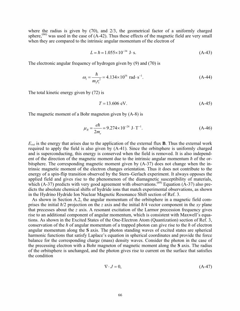
66

where the radius is given by (70), and 2/3, the geometrical factor of a uniformly charged sphere,(66) was used in the case of (A-42). Thus these effects of the magnetic field are very small when they are compared to the intrinsic angular momentum of the electron of 341.055 10 J s.L −= = × ⋅ (A-43) The electronic angular frequency of hydrogen given by (9) and (70) is

16 11 2

3 1

4.134 10 rad s .m r

ω −= = × ⋅ (A-44)

The total kinetic energy given by (72) is 13.606 eV.T = (A-45) The magnetic moment of a Bohr magneton given by (A-8) is

24 19.274 10 J T .2B

e

em

µ − −= = × ⋅ (A-46)

Erot is the energy that arises due to the application of the external flux B. Thus the external work required to apply the field is also given by (A-41). Since the orbitsphere is uniformly charged and is superconducting, this energy is conserved when the field is removed. It is also independ-ent of the direction of the magnetic moment due to the intrinsic angular momentum of the or-bitsphere. The corresponding magnetic moment given by (A-37) does not change when the in-trinsic magnetic moment of the electron changes orientation. Thus it does not contribute to the energy of a spin-flip transition observed by the Stern–Gerlach experiment. It always opposes the applied field and gives rise to the phenomenon of the diamagnetic susceptibility of materials, which (A-37) predicts with very good agreement with observations.(69) Equation (A-37) also pre-dicts the absolute chemical shifts of hydride ions that match experimental observations, as shown in the Hydrino Hydride Ion Nuclear Magnetic Resonance Shift section of Ref. 3.

As shown in Section A.2, the angular momentum of the orbitsphere in a magnetic field com-prises the initial /2 projection on the z axis and the initial /4 vector component in the xy plane that precesses about the z axis. A resonant excitation of the Larmor precession frequency gives rise to an additional component of angular momentum, which is consistent with Maxwell’s equa-tions. As shown in the Excited States of the One-Electron Atom (Quantization) section of Ref. 3, conservation of the of angular momentum of a trapped photon can give rise to the of electron angular momentum along the S axis. The photon standing waves of excited states are spherical harmonic functions that satisfy Laplace’s equation in spherical coordinates and provide the force balance for the corresponding charge (mass) density waves. Consider the photon in the case of the precessing electron with a Bohr magneton of magnetic moment along the S axis. The radius of the orbitsphere is unchanged, and the photon gives rise to current on the surface that satisfies the condition 0,J∇ ⋅ = (A-47)

67

corresponding to a rotating spherical harmonic dipole(70) that phase-matches the current (mass) density of (A-20). Thus the electrostatic energy is constant, and only the magnetic energy need be considered, as given by (A-50) to (A-52). The corresponding central field at the orbitsphere surface given by the superposition of the central field of the proton and that of the photon fol-lows from (2.10) to (2.17) of Ref 3:

00 12

0

[ ( , ) Re ( , ) ( )],4

ni tmr y

e Y Y e r rr

ωθ φ θ φ δπε

= + −E i i (A-48)

where the spherical harmonic dipole Y m(θ, φ) = sin θ is with respect to the S axis. The dipole spins about the S axis at the angular velocity given by (9). The resulting current is nonradiative, as shown in Section 6 and in Chapter 1, Appendix I, of Ref. 3. Thus the field in the RF rotating frame is magnetostatic, as shown in Fig. 6, but directed along the S axis. However, the precess-ing dipole results in magnetic dipole radiation or absorption during a Stern–Gerlach transition. The application of a magnetic field causes alignment of the intrinsic electron magnetic moment of atoms of a material such that the population of parallel versus antiparallel electrons is a Boltzmann distribution that depends on the temperature of the material. Following the removal of the field, the original random orientation distribution is restored, as is the original temperature. The distribution may be altered by the application of an RF pulse at the Larmor frequency.

The application of a magnetic field with a resonant Larmor excitation gives rise to a precessing angular momentum vector S of magnitude directed from the origin of the orbitsphere at an an-gle of θ = π/3 relative to the applied magnetic field. S rotates about the axis of the applied field at the Larmor frequency. The magnitude of the components of S that are parallel and orthogonal to the applied field (A-7b) and (A-7a) are /2 and 3 / 4 , respectively. Since both the RF field and the orthogonal components shown in Fig. 25 rotate at the Larmor frequency, the RF field that causes a Stern–Gerlach transition produces a stationary magnetic field with respect to these components, as described by Patz.(71)

The component of (A-7b) adds to the initial /2 parallel component to give a total of in the stationary frame corresponding to a Bohr magneton, µB, of magnetic moment. Equations (A-33) and (A-37) also hold in the case of the Stern–Gerlach experiment. Superposition holds for Max-well’s equations, and only the angular momentum given by (A-1) to (A-6) and the source current corresponding to (A-48) need be considered. Since it does not change, the diamagnetic compo-nent given by (A-32) does not contribute to the spin-flip transition, as discussed below. The po-tential energy of a magnetic moment m in the presence of flux B(64) is .E = ⋅m B (A-49) The angular momentum of the electron gives rise to a magnetic moment of µB. Thus the energy

spinmagE∆ to switch from parallel to antiparallel to the field is given by (A-66):

2 2 cos 2 .spin

mag B z B BE B Bµ µ θ µ∆ = ⋅ = =i B (A-50) In the case of an applied flux of 10 T, (A-50) gives 22 31.855 10 J 1.158 10 eV.spin

magE − −∆ = × = × (A-51)

68

spinmagE∆ is also given by Planck’s equation. It can be shown from conservation of angular momen-

tum considerations ((A-53) to (A-59)) that the Zeeman splitting is given by Planck’s equation and the Larmor frequency based on the gyromagnetic ratio (A-33). The electron’s magnetic mo-ment may only be parallel or antiparallel to the magnetic field rather than at a continuum of an-gles, including perpendicular, according to (A-49). No continuum of energies predicted by (A-49) for a pure magnetic dipole are possible. The energy difference for the magnetic moment to flip from parallel to antiparallel to the applied field is 22 32 1.855 10 J 1.158 10 eV,spin

magE ω − −∆ = = × = × (A-52) corresponding to magnetic dipole radiation.

As demonstrated in Section A.1, /2 of the orbitsphere angular momentum designated the static component is initially parallel to the field. An additional /2 parallel component designated the dynamic component comes from the of angular momentum along S. The angular momentum in the presence of an applied magnetic field is(72) ( ),em e= × +L r v A (A-53) where A is the vector potential evaluated at the location of the orbitsphere. The circular integral of A is the flux linked by the electron. During a Stern–Gerlach transition, a resonant RF photon is absorbed or emitted, and the component along S reverses direction. It is shown by (A-56) to (A-59) that the dynamic parallel component of angular momentum corresponding to the vector potential due to the light-like transition is equal to the “kinetic angular momentum” (r × mv) of /2. Conservation of angular momentum of the orbitsphere requires that the static angular mo-

mentum component concomitantly flip. The static component of angular momentum undergoes a spin-flip, and concomitantly the “potential angular momentum” (r × eA) of the dynamic compo-nent must change by – /2 due to the linkage of flux by the electron such that the total angular momentum is conserved.

In spherical coordinates the relationship between the vector potential A and the flux B is 22 .rA r Bπ π= (A-54) Equation (A-54) can be substituted into (A-53) since the magnetic moment m is given(64) as

charge angular momentum2 mass

m ⋅=

⋅ (A-55)

and the corresponding energy is consistent with (A-50) and (A-52) in this case as follows:

( ) / 2 .2 2 2

B

e e

e e em m

µ×∆ = − = =

r Am (A-56)

The boundary condition that the angular momentum is conserved is shown by (A-65) to (A-

67). It can be shown that (A-56) is also consistent with the vector potential along the axis of the applied field(72) given by

69

0 02 2

1cos sin sin .3 2 2 2e e

e em r m rφ φ

π µ θ µ θ= =A i i (A-57)

Substitution of (A-57) into (A-56) gives

0 2 2

0

1 sin2 2 1 ,2 2 2 2

e

e e e

ee em r e e

m m r m

φµ θµ

⎛ ⎞×⎜ ⎟ ⎛ ⎞⎝ ⎠∆ = − = − ⎜ ⎟

⎝ ⎠

r im (A-58)

with the geometrical factor of 2/3(66) and the current given by (A-20). Since k is the light-like k0, then k = ωn/c, corresponding to the RF photon field. The relativistic corrections of (A-58) are given by (1.218) and (1.219) of Ref. 3 and the relativistic radius r = C is given by (1.217) of Ref. 3. The relativistically corrected (A-58) is

2

1 0

0

1 (2 ) .2 2 2 2

B

e e

e em a mµ µπα

α− ⎛ ⎞

∆ = − =⎜ ⎟⎝ ⎠

m (A-59)

The magnetic flux of the electron is given by .∇× =A B (A-60) Substitution of (A-57) into (A-60) gives half the flux of the r > rn part of (A-26).

From (A-55), the /2 of angular momentum before and after the field is applied corresponds to an initial magnetic moment on the applied field axis of µB/2. After the field is applied, the con-tribution of µB/2 from (A-56) with (A-54) gives a total magnetic moment along the applied field axis of µB, a Bohr magneton, where the additional contribution (A-55) arises from the angular momentum of on the S axis. Thus, even though the magnitude of the vector projection of the angular momentum of the electron in the direction of the magnetic field is /2, the magnetic moment corresponds to due to the /2 contribution from the dynamic component, and the quan-tized transition is due to the requirement of angular momentum conservation as given by (A-55).

Equation (A-49) implies a continuum of energies; whereas (A-56) shows that the static-kinetic and dynamic vector potential components of the angular momentum are quantized at /2. Conse-quently, as shown in Section A.5, the flux linked during a spin transition is quantized as the magnetic flux quantum:

0 .2he

Φ = (A-61)

Only the states corresponding to

12sm = ± (A-62)

70

are possible due to conservation of angular momentum. It is further shown using the Poynting power vector, with the requirement that flux be linked in units of the magnetic flux quantum, that the factor 2 of (A-50) and (A-52) is replaced with the electron g factor. A.5 Electron g Factor

As demonstrated by Purcell,(62) when a magnetic field is applied to an electron in a central field that comprises a current loop, the orbital radius does not change, but the velocity changes as fol-lows:

.2 e

erBvm

∆ = (A-63)

This corresponds to diamagnetism and gives rise to precession with a corresponding resonance, as shown in Section A.4. The angular momentum in the presence of an applied magnetic field is(62) ( ),em e= × +L r v A (A-64) where A is the vector potential evaluated at the location of the orbitsphere. Conservation of an-gular momentum of the orbitsphere permits a discrete change of its kinetic angular momentum (r × mv) with respect to the field of /2, and concomitantly the potential angular momentum (r × eA) must change by – /2. The flux change φ of the orbitsphere for r < rn is determined as fol-lows:(62)

2 ˆ ˆ.2 2 2 2 2

e rA ee z zπ φπ π

⎛ ⎞ ⎛ ⎞∆ = − × = − = −⎜ ⎟ ⎜ ⎟⎝ ⎠ ⎝ ⎠

L r A (A-65)

In order that the change in angular momentum ∆L be equal to zero, φ must be Φ0 = h/2e, the

magnetic flux quantum. Thus, to conserve angular momentum in the presence of an applied magnetic field, the orbitsphere magnetic moment can be parallel or antiparallel to an applied field, as observed with the Stern–Gerlach experiment, and the flip between orientations is ac-companied by the “capture” of the magnetic flux quantum by the orbitsphere “coils” comprising infinitesimal loops of charge moving along great circles. A superconducting loop with a weak link also demonstrates this effect.(73)

The energy to flip the orientation of the orbitsphere due to its magnetic moment of a Bohr magneton µB is 2 ,spin

mag BE Bµ∆ = (A-66) where

.2B

e

em

µ = (A-67)

During the spin-flip transition, power must be conserved. Power flow is governed by the Poynting power theorem,

71

0 01 1( ) .2 2t t

µ ε∂ ∂⎛ ⎞ ⎛ ⎞∇ ⋅ × = − ⋅ − ⋅ − ⋅⎜ ⎟ ⎜ ⎟∂ ∂⎝ ⎠ ⎝ ⎠E H H H E E J E (A-68)

A.5.1 Stored Magnetic Energy

Energy superimposes; thus the calculation of the spin-flip energy is determined as a sum of contributions. The energy change corresponding to the “capture” of the magnetic flux quantum is derived below. From (A-31) for one electron,

2 2

00 2 3

12 ( )

fluxonmag

e n

eEm r

πµµ ⋅ = =H H (A-69)

is the energy stored in the magnetic field of the electron. The orbitsphere is equivalent to a Jo-sephson junction that can trap integer numbers of fluxons, where the quantum of magnetic flux is Φ0 = h/2e. Consider (A-69). During the flip transition, a fluxon treads the orbitsphere at the speed of light; therefore the radius of the orbitsphere in the lab frame is 2π times the relativistic radius in the fluxon frame, as shown in the Special Relativistic Correction to the Ionization En-ergies section of Ref. 3. Thus the energy of the transition corresponding to the “capture” of a fluxon by the orbitsphere, fluxon

magE , is

2 2 2 2

0 0 0 02 3 2 2 2 ,

( ) (2 ) 4 2 2 4fluxon

mag Be n e n e n e n

e e ee hEm r m r m e r m r A

πµ µ µ µπ π π π

⎛ ⎞⎛ ⎞ Φ⎛ ⎞= = =⎜ ⎟⎜ ⎟ ⎜ ⎟⎝ ⎠⎝ ⎠⎝ ⎠

(A-70)

where A is the area and Φ0 is the magnetic flux quantum. We have

2

02

12 ,2 4

fluxonmag B

e n

eE Bm r

µ µπ

⎛ ⎞= ⎜ ⎟

⎝ ⎠ (A-71)

where the nth fluxon treading through the area of the orbitsphere is equivalent to the applied magnetic flux. Furthermore, the term in brackets can be expressed in terms of the fine-structure constant α as follows:

2 2

0 0 .2 2e n e n

e e cvm r m vr c

µ µ= (A-72)

Substitution of (6) gives

2 2

0 0 .2 2e n

e e cvm r c

µ µ= (A-73)

Substitution of

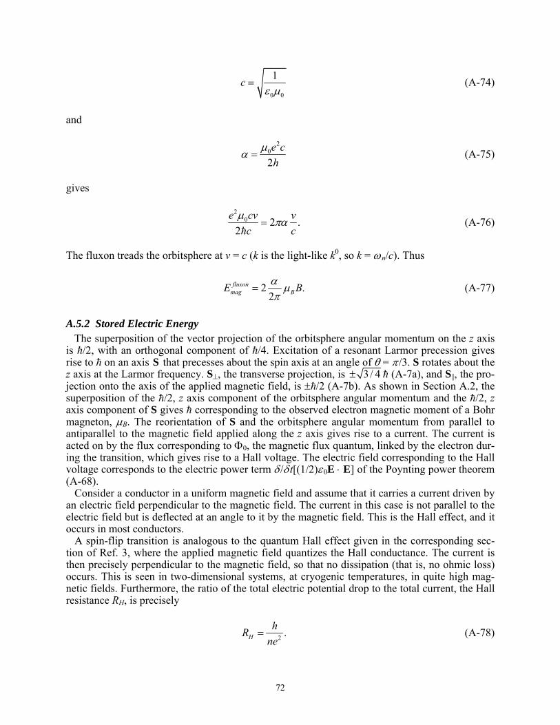
72

0 0

1cε µ

= (A-74)

and

2

0

2e ch

µα = (A-75)

gives

2

0 2 .2

e cv vc c

µ πα= (A-76)

The fluxon treads the orbitsphere at v = c (k is the light-like k0, so k = ωn/c). Thus

2 .2

fluxonmag BE Bα µ

π= (A-77)

A.5.2 Stored Electric Energy

The superposition of the vector projection of the orbitsphere angular momentum on the z axis is /2, with an orthogonal component of /4. Excitation of a resonant Larmor precession gives rise to on an axis S that precesses about the spin axis at an angle of θ = π /3. S rotates about the z axis at the Larmor frequency. S⊥, the transverse projection, is 3 / 4± (A-7a), and S||, the pro-jection onto the axis of the applied magnetic field, is ± /2 (A-7b). As shown in Section A.2, the superposition of the /2, z axis component of the orbitsphere angular momentum and the /2, z axis component of S gives corresponding to the observed electron magnetic moment of a Bohr magneton, µB. The reorientation of S and the orbitsphere angular momentum from parallel to antiparallel to the magnetic field applied along the z axis gives rise to a current. The current is acted on by the flux corresponding to Φ0, the magnetic flux quantum, linked by the electron dur-ing the transition, which gives rise to a Hall voltage. The electric field corresponding to the Hall voltage corresponds to the electric power term δ /δ t[(1/2)ε0E ⋅ E] of the Poynting power theorem (A-68).

Consider a conductor in a uniform magnetic field and assume that it carries a current driven by an electric field perpendicular to the magnetic field. The current in this case is not parallel to the electric field but is deflected at an angle to it by the magnetic field. This is the Hall effect, and it occurs in most conductors.

A spin-flip transition is analogous to the quantum Hall effect given in the corresponding sec-tion of Ref. 3, where the applied magnetic field quantizes the Hall conductance. The current is then precisely perpendicular to the magnetic field, so that no dissipation (that is, no ohmic loss) occurs. This is seen in two-dimensional systems, at cryogenic temperatures, in quite high mag-netic fields. Furthermore, the ratio of the total electric potential drop to the total current, the Hall resistance RH, is precisely

2 .HhR

ne= (A-78)

73

The factor n is an integer in the case of the integral quantum Hall effect and a small rational frac-tion in the case of the fractional quantum Hall effect. In an experimental plot(74) as a function of the magnetic field, the Hall resistance exhibits flat steps precisely at these quantized resistance values; however, the regular resistance vanishes (or is very small) at these Hall steps. Thus the quantized Hall resistance steps occur for a transverse superconducting state.

Consider the case that an external magnetic field is applied along the x axis to a two-dimensional superconductor in the yz plane that exhibits the integral quantum Hall effect (see Fig. 27). Conduction electrons align with the applied field in the x direction as the field perme-ates the material. The normal current carrying electrons experiences a Lorentzian force FL due to the magnetic flux. The y-directed Lorentzian force on an electron with velocity v in the z direc-tion by an x-directed applied flux B is .L e= ×F v B (A-79) The electron motion is a cycloid, where the center of mass experiences an E × B drift.(75) Conse-quently, the normal Hall effect occurs. Conduction electron energy states are altered by the ap-plied field and by the electric field corresponding to the Hall effect. The electric force FH due to the Hall electric field Ey is .H ye=F E (A-80) When these two forces are equal and opposite, conduction electrons propagate in the z direction alone. For this special case, it is demonstrated in Jackson(75) that the ratio of the corresponding Hall electric field EH to the applied magnetic flux is

,HE vB

= (A-81)

where v is the electron velocity. It is also demonstrated in the Integral Quantum Hall Effect sec-tion of Ref. 3 that the Hall resistance RH in the superconducting state is given by

2 ,HhR

ne= (A-82)

where n is an integer.

Consider the case of the spin-flip transition of the electron. In the case of an exact balance be-tween the Lorentzian force (A-79) and the electric force corresponding to the Hall voltage (A-80), each superconducting point mass of the electron propagates along a great circle, where

,E vB

= (A-83)

where v is given by (6). Substitution of (6) into (A-83) gives

74

.e

EB m r

= (A-84)

Equation (A-84) is the condition for superconductivity in the presence of crossed electric and magnetic fields. The electric field corresponding to the Hall voltage corresponds to the electric energy term Eele of the Poynting power theorem (A-68):

12

20

0 0 0

1 sin .2

r

eleE r drd dπ π

ε θ θ φ= ⋅∫ ∫ ∫ E E (A-85)

The electric term for this superconducting state is derived as follows using the coordinate system shown in Fig. 28.

The current is perpendicular to Er, so there is no dissipation. This occurs when e e= ×E v B (A-86) or

.E vB

= (A-87)

The electric field corresponding to the Hall voltage is .= ×E v B (A-88) Substitution of (A-88) into (A-85) gives

12

2 20

0 0 0

1 ( ) sin .2

r

eleE vB r drd dπ π

ε θ θ φ= ∫ ∫ ∫ (A-89)

The spin-flip transition may be induced by the absorption of a resonant photon. The velocity is determined from the distance traversed by each point and the time of the transition due to capture of a photon resonant with the spin-flip transition energy. The current iφ corresponding to the Hall voltage and Er is given by the product of the electron charge and the frequency f of the photon, where the correspondence principle holds, as given in the Photon Absorption section of Ref. 3: .i ef= (A-90) The resistance of free space for the propagation of a photon is the radiation resistance of free space η:

0

0

.µηε

= (A-91)

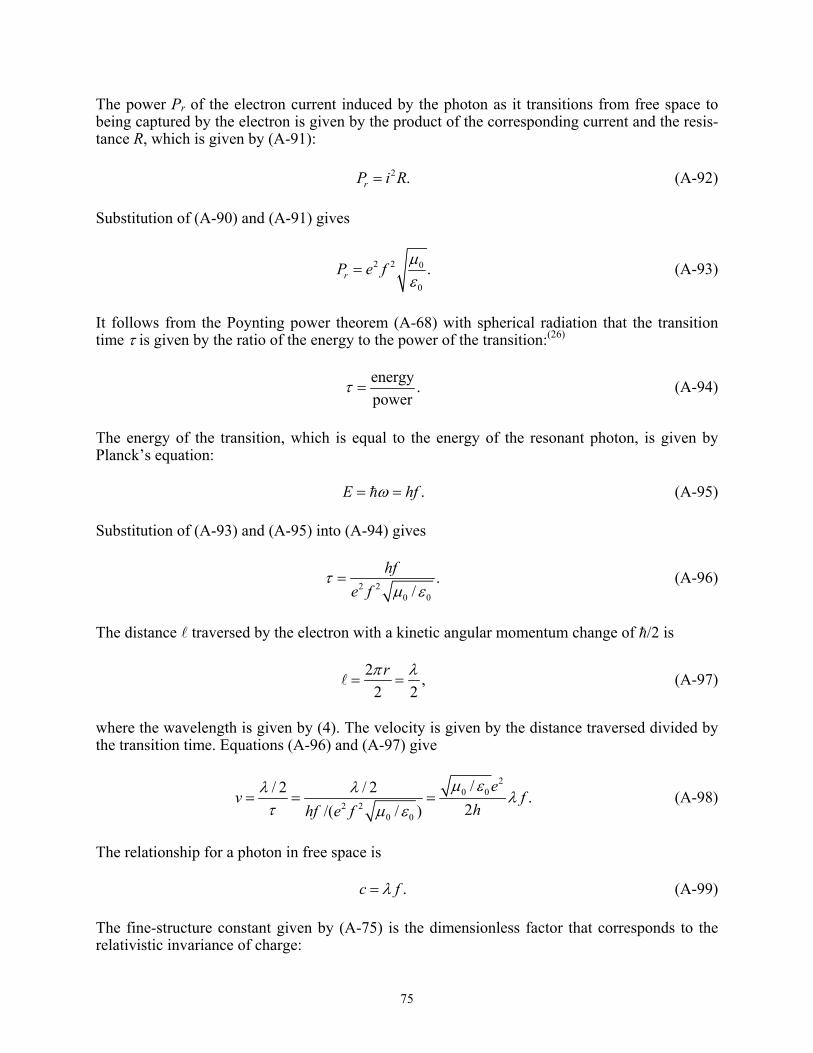
75

The power Pr of the electron current induced by the photon as it transitions from free space to being captured by the electron is given by the product of the corresponding current and the resis-tance R, which is given by (A-91): 2 .rP i R= (A-92) Substitution of (A-90) and (A-91) gives

2 2 0

0

.rP e f µε

= (A-93)

It follows from the Poynting power theorem (A-68) with spherical radiation that the transition time τ is given by the ratio of the energy to the power of the transition:(26)

energy .power

τ = (A-94)

The energy of the transition, which is equal to the energy of the resonant photon, is given by Planck’s equation: .E hfω= = (A-95) Substitution of (A-93) and (A-95) into (A-94) gives

2 2

0 0

./

hfe f

τµ ε

= (A-96)

The distance traversed by the electron with a kinetic angular momentum change of /2 is

2 ,2 2

rπ λ= = (A-97)

where the wavelength is given by (4). The velocity is given by the distance traversed divided by the transition time. Equations (A-96) and (A-97) give

2

0 02 2

0 0

// 2 / 2 .2/( / )

ev f

hhf e fµ ελ λ λ

τ µ ε= = = (A-98)

The relationship for a photon in free space is .c fλ= (A-99) The fine-structure constant given by (A-75) is the dimensionless factor that corresponds to the relativistic invariance of charge:

76

22

0 00 02

0

/1 1 .4 2 / 2

e ceh e hµ εµ µα

π ε= = = (A-100)

It is equivalent to one half the ratio of the radiation resistance of free space, 0 0/µ ε , to the Hall resistance h/e2. The radiation resistance of free space is equal to the ratio of the electric field and the magnetic field of the photon (113). Substitution of (A-99) and (A-100) into (A-98) gives .v cα= (A-101) Substitution of (A-101) into (A-89) gives

122 2

0 00 0 0

1 ( ) sin ,2

r

eleE c H r drd dπ π

ε α µ θ θ φ= ∫ ∫ ∫ (A-102)

where 0 .B Hµ= (A-103) The relationship between the speed of light c and the permittivity of free space ε0 and the perme-ability of free space µ0 is

0 0

1 .cµ ε

= (A-104)

Thus (A-102) may be written as

12

2 2 20

0 0 0

1 sin .2

r

eleE H r drd dπ π

α µ θ θ φ= ∫ ∫ ∫ (A-105)

Substitution of (A-29) gives

2 2

2 02 3

1

2 .3ele

e

eEm r

πµα= (A-106)

The magnetic flux B is quantized in terms of the Bohr magneton because the electron links flux in units of the magnetic flux quantum

0 .2he

Φ = (A-107)

Substitution of (A-69) to (A-77) gives

77

222 .3 2ele BE Bαα µ

π⎛ ⎞= ⎜ ⎟⎝ ⎠

(A-108)

A.5.3 Dissipated Energy

The J ⋅ E energy over time is derived from the electron current corresponding to the Larmor excitation and the electric field given by Faraday’s law due to the linkage of the magnetic flux of the fluxon during the spin-flip. Consider the electron current due to the external field. The appli-cation of a magnetic field with a resonant Larmor excitation gives rise to a precessing angular momentum vector S of magnitude directed from the origin of the orbitsphere at an angle of θ = π /3 relative to the applied magnetic field. As given in Section A.2, S rotates about the axis of the applied field at the Larmor frequency. The magnitude of the components of S that are parallel and orthogonal to the applied field (A-7b) and (A-7a) are /2 and 3/ 4 , respectively. Since both the RF field and the orthogonal components shown in Fig. 25 rotate at the Larmor fre-quency, the RF field that causes a Stern–Gerlach transition produces a stationary magnetic field with respect to these components, as described in Section A.4. The corresponding central field at the orbitsphere surface given by the superposition of the central field of the proton and that of the photon follows from (2.10) to (2.17) of Ref. 3 and is given by (A-48):

00 12

0

[ ( , ) Re ( , ) ( )],4

ni tmr y

e Y Y e r rr

ωθ φ θ φ δπε

= + −E i i (A-109)

where the spherical harmonic dipole Y m(θ, φ) = sin θ is with respect to the S axis. The dipole spins about the S axis at the angular velocity given by (9). The resulting current is nonradiative, as shown in Section 6. Thus the field in the RF is magnetostatic, as shown in Fig. 6, but directed along the S axis. Thus the corresponding current given by (A-17) is

3

3( , , ) sin .2 e n

ezm r φρ φ θ=K i (A-110)

Next consider Faraday’s equation for the electric field:

0 .C S

dd ddt

µ⋅ = − ⋅∫ ∫E s H a (A-111)

As demonstrated by Purcell,(62) the velocity of the electron changes according to Lenz’s law, but the change in centrifugal force is balanced by the change in the central field due to the applied field. The magnetic flux of the electron given by (A-26) is

00 3

1

( cos sin ) for .r ne

e r rm r θµµ θ θ= = − <B H i i (A-112)

From (A-77) the magnetic flux BJ⋅E of the fluxon is

0 03 3

1 1

( cos sin ) .2 2r z

e e

e em r m rθµ µα αθ θ

π π⋅ = − =J EB i i i (A-113)

78

The electric field E is constant about the line integral of the orbitsphere. Using (A-111) with the change in flux in units of fluxons along the z axis given by (A-113) gives

1 1

1 1

2 ,r r

r C r

dBd dz r dzdt φπ

+ +

− −

⋅ = −∫ ∫ ∫E s i (A-114)

2 2 3 21 1 1

0

22 sin sin .3

B Br d r d rt t

π

φ φπ θ θ π θ θ π∆ ∆= − = −

∆ ∆∫E i i (A-115)

Substitution of (A-113) into (A-115) gives

2 0 01 1 3

1 1

2 2 .3 2 3 2e e

e er rm r t m r tφ φµ µα απ π π

π π= − = −

∆ ∆E i i (A-116)

Thus

02

1

2 .3 2 e

em r t φµα

π= −

∆E i (A-117)

The dissipative power density E ⋅ J can be expressed in terms of the surface current density K as ( ) ( ) .

V S

tdv tda⋅ ∆ = ⋅ ∆∫ ∫E J E K (A-118)

Using the electric field from (A-117) and the current density from (A-110) gives

2 2 220 0

12 3 2 31 1 10 0

2 3 4( ) sin .3 2 2 3 2e e eV

e eetdv tr d dm r t m r m r

π π µ πµα αθ θ ϕπ π

⎛ ⎞⋅ ∆ = ∆ =⎜ ⎟∆⎝ ⎠

∫ ∫ ∫E J (A-119)

Substitution of (A-77) into (A-119) gives

24( ) 2 .

3 2 BV

tdv Bα µπ

⎛ ⎞⎛ ⎞⋅ ∆ = ⎜ ⎟⎜ ⎟⎝ ⎠⎝ ⎠∫ E J (A-120)

A.5.4 Total Energy of Spin-Flip Transition

The principal energy of the transition corresponding to a reorientation of the orbitsphere is given by (A-66). The total energy of the flip transition is the sum of (A-66) with (A-77), (A-108), and (A-120) corresponding to the electric energy, the magnetic energy, and the dissipated energy of a fluxon treading the orbitsphere, respectively:

79

2

22 42 1 ,2 3 2 3 2

spinmag B BE B g Bα α αα µ µ

π π π⎛ ⎞⎛ ⎞ ⎛ ⎞∆ = + + − =⎜ ⎟⎜ ⎟ ⎜ ⎟⎜ ⎟⎝ ⎠ ⎝ ⎠⎝ ⎠

(A-121)

where the stored magnetic energy corresponding to the ∂/∂t[(1/2)µ0H ⋅ H] term increases, the stored electric energy corresponding to the ∂/∂t[(1/2)ε0E ⋅ E] term increases, and the J ⋅ E term is dissipative. The magnetic moment of (A-66) is twice that from the gyromagnetic ratio, as given by (A-55). The magnetic moment of the electron is the sum of the component corresponding to the kinetic angular momentum /2 and the component corresponding to the vector potential an-gular momentum /2 (A-64). The spin-flip transition can be considered as involving a magnetic moment of g times that of a Bohr magneton. The g factor is redesignated the fluxon g factor as opposed to the anomalous g factor, and it is given by (A-121):

2

22 41 .2 2 3 2 3 2g α α αα

π π π⎛ ⎞ ⎛ ⎞= + + −⎜ ⎟ ⎜ ⎟⎝ ⎠ ⎝ ⎠

(A-122)

For α–1 = 137.036 04(11),(76)

1.001 159 652 120.2g

= (A-123)

The experimental value(23) is

1.001 159 652 188(4).2g

= (A-124)

The calculated and experimental values are within the propagated error of the fine-structure con-stant. Different values of the fine-structure constant have been recorded from different experi-mental techniques, and α–1 depends on a circular argument between theory and experiment.(39) One measurement of the fine-structure constant based on the electron g factor is 1

egα − = 137.036 006(20).(77) This value can be contrasted with equally precise measurements employing solid state techniques such as those based on the Josephson effect(78) (αJ

–1 = 137.035 963(15)) or the quantized Hall effect(79) (αH

–1 = 137.035 300(400)). A method of determination of α–1 that depends on the circular methodology between theory and experiment to a lesser extent is the substitution of the independently measured fundamental constants µ0, e, c, and h into (A-100). The following values of the fundamental constants are given by Weast:(76) 7 1

0 4 10 Hm ,µ π − −= × (A-125) 191.602 189 2(46) 10 C,e −= × (A-126) 82.997 924 58(12) 10 m/s,c = × (A-127) 34 16.626 176(36) 10 J Hz .h − −= × ⋅ (A-128)

80

For these constants, 1 137.036 03(82).α − = (A-129) Substitution of the α–1 from (A-129) into (A-122) gives

1.001 159 652 137.2g

= (A-130)

The experimental value(23) is

1.001 159 652 188(4).2g

= (A-131)

The postulated QED theory of g/2 is based on the determination of the terms of a postulated

power series in α /π, where each postulated virtual particle is a source of postulated vacuum po-larization that gives rise to a postulated term. The algorithm involves scores of postulated Feyn-man diagrams corresponding to thousands of matrices with thousands of integrations per matrix requiring decades to reach a consensus on the “appropriate” postulated algorithm to remove the intrinsic infinities. The remarkable agreement between (A-130) and (A-131) demonstrates that g/2 may be derived in closed form from Maxwell’s equations in a simple straightforward manner that yields a result with 11-figure agreement with experiment — the limit of the experimental capability of the measurement of α directly or the fundamental constants to determine α. In Chapter 1, Appendix II, of Ref. 3, the Maxwellian result is contrasted with the QED algorithm of invoking virtual particles, zero-point fluctuations of the vacuum, and negative energy states of the vacuum. Rather than an infinity of radically different QED models, an essential feature is that Maxwellian solutions are unique.

Endnotes 1 The orbitsphere has zero thickness, but in order for the speed of light to be a constant maxi-

mum in any frame including that of the gravitational field that propagates out as a light-wave front at particle production, it gives rise to a space-time dilation equal to 2π times the Newto-nian gravitational or Schwarzschild radius rg = 2Gme/c2 = 1.3525 × 10–57 m according to (170) and (194). This corresponds to a space-time dilation of 8.4980 × 10–57 m or 2.8346 × 10–65 s. Although the orbitsphere does not occupy space in the third spatial dimension, its mass discon-tinuity effectively “displaces” space-time, where the space-time dilation can be considered as a “thickness” associated with its gravitational field.

2 The theories of Bohr, Schrödinger, and now CQM all give the identical equation for the princi-pal energy levels of the hydrogen atom:

2 2 2

18 22 2 2

0

13.5982.1786 10 J eV.8ele

H

Z e ZE Zn a n nπε

−= − = − × × = − ×

(N-1)

81

In CQM, the two-dimensional wave equation is solved for the charge density function of the electron. And, the Fourier transform of the charge density function is a solution of the three-dimensional wave equation in frequency (k, ω) space. However, the Schrödinger equation solu-tions are three-dimensional in space-time. The energy is given by

2 ,H dv E dvψ ψ ψ∞ ∞

−∞ −∞

=∫ ∫ (N-2)

2 1.dvψ∞

−∞

=∫ (N-3)

Thus

.H dv Eψ ψ∞

−∞

=∫ (N-4)

In the case that the potential energy of the Hamiltonian H is a constant times the wave-number,

the Schrödinger equation is the well-known Bessel equation. Then with one of the solutions for ψ, (N-4) is equivalent to an inverse Fourier transform. According to the duality and scale change properties of Fourier transforms, the energy equation of CQM and that of QM are iden-tical, i.e., the energy of a radial Dirac delta function of radius equal to an integer multiple of the radius of the hydrogen atom (N-1). Bohr obtained the same energy formula by postulating nonradiative states with angular momentum

zL m= (N-5)

and solving the energy equation classically. The mathematics for all three theories converge to (N-1). However, the physics is quite dif-

ferent. Only CQM is derived from first principles and holds over a scale of space-time of 85 orders of magnitude. And, the mathematical relationship of CQM and QM is based on the Fou-rier transform of the radial function. CQM requires that the electron be real and physically con-fined to a two-dimensional surface that corresponds to a solution of the two-dimensional wave equation plus time. The corresponding Fourier transform is a wave over all space that is a solu-tion of the three-dimensional wave equation (e.g., the Schrödinger equation). In essence QM may be considered as a theory dealing with the Fourier transform of an electron rather than the physical electron. By Parseval’s theorem the energies may be equivalent, but the quantum-mechanical case is nonphysical — only mathematical. Thus it is nonsensical from this perspec-tive. It may mathematically produce numbers that agree with experimental energies, but the mechanisms lack internal consistency and conformity with physical laws. If these are the crite-ria for a valid solution of physical problems, then QM has never successfully solved any prob-lem. The theory of Bohr similarly failed.

Classical revisions may transform Schrödinger’s and Heisenberg’s quantum theory into what is termed a classical quantum theory such that physical descriptions result. For example, in the old quantum theory the spin angular momentum of the electron is called the “intrinsic angular momentum.” This term arises because it is difficult to provide a physical interpretation for the electron’s spin angular momentum. QED provides somewhat of a physical interpretation by

82

proposing that the “vacuum” contains fluctuating electric and magnetic fields. In contrast, in CQM, spin angular momentum results from the motion of negatively charged mass moving systematically, and the equation for angular momentum r × p can be applied directly to the wave-function (a current density function) that describes the electron. And, quantization is car-ried by the photon, rather than probability waves of the electron, as demonstrated in this paper.

3 The second is currently defined as the time required for 9 192 631 770 vibrations within the cesium-133 atom. The “sec” as defined in (179) is a fundamental constant, namely the metric of space-time (it is almost identically equal to the present value for reasons explained in Ref. 3). A unified theory can only provide the relationships between all measurable observables in terms of a clock defined in terms of fundamental constants according to those observables and used to measure them. The so-defined “clock” measures “clicks” on an observable in one as-pect, and in another, it is the ruler of space-time of the universe with the implicit dependence of space-time on matter-energy conversion, as shown in Section 29.

4 The torque balance can be appreciated by considering that S is aligned with ZR if the XR com-ponent is zero, and the three vectors are mutually orthogonal if the XR component is /2. The balance can be shown by considering the magnetic energies resulting from the corresponding torques when they are balanced. Using (A-50) and (A-52), the potential energy EV due to the projection of S’s angular momentum of along ZR with /2 of angular momentum is

1 1cos cos cos ,2 2B BV B BE B Bµ µµ θ µ θ ω θ= = = (N-6)

where

BBµ is the flux due to a magnetic moment of a Bohr magneton and

Bµω is the corre-sponding gyromagnetic frequency. The application of a magnetic moment along the XR axis causes S to precess about the ZR and XR axes. In the XRYRZR frame rotating at

Bµω , S precesses about the XR axis. The corresponding precession energy

RXE of S about the XR component of /4 is the corresponding Larmor energy

1 .4R BXE µω= − (N-7)

The energy

RZE of the magnetic moment corresponding to S rotating about ZR with /2 of an-gular momentum is the corresponding Larmor energy

1 .2R BZE µω= (N-8)

At torque balance the potential energy is equal to the sum of the Larmor energies:

1 1 1/ 4 11 cos .2 4 2 1/ 2 2R R B B BZ XE E µ µ µω ω ω θ⎛ ⎞ ⎛ ⎞+ = − = − =⎜ ⎟ ⎜ ⎟

⎝ ⎠ ⎝ ⎠ (N-9)

Balance occurs when θ = π /3. Thus the intrinsic torques are balanced. Furthermore, energy is

conserved relative to the external field as well as the intrinsic ZR and XR components of the or-bitsphere, and the Larmor relationships for both the gyromagnetic ratio and the potential en-ergy of the resultant magnetic moment are satisfied, as shown in Section A.4.

5 As shown in Section A.4, the angular momentum of on the S axis is due to a photon standing

83

wave that is phase-matched to a spherical harmonic source current, i.e., a spherical harmonic dipole Y m(θ, φ) = sin θ with respect to the S axis. The dipole spins about the S axis at the angu-lar velocity given by (9). Since the field is magnetostatic in the RF rotating frame, the current is equivalent to current loops along the S axis. Thus the derivation of the corresponding mag-netic field is the same as that of the stationary field given in this section.

References 1. F. Laloë, Am. J. Phys. 69, 655 (2001). 2. G. Landvogt, Internat. J. Hydrogen Energy 28, 1155 (2003). 3. R.L. Mills, The Grand Unified Theory of Classical Quantum Mechanics, May 2005 Edition,

BlackLight Power, Inc., Cranbury, NJ. Available at http://www.blacklight-power.com/book.shtml.

4. Idem, Internat. J. Hydrogen Energy 25, 1171 (2000). 5. Ibid. 26, 1059 (2001). 6. H. Margenau and G.M. Murphy, The Mathematics of Physics and Chemistry, 2nd edition

(D. Van Nostrand, New York, 1956), pp. 363–367. 7. H.J. Maris, J. Low Temp. Phys. 120, 173 (2000). 8. C.A. Fuchs and A. Peres, Phys. Today 53, 70 (2000). 9. S. Peil and G. Gabrielse, Phys. Rev. Lett. 83, 1287 (1999). 10. F.J. Dyson, Am. J. Phys. 58, 209 (1990). 11. J. Horgan, Sci. Am. 267, 94 (1992). 12. H.A. Haus, Am. J. Phys. 54, 1126 (1986). 13. R.L. Mills, Global Foundation, Inc., Orbis Scientiae, in The Role of Attractive and Repulsive

Gravitational Forces in Cosmic Acceleration of Particles. The Origin of the Cosmic Gamma Ray Bursts, 29th Conference on High Energy Physics and Cosmology Since 1964, Dr. Behram N. Kursunoglu, Chairman, 14–17 December 2000, Lago Mar Resort, Fort Lauder-dale, FL (Kluwer Academic/Plenum Publishers, New York), pp. 243–258.

14. Idem, Internat. J. Hydrogen Energy 27, 565 (2002). 15. D.A. McQuarrie, Quantum Chemistry (University Science Books, Mill Valley, CA, 1983),

pp. 206–225. 16. J. Daboul and J.H.D. Jensen, Z. Phys. 265, 455 (1973). 17. T.A. Abbott and D.J. Griffiths, Am. J. Phys. 53, 1203 (1985). 18. G. Goedecke, Phys. Rev. B 135, 281 (1964). 19. P. Pearle, Found. Phys. 7, 931 (1977). 20. L.C. Shi and J.A. Kong, Applied Electromagnetism (Brooks/Cole Engineering Division,

Monterey, CA, 1983), pp. 170–209. 21. J.D. Jackson, Classical Electrodynamics, 2nd edition (John Wiley & Sons, New York,

1975), pp. 739–779. 22. Ref. 15, pp. 238–241. 23. R.S. Van Dyck, Jr., P. Schwinberg, and H. Dehmelt, Phys. Rev. Lett. 59, 26 (1987). 24. M. Mizushima, Quantum Mechanics of Atomic Spectra and Atomic Structure (W.A. Benja-

min, Inc., New York, 1970), p. 17. 25. Ref. 21, pp. 739–752. 26. Ibid., pp. 758–763. 27. E.M. Purcell, Electricity and Magnetism (McGraw-Hill, New York, 1965), pp. 156–167. 28. D. Clark, J. Chem. Educ. 68, 454 (1991). 29. J. Gribbin, New Scientist, 153, 2066 (1997). 30. I. Levine et al., Phys. Rev. Lett. 78, 424 (1997).

84

31. C.E. Moore, “Ionization Potentials and Ionization Limits Derived from the Analyses of Op-tical Spectra,” Nat. Stand. Ref. Data Ser.-Nat. Bur. Stand. (U.S.), No. 34, 1970.

32. R.C. Weast, CRC Handbook of Chemistry and Physics, 58th edition (CRC Press, West Palm Beach, FL, 1977), p. E-68.

33. P.J. Bromberg, J. Chem. Phys. 50, 3906 (1969). 34. J. Geiger, Z. Phys. 175, 530 (1963). 35. A. Beiser, Concepts of Modern Physics, 4th edition (McGraw-Hill, New York, 1978), pp. 2–

10. 36. E.G. Adelberger, C.W. Stubbs, B.R. Heckel, Y. Su, H.E. Swanson, G. Smith, and J.H.

Gundlach, Phys. Rev. D 42, 3267 (1990). 37. G.R. Fowles, Analytical Mechanics, 3rd edition (Holt, Rinehart, and Winston, New York,

1977), pp. 154–155. 38. K. Hagiwara et al., Phys. Rev. D 66, 010001 (2002). Also available at http://pdg.lbl.gov/

2002/s035.pdf. 39. P.J. Mohr and B.N. Taylor, Rev. Modern Phys. 72, 351 (2000). 40. T. Van Flandern, Phys. Lett. A 250, 1 (1998). 41. R. Cowen, Sci. News 153, 292 (1998). 42. M. Chown, New Scientist 154, 50 (1997). 43. B. Schwarzschild, Phys. Today 51, 19 (1998). 44. J.C. Mather and E.S. Cheng, Astrophys. J. Lett. 354, L37 (1990). 45. W. Saunders and C. Frenk, Nature 349, 32 (1991). 46. R.P. Kirshner, A. Oemler, Jr., P.L. Schechter, and S.A. Shectman, Astron. J. 88, 1285

(1983). 47. V. de Lapparent, M.J. Geller, and J.P. Huchra, Astrophys. J. 332, 44 (1988). 48. A. Dressler, S.M. Faber, D. Burstein, R.L. Davies, D. Lynden-Bell, R.J. Terlevich, and G.

Wegner, Astrophys. J. 313, L37 (1987). 49. S. Flamsteed, Discover 16, 66 (1995). 50. J. Glanz, Science 273, 581 (1996). 51. S.D. Landy, Sci. Am. 280, 38 (1999). 52. W.L. Freeman, B.F. Madore, and G.D. Illingworth, Nature 371, 757 (1994). 53. R.M. Wald, General Relativity (University of Chicago Press, Chicago, 1984), pp. 114–116. 54. P.J.E. Peebles and J. Silk, Nature 346, 233 (1990). 55. W. McC. Siebert, Circuits, Signals, and Systems (The MIT Press, Cambridge, MA, 1986),

pp. 597–603. 56. J. Glanz, Science 279, 1298 (1998). 57. R. Cowen, Sci. News 153, 344 (1998). 58. Ibid. 154, 277 (1998). 59. P. de Bernardis et al., Nature 404, 955 (2000). Also available at http://www.phys.cwru.edu/

boomerang/papers.html/debernardis00.pdf. 60. N.W. Halverson, E.M. Leitch, C. Pryke, J. Kovac, J.E. Carlstrom, W.L. Holzapfel, M.

Dragovan, J.K. Cartwright, B.S. Mason, S. Padin, T.J. Pearson, M.C. Shepard, and A.C.S. Readhead, “DASI First Results: A Measurement of the Cosmic Microwave Background An-gular Power Spectrum,” arXiv:astro-ph/0104489, 30 April 2001.

61. B. Holverstott and R. Mills, “Modeling the Orbitsphere.” Available at http://www.blacklight power.com/pdf/technical/animations/Appendix%20III%20-%20Orbitsphere%20020905.pdf.

62. Ref. 27, pp. 370–375, 447. 63. R.L. Mills, “The Fallacy of Feynman’s Argument on the Stability of the Hydrogen Atom

According to Quantum Mechanics,” submitted. 64. Ref. 15, pp. 238–241.

85

65. Ref. 21, p. 178. 66. Ref. 37, p. 196. 67. Ref. 15, pp. 206–221. 68. Ref. 21, pp. 194–197. 69. Ref. 27, pp. 370–379. 70. Ref. 21, pp. 84–102; 752–763. 71. S. Patz, Cardiovasc. Interven. Radiol. 8(25), 225 (1986). 72. Ref. 27, pp. 361–367. 73. C.E. Gough, M.S. Colclough, E.M. Forgan, R.G. Jordan, M. Keene, C.M. Muirhead, A.I.M.

Rae, N. Thomas, J.S. Abell and S. Sutton, Nature 326, 855 (1987). 74. S. Das Sarma and R.E. Prange, Science 256, 1284 (1992). 75. Ref. 21, pp. 582–584. 76. R.C. Weast, CRC Handbook of Chemistry and Physics, 68th Edition (CRC Press, Boca

Raton, FL, 1987–88), pp. F-186–F-187. 77. G.P. Lepage, Proceedings of the International Conference on Atomic Physics (World Scien-

tific, Singapore, 1981), p. 297. 78. E.R. Williams and P.T. Olsen, Phys. Rev. Lett. 42, 1575 (1979). 79. K.V. Klitzing, G. Dorda, and M. Pepper, Phys. Rev. Lett. 45, 494 (1980).

86

Table I: The Calculated Electric (per electron), Magnetic (per electron), and Ionization Energies for Some Two-Electron Atoms Atom r1

(a0)a Electric

Energyb (eV) Magnetic

Energyc (eV) Calculated Ionization

Energyd (eV) Experimental

Ionization(31,32) Energy (eV) He 0.567 –23.96 0.63 24.59 24.59 Li+ 0.356 –76.41 2.54 75.56 75.64 Be2+ 0.261 –156.08 6.42 154.48 153.89 B3+ 0.207 –262.94 12.96 260.35 259.37 C4+ 0.171 –396.98 22.83 393.18 392.08 N5+ 0.146 –558.20 36.74 552.95 552.06 O6+ 0.127 –746.59 55.35 739.67 739.32 F7+ 0.113 –962.17 79.37 953.35 953.89 a from (130) b from (132) c from (133) d from (131) and (134)

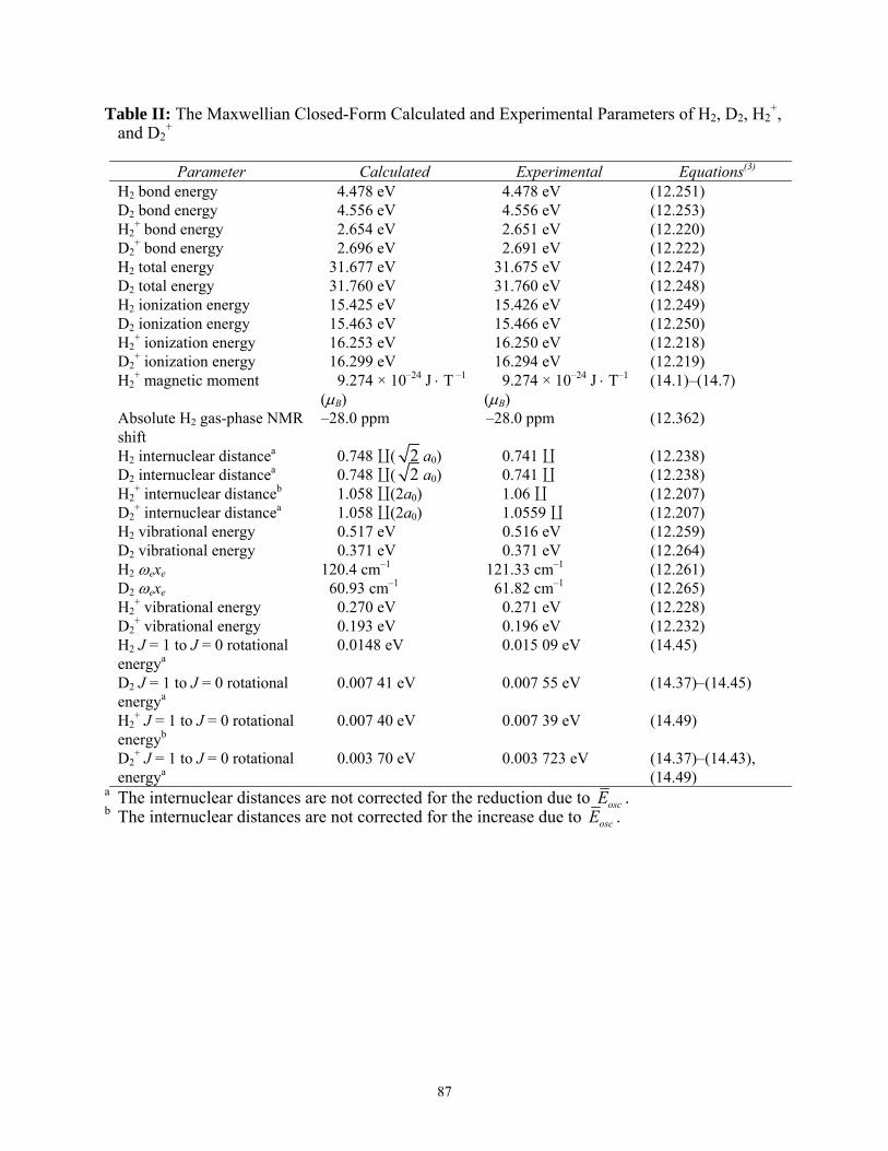
87

Table II: The Maxwellian Closed-Form Calculated and Experimental Parameters of H2, D2, H2+,

and D2+

Parameter Calculated Experimental Equations(3)

H2 bond energy 4.478 eV 4.478 eV (12.251) D2 bond energy 4.556 eV 4.556 eV (12.253) H2

+ bond energy 2.654 eV 2.651 eV (12.220) D2

+ bond energy 2.696 eV 2.691 eV (12.222) H2 total energy 31.677 eV 31.675 eV (12.247) D2 total energy 31.760 eV 31.760 eV (12.248) H2 ionization energy 15.425 eV 15.426 eV (12.249) D2 ionization energy 15.463 eV 15.466 eV (12.250) H2

+ ionization energy 16.253 eV 16.250 eV (12.218) D2

+ ionization energy 16.299 eV 16.294 eV (12.219) H2

+ magnetic moment 9.274 × 10–24 J ⋅ T –1 (µB)

9.274 × 10–24 J ⋅ T–1 (µB)

(14.1)–(14.7)

Absolute H2 gas-phase NMR shift

–28.0 ppm –28.0 ppm (12.362)

H2 internuclear distancea 0.748 ( 2 a0) 0.741 (12.238) D2 internuclear distancea 0.748 ( 2 a0) 0.741 (12.238) H2

+ internuclear distanceb 1.058 (2a0) 1.06 (12.207) D2

+ internuclear distancea 1.058 (2a0) 1.0559 (12.207) H2 vibrational energy 0.517 eV 0.516 eV (12.259) D2 vibrational energy 0.371 eV 0.371 eV (12.264) H2 ωexe 120.4 cm–1 121.33 cm–1 (12.261) D2 ωexe 60.93 cm–1 61.82 cm–1 (12.265) H2

+ vibrational energy 0.270 eV 0.271 eV (12.228) D2

+ vibrational energy 0.193 eV 0.196 eV (12.232) H2 J = 1 to J = 0 rotational energya

0.0148 eV 0.015 09 eV (14.45)

D2 J = 1 to J = 0 rotational energya

0.007 41 eV 0.007 55 eV (14.37)–(14.45)

H2+ J = 1 to J = 0 rotational

energyb 0.007 40 eV 0.007 39 eV (14.49)

D2+ J = 1 to J = 0 rotational

energya 0.003 70 eV 0.003 723 eV (14.37)–(14.43),

(14.49) a The internuclear distances are not corrected for the reduction due to oscE . b The internuclear distances are not corrected for the increase due to oscE .

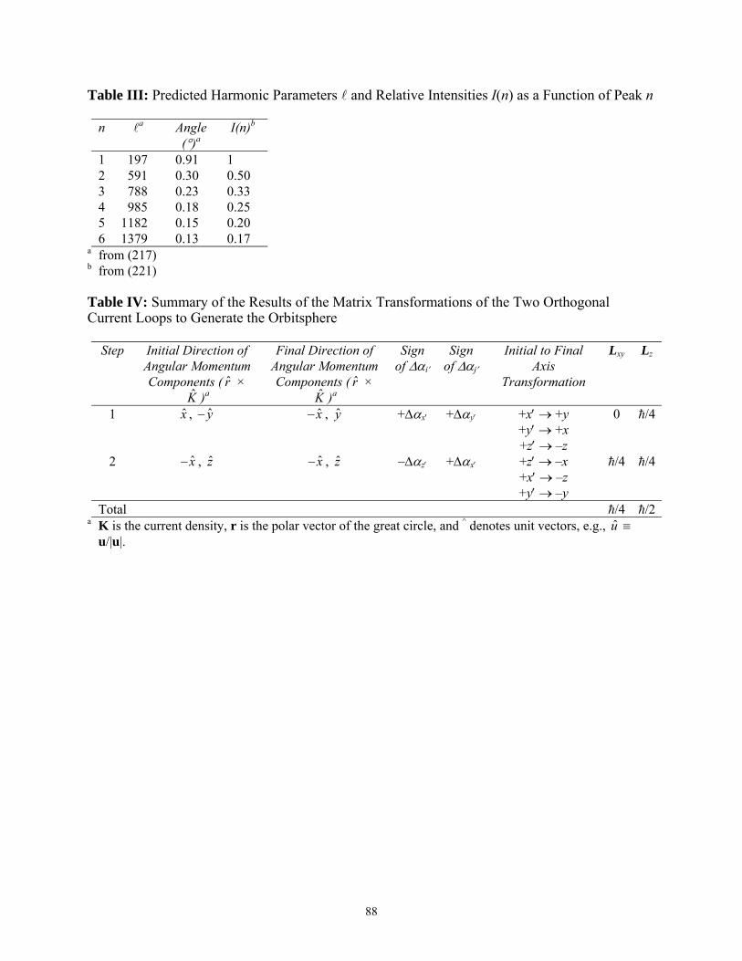
88

Table III: Predicted Harmonic Parameters and Relative Intensities I(n) as a Function of Peak n

n a Angle (°)a

I(n)b

1 197 0.91 1 2 591 0.30 0.50 3 788 0.23 0.33 4 985 0.18 0.25 5 1182 0.15 0.20 6 1379 0.13 0.17

a from (217) b from (221) Table IV: Summary of the Results of the Matrix Transformations of the Two Orthogonal Current Loops to Generate the Orbitsphere

Step Initial Direction of Angular Momentum Components ( r ×

K )a

Final Direction of Angular Momentum Components ( r ×

K )a

Sign of ∆αi′

Sign of ∆αj′

Initial to Final Axis

Transformation

Lxy Lz

1 x , y− x− , y +∆αx′ +∆αy′ +x′ → +y +y′ → +x +z′ → –z

0 /4

2 x− , z x− , z –∆αz′ +∆αx′ +z′ → –x +x′ → –z +y′ → –y

/4 /4

Total /4 /2a K is the current density, r is the polar vector of the great circle, and ^ denotes unit vectors, e.g., u ≡

u/|u|.

89

Figure 1. The orbitsphere is a two-dimensional spherical shell of zero thickness with the Bohr radius of the hydrogen atom, r = a H.

90

Fig. 2. The current pattern of the orbitsphere shown with 6 degree increments of the infinitesi-mal angular variables ±∆αi' and ±∆α j ' from the perspective of looking along the z-axis. The current and charge density are confined to two dimensions at rn = nr1. The corresponding charge density function is uniform.

91

Fig. 3. The orbital function modulates the constant (spin) function (shown for t = 0; three-dimensional view).

92

Fig. 4. The normalized radius as a function of the velocity due to relativistic contraction.

93

Fig. 5. Far field approximation.

94

Fig. 6. The magnetic field of an electron orbitsphere (z-axis defined as the vertical axis).

The magnetic field isconstant inside of theorbitsphere

95

Fig. 7. Broadening of the spectral line due to the rise-time and shifting of the spectral line due to the radiative reaction. The resonant line shape has width Γ . The level shift is ∆ω .

ω

Γ

∆ω

ωο

dI

d ω(ω)

96

Fig. 8. The Cartesian coordinate system, where the first great circle magnetic field line lies in the x' z' plane and the second great circle electric field line lies in the y' z' plane, is designated the photon orbitsphere reference frame.

θ

φ

z

yx

EH

97

Fig. 9. The field line pattern along the z axis of a right-handed circularly polarized photon.

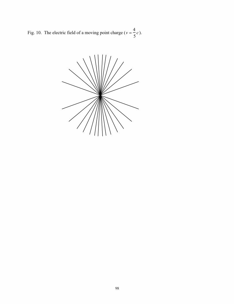
98

Fig. 10. The electric field of a moving point charge (v =45

c ).

99

Fig. 11. The electric field lines of a right-handed circularly polarized photon orbitsphere as seen along the axis of propagation in the lab inertial reference frame as it passes a fixed point.

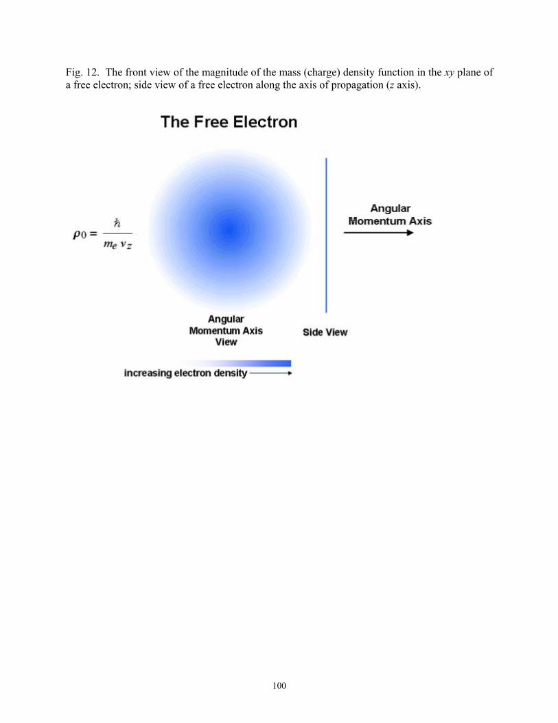
100

Fig. 12. The front view of the magnitude of the mass (charge) density function in the xy plane of a free electron; side view of a free electron along the axis of propagation (z axis).

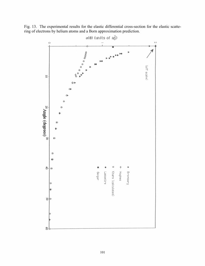
101

Fig. 13. The experimental results for the elastic differential cross-section for the elastic scatte-ring of electrons by helium atoms and a Born approximation prediction.

102

Fig. 14. The closed form function (Eqs. (139) and (140)) for the elastic differential cross section for the elastic scattering of electrons by helium atoms. The scattering amplitude function, F(s) (Eq. (138), is shown as an insert.

103

Fig. 15. The radius of the universe as a function of time.

104

Fig. 16. The expansion/contraction rate of the universe as a function of time.

105

Fig. 17. The Hubble constant of the universe as a function of time.

106

Fig. 18. The density of the universe as a function of time.

107

Fig. 19. The power of the universe as a function of time.

108

Fig. 20. The temperature of the universe as a function of time during the expansion phase.

109

Fig. 21. The differential expansion of the light sphere due to the acceleration of the expansion of the cosmos as a function of time.

110

Fig. 22. Step One. Each point or coordinate position on the continuous two-dimensional elec-tron orbitsphere defines an infinitesimal charge (mass)-density element which moves along a geodesic orbit comprising a great circle. Two such infinitesimal charges (masses) at points 1 (moving counterclockwise on the great circle in the y'z' plane) and 2 (moving clockwise on the great circle in the x'z' plane) of two orthogonal great circle current loops in the basis frame are considered as sub-basis elements to generate the current density corresponding to the spin quan-

tum number, s =12

; ms = ±12

. The xyz-system is the laboratory frame, and the orthogonal-

current-loop basis set is rigid with respect to the x'y'z' system that undergoes transformations to generate the elements of the electron current density function. The angular momentum of the

orthogonal great circle current loops in the x'y' plane is 2 2

.

111

Fig. 23. Step Two. The orthogonal great circle basis set is rotated ∆α x' =π2

with respect to the basis

set of Step One shown in Figure 22, and the direction of the current of the loop in the y'z' plane is re-versed. Point 1 now moves clockwise on the great circle in the y'z' plane, and point 2 moves counter clockwise on the great circle in the x'y' plane. The angular momentum of the orthogonal great circle

current loops in the –xz plane is 2 2

, corresponding to each of the z and –x components of magnitude

4.

112

Fig. 24. The trajectory of the resultant angular momentum vector of the orthogonal great circle

current loops of magnitude 2 2

during Step One.

start at

end at

-y

x

z

θ

4,−

4, 0

⎛ ⎝

⎞ ⎠

−4

,4

, 0⎛ ⎝

⎞ ⎠

2 2

113

Fig. 25. The angular momentum components of the orbitsphere and S in the rotating coordinate system XR , YR , and ZR that precesses at the Larmor frequency about ZR such that the vectors are stationary.

XR

YR

ZR

θ =

π3

S

43

4

2

2

114

Fig. 26. The angular momentum components of the orbitsphere and S in the stationary coordi-nate system. S and the components in the xy plane precesses at the Larmor frequency about the z axis.

S

x

y

z

43

42

2

115

Fig. 27. Coordinate system of crossed electric field E y , corresponding to the Hall voltage, ma-gnetic flux B x , due to applied field, and superconducting current iz .

y

x

i

B

Ez

116

Fig. 28. Coordinate system of crossed electric field E r , corresponding to the Hall voltage, ma-gnetic flux Bθ , due to applied field, and superconducting current iφ .

Bθ Er

iφ

Bθ Er

iφ