Embed Size (px)
DESCRIPTION
The fundamentals of soil mechanics.
Citation preview

10/9/2008
1
Golder Geomechanics Centre
CIVL2210 Fundamentals of Soil Mechanics
Professor David WilliamsDr Dorival Pedroso
ngth
Com
pres
sibi
lity
Perm
eabi
lity
Topics
Soil classificationSoil phase (solids/water/air) relationshipsPrinciple of effective stressPore water pressureSeepage through soilsSoil strength testing and theoriesSoil consolidation testing and settlement theories
Stre
n Soil consolidation testing and settlement theoriesFailure conditions in soilsClay mineralogy
ngth
Com
pres
sibi
lity
Perm
eabi
lity
Lecture/Tutorial/Practical Schedule
Week Lectures Tutorials Practicals
1 L1: Introductory slide showL1: Soil classification
L2: Soil phase relationships
2 L3: Principle of effective stressL4: Pore water pressure
T1: Definitions and classification
P1: Visual classification &P2:Atterberg limits3 L5: Seepage through soils T2: Pore pressure &
effective stress
4 L5: Seepage through soils T3: Darcy’s Law
Stre
n 5: Seepage t oug so s 3: a cy s aw
5 L5: Seepage through soils T4: Seepage
6 L6: Strength testing and theories T4: Seepage P3: Laboratory compaction &P4: Field density and CBR
7 L6: Strength testing and theories T5: Shear strength
8 L7: Strength testing and theories T5: Shear strength
9 L7: Consolidation testing andtheories
T6: Consolidation
10 L7: Consolidation testing andtheories
T6: Consolidation P5: Unconfined compression &P6: Consolidation
ngth
Com
pres
sibi
lity
Perm
eabi
lity
Lecture/Tutorial/Practical Schedule
Week Lectures Tutorials Practicals
MID-SEMESTER BREAK
11 L8: Failure conditions in soil masses
Practice Exam P5: Unconfinedcompression and vane shear &P6: Consolidation
12 L9: Clay mineralogy T7: Lateral earthpressures
13 Revision Revision
EXAMINATION PERIOD
Stre
n EXAMINATION PERIOD
ngth
Com
pres
sibi
lity
Perm
eabi
lity
Schedule
LECTURESFrom 10:00 to 11:50 am on Tuesdays in 63-348
TUTORIALSFrom 2:00 to 3:50 pm on Thursdays in 42-216
PRACTICALS
Stre
n
From 2:00 to 4:00 pm on Mondays, Tuesdays, Wednesdays and Fridays in 48C-SOILS LAB
ASSESSMENTEnd of semester (multiple choice) exam:Tutorials:Completion of Practicals:
65%20%15%
ngth
Com
pres
sibi
lity
Perm
eabi
lity
1 Soil Classification
1.1 Particle Size Distribution AnalysisParticle size limits:
Boulders > 200 mm
Cobbles 60-200 mm
Gravel 2-60 mmCoarse-grained
Stre
n
Obtain distribution of sand size and coarser by sievingObtain distribution of silt and clay size by sedimentation (hydrometer), or laser
Sand 0.06-2 mm
Silt 0.002-0.06 mm
Clay < 0.002 mm
Fine-grained(can’t see or feel particles)
g

10/9/2008
2
ngth
Com
pres
sibi
lity
Perm
eabi
lity
1 Soil Classification (cont.)
1.2 Atterberg LimitsOf material passing 0.425 mm
SOILVOLUME
Stre
n
Shrinkage limit, SL:
Plastic limit, PL:Liquid limit, LL:Plasticity index:
SL PL LLMOISTURE CONTENT, w
Solid Semi-solid Plastic Liquid
w at which soil reaches its minimum volumeon air drying from LL
minimum w at which soils deforms plastically
minimum w at which soil flowsPLLLI P −=
ngth
Com
pres
sibi
lity
Perm
eabi
lity
1 Soil Classification (cont.)
1.2 Atterberg Limits (cont.)
Liquidity index,
Activity,
PL I
PLwI −=
massby clay %PIA =
Stre
n
Emerson Class Number of a soil to assess slakability and dispersion – particularly relevant to the weathering of mine wastes on exposure
1 Low activity 1 2 Intermed. activity
4 High activity
<⎧⎪= −⎨⎪>⎩
ngth
Com
pres
sibi
lity
Perm
eabi
lity
1 Soil Classification (cont.)
Immerse air-dried 2 mm to 4 mm dia. crumbs of soil in distilled water in a beaker
Slaking
Complete dispersion Class 1 Some dispersion Class 2 No dispersion
I i t d ld d 3 di t il b ll i di till d t i b k
No slaking
Swelling Class 7 No swelling Class 8
Stre
n Immerse moistened remoulded 3 mm diameter soil balls in distilled water in a beaker
Dispersion Class 3 No dispersion
No calcite or gypsum present
Make up 1:5 soil/water suspension in a test tube and shake
Dispersion Class 5 Flocculation Class 6
Calcite or gypsum present Class 4
Determination of Emerson class number of a soil
ngth
Com
pres
sibi
lity
Perm
eabi
lity
1 Soil Classification (cont.)
1.3 Unified Soil ClassificationA common notation for describing soils, from which engineering properties, behaviour and use can be inferred (Lambe and Whitman, 1979):
Main SoilTypes Prefix
Coarse-grained soils ( < 50 % passing 0.06 mm)
Stre
n
GRAVEL predominant G
SAND predominant S
Fine-grained soils ( > 50 % passing 0.06 mm)
Inorganic CLAY Above A-line C
SILTBelow A-line
M
ORGANIC SOILS O
Fibrous soils
PEAT (no suffix) Pt
ngth
Com
pres
sibi
lity
Perm
eabi
lity
1 Soil Classification (cont.)
Sub-division Suffix
Coarse-grained soils with < 5 % passing 0.06 mm
Well-graded (spread of sizes) W
Poorly-graded (uniform or gap-graded) P
Coarse-grained soils with > 12 % passing 0.06 mm
Stre
n
Clay fines Above A-line C
Silt fines Below A-line M
Fine-grained soils
Low plasticity LL < 50 % L
High plasticity LL > 50 % H
ngth
Com
pres
sibi
lity
Perm
eabi
lity
1 Soil Classification (cont.)
Stre
n

10/9/2008
3
ngth
Com
pres
sibi
lity
Perm
eabi
lity
1 Soil Classification (cont.)
y In
dex
40
50
6
0
Dry strength and stickinessIncrease with increasingPlasticity Index, and dilatancy(permeability) decreases.
CHLow plasticity
High plasticity
Stre
n
Liquid Limit
Plas
ticity
0 10 20 30 40 50 60 70 80 90 100
0
10
20
30
CL
OHorMH
OLorML
CL
MLCL-ML
ngth
Com
pres
sibi
lity
Perm
eabi
lity
1 Soil Classification (cont.)
1.4 Engineering Use ChartBased on Unified Soil ClassificationRelates engineering parameters (strength, compressibility and permeability when compacted, and workability) applied to dams, canals, foundations and roads1 = highly desirable, 14 = highly undesirable(Lambe and Whitman, 1979)
Stre
n
ngth
Com
pres
sibi
lity
Perm
eabi
lity
1 Soil Classification (cont.)
Stre
n ngth
Com
pres
sibi
lity
Perm
eabi
lity
1 Soil Classification (cont.)
1.5 Other Classification SystemsOther classification systems include those directed towards specific applications, such as road design and agriculture (Fang, 1990)There are classification systems based on specific engineering properties, such as strength (for clays) or relative density (for sands)
Stre
n
ngth
Com
pres
sibi
lity
Perm
eabi
lity
2 Phase (solids/water/air) Relationships
UnitsVoid ratio: -
VOLUMES WEIGHTSPROPORTIONS BY
VOLUME WEIGHT
VVeV
=
e
1w1
AV
WV
SV SWWW
0 Air
Water
Solids
AV
Stre
n
Porosity: -
Relative density: -
Moisture content: %
Degree of saturation: %
SV
1V
T
V enV e
= =+
max
max minR
e eDe e
−=
−
100W
S
WwW
= ⋅
100W
A W
VSV V
= ⋅+
ngth
Com
pres
sibi
lity
Perm
eabi
lity
2 Phase (solids/water/air) Relationships (cont.)
Measurable? Typical valuesVoid ratio: No 3 (slurry) to 0.33
VOLUMES WEIGHTSPROPORTIONS BY
VOLUME WEIGHT
VVeV
=
e
1w1
AV
WV
SV SWWW
0 Air
Water
Solids
VV
void
s
Stre
n
( y)
Porosity: No 0.75 (slurry) to 0.33
Relative density: Yes 30 to 65%
Moisture content: Yes 100 to 5%
Degree of saturation: No 0 (dry) to 100%
SV
1V
T
V enV e
= =+
max
max minR
e eDe e
−=
−
100W
S
WwW
= ⋅
100W
A W
VSV V
= ⋅+

10/9/2008
4
ngth
Com
pres
sibi
lity
Perm
eabi
lity
2 Phase (solids/water/air) Relationships (cont.)
UnitsTotal unit weight: kN/m3
Unit weight of water: kN/m3
TT
T
WV
γ =
9.81Wγ =
11 W
w Ge
γ+= ⋅ ⋅
+
Stre
n
Effective unit weight: kN/m3
Dry unit weight: kN/m3
Specific gravity: -
' T Wγ γ γ= −
SD
T
WV
γ =
S
S W
WGV γ
=⋅
1 1T
WG
w eγ γ= = ⋅+ +
G w S e⋅ = ⋅
ngth
Com
pres
sibi
lity
Perm
eabi
lity
2 Phase (solids/water/air) Relationships (cont.)
Measurable? Typical valuesTotal unit weight: Yes (if regular) 15 to 20 kN/m3
Unit weight of water: kN/m3 Yes 9.81 kN/m3
TT
T
WV
γ =
9.81Wγ =
11 W
w Ge
γ+= ⋅ ⋅
+
Stre
n
Effective unit weight: Yes 5 to 10 kN/m3
Dry unit weight: Yes (if regular) 0.5 to 20 kN/m3
Specific gravity: Yes 1.3 (coal) to 2.7to 19.3 (gold)
' T Wγ γ γ= −
SD
T
WV
γ =
S
S W
WGV γ
=⋅
1 1T
WG
w eγ γ= = ⋅+ +
G w S e⋅ = ⋅
ngth
Com
pres
sibi
lity
Perm
eabi
lity
3 Principle of Effective Stress
3.1 Force, pressure, and stress (review)
=p FA
-F FA
pAiA
ExternalforceInternal
pressure
→=σ
dA 0lim dF
dA
Internalstress
Observedarea
Stre
n
Pressure and stressdepend on Area
Pressure and stress vary on Space
There are at least x and ycomponents of stress (in 2D)
pAii
A
A σAx
σAy = 0
dA ngth
Com
pres
sibi
lity
Perm
eabi
lity
3 Principle of Effective Stress (cont.)
3.1 Force, pressure, and stress (cont.)
Pressure and stress are better related with material mechanical changes (damage, failure, stretching, …) than forces
F F=
Stre
n
A
σ V
Ground =AV
A
p FA
AA
=BV
B
p FA
AB
<<
σ H
ngth
Com
pres
sibi
lity
Perm
eabi
lity
3 Principle of Effective Stress
σwu
Stre
n
wσ σ' = - u
Grains
Water
Air
σ' ngth
Com
pres
sibi
lity
Perm
eabi
lity
3 Principle of Effective Stress (cont.)
wσ σ' = - u
σ
Stre
n
Analogy
σwu
σ'

10/9/2008
5
ngth
Com
pres
sibi
lity
Perm
eabi
lity
3 Principle of Effective Stress (cont.)Hydromechanicalanalogy for load-sharing and consolidationa) Physical exampleb) Hydromechanical
analogc) Load applied
with valve closedd) Piston moves as
Stre
n
)water escapes
e) Equilibrium with no further flow
f) Gradual transfer of load
ngth
Com
pres
sibi
lity
Perm
eabi
lity
3 Principle of Effective Stress (cont.)
Effective stress σ’ is taken by the soil skeleton
In a water-saturated soil:where σ is the total stress (weight of everything above a particular point, including water), uw is the pore water pressure
' = −σ σ wu
σwu
σ'
Stre
n
In a dry soil:
Changes in σ’ lead to deformations and changes in strength – the soil grains and pore water are assumed to be incompressible
In a water-saturated soil, deformation on the application of stress is directly related to the expulsion of pore water. Thus, related to permeability (coupled phenomena)
' =σ σσ
σ'
ngth
Com
pres
sibi
lity
Perm
eabi
lity
The total vertical stress σV at a given depth in the soil profile is equal to the weight of everything above that point, including the wet soil and any surface water or surface loading
4 Geostatic Stresses
water table
γ T
ground
a
σV
at A
=σ γVA T a?=σ HA
Stre
n
γ SAT
b
A
c
depth z
at B
at C
at A
C
= + γσ σVC VA SAT c?=σ HC
= + γσ σVB VA SAT b?=σ HB
?σ HA
B
ngth
Com
pres
sibi
lity
Perm
eabi
lity
3 Principle of Effective Stress (cont.)
Sand shear strength is proportional to σ’:where is the angle of internal friction of the sand.
Clay shear strength is given by:
is also proportional to σ’, the constant of proportionality dependent on the over-consolidation ratio (OCR):
' tanτ σ φ= ⋅
or 'uc cτ =
τ
φτ
τ
Stre
n
( )
where NC is normally consolidated, OC is overconsolidated, and m is a power, found experimentally to have a value of about 0.8:
constant (typically 0.25)' NC
τσ
⎛ ⎞ = ≈⎜ ⎟⎝ ⎠
( )' '
m
OC NC
OCRτ τσ σ
⎛ ⎞ ⎛ ⎞≈ ⋅⎜ ⎟ ⎜ ⎟⎝ ⎠ ⎝ ⎠
ngth
Com
pres
sibi
lity
Perm
eabi
lity
3 Principle of Effective Stress (cont.)
In soils of high permeability (sands and gravels), any excess u induced by an applied stress generally dissipates instantaneously, with the applied stress (σ) transferring instantaneously to the soil skeleton (σ’) → DRAINED BEHAVIOUR
Quick conditions or liquefaction are an exception. Here the rate of stress application is more rapid than the rate of drainage possible, σ’ ≤ 0, and seepage stresses exceed the strength of the soil
Stre
n seepage stresses exceed the strength of the soil
In saturated soils of low permeability (clays), any applied stress is initially taken as excess u. This dissipates with time and the water (excess u) to the soil skeleton (σ’) → UNDRAINED SHORT TERM AND DRAINED LONG TERM BEHAVIOUR. Refer to water-bed analogy (Lambe and Withman, 1979)
ngth
Com
pres
sibi
lity
Perm
eabi
lity
4 Pore Water Pressure
4.1 Hydrostatic Pore Water PressureHydrostatic pore water pressure increases in proportion to the depth below the water table:
PORE WATER PRESSURE, u
Water table
Stre
n
DEPTH, z
W Wu zγ= ⋅

10/9/2008
6
ngth
Com
pres
sibi
lity
Perm
eabi
lity
Hydrostatic pore water pressure uw increases in proportion to the depthz below the water table: (γw = 9.81 kN.m3)
4 Geostatic Stresses (cont.)
water table
ground
uw
0=WAu
= ⋅γ WW Wu z
? at A
Unsaturatedsoil mechanics
Assumption
Stre
n
b
c
depth z
at B
at CC
= γ WWCu c
B
= γWWBu b
Aat A ng
thC
ompr
essi
bilit
yPe
rmea
bilit
y
The effective vertical stress σ’V at a given depth in the soil profile is the difference between total stress and water pressure
4 Geostatic Stresses (cont.)
water table
ground
= −σ σ V WA AV A' u
0K≈σ σHA VA' '
σV’
at A
Stre
n A 0Kσ σHA VA
depth z
at B
at C
at A
B
= −σ σ V WB BV B' u
0K≈σ σHB VB' '
C
= −σ σ V WC CV C' u
0K≈σ σHC VC' '
ngth
Com
pres
sibi
lity
Perm
eabi
lity
4 Geostatic Stresses (cont.)
Summary:1) The total vertical stress σV at a given depth in the soil profile is equal to the weight of everything above that point, including the wet soil and any surface water or surface loading.
2) The total vertical stress σV due to wet soil is equal to its total unit weight multiplied by the depth of soil above that point at that total unit weight
Stre
n weight.
3) The hydrostatic pore water pressure uW at a given depth in the soil profile is equal to the height of the water table above that point multiplied by the unit weight of water (9.81 kN.m3).
4) The effective vertical stress σ’V at a given depth in the soil profile is the difference between total stress and water pressure
= ⋅σ γV T z
= −σσ V V W' u = ⋅σ σ0H VK' '
ngth
Com
pres
sibi
lity
Perm
eabi
lity
4 Pore Water Pressure (cont.)
4.2 Pore water suctionPore water suction can occur in two forms:
matric (or capillary) and;solute (or osmotic)
Matric suction is readily incorporated within the effective stress principle, and changes in matric suction will give rise to deformation and changes in shear strength. By definition, matrix suction is zero at and below the water table and increases above the water table
Stre
n and below the water table, and increases above the water tableThe magnitude of matric suction is a function of the soil pore size. Sands are only capable of maintaining about 1 m height of capillary rise above the water table. In clays, very high matrix suctions can develop above the water table towards the ground surface. Silts are intermediate between these extremes
ngth
Com
pres
sibi
lity
Perm
eabi
lity
4 Pore Water Pressure (cont.)4.2 Pore water suction (cont.)
PORE WATER PRESSURE, uNet evaporation Net percolation
CLAY
SILT
SAND
Water table~1 m
Stre
n
The magnitude of solute suction is a function of the total dissolved salt concentration of the pore water. It can occur both above and below the water table, and in an arid climate may well be of the order of 100 to 100 kPa for an expansive clay profile.
DEPTH, z
Hydrostatic (No flow)
W Wu zγ= ⋅
ngth
Com
pres
sibi
lity
Perm
eabi
lity
4 Pore Water Pressure (cont.)
4.2 Pore Water Suction (cont.)
Changes in solute suction may give rise to deformation and changes in shear strength. However, a change in solute suction would require a dissolved salt differential to drive it, the solute suction would change only slowly, and it is unlikely that the driving dissolved salt differential would be maintained for a sufficiently long time. It is therefore common practice to ignore solute suction-induced deformation and
Stre
n common practice to ignore solute suction induced deformation and changes in shear strength.
Pore water suction is generally expressed in terms of pF units (a logarithmic scale in which pF 3 ≈ 100 kPa pressure, pF 4 ≈ 1,000 kPa, and pF 5 ≈ 10,000 kPa. In the seasonal suction profiles, the lower bound line may be essentially solute suction, with the difference between the two lines representing the seasonal variation of matrix suction (Cameron and Walsh, 1984).
10/9/2008
7
ngth
Com
pres
sibi
lity
Perm
eabi
lity
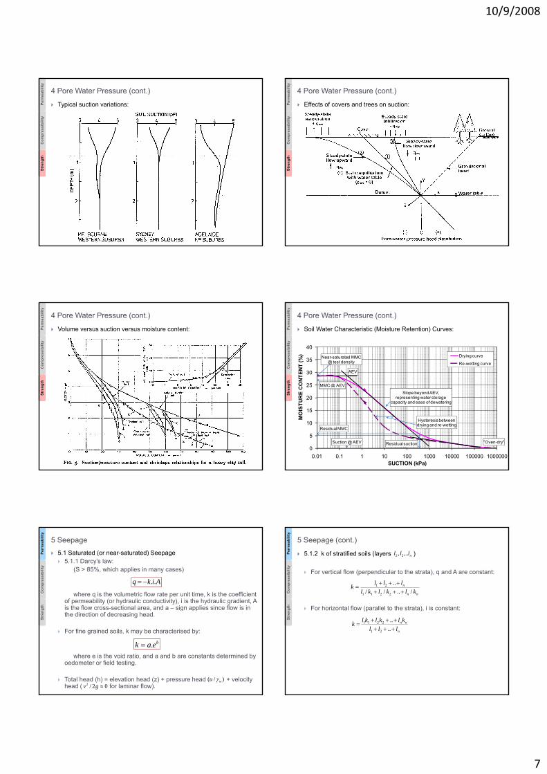
4 Pore Water Pressure (cont.)
Typical suction variations:
Stre
n ngth
Com
pres
sibi
lity
Perm
eabi
lity
4 Pore Water Pressure (cont.)
Effects of covers and trees on suction:
Stre
n
ngth
Com
pres
sibi
lity
Perm
eabi
lity
4 Pore Water Pressure (cont.)
Volume versus suction versus moisture content:
Stre
n ngth
Com
pres
sibi
lity
Perm
eabi
lity
4 Pore Water Pressure (cont.)
Soil Water Characteristic (Moisture Retention) Curves:
25
30
35
40
CO
NTE
NT
(%) Drying curve
Re-wetting curve
MMC @ AEV
AEV
Near-saturated MMC@ test density
Stre
n
0
5
10
15
20
25
0.01 0.1 1 10 100 1000 10000 100000 1000000
MIN
ING
MO
ISTU
RE
C
SUCTION (kPa)
MMC @ AEV
Residual suction
Slope beyond AEV,representing water storage
capacity and ease of dewatering
"Oven-dry"
Hysteresis betweendrying and re-wetting
Suction @ AEV
Residual MMC
ngth
Com
pres
sibi
lity
Perm
eabi
lity
5 Seepage5.1 Saturated (or near-saturated) Seepage
5.1.1 Darcy’s law:(S > 85%, which applies in many cases)
where q is the volumetric flow rate per unit time, k is the coefficient of permeability (or hydraulic conductivity), i is the hydraulic gradient, A is the flow cross-sectional area, and a – sign applies since flow is in
Aikq ..−=
Stre
n
gthe direction of decreasing head.
For fine grained soils, k may be characterised by:
where e is the void ratio, and a and b are constants determined by oedometer or field testing.
Total head (h) = elevation head (z) + pressure head + velocity head ( for laminar flow).
beak .=
)/( wu γ02/2 ≈gv
ngth
Com
pres
sibi
lity
Perm
eabi
lity
5 Seepage (cont.)
5.1.2 k of stratified soils (layers )
For vertical flow (perpendicular to the strata), q and A are constant:
For horizontal flow (parallel to the strata), i is constant:
nlll ,.., 22
nn
n
klklkllllk
/..//..
2211
21
++++++
=
Stre
n (p ),
n
nn
lllklklklk
++++++
=....
21
2211

10/9/2008
8
ngth
Com
pres
sibi
lity
Perm
eabi
lity
5 Seepage (cont.)5.2 Laboratory Permeability Testing
5.2.1 Saturated permeability testingFor m/s (clean sands and gravels), use a constant head permeameter.
For m/s (silts and clays), use a falling head permeameter.
410 −>k
47 1010 −− << k
Stre
n
For m/s (clays), use indirect methods such as an oedometer test.
Typical values of (Fang, 1990)
Partially saturated is difficult to determine directly, since its attempted measurement changes the degree of saturation. It may be estimated indirectly via the suction/moisture content characteristic of the soil, together with theory.
k
k
710 −<k
ngth
Com
pres
sibi
lity
Perm
eabi
lity
5 Seepage (cont.)
5.2.1 Saturated permeability tests (cont.)
Stre
n
ngth
Com
pres
sibi
lity
Perm
eabi
lity
5 Seepage (cont.)
5.2.2 Constant head permeameter (Head, 1982):
Stre
n ngth
Com
pres
sibi
lity
Perm
eabi
lity
5 Seepage (cont.)
5.2.3 Falling head permeameter (Head, 1982):
Stre
n
ngth
Com
pres
sibi
lity
Perm
eabi
lity
5 Seepage (cont.)
5.2.4 Indirect determination of k
For low permeability soils, k may be determined indirectly from the results of oedometer or Rowe consolidometer tests:
wvv mck γ..=
Stre
n ngth
Com
pres
sibi
lity
Perm
eabi
lity
5 Seepage (cont.)
5.3 Field Measurement of PermeabilityFor coarse grained soils and fractured rock use pumping tests.
Unconfined flow (Cedergren, 1977):
1 22 2
2 1
l n ( / )q r rkh hπ
⎛ ⎞= ⋅ ⎜ ⎟−⎝ ⎠
( r2 / r1 )
Stre
n

10/9/2008
9
ngth
Com
pres
sibi
lity
Perm
eabi
lity
5 Seepage (cont.)
5.3 Field Measurement of Permeability (cont.)
Confined flow:
where q is the volumetric flow rate pumped from the well, and are the radii from the well to the observation boreholes 1 and 2, and are the total heads at the observation boreholes 1 and 2,
d D i h hi k f h fi d if
⎟⎟⎠
⎞⎜⎜⎝
⎛−
⋅=12
21 )/ln(2 hh
rrD
qkπ
1r2r
1h 2h
Stre
n and D is the thickness of the confined aquifer.
For fine grained soils use a constant head test (infer k from the volume of water required to maintain the head constant for a given geometry), or a falling head test (infer k from the rate of fall of an elevated head in a small diameter standpipe).
ngth
Com
pres
sibi
lity
Perm
eabi
lity
5 Seepage (cont.)
5.4 Seepage Flow5.4.1 1-D flow
For upward vertical flow in sands, the quick condition is given by:
5.4.2 2-D flowAssuming homogeneous and isotropic conditions within the
0'≤vσ
1≈−=
w
wsaturatedcriticali
γγγ
Stre
n seepage zone, and both the soil particles and pore water to be incompressible, the CONTINUITY EQUATION is given by:
where and are the apparent (not actual) velocities in x (horizontal) and z (vertical) directions, respectively.In terms of total head h, the LAPLACE EQUATION is given by:
0=∂∂
+∂∂
zv
xv zx
0=∂∂
+∂∂
zh
xh
xv zv
ngth
Com
pres
sibi
lity
Perm
eabi
lity
5 Seepage (cont.)
5.4.2 2-D flow (cont.)The Laplace Equation may be solved by:
Graphical means using FLOW NETELECTRICAL ANALOGUE: the flow of water through soil, driven by a head differential, being analogous to the flow of electrical current through a conducting medium, driven by a voltage differential.NUMERICAL TECHNIQUES:
Stre
n NUMERICAL TECHNIQUES:For anisotropic conditions, the STEADY STATE SEEPAGE EQUATION is given by:
where and are the total heads in the x and z directions, respectively, and and are the coefficients of permeability in the x and z directions, respectively.
0=∂∂⋅+
∂∂⋅
zhk
xhk z
zx
x
xh zhxk zk
ngth
Com
pres
sibi
lity
Perm
eabi
lity
5 Seepage (cont.)
5.5 Flow Nets – RulesSets of flow lines (average trajectories of seepage) and equipotentiallines (loci of constant total head) may be drawn within a seepage zone to form a FLOW NET of curvilinear squares.A permeable boundary is an equipotential line.An impermeable boundary is a flow line.Equipotential lines intersect a line of constant u (often u=0) at equal drops in head:
Stre
n drops in head:If the line of constant u is a phreatic line (and hence a flow line), equipotentials will intersect it at right angles.If the line of constant u is a drain (and hence not a line flow), intersections will not necessarily be at right angles.
Examples of flow net construction (Cedergren, 1997).
ngth
Com
pres
sibi
lity
Perm
eabi
lity
5 Seepage (cont.)
5.5 Flow Nets (cont.)
Stre
n ngth
Com
pres
sibi
lity
Perm
eabi
lity
5 Seepage (cont.)
5.5 Flow Nets (cont.)
Stre
n

10/9/2008
10
ngth
Com
pres
sibi
lity
Perm
eabi
lity
5 Seepage (cont.)
5.5 Flow Nets (cont.)
Stre
n ngth
Com
pres
sibi
lity
Perm
eabi
lity
5 Seepage (cont.)
5.5 Flow Nets (cont.)
Stre
n
ngth
Com
pres
sibi
lity
Perm
eabi
lity
5 Seepage (cont.)
5.5 Flow Nets (cont.)
Stre
n ngth
Com
pres
sibi
lity
Perm
eabi
lity
5 Seepage (cont.)
5.5 Flow Nets (cont.)
Stre
n
ngth
Com
pres
sibi
lity
Perm
eabi
lity
5 Seepage (cont.)5.5 Flow Nets (cont.)
The flow through the seepage zone is given by:
where is the drop in total head across the seepage zone, M/N is the flow net shape factor, M is the number of flow tubes and N is the number of equipotential drops within the seepage zone.The velocity of flow varies throughout the seepage zone, the apparent velocity increasing as the dimension of the flow net decreases.Th ithi th d f th t t th id f th
NMhkq ⋅Δ⋅=
hΔ
Stre
n The u within the seepage zone reduces from that at the side of the seepage zone with the highest total head, according to the number of equipotential drops to the point in question ( and rises from that at the other side).Flow lines (and equipotential lines) are refracted on crossing an interface between isotropic soils of different k:
where and are the widths of the flow tubes in materials of and , respectively (refer to examples from Cedergren, 1977).
1w 2w 1k2k
2
1
2
1
kk
ww
=
ngth
Com
pres
sibi
lity
Perm
eabi
lity
5 Seepage (cont.)
5.5 Flow Nets (cont.)
Stre
n

10/9/2008
11
ngth
Com
pres
sibi
lity
Perm
eabi
lity
5 Seepage (cont.)
5.5 Flow Nets (cont.)
Stre
n ngth
Com
pres
sibi
lity
Perm
eabi
lity
5 Seepage (cont.)
5.5 Flow Nets (cont.)
Stre
n
ngth
Com
pres
sibi
lity
Perm
eabi
lity
5 Seepage (cont.)
5.5 Flow Nets (cont.)
Stre
n
For anisotropic soils, flow nets may be used with a transformed scale (refer to examples from Cedergren, 1977):
and xkkx
x
z ⋅=' xzkkNMhq ⋅⋅Δ=
ngth
Com
pres
sibi
lity
Perm
eabi
lity
5 Seepage (cont.)
5.5 Flow Nets (cont.)
Stre
n
ngth
Com
pres
sibi
lity
Perm
eabi
lity
5 Seepage (cont.)
5.5 Flow Nets (cont.)
Stre
n ngth
Com
pres
sibi
lity
Perm
eabi
lity
5 Seepage (cont.)
5.6 Special Cases5.6.1 Local effects of seepage stresses
Quick conditions can occur in sands if seepage stresses render
This can be avoided by decreasing i (increase l using a cut-off and/or decrease h by dewatering) and/or by increasing by surcharging.
0' ≤vσ
'vσ
Stre
n Seepage stresses can cause have in clays, and, in the extreme may facilitate piping.
5.6.2 Flow through discontinuous rockThe permeability of discontinuous rock depends on the spacing, persistence, aperture, and filling of the joints, and on the stresses applied across the joints.Limestone and other water-soluble rocks can develop solution channels which enlarge with time, increasing seepage rates.

10/9/2008
12
ngth
Com
pres
sibi
lity
Perm
eabi
lity
5 Seepage (cont.)
5.7 Unsaturated Seepage5.7.1 Partially saturated permeability
The water permeability of soils decreases dramatically (by up to several orders of magnitude) as it desaturates, desaturation causing pore water to retreat into ever tighter menisci at the particle contacts. The menisci are associated with the development of soil suction, providing the basis for estimating partially saturated permeability from the suction/moisture content characteristic of the
Stre
n permeability from the suction/moisture content characteristic of the soil, together with theory.The air permeability of soils increases even more dramatically as it desaturates.Fredlund and Rahardjo (1993) reproduced coefficients of air and water permeability versus gravimetric moisture content.
ngth
Com
pres
sibi
lity
Perm
eabi
lity
5 Seepage (cont.)
5.7 Unsaturated Seepage (cont.)5.7.1 Partially saturated permeability (cont.)
Stre
n
ngth
Com
pres
sibi
lity
Perm
eabi
lity
5 Seepage (cont.)
5.7.2 Suction/Moisture Content Characteristic:Different suction/moisture content characteristics are obtained, depending on the path followed, and the disturbance to the structure of the soil.This is demonstrated by data for London (heavy) clay obtained by Croney and Coleman (1954), which has a liquid limit of 77%, plastic limit of 27% and plasticity index of 50%.
Curve A was obtained by drying the undisturbed clay from its
Stre
n Curve A was obtained by drying the undisturbed clay from its natural moisture content (pF close to 0). The undisturbed clay remains saturated to a moisture content of 22% (pF of about 4). Further reduction in moisture content (increase in pF) is accompanied by little reduction in volume (as water is replaced by air in the pores)Curve B was obtained by subsequent wetting up of the clay, and demonstrates some irreversible structural change on oven-drying. Re-drying follows curve C. Subsequent wetting and drying cycles follow curves B and C.
ngth
Com
pres
sibi
lity
Perm
eabi
lity
5 Seepage (cont.)
5.7.2 Suction/Moisture Content Characteristic (cont.)Curve D was obtained by slurrying the clay at a high moisture content, partially destroying the structure of the clay, then drying it from pF 0 to pF 7 (oven dry).Curves B and D represent the limiting cases.Curves A and D coincide above pF 4.8.Curves E and F show that cycling below pF 4.8 results in a series of loops different for each maximum suction
Stre
n of loops different for each maximum suction.Curve G is unique to the clay, representing the critical state obtained for the clay on disturbance at any moisture content or suction. Both the liquid and plastic limits lie on curve G.
ngth
Com
pres
sibi
lity
Perm
eabi
lity
5 Seepage (cont.)
5.7.2 Suction/Moisture Content Characteristic (cont.)
Stre
n ngth
Com
pres
sibi
lity
Perm
eabi
lity
4 Pore Water Pressure (cont.)
Soil Water Characteristic (Moisture Retention) Curves:
25
30
35
40
CO
NTE
NT
(%) Drying curve
Re-wetting curve
MMC @ AEV
AEV
Near-saturated MMC@ test density
Stre
n
0
5
10
15
20
25
0.01 0.1 1 10 100 1000 10000 100000 1000000
MIN
ING
MO
ISTU
RE
C
SUCTION (kPa)
MMC @ AEV
Residual suction
Slope beyond AEV,representing water storage
capacity and ease of dewatering
"Oven-dry"
Hysteresis betweendrying and re-wetting
Suction @ AEV
Residual MMC

10/9/2008
13
ngth
Com
pres
sibi
lity
Perm
eabi
lity
5 Seepage (cont.)
5.7.3 Unsaturated seepageSurface evaporation, a surface cover, steady state infiltration, and tress have different effects on the suction profile (Fredlund and Rahardjo, 1993).
Stre
n ngth
Com
pres
sibi
lity
Perm
eabi
lity
5 Seepage (cont.)
5.7.3 Unsaturated seepage (cont.)Unsaturated seepage is highly channelised, but also involves storage. Rather than being bounded by a phreatic line (as in saturated seepage), it is bounded by a wetting-up line, below which the medium is not saturated (for example, unimpeded water flow compared with tailings water flow through a coarse reject bund; the latter seepage rate is about an order of magnitude lower due to the tailings filter cake which forms on the upstream side of the bund, and
Stre
n
this induces unsaturated seepage through the relatively free-draining bund; Williams, 1992).
ngth
Com
pres
sibi
lity
Perm
eabi
lity
6 Strength Testing and Theories
6.1 Strength Testing6.1.1 Direct shear test
The shearbox was designed originally for measuring the friction angle of recompacted sands.The shearbox can also be used to measure the undrained shear strength of clays, but the triaxial test is usually more suitable for this purpose.Consolidated drained tests (for ) and shear reversal tests' 'c φ
Stre
n Consolidated-drained tests (for ), and shear reversal tests (for residual shear strength ) may also be carried out using the shearbox.The soil is placed in a rigid metal box, square in plan (60,100, or 300 mm in dimension), consisting of two halves.The lower half of the box can slide relative to the upper half when a shear force is applied, while a yoke applies a normal force.The soil is forced to shear at the interface between the two halves of the box. During shearing, the shear stress, and shear and normal displacements are measured (Head, 1982).
, c φ, R Rc φ
ngth
Com
pres
sibi
lity
Perm
eabi
lity
6.1 Strength Testing (cont.)6.1.1 Direct shear test (cont.)
6 Strength Testing and Theories (cont.)
N
F
F appliedforce
surface ofshear
N
F
F
reaction
displacement
movement
Stre
n
start of test during relative displacement
The effect of large shear displacement can be obtained in an ordinary shearbox by reversing the shearbox after initial shearing and reshearing, repeating this a number of times to achieve a steady (residual) shear strength (Head, 1982).
The normal stress may be removed during reversal to avoid destroying the shear plane formed on shearing.
soil specimen surface ofsliding length = breadth = L
ngth
Com
pres
sibi
lity
Perm
eabi
lity
6 Strength Testing and Theories (cont.)
6.1 Strength Testing (cont.)6.1.1 Direct shear test (cont.) N
F
F
Stre
n ngth
Com
pres
sibi
lity
Perm
eabi
lity
6 Strength Testing and Theories (cont.)
6.1 Strength Testing (cont.)6.1.1 Direct shear test (cont.)
The large shearbox is 300mm square, requiring a specimen about 150mm thick, and is suitable for particle sizes up to 37.5mm. Such testing is relevant to the design of embankments or earth dams incorporating gravel fill.
The shearbox can also be used for measuring the angle of friction
N
F
F
Stre
n The shearbox can also be used for measuring the angle of friction developed at the interface between a soil and other materials such as steel, concrete or rock. This is achieved by placing a block of the other material to fill the bottom half of the shearbox and forming the soil in the upper half of the shearbox.
Application of shearbox test:The test is best suited to situations in which slip on a pre-determined shear plane occurs, eg. slope instability.

10/9/2008
14
ngth
Com
pres
sibi
lity
Perm
eabi
lity
6 Strength Testing and Theories (cont.)
6.1 Strength Testing (cont.)6.1.1 Direct shear test (cont.)
Advantages of shearbox test:The test is relatively quick and simple.Sample preparation is easy, particularly for sands.The test can be used to determine residual strength and drained strength parameters.
N
F
F
Stre
n Large particle sizes can readily be tested in a large shearbox.The test can be used to determine the angle of friction between soil and other materials.
ngth
Com
pres
sibi
lity
Perm
eabi
lity
6 Strength Testing and Theories (cont.)
6.1 Strength Testing (cont.)6.1.1 Direct shear test (cont.)
Limitations of shearbox test:The soil is constrained to fail along a pre-determined shear plane.The distribution of stresses in shear zone is not uniform.Principle stresses rotate during shear.
N
F
F
Stre
n Drainage cannot be controlled, except by varying the rate of shear.Pore water pressures cannot be measured.The maximum shear deformation is limited by the travel of the apparatus.The sample contact area decreases during shearing, requiring an area correction, except for purely frictional soils.
ngth
Com
pres
sibi
lity
Perm
eabi
lity
6 Strength Testing and Theories (cont.)
6.1 Strength Testing (cont.)6.1.2 Vane shear test
The four-bladed cruciform vane is pushed into soft cohesive soil and then rotated.
The torque required to rotate the cylinder of soil enclosing the vane is measured, from which the undrained shear strength of the soil is
appliedtorque
D
D
H
Stre
n undrained shear strength of the soil is calculated.
A repeat test immediately after remoulding the soil by rapid rotation of the vane provides a measure of the remoulded strength, and hence sensitivity, of the soil (Head, 1982).
ngth
Com
pres
sibi
lity
Perm
eabi
lity
6 Strength Testing and Theories (cont.)
6.1 Strength Testing (cont.)6.1.2 Vane shear test
appliedtorque
D
resistingtorque
Stre
n
D
H
surface areaDHπ=
H
D
vane blades cylinder of soil rotated by vane
ngth
Com
pres
sibi
lity
Perm
eabi
lity
6 Strength Testing and Theories (cont.)
6.1 Strength Testing (cont.)6.1.2 Vane shear test
Assuming a uniform distribution of stress is mobilised over the cylindrical surface scribed by the vane, and that the stress mobilised over the ends is zero at the centre rising to the same value as that over the cylinder at the edge of the vane, the shear strength may be calculated from the measured torque T using
⎛ ⎞
Us
Stre
n
A vane height to diameter ratio of 2:1 generally applies, which results in more than 90% of the resistance to rotation of the vane coming from the vertical cylindrical surface scribed by the vane. As a result any anisotropy can be ignored in the calculation, with the vane providing an estimate of the shear strength acting on a vertical plane.
2 3
2 6UD H DT sπ
⎛ ⎞⋅= ⋅ ⋅ +⎜ ⎟
⎝ ⎠
ngth
Com
pres
sibi
lity
Perm
eabi
lity
6 Strength Testing and Theories (cont.)
6.1 Strength Testing (cont.)6.1.2 Vane shear test (cont.)
Correlation between the vane shear strength and slope failures has shown that the vane may overestimate the shear strength mobilised in slopes. Bjerrum developed a reduction faction related to the plasticity index of the clay (Craig, 1992). However, this reduction factor was derived for sensitive Scandinavian clays and has been found to not apply to clays in warmer climates.
μ
Stre
n and has been found to not apply to clays in warmer climates.1.2
1.0
0.8
0.6
0.40 20 40 60 80 100 120
Plasticity index
μ

10/9/2008
15
ngth
Com
pres
sibi
lity
Perm
eabi
lity
6 Strength Testing and Theories (cont.)6.1 Strength Testing (cont.)
6.1.3 Triaxial TestTriaxial testing(on cylindrical soil samples) includes:
the unconfined compression testthe triaxial compression testand the triaxial extension test.
In a typical triaxial test the cylindrical soil sample is located within a membrane and mounted in the triaxial cell, housed within a load frame.A i l d ll b li d
membrane
Stre
n Axial and cell pressures may be applied independently.Initially, the estimated average in situ stress is applied isotropicallyThe sample is then sheared by either increasing (compression) or decreasing (extension) to failure, holding constant.During shearing, the stresses and strains are measured.Pore water pressures, volumetric strains, and localised small strains (lateral or axial) may also be measured (Head, 1982).
1 3( )σ σ=
1σ
3σ
1σ
3σ
1σ3σ
ngth
Com
pres
sibi
lity
Perm
eabi
lity 6 Strength Testing and
Theories (cont.)
6.1 Strength Testing (cont.)6.1.3 Triaxial Test (cont.)
Stre
n
ngth
Com
pres
sibi
lity
Perm
eabi
lity 6 Strength Testing and
Theories (cont.)
6.1 Strength Testing6.1.3 Triaxial Test
Triaxial tests may also be carried out in a hydraulic stress path cell, which eliminates the
Stre
n eliminates the need for a load frame, and, being hydraulically driven, is more amenable to automated control (Head, 1982). hydraulic driven:
displacement driven:
ngth
Com
pres
sibi
lity
Perm
eabi
lity
6 Strength Testing and Theories (cont.)
6.1 Strength Testing (cont.)6.1.3 Triaxial Test (cont.)
The unconfined compression test is suitable for determining the undrained strength:
Of soil and rock samples which are capable of being formed as self-supporting cylinders.
1( / 2 )uc σ=
Stre
n Triaxial compression and extension tests may be carried out as follows:
Unconsolidated-undrained shearing (for ).Consolidated-undrained shearing (for ).Consolidated-undrained shearing, with pore water pressure measurement (for ).Consolidated-drained shearing (for ).
0, ≈uuc φ0, ≈cucuc φ
',' φc',' φc
ngth
Com
pres
sibi
lity
Perm
eabi
lity
6 Strength Testing and Theories (cont.)
6.1 Strength Testing (cont.)6.1.3 Triaxial Test (cont.)
Modes of failure in a triaxial compression test include barrelling, shear plane failure, and a combination of these two (Head, 1982).
Stre
n
plastic failure (barrelling) brittle failure (shear plane) intermediate type
ngth
Com
pres
sibi
lity
Perm
eabi
lity
6 Strength Testing and Theories (cont.)
6.1 Strength Testing (cont.)6.1.3 Triaxial Test (cont.)
The triaxial test is generally conducted on saturated samples.It may be necessary to apply a back-pressure to the sample, in combination with a confining pressure to force any air into solution and so saturate the sample prior to testing.
back-pressure of typically 200 kPafi i th b t 10 kP b k
Stre
n confining pressure no more than about 10 kPa < back-pressureSaturation is tested by measuring the B pore pressure parameter. For full saturation, B =1, where
Corrections are required to allow for the membrane, friction losses (on the axial load piston), and change in sample area.
( )[ ] 3313 σσσσ Δ⋅=Δ−Δ+Δ=Δ BABu

10/9/2008
16
ngth
Com
pres
sibi
lity
Perm
eabi
lity
6 Strength Testing and Theories (cont.)6.1 Strength Testing (cont.)
6.1.3 Triaxial Test (cont.)Application of triaxial test:
The test is best suited to situations in which vertical compression and/or extension occur, eg. Building or embankment (beneath centre) loading or basement excavation.
Advantages of triaxial test:Failure is not constrained to a pre-determined surface.Th t i d i t i i l t t b tt t ti f
Stre
n The stresses imposed in a triaxial test are a better representation of the in situ stresses than those applied in the shearbox test.The applied stresses are principle stresses.Drainage conditions can controlled and varied.For intact clays, triaxial strength results obtained from good quality samples agree well with field estimates of strength.
Limitations of triaxial test:Setting up sand samples for triaxial testing is difficult.Triaxial strength results from small size samples give unrealistically high estimates of strength for highly fissured clays.
ngth
Com
pres
sibi
lity
Perm
eabi
lity
6 Strength Testing and Theories (cont.)
6.1 Strength Testing (cont.)6.1.4 Unsaturated strength of clays
Undrained shear strength, Su
Suctioneffect
water table
Stre
n
Depth, z
Self-weighteffect
ngth
Com
pres
sibi
lity
Perm
eabi
lity
6 Strength Testing and Theories (cont.)
6.1 Strength Testing (cont.)6.1.5 Strength testing of rocks
Strength testing methods applied to rocks include:the point load index (tensile) strength testthe direct shear testthe triaxial testand the Hoek cell test (Brown, 1981).
Stre
n
The principles involved are similar to those which apply to the strength testing of soils.
ngth
Com
pres
sibi
lity
Perm
eabi
lity
6.2 Strength Theories6.2.1 Idealized stress/strain behaviour
Elastic
6 Strength Testing and Theories (cont.)
Stre
n
STRAIN
STRESS
ngth
Com
pres
sibi
lity
Perm
eabi
lity
6.2 Strength Theories6.2.1 Idealized stress/strain behaviour
Rigid, perfectly plastic
6 Strength Testing and Theories (cont.)
STRESS
Stre
n
Elastic, perfectly plastic
STRAIN
STRAIN
STRESS
ngth
Com
pres
sibi
lity
Perm
eabi
lity
6.2 Strength Theories6.2.1 Idealized stress/strain behaviour
Non-linear elastic
6 Strength Testing and Theories (cont.)
STRESS
Stre
n
Non-linear elastic, work hardening
STRAIN
STRAIN
STRESS

10/9/2008
17
ngth
Com
pres
sibi
lity
Perm
eabi
lity
6.2 Strength Theories6.2.1 Idealized stress/strain behaviour
Non-linear elastic, work softening
6 Strength Testing and Theories (cont.)
Stre
n
STRAIN
STRESS
ngth
Com
pres
sibi
lity
Perm
eabi
lity
6.2 Strength Theories6.2.2 Stress/strain behaviour of soilsTypical stress/strain curves
(i) Normally consolidated soils (loose sands and soft clays)
6 Strength Testing and Theories (cont.)
SHEARSTRESS
MAXτ
Stre
n
(ii) Overconsolidated soils (dense sands and stiff clays)
SHEAR STRAIN
peak (small strain)
ultimate (large strain)
residual
(very large strain in clayey soils)
SHEAR STRESS
SHEAR STRAIN
?
ngth
Com
pres
sibi
lity
Perm
eabi
lity
6.2 Strength Theories6.2.3 Undrained shear strength su
For normally consolidated (nc) soils (Skempton, 1957)
6 Strength Testing and Theories (cont.)
' 0.11 0.0037UP
V NC
s Iσ⎛ ⎞
≈ +⎜ ⎟⎝ ⎠
Stre
n
where IP is the plasticity index in %.For overconsolidated (oc) soils
where OCR is the overconsolidation ratio, and m is an empirical constant dependent on soil type, with a range from 0.68 to 0.87, and a typical value of 0.8 (Wroth, 1984)
( )' 'mU U
V VOC NC
s s OCRσ σ⎛ ⎞ ⎛ ⎞
≈ ⋅⎜ ⎟ ⎜ ⎟⎝ ⎠ ⎝ ⎠
ngth
Com
pres
sibi
lity
Perm
eabi
lity
6.2 Strength Theories6.2.4 Soil behaviourin drained shear
For a drainedsimple shear test, Atkinson (1993) described the stress/strain
6 Strength Testing and Theories (cont.)
vε Dψ
D
W
peak
ultimate
'σsame
'τ
~1% >10% γ
'Pτ'Tτ
W sample initiallyon the wet side of critical
D sample initiallyon the dry side of critical
Stre
n stress/strain behaviour of soils in the following diagrams:
compression
γWψ−
(u = constant)
vδε
'σ'τ
ψ
δγ
W
D
γ
e
Te
ngth
Com
pres
sibi
lity
Perm
eabi
lity
6.3 Mohr Circles (triaxial results)Circle centre is located at for total stresses, and at for effective stresses.
6 Strength Testing and Theories (cont.)
1 3 1 3max
' 'Radius of circle2 2
σ σ σ σ τ− −= = =
1 3( ) / 2σ σ+1 3( ' ') / 2σ σ+
τ
Stre
n
STRAIN
STRESS
1 3 1 3 2 2
σ σ σ σ+ −
maxτ
3 1 σ σ
ngth
Com
pres
sibi
lity
Perm
eabi
lity
6.4 Stress Paths (triaxial results)Total stress axes:
MIT:
Cambridge:
6 Strength Testing and Theories (cont.)
1 3 1 3, or,2 2
s tσ σ σ σ+ −= =
2 , 3 2
A R A Rp qσ σ σ σ+ −= =
Stre
n
Effective stress axes:MIT:
Cambridge:
where
1 3 1 3' ' ' '' , ' , 2
or2
s tσ σ σ σ+ −= =
' 2 ' ' '' , '3 2
A R A Rp qσ σ σ σ+ −= =
1 1 33 ' ', , , ' 'AA R Rσ σ σ σ σ σσ σ== ==

10/9/2008
18
ngth
Com
pres
sibi
lity
Perm
eabi
lity
6.4 Stress Paths (triaxialresults)
Atkinson (1993) and Craig (1992) plotted the following typical stress paths in p-q space and s-t space, respectively.
6 Strength Testing and Theories (cont.)
Stre
n ngth
Com
pres
sibi
lity
Perm
eabi
lity
6.5 Failure in Direct Shear
6 Strength Testing and Theories (cont.)
STRESS
τ ( , )F Nτ σ
Stre
n
NORMAL STRESS, Nσ
ngth
Com
pres
sibi
lity
Perm
eabi
lity
6.7 Mohr-Coulomb Failure Criterion6.7.1 In direct shear
Total stresses (undrained conditions in a clay)
where is the undrained shear strength, is the undrainedfriction angle ( 0) and is the applied total normal stress.
6 Strength Testing and Theories (cont.)
tanf U N Ucτ σ φ= + ⋅
Uc UφNσ
Stre
n
NORMAL STRESS,
STRESS
τ ( 0)F U Ucτ φ= =
Nσ
ngth
Com
pres
sibi
lity
Perm
eabi
lity
6.7 Mohr-Coulomb Failure Criterion6.7.1 In direct shear
Effective stresses (sands and drained clays)
where is the applied effective normal stress.An applied stress will, with time, give rise to a change in normal
6 Strength Testing and Theories (cont.)
'Nσ
' ' tan 'f Ncτ σ φ= + ⋅
Stre
n
pp g gstress , which will give rise to a change in shear strength given approximately by
τ
'Nσ'c
'NσΔ' tan 'F Nτ σ φΔ = Δ ⋅
FτΔ
'φ' ' tan 'f Ncτ σ φ= + ⋅
ngth
Com
pres
sibi
lity
Perm
eabi
lity
6.7 Mohr-Coulomb Failure Criterion6.7.2 In triaxial shear
Total stresses
The failure surface will be approximately horizontal, tangential to the
6 Strength Testing and Theories (cont.)
21 3 tan 45 2 tan 45
2 2o oU U
Ucφ φσ σ ⎛ ⎞ ⎛ ⎞= ⋅ + + ⋅ +⎜ ⎟ ⎜ ⎟⎝ ⎠ ⎝ ⎠
Stre
n
pp y gMohr circle.
STRESS
Unconfined
( )0f u ucτ φ= =
σ
ngth
Com
pres
sibi
lity
Perm
eabi
lity
6.7 Mohr-Coulomb Failure Criterion6.7.2 In triaxial shear
Effective stresses
The failure surface is drawn tangential to the Mohr circle.
6 Strength Testing and Theories (cont.)
21 3
' '' ' tan 45 2 ' tan 452 2
o ocφ φσ σ ⎛ ⎞ ⎛ ⎞= ⋅ + + ⋅ +⎜ ⎟ ⎜ ⎟⎝ ⎠ ⎝ ⎠
Stre
n
g
STRESS
σ
' ' tan 'f Ncτ σ φ= + ⋅
'φ
'c
'σ

10/9/2008
19
ngth
Com
pres
sibi
lity
Perm
eabi
lity
6.8 Soil Moduli
6 Strength Testing and Theories (cont.)
SHEARSTRESS
ITESE
TEURE
Stre
n
where and are the initial tangent, secant, tangent, and unload/reload moduli, respectively.
IT S TE ,E ,E ,
T S IT URE < E < E < E
SHEAR STRAIN
URE
ngth
Com
pres
sibi
lity
Perm
eabi
lity
6.9 Stress/Strain Behaviour of Rocks and Rockfill
Different rock types
6 Strength Testing and Theories (cont.)
Stre
n types experience different stress-strain behaviour(Hunt, 1984).
ngth
Com
pres
sibi
lity
Perm
eabi
lity
6.9 Stress/Strain Behaviour of Rocks and Rockfill (cont.)Fractured rock typically experiences elastoplastic (with work hardening) stress-strain behaviour (Goodman, 1989)
6 Strength Testing and Theories (cont.)
Stre
n
STRAIN
STRESS
ngth
Com
pres
sibi
lity
Perm
eabi
lity
6.9 Stress/Strain Behaviour of Rocks and Rockfill (cont.)The failure criteria for rock masses typically have the following form (Brown, 1981).
6 Strength Testing and Theories (cont.)H
[M
Pa]
Bφ
Stre
n
0
SHEA
R S
TR
ENG
TH
NORMAL STRESS [MPa]
Rφ
c’
C
A
Aφ
Aσ
ngth
Com
pres
sibi
lity
Perm
eabi
lity
6.9 Stress/Strain Behaviour of Rocks and Rockfill (cont.)For rockfill, the peak shear strength envelope may curve continuously, from a value of 0 at zero normal stress, with the friction angle varying linearly with the log of the normal stress (decreasing with increasing normal stress) (Leps, 1970)
6 Strength Testing and Theories (cont.)
Stre
n
STRAIN
STRESS
ngth
Com
pres
sibi
lity
Perm
eabi
lity
6.9 Stress/Strain Behaviour of Rocks and Rockfill (cont.)
6 Strength Testing and Theories (cont.)
Stre
n

10/9/2008
20
ngth
Com
pres
sibi
lity
Perm
eabi
lity
6.9 Stress/Strain Behaviour of Rocks and Rockfill (cont.)Typical friction angles
for coal mine spoil were compared with Leps’ data by Seedsmanet al. (1988)
6 Strength Testing and Theories (cont.)
55
50
45
40
Average rockfill
High density, well graded,strong particles
Low density, angl
e
Stre
n
35
30
25
10020
200 500 1000 2000Normal Stress (kPa)
y,poorly graded,weak particles Cemented
Poorly lithified
Weathered
Fric
tion
a
Compilation of the strength ofrockfill as measured in largetriaxial tests (after Leps, 1970)compared with direct shearvalues for coal mine spoil.
ngth
Com
pres
sibi
lity
Perm
eabi
lity
6.9 Stress/Strain Behaviour of Rocks and Rockfill (cont.)Seedsman et al. (1988) also found that the strength parameters (cohesion and friction angle) of coal mine spoil depend very much on whether they are tested dry or saturated.
6 Strength Testing and Theories (cont.)
Stre
n
ngth
Com
pres
sibi
lity
Perm
eabi
lity
7.1 Consolidation Testing7.1.1 Oedometer test
The oedometer 1-D consolidation test is used to determine the consolidation characteristics (magnitude and rate) of low permeability soils (Head, 1982).
7 Consolidation Testing and Settlement Theories
Stre
n ngth
Com
pres
sibi
lity
Perm
eabi
lity
7 Consolidation Testing and Settlement Theories (cont.)7.1 Consolidation Testing
7.1.1 Oedometer test (cont.)In an oedometer test, a sample is cut usingthe oedometer ring
This ring is mounted in the oedometer cell and surrounded with water.
10 or logt t
h
Stre
n
Pressure is applied by means of dead weights, with each pressure twice the previous one (or half on unloading), and with each pressure maintained for 24 hours.
During loading and unloading, the deformation of the sample is measured with time.
By extending the duration of particular pressure increments, the oedometer test may be used to estimate secondary consolidation or creep.
ngth
Com
pres
sibi
lity
Perm
eabi
lity
7 Consolidation Testing and Settlement Theories (cont.)
7.1 Consolidation Testing7.1.1 Oedometer test (cont.)
The oedometer may also be used in a swelling test, to determine the swelling pressure (pressure at which no volume change occurs) of an expansive clay.
Stre
n For stiff soils, corrections may be required to allow for the deformation of the apparatus.
Variations to the conventional test, such as the constant strain rate test, are available. Some of these allow results to be obtained much more rapidly.
ngth
Com
pres
sibi
lity
Perm
eabi
lity
7 Consolidation Testing and Settlement Theories (cont.)
7.1 Consolidation Testing7.1.1 Oedometer test (cont.)
Application of oedometer test:
The test is applied to the primary consolidation, swelling, and creep of low permeability soils
Stre
n
The consolidation is usually due to loading imposed by structures, embankments, and self-weight, for example.
By varying the orientation of specimens relative to their orientation in the field, anisotropic effects can be investigated.
The test is applicable to silts and peats, even soft rocks, in addition to clays.

10/9/2008
21
ngth
Com
pres
sibi
lity
Perm
eabi
lity
7 Consolidation Testing and Settlement Theories (cont.)
7.1 Consolidation Testing7.1.1 Oedometer test (cont.)
Advantages of oedometer test:☺ The test procedure and calibrations have been standardised
and are reproducible.☺ The test results provide a reasonable estimate of settlements
Stre
n ☺ The test results provide a reasonable estimate of settlements, provided they are properly interpreted.
Limitations of oedometer test:The results of the oedometer test often under-estimate the rate of settlement.In the conventional oedometer test there is no means of controlling drainage, nor of measuring pore water pressures.
ngth
Com
pres
sibi
lity
Perm
eabi
lity
7 Consolidation Testing and Settlement Theories (cont.)
7.1 Consolidation Test: (cont.)7.1.2 Rowe consolidometer test:
The Rowe consolidation cell may be used to determine the consolidation characteristics (magnitude and rate) of low permeability soils, but in addition to testing vertical drainage can also test lateral drainage (Head, 1982).
Stre
n
ngth
Com
pres
sibi
lity
Perm
eabi
lity
7 Consolidation Testing and Settlement Theories (cont)
7.1.2 Rowe consolidometer testApplication of Rowe cell test:
The Rowe cell test may be applied to the same range of problems and soils as the oedometer test, together with those situations involving lateral drainage.
Advantages of Rowe cell test:
Stre
n
☺ A range of Rowe cell diameters is available (250, 150 and 75 mm).☺ The hydraulic loading system used in the Rowe cell is less
susceptible to vibrational effects than the dead weights used in the oedometer, and lends itself to automated control.
☺ Both low (applied to a soil slurry) and high pressures are readily applied using the hydraulic loading system.
☺ The sample can be saturated by means of a back-pressure.
ngth
Com
pres
sibi
lity
Perm
eabi
lity
7 Consolidation Testing and Settlements Theories (cont.)
Advantages of Rowe Cell Test (cont.)☺ Loading can be applied by means of a membrane (uniform
pressure) or by means of a rigid plate (uniform deformation).☺ Drainage can be controlled.☺ Pore water pressures can be measured.☺ The volume of water expelled from the cell can be measured.☺ Deformation of the hydraulic loading system is negligible.
Stre
n
Limitations of Rowe cell Test:The Rowe cell test is more time consuming and difficult to set up than the oedometer test.
ngth
Com
pres
sibi
lity
Perm
eabi
lity
7.2 Settlement Theories:7.2.1 Compaction of soils:
Definition:Compaction is the expulsion of air from a soil by mechanical means. It generally occurs instantaneously.
7.2.2 Immediate settlement of soils:Definition:
7 Consolidation Testing and Settlements Theories (cont.)
Stre
n In a sand, the majority of the settlement under an applied stress occurs immediately.In a clay, the immediate settlement under an applied stress occurs under constant volume conditions.
ngth
Com
pres
sibi
lity
Perm
eabi
lity
7 Consolidation Testing and Settlements Theories: (cont.)
7.2. Settlement Theories: (cont.)7.2.2 Immediate Settlement of soils :(cont.)
Immediate settlement of sands is generally calculated using empirical methods. For example, using the Parry (1977) method, the average immediate settlement for a footing on a deep sand layer with a deep water table may be approximately by
( ) ( )q B mmρ ⋅≈
( )i AVρ
Stre
n
where q is the uniformly distributed applied pressure in MPa, B is the footing width in m, and N is the Standard Penetration Test blow count for 300mm penetration.
If the water table is located at the footing base level, the average immediate settlement may be up to twice that calculated using the above expression.
( ) ( )5i AV
mmN
ρ ≈

10/9/2008
22
ngth
Com
pres
sibi
lity
Perm
eabi
lity
7 Consolidation Testing and Settlements Theories: (cont.)
7.2. Settlement Theories: (cont.)7.2.2 Immediate Settlement of soils :(cont.)
Immediate settlement of clays is generally calculated using elasticity theory, using the undrained elastic parameters:
and (typically = 0.5).
For example, for a flexible footing (Bowles, 1968)
iρ
uE uv
Stre
n
where and are constants dependent on the geometry of the problem, q is the uniformly distributed applied pressure, and B is the footing width.
20 1
. (1 )i uu
q B vE
ρ μ μ= ⋅ ⋅ ⋅ −
0 1 μ μ
0 1.0.75
u
q BE
μ μ= ⋅ ⋅
0.5uv← =
ngth
Com
pres
sibi
lity
Perm
eabi
lity
7 Consolidation Testing and Settlements Theories: (cont.)
Values of and for settlement computations using previous equation (after Janbu, Bjerrum, and Kjaensli).
0 1 μ μ
Stre
n
ngth
Com
pres
sibi
lity
Perm
eabi
lity
7 Consolidation Testing and Settlements Theories: (cont.)
7.2. Settlement Theories: (cont.)7.2.3 Primary consolidation of clays:
Definition:Primary consolidation is the time dependent expulsion of waterfrom low permeability saturated soils (clays) subjected to an applied stress .The applied is initially taken by the pore water as excess u, which dissipates with time accompanied by the expulsion of
σσ
Stre
n which dissipates with time, accompanied by the expulsion of water and the transfer of stress from the pore water (u) to the soils skeleton ( ).
7.2.4 1-D consolidation (Oedometer Test): Where the thickness of the consolidating layer is thin compared with the dimension of the loaded area, or where lateral strain is prevented, as in the oedometer test, 1-D consolidation applies.For each increment of stress, settlement/time data are recorded.
'σ
ngth
Com
pres
sibi
lity
Perm
eabi
lity
7 Consolidation Testing and Settlements Theories: (cont.)7.2. Settlement Theories: (cont.)
7.2.4 1-D consolidation (Oedometer Test): (cont.) for a constant increment of stress
90t50t
Vc
C
Stre
n
Consider 1-D PRIMARY CONSOLIDATION over several increments of stress, including an unload/reload loop.
CC
RC
Vm
Rt Cα
ngth
Com
pres
sibi
lity
Perm
eabi
lity
7 Consolidation Testing and Settlements Theories: (cont.)7.2. Settlement Theories: (cont.)
7.2.4 1-D consolidation (Oedometer Test): (cont.)For normally consolidated clays
11 0 10
0
'log'
vC
v
e e C σσ⎛ ⎞
= − ⎜ ⎟⎝ ⎠
10log 'Vσ
eCC
RC
110
0 0
'log1 '
vc C
v
H Ce
σρσ
⎛ ⎞ ⎛ ⎞= ⎜ ⎟ ⎜ ⎟+⎝ ⎠ ⎝ ⎠
Stre
n
where is the initial void ratio (corresponding to ), is the void ratio corresponding to , is the 1-D primary consolidation corresponding to the stress increment , and H is the thickness of the consolidating layer.For overconsolidated clays
0e 1e1 'vσ cρ
1 0' ' 'v vσ σ σΔ = −
0 'vσ
11 0 10
0
'log'
vR
v
e e c σσ⎛ ⎞
= − ⋅ ⎜ ⎟⎝ ⎠
0 0v⎝ ⎠ ⎝ ⎠
110
0 0
'log1 '
vc R
v
H ce
σρσ
⎛ ⎞ ⎛ ⎞= ⋅ ⋅⎜ ⎟ ⎜ ⎟+⎝ ⎠ ⎝ ⎠
ngth
Com
pres
sibi
lity
Perm
eabi
lity
7 Consolidation Testing and Settlements Theories: (cont.)
7.2. Settlement Theories: (cont.)7.2.4 1-D consolidation (Oedometer Test): (cont.)Alternatively
where is the coefficient of volume change.
'c v vm Hρ σ= ⋅Δ ⋅
vm
10log 'Vσ
eCC
RC
Stre
n
For normally consolidated clay
0.435 (1 ) '
cv
v
Cme σ
=+

10/9/2008
23
ngth
Com
pres
sibi
lity
Perm
eabi
lity
7 Consolidation Testing and Settlements Theories: (cont.)
7.2. Settlement Theories: (cont.)7.2.4 1-D consolidation (Oedometer Test): (cont.)
Primary consolidation may also be estimated indirectly using elasticity theory
where is the total settlement corresponding to the drained elastic parameters and . For example, for a flexible footing (Bowles 1968)
c T iρ ρ ρ= −
Tρ'E 'v
Stre
n (Bowles, 1968)
7.2.5 3-D effects:Where the thickness of the consolidating layer is thick compared with the dimension of the loaded area, lateral strain will be significant and must be allowed for.
20 1
. (1 ' )'T
q B vE
ρ μ μ= ⋅ ⋅ ⋅ −
ngth
Com
pres
sibi
lity
Perm
eabi
lity
7 Consolidation Testing and Settlements Theories: (cont.)
7.2. Settlement Theories: (cont.)7.2.5 3-D effects: (cont.)
Skempton and Bjerrum method:
( )3c oedDρ μ ρ
−= ⋅
Stre
n
where is the oedometer and is a correction factor dependent on the pore pressure parameter A and degree of overconsolidation (Scott, 1969;Fang, 1990 ).
oedρcρ μ
ngth
Com
pres
sibi
lity
Perm
eabi
lity
7 Consolidation Testing and Settlements Theories: (cont.)
7.2.5 3-D effects: (cont.)
Stre
n ngth
Com
pres
sibi
lity
Perm
eabi
lity
7 Consolidation Testing and Settlements Theories: (cont.)
7.2.5 3-D effects: (cont.)
Stre
n
ngth
Com
pres
sibi
lity
Perm
eabi
lity
7 Consolidation Testing and Settlements Theories: (cont.)7.2. Settlement Theories: (cont.)
7.2.6 Rate of 1-D primary consolidation (Terzaghi):Diffusion equation for 1-D primary consolidation
2
2vu uc
z t∂ ∂
=∂ ∂
10 or logt t
h
vw v
kcmγ
=⋅
Stre
n
where is the coefficient of consolidation.The solution of the diffusion equation introduces the non-dimensional time factor
where D is the maximum vertical drainage path length.For 1-way vertical drainage D=HFor 2-way vertical drainage D=H/2
vc
2v
vc tTD⋅
=
w vmγ ngth
Com
pres
sibi
lity
Perm
eabi
lity
7 Consolidation Testing and Settlements Theories: (cont.)
7.2. Settlement Theories: (cont.)7.2.6 Rate of 1-D primary consolidation (Terzaghi):
Degree of consolidation
10 0
10
1 1
1
H H
tct
Hcf
u dz u dzH HU
u dzH
ρρ
⋅ − ⋅= =
⋅
∫ ∫
∫
Stre
n
where is the consolidation at time t, is the final consolidation, is the initial excess pore water pressure, and is the excess pressure at time t.
0H ∫
0
0
1 ( )
1
H
v i
H
i
u dzH
u dzH
σ − ⋅=
⋅
∫
∫ctρ ctρ
tuiu

10/9/2008
24
ngth
Com
pres
sibi
lity
Perm
eabi
lity
7 Consolidation Testing and Settlements Theories: (cont.)
7.2. Settlement Theories: (cont.)7.2.6 Rate of 1-D primary consolidation (Terzaghi):The relationship between and is a function of the assumed initial pore water pressure distribution and the maximum drainage path length (Craig, 1992).
vT U
Stre
n ngth
Com
pres
sibi
lity
Perm
eabi
lity
7 Consolidation Testing and Settlements Theories: (cont.)
7.2. Settlement Theories: (cont.)7.2.6 Rate of 1-D primary consolidation (Terzaghi):
Stre
n
ngth
Com
pres
sibi
lity
Perm
eabi
lity
7 Consolidation Testing and Settlements Theories: (cont.)
7.2. Settlement Theories: (cont.)7.2.6 Rate of 1-D primary consolidation (Terzaghi):
Laboratory determination of :(time) fit
vc10log
Stre
n ngth
Com
pres
sibi
lity
Perm
eabi
lity
7 Consolidation Testing and Settlements Theories: (cont.)
7.2. Settlement Theories: (cont.)7.2.6 Rate of 1-D primary consolidation (Terzaghi):
Laboratory determination of :(time) fit
vc
Stre
n
ngth
Com
pres
sibi
lity
Perm
eabi
lity
7 Consolidation Testing and Settlements Theories: (cont.)
7.3 Creep of Soils and Rockfill:Definition
Creep of low permeability soils and rockfill is a catch-all to cover the long term settlement which is not described by theory, and is often poorly understood.Creep is the characterised by approximately constant settlement per log cycle of time.
sρ
Stre
n
where is the coefficient of secondary consolidation, and is the reference time.
< 0.001 for OC clays0.005 for NC clays, increasing to0.02 with increasing organic content0.02 – 0.1 for Pt
10logsR
tD Ctαρ
⎛ ⎞= ⋅ ⋅ ⎜ ⎟
⎝ ⎠
Cα
Cα≈
≈
Rt
ngth
Com
pres
sibi
lity
Perm
eabi
lity
7 Consolidation Testing and Settlements Theories: (cont.)
7.3 Creep of Soils and Rockfill: (cont.)For rockfill, the value can vary over a wide range, depending on the placement density, trafficking of the material, and the potential for the material to breakdown on exposure.For loose dumped mine waste rock, the value may range from 0.01 to 0.04 (Seedsman and Williams, 1987).
Cα
Cα
Stre
n

10/9/2008
25
ngth
Com
pres
sibi
lity
Perm
eabi
lity
8 Failure Conditions in Soil Masses
8.1 Stress States8.1.1 At rest state
where and are the horizontal and vertical effective stresses, respectively, and is the at rest earth pressure coefficient.For normally consolidated soils
' 'h o vkσ σ= ⋅
'hσ 'vσok
Stre
n
where is the effective angle of internal friction of the soil. Typically is in the range 0.4 to 0.6.
For overconsolidated soils, is typically 1.
where n is an empirical constant dependent on soil type.
1 sin 'ok φ−
'φ
0( )OCk ≥
0 0( ) ( ) ( )nOC NCk k OCR⋅
0( )NCk
ngth
Com
pres
sibi
lity
Perm
eabi
lity
8 Failure Conditions in Soil Masses (cont.)
8.1 Stress States (cont.)8.1.2 Active and passive failure statesRankine active earth pressure coefficient:
is typically about 0.33, and develops at relatively small lateral
1 sin '1 sin 'Ak φ
φ−
=+
Ak
Stre
n
yp y p ydilation.Rankine passive earth pressure coefficient:
is typically about 3.0, and requires substantial lateral compression to be fully mobilised.
A
1 sin ' 11 sin 'P
A
kK
φφ
+= =
−
Pk
ngth
Com
pres
sibi
lity
Perm
eabi
lity
8 Failure Conditions in Soil Masses (cont.)
8.1 Stress States (cont.)8.1.2 Active and passive failure states
Stre
n ngth
Com
pres
sibi
lity
Perm
eabi
lity
8 Failure Conditions in Soil Masses (cont.)
8.1 Stress States (cont.)8.1.3 Critical StatesThe critical state of soils is that reached after strains of at least 10%, and is associated with turbulent flow (laminar flow exists at residual strength) (Atkinson, 1993).At the critical state (defined by the critical state line or CSL), there is a unique relationship between the shear stress, the normal stress, and the void ratio as shown in the following diagrams (Atkinson 1993)
Stre
n the void ratio, as shown in the following diagrams (Atkinson, 1993)
ngth
Com
pres
sibi
lity
Perm
eabi
lity
8 Failure Conditions in Soil Masses (cont.)
8.1 Stress States (cont.)8.1.3 Critical States
Stre
n ngth
Com
pres
sibi
lity
Perm
eabi
lity
8 Failure Conditions in Soil Masses (cont.)8.1 Stress States (cont.)
8.1.3 Critical StatesThe CSL is given by
(Mohr- Coulomb failure criterion, with effective cohesion c’= 0)
' ' tan 'f f cτ σ φ= ⋅
10log 'f c fe e C σΓ= − ⋅
Stre
n
where the subscript denotes ultimate failure conditions at the critical state, and is the friction angle at the critical state. defines the position of the CSL, in the same way as defines the position of the normal consolidation line (NCL).The state of a soil initially wet of critical (that is, above critical or normally consolidated) or that of a soil initially dry of critical (that is, below critical or overconsolidated) moves towards the critical state (either compressing or dilating from opposite sides of the CSL) during shearing.
10f c fΓ
f
0eeΓ'cφ

10/9/2008
26
ngth
Com
pres
sibi
lity
Perm
eabi
lity
9 Clay MineralogyGranular soils assume a single grain structure, in which adjacent particles are in direct contact, without there being any bond or cohesion between them (Craig, 1992). The structure may be loose, medium dense or dense, depending on the state of packing.
Stre
n
Fig. 1.1 Single grain structure
ngth
Com
pres
sibi
lity
Perm
eabi
lity
9 Clay Mineralogy (cont.)Chemical weathering of minerals in the parent rock (due to the action of water, especially acid or alkaline water, oxygen and carbon dioxide) results in the formation of groups of crystalline particles of colloidal size (<0.002mm), known as clay minerals. Most clay minerals are platey, having a high specific surface (high surface area to mass ratio), with the result that their properties are influenced significantly by surface forces. The basic structural units of most clay minerals consist of silica tetrahedrons and aluminium octahedrons (Crais, 1992), with different bonding between units.
Stre
n
Fig. 1.2 Clay minerals: basic units
ngth
Com
pres
sibi
lity
Perm
eabi
lity
9 Clay Mineralogy (cont.)
The principal clay minerals, kaolinite, illite and montmorillonite, have the structures (Craig, 1992)
Stre
n
Fig. 1.2 Clay minerals: basic units
ngth
Com
pres
sibi
lity
Perm
eabi
lity
9 Clay Mineralogy (cont.)Kaolinite consists of silica and alumina sheets, held together fairly tightly by hydrogen bonding, allowing very limited isomorphous substitution of silicon and aluminium. Kaolinite is the most stable (and most weathered) clay mineral.Illite consists of alumina sheets between two silica sheets, these groups held together fairly weakly due to (non-exchangeable) potassium ions between them. There is partial substitution of aluminium by magnesium and iron, and of silicon by aluminium.Montmorillonite has the same basic structure as illite, but with water
( )
Stre
n and (exchangeable) cations other than potassium between groups, resulting in very weak bonding and the potential for considerable swell in the presence of water. There is partial substitution of aluminium by magnesium. Montmorillonite is the least stable (and least weathered) clay mineral.The surfaces of clay mineral particles carry residual negative charges, mainly as a result of isomorphous substitution by atoms of lower valency, and also due to disassociation of hydroxyl ions. These result in weak attractions for cations in the water in the voids between particles (replaceable by other cations by cation exchange), forming a dispersed layer around the particles, with cation concentration decreasing with increasing distance.
ngth
Com
pres
sibi
lity
Perm
eabi
lity
9 Clay Mineralogy (cont.)
Double layer refers to the negatively charged particle surface and the dispersed layer of cations.Absorbed water is held around a clay mineral particle by hydrogen bonding and hydration of the cations.Attraction between adjacent clay mineral particles is due to short-range van der Waals forces. Like charges repel, Net repulsion leads to face-to-face orientation, a dispersed structure. Net attraction leads to edge-to-face or edge-to-edge orientation, a flocculated structure
Stre
n to edge to face or edge to edge orientation, a flocculated structure (Craig, 1992).In natural clays, particles stack, resulting in bookhouse and turbostractic equivalents to dispersed and flocculated single particles (Craig, 1992).
ngth
Com
pres
sibi
lity
Perm
eabi
lity
9 Clay Mineralogy (cont.)
Stre
n
Fig. 1.4 Clay structures: (a) dispersed, (b) flocculated, (c) bookhouse, (d) turbostratic, (e) example of a natural clay.


