Embed Size (px)
Citation preview

2018
Prepared by
for
City Water, Light, and Power of Springfield, Illinois
Integrated Resource Plan

i
This page is intentionally left blank.

ii
Table of Contents
List of Tables ..................................................................................................................................................................... v
List of Figures .................................................................................................................................................................... v
Executive Summary ........................................................................................................................................................ 8
Introduction and Objectives .................................................................................................................................. 8
Study Methodology .................................................................................................................................................. 9
Key Considerations and Risk Factors .................................................................................................................. 9
Assumptions .............................................................................................................................................................. 10
Findings....................................................................................................................................................................... 10
Reference Case .................................................................................................................................................... 10
Reference Case Solution 4 .............................................................................................................................. 11
Scenarios ............................................................................................................................................................... 12
Recommendations ............................................................................................................................................. 14
Disclaimer ................................................................................................................................................................... 14
Section 1: Introduction ............................................................................................................................................... 15
Integrated Resource Planning ............................................................................................................................ 15
IRP Development ................................................................................................................................................ 15
Methodology ....................................................................................................................................................... 16
CWLP Overview ........................................................................................................................................................ 17
Demand ................................................................................................................................................................. 18
Existing Resources ............................................................................................................................................. 18
Reserve Margins and the Need for Generating Capacity ................................................................... 18
Fuels ........................................................................................................................................................................ 18
Market Environment .............................................................................................................................................. 20
Potential Impact of Laws and Regulations .................................................................................................... 21
Energy Efficiency ................................................................................................................................................. 21
Renewable Resource Mandates .................................................................................................................... 21
Fuel Diversity ........................................................................................................................................................ 22
Carbon Dioxide Emissions Mitigation ........................................................................................................ 22
Other Emissions Constraints .......................................................................................................................... 23
Electric Vehicle Incentives ............................................................................................................................... 23
Federal, State, and Local Tax Credits and Incentives ............................................................................ 24

iii
Section 2: Existing Power Supply Resources ...................................................................................................... 26
Existing Supply-Side Resources ......................................................................................................................... 26
Energy Efficiency and Demand-Response Programs ................................................................................ 26
20-year Demand and Resource Balance ........................................................................................................ 27
Transmission and Distribution System ............................................................................................................ 28
Section 3: Supply and Demand Requirements Analysis ................................................................................ 29
Overview of Customers ......................................................................................................................................... 29
Historical Demand .................................................................................................................................................. 29
Demand and Energy Forecast ............................................................................................................................ 29
Section 4: Fuel Price Projections ............................................................................................................................. 32
Overview ..................................................................................................................................................................... 32
Natural Gas ................................................................................................................................................................ 32
Coal ............................................................................................................................................................................... 33
Fuel Oil ........................................................................................................................................................................ 33
Section 5: Future Resource Options ...................................................................................................................... 34
Resource Options Included in IRP .................................................................................................................... 34
Overview of Available Resources and Technologies ................................................................................. 34
Steam Units .......................................................................................................................................................... 34
Simple Cycle Gas Turbines .............................................................................................................................. 35
Simple Cycle Gas Turbine with Intercooler ............................................................................................... 35
Combined Cycle .................................................................................................................................................. 36
Reciprocating Internal Combustion Engine ............................................................................................. 36
Wind and Solar Generation ............................................................................................................................ 36
Energy Storage .................................................................................................................................................... 38
Distributed Energy Resources ....................................................................................................................... 41
Demand-Side Resources ................................................................................................................................. 42
Combined Heat and Power ............................................................................................................................ 43
Energy Efficiency ................................................................................................................................................. 44
Electric Vehicles .................................................................................................................................................. 45
Cost and Operational Abilities of Included Supply-Side Resources .................................................... 47
Operation and Maintenance Costs .............................................................................................................. 49
Capital Cost .......................................................................................................................................................... 49
Time Value of Money ....................................................................................................................................... 50

iv
Levelized Annual Capital Costs ..................................................................................................................... 50
Qualification ......................................................................................................................................................... 50
Potential Energy Efficiency and Demand-Response Programs ............................................................. 51
Section 6: Reference Case Assumptions and Assessment ............................................................................ 52
Description of the Reference Case ................................................................................................................... 52
Model Topology ...................................................................................................................................................... 52
Reference Case Results ......................................................................................................................................... 53
Capacity and Energy ......................................................................................................................................... 53
Environmental Impacts .................................................................................................................................... 55
Costs and Revenues .......................................................................................................................................... 55
Reference Case Alternate Solutions ................................................................................................................. 56
Reference Case Solutions 2 and 3 ............................................................................................................... 57
Reference Case Solution 4 .............................................................................................................................. 57
Section 7: Comparison of Scenario Results ........................................................................................................ 59
Description of the Scenarios ............................................................................................................................... 59
Scenario Results – MTEP Scenarios .................................................................................................................. 60
Scenario 1 – Accelerated Fleet Change ..................................................................................................... 60
Scenario 2 – Limited Fleet Change .............................................................................................................. 61
Scenario 3 – Distributed and Emerging Technologies ......................................................................... 62
Scenario Results – Locally Controlled Scenarios ......................................................................................... 62
Scenario 4 – High CWLP Coal Price ............................................................................................................. 63
Scenario 5 – Flat CWLP Coal Price ............................................................................................................... 63
Scenario 6 – Keep Dallman 3 and 4 ............................................................................................................ 64
Scenario 7 – High CWLP Renewables ......................................................................................................... 64
Scenario Results – Non-Impactable Scenarios............................................................................................. 64
Scenario 8 – NYMEX Gas Price ...................................................................................................................... 64
Scenario 9 – Seasonal Extremes ................................................................................................................... 65
Scenario 10 – Stricter Environmental Regulations ................................................................................. 66
Section 8: Conclusions and Recommendations ................................................................................................ 67
Conclusions ............................................................................................................................................................... 67
Recommendations .................................................................................................................................................. 69
Key Risk Factors ....................................................................................................................................................... 70
Disclaimer ................................................................................................................................................................... 71

v
Bibliography ................................................................................................................................................................... 72
Appendices ..................................................................................................................................................................... 74
Appendix A: Definitions ........................................................................................................................................ 74
Appendix B: Unit Types Excluded from the Study ...................................................................................... 77
Appendix C: Levelized Cost of Energy ............................................................................................................. 78
Appendix D: Scenario Annual Revenue Requirements ............................................................................. 79
List of Tables
Table 1: CWLP Overview ............................................................................................................................................... 8
Table 2: New Supply-Side Resource Options .................................................................................................... 10
Table 3: Wind and Solar Federal Income Tax Credits ..................................................................................... 25
Table 4: Existing Supply Resources........................................................................................................................ 26
Table 5: New Resource Options ............................................................................................................................. 48
Table 6: List of Scenarios ........................................................................................................................................... 59
List of Figures
Figure 1: Reference Case Fuel Price Forecast .................................................................................................... 10
Figure 2: Reference Case Load and Capacity Balance .................................................................................... 11
Figure 3: Ref Sol 4 Load and Capacity Balance ................................................................................................. 12
Figure 4: Scenario Results and Decisions Overview ........................................................................................ 13
Figure 5: Typical IRP Process Diagram ................................................................................................................. 16
Figure 6: Fuel Mix of Net Generation and Purchases ..................................................................................... 19
Figure 7: Existing EE Program Details ................................................................................................................... 27
Figure 8: Demand and Resource Balance ........................................................................................................... 27
Figure 9: Total Energy Usage ................................................................................................................................... 31
Figure 10: Peak Demand ........................................................................................................................................... 31
Figure 11: Natural Gas Price Forecast at Henry Hub ...................................................................................... 32
Figure 12: CWLP Delivered Coal Price Forecast ................................................................................................ 33
Figure 13: Distillate Fuel Oil Price Forecast ........................................................................................................ 33
Figure 14: Evolving U.S. Wind and Solar Generation Capacity Forecasts ............................................... 37
Figure 15: Cost of EV Batteries ................................................................................................................................ 39
Figure 16: Unsubsidized Levelized Cost of Storage ........................................................................................ 40

vi
Figure 17: DER Example Diagram........................................................................................................................... 41
Figure 18: CHP Example Diagram .......................................................................................................................... 43
Figure 19: US Annual Electricity Consumption per Year ............................................................................... 44
Figure 20: EV Inventory Forecast through Time (2010-2030) ...................................................................... 45
Figure 21: EV and ICE Fuel Cost .............................................................................................................................. 46
Figure 22: Potential EE Program Details .............................................................................................................. 51
Figure 23: Decision Summary .................................................................................................................................. 53
Figure 24: Load and Capacity Balance ................................................................................................................. 54
Figure 25: Energy Production by Resource ........................................................................................................ 54
Figure 26: Seasonal NOx Emissions by Resource ............................................................................................. 55
Figure 27: Reference Case Annual Revenue Requirements ......................................................................... 55
Figure 28: Solution Comparison ............................................................................................................................. 56
Figure 29: Ref Sol 4 Load and Capacity Balance .............................................................................................. 57
Figure 30: Ref Sol 4 Energy Production by Resource ..................................................................................... 58
Figure 31: Ref Sol 4 Annual Revenue Requirements ...................................................................................... 58
Figure 32: MTEP Scenarios Result Comparison ................................................................................................ 60
Figure 33: CO2 Production in AFC Scenario ....................................................................................................... 61
Figure 34: Locally Controlled Scenarios Result Comparison ....................................................................... 63
Figure 35: Non-Impactable Scenarios Result Comparison ........................................................................... 65
Figure 36: Scenario Results and Decisions Overview ..................................................................................... 67
Figure 37: Scenario LCOE and NPV Comparison.............................................................................................. 68
Figure 38: AFC Scenario Annual Revenue Requirements .............................................................................. 79
Figure 39: LFC Scenario Annual Revenue Requirements .............................................................................. 80
Figure 40: DET Scenario Annual Revenue Requirements .............................................................................. 80
Figure 41: FLC Scenario Annual Revenue Requirements .............................................................................. 81
Figure 42: HC Scenario Annual Revenue Requirements ................................................................................ 81
Figure 43: KD Scenario Annual Revenue Requirements ................................................................................ 82
Figure 44: NYMEX Scenario Annual Revenue Requirements ....................................................................... 82
Figure 45: SE Scenario Annual Revenue Requirements ................................................................................. 83
Figure 46: SER Scenario Annual Revenue Requirements .............................................................................. 83

Confidential and Business Proprietary
2018 Integrated Resource Plan 7
This page is intentionally left blank.

Confidential and Business Proprietary
2018 Integrated Resource Plan 8
Executive Summary
INTRODUCTION AND OBJECTIVES
Given the ubiquity of electricity to modern society, long-term supply planning impacts everyone.
How customers consume and ultimately pay for this critical commodity in the future will be
driven by the decisions we make today. Power supply decisions have economic lives measured
in decades, and long-term planning is fraught with uncertainty, making it a complicated
undertaking. Technology development, electricity and commodity pricing, economic factors, and
cultural and social forces all present elements of risk to the long-term planning model.
The City Water, Light, and
Power of Springfield, Illinois
(CWLP) Integrated Resource
Plan (IRP) presents the results
of a detailed analysis of
alternatives CWLP may select
to meet the electrical energy
and demand requirements of
its retail electric consumers
for a 20-year period.
Generally, for decision-
making purposes, this period
is broken up into a near-term
actionable-decision period
and a long-term directional
period. This analysis includes
an assessment of existing
resources and alternatives for new and replacement resource options, including demand side
management alternatives. This executive summary provides a look at plan objectives,
methodology, existing resources, findings, and an overview of plan recommendations. The
complete document package includes a detailed description of the study.
The purpose of this study is to develop a robust resource plan, from a given set of input
assumptions, that:
Identifies the long-term, strategic needs of the utility, including any changes in supply-
side or demand-side resources.
Utilizes least-cost planning principles and estimates the magnitude of future power
supply costs and decisions.
Allows flexibility to respond to market changes.
Helps CWLP manage risk through a diverse mix of supply and demand-side resources.
Performs well over a range of economic, environmental, and regulatory scenarios.
Table 1: CWLP Overview
Location Springfield, Illinois
2013-2017
Average Peak
Demand
394 MW
Current
Generation
Resources
(Resource Name
– Fuel –
Maximum
Capacity – 2017
Capacity Factor –
Online Year)
Dallman 1 – Coal – 61 MW – 34.1% - 1968
Dallman 2 – Coal – 61 MW – 43.6% - 1972
Dallman 3 – Coal – 172 MW – 57.5% - 1978
Dallman 4 – Coal – 207 MW – 58.1% - 2009
Factory – Fuel Oil – 17 MW – 0.0%
Reynolds – Fuel Oil – 14 MW – 0.02%
Interstate – Fuel Oil & Natural Gas – 110
MW – 0.0% - 1997

Confidential and Business Proprietary
2018 Integrated Resource Plan 9
STUDY METHODOLOGY
A long-term generation expansion production cost model was used for this IRP to simulate
production cost and market price interaction. The optimization criterion is to minimize the
incremental Net Present Value of Revenue Requirements (NPVRR). For the purposes of this plan,
the NPVRR is the net cost that would need to be recovered for all resources in the utility's
portfolio, adjusted for the time value of money. It includes the capital costs for new or bettered
resources and any variable or ongoing fixed costs incurred during the study period. A number of
scenarios have been evaluated for this IRP. Results of each simulation have been aggregated in
the form of relative NPVRR and Levelized Cost of Energy (LCOE), along with the specific resource
retirements and additions resulting from each optimization. The LCOE is an industry-standard
metric for comparing scenarios with differing loads, calculated as total plan cost divided by
energy usage. Tools used in this study include, ABB’s PROMOD IV, Velocity Suite, Capacity
Expansion (CE), and Cambridge Energy Solution’s Dayzer.
KEY CONSIDERATIONS AND RISK FACTORS
This study is based on a set of inputs and assumptions, that, in TEA’s best judgement, will
provide CWLP with recommendations based on the most reasonable information available at
the time of this study. As time passes, some of the assumptions may not transpire as expected,
while other unexpected risk factors may become a reality. Some topics that could not be
reasonably modeled or expected at the time of the study – notably the 1100MW EmberClear
project, the possibility of fracking regulation, unanticipated environmental regulations, and
unforeseeable plant retirements close to CWLP – are not explicitly built-in to the study.
However, these possibilities are, to some degree, implicitly included by allowing power purchase
agreements, modeling multiple scenarios of varying natural gas prices, considering the High
Renewables scenario, and modeling increased renewable penetration scenarios.
Each of the plans, recommendations, actions, and potential futures discussed in this report have
the potential to impact or be impacted by regulatory, financial, market, and other types of risk.
While the CWLP Electric Division was founded with the intention of providing customers with
reliable and affordable energy, CWLP is also responsible for considering other factors such as
risk tolerance and reliability thresholds before making any decisions. For example, it is CWLP’s
responsibility to balance the potential for market risk against the potential financial risk of
acquiring additional debt servicing. The most significant risk factors which could impact the
recommendations include the following:
Rate of electric vehicle (EV) adoption and falling cost of new technology
Changes to federal, state, and local tax incentives
Changes in technological landscape over the course of the study period
Addition of large resources near CWLP’s system
Market-wide and CWLP-specific fuel diversity
Changes in environmental regulations and other public policy

Confidential and Business Proprietary
2018 Integrated Resource Plan 10
ASSUMPTIONS
Discount Rate: 3.4%
Energy Usage
Growth Forecast: -
0.8%
Demand Growth
Forecast: -0.7%
Forward Curve Mark
Date: 6/13/2018
Import/Export Limit:
325 MW/225 MW
Unforced Capacity
(UCAP) Planning
Reserve Margin
(PRM) Requirement:
8.4%
CWLP-Specific
Planning Reserve Margin Maximum to prevent costs and risks associated with excess
capacity: 50%
Data on CWLP’s existing resources and existing and potential energy efficiency (EE)
programs according to CWLP’s records and experiences
The table below provides a brief description of the supply-side resources selected by the model
in at least one scenario.
Table 2: New Supply-Side Resource Options
Resource Type Size
(MW)
Capacity
Planning
Factor
Capital
Cost
($/kW)
Fixed O&M
($/kW-Year)
Variable
O&M
($/MWh)
Conventional Combustion Turbine 198 94% $590 $18.02 $3.61
FEJA-Applicable Community Solar 1 50% $1,653 $20.00 -$85.79
Large Solar PPA 100 50% $0 $0.00 $39.00
Large Wind PPA 200 15% $0 $0.00 $26.30
Bilateral Capacity Contracts 5 100% $0 $24-$48 $0.00
FINDINGS
REFERENCE CASE
The reference case is the scenario to which all other scenarios are compared. Therefore, only
base assumptions are included. The plan resulting from this scenario is not necessarily the most
advantageous for CWLP or its ratepayers from a risk or least-cost perspective.
Figure 1: Reference Case Fuel Price Forecast

Confidential and Business Proprietary
2018 Integrated Resource Plan 11
In the
reference case
plan, CWLP’s
entire coal
fleet retires by
2022. Dallman
1, 2, and 3 all
retire in June
2020, which is
the first
month their
retirement
was allowed
due to
existing
capacity
transactions.
Dallman 4
retires as soon as a replacement resource can be built to satisfy the transmission requirements
Dallman 4 currently serves. The replacement resource is a 198 MW Conventional Combustion
Turbine, with an approximately $120 million overnight construction cost. This plan meets CWLP’s
remaining capacity requirements through a combination of fixed-priced renewable Power
Purchase Agreements (PPAs) and capacity purchased from the market.
Although they do not provide capacity credit, the plan also includes the following economically
selected EE programs: Multi-Family All-Electric (MFAC), Social Behavior Change, and A/C Rebate.
These programs are in addition to the programs currently in place, which economically remained
online throughout the simulation. These are Heat Pump Rebate, Heat Pump Water Heater
Rebate, Home Energy Audit, Helping Homes, and City Lights. Combined, these EE programs are
projected to save CWLP about 95 gigawatt-hours (GWh) per year by 2039. This is approximately
6% of CWLP’s 2038 energy demand.
The NPVRR is $1,012 million and the levelized cost of energy (LCOE) is $43.98 per MWh.
REFERENCE CASE SOLUTION 4
Using the Multiple-Integer Programming (MIP) capabilities of CE, TEA also examined alternate
solutions based on the reference case assumptions. These results are known as Reference Case
Solutions 2, 3, and 4. All of these solutions are examined in Figure 4, but Reference Case
Solution 4 (Ref Sol 4) is of particular importance to this IRP and requires further discussion.
Though certain assumptions and dates may differ when implemented into a real-world scenario,
Ref Sol 4 includes all the same capacity decisions as the recommendations, with the exception of
retiring Factory. The only significant difference between this plan and the one resulting from the
reference case is that, instead of retiring Dallman 4 in 2022 and replacing it with a CT, this plan
retains Dallman 4 for the whole study period. According to the model, the additional generation
provided by Dallman 4 allows CWLP to return to its current status as a net seller in 2028.
Figure 2: Reference Case Load and Capacity Balance

Confidential and Business Proprietary
2018 Integrated Resource Plan 12
Dallman 4’s retention increased the 20-year NPVRR by $30 million, which is $1.31/MWh in terms
of levelized cost. The total NPVRR and LCOE are $1,042 million and $45.29/MWh, respectively.
SCENARIOS
This study considered a total of 10 scenarios, and ultimately modeled nine. The list below
compares their assumptions to the reference case, and Figure 4 compares the results in terms of
the near-term actionable and long-term direction decision periods discussed above.
Midcontinent Independent System Operator (MISO) Transmission Expansion Plan (MTEP)
2018 Scenarios:
o Accelerated Fleet Change (AFC)
Adds more EE, demand-response (DR), and renewables
Uses higher load and gas price forecasts
Applies carbon reduction constraint of 20%
o Limited Fleet Change (LFC)
Retires fewer coal and nuclear resources
Installs fewer EE and renewable resources
Uses lower load and gas price forecasts
o Distributed & Emerging Technologies (DET)
Increased EE, energy storage, and renewables
Energy forecast adjusted to account for EV adoption
Locally controlled scenarios
o Flat CWLP Coal Price (FLC)
Maintains current coal price in nominal dollars throughout study
o High CWLP Coal Price (HC)
Increases coal price by 25% after current contract expiration
Disallows retirement of Dallman 4
Figure 3: Ref Sol 4 Load and Capacity Balance

Confidential and Business Proprietary
2018 Integrated Resource Plan 13
o Keep Dallman 3 & 4 (KD)
Disallows retirement of Dallman 3 and 4
o High CWLP Renewables (HR)
Requires 30% of CWLP’s energy to be served by renewables
Conditions were ultimately satisfied in the reference case
Non-impactable Scenarios
o NYMEX Gas Price (NYMEX)
Uses the NYMEX forward curve for Henry Hub
All other assumptions match the reference case
o Seasonal Extremes (SE)
Adjusts load for extreme weather events occurring every five years
All other assumptions, except the carbon dioxide (CO2) emissions
constraint, align with AFC
o Stricter Environmental Regulations (SER)
Adds carbon penalty pricing based on Regional Greenhouse Gas Initiative
(RGGI) Cost Containment Reserve price
Uses market topology of the AFC scenario with the load and gas price
assumptions of the reference case
Figure 4: Scenario Results and Decisions Overview
Retire
D1-2
Retire
D3
Add
EE
Replace
D4
Build FEJA
Solar
Add
PPAs
Add
PPAs
Retire
Factory
Retire
Interstate
Replace
D4
LCOE
($/MWh)
LCOE
Delta
NPVRR
($M)
NPV
Delta
Reference ✔ ✔ ✔ ✔ ✔ ✔ ✔ ✔ NA $43.98 - $1,012 -
AFC ✔ ✔ ✔ ✔ ✔ ✔ ✔ $43.36 $0.62 $998 $14
LFC ✔ ✔ ✔ ✔ ✔ ✔ NA $41.25 $2.73 $931 $81
DET ✔ ✔ ✔ ✔ ✔ ✔ ✔ $43.99 -$0.01 $1,063 -$51
FLC ✔ ✔ ✔ ✔ ✔ ✔ $42.78 $1.20 $985 $28
HC ✔ ✔ ✔ NA ✔ ✔ ✔ ✔ NA $46.85 -$2.87 $1,079 -$66
HR - - - - - - - - - - - - - -
KD ✔ NA ✔ NA ✔ ✔ ✔ ✔ NA $53.39 -$9.41 $1,252 -$240
NYMEX ✔ ✔ ✔ ✔ ✔ NA $39.31 $4.67 $905 $108
SE ✔ ✔ ✔ ✔ ✔ ✔ ✔ $43.11 $0.87 $992 $20
SER ✔ ✔ ✔ ✔ ✔ ✔ ✔ NA $46.90 -$2.92 $1,073 $61
Ref Sol 2 ✔ ✔ ✔ ✔ ✔ ✔ ✔ NA $44.19 -$0.21 $1,017 -$5
Ref Sol 3 ✔ ✔ ✔ ✔ ✔ ✔ ✔ NA $45.09 -$1.11 $1,038 -$26
Ref Sol 4 ✔ ✔ ✔ ✔ ✔ ✔ ✔ $45.29 -$1.31 $1,042 -$30
Key: ✔ = Selected - = Not studied NA = Not Applicable
Near-Term Actionable 20-Year MetricsLong-Term Directional
See Appendix A for definitions.

Confidential and Business Proprietary
2018 Integrated Resource Plan 14
RECOMMENDATIONS
The recommendations resulting from this study are based on the economics of each decision
according to the inputs determined by The Energy Authority, Inc. (TEA). These inputs were
selected according to TEA’s best judgment based on industry experience, private and
government research, vendor information, and CWLP records.
Retire Dallman 1, 2, and 3 as soon as feasible given each unit’s current capacity
obligations. No scenario economically retained these units. Through the KD scenario, this
study shows that retaining Dallman 3 adds $210 million to the 20-year NPVRR.
Issue Request for Proposal (RFP) to meet expected capacity needs. The majority of
lower-cost PPAs included in this analysis have been backed by renewable generation, but
CWLP may also consider non-renewable PPAs, forward market purchases delivered to
CWLP, or pure capacity contracts. Any one or combination of these options may be the
best fit when considering contract price, market prices, congestion risk, and other factors.
Retain Dallman 4 until at least the next IRP cycle begins in three to five years. Retaining
this unit maintains fuel diversity and dispatch optionality and provides a hedge against
the predominantly gas-driven market. Additionally, the incremental cost of retiring the
unit ranged from +4% to -3% in comparable scenarios. The margin is insufficient to
conclusively determine the impact of this decision on CWLP.
Retain peaking units until at least the next IRP cycle. According to the fixed costs
reported by CWLP, these units cost less to maintain than they earn in capacity revenue.
Fund existing and additional EE Programs, including the MFAC, Social Behavior
Change, and A/C Rebate Programs.
Construct a 2 MW community solar facility eligible to receive funding from the Future
Energy Jobs Act (FEJA) program. This legislation is currently under appeal and municipal
utilities may not be eligible to receive funding. TEA recommends consulting legal counsel
on the likelihood of receiving FEJA funding prior to taking action on this project.
DISCLAIMER
This document was prepared by TEA, solely for the benefit of CWLP. TEA hereby disclaims (i) all
warranties, express or implied, including implied warranties of merchantability or fitness for a
particular purpose, and (ii) any liability with respect to the use of any information,
recommendations, or methods disclosed in this document. Any unauthorized commercial use of
this document by third parties is prohibited. The recommendations resulting from this study are
based on the economics of each decision according to the inputs available to TEA. The
recommendations are subject to change as the underlying facts and assumptions change.
CWLP’s final action plan may reasonably differ from the TEA’s recommendations due to various
local, organizational, or other considerations not factored into these recommendations.

Confidential and Business Proprietary
2018 Integrated Resource Plan 15
Section 1: Introduction
INTEGRATED RESOURCE PLANNING
An Integrated Resource Plan (IRP) is the result of a comprehensive planning study, which
provides a recommended mix of supply- and demand‐side resources a utility may use to meet
its customers’ future electricity needs. An IRP should include:
A demand forecast over a 20-year time horizon.
An assessment of supply‐side generation resources.
An economic appraisal of renewable and non‐renewable resources.
An assessment of feasible conservation and efficiency resources.
A least-cost plan for meeting the utility’s requirements.
An action plan.
This IRP should guide City Water, Light, and Power of Springfield, Illinois (CWLP) in making
decisions about the capacity resources it will use to meet future load and reserve obligations.
Having a long-range resource plan enables CWLP to provide affordable, reliable electricity to the
people it serves well into the future and may better equip it to meet many of the challenges
facing the electric utility industry.
The IRP process is an effort to anticipate key challenges which CWLP may face within 20 years.
Primarily, this means determining how much capacity CWLP may need and when it may be
needed. These projections are used to identify the optimum mix of energy and capacity
resources to meet such demands. Evolving technology, and regulations have implications for the
best path forward for CWLP, but each component of the plan will take time to implement.
CWLP must allow adequate time to properly study, engineer, site, and conduct environmental
reviews to modify existing resources or build additional generation and transmission
infrastructure. Given the long lead times required to plan, permit, and build new resources, the
IRP demand forecasts typically involve 10- to 20-year outlooks. CWLP will use a 20-year time
horizon.
All of these activities entail varying levels of risk and uncertainties, which this IRP attempts to
account for in its analysis and recommendations. To reduce the risks associated with relying too
much on a specific fuel type or resource type, it is important that CWLP maintains a mix of
energy resource options, including natural gas, energy efficiency, and renewables.
IRP DEVELOPMENT
A typical IRP process is diagramed in Figure 5. The process begins with an evaluation of existing
resources and a load forecast, which are used to determine if new or replacement resources are
required to meet system reliability requirements. Next, the IRP process evaluates which supply-
and demand-side alternatives best meet plan objectives under a variety of possible scenarios.
This stage also considers risk limitations on the basis of physical, policy, regulatory, financial, and
non-financial risks. The Energy Authority, Inc. (TEA) evaluates potential resources based on
physical feasibility and cost. The process ends with the presentation of TEA’s recommendations

Confidential and Business Proprietary
2018 Integrated Resource Plan 16
and this report. As part of the IRP process, CWLP may develop an action plan that identifies the
steps that should be taken over the next three to five years to implement the IRP
recommendations.
METHODOLOGY
This study uses a long-term generation expansion production cost model to aid in identifying
the most cost effective generation replacement and expansion plan. The Capacity Expansion1
(CE) electricity production cost model was used to simulate CWLP’s production cost and electric
market interaction. This model includes features which optimize future resource choices from a
given set of input alternatives and constraints.
The optimization criterion is to minimize the incremental Net Present Value of the Revenue
Requirements (NPVRR or NPV) for the identified revenue requirements while honoring system
and regulatory constraints. For the purposes of this plan, the NPVRR is the net cost that would
need to be recovered for all resources in the utility's portfolio, adjusted for the time value of
money. The NPVRR includes the capital costs for new or bettered resources and any variable or
ongoing fixed costs incurred during the study period. It does not include variable or ongoing
fixed costs incurred more than 10 years after the study period, costs that would be avoided by a
1 Capacity Expansion is licensed from ABB Group and part of the e7 platform.
Figure 5: Typical IRP Process Diagram

Confidential and Business Proprietary
2018 Integrated Resource Plan 17
retirement suggested in the plan, or sunk costs such as the cost of existing debt servicing. Sunk
costs are not included because they cannot be avoided by any action CWLP could take following
the IRP. Potential changes or improvements to CWLP’s transmission and distribution system are
beyond the scope of this IRP, except where necessary to facilitate retirement of existing units. In
these instances, such transmission upgrade costs have been incorporated at rates provided by
CWLP staff.
The model provides the mathematically optimal selection of future resources based on a set of
input assumptions, a list of alternative resource types and sizes, and certain constraints such as
import limits and minimum required reserve margin. CE facilitates multi-area economic dispatch
and unit commitment zones.
A number of scenarios have been evaluated for this IRP. Results of each simulation have been
aggregated in the form of relative incremental NPVRR along with the specific resource additions
resulting from each optimization. For all projects which are completed or can no longer be
canceled, the capital investments in existing resources are a sunk cost and thus are not included
in the forward-looking resource plan. This IRP does, however, incorporate future fixed and
variable operations and maintenance (O&M) cost for existing resources and planned capital
expenses which will not be performed if the unit is retired. While many of these fixed costs are
not avoidable in the short-run, they can be avoided entirely if the existing resources can be
retired and replaced with new, more cost-effective options.
Other tools used in this study include, ABB’s PROMOD IV, Velocity Suite, and Cambridge Energy
Solution’s Dayzer.
While NPV is a generally accepted method to compare the economics of various alternatives, it
does present some limitations which require consideration:
Different investments (various size, type and timing) which have the same present value
may have significantly different project lives and different salvage values (costs).
Investments with the same net present values may have different cash flows within the
study period.
Assumptions of future cash flows, interest rates, and investment costs cannot be known
with certainty.
Although the portfolio selection does account for costs and benefits continuing 10 years
beyond the study period, the NPV calculation included herein does not.
CWLP OVERVIEW
CWLP is a division of the City of Springfield, Illinois, providing both electric and water services to
the community. It currently owns and operates four coal units which provide over 500 MW of
generating capacity, along with 141 MW of combustion turbines. The fleet is dispatched by the
Midcontinent Independent System Operator (MISO) market, but it primarily exists to serve
CWLP’s peak demand and energy requirements.

Confidential and Business Proprietary
2018 Integrated Resource Plan 18
DEMAND
CWLP has experienced a growth rate of -1.3% per year from 2007-2017, before weather
adjustment. TEA projects CWLP’s total load will continue to grow at a rate of -0.8% per year.
CWLP’s highest system peak occurred in 2006 at 451 MW and the average peak for 2013-2017
was 394 MW. TEA projects a 386 MW peak load in 2019, with a forecasted growth rate of -0.7%
per year. Summer and winter peaks are highly dependent on the weather.
The demand and energy forecasts are discussed further in Section 3.
EXISTING RESOURCES
CWLP’s current generation portfolio consists of four coal-fired steam turbines (ST), two oil-fired
combustion turbines (CT), and one dual-fuel CT capable of burning oil and natural gas. The four
STs constitute the Dallman Power Station and serve as the primary generating resources serving
CWLP’s load. In total, they provide a maximum capacity of 506 MW. The largest and newest unit,
Dallman 4, provides 207 MW of that total. The three CTs, with a total capacity of 141 MW, serve
as peaking resources to both CWLP and MISO as a whole. CWLP’s portfolio does not currently
contain any renewable resources, but CWLP does manage or have plans to manage 13 energy
efficiency (EE) and demand response (DR) programs designed to reduce costs and total energy
served. All of these resources and programs are described in further detail in Section 2: Existing
Power Supply Resources.
RESERVE MARGINS AND THE NEED FOR GENERATING CAPACITY
Generating capacity is the maximum electric output an electric generator can produce under
specific conditions. Since customer demand for electrical energy varies by season and time of
day, only a portion of generating capacity resources may need to be operating at any particular
time, with the remaining capacity resources shut-down or on stand-by for the periods when
electrical demand is high and/or other generation resources are unable to operate due to
equipment malfunctions. When considering its ability to serve demand, an electric utility should
also consider the amount of electricity actually produced by the generator, or its energy
production. If a utility owns enough resources to meet its capacity requirements but those
resources are rarely dispatched by the market, then the utility will still be exposed to market risk
for its energy requirements beyond any actual energy its resources have produced.
Requirements for capacity and energy are determined by regulatory requirements and the
market in which a utility operates. CWLP, as a Balancing Authority (BA), Distribution Provider
(DP), Generation Owner (GO), Transmission Owner (TO), Transmission Operator (TOP), and
Resource Planner (RP), is bound by the reliability standards and requirements of North American
Electric Reliability Corporation (NERC) and SERC Reliability Corporation (SERC). As a member of
MISO, CWLP is currently required to maintain a planning reserve margin of 8.4% of unforced
capacity (UCAP) above its peak load, which is described in more detail in Section 2.
FUELS
In a long-term plan, the utility should consider the costs of both construction and energy
production over the life of the resource. Different types of generating resources rely on different

Confidential and Business Proprietary
2018 Integrated Resource Plan 19
fuel types and technologies resulting in a wide range of overall costs throughout the useful lives
of the resources. Over-reliance on a single fuel or resource type presents both price and
business risks; therefore, an effective resource planning process should include consideration of
fuel and resource diversity.
Coal
CWLP procures Illinois Basin (IB) coal for its Dallman Power Station from Arch Coal’s Viper mine
located approximately 15 miles from Dallman in Williamsville. The utility arranges for the coal to
be delivered by truck. CWLP’s current practice is to maintain approximately 15 days of coal
inventory on site at Dallman prior to the summer and winter seasons. For the purposes of this
study, CWLP expects to continue to burn exclusively IB coal from the Viper mine.
Natural Gas
CWLP purchases interruptible natural gas supply for its combustion turbine unit at its Interstate
plant. The natural gas is delivered to CWLP’s Interstate unit through a Panhandle Eastern
Pipeline Company lateral. CWLP also maintains fuel oil as a secondary fuel at Interstate.
CWLP uses natural gas at its Dallman plant for unit startups and building heat. Dallman gas is
supplied on the retail market by Ameren Illinois, Springfield’s natural gas local distribution
company (LDC).
Fuel Oil
CWLP procures distillate fuel oil for use in its peaking units located at the Factory and Reynolds
facilities. Fuel oil also serves as a backup fuel to natural gas at Interstate. Since CWLP uses very
little fuel oil, it maintains its reserves using infrequent, as-needed spot purchases.
Fuel Mix
Figure 6 shows CWLP’s fuel mix as a percentage of its 2.7 million MWh of net generation and
purchases for calendar year 2017. This energy provided for CWLP’s local power demand of 1.8
Figure 6: Fuel Mix of Net Generation and Purchases

Confidential and Business Proprietary
2018 Integrated Resource Plan 20
million MWh and additional demand from the MISO market. CWLP’s coal generation located at
the Dallman Power Station provided 90% of the energy. Purchases of wholesale power provided
approximately 9% of the energy and natural gas delivered the remaining 1% of CWLP’s energy
requirements.
MARKET ENVIRONMENT
Electric utilities in the United States have been undergoing profound changes in the way they
provide electrical energy to consumers over the last five decades. Fuel choice preferences have
shifted from oil, coal and nuclear in the 1960s and 1970s to natural gas and renewables in recent
years. Federal policies in the 1970s banned the use of natural gas for boiler fuel and mandated
generating units that were under construction to burn coal. These 1970s policies have shifted in
recent years to policies which greatly encourage renewable energy sources and discourage the
use of coal.
Technological changes have dramatically impacted fuel choices. These include evolution of
highly efficient advanced technology gas turbine generators and combined cycle units along
with unprecedented advances in the methods used to extract natural gas and oil from shale
rock, leading to a surplus of supplies and relatively low prices for these fuels. These fundamental
market shifts have caused natural gas to be the fuel of choice for nearly all new thermal
generation in the last ten years.
The physical infrastructure required to produce and transmit electricity is capital intensive and
long-lived. Utilities have made large investment in power generation and transmission systems
based on expected useful lives exceeding 30 years.
CWLP’s market environment for wholesale electricity is primarily defined by the Midcontinent
Independent System Operator (MISO) Regional Transmission Organization (RTO) and its Open
Access Transmission Tariff (OATT), Operating Agreement and Reliability Assurance Agreement
(RAA). CWLP is party to these agreements. Its wholesale purchase and sale transactions are
governed by these agreements.
CWLP also owns and operates electric generation, transmission and distribution systems which
are used to provide electrical service to its retail electric customers. This IRP addresses long-term
plans for its wholesale energy and capacity market, and potential changes to the transmission
and distribution system are beyond the scope of this IRP. See Methodology starting on page 16
for more information.
MISO is a not-for-profit member-based organization that ensures reliable, least-cost delivery of
electricity across all or parts of 15 U.S. states and one Canadian province. In cooperation with
stakeholders, MISO manages approximately 65,000 miles of high-voltage transmission and
200,000 MW of power-generating resources across its footprint. The market serves more than
42 million people.
MISO facilitates a number of important functions to coordinate operation and planning of the
wholesale electric grid within its service territory. It is a stakeholder-driven organization, with
decision-making and conflict resolution achieved through a stakeholder committee structure.
Specifically, the RTO market includes:

Confidential and Business Proprietary
2018 Integrated Resource Plan 21
Congestion hedging via Financial Transmission Rights (FTR) and Auction Revenue
Rights (ARR) which enable entities to mitigate basis risk surrounding the generation-
to-load relationship.
Ancillary service markets which procure operating reserves such as regulation,
spinning, and supplemental reserves necessary to maintain system reliability. These
ancillary services are co-optimized with energy requirements and cleared in the most
economical manner across the footprint.
Capacity markets which allow utilities to purchase capacity for the upcoming
planning year in order to meet market or governmental reserve guidelines. This
short-term market can be used to defer a major decision, but it is a short-term
tactical plan and not a long-term strategic solution.
Because MISO manages an electric transmission grid which crosses state boundaries and
involves wholesale power transactions, it is subject to federal regulation under the Federal
Power Act. MISO’s primary governing regulatory body is the Federal Energy Regulatory
Commission (FERC), with input from state regulators when appropriate. All tariffs, rates, and
operating agreements associated with this wholesale market are subject to FERC approval,
including any changes which are made to these important agreements.
POTENTIAL IMPACT OF LAWS AND REGULATIONS
ENERGY EFFICIENCY
The federal government has established a number of incentives and mandates to achieve
improvements in end-use EE. Programs such as appliance efficiency standards, interconnection
standards, low-income assistance, and loan and grant programs have helped decrease electrical
demand and retail energy sales. Much of these impacts are believed to be implicitly recognized
in load forecasts. However, rapid changes in these laws and regulations could shift CWLP’s
electrical demand higher or lower than the current forecast.
This IRP includes the possibility of expanding EE programs beyond current levels in lieu of
adding traditional energy-generating resources. While EE may be mutually beneficial for both
the end-use consumer and CWLP, it is important to recognize the larger long-term implications
for electric rates. Utilities tend to have high fixed costs which are largely recovered via variable
retail rates. If EE-influenced demand declines faster than fixed costs, utilities may have to change
their rate levels and structure to include either a higher fixed rate or higher variable rates,
although the consumer’s total bill may decline.
RENEWABLE RESOURCE MANDATES
Many states and/or local governments have established Renewable Portfolio Standards (RPS)
which mandate the local electric Load Serving Entities (LSE) to utilize renewable energy
resources such as solar, wind, and biomass for a specified percentage of its annual energy
requirements. Though such a requirement currently exists in the state of Illinois due to the
Illinois Power Agency Act of 2007, it does not apply to municipal utilities such as CWLP.
Although the reference case of this study does not include an RPS, the High Renewables

Confidential and Business Proprietary
2018 Integrated Resource Plan 22
scenario requires CWLP’s portfolio to consist of 30% renewable energy by 2030. This standard
and timeline is based on a variety of regional and international standards including but not
limited to the Illinois RPS and the Paris Climate Accords.
FUEL DIVERSITY
Risk Management principals suggest that having dependence of a single source of supply for
any commodity is a significant risk factor. This is particularly true for fuel supply for a utility’s
power generation facilities and even more so for fuels or resources that have other constraints,
such as the intermittency of renewables and the prioritization of natural gas service to firm
customers over non-firm transportation for electric generation.
CWLP’s current fleet runs on a combination of coal, fuel oil, and natural gas. CWLP’s service
reliability is enhanced by maintaining coal inventory on-site at the Dallman plant and by the
close proximity of Arch Coal’s Viper mine which supplies Dallman. Since CWLP has not
purchased firm transport of natural gas for economic reasons, it may not be able to receive
natural gas during very cold periods when end users with firm transport do not release any
excess capacity. Therefore, before adding additional gas-fueled resources or transitioning to a
mostly gas-fueled fleet, CWLP should consider the risk of being unable to purchase fuel when it
needs it most. CWLP estimates that natural gas is unavailable five hours out of the year, on
average. With a power import limit of 325 MW and existing non-gas resources, CWLP can
import enough power from the rest of MISO to support the majority of its load during most fuel
shortage and unavailability events.
CARBON DIOXIDE EMISSIONS MITIGATION
The discussion and debate on the potential impact of greenhouse gas (GHG) emissions on
climate change has moved the United States Congress and Environmental Protection Agency
(EPA) to consider laws or regulations to reduce anthropogenic carbon dioxide (CO2) emissions.
Though no nation-wide program currently exists, there is a possibility that some form of a GHG
emissions mitigation program will evolve in the future. The EPA recently put forth for
consideration the Affordable Clean Energy (ACE) rule, which would guide the development of
state plans to reduce CO2 emissions from existing units by setting performance standards for
those units. Meanwhile, some states have implemented their own programs to mitigate GHG
emissions, including California and several northeastern states participating in the Regional
Greenhouse Gas Initiative (RGGI).
This study is focused on finding the least-cost path forward for CWLP to meet its reliability and
capacity needs, and does not consider potential environmental or climate impacts of new or
existing resources or advocate for any alternative on the basis of potential impacts. It merely
attempts to help prepare a utility for how the social, political, and regulatory environment will
affect the cost and availability resources in the future. Given the political nature of this topic,
regulatory assumptions including tariffs, tax credits, portfolio requirements, and emissions
requirements can change quickly and often, so utilities should take care to account for this risk
when planning for their future.
For this IRP, two scenarios will examine the potential impact of a GHG mitigation requirement
on the portfolio. The first is the Accelerated Fleet Change (AFC) scenario, which includes all the

Confidential and Business Proprietary
2018 Integrated Resource Plan 23
market updates in and prices calculated from the MISO Transmission Expansion Plan (MTEP)
future of the same name. The second is the Stricter Environmental Regulations scenario, which is
based on the AFC but with differences discussed in Section 7. Since no CO2 emission restrictions
currently apply to CWLP, none have been modeled in the reference case.
OTHER EMISSIONS CONSTRAINTS
This study includes an examination of two key emissions constraints on CWLP’s system. Both of
these constraints are held constant throughout all scenarios.
The most significant and complex is the federal Cross-State Air Pollution Rule (CSAPR)2, which
restricts sulfur dioxide (SO2) and nitrogen oxide (NOx) emissions. The EPA divides the total
number of allowances into the country by state, and the state then disperses them further as it
sees fit. In Illinois, the allowances are assigned to each generator but may be used by any
generator in the same fleet. The rule sets allowances for both annual and seasonal emissions,
where the ozone season is defined as May through September. As emitting units retire, the
owner’s loses the allowances associated with that unit and the replacement of allowances
cannot be predicted or guaranteed. Therefore, this study assumes that the addition of a new
emitting resources will lead to no additional allowances, which may cause a decrease in
allowable generation.
The flue gas desulfurization systems equipped on all resources at the Dallman Power Station
mitigate the emissions of SO2, making NOx allowances the driving constraint of this regulation.
According to CSAPR, CWLP must not exceed its Assurance Provision of 500 tons of NOx per
ozone season. The Assurance Provision is a calculated emissions level which includes EPA
allowances and any additional allowances CWLP could reasonably purchase without incurring
the risk of penalties. Because allowances are allocated per unit, CWLP will lose a portion of its
allowances with each unit retirement. Allowances expire five years after the retirement of their
associated unit.
The other constraint is a cap on carbon monoxide (CO) emissions, which only pertains to
Interstate. Due to its classification as a synthetic minor source under Illinois law3, Interstate
cannot emit more than 249 tons of each NOx, CO, SO2, and other pollutants within any
consecutive 365 days. Of the pollutants included in this regulations, CO has the highest
emissions rate at Interstate and therefore drives when the unit can no longer generate.
ELECTRIC VEHICLE INCENTIVES
The rate of electric vehicle (EV) adoption may have a profound impact on how CWLP forecasts
load, as well as the need for additional supply-side resources and distribution-level upgrades to
the system. National, state, and local regulations could hinder or advance adoption of EVs.
CWLP should stay abreast of community interest and the actions of various governing bodies to
inform the need to further study EVs and their impact on CWLP’s future.
2 § 40 CFR Parts 51, 52, 72, 78, and 97 3 § 40 CFR 72.2

Confidential and Business Proprietary
2018 Integrated Resource Plan 24
On September 24th, 2018, the Illinois Commerce Commission issued a Notice of Inquiry (NOI)
regarding electric vehicles. This NOI is non-decisional, but may establish the groundwork for
future rulemaking. However, electric vehicle adoption in Illinois has been relatively slow to date,
and neither TEA nor CWLP anticipate significant EV-related impacts to load in the next few years.
However, quantified inclusion for load associated with EVs is included as part of the Distributed
& Emerging Technologies (DET) scenario, consistent with MISO’s approach.
FEDERAL, STATE, AND LOCAL TAX CREDITS AND INCENTIVES
Though the federal government offers some loan and grant programs for those interested in
investing in renewables, the most significant incentives to encourage development of renewable
resources are the federal production tax credit (PTC) applicable to wind generation and
investment tax credit (ITC) applicable to solar generation.
Federal tax credits have served as one of the primary financial incentives for renewable energy
(RE) deployment in the United States over the past two decades. The PTC was first enacted as
part of the Energy Policy Act of 1992 and has historically played a significant role in supporting
wind energy. The ITC of 30% for solar projects was initially established in the Energy Policy Act
of 2005. Since their initial inceptions, federal renewable tax credits have been extended,
modified, and nearly expired numerous times. Historically, changes in federal tax policies have
been highly correlated with year-to-year variations in annual RE installations, particularly for
wind, where the U.S. wind industry has experienced multiple boom-and-bust cycles that
coincided with PTC expirations and renewals.4
Prior to the passage of the Consolidated Appropriations Act of 2016 in December 2015, the PTC
had expired and the ITC was set to decline at the end of 2016. The Consolidated Appropriations
Act of 2016 extended these ITC and PTC deadlines by five years from their prior scheduled
expiration dates, but included ramp downs in tax credit value during the latter years of the five-
year period. Notably, the act kept the commenced-construction provision for the wind PTC and
extended the provision to the ITC for utility-scale and commercial solar.
Table 3 summarizes the wind and solar tax credit schedule before and after the act was passed.
In the new policy, the dates for all categories except Residential Host-Owned Solar ITC change
from being based on “placed-in-service” dates to “commenced-construction” dates.
Due to the nature of the credit, non-taxable entities such as CWLP are unable to directly capture
the economic value associated with the federal PTC and ITC. As such, most assets eligible for tax
credits are attained through Purchased Power Agreements (PPAs) whereby the producer, who is
a taxable entity, retains the incentives and then offers a more competitive rate to the non-
taxable entity.
TEA does not closely monitor changes and updates to state and local incentives, laws, or
regulations. Therefore, we rely heavily on each client to inform us of any current or anticipated
items that would impact our studies. One such item considered in this study is the Illinois Future
4 Ryan Wiser et al., 2017 Wind Technologies Market Report, U.S. Department of Energy Office of Energy
Efficiency and Renewable Energy, August 2018, http://eta-
publications.lbl.gov/sites/default/files/2017_wind_technologies_market_report.pdf

Confidential and Business Proprietary
2018 Integrated Resource Plan 25
Energy Jobs Act (FEJA) which creates significant state-level payments for both utility-scale and
community solar development. The impact of FEJA has been included in resource assumptions
where appropriate.
Table 3: Wind and Solar Federal Income Tax Credits
2015 2016 2017 2018 2019 2020 2021 Future
Full Full 80% 60% 40% 0% 0% 0%
Utility 30% 30% 30% 30% 30% 26% 22% 10%
Commercial/Third-Party-Owned 30% 30% 30% 30% 30% 26% 22% 10%
Residential-Host-Owned30% 30% 30% 30% 30% 26% 22% 0%
0% 0% 0% 0% 0% 0% 0% 0%
Utility 30% 30% 10% 10% 10% 10% 10% 10%
Commercial/Third-Party-Owned 30% 30% 10% 10% 10% 10% 10% 10%
Residential-Host-Owned 30% 30% 0% 0% 0% 0% 0% 0%
The new policy schedules reflect "commenced-construction" dates for all categories except
Solar ITC Residential Host-Owned for which "placed-in-service" dates are shown. The prior
policy schedules reflect "placed-in-service" dates for all categories except for the wind PTC
which had a "commenced-construction" deadline of December 31,2014. The "Full" (100%) wind
PTC value is 2.3¢/kWh for electricity production over the first ten years.
Source: NREL
Solar ITC
Solar ITC
Ne
w P
oli
cyP
rio
r P
oli
cy
Wind PTC
Wind PTC

Confidential and Business Proprietary
2018 Integrated Resource Plan 26
Section 2: Existing Power Supply Resources
EXISTING SUPPLY-SIDE RESOURCES
CWLP’s current generation portfolio consists of four coal-fired STs and three CTs units. Two CTs
are oil-fired, and one is dual-fuel, capable of burning oil and natural gas.
The four STs constitute the Dallman Power Station and serve as the primary generating
resources serving CWLP’s load. Built in 2009, Dallman 4 is the largest unit and generates the
most electricity in the portfolio. Additionally, transmission studies performed by CWLP show that
a generating unit of this size is required to maintain the reliability and safety of the distribution
grid in Springfield. All four units at Dallman are equipped with flue gas desulfurization systems
to mitigate SO2 emissions and selective catalytic reduction (SCR) systems to reduce NOx
emissions.
The three CTs serve as peaking resources and are offered into the MISO market to provide
capacity and ancillary services. These resources are identified in CWLP’s System Restoration Plan,
meaning they are important to maintain the reliability and resilience of the CWLP system.
As of November 2018, the final remaining contract with NextEra Energy Resources, LLC for the
purchase of wind power capacity has expired, and CWLP’s generation portfolio consists of no
renewable generation or Purchased Power Agreements (PPAs).
ENERGY EFFICIENCY AND DEMAND-RESPONSE PROGRAMS
This IRP includes the following 6 EE and demand-response (DR) programs. For every program,
CWLP forecasted the energy reduction per year of funding.
CityLights replaces existing Springfield lighting with brighter and more energy
efficient LED lights.
Retro-Commissioning upgrades existing heating, cooling, and lighting resources to
newer, more efficient models.
Table 4: Existing Supply Resources
Generating
Unit
Prime
Mover Fuel
Max Capacity
(MW)
Min Capacity
(MW)
Online
Year
PY 2018
Capacity Factor
Dallman 3 ST Coal 172 90 1978 57.50%
Dallman 4 ST Coal 207 80 2009 58.00%
Dallman 1 ST Coal 61 46 1968 34.10%
Dallman 2 ST Coal 61 46 1972 43.60%
Factory CT Oil 17 17 1973 0.00%
Reynolds CT Oil 14 14 1970 0.02%
Interstate CT Gas and Oil 110 75 1997 13.30%

Confidential and Business Proprietary
2018 Integrated Resource Plan 27
Refrigerator Roundup provides an incentive for consumers to purchase newer
refrigerators with better than required efficiency ratings.
Helping Homes provides
insulation upgrades to low-
income members of the
Springfield community.
Home Energy Audit allows a
CWLP Energy Expert to
identify sources of unwanted
heat loss and gain and ways
to mitigate these issues.
Heat Pump Rebate and Heat
Pump Water Heater Rebate
are separate programs
providing rebates on the
corresponding technologies.
Figure 7 shows the cumulative
projected program costs and
energy reduction throughout the
study period.
20-YEAR DEMAND AND RESOURCE BALANCE
MISO currently requires CWLP to hold a planning reserve margin (PRM) of 8.4% of unforced
capacity (UCAP) above its peak load, which translates to about 17.1% of installed capacity (ICAP).
Though this requirement has historically changed every year, it has plateaued recently and is
expected to remain within a few percentage points of the current margin through the end of the
Figure 7: Existing EE Program Details
Figure 8: Demand and Resource Balance
Confidential and Business Proprietary
2018 Integrated Resource Plan 28
study period. CWLP’s ICAP currently exceeds its peak load by approximately 65% and its reserve
margin by approximately 41%. In UCAP, the corresponding numbers are about 51% and 39%.
TRANSMISSION AND DISTRIBUTION SYSTEM
CWLP’s electric transmission network can be categorized into two significant parts. The 138
kilovolt (kV) portion of the transmission network includes about 63 circuit miles of overhead
lines forming a complete loop around the service area. These lines serve nine of the system’s
distribution substations or switching stations, plus the village of Chatham, Illinois. The second
main part is the 69 kV transmission network, consisting of about 66 circuit miles of overhead
lines serving 23 distribution substations. There are six 80,000 kilovolt-ampere (kVA) transformers
connecting the 138 kV system to the 69 kV system. Additionally, the distribution network
consists of about 507 circuit miles of overhead 12.47 kV and about 442 circuit miles of
underground 12.47 kV facilities.
CWLP is directly interconnected with the Ameren transmission system at six locations. The
Ameren Lanesville 345/138 kV substation, which was completed in December 2004,
interconnects the Commonwealth Edison/PJM 345 kV transmission system to the CWLP 138 kV
transmission system. The most recent interconnections with Ameren were completed in June
2009 and include the Interstate – San Jose 138 kV and the Interstate – East Springfield 138 kV.
CWLP’s system is capable of importing a maximum of 325 MWs and exporting a maximum of
225 MWs. In other words, CWLP is capable of serving no more than 325 MWs with market
purchases, and must currently serve any remaining load with local generation.

Confidential and Business Proprietary
2018 Integrated Resource Plan 29
Section 3: Supply and Demand Requirements
Analysis
OVERVIEW OF CUSTOMERS
CWLP’s service territory primarily includes residential and commercial load. In 2017, energy
usage consists of approximately 35% residential load and 65% commercial load.
HISTORICAL DEMAND
Electric utilities across the United States, to varying degrees, have shifted from an environment
where energy sales increased several percent per year (1970s – early 2000s) due to increases in
both number of customers and electric usage per customer.
In recent years, most notably after the 2008 economic recession, annual growth in number of
customers has slowed but continued an upward trajectory. However, the use per customer has
either leveled out or has been decreasing, resulting in a flattening or declining total electric
energy utilization. Reasons for this shift in consumption patterns include implementation of
energy efficiency measures by consumers, a shifting from an economy driven by industrial
production to a service-based economy, and an increase in demand-side technologies that
reduce metered load and increase consumers’ independence from the traditional utility model.
These technologies are discussed further in Section 5: Future Resource Options.
CWLP has experienced changes in consumption patterns similar to most other utilities, with a
declining growth rate of -1.3% from 2007-2017, before weather adjustment. CWLP’s highest
system peak occurred in 2006 at 451 MW, and the average peak for 2013-2017 was 394 MW.
Summer and winter peaks are highly dependent on the weather.
DEMAND AND ENERGY FORECAST
Producing accurate demand forecasts allows CWLP to ensure sufficient resources are available
to meet customer demand. The econometric load forecast in this IRP is from a long-term model
which uses historical load data and econometric data to establish the relationship between
energy consumption and economic variables. To generate a load forecast for the 20-year period
of the study, the model considers:
Historical energy data by customer category from 2007 through 2017.
Woods and Poole county-by-county econometric database.
Historical locational weather as an input into the weather normalization model.
The econometric forecast model produces a monthly energy usage forecast for the residential
and commercial customer classes, a total forecast, a total peak demand. The model uses
historical heating degree day and cooling degree day data from the Springfield, Illinois airport
weather station (KSPI).

Confidential and Business Proprietary
2018 Integrated Resource Plan 30
TEA subscribes to Woods & Poole Economic Forecasts, which are updated annually. The Woods
& Poole Economics, Inc. database contains more than 900 economic and demographic variables
for every county in the United States for every year from 1970 to 2050. This comprehensive
database includes:
Detailed population data by age, sex, and race.
Employment and earnings by major industry.
Personal income by source of income.
Retail sales by kind of business
Data on the number of households, their size, and their income.
The model used total population, total employment, total number of households, and total
personal income for the Sangamon County region. Woods & Poole simultaneously forecasts the
data for each county in the United States so that changes in one county will affect growth or
decline in other counties. The specific economic projection technique used by Woods & Poole
to generate the employment, earnings, and income estimates for each county in the United
States generally follows a standard economic “export-base” approach.
According to Woods & Poole, the long-term outlook for the United States economy is one of
steady and modest growth through the year 2050. Although the periodic business cycles, such
as the 2008-09 recession, will interrupt and change the growth trajectory, the nation’s
employment and income are expected to rise every year from 2015 to 2050. Although
employment growth has been uneven in recent years, with particularly sharp job losses in
manufacturing, the economy is expected to stabilize and produce steady job gains.
The relationship between the historical load data and the econometric variables is determined
by partial least squares (PLS) regression. This is a typical approach when constructing predicting
models with factors that are highly correlated, as is the case when dealing with econometric
factors. The PLS regression technique generalizes and combines features from principal
component analysis and multiple regressions. It is particularly useful when it is necessary to
predict a set of dependent variables from a large set of independent variables. PLS regression
tends to outperform multiple linear regressions when there are a large number of variables
because it avoids over-fitting the data. Using PLS regressions based on historical load data and
econometric variables from Woods & Poole, TEA projects a 20-year total annual energy usage
growth rate of -0.8% for CWLP, with the residential projection at -1.2% and commercial at -0.7%.
To create a monthly peak demand forecast, TEA calculated a peak load factor using the
historical relationship between total monthly load and the monthly peak demand, then applied
that factor to the monthly load forecast. The result is a 386 MW peak load in 2019, with a
forecasted peak growth rate of -0.7% per year.

Confidential and Business Proprietary
2018 Integrated Resource Plan 31
Figure 9: Total Energy Usage
Figure 10: Peak Demand

Confidential and Business Proprietary
2018 Integrated Resource Plan 32
Section 4: Fuel Price Projections
OVERVIEW
Price forecasts for natural gas and coal are key drivers in evaluating CWLP’s future resource
options. While CWLP currently uses only limited amounts of natural gas, additional gas supply
would likely be required if gas-fired generation is added subsequent to this IRP. Gas prices also
largely drive electricity prices. Coal, consumed by the Dallman Power Station, continues to be
CWLP’s primary fuel for electric generation, CWLP also uses distillate fuel oil in the peaking units
at the Reynolds and Factory Power Stations and as an alternative fuel at the Interstate facility.
NATURAL GAS
TEA used MISO Transmission Expansion Plan (MTEP) methodology with updated forecast data to
develop natural gas price forecasts. The reference natural gas price forecast methodology is
consistent with MTEP’s Continued Fleet Change (CFC) and Distributed & Emerging Technologies
(DET) scenarios. It includes NYMEX Henry Hub pricing for the first two years of the study period
(2019 and 2020) and a blend of long-term price forecasts from Wood Mackenzie (WoodMac)
and the U.S. Energy Information Administration (EIA) thereafter. WoodMac, a subsidiary of
Verisk Analytics, is a global research and consultancy group that provides comprehensive data,
written analyses, and consultancy advice. The EIA is a U.S. government agency responsible for
collecting, analyzing, and disseminating energy information. Both WoodMac and EIA analyze
supply and demand fundamentals in forecast development.
Given the uncertainty of future natural gas prices and the need to consider fuel price risk, TEA
developed alternative natural gas pricing scenarios for us in this study. TEA’s higher gas price
forecast increases the reference natural gas price forecast by 30%, consistent with the gas price
in MTEP’s
Accelerated Fleet
Change (AFC)
scenario. As in
MTEP’s Limited Fleet
Change (LFC)
scenario, a lower gas
price forecast is 30%
below the reference
case forecast. In an
additional NYMEX
scenario, TEA applied
the NYMEX strip
through 2030 and
assumed essentially a
flat price thereafter
Figure 11: Natural Gas Price Forecast at Henry Hub

Confidential and Business Proprietary
2018 Integrated Resource Plan 33
with monthly and seasonal fluctuations. The resulting annual average gas price is approximately
40% below that of the LFC forecast by the end of the 20-year study period. The NYMEX values
used in the reference case and NYMEX scenario are settle prices from June 13, 2018. The natural
gas price forecasts are shown in Figure 11.
COAL
CWLP burns Illinois
Basin (IB) coal in four
coal-fired units at the
Dallman Power
Station. TEA
developed a
reference coal price
forecast based on the
assumption that IB
coal from Arch Coal’s
nearby Viper mine
will continue to be
available at
competitive prices
throughout the life of
the Dallman Power
Station. Beginning in 2021 and every five years thereafter, the coal price escalates at five years of
inflation. The High CWLP Coal Price scenario (HC) includes a forecast based on a 25% increase in
the delivered price of coal in 2021 and, as in the reference case, inflation-based escalation every
five years. The Flat CWLP Coal Price scenario (FLC) assumes no change in the nominal price of
coal through the study period. Figure 12 represents the delivered coal price forecasts.
FUEL OIL
TEA based the distillate
fuel oil forecast on EIA’s
2018 Annual Energy
Outlook. Fuel oil serves
as a backup fuel at the
Interstate plant and as a
fuel source for Factory
and Reynolds, and it is
purchased as-needed
on the spot market.
Figure 13 provides the
fuel oil forecast.
Figure 12: CWLP Delivered Coal Price Forecast
Figure 13: Distillate Fuel Oil Price Forecast

Confidential and Business Proprietary
2018 Integrated Resource Plan 34
Section 5: Future Resource Options
RESOURCE OPTIONS INCLUDED IN IRP
Future resource requirements can be satisfied through the purchase or construction of capacity,
the reduction in demand and energy consumption by end-users, or a combination of the two.
Available resource options could include:
Supply-side alternatives
o Construction of a new central station thermal resource such as natural gas-
fueled combined cycle facility (NGCC or CC), combustion turbine (CT) or
reciprocating internal combustion engine (RICE) generators that are wholly
owned by CWLP
o Addition of wholesale Power Purchase Agreements (PPA) that provide
capacity and/or energy
o Construction of or participation in new or existing utility-scale renewable
facilities, such as photovoltaic solar or energy storage
Demand-side alternatives
o Peak reduction programs such as demand response
o Direct Load Control demand-shifting programs
o Energy efficiency programs discussed later in this section
The following sections provide descriptions of each type of resource which may be used to meet
CWLP’s future capacity and energy resource options.
OVERVIEW OF AVAILABLE RESOURCES AND TECHNOLOGIES
The topics discussed in this section are not inclusive of all developments in the utility and energy
sphere, but a brief screening of some well discussed subjects. For evidence of the current pace
of change within the industry, look at IRPs from just a few years previous. Solar was not
expected to gain as much market share as it has, coal was still expected to remain as the
dominant generating resource, and there was little discussion of batteries or electric vehicles. It
would not be surprising if within a few years, some of the issues and technologies addressed in
this chapter faded away while new ones appear and play an unexpectedly large role in our
electric future.
STEAM UNITS
Simple thermodynamic cycle (Simple Cycle or SC) steam turbine-generators (STG or ST), also
known simply as steam turbines, have been the stalwart of electric generating units for many
decades. Until the last two decades, SC steam units have been the primary choice for base load
operation due to their reliability and fuel flexibility (coal, oil, natural gas and nuclear). SC-STG’s
typically have relatively long start-up times (8-24 hours) and are usually restricted in the number

Confidential and Business Proprietary
2018 Integrated Resource Plan 35
of starts and minimum run-time
to reduce thermal fatigue and
wear on large expensive
components.
Over the last two decades, SC-
STGs have become less
competitive than other
alternatives such as combined
cycle (CC) units due to higher
thermal efficiencies realized by
CCs and relatively low natural
gas prices.
SIMPLE CYCLE GAS TURBINES
Simple cycle gas (combustion) turbines (SC-GT
or CT) began to penetrate the electric
generation fleet in the 1960s. Early vintage gas
turbines were relatively inexpensive to build on
a $/kilowatt (kW) basis, but were inefficient and
generally limited to smaller size units. Because
of their inefficiency, they were limited to serving
load only during peak load and emergency
operating conditions (i.e. less than 1,000 hours
per year).
Unlike SC-STGs, fuel choices for CTs are
generally limited to light oil and natural gas,
and start time is generally 30 minutes or less, thus providing significant operating flexibility.
Over the last three decades, technological advances have resulted in substantial improvements
in CTs, resulting in larger and significantly more efficient electric generation when compared
with earlier vintage CTs. Today, there are a variety of sizes, types (aero-derivative vs. industrial or
“frame” types), and manufacturers to choose from for CTs.
SIMPLE CYCLE GAS TURBINE WITH INTERCOOLER
Addition of an intercooler to a simple cycle gas turbine can improve overall cycle power and
efficiency ratings. As air is compressed, it heats up. If some of this heat is removed via an
intercooler, it is possible to achieve a higher compression ratio which results in an increased
thermal efficiency. General Electric’s LMS100 is an example of a utility scale gas turbine in which
intercooler technology is applied. This design retains much of the operational flexibility offered
by a simple cycle gas turbine while improving heat rates to a level similar to that achieved with a
RICE unit (see below).

Confidential and Business Proprietary
2018 Integrated Resource Plan 36
COMBINED CYCLE
Combined cycle units combine
the best features of SC-STGs and
SC-GTs and are now a common
choice for new fossil-fueled
generation. The very hot exhaust
gas from the CTs is recovered
with a heat recovery steam
generator (HRSG) to produce
steam which powers a
conventional STG. Thermal
efficiencies are approaching or
exceeding 60%, as compared to
the 40% efficiency of SC-STGs.
RECIPROCATING INTERNAL COMBUSTION ENGINE
Reciprocating Internal Combustion
Engines (RICE) are becoming an
increasingly popular choice for utilities.
They generally have higher thermal
efficiencies than SC-CTs, and efficiency
does not vary significantly over the
operating range of a single unit. They also
offer modularity (ability to add additional
units to existing units in small blocks) and
quicker start-up and ramp times, are
capable of more frequent starts and stops, and help lower operating and maintenance costs
while providing dual-fuel capability. This type of flexibility is becoming more valuable given the
intermittent nature of wind and solar generation. As wind and solar generation rapidly ramps up
or down, this type of quick start unit is able to quickly respond and balance the intermittent
nature of wind and solar generation.
WIND AND SOLAR GENERATION
Wind, solar, and natural gas accounted for nearly all generation capacity additions in the US in
2017, with wind and solar making up a majority of those additions. The share of renewable
energy (RE) is projected to increase by 50% to about 25% of total generation by 2036.5 However,
the actual rate of RE adoption has historically been higher than forecasted, while the costs of RE
tend to be lower than forecasted. As shown in Figure 14, there is a consistent trend where each
new generation capacity forecast projects a faster growth rate than the previous one.6
5 “Annual Energy Outlook 2018 Table: Electricity Supply, Disposition, Prices, and Emissions,” U.S. Energy
Information Administration, accessed May 30, 2018. 6 Ibid.

Confidential and Business Proprietary
2018 Integrated Resource Plan 37
For example, domestic photovoltaic (PV) solar energy has grown an annualized rate of 51% since
the turn of the century. PV solar capacity (rooftop and utility scale) grew from 30 MW in 2000 to
over 50,000 MW at the end of 2017.7 Part of this growth can be attributed to cost decreases as a
result of improvements in manufacturing processes and technologies which boost cell efficiency.
In fact, solar technology is advancing at a pace such that some of the information in this section
will be outdated by the time the report is published. As a result of these improvements, utility
scale solar energy, inclusive of subsidies, is now cost competitive with other supply-side
resources in many geographic locations. Another factor in the rapid growth of solar is the
modularity and flexibility of PV solar. Though economies of scale and budgetary concerns of
utilities should play a factor in this decision, a PV solar system can be built to any size from a
utility-scale plant with output comparable to a coal plant to a single rooftop array on a house.
Though it was not economically viable just a few years ago, wind generation is currently the
resource type with the lowest market price in certain regions of the US on a $/MWh basis. The
decrease in costs results from numerous factors such as economies of scale and increases in
turbine efficiency. One of the unique attributes of most renewable energy assets is high
construction costs with minimal (or negative, if including subsidies) variable costs. Over the last
decade, turbine heights and blade diameter have increased, leading to higher capacity factors
and, in turn, lower average costs per MWh. This reduction in average costs has served to
increase the competitiveness of wind on a $/MWh basis.
One key differentiation between wind and other renewables has been the option for a PTC paid
on an output basis. This contrasts with all other technologies which have only received an ITC
based on a percentage of capital costs. The combination of lower turbine construction costs,
7 “Statistical Review of World Energy – all data, 1965 – 2017,” BP, accessed October 16, 2018,
www.bp.com/statisticalreview.
Figure 14: Evolving U.S. Wind and Solar Generation Capacity Forecasts
Confidential and Business Proprietary
2018 Integrated Resource Plan 38
higher capacity factors, and a robust $/MWh PTC have led to a total wind subsidy greater than
other asset types on a percentage basis when considering current construction costs. For more
on PTCs and ITCs and how those incentives will decrement over time, see Federal, State, and
Local Tax Credits and Incentives starting on page 24.
The qualification for the highest level of PTC required an initial investment by the end of 2016
with construction to be completed within 4 years under a safe harbor clause. With the
production tax credit making up a significant portion of a project revenue stream and the need
for producers to monetize their investment by completing construction within the safe harbor
window, these highly subsidized projects will almost certainly be the most cost competitive in
the market. The average levelized PPA price for wind projects in 2016 was about $20/MWh,
including subsidies, but likely excluding transmission costs.8 The majority of these projects were
built in the Great Plains or the panhandles of Texas/Oklahoma which possess the highest quality
wind resources in the nation. Projects outside of these areas have lower wind potential and
typically higher PPA costs.
Due to its environmental benefits, electric generation using renewable energy resources is
generally considered good public policy. As a result, state and federal lawmakers and regulatory
authorities have placed considerable emphasis on increasing the amount of electricity produced
by renewable energy resources through Renewable Portfolio Standards (RPS), tax breaks, and
other incentives.
However, since wind and solar generally cannot be dispatched as needed, these resources
cannot necessarily be depended on to serve load at any particular time. For example, the
production profile of solar energy tracks closely to the daily and seasonal orientation of the sun;
in other words, solar panels only generate energy when the sun is shining on the panels. The
solar fleet within each state tends to concurrently come online and go offline. The implication is
that there has to be enough dispatchable generation on standby to replace the solar generation
when the sun sets or when clouds approach. Much of the backup generation is fueled by natural
gas, and has fast-start and fast ramping capabilities to quickly make up the difference in
available energy. Therein lies the paradox of renewable energy: each kilowatt of renewable
generation must be backed up with a dispatchable resource, which is almost universally fueled
with natural gas. In the coming years, managing this imbalance may become easier as energy
storage becomes more viable.
Because of this non-dispatchability, wind and solar resources do not receive capacity ratings
equal to their actual production capability. In MISO, wind resources currently receive 15% of
their nameplate capacity and new solar resources currently receive 50%. Existing solar units
receive capacity credit based on historical output.
ENERGY STORAGE
Along with increasing market penetration of variable resources such as wind and solar,
managing the power grid around the variability of these renewable resources has become more
challenging. Distributed and grid-scale energy storage resources have gained significant interest
8 Wiser, Wind Technologies, (see n. 4)

Confidential and Business Proprietary
2018 Integrated Resource Plan 39
by the industry. Energy storage devices are distinguishable from other forms of generation in
that they do not directly convert primary energy (such as wind and solar) into electricity. Instead,
they store electricity produced from such resources when supply exceeds demand and discharge
during periods when demand increases and/or the primary energy is not available. Thus, they
can level out the variable production from wind and solar generation.
Advancing energy storage technology to the point where it can be used as a backup to
renewable energy could eventually solve the current paradoxical imbalance between when
renewable generation is available and when it is needed. The storage system would be charged
using surplus renewable energy, or during periods of low demand, and released when it is
needed. Current energy storage research is diversified among many different technologies
which explore storing potential energy in flywheels, compressed air, pumped storage, and even
in trains perched at the top of a hill. The technology poised to dominate new construction in the
market, at least in the near term, is battery storage.
Battery storage systems are not a one-size-fits-all solution because the system design varies
significantly depending on its desired function. Some possible functions are renewable
integration, peaker replacement, frequency regulation, or transmission congestion reduction.9
Building a battery storage system to absorb excess renewable generation for later use requires
more infrastructure than a battery system used for short-term frequency response. Imagine an
island grid powered only by solar and batteries. The battery bank will require a capacity that can
store enough energy when the sun is shining to meet its nighttime demands. If that island grid
also had backup generators on standby as a part of its generation mix, they could increase
production when cloud cover unexpectedly hides the sun. The battery storage system then
would be relied on for a much shorter burst of energy to maintain grid stability until the
generators take over. The costs for the first option should be greater, perhaps even significantly,
than the second
option. Battery
technology,
however, is
evolving at a rapid
pace.
The development
of battery packs in
recent years can be
attributed primarily
due to investments
into research and
development from
the auto industry.
Battery capacity for
the upcoming
9 Lazard, Lazard’s Levelized Cost of Storage Analysis – Version 3.0 (Lazard, 2017),
https://www.lazard.com/media/450338/lazard-levelized-cost-of-storage-version-30.pdf.
Figure 15: Cost of EV Batteries

Confidential and Business Proprietary
2018 Integrated Resource Plan 40
generation of electric vehicles dropped to $145/kilowatt-hour (kWh) as shown in Figure 15,
arriving at that price point 15 years ahead of forecasts.10,11 That amounts to an 85% drop in six
years, following a similar path to wind and solar: exponential cost declines continuously
exceeding the pace of forecasts along with higher than forecasted rates of adoption. Whether
and how long this trend will keep its pace is unknown. However, it is relatively certain that
technology will continue to advance and costs will keep declining.
Energy storage systems are costlier than the batteries alone due to balance of system costs that
include bidirectional inverters that allow the two-way flow of batteries, software, and other
integration costs to ensure seamless operation regardless of energy source, whether it’s from
the grid, solar panels, or battery packs. There are few case studies available to determine the
actual cost of battery storage systems. Lazard’s Levelized Cost of Storage Analysis – Version 3.0
estimates the levelized cost of lithium-ion battery storage to be between $261/MWh and
$1274/MWh depending on its use and placement relative to the meter, as shown in Figure 16. 12
10 Jay Cole, "LG Chem “Ticked Off” With GM for Disclosing $145/kWh Battery Cell Pricing." Inside EVs,
October 23 2015, https://insideevs.com/lg-chem-ticked-gm-disclosing-145kwh-battery-cell-pricing-
video/. 11 "BNEF: Wind, Solar to Grab Majority of Power-sector Investments," SNL, June 15 2016. 12 Lazard, Levelized Cost of Storage, (see n. 9)
Figure 16: Unsubsidized Levelized Cost of Storage

Confidential and Business Proprietary
2018 Integrated Resource Plan 41
In most markets, wholesale market data reveals that there are very few hours and even fewer
days where batteries are cost competitive. Wholesale market prices would need to enter periods
of extreme volatility with swings higher than $200/MWh in order to make an economic
argument for the inclusion of battery storage as a primarily energy arbitrage asset with costs as
they are at this time.
However, there are specific use-cases and ancillary service benefits which could make battery
storage the best or most viable option. Many battery manufacturers and advocates in RTOs are
seeking to restructure the way in which batteries and similar resources are compensated, given
their ability to provide black start services as well as regulating, spinning, or supplemental
reserves. As such, RTOs including MISO have recently submitted tariff revisions in response to
FERC Order 841 to facilitate the market participation of these projects. If these efforts succeed,
they could drastically change the economic feasibility of batteries in these markets. Also, the
immaturity of the technology means it will only improve, and costs should decline. Despite these
potential future benefits, there are few data points available to extrapolate out a forecast of
when energy storage will become viable beyond niche applications. If the reports are correct,
costs will probably need to decline by nearly an order of magnitude to compete in the
wholesale energy markets.
DISTRIBUTED ENERGY RESOURCES
Instead of traditional, one-way delivery of electricity from large, central station power plants
located far from demand, via high voltage transmission lines, to lower voltage distribution lines,
and, finally, to the home or business, technologies are now available that allow customers to
generate their own electricity,
respond to price changes, reduce
(or increase) demand when useful
to the system, or store electricity
for use at a later time. Many of
these technologies are currently
affordable to many customers,
and that cost effectiveness should
spread to more customers and
more technologies in the near
future as research progresses.
Understanding how Distributed
Energy Resources (DER) impact
the grid itself, including reliability,
is an important factor.
Understanding where, when, and
how DER can benefit the grid is of
equal value.
DER is typically defined as small grid-connected power sources that can be aggregated to meet
electric demand. Some technologies and services easily fit into any definition, such as residential
rooftop wind or solar, but others have yet to be definitively placed inside or outside of this
Figure 17: DER Example Diagram

Confidential and Business Proprietary
2018 Integrated Resource Plan 42
definition. DER are being adopted increasingly often due to favorable policies from both state
and federal governments, improvements in technology, reduction in costs, and identifiable
customer benefits, both at the individual level and for the grid.
Once DER adoption passes certain levels, DER can begin to cause significant challenges for
traditional rate making, utility models, and the delivery of electricity which can result in a cost
shift among classes of ratepayers. In defining DER, it is important for electric utilities to identify
potential economic and grid issues and benefits from DER. Then, after empirically establishing at
what adoption level DER may affect the grid, utilities should explore and implement rates and
compensation methodologies designed to lead to greater benefits for the public, customers,
developers, and utilities alike. Importantly, having a plan in advance of that determination
should facilitate the ability of a jurisdiction to be proactive in planning for and responding to
increased levels of DER in concert with the increase.
DEMAND-SIDE RESOURCES
Demand-Side Resources (DSR) are a category of
DER which are installed or implemented on the site
of customers, historically electrically connected
“behind-the-meter” (BTM). Examples include roof-
top solar photovoltaic systems, back-up or
emergency generators such as those installed at
hospitals, and cogeneration units installed at larger
industrial facilities. Such generation resources are
distinguished from supply-side resources because
they are located behind the retail meter and are
normally owned or leased by the customer rather than the utility. DER are sometimes referred to
collectively with energy efficiency programs as Demand-Side Management (DSM).
In this IRP, DSR programs will be considered as a potential alternative to traditional supply-side
options or as a synergistic supplement to supply-side alternatives such as construction of new
utility scale generation (renewable or conventional) and/or improvements to the utility’s
transmission and distribution system.
There is a growing trend in the industry for retail customers to implement various DSR systems.
This trend is expected to continue and expand, resulting in decreases in energy consumption
and peak demand. CWLP’s demand forecast implicitly incorporates existing DER operated by
CWLP’s retail customers by extrapolating from historical measured aggregate energy and
demand. Specifically, CWLP’s demand forecast has been adjusted downward to account for its
Feed-In-Tariff (FIT) customers.
The most common DSR is rooftop solar, which customers can monetize in two primary ways.
The first approach is to offset consumption. Energy generated onsite at the time of consumption
can directly offset electricity usage. Consumption is metered as zero when production equals
consumption at any given time. The offsetting electricity in this case has a value equivalent to
the retail rate. The second method is by utilizing net metering policies. Net metering nets the
total amount of energy generated against the amount of energy consumed over a
predetermined period of time, which is usually a year. Only the “net” energy consumption is

Confidential and Business Proprietary
2018 Integrated Resource Plan 43
billed. Nearly every state, including Illinois, has some mandates requiring that at least certain
utilities allow net metering. Illinois does not require municipal utilities or electric cooperatives to
allow net metering, and thus CWLP is exempted.
The net metering remuneration mechanism has recently come under scrutiny as broad adoption
of rooftop solar will impact utility finances. While net metering can produce economic benefits
to customers with solar and other DSR types, it can also be detrimental to utilities if adopted on
a broader scale. Utilities have both fixed and variable costs and depend on retail revenues to
directly fund utility operations, including maintenance, power generation, and administrative
functions. Utilities design rates to have mechanisms to recover both fixed and variable costs.
However, retail rates have historically been designed to have a low base charge which does not
fully recover fixed costs with a higher volumetric charge which seeks to recover both the fixed
and variable costs. If a customer is decreasing their consumption and avoiding the volumetric
charge, the customer is not paying their equal share of the fixed costs associated with the poles,
wires, and other equipment needed for reliable electricity service. A decrease in revenue from
volumetric charges from one customer results in shifting costs to other customers to make up
the revenue gap. Simply increasing the volumetric charge thereby makes DSR more cost
competitive leading more customers to add the resource. Furthermore, as the cost of these
options become more competitive with utility rates, third parties have begun to contact
residential, commercial, and industrial customers with options to save over the incumbent utility.
The crux of the case is that the progression of increasing rates to compensate for decreasing
retail revenues leads to a downward spiral eventually rendering utility finances untenable.
Designing rates to more fully recover fixed costs using the fixed cost rate components should
help to mitigate the cost shifting and create more equity between customers with and without
solar. Public utility commissions of many states were asked to weigh in on this issue, but the
discussions did not result in a consensus opinion.
COMBINED HEAT AND POWER
Combined Heat and Power (CHP), also known as cogeneration, is:
The concurrent production of
electricity or mechanical power
and useful thermal energy
(heating and/or cooling) from a
single source of energy.
A type of distributed generation,
which, unlike central station
generation, is located at or near
the point of consumption.
A suite of technologies that can
use a variety of fuels to generate
electricity or power at the point
of use, allowing the heat that would normally be lost in the power generation process to
be recovered to provide needed heating and/or cooling.
Figure 18: CHP Example Diagram

Confidential and Business Proprietary
2018 Integrated Resource Plan 44
CHP technology can be deployed quickly, cost-effectively, and with few geographic limitations.
CHP can use a variety of fuels, both fossil- and renewable-based. It has been employed for many
years, mostly in industrial, large commercial, and institutional applications. CHP may not be
widely recognized outside industrial, commercial, institutional, and utility circles, but it has
quietly been providing highly efficient electricity and process heat to some of the most vital
industries, largest employers, urban centers, and campuses in the United States. It is reasonable
to expect CHP applications to operate at 65-75% efficiency, a large improvement over the
national average of approximately 50% for these services when separately provided.
ENERGY EFFICIENCY
Another branch of demand-side management is energy efficiency (EE) programs. Since the Great
Recession, both population and GDP per capita have increased nationwide, with no discernable
impact on loads. Instead, electricity consumption has remained relatively flat ever since, as
shown in Figure 19. This trend can be explained by the implementation of conservation and
efficiency measures, such as converting halogen bulbs to LED and electric resistance coil
furnaces to heat pumps.
The impact of energy efficiency cannot be overstated. The estimated energy savings from LED
lighting alone in the US in 2016 was 469 trillion British thermal units (BTUs), or roughly 67
terawatt-hours (TWh) of the total national consumptions of 3,500 TWh.13 By 2035, LEDs are
forecasted to reduce consumption by 5.1 quadrillion BTUs by 2035 in the US, translating to a
savings of over 700 TWh per year.14
Lighting is only a piece of the puzzle. Efficiency is increasing across all household appliances.
Electric furnaces that utilize resistance heating, still commonly found in homes across the
country, have a coefficient
of performance (COP) of
1. For each unit of energy
input, a single unit of
heat is output. Heat
pump systems, on the
other hand, have COPs
ranging between 2 and 4,
meaning that they are
between 2 and 4 times
more efficient than
electric furnaces. Rather
than produce hot or cool
air, heat pumps separate
hot and cold air, injecting
13 Navigant Consulting Inc, Adoption of Light-Emitting Diodes in Common Lighting Applications (US
Department of Energy Office of Energy Efficiency & Renewable Energy, 2017). 14 Solid-State Lighting 2017 Suggested Research Topics Supplement (U.S. Department of Energy Office of
Energy Efficiency & Renewable Energy, 2017).
Figure 19: US Annual Electricity Consumption per Year

Confidential and Business Proprietary
2018 Integrated Resource Plan 45
heat into the conditioned area and ejecting the cold exhaust into the atmosphere. Heat pump
technology continues to improve as well, with newer heat pumps able to separate the air more
efficiently and at lower temperatures. This technology is also applicable for water heaters, where
the fluid being temperature conditioned is water, rather than air.
Heating/cooling (47%), water heating (14%), and lighting (12%) cumulatively make up roughly
73% of home energy consumption, excluding transportation. Technology that can reduce
lighting loads by greater than 80% and conditioning loads by 50-75% is commercially available
and viable today. Significant energy efficiency increases of the appliances that make up the bulk
of home energy consumptions are impacting overall consumption patterns. Efficiency gains
should continue to grow as more of the less efficient appliances are replaced with newer
technology.
ELECTRIC VEHICLES
Two major consumer concerns preventing the wide adoption of EVs were the risk of running out
of charge mid-transit due to short ranges and the limited number of options available. Both of
these limitations are decreasing as the technology develops. For context, the Chevrolet Volt
originally had a battery-only range of about 30 miles and the Nissan LEAF started with a range
of roughly 70 miles per charge. The newest generation of electric vehicles are rated with ranges
of over 200 miles on a single charge – and are roughly equal in cost to the earlier generation
EVs. Along with range, consumer choice is also increasing. In 2010, there were 2 electric vehicle
models available. That number is up to about 65 today, and it is projected that there will be
about 100 different electric vehicle models commercially available by 2020.15
The electric
vehicle adoption
forecast is similar
to renewable
energy forecasts
as later forecasts
continue to
project higher
rates of adoption.
In 2010, the EIA
forecasted the
cumulative 2030
EV inventory at
3,500 vehicles.16
The 2018 forecast
15 Bloomberg New Energy Finance, Electric Vehicles, Bloomberg New Energy Finance, accessed May 30,
2018. 16 “Annual Energy Outlook 2010 Fleet Vehicle Stock,” U.S. Energy Information Administration, accessed
May, 30 2018.
Figure 20: EV Inventory Forecast through Time (2010-2030)

Confidential and Business Proprietary
2018 Integrated Resource Plan 46
revised that figure upwards to over 7.5 million vehicles (Figure 20).17 If this trend continues, the
point at which EVs outnumber internal combustion engines (ICE) will come sooner than
expected.
Cumulative EV sales as of the end of 2017 totaled about 1 million vehicles, less than 0.5% of the
total passenger vehicle fleet.18 Most forecasts, however, project EV adoption to follow along the
traditional “S-curve” trajectory of technology adoption, which is flat in the beginning and
steeper in the middle. Following the theory, US adoption is currently at the beginning of the S-
curve, and within the next decade will move towards a steeper part of the curve when EVs are
forecasted to comprise over 10% of the vehicle fleet by 2030.19 More aggressive forecasts
suggest that by 2040, electric vehicles are forecasted to make up about 50% of the vehicle
fleet.20
Two major drivers of whether or not adoption
will meet this forecasted level are price parity
between ICEs and EVs and consumer
sentiment. A quick analysis shows that price
parity, at least on a fuel level, has arrived in
most states. Though gasoline prices in the US
have dropped since their 2014 highs, low,
stable electricity prices bolster the economic
case for EVs. According to the assumptions
and calculations shown in Figure 21, the fuel
cost for an EV is already a fraction of the fuel
cost for an internal combustion engine of
comparative size.21 Additionally, Ernst & Young
forecast that EVs will reach complete cost and
performance parity with ICEs in 2025.22
However, no matter what costs are, consumer
sentiment has to be in support of the new technology for it to catch on. For example, Tesla
Motors planned to build 500,000 electric vehicles per year by 2018, but it is reported that Tesla
17 “Annual Energy Outlook 2018 Fleet Vehicle Stock,” U.S. Energy Information Administration, accessed
May, 30 2018. 18 ”Long-Term Electric Vehicle Outlook 2018,” Bloomberg New Energy Finance (May 21, 2018), accessed
May, 31 2018. 19 “EV Sales Forecast”, Bloomberg New Energy Finance, accessed June 6 2018. 20 Ibid. 21 Assumptions based on $2.00 wholesale gasoline which exclude state and federal gas taxes, a state-
specific electricity price as published by the EIA, and an average EV consumption of 3 miles per kWh,
consistent with observed evidence for compact vehicles. 22 Benoir Laclau, When Energy Customers Go Off-Grid, Will Utilities Be Left in the Dark?, (EY, 2018),
https://www.ey.com/en_gl/digital/energycountdownclock.
Input Input Value
State Illinois
Avg Electricity Price by
State ($/kWh) $0.09
Avg Gas Future Price ($/gal) $2.00
ICE Efficiency (mi/gal) 30.0
EV Efficiency (mi/kWh) 3.0
Output Output Value
ICE Fuel Cost ($/mi) $0.07
EV Fuel Cost ($/mi) $0.03
For compact cars, fuel for an ICE is 2.14 times
the cost of fuel for an EV.
Figure 21: EV and ICE Fuel Cost

Confidential and Business Proprietary
2018 Integrated Resource Plan 47
built fewer than 35,000 vehicles in Q1 2018.23,24 Because of these conflicting drivers, it’s difficult
to predict whether EV adoption will follow the S-curve trend or a slower path.
If it occurs, the widespread adoption of electric vehicles has the potential to at least partially
offset two looming issues in the utility world. While the trend of decreasing energy consumption
generally has a positive societal impact, it necessarily harms utility finances. Switching cars to
run on electricity rather than gasoline or diesel has the potential to meaningfully increase
electricity consumption. The average US household has the potential of increasing its annual
total retail load by 35% per electric vehicle.25,26 At a minimum, that represents a significant
portion of the demand lost to conservation and energy efficiency. Another study by the National
Renewable Energy Laboratory (NREL) predicts that the electrification of the transportation sector
will result in total terawatt hour consumptions increasing by a compound annual growth rate of
1-2%.27 The second problem that electric vehicles can solve, particularly if equipped with
bidirectional chargers that can both draw energy from and inject energy to the grid, are
potential grid stability issues as more non-dispatchable renewable resources come online. It is
not difficult to imagine that well executed EV integration would treat EVs as exactly what they
are: a rolling battery that can be used to draw electricity from the grid when it is available and
supply it when demand is higher. Improperly managed, EVs could easily exacerbate the situation
if they are set to charge during periods of high demand when wholesale electricity prices are
higher. With the correct incentives, EVs can simultaneously increase demand when loads and
wholesale prices are lower, decrease them when higher, and increase overall retail sales.
COST AND OPERATIONAL ABILITIES OF INCLUDED SUPPLY-SIDE
RESOURCES
There are a variety of types and sizes of new generation which could be used to meet CWLP’s
future requirements for new generating capacity and energy production. Generally, larger
central station generation using advanced technologies will be less expensive per kilowatt and
more efficient than smaller resources, though an individual utility’s need for new resources is
often a small fraction of the capacity of these large stations. The choices of new resources
23 Kshitiz Goliya and Alexandria Sage, "Tesla Puts Pedal to the Metal, 500,000 Cars Planned in 2018,"
Reuters, May 5, 2016, https://www.reuters.com/article/us-tesla-results/tesla-puts-pedal-to-the-metal-
500000-cars-planned-in-2018-idUSKCN0XV2JL. 24 Fred Lambert, “Tesla confirms record production of 34,494 vehicles last quarter, ~10,000 Model 3
vehicles,” Electrek, April 3, 2018, https://electrek.co/2018/04/03/tesla-record-production-model-3-
vehicles-q1-2018/. 25 "How Much Electricity Does an American Home Use?", U.S. Energy Information Administration, accessed
May 30 2016, https://www.eia.gov/tools/faqs/faq.php?id=97&t=3. 26 “Alternative Fuels Data Center”, U.S. Department of Energy, accessed May 30 2016,
https://www.afdc.energy.gov/. 27 Trieu Mai et al, Electrification Futures Study: Scenarios of Electric Technology Adoption and Power
Consumption for the United States, (Golden, CO: National Renewable Energy Laboratory, 2018),
https://www.nrel.gov/docs/fy18osti/71500.pdf.

Confidential and Business Proprietary
2018 Integrated Resource Plan 48
considered for this IRP have been limited to those which are size-compatible with CWLP’s
requirements over the next 20 years. Additionally, certain technologies, such as nuclear and coal,
are not likely to be reasonable choices due to capital requirements and environmental
limitations.
Table 5 includes all supply-side resource options included in this IRP. For additional resource
types considered, see Appendix B: Unit Types Excluded from the Study. All costs are expressed in
2018 dollars. Specifications for all batteries and PPAs are based on indicative information from
vendors. Specification for all thermal and solar generation is based on a combination of
indicative vendor information and industry research from organizations such as Gas Turbine
World28, 29 and EIA30.
Table 5: New Resource Options
Resource
Type
Size
(MW)
Capacity
Planning
Factor
Capital
Cost
($/kW)
Fixed
O&M
($/kW-
Year)
Variable
O&M
($/MWh)
Net Full
Load Heat
Rate
(BTU/kWh)
Economic
Life
(Years)
Lead
Time
CC 2x1 132.4 94.00% $1,209 $11.33 $3.61 7,059 30 4
CC 3x1 198.0 94.00% $1,138 $11.33 $3.61 7,090 30 4
Conventional
CT 198.0 94.00% $590 $18.02 $3.61 9,812 30 3
Conventional
CT 46.1 94.00% $959 $18.02 $3.61 10,200 30 3
Advanced CT
– DLE 102.3 94.00% $1,000 $7.01 $11.03 8,567 30 3
Advanced CT 67.0 94.00% $935 $7.01 $11.03 9,052 30 3
RICE 18.4 94.00% $1,150 $20.00 $7.00 8,307 30 3
8-hour
Battery 20.0 92.46% $2,714 $1.00 $0 NA 10 2
4-hr Battery 18.5 92.46% $1,404 $1.00 $0 NA 10 2
2-hr Battery 4.6 92.46% $872 $1.00 $0 NA 10 2
Large Utility-
Scale Solar 148.5 50.00% $1,653 $10.00 $0 NA 20 3
Small Utility-
Scale Solar 9.9 50.00% $1,653 $15.00 $0 NA 20 3
28 2018 GTW Handbook, January 2018, 33. 29 2016-17 GTW Handbook, December 2016, 32. 30 “Annual Energy Outlook 2018”, U.S. Energy Information Administration,
https://www.eia.gov/outlooks/aeo/data/browser/#.

Confidential and Business Proprietary
2018 Integrated Resource Plan 49
Table 5: New Resource Options
Resource
Type
Size
(MW)
Capacity
Planning
Factor
Capital
Cost
($/kW)
Fixed
O&M
($/kW-
Year)
Variable
O&M
($/MWh)
Net Full
Load Heat
Rate
(BTU/kWh)
Economic
Life
(Years)
Lead
Time
FEJA-
Applicable
Community
Solar
1.0 50.00% $1,653 $20.00 -$85.79 NA 20 3
Community
Solar 1.0 50.00% $1,653 $20.00 $0 NA 20 3
Small Solar
PPA 10.0 50.00% $0 $0 $81.85 NA 20 0
Medium
Solar PPA 50.0 50.00% $0 $0 $69.75 NA 20 0
Large Solar
PPA 100.0 50.00% $0 $0 $39.00 NA 20 2
Large Wind
PPA 200.0 15.00% $0 $0 $26.30 NA 20 0
Post-PTC
Medium
Wind PPA
150.0 15.00% $0 $0 $46.40 NA 20 5
Medium
Wind PPA 150.0 15.00% $0 $0 $27.00 NA 20 1
Bilateral
Capacity
Contracts
5.0 100.00% $0
$24.00
to
$48.00
$0.00 NA 1 0
OPERATION AND MAINTENANCE COSTS
Fixed and Variable Operation and Maintenance costs (FOM and VOM, respectively) are shown in
2018 dollars. An annual escalation rate equal to inflation is applied for O&M costs for both
existing and new resources, except where those costs are part of a contract which sets a
different escalator. The other exception is energy storage units. No escalator was applied to the
fixed costs of batteries in order to simulate the forecasted decrease in the cost of energy
storage as measured in real dollars.
CAPITAL COST
Capital costs are expressed in $/kW of installed capacity. Except for energy storage, these costs
are escalated by 2.1% per year inflation rate up to the year of installation. Energy storage costs
are expected to continue to decline as technology improves and mass production evolves.

Confidential and Business Proprietary
2018 Integrated Resource Plan 50
TIME VALUE OF MONEY
The following values have been used for this IRP:
General Inflation Rate: 2.1%/year
Present Value Discount Rate: 3.4%/year
Tax-Exempt Bond Interest Rate: 4.4%/year
LEVELIZED ANNUAL CAPITAL COSTS
To best represent the cash accounting methods of a municipal utility, this study uses the
levelized cost approach to capital costs. Unlike other accounting methods typical of an investor-
owned utility, this approach does not apply the cost of capital to a depreciating book value. The
result is a levelized annual cost which does not change until the full financed amount is repaid.
TEA has assumed that CWLP will issue Tax-Exempt Revenue Bonds to finance new builds and
betterments at 4.4% annual interest. A 30-year economic life has been used for the financing
period of all resource types unless otherwise noted in Table 5.
Annual levelized financing requirements do not include an allowance for Debt Service Coverage
Ratio (DSCR). While it may be necessary to maintain a DSCR of 125-150% or greater to maintain
adequate bond ratings, these excess revenues can be used to make other capital improvements
to CWLP’s system or to retire debt early.
An example of the levelized annual capital costs for a 200 MW CC is shown below. This example
assumes fixed charges based on an estimate of the annualized ownership cost to a taxable
corporation investing in a generating station.
Financing Requirement: 200 MW x $2,000/kW = $400,000,000
Capital Financing Charge = 6.5% per year (4.4% interest, 30 years, after IDC and financing cost).
Annual Levelized Debt Service = $400,000,000 x 6.5% / Year = $26,000,000 per year
QUALIFICATION
The assumed values for cost and performance shown in Table 5 are best estimates and are
considered to be indicative costs, and not necessarily values which can actually be purchased
within the wholesale market. A number of factors will impact actual cost once a particular
project is identified and procurement proceeds. The assumed values are for the purpose of
identifying the most economic options for power supply which are reasonably available to
CWLP. More certainty in actual costs of such resources will become apparent as CWLP solicits
proposals or offers during a Request for Proposal (RFP) process.

Confidential and Business Proprietary
2018 Integrated Resource Plan 51
POTENTIAL ENERGY EFFICIENCY AND DEMAND-RESPONSE PROGRAMS
This IRP includes the following 4 EE programs as potential new or renewed programs. Figure 22
shows the projected cost and energy savings of each program based on CWLP data.
Smart Thermostats provides a rebate on smart thermostats (e.g. Nest, Ecobee, etc.)
to reduce electric demand.
Social Behavior Change incentivizes consumers to reduce energy demand by
comparing their consumption to others.
Multi-Family All-Electric (MFAC) assists owners of multi-family homes with
converting to more efficient electric heating and cooling.
Air Conditioning Rebate and Insulation Rebate provide rebates on the
corresponding technologies.
Figure 22: Potential EE Program Details

Confidential and Business Proprietary
2018 Integrated Resource Plan 52
Section 6: Reference Case Assumptions and
Assessment
DESCRIPTION OF THE REFERENCE CASE
The reference case is used as a baseline on which to build all other scenarios involved in the
study. Therefore, only the base assumptions are built in. For the reference case assumptions,
CWLP provided:
Operating information and fixed, variable, and capital costs for its existing fleet.
Emission restrictions and rates for its existing fleet, particularly for CSAPR Seasonal NOx.
Program costs and kWh reduction for DSM programs based on past performance.
System import and export limits of 325 MW and 225 MW, respectively.
Additional assumptions include:
Market price streams resulting from MISO’s MTEP Continued Fleet Change (CFC) future.
Fuel price and load forecast as discussed in Sections 3 and 4.
Inflation rate of 2.1% and a discount rate of 3.4%.
MISO resource adequacy minimum requirement of 8.4% UCAP, and an additional CWLP-
specific maximum of 50%.
MISO capacity auction clearing costs consistent with PIRA Energy Group, Inc. (PIRA)
assumptions through 2025.
Resource option costs and operating information discussed in Section 5.
MODEL TOPOLOGY
The IRP uses price streams derived from the MISO Transmission Expansion Planning (MTEP)
2018 model created in PROMOD. MTEP is a nodal model created by a team of experts at MISO
as part of their transmission planning process to evaluate both the necessity and economics of
future builds. All futures of the model take into account:
Future energy demand
New generation builds
Generation retirements
Fuel pricing
Demand-side management
Additionally, some of the futures used as part of this IRP make inclusions for future:
Energy efficiency
EV charging
Nuclear retirements
Energy storage
CO2 reduction constraints

Confidential and Business Proprietary
2018 Integrated Resource Plan 53
The MTEP is extensively vetted by industry stakeholders and has historically been the diligence
component behind billions of dollars of high-value transmission projects designed to maintain
reliability and improve system economics.
After producing the price streams in PROMOD, TEA used them as inputs in the ABB CE model to
evaluate CWLP’s system specifically. This model examined the economics of future build and
retirement options against constraints such as import and export limits, NOx regulations, and
minimum PRM requirements.
REFERENCE CASE RESULTS
CAPACITY AND ENERGY
Based on the assumptions discussed above, CE calculated the least-cost portfolio shown in
summary in Figure 23 and in detail in Figure 24. This plan retires CWLP’s entire coal fleet by
2022. Dallman 1, 2, and 3 all retire in June 2020, which is the first month that option is available
due to existing capacity transactions. Dallman 4 retires as soon as a replacement resource can
be built to satisfy the transmission requirements Dallman 4 currently serves. The resource that
replaces it is a 198 MW Conventional Combustion Turbine.
This plan also retires Factory in 2033 and brings a 2
MW FEJA-applicable solar plant online in 2022.
From 2020 through 2029, this plan reaches CWLP’s
PRM requirement via capacity contracts ranging from
50 MW to 110 MW. Though these purchases are
modeled as bilateral contracts with associated risk
premiums, CWLP can also secure this capacity in the
MISO capacity auction. CWLP would be more open to
market risk if it relied on auction clearing prices to
obtain capacity, but it would be better able to procure
the exact amount of capacity needs in each new
planning year.
Starting in 2023, the plan shows CWLP adding
renewable PPAs to obtain both energy and capacity.
After adding 200 MW of wind in 2023, 100 MW of solar in 2029, and 100 MW of solar in 2031,
CWLP will hold 400 MW of renewables by the end of the study period. Due to MISO’s capacity
credit limitations on renewables, these additions provide 130 MW toward CWLP’s PRM.
Not visible in Figure 24 because they do not provide capacity are the economically selected
energy efficiency programs. This includes the Multi-Family All Electric (MFAC), AC Rebates, and
Social Behavior Change Programs. All of the existing programs were deemed economic and
retained in this scenario, including HP Rebate, Heat Pump Water Heater Rebate, Home Energy
Audit, Helping Homes, and City Lights. Neither the Insulation Rebate Program nor the Smart
Thermostat Program were economically selected. Combined, EE programs are projected to save
CWLP about 95 gigawatt-hours (GWh) per year by 2038. This is approximately 6% of CWLP’s
2038 energy demand.
2019: Start AC Rebate, MFAC, &
Social Behavior Change
Programs
2020: Retire Dallman 1, 2, and 3,
replace capacity in bilateral
market or auction
2022: Add CT to replace D4 and 2
MW solar farm with FEJA
2023: Begin 200 MW Wind PPA
2029: Begin 100 MW solar PPA
2031: Begin 100 MW solar PPA
2033: Retire Factory
Figure 23: Decision Summary

Confidential and Business Proprietary
2018 Integrated Resource Plan 54
Due to the intermittency of the proposed renewables and the peaking nature of the newly built
CT and remaining existing fleet, CWLP may be largely market dependent by 2022. As shown in
Figure 25, CWLP’s remaining resources produce very little energy with the exception of the wind
and solar PPAs.
Figure 24: Load and Capacity Balance
Figure 25: Energy Production by Resource

Confidential and Business Proprietary
2018 Integrated Resource Plan 55
ENVIRONMENTAL IMPACTS
Retiring the coal fleet
reduces CWLP’s NOx
emissions to between 3
and 5 tons per NOx
season, compared to
current levels of
approximately 450 tons
per NOx season. This is an
approximately 98%
decrease in NOx
emissions. In Solution 4 of
the reference case, further
described in the
Reference Case Solution 4
section, Dallman 4 does
not retire and emissions are reduced by 62%. However, other thermal resources may generate
more to compensate for Dallman’s retirement, resulting in a minimal net effect on total market
emissions. Projected emissions are shown in Figure 26.
COSTS AND REVENUES
The 20-year NPVRR in this scenario is $1,012 million, which translates to a levelized cost of
energy (LCOE) of $43.98 per MWh. The LCOE is an industry-standard metric allowing
comparison between
scenarios with differing
loads. It is further
discussed in Appendix C.
Total costs range from 62
to 85 million nominal
dollars per year. Figure 27
shows these costs
annually by cost
component. Following the
retirement of Dallman,
the majority of CWLP’s
costs lie in market
purchases. Figure 27
shows these values net of
the offsetting sale
revenues. The second
largest category is new
resource costs, largely the
variable costs of PPAs.
Figure 26: Seasonal NOx Emissions by Resource
Figure 27: Reference Case Annual Revenue Requirements

Confidential and Business Proprietary
2018 Integrated Resource Plan 56
REFERENCE CASE ALTERNATE SOLUTIONS
CE is also able to use Multiple-Integer Programming (MIP) to solve for multiple solutions to the
same problem. It does this by first calculating the optimal solution, which is the reference case
plan presented above. It then takes that plan and decrements one newly constructed resources,
and calculates for the next optimal solution. In a simplified example, if CE built a 3x1 Combined
Cycle in the first solution, it would not be allowed to build that resource again and would have
to find the next best option for the second solution. In order to provide CWLP with a
comprehensive picture of its options, TEA set up the reference case model to run for up to 10
scenarios. Of those 10, the model was able to calculate seven solutions, and three of those
Figure 28: Solution Comparison
Resource NPV
($M)
LCOE ($/
MWh)
MW per Year
Year 19 20 21 22 23 24 25 26 27 28 29 30 31
AC Rebate <1
MFAC <1
Social Behavior <1
FEJA Solar 2
Large Solar PPA 100 100
Large Wind PPA 200
Capacity Contracts 110 110 95 60 60 55 55 50 50
Conventional CT 203
AC Rebate <1
MFAC <1
Social Behavior <1
FEJA Solar 2
Large Solar PPA 100
Large Wind PPA 200
Capacity Contracts 110 110 95 60 60 55 55 50 50 45
2-Hour Energy Storage
Conventional CT 203
AC Rebate <1
MFAC <1
FEJA Solar 2
Large Solar PPA 200
Capacity Contracts 110 110 95 90 90 85 85 80 80
Conventional CT 203
AC Rebate <1
MFAC <1
Social Behavior <1
FEJA Solar 2
Large Solar PPA 100 100
Large Wind PPA 200
Capacity Contracts 110 110 105 70 70 65 65 60 55 5
NPV
($M)
LCOE ($/
MWh)
So
luti
on
3
$1,038 $45.09
So
luti
on
4
$1,042 $45.29
So
luti
on
1
$1,012 $43.98
So
luti
on
2
$1,017 $44.19

Confidential and Business Proprietary
2018 Integrated Resource Plan 57
solutions differed significantly enough from the reference case to provide value. Those results
are found in Figure 28, which shows the MW of installed capacity per resource over each year of
the study where new resources were added. The main purpose of this exercise is to understand
the effect of each decision in the plan on the total NPVRR and LCOE. It is also helpful because it
allows the model to consider each decision in isolation, with every other decision and
assumption unchanged from the reference case.
REFERENCE CASE SOLUTIONS 2 AND 3
The second solution provides important information because it shows that CWLP may retain
Factory for reliability reasons and only increase the 20-year NPVRR by $5 million. This equates to
a $0.21/MWh increase in LCOE. By signing one 100 MW solar PPA instead of two, CWLP is able
to reasonably retain Factory as a capacity and reliability resource but reduces the market
revenue received from selling surplus solar energy into the market.
The third solution does not include the wind PPA which the reference case started in 2023. This
change forces CWLP to rely on market purchases and CT generation for its energy needs. In this
scenario, relying wholly on market purchases instead of a low-cost, fixed-price energy resource
increases LCOE by $1.11, which totals $36 million NPV over 20 years. However, it is important to
note that market prices may increase or decrease after the signing of such a contract, which
means the entity holding the fixed-price contract could be subject to paying a contract price
much higher or lower than the market price. In this scenario, prices increased and holding the
contract was beneficial. If prices had decreased, the effect on NPVRR could have been as strong
in the opposite direction.
REFERENCE CASE SOLUTION 4
Though certain assumptions and dates may differ when implemented into a real-world scenario,
Reference Case Solution 4 (Ref Sol 4) includes all the same capacity decisions as the
recommendations resulting from this study, with the exception of retiring Factory.
The only
significant
difference
between this plan
and the reference
case plan is that,
instead of retiring
Dallman 4 and
replacing it with a
CT, this plan
retains Dallman 4
for the whole
study period. The
only other
difference is a
slight increase in
Figure 29: Ref Sol 4 Load and Capacity Balance

Confidential and Business Proprietary
2018 Integrated Resource Plan 58
the amount of capacity
contracts purchased
before the renewable
PPAs begin. These
additional purchases
are due to the slight
differences in capacity
credit between Dallman
4 and its replacement.
See Figure 29 for more
information on the
capacity decisions in
this plan.
Though the capacity
decisions are largely
similar, the energy
production between
the two plans is notably
different because Dallman 4 produces much more in this solution than its replacement does in
the reference case. This additional production results in reduced net purchases from 2020
through 2027, and a return to market length in 2028. In other words, this plan predicts CWLP
will be a net seller again starting in 2028. See Figure 30 for more information. For information on
NOx emissions in this solution, see Environmental Impacts starting on page 55.
This decision
increased the 20-year
NPVRR by $30 million,
which is $1.31/MWh in
terms of levelized cost.
The total NPVRR and
LCOE are $1,042 million
and $45.29/MWh,
respectively. Total costs
range from 66 to 85
million nominal dollars
per year. Figure 31
shows these costs
annually by cost
component. Since
Dallman 4 does not
retire, the majority of
CWLP’s costs lie in the
fixed and variable costs of the existing resources. This is partially offset by the market revenues
resulting from selling excess energy into the market.
Figure 30: Ref Sol 4 Energy Production by Resource
Figure 31: Ref Sol 4 Annual Revenue Requirements

Confidential and Business Proprietary
2018 Integrated Resource Plan 59
Section 7: Comparison of Scenario Results
DESCRIPTION OF THE SCENARIOS
As mentioned previously, the reference case is used as the standard optimized generation
expansion/replacement plan to which other scenarios are compared. The additional simulations,
detailed in Table 6 below, are grouped into the following categories:
1. MTEP Scenarios:
a. Accelerated Fleet Change (AFC)
b. Limited Fleet Change (LFC)
c. Distributed & Emerging Technologies (DET)
2. Locally Controlled Scenarios
a. Flat CWLP Coal Price (FLC)
b. High CWLP Coal Price (HC)
c. Keep Dallman 3 and 4 (KD)
d. High CWLP Renewables (HR)
3. Non-impactable Scenarios
a. NYMEX Gas Price (NYMEX)
b. Seasonal Extremes (SE)
c. Stricter Environmental Regulations (SER)
Table 6: List of Scenarios
Load Gas Price DR & EE StorageRenewable
Additions
Coal/Nuclear
RetirementsEmissions
1Reference:
CFCBase Base 3 GW 0 GW 15% 17 GW none
2 AFC +0.7% +30% 9 GW 0 GW 30% 17 GW -20% CO2
3 LFC +0.3% -30% 2 GW 0 GW 10% 9 GW none
4 DET +1.1% Base 5 GW 2 GW 20% 19 GW none
5 HC Base Base Base Base Base Base Base
6 FLC Base Base Base Base Base Base Base
7 KD Base Base Base Base Base Base Base
8 HR Base Base Base BaseMin 30%
CWLP REBase Base
9 NYMEX Base NYMEX Base Base Base Base Base
10 SE
AFC with
weather
events
AFC AFC Base AFC Base Base
11 SER Base Base AFC AFC AFC AFC
RGGI Cost
Containment
Reserve
Penalty Cost
Study Scenarios
MTEP
Sce
nari
os
Loca
lly C
ontr
olle
dN
on-I
mp
act
ab
le

Confidential and Business Proprietary
2018 Integrated Resource Plan 60
SCENARIO RESULTS – MTEP SCENARIOS
Together with the CFC future used as the reference case, these scenarios make up the four
futures imagined by MISO during the MTEP18 study. Figure 32 shows the NPVs, LCOEs, and
retirement and addition decisions of each of these scenarios. Decisions which differ from the
reference case are colored in orange.
SCENARIO 1 – ACCELERATED FLEET CHANGE
In the MTEP, the AFC future examines the effects of increased adoption of new technologies.
Compared to the reference case, AFC includes the addition of 5 gigawatts (GW) of EE, 1 GW of
DR, and 15% more renewables. This scenario also includes a 20% CO2 emissions reduction
constraint. In this future, a combination of the carbon constraint, coal retirements, and higher
energy demands have driven up the price of natural gas by 30%. Although the demand and
energy forecasts are higher in this future, those increases are mostly offset by the increases in EE
and DR. Overall, the effect of this market environment on CWLP is higher gas prices, higher
energy prices, and higher loads.
2019 2020 2021 2022 2023 2024 2025 2026 2027 2028 2029 2030 2031 2032 2033 2034 2035 2036 2037 2038LCOE
($/MWh)
NPVRR
(M$)
Add EE (3)
FEJA
Solar;
CT
Wind
PPA
Solar
PPA
Solar
PPA
Retire D1-3 D4 Factory
Add EE (3)
Solar
PPA;
Wind
PPA
FEJA
Solar
Solar
PPACT
Retire D1-3 D4
Add EE (2)
FEJA
Solar;
CT
Solar
PPA
Retire D1-3 D4
Add EE (3)FEJA
Solar
Wind
PPA
Solar
PPA
Retire D1-3 Factory
$43.98
$41.25
$43.99
Ref
LFC
DET
AFC $43.36
$1,012
$998
$931
$1,063
-15
-10
-5
0
5
10
15
20
NP
VR
R D
elt
a f
rom
Refe
ren
ce
($M
)
Figure 32: MTEP Scenarios Result Comparison

Confidential and Business Proprietary
2018 Integrated Resource Plan 61
Two primary drivers of the increased energy prices are the increased natural gas price and the
decrease in dispatchable generation across the footprint. Unlike in the reference case, these
higher energy prices allow the economic production from Dallman 4 and push back its
retirement until 2036. This retirement date coincides with the increase of CWLP’s coal price to
$3.14 and with a flattening of market prices. This plan also adds more low-cost renewable PPAs
to CWLP’s portfolio earlier to reduce the amount of energy purchased from the market at the
higher prices. Just like in the reference case, the model also economically retired Dallman Units
1, 2, and 3 and selected the MFAC program, AC Rebate program, Social Behavior Change
program, and 2 MW of FEJA-applicable solar panels in this scenario. See Figure 32 for additional
information on the addition and retirement decisions included in the plan produced by this
scenario.
After retiring Dallman 1, 2,
and 3, CWLP is well within
the 20% carbon reduction
constraint of this scenario. As
shown in Figure 33, the
model projects CWLP’s
annual carbon emissions will
be about 51% lower than
current levels on average.
However, other thermal
resources may generate
more to compensate for
Dallman’s retirement,
resulting in a minimal
reduction in total market
emissions. Also, the
emissions from peaking
assets are likely understated due to the nature of the CE model.
Overall, despite the higher fixed cost of AFC compared to the reference case due to Dallman 4’s
retention, the plan resulting from this scenario has an NPVRR $14 million lower than the
reference case and an LCOE $0.62 lower. This is primarily due to the significant decreases in
market purchase costs and increases in market sales revenue. In other words, the continued
operation of Dallman 4 in this scenario to both serve CWLP’s load and sell into the market
provide a net financial benefit to CWLP. However, this benefit is less than $1.00 per MWh, or
about 1.4% of the total LCOE.
SCENARIO 2 – LIMITED FLEET CHANGE
The LFC scenario examines the effects of a future where the existing generation fleet across the
footprint changes slower than generally accepted. Compared to the reference case, this future
includes 8 GW fewer coal and nuclear retirements, 1 GW fewer installations of energy efficiency
solutions, 5% fewer renewable additions, and 30% lower natural gas prices. The 9 GW of
footprint-wide coal and nuclear retirements are all driven by those resources reaching the end
Figure 33: CO2 Production in AFC Scenario

Confidential and Business Proprietary
2018 Integrated Resource Plan 62
of their useful lives. Overall, these conditions result in the second lowest market prices of all
scenarios included in this study, behind the NYMEX scenario.
These low prices reduce the production levels and margins of all four Dallman units, so they all
retire as soon as they were allowed. For the first three Dallman units, this retirement date is the
end of planning year (PY) 2019-2020 when their current capacity obligations expire. Dallman 4
retires when the replacement resource is ready to begin operations in 2022. The market prices in
this scenario are also low enough to render some of the renewable PPAs added in the reference
case uneconomic. The model only economically selects the solar PPA, making up for the
difference in capacity by purchasing more capacity from the market and retaining Factory. In this
scenario, reduced load and market prices also reduce the need for energy efficiency programs,
and the model did not select the AC Rebate program.
This scenario produces the second lowest LCOE of all the scenarios studied, at $41.25 per MWh.
Decreases in sales revenue outpacing decreases in variable costs led to an overall lower net
generation cost, and reduced load and prices led to decreases in market purchase costs. The
NPVRR of the LFC scenario is $81 million lower than the reference case, at $931 million.
SCENARIO 3 – DISTRIBUTED AND EMERGING TECHNOLOGIES
The DET future greatly increases the number of emerging technologies added during the MTEP
study period, but keeps gas prices constant and does not add any specific emissions reduction
constraints. Compared to the reference case, this future adds an additional 2 GW of EE, 2 GW of
energy storage, and 5% more renewables. It also includes an additional 2 GW of coal and
nuclear retirements and a 1.1% increase per year in the energy forecast to account for EV
integration. Though market prices for this scenario are similar to the reference case for the early
years, they exceed AFC, SE, and SER prices to become the highest market prices out of all
scenarios studied starting in 2029.
Because of the high market prices, Dallman 4 remains online throughout the entire study period
and an additional 150 MW fixed-price wind PPA is added in 2023 for a total of 350 MW of wind
power. All other addition and retirement decisions match the reference case.
This scenario produces the highest NPV and LCOE out of all the MTEP scenarios, but only the
fourth highest out of all scenarios. Cost increases are partially due to the additional fixed and
variable costs of operating Dallman 4, which are offset by the decrease in market purchase costs
caused by less energy being served by the market. This scenario has an NPVRR of $1,063 million
and an LCOE of $43.99. It is important to note that the LCOE is only one cent higher than the
reference case LCOE. This indicates that the largest factor in the size of the NPV delta is the 1.1%
increase in the energy forecast. This scenario’s higher load forecast means CWLP must pay to
supply more electricity than in other scenarios.
SCENARIO RESULTS – LOCALLY CONTROLLED SCENARIOS
All the scenarios in the Locally Controlled Scenarios group specifically examine the effects of
decisions made by CWLP or its fuel supplier. All assumptions match the reference case except
for the one decision depicted in the scenario title. Figure 34 shows the NPVs, LCOEs, and

Confidential and Business Proprietary
2018 Integrated Resource Plan 63
retirement addition decisions of each of these scenarios. Decisions which differ from the
reference case are colored in orange.
SCENARIO 4 – HIGH CWLP COAL PRICE
For the High Coal Price scenario, coal prices increase by 25% after the expiration of the current
contract then inflate at the same rate as the reference case. This results in a 2038 coal price 71%
higher than the current price and 16% higher than the reference case 2038 coal price. More
information on this price can be found in Section 4. To appropriately examine the effect of this
price increase, Dallman 4 was forced to remain in operation. All other retirement and addition
decisions matched those of the reference case.
At $1,079 million and $46.85/MWh, this scenario results in the second highest NPV and LCOE of
the study, behind KD. Increases in costs due to Dallman 4’s forced continued operations are
partially offset by the resulting decreases in market purchase costs. Between 2021 and 2034,
Dallman 4 generates between approximately 400 and 800 GWh per year. From 2035 through
2038, it produces between 800 and 1,000 GWh per year. Compared to the reference case, this
scenario’s NPVRR is $66 million higher and the LCOE is $2.87/MWh higher.
SCENARIO 5 – FLAT CWLP COAL PRICE
To test the sensitivity of Dallman 4’s retirement to its coal price, the Flat Coal Price scenario
keeps the coal price level at a constant rate in nominal dollars. This resulted in a 2038 coal price
32% lower than the reference case. This scenario resulted in the third lowest NPVRR and LCOE of
all the scenarios studied and kept Dallman 4 in operation through the entire study period as the
2019 2020 2021 2022 2023 2024 2025 2026 2027 2028 2029 2030 2031 2032 2033 2034 2035 2036 2037 2038LCOE
($/MWh)
NPV
(M$)
Add EE (3)
FEJA
Solar;
CT
Wind
PPA
Solar
PPA
Solar
PPA
Retire D1-3 D4 Factory
Add EE (3)FEJA
Solar
Wind
PPA
Solar
PPA
Solar
PPA
Retire D1-3 Factory
Add EE (3)FEJA
Solar
Wind
PPA
Solar
PPA
Solar
PPA
Solar
PPA
Solar
PPA
Retire D1-3
Add EE (3)FEJA
Solar
Wind
PPA
Solar
PPA
Retire D1-2 Factory Interstate
Ref
FLC
HC
KD
$1,012
$985
$1,079
$1,252
$43.98
$42.78
$46.85
$54.39
-20
-10
0
10
20
30
40
NPV
RR
Delt
a fro
m R
efe
rence
($M
)
Figure 34: Locally Controlled Scenarios Result Comparison

Confidential and Business Proprietary
2018 Integrated Resource Plan 64
low coal prices kept the unit in-the-money. This scenario also retained Factory and added the
same amount of renewable PPAs as the reference case in different intervals. Dallman 4
generated between about 750 and 1,300 GWh of electricity annually throughout the study
period. The NPVRR was $985 million and the LCOE was $42.78/MWh, $28 million and $1.20
lower than the reference case respectively. These cost decreases are due to decreases in market
purchase costs, proposed fixed costs, and proposed capital costs, and were partially offset by
the increase in existing unit fixed and variable costs.
SCENARIO 6 – KEEP DALLMAN 3 AND 4
In this scenario, the option to retire Dallman 3 and 4 was removed in order to examine the
potential impact to NPV compared to the reference case. At $1,252 million and $54.39/MWh,
this scenario had the highest NPV and LCOE out of all the scenarios studied. Its NPVRR is $240
million higher than the NPVRR of the reference case and its LCOE is $10.40 higher. Significant
increases in fixed, variable, and capital costs were partially offset by the increases in capacity
revenue and decreases in net market purchase costs. Over the course of the study, Dallman 3
generated between about 600 and 1,200 GWh per year. Due to the excessive capacity held with
Dallman 3 and 4, Factory and Interstate economically retired in 2033 and 2035 respectively in
this scenario and fewer renewable PPAs were added. CWLP never had to purchase capacity from
the market and remained a net seller in every year but 2021 and 2022, which included the lowest
market prices of the study.
SCENARIO 7 – HIGH CWLP RENEWABLES
This scenario was intended to examine what CWLP’s least-cost portfolio and revenue
requirements would look like if it was required to serve 30% of its load with renewable resources
by 2030. This standard and timeline is based on a variety of regional and international standards,
including but not limited to the Illinois RPS and the Paris Climate Accords. However, since the
reference case economically added enough renewables to exceed this threshold, TEA
determined that adding such a mandate would be redundant and redirected efforts to
additional scenarios.
SCENARIO RESULTS – NON-IMPACTABLE SCENARIOS
These scenarios examine the effects of influences beyond CWLP’s control, such as weather and
market behavior. Figure 35 shows the NPVRRs, LCOEs, and retirement and addition decisions of
each of these scenarios. Decisions which differ from the reference case are colored in orange.
SCENARIO 8 – NYMEX GAS PRICE
This scenario replaces the reference case gas price assumption with the Henry Hub forward
curve from the New York Mercantile Exchange (NYMEX) as of 6/13/18. Because these products
are not traded for the full study period, TEA extended the curve using a monthly year-over-year
moving average. All other assumptions align with the reference case.

Confidential and Business Proprietary
2018 Integrated Resource Plan 65
The low gas price pushed the energy prices of this scenario below those of all other scenarios.
Therefore, Dallman 4 retired as soon as the replacement CT could be built, and none of the PPAs
included in the study were economically selected. Even though the nature of the CE model tends
to underestimate the production of peaking resources, the CT was in-the-money often enough
to produce between 35 and 100 GWh every year after its construction. According to this plan,
CWLP would supply all capacity needs with its existing peaking resources, the new CT, market
purchases, and the 2 MW FEJA-applicable solar farm. Just like in the LFC case which had the next
lowest market prices, this plan includes the MFAC and Social Behavior Change Programs, but
not the AC Rebate program.
This scenario resulted in the lowest NPV and LCOE of all the scenarios studied, at $905 million
and $39.31/MWh respectively. These figures were $108 million and $4.58/MWh lower than those
of the reference case. Market purchase costs were much lower due to lower market prices,
despite the increased reliance on the market for energy. However, market revenues decreased
faster than generation costs, leading to an overall increase in net generation cost.
SCENARIO 9 – SEASONAL EXTREMES
The Seasonal Extremes scenario is intended to simulate the effects of increasingly dramatic
weather events. By altering the load forecast to mimic load patterns during the 2014 Polar
Vortex and the 2016 summer peaks, TEA simulated the effects of extreme weather events on
CWLP’s portfolio. The escalators were 3.9% in the summer and 6.9% in the winter for energy
Figure 35: Non-Impactable Scenarios Result Comparison
2019 2020 2021 2022 2023 2024 2025 2026 2027 2028 2029 2030 2031 2032 2033 2034 2035 2036 2037 2038LCOE
($/MWh)
NPV
(M$)
Add EE (3)
FEJA
Solar;
CT
Wind
PPA
Solar
PPA
Solar
PPA
Retire D1-3 D4 Factory
Add EE (2)
FEJA
Solar;
CT
Retire D1-3 D4
Add EE (3)
Wind
PPA;
Solar
PPA
FEJA
Solar
Solar
PPACT
Retire D1-3 D4
Add EE (3)Wind
PPA
Solar
PPA
FEJA
Solar;
CT
Solar
PPA
Retire D1-3 D4
Ref
NY-
MEX
SE
SER
$1,012
$905
$992
$1,073
$43.98
$39.31
$43.11
$46.63
-15
-10
-5
0
5
10
15
20
25
NPV
RR
Delt
a fro
m R
efe
rence
($M
)

Confidential and Business Proprietary
2018 Integrated Resource Plan 66
forecasts and 2.0% and 7.4% for demand forecasts. These escalators were applied to all loads
across the MISO footprint in each of the three years studied in the MTEP. All other assumptions,
except for the emissions constraint, align with the AFC scenario, to capture the already increased
loads and gas prices.
To protect against price spikes associated with the weather events, the model added as many
fixed-price PPAs as possible. Although this decision makes sense when market prices are known,
over-hedging can increase risk due to market price uncertainty. It is not necessarily beneficial to
add a significant amount of fixed-price PPAs now as future market prices may deem those PPAs
uneconomic. All other retirement and addition decisions were consistent with the AFC scenario,
including the 2036 retirement of Dallman 4. It generated between about 800 and 1,350 GWh per
year, with the peak in 2020 and the low in 2033.
This scenario resulted in the fourth lowest NPV and LCOE of all the scenarios studied, at $992
million and $42.11/MWh. The costs of the SE scenario are lower than those of the AFC scenario
primarily due to CWLP’s ability to call on Dallman 4 during the weather events. Having large-
scale dispatchable generation is useful during the weather events because it both reduces the
amount of energy purchased from a high-priced market and increases the potential to earn
revenue by selling excess energy into the market. Compared to the reference case, the SE
scenario costs were $20 million lower in terms of NPV and $0.87 lower in terms of LCOE.
SCENARIO 10 – STRICTER ENVIRONMENTAL REGULATIONS
This scenario applies carbon penalty pricing based on the Regional Greenhouse Gas Initiative
(RGGI) Cost Containment Reserve price to all resources producing CO2 market-wide. It uses the
topology assumptions of the AFC scenario, with the load and gas price assumptions of the
reference case. The addition of the carbon tax led to the highest market prices out of all the
scenarios between 2019 and 2026. However, even though the cost of CO2 per ton increases, the
market price starts to decrease as CO2-emitting units retire and are replaced with zero-emission
resources.
The SER scenario was the third highest-cost scenario in terms of NPV and LCOE primarily due to
the approximately $17 million dollars in carbon costs in the first two years of the study before
the Dallman plant can be retired. The changes also include increases in the proposed variable
costs due to additional PPAs, which the plan adds earlier in the study to protect against the high
market prices. These costs were partially offset by increases in net market sales revenues. The
NPV and LCOE were $1,073 million and $46.63/MWh respectively, $61 million and $2.65 higher
than the reference case.

Confidential and Business Proprietary
2018 Integrated Resource Plan 67
Section 8: Conclusions and Recommendations
CONCLUSIONS
Figure 36 is an overview of all the decisions and results from the scenarios and solutions
presented in Sections 6 and 7. Based on the economics alone, every scenario immediately
retired Dallman 1, 2, and 3 when allowed, implemented additional energy efficiency programs,
and built a FEJA-applicable solar farm. All but two scenarios added a renewable PPA within the
next five years.
The model economically retired Dallman 4 in 2022 and replaced it with a peaking, gas-burning
CT in 50% of the applicable scenarios. Of the four scenarios which did not result in the 2022
retirement of Dallman 4, two of them retired and replaced it in 2036 instead. Reference Case
Solution 4, which maintained every assumption and decision in the reference case except for
Dallman 4’s 2022 retirement, had an NPV $30 million higher than the reference case, indicating
that keeping Dallman 4 in operation could cost CWLP $30 million more over the next twenty
years than retiring it in 2022. Furthermore, by comparing this solution to the NPVRR resulting
from the KD scenario, we can deduce that maintaining operations of Dallman 3 would cost an
additional $210 million over the next 20 years. By that same scenario, maintaining operations at
both Dallman 3 and 4 would cost $240 million over the next twenty years.
Every scenario filled capacity needs with a combination of fixed-priced renewable PPAs and
capacity purchases from the market. No scenario built any local generation except when needed
Figure 36: Scenario Results and Decisions Overview
Retire
D1-2
Retire
D3
Add
EE
Replace
D4
Build
FEJA
Solar
Add
PPAs
Add
PPAs
Retire
Fact-
ory
Retire
Inter-
state
Replace
D4
LCOE
($/MWh)
LCOE
Delta
NPVRR
($M)
NPV
Delta
Reference ✔ ✔ ✔ ✔ ✔ ✔ ✔ ✔ NA $43.98 - $1,012 -
AFC ✔ ✔ ✔ ✔ ✔ ✔ ✔ $43.36 $0.62 $998 $14
LFC ✔ ✔ ✔ ✔ ✔ ✔ NA $41.25 $2.73 $931 $81
DET ✔ ✔ ✔ ✔ ✔ ✔ ✔ $43.99 -$0.01 $1,063 -$51
FLC ✔ ✔ ✔ ✔ ✔ ✔ $42.78 $1.20 $985 $28
HC ✔ ✔ ✔ NA ✔ ✔ ✔ ✔ NA $46.85 -$2.87 $1,079 -$66
HR - - - - - - - - - - - - - -
KD ✔ NA ✔ NA ✔ ✔ ✔ ✔ NA $53.39 -$9.41 $1,252 -$240
NYMEX ✔ ✔ ✔ ✔ ✔ NA $39.31 $4.67 $905 $108
SE ✔ ✔ ✔ ✔ ✔ ✔ ✔ $43.11 $0.87 $992 $20
SER ✔ ✔ ✔ ✔ ✔ ✔ ✔ NA $46.90 -$2.92 $1,073 $61
Ref Sol 2 ✔ ✔ ✔ ✔ ✔ ✔ ✔ NA $44.19 -$0.21 $1,017 -$5
Ref Sol 3 ✔ ✔ ✔ ✔ ✔ ✔ ✔ NA $45.09 -$1.11 $1,038 -$26
Ref Sol 4 ✔ ✔ ✔ ✔ ✔ ✔ ✔ $45.29 -$1.31 $1,042 -$30
Key: ✔ = Selected - = Not studied NA = Not Applicable
Near-Term Actionable 20-Year MetricsLong-Term Directional
See Appendix A for definitions.

Confidential and Business Proprietary
2018 Integrated Resource Plan 68
to replace Dallman 4 or to take advantage of the approximately $85 per MWh Renewable
Energy Credits (RECs) offered by FEJA.
Although some scenarios retired Factory and/or Interstate, no scenario did so before 2033 as
these units provide more revenue from the capacity market than it costs to maintain them.
When they do retire, it is to prevent CWLP from holding an excessive amount of capacity. No
scenario retired Reynolds.
All of the scenarios retained the existing EE programs and renewed the MFAC and Social
Behavior Change programs. All but the two lowest-cost scenarios also renewed the A/C Rebate
program.
Figure 37: Scenario LCOE and NPV Comparison
$53.39
$46.90 $46.85 $45.29 $45.09 $44.19 $43.99 $43.98 $43.36 $43.11 $42.78 $41.25$39.31
$0
$10
$20
$30
$40
$50
$60
LC
OE ($/M
Wh)
$1,252
$1,079 $1,073 $1,063 $1,042 $1,038 $1,017 $1,012 $998 $992 $985$931 $905
$0
$200
$400
$600
$800
$1,000
$1,200
$1,400
NPV
RR
($/M
Wh)

Confidential and Business Proprietary
2018 Integrated Resource Plan 69
RECOMMENDATIONS
The recommendations resulting from this study are based on the economics of each decision
according to the inputs determined by TEA. These inputs were selected according to TEA’s best
judgment based on industry experience, private and government research, vendor information,
and CWLP records.
Current Actionable Items:
Retire Dallman 1, 2, and 3 once each unit’s capacity obligations are satisfied.
o Retirement avoids $48 million in capital expense to maintain environmental
compliance.
o Dallman 1 and 2 are the oldest, smallest, and least economic coal units in the
fleet and are not needed for capacity.
o Though Dallman 3 does provide needed capacity, that capacity can be replaced
at a lower cost.
o Retaining Dallman 3 adds $210 million to the 20-year NPV compared to retiring
the unit.
Issue RFP for capacity and energy.
o PPAs prevent market price exposure and can provide capacity after retirement of
Dallman 1, 2, and 3.
o Although the model outputs specify the type of renewable energy to add, it
bases the decision solely on the cost of the contract. The actual most economic
option may vary. CWLP may consider non-renewable PPAs from nearby thermal
generators such as the proposed Lincoln Land Energy Center or forward market
purchases delivered to their system, the latter of which would eliminate
congestion risk.
o After receiving proposals, conduct a study to determine which would be the best
fit considering contract price, market prices, congestion risk, and other factors.
The contract with the lowest price may not be the lowest cost contract.
o Quick action on this item may retain some PTC/ITC benefits in responses from
renewable resources.
Maintain Dallman 4 until at least the next IRP cycle begins in three to five years.
o The effect of Dallman 4’s retirement on NPV was not consistent or substantial
enough for definitive decision-making. Retiring it decreases NPV by 3% over a
20-year period in the reference gas price scenario, but increases the NPV by 4%
in the high gas price scenario.
o Maintaining Dallman 4 is a more risk-averse option than retiring the whole coal
fleet simultaneously. It maintains fuel diversity and dispatch optionality and
provides a hedge against a predominantly gas-driven market.
o The replacement resource required to satisfy local voltage requirements would
cost approximately $120 million, with no guarantee of economic or regulatory
viability over its useful life.
o Postponing this unit’s retirement provides the opportunity for technological
advancements to eliminate the need for local, centralized, thermal generation.

Confidential and Business Proprietary
2018 Integrated Resource Plan 70
Maintain peaking units at least until the next IRP cycle. According to the fixed costs
reported by CWLP, these units cost less to maintain than they earn in capacity revenue.
Fund existing and additional energy efficiency programs, including the MFAC, Social
Behavior Change, and A/C Rebate programs.
o Conduct a more focused analysis on DSM/EE, including the potential
implementation of advanced metering infrastructure (AMI) meters and the
programs which require them. Such a study may uncover additional cost-effective
programs as program costs decrease and additional data becomes available.
Construct a 2 MW FEJA-eligible community solar facility, if funding is available.
o Ensure all specific legislative requirements are met to qualify for funding.
o This legislation is currently under appeal and municipal utilities may not be
eligible to receive funding. Furthermore, there is a possibility that funds may be
exhausted by the time the court rules.
o Please note that this facility was not economically selected without the FEJA
funding. Therefore, TEA recommends consulting legal counsel on the expected
likelihood of receiving FEJA funding prior to taking action on this project.
KEY RISK FACTORS
This study is based on a set of inputs and assumptions, that, in TEA’s best judgement, will
provide CWLP with recommendations based on the most reasonable information available at
the time of this study. As time passes, some of the assumptions may not transpire as expected,
while other unexpected risk factors may become a reality. Some topics that could not be
reasonably modeled or expected at the time of the study – notably the 1100MW EmberClear
project, the possibility of fracking regulation, unanticipated environmental regulations, and
unforeseeable plant retirements close to CWLP – are not explicitly built-in to the study.
However, these possibilities are, to some degree, implicitly included by allowing power purchase
agreements, modeling multiple scenarios of varying natural gas prices, considering the High
Renewables scenario, and modeling increased renewable penetration scenarios.
While the CWLP Electric Division was founded with the intention of providing customers with
reliable and affordable energy, CWLP should also consider its risk tolerance and reliability
thresholds before making any decisions. Each of the plans, recommendations, actions, and
potential futures discussed in this report have the potential to impact or be impacted by
regulatory, financial, market, and other types of risk. The most significant risk factors which
could impact the recommendations include the following:
The rate of EV adoption and falling cost of DERs could drive energy growth while
increasing costs at the distribution level. These could also have significant impact on load
growth, load shape, rates, distribution level upgrades, and future supply needs.
Conversely, the falling cost of DERs could speed load destruction for key commercial and
industrial accounts, potentially decreasing important revenue streams from CWLP’s
largest accounts.
Federal, state, and local tax incentives could greatly alter pricing of wind and solar.
PPA pricing is highly dependent on national incentives, and the political makeup of the

Confidential and Business Proprietary
2018 Integrated Resource Plan 71
executive and legislative branch of the federal government strongly influences the future
of those incentives.
The rate of technological change should drive smaller investments with shorter return
cycles. The rate at which all technology improves, regardless of industry, is increasing
rapidly. The further out into the future a study examines, the harder it is to predict what
will happen. To lessen the risk of a plan, it is important to consider smaller, more
frequent investments over the more traditional approach of investments with 30-50 year
lifespans.
The addition of large resources near CWLP’s system could significantly impact the
market prices CWLP experiences. For example, local governments are currently in
discussion with EmberClear about the construction of a 1,100 MW combined cycle
project called Lincoln Land Energy Center in Sangamon County.
Changes to public policy on issues such as renewable targets, emissions mitigation
targets, fracking, adoption of new technologies, and energy market structure can affect
the cost and feasibility of these decisions.
DISCLAIMER
This document was prepared by TEA, solely for the benefit of CWLP. TEA hereby disclaims (i) all
warranties, express or implied, including implied warranties of merchantability or fitness for a
particular purpose, and (ii) any liability with respect to the use of any information,
recommendations, or methods disclosed in this document. Any unauthorized commercial use of
this document by third parties is prohibited. The recommendations resulting from this study are
based on the economics of each decision according to the inputs available to TEA. The
recommendations are subject to change as the underlying facts and assumptions change.
CWLP’s final action plan may reasonably differ from the TEA’s recommendations due to various
local, organizational, or other considerations not factored into these recommendations.

Confidential and Business Proprietary
2018 Integrated Resource Plan 72
Bibliography
n.d. Annual Energy Outlook 2018. https://www.eia.gov/outlooks/aeo/data/browser/#.
Bloomberg New Energy Finance. n.d. Electric Vehicles. Bloomberg New Energy Finance. Accessed
May 30, 2018.
—. n.d. EV Sales Forecast. Accessed June 6, 2018.
—. 2013. Long-Term Electric Vehicle Outlook 2018. May 21. Accessed May 31, 2018.
BP. 2018. Statistical Review of World Energy – all data, 1965-2017. Accessed October 2016, 2018.
www.bp.com/statisticalreview.
Code of Federal Regulations, § 40 CFR Parts 51, 52, 72, 78, and 97.
Cole, Jay. 2015. "LG Chem "Ticked Off" With GM for Disclosing $145/kWh Battery Cell Pricing."
Inside EVs, October 23. https://insideevs.com/lg-chem-ticked-gm-disclosing-145kwh-
battery-cell-pricing-video/.
Gas Turbine World. 2016. "2016-17 GTW Handbook." Gas Turbine World (Pequot Publishing) 32.
Gas Turbine World. 2018. "2018 GTW Handbook." Gas Turbine World (Pequot Publishing) 33.
Goliya, Kshitiz, and Alexandria Sage. 2016. "Tesla Puts Pedal to the Metal, 500,000 Cars Planned
in 2018." Reuters, May 4. https://www.reuters.com/article/us-tesla-results/tesla-puts-
pedal-to-the-metal-500000-cars-planned-in-2018-idUSKCN0XV2JL.
Laclau, Benoir. 2018. When Energy Customers Go Off-Grid, Will Utilities Be Left in the Dark? EY.
https://www.ey.com/en_gl/digital/energycountdownclock.
Lambert, Fred. 2018. "Tesla Confirms Record Production of 34,494 Vehicles Last Quarter,
~10,000 Model 3 Vehicles." Electrek, April 3. https://electrek.co/2018/04/03/tesla-record-
production-model-3-vehicles-q1-2018/.
Lazard. 2017. Lazard's Levelized Cost of Storage Analysis – Version 3.0. Lazard.
https://www.lazard.com/media/450338/lazard-levelized-cost-of-storage-version-30.pdf.
Mai, Trieu, Paige Jadun, Jeffrey Logan, Colin McMillan, Matteo Muratori, Daniel Steinberg, Laura
Vimmerstedt, Ryan Jones, Benjamin Haley, and Brent Nelson. 2018. Electrification Futures
Study, Scenarios of Electric Technology Adoption and Power Consumption for the United
States. Golden, CO: National Renewable Energy Laboratory.
https://www.nrel.gov/docs/fy18osti/71500.pdf.
Navigant Consulting Inc. 2017. Adoption of Light-Emitting Diodes in Common Lighting
Applications. US Department of Energy Office of Energy Efficiency & Renewable Energy.
SNL. 2016. "BNEF: Wind, Solar to Grab Majority of Power-sector Investments." June 15.
2017. Solid State Lighting 2017 Suggested Research Topics Supplement. US Department of Energy
Office of Energy Efficiency & Renewable Energy.
U.S. Department of Energy. n.d. Alternative Fuels Data Center. Accessed May 30, 2016.
https://www.afdc.energy.gov/.

Confidential and Business Proprietary
2018 Integrated Resource Plan 73
U.S. Energy Information Administration. 2010. Annual Energy Outlook 2010 Fleet Vehicle Stock.
Accessed May 30, 2018.
—. 2018. Annual Energy Outlook 2018 Fleet Vehicle Stock. Accessed May 30, 2018.
—. n.d. Annual Energy Outlook 2018 Table: Electricity Supply, Disposition, Prices, and Emissions.
Accessed May 30, 2018. https://www.eia.gov/outlooks/aeo/data/browser/#/?id=8-
AEO2018&cases=ref2018&sourcekey=0.
—. n.d. How Much Electricity Does an American Home Use? Accessed May 30, 2016.
https://www.eia.gov/tools/faqs/faq.php?id=97&t=3.
Wiser, Ryan, Eric Bolinger, Galen Barbose, Naïm Darghouth, Ben Hoen, Andrew Mills, Joe Rand,
et al. 2018. 2017 Wind Technologies Market Report. Office of Energy Efficiency &
Renewable Energy, U.S. Department of Energy. http://eta-
publications.lbl.gov/sites/default/files/2017_wind_technologies_market_report.pdf.

Confidential and Business Proprietary
2018 Integrated Resource Plan 74
Appendices
APPENDIX A: DEFINITIONS
AFC Accelerated Fleet Change scenario (MISO MTEP future)
AMI Advanced Metering Infrastructure
ARR Auction Revenue Right
BA Balancing Authority
BTM or BTMg Behind-the-Meter generation
BTU British Thermal Unit (heat)
CC, NGCC, or CCGT Gas-Fueled Combined Cycle Gas Turbine
CE Capacity Expansion (ABB modeling software)
CFC Continued Fleet Change (MISO MTEP future)
CHP Combined Heat & Power, or cogeneration
CO2 Carbon Dioxide
COP Coefficient of Performance
CSAPR Cross State Air Pollution Rule
CT or SC-GT Simple Cycle Gas (Combustion) Turbine
CWLP City Water, Light, and Power of Springfield, Illinois
DER or DG Distributed Energy Resources or Distributed Generation
DET Distributed & Emerging Technologies scenario (MISO MTEP future)
DP Distribution Provider
DRR or DR Demand-Response Resource
DSCR Debt Service Coverage Ratio
DSM Demand-Side Management
DSR Demand-Side Resources
EE Energy Efficiency
EIA United States Energy Information Agency
EPA U.S. Environmental Protection Agency
EV Electric Vehicle
FEJA Future Energy Jobs Act of Illinois
FERC Federal Energy Regulatory Commission
FIT Feed-in-Tariff
FLC Flat CWLP Coal Price scenario
FOM Fixed Operating and Maintenance Cost
FTR Financial Transmission Right
GHG Greenhouse Gases
GO Generation Owner
GW Gigawatt (power)
GWh GigaWatt-hour (energy)
HC High CWLP Coal Price scenario
HR High CWLP Renewables scenario
HRSG Heat Recovery Steam Generator

Confidential and Business Proprietary
2018 Integrated Resource Plan 75
HVAC Heating, Ventilation and Air Conditioning
IB Illinois Basin coal
ICAP Installed Capacity
ICE Internal Combustion Engine
IRP Integrated Resource Plan
ITC Investment Tax Credit
KD Keep Dallman 3 and 4 Scenario
KSPI Springfield, Illinois airport weather station
kVA Kilovolt-ampere
kV Kilovolt (electrical potential)
kW Kilowatt (power)
kWh Kilowatt-hour (energy)
LCOE Levelized Cost of Energy
LDC Local Distribution Company for natural gas
LFC Limited Fleet Change scenario (MISO MTEP future)
LSE Load Serving Entity
MFAC Multi-Family All-Electric EE Program
MIP Mixed Integer Programming
MISO Midcontinent Independent System Operator
MTEP or MTEP18 MISO Transmission Expansion Plan, specifically the 2018 version
MW Megawatt (power)
MWh Megawatt-hour (energy)
NERC North American Electric Reliability Corporation
NOI Notice of Inquiry
NOx Nitrogen Oxides
NPVRR or NPV Net Present Value of Revenue Requirements
NREL National Renewable Energy Laboratory
NYMEX New York Mercantile Exchange and NYMEX Gas Price scenario
O&M Operating and Maintenance Expense
OATT Open Access Transmission Tariff
PIRA PIRA Energy Group, Inc.
PLS Partial least squares (regression method)
PPA Power Purchase Agreement
PRM Planning Reserve Margin
PTC Federal Production Tax Credit
PV Photovoltaics
PY Planning Year
RAA Reliability Assurance Agreement
RE Renewable Energy
RECs Renewable Energy Certificates
RFP Request for Proposal
RGGI Regional Greenhouse Gas Initiative
RICE Reciprocating Internal Combustion Engine
RP Resource Planner
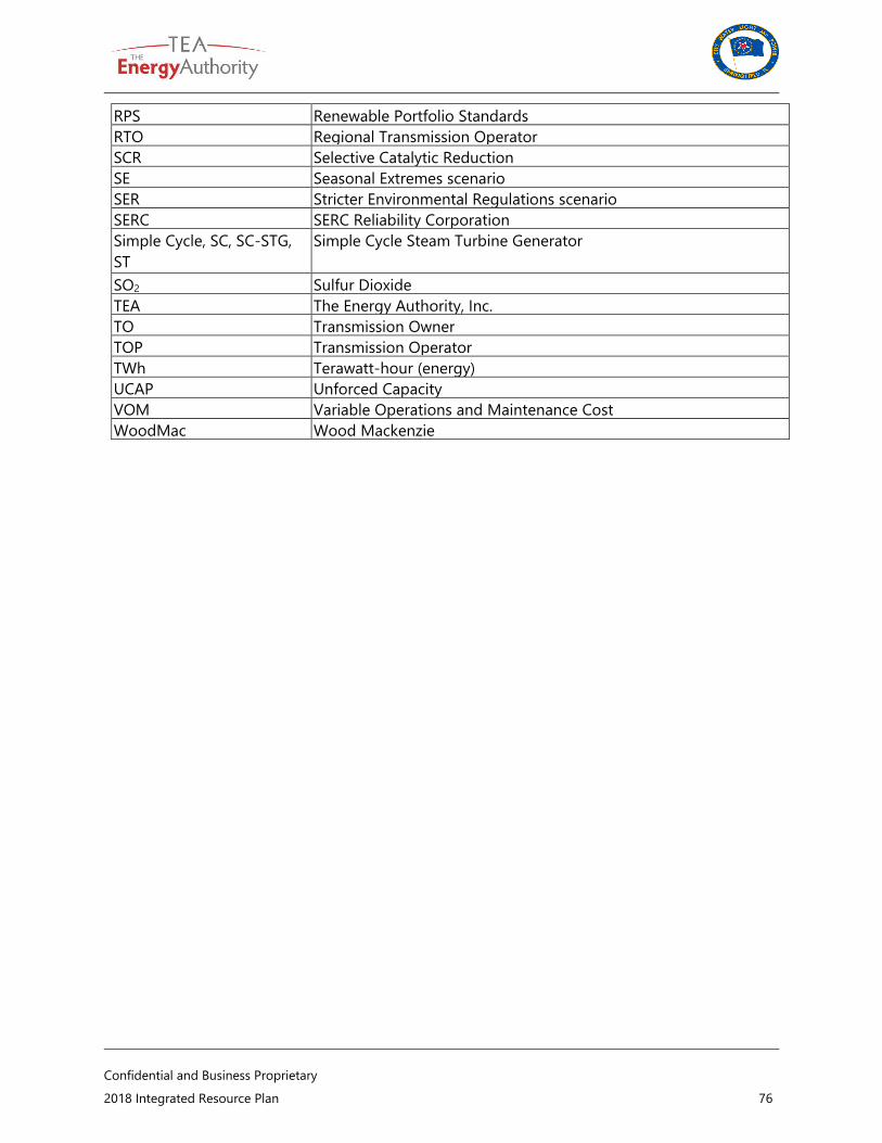
Confidential and Business Proprietary
2018 Integrated Resource Plan 76
RPS Renewable Portfolio Standards
RTO Regional Transmission Operator
SCR Selective Catalytic Reduction
SE Seasonal Extremes scenario
SER Stricter Environmental Regulations scenario
SERC SERC Reliability Corporation
Simple Cycle, SC, SC-STG,
ST
Simple Cycle Steam Turbine Generator
SO2 Sulfur Dioxide
TEA The Energy Authority, Inc.
TO Transmission Owner
TOP Transmission Operator
TWh Terawatt-hour (energy)
UCAP Unforced Capacity
VOM Variable Operations and Maintenance Cost
WoodMac Wood Mackenzie
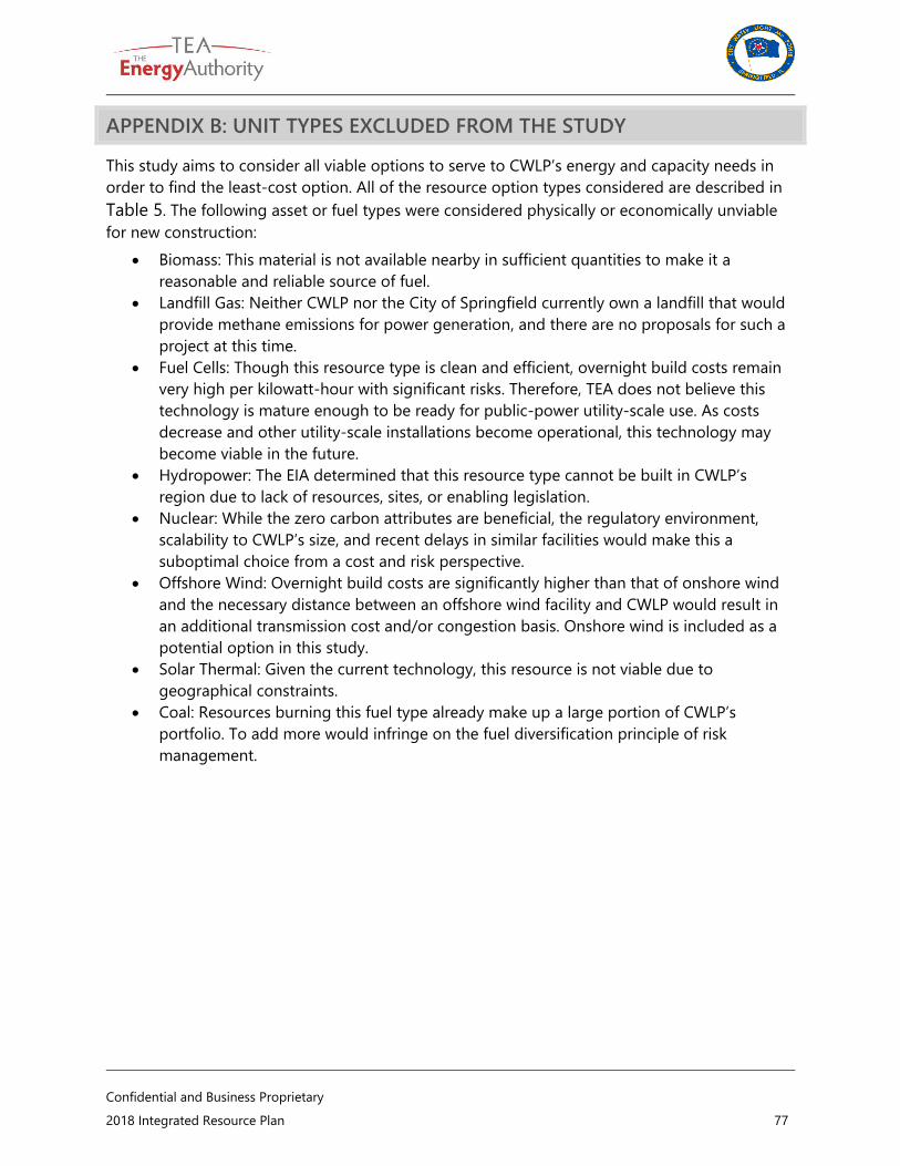
Confidential and Business Proprietary
2018 Integrated Resource Plan 77
APPENDIX B: UNIT TYPES EXCLUDED FROM THE STUDY
This study aims to consider all viable options to serve to CWLP’s energy and capacity needs in
order to find the least-cost option. All of the resource option types considered are described in
Table 5. The following asset or fuel types were considered physically or economically unviable
for new construction:
Biomass: This material is not available nearby in sufficient quantities to make it a
reasonable and reliable source of fuel.
Landfill Gas: Neither CWLP nor the City of Springfield currently own a landfill that would
provide methane emissions for power generation, and there are no proposals for such a
project at this time.
Fuel Cells: Though this resource type is clean and efficient, overnight build costs remain
very high per kilowatt-hour with significant risks. Therefore, TEA does not believe this
technology is mature enough to be ready for public-power utility-scale use. As costs
decrease and other utility-scale installations become operational, this technology may
become viable in the future.
Hydropower: The EIA determined that this resource type cannot be built in CWLP’s
region due to lack of resources, sites, or enabling legislation.
Nuclear: While the zero carbon attributes are beneficial, the regulatory environment,
scalability to CWLP’s size, and recent delays in similar facilities would make this a
suboptimal choice from a cost and risk perspective.
Offshore Wind: Overnight build costs are significantly higher than that of onshore wind
and the necessary distance between an offshore wind facility and CWLP would result in
an additional transmission cost and/or congestion basis. Onshore wind is included as a
potential option in this study.
Solar Thermal: Given the current technology, this resource is not viable due to
geographical constraints.
Coal: Resources burning this fuel type already make up a large portion of CWLP’s
portfolio. To add more would infringe on the fuel diversification principle of risk
management.

Confidential and Business Proprietary
2018 Integrated Resource Plan 78
APPENDIX C: LEVELIZED COST OF ENERGY
The levelized cost of energy (LCOE) is an industry-standard measure of cost over the life of a
resource expressed in terms of cost per MWh. LCOE typically divides the total lifetime cost of the
resource by the total lifetime output, as shown below.
LCOE =
∑ I𝑡 + M𝑡 + F𝑡
(1 + r)𝑡
𝑛
𝑡=1
∑E𝑡
(1 + r)𝑡
𝑛
𝑡=1
It = Capital investment and financing expenditures in year t
Mt = O&M expenditures in year t
Ft = Fuel expenditures in year t
Et = Electric output in year t
r = Discount rate
n = Life of system
Because this study uses four different demand and energy forecasts between all the scenarios,
LCOE is used here in conjunction with NPVRR to help illustrate the comparative costs of each
plan. For the purposes of this IRP, the calculation was slightly altered to the total plan cost (the
NPVRR) divided by the total energy usage.
LCOE =
∑ I𝑡 + M𝑡 + F𝑡 + P𝑡
(1 + r)𝑡
𝑛
𝑡=1
∑L𝑡
(1 + r)𝑡
𝑛
𝑡=1
It = Capital investment expenditures in year t, including and financing expenditures on new
resources
Mt = O&M expenditures in year t
Ft = Fuel expenditures in year t
Pt = Net market purchase costs in year t
Lt = Energy usage for load in year t
r = Discount rate
n = Length of study period

Confidential and Business Proprietary
2018 Integrated Resource Plan 79
APPENDIX D: SCENARIO ANNUAL REVENUE REQUIREMENTS
The figures in this appendix show the annual costs of each scenario by cost component. They
may be compared with Figure 27 in Section 6, which shows the same information for the
reference case.
Figure 38: AFC Scenario Annual Revenue Requirements

Confidential and Business Proprietary
2018 Integrated Resource Plan 80
Figure 39: LFC Scenario Annual Revenue Requirements
Figure 40: DET Scenario Annual Revenue Requirements

Confidential and Business Proprietary
2018 Integrated Resource Plan 81
Figure 41: FLC Scenario Annual Revenue Requirements
Figure 42: HC Scenario Annual Revenue Requirements
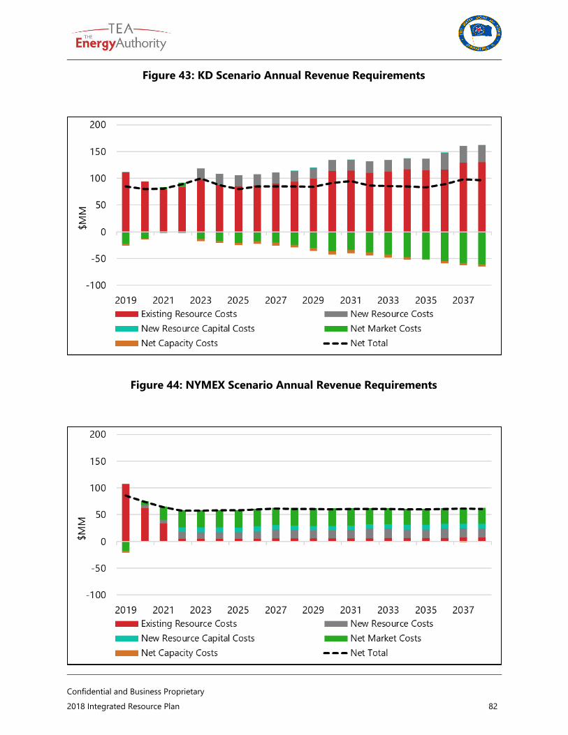
Confidential and Business Proprietary
2018 Integrated Resource Plan 82
Figure 43: KD Scenario Annual Revenue Requirements
Figure 44: NYMEX Scenario Annual Revenue Requirements
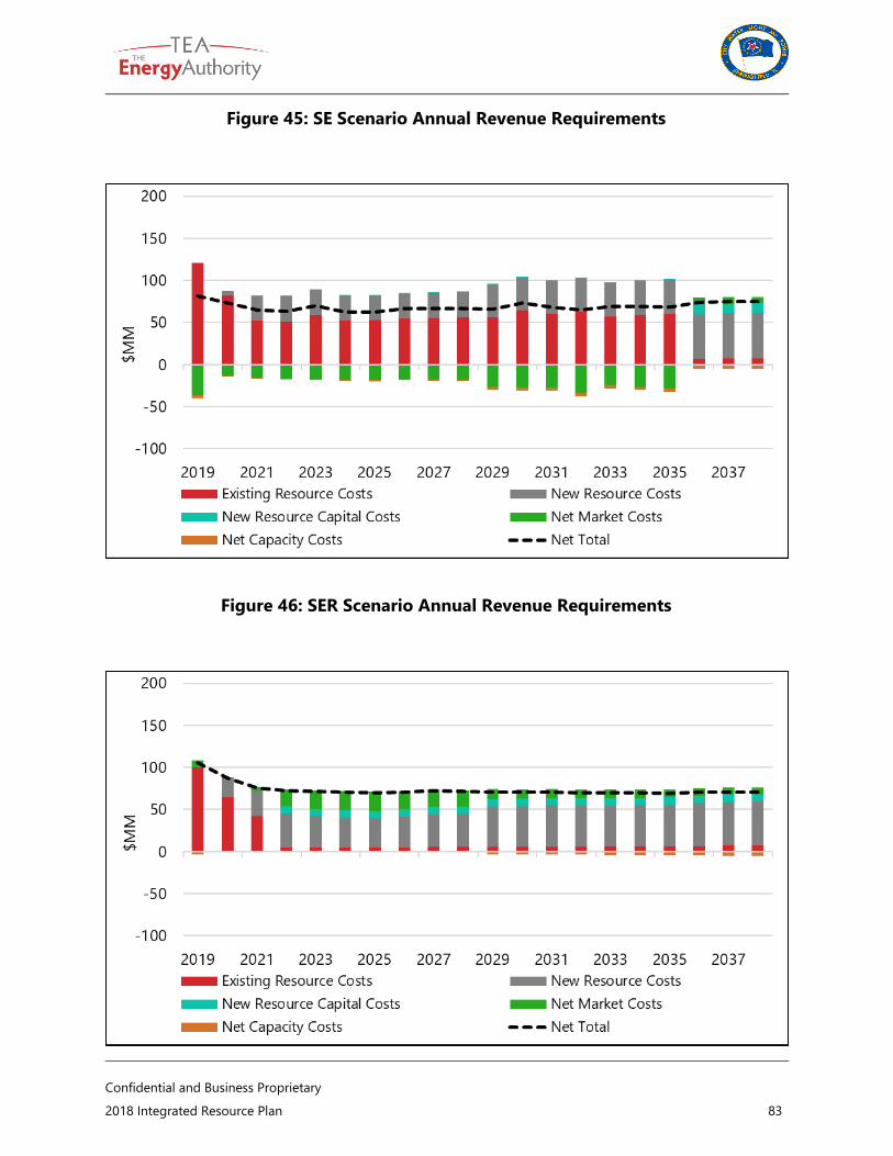
Confidential and Business Proprietary
2018 Integrated Resource Plan 83
Figure 45: SE Scenario Annual Revenue Requirements
Figure 46: SER Scenario Annual Revenue Requirements