Embed Size (px)
Citation preview

City, University of London Institutional Repository
Citation: Giaralis, A. & Spanos, P. D. (2010). Effective linear damping and stiffness coefficients of nonlinear systems for design spectrum based analysis. Soil Dynamics and Earthquake Engineering, 30(9), pp. 798-810. doi: 10.1016/j.soildyn.2010.01.012
This is the unspecified version of the paper.
This version of the publication may differ from the final published version.
Permanent repository link: http://openaccess.city.ac.uk/920/
Link to published version: http://dx.doi.org/10.1016/j.soildyn.2010.01.012
Copyright and reuse: City Research Online aims to make research outputs of City, University of London available to a wider audience. Copyright and Moral Rights remain with the author(s) and/or copyright holders. URLs from City Research Online may be freely distributed and linked to.
City Research Online: http://openaccess.city.ac.uk/ [email protected]
City Research Online

1
EFFECTIVE LINEAR DAMPING AND STIFFNESS COEFFICIENTS OF NONLINEAR
SYSTEMS FOR DESIGN SPECTRUM BASED ANALYSIS
Agathoklis Giaralis1 and Pol D. Spanos2*
1School of Engineering and Mathematical Sciences, City University London, Northampton Square, EC1V 0HB,
London, UK. E-mail: [email protected]
2L. B. Ryon Chair in Engineering, Rice University, MS 321, P.O. Box 1892, Houston, TX 77251, USA. E-mail:
ABSTRACT
A stochastic approach for obtaining reliable estimates of the peak response of
nonlinear systems to excitations specified via a design seismic spectrum is proposed. This is
achieved in an efficient manner without resorting to numerical integration of the governing
nonlinear equations of motion. First, a numerical scheme is utilized to derive a power
spectrum which is compatible in a stochastic sense with a given design spectrum. This power
spectrum is then treated as the excitation spectrum to determine effective damping and
stiffness coefficients corresponding to an equivalent linear system (ELS) via a statistical
linearization scheme. Further, the obtained coefficients are used in conjunction with the
(linear) design spectrum to estimate the peak response of the original nonlinear systems. The
cases of systems with piecewise linear stiffness nonlinearity, along with bilinear hysteretic
systems are considered. The seismic severity is specified by the elastic design spectrum
prescribed by the European aseismic code provisions (EC8). Monte Carlo simulations

2
pertaining to an ensemble of non-stationary EC8 design spectrum compatible accelerograms
are conducted to confirm that the average peak response of the nonlinear systems compare
reasonably well with that of the ELS, within the known level of accuracy furnished by the
statistical linearization method. In this manner, the proposed approach yields ELS which can
replace the original nonlinear systems in carrying out computationally efficient analyses in the
initial stages of the aseismic design of structures under severe seismic excitations specified in
terms of a design spectrum.
Keywords: Statistical linearization, design spectrum, inelastic spectrum, bilinear hysteretic,
equivalent linear system, power spectrum
1. INTRODUCTION
Contemporary code provisions favor response spectrum-based analyses for the aseismic
design of structures. For this purpose, they prescribe elastic response (design) spectra to define
the input seismic severity in terms of the peak response of linear single-degree-of-freedom
(SDOF) oscillators characterized by their natural period T and ratio of critical damping ζ (e.g.
[1]). Nevertheless, regulatory agencies allow for ordinary structures to exhibit inelastic/
hysteretic behavior (i.e. to suffer some structural damage), towards achieving cost-effective,
functional, and aesthetically acceptable designs. In a performance-based design context, the
extent of the allowable damage depends on the severity of the seismic event considered relative
to the one defined by the elastic design spectrum (e.g. [2]). This is accomplished, within the

3
common force-based aseismic design procedure, by considering reduced input seismic forces
compared to those prescribed by the elastic design spectrum by a factor R (strength reduction
factor), with the stipulation that appropriate detailing is ensured during construction so that the
structure complies with certain “performance criteria”. Inherent to the latter consideration is the
concept of ductility demand μ which is equal to the ratio of the maximum lateral deformation
attained by a yielding structure over a “nominal” yielding deformation. Thus, linear response
spectrum-based analysis can still be applied for the aseismic design of ordinary constructed
facilities by incorporating a spectrum of reduced ordinates (inelastic design spectrum) to allow
for inelastic structural behavior expressed in terms of a specified level of ductility demand.
Initiated by the work of Veletsos and Newmark [3], significant research effort has been
devoted over the past five decades to calculating the peak response of SDOF oscillators of T
natural period for small oscillations (i.e. when no yielding occurs) tracing various nonlinear
force-deformation laws for a large number of recorded ground motions pertaining to various
seismic events. This is done by numerical integration of the governing nonlinear equations of
motion. Based on such extensive numerical studies, several semi-empirical R-μ-T relations have
been proposed for obtaining inelastic response spectra from the elastic ones (see e.g. References
[4-7]). In fact, all contemporary code provisions rely on simplified versions of such relations to
define inelastic response spectra to be used for the design of structures.
Alternatively, computationally demanding inelastic time-history analyses can be
incorporated to obtain the inelastic response time-histories of nonlinear structures using
numerical integration techniques. In the aseismic design framework dictated by a specific code,
these kinds of analyses require the consideration of field recorded or artificially generated

4
seismic accelerograms conforming with certain compatibility criteria with the prescribed elastic
design spectrum (see e.g. [8]).
A considerably different approach in dealing with nonlinear systems response
determination is to employ a linearization technique. That is, to approximate the a priori
unknown response of the nonlinear systems by considering the response of an appropriately
defined “equivalent” linear system (ELS). In general, the dynamical properties of the ELS
(effective/equivalent stiffness and damping) depend on the force-deformation law of the
nonlinear system (e.g. elastic, inelastic/ hysteretic), on the input excitation (e.g. harmonic,
earthquake, stochastic etc.), and on the various assumptions made by the particular linearization
scheme. Representing a non-linear oscillator by a linear effective natural period Teq and a ratio of
critical damping ζeq facilitates the study of the underlying non-linear behavior significantly since
these effective linear properties are amenable to a clear physical interpretation. More
importantly, in obtaining the response of the nonlinear system the numerical integration of the
nonlinear equations of motion is circumvented by such a representation. This of course is
achieved at the cost of accepting certain errors due to the simplifying approximating assumptions
inherent to all linearization techniques. For instance, in the cases where the response of nonlinear
SDOF and multi-DOF systems to a stochastic excitation is of interest, the method of statistical
(or stochastic) linearization is considered the most versatile alternative to the computationally
demanding Monte Carlo analyses (see e.g. [9] and references therein). The latter analyses
involve the integration of the nonlinear equations deterministically for an appropriately derived
ensemble of time-histories statistically consistent with the considered stochastic input process.
Focusing on earthquake engineering applications, consideration of equivalent linear
oscillators derived from non-linear oscillators allows for interpreting the inelastic response

5
spectra as elastic response spectra corresponding to the effective stiffness and damping
properties of the ELS (e.g. [10]). In fact, this interpretation renders possible the development of
inelastic spectra from (Teq, ζeq)-μ-Τ relations as opposed to the previously discussed R-μ-T
relations. For example, Iwan and Gates [11] and Kwan and Billington [12] derived (Teq, ζeq)-μ-Τ
relations via numerical integration of various non-linear oscillators exposed to certain field
recorded strong ground motions. Furthermore, Gulkan and Sozen [13] and Shibata and Sozen
[14] suggested the use of ELS, derived from pertinent experimental results on single and multi
storey R/C frames, as a tool for aseismic design of R/C structures. Based on the above concepts,
the tool of an equivalent linear SDOF “substitute” structure is incorporated to account for the
inelastic behavior of SDOF and MDOF structures in various contemporary methodologies for the
aseismic design and the assessment of the seismic vulnerability of structures (see e.g. [15-18]).
Clearly, the development of efficient linearization schemes accounting for the input seismic
action in terms of a given design spectrum is critical and timely.
Jennings [19] considered and compared six early deterministic linearization methods,
assuming harmonic excitation and steady-state response conditions. Further, Iwan and Gates [20]
assessed the potential of various linearization techniques to estimate the peak response of certain
SDOF hysteretic oscillators exposed to strong ground motion. This was done vis-à-vis numerical
results obtained by integrating the nonlinear equations of motion for an ensemble of 12 recorded
accelerograms. Similarly, Hadjian [21] compared the formulae for defining equivalent linear
properties resulting from several linearization techniques for elasto-plastic SDOF hysteretic
systems. All the linearization techniques considered in these early studies define
deterministically the ELSs without considering the statistical attributes of the seismic hazard
explicitly.

6
More recently, Koliopoulos et al. [22] pursued a comparative assessment of the
applicability of certain linearization schemes for the case of bilinear hysteretic SDOF systems. In
this case a small ensemble (9) of artificial accelerograms whose average response spectra was
relatively close to a specific design spectrum prescribed by the European aseismic code
provisions (EC8) was used for the numerical validation of the techniques considered. One of
these schemes involved random vibration-based linearization relying on the solution of an
underlying Fokker-Planck equation, necessitating the assumption of white noise input: a limiting
one for representing strong ground motion excitations.
Furthermore, Basu and Gupta [23] derived inelastic spectra pertaining to certain recorded
seismic accelerograms also based on a statistical linearization formulation. This formulation
required the minimization of the expected value of the square difference (error) between the
considered nonlinear equation of motion and the corresponding (target) equivalent linear with
respect to the dynamical properties of the ELS. The associated expected values were computed
based on the distribution of the peak response of the ELS excited by a Gaussian stationary
process. A piecewise linear non-hysteretic type of nonlinearity was considered with a fixed value
for the yielding displacement selected so that the system experiences mild nonlinear behavior.
An attempt to predict the lower order displacement peaks and to develop constant cumulative
damage spectra was also made assuming a Kanai-Tajimi filtered white noise excitation. Later,
the formulation was applied for the case of bilinear hysteretic oscillators [24]. However, the
scope of both of the aforementioned studies was to estimate the damage accumulation of the
underlying nonlinear systems. Thus not special attention was given to the equivalent linear
parameters which were treated as by-products of the statistical linearization formulation
followed.

7
Moreover, in Miranda and Ruiz-García [25] the performance of four deterministic
linearization schemes, along with two popular R-μ-Τ relations, were evaluated to obtain peak
deformations of certain hysteretic SDOF systems. Special attention was given to quantifying the
error of the estimated maximum responses versus results from a comprehensive Monte Carlo
analysis involving the numerical integration of the nonlinear systems for a bank of 264 recorded
accelerograms.
In a study concerning the response of secondary systems founded on SDOF nonlinear
systems, Politopoulos and Feau [26] proposed two different schemes to derive equivalent linear
parameters. The first, concerns hysteretic perfectly elasto-plastic SDOF systems and involves a
least square fit of linear transfer functions to power spectra estimated from response data of
nonlinear systems obtained from Monte Carlo analyses. Clearly, this procedure does not
circumvent the numerical integration of the nonlinear equations of motion while it involves
certain approximations associated with spectral estimation and curve fitting considerations. The
second, pertains to a class of nonlinear elastic systems subject to white noise excitation and
utilizes a special statistical linearization procedure treating the equivalent linear stiffness
parameter as a random variable. From a practical viewpoint, both the white noise excitation
assumption and the probabilistic nature of the equivalent linear stiffness parameter considered
limit, rather significantly, the merit of these proposed linearization methods.
Notably, the potential advantages of focusing on the ELS derived from the method of
statistical linearization considering input processes consistent with elastic design spectra seems
to have been overlooked in the published literature. In this paper, a design spectrum compatible
power spectrum is considered in conjunction with appropriate statistical linearization schemes as
a surrogate for determining the peak seismic response of nonlinear systems. It is emphasized that

8
the purpose of the present work is not to assess the accuracy of the statistical linearization
technique, a well-studied theme in the literature (see e.g [9] and references therein). Instead, it
proposes a novel approach to estimate inelastic response spectral ordinates from a given family
of elastic spectra for various damping ratios without resorting to numerical integration of the
underlying nonlinear equations of motion. In this manner, the need to consider field recorded
accelerograms of similar characteristics to the ones that have been used in the definition of the
considered design spectrum is circumvented. Furthermore, the inherent probabilistic nature of
the excitation is explicitly accounted for. Note that the stationarity assumption in the surrogate
model of the strong ground motion input renders the statistical linearization step quite efficient,
while it is not particularly restrictive in accounting for the physical aspects of strong ground
motions. In fact, it has been argued that stationary power spectra consistent with a given
response/design spectrum accounts implicitly for the transient attributes of the response of
seismically excited structures as these reflect on the response/design spectrum [27].
Figure 1.
For clarity, the proposed approach is qualitatively presented in the flowchart of Figure 1.
Clearly, the main steps of the approach encompass the derivation of a design spectrum
compatible power spectrum, an issue that has been extensively studied in the open literature (e.g.
[28-31]), and the application of the statistical linearization method (see e.g. [9, 32-33]). To this
end, in section 2 an efficient method for deriving design spectrum compatible power spectrum is
considered. Further, section 3 reviews the pertinent mathematical formulae for deriving ELS via
the statistical linearization method for viscously damped SDOF oscillators characterized by
hardening piecewise linear elastic, and bilinear hysteretic restoring force-deformation laws.
Section 4 provides numerical results supporting the effectiveness and the practical usefulness of

9
the proposed approach in conjunction with the design spectrum prescribed by EC8 [2]. Finally,
section 5 includes pertinent concluding remarks.
2. DERIVATION OF RESPONSE SPECTRUM COMPATIBLE POWER SPECTRA
The core equation for relating a design/response pseudo-acceleration seismic spectrum Sα
to a one-sided power spectrum G(ω) representing a Gaussian stationary process g(t) in the
frequency domain reads (e.g. [34])
( ) 2, ,0,,a j n j G j j GS ω ζ η ω λ= . (1)
In the above equation λj,m,G denotes the spectral moment of order m of the stationary response of
a linear single-degree-of-freedom (SDOF) mass-spring-damper system of natural frequency ωj
and damping ratio ζn base-excited by the process g(t). Namely,
( )
( ) ( ), , 2 22 20 2
m
j m G
j n j
Gd
ω ωλ ω
ω ω ζ ωω
∞
=− +
∫ . (2)
Furthermore, the “peak factor” ηj,G appearing in Equation (1) is the critical parameter
establishing the equivalence, with probability of exceedance p, between the Sa and G(ω) [34].
Specifically, it represents the factor by which the standard deviation of the response of the
considered SDOF oscillator must be multiplied to predict the level Sa below which the peak
response of the oscillator will remain, with probability p, throughout the duration of the input
process Ts. The exact determination of ηj,G is associated with the first passage problem which
involves the evaluation of the probability that the response of a linear SDOF oscillator does not
cross a certain amplitude level (barrier) within the duration Ts (see e.g. [35]). A closed form
solution for this problem is not available. Herein, the following semi-empirical formula for the

10
calculation of the peak factor is adopted which is known to be reasonably reliable for earthquake
engineering applications ([34, 36])
( )( ){ }1.2, , , ,2 ln 2 1 exp ln 2j G j G j G j Gv q vη π⎡ ⎤= − −⎢ ⎥⎣ ⎦
, (3)
where
( ) 1,2,,
,0,
ln2
j Gsj G
j G
Tv pλ
π λ−= − , (4)
and
2,1,
,,0, ,2,
1 j Gj G
j G j G
qλ
λ λ= − . (5)
For the purposes of this study, it is appropriate to set the probability p equal to 0.5 in
Equation (4). Under this assumption, Equation (1) prescribes the following compatibility
criterion: considering an ensemble of stationary samples of the process g(t) half of the population
of their response spectra will lie below Sa (i.e. Sa is the median response spectrum). A
computationally efficient numerical scheme is used to derive a non-parametric power spectrum
G(ω) satisfying the aforementioned criterion for a given pseudo-acceleration design spectrum by
solving the “inverse” stochastic dynamics problem governed by Equations (1) to (5). Compared
to other methods utilized in the literature in a similar context, this scheme does not require
iterations to be performed as in [28-29], and does not involve the solution of an optimization
problem as in [29-30].
In particular, the adopted scheme relies on the following approximate formula to obtain a
reliable estimate for the response variance of a lightly damped SDOF system subject to a
relatively broadband excitation [34]

11
( ) ( ),0, 3 4
0
114
jj
j Gj n j
GG d
ωω πλ ω ωω ζ ω
⎛ ⎞= − +⎜ ⎟
⎝ ⎠∫ . (6)
Approximating the integral in Equation (6) by a discrete summation, substituting Equation (6) in
Equation (1), and appropriately rearranging the resulting terms yields [31, 34]
( ) [ ]
2 1
0211 ,
0
,4 ,4
0 , 0
jj n
k jkj n j j Nj
j
SG
Gα ω ζζ ω ω ω ω
ω π ζ ω ηω
ω ω
−
=−
⎧ ⎛ ⎞⎪ ⎜ ⎟− Δ >⎪ ⎜ ⎟−⎡ ⎤ = ⎨⎣ ⎦ ⎝ ⎠⎪
≤ ≤⎪⎩
∑ . (7)
Τhe latter equation establish an approximate numerical scheme to recursively evaluate G(ω) at a
specific set of equally spaced by Δω (in rad/sec) natural frequencies ωj= ω0+ (j-0.5)Δω; j=
1,2,…,M where ω0 denotes the lowest bound of the existence domain of Equation (3) [31].
Specifically, ω0 should be set equal to the lowest value of the natural frequency ωn which
simultaneously satisfies the conditions
( ),ln 2 0j Nv ≥ , (8)
and
( )( ){ }1.2, , ,ln 2 1 exp ln 2 0j N j N j Nv q vπ⎡ ⎤− − ≥⎢ ⎥⎣ ⎦
. (9)
Obviously, in implementing the above scheme the peak factors ηj,N need to be calculated
for an input power spectrum N(ω) which has to be a priori assumed without knowledge of G(ω).
The duration of the underlying stationary process characterized by N(ω) is assumed equal to the
duration Ts of g(t). Conveniently, the value of ηj,N is not very sensitive to the shape of the
spectrum N(ω) (see e.g. [36]). This observation is justified by the fact that the evaluation of the
peak factor (Equations (2) to (5)), involves ratios of integrals of the product of the input power
spectrum with the squared modulus of the frequency response function of the various SDOF
systems considered over the whole range of frequencies. The validity of this assertion is verified
12
in a following section using numerical results pertaining to three different shapes of N(ω). These
are the unit amplitude white noise (WN) spectrum
( ) 1 ; 0 bN ω ω ω= ≤ ≤ , (10)
the Kanai-Tajimi (KT) spectrum [37]
( )
2
2
22 2
2
1 4; 0
1 4
gg
b
gg g
N
ωζω
ω ω ωω ωζω ω
⎛ ⎞+ ⎜ ⎟⎜ ⎟
⎝ ⎠= ≤ ≤⎛ ⎞⎛ ⎞ ⎛ ⎞⎜ ⎟− +⎜ ⎟ ⎜ ⎟⎜ ⎟ ⎜ ⎟⎜ ⎟⎝ ⎠ ⎝ ⎠⎝ ⎠
, (11)
and the Clough-Penzien (CP) spectrum [38]
( )
4 2
2
2 22 2 2 2
2 2
1 4; 0
1 4 1 4
gf g
b
f gf f g g
N
ω ωζω ω
ω ω ωω ω ω ωζ ζω ω ω ω
⎛ ⎞ ⎛ ⎞+⎜ ⎟ ⎜ ⎟⎜ ⎟ ⎜ ⎟
⎝ ⎠ ⎝ ⎠= ≤ ≤⎛ ⎞ ⎛ ⎞⎛ ⎞ ⎛ ⎞ ⎛ ⎞ ⎛ ⎞⎜ ⎟ ⎜ ⎟− + − +⎜ ⎟ ⎜ ⎟ ⎜ ⎟ ⎜ ⎟⎜ ⎟ ⎜ ⎟ ⎜ ⎟ ⎜ ⎟⎜ ⎟ ⎜ ⎟⎝ ⎠ ⎝ ⎠ ⎝ ⎠ ⎝ ⎠⎝ ⎠ ⎝ ⎠
, (12)
where ωg, ζg, ωf, and ζf are predefined constant parameters, and ωb is the largest frequency of
interest. The values of the parameters ωg, ζg reflect the filtering effects of the surface soil
deposits on the propagating seismic waves during an earthquake event. Thus, they should be
judicially chosen based on the soil conditions associated with the given (target) design spectrum.
The parameters ωf, ζf control the shape of the high-pass filter incorporated in the CP spectrum to
suppress the low frequencies allowed by the KT spectrum and their values should be selected
accordingly. More detailed discussions on the spectral forms of Equations (11) and (12) can be
found in [8] and the references therein.
To this end, it is noted that the evaluation of the spectral moment integrals defined by
Equation (2) for the input spectra given by the Equations (10) to (12) can be performed either
numerically using appropriate quadrature rules or analytically. In the latter case, the residue

13
theorem for complex integration can be employed [36]. Alternatively, these response spectral
moments can be obtained by solving linear systems of equations derived from application of the
Hilbert transform on the governing differential equations of motion as it has been shown by
Spanos and Miller [39]. For the simplest case of N(ω) being unit strength white noise (WN) the
following closed form expressions for the quantities in Equations (4) and (5) hold
( ) ( ) 1, 1 ln
2s
j N n jTv pωπ
−= = − , (13)
2
1, 1 2 2
1 21 1 tan1 1
j Nq ζζ π ζ
−=
⎛ ⎞⎜ ⎟= − −⎜ ⎟− −⎝ ⎠
. (14)
Regarding the conditions of Equations (8) and (9), pertinent plots shown in Figure 2(a)
reveal that Equation (9) defines a more stringent criterion which is satisfied for relatively small
values of ω0 for the cases that N(ω) assumes a WN and a KT spectral form (Figure 2(b)). Results
from extensive numerical experimentation, similar to those presented in Figure 1 indicate that for
the range of values of the KT parameters, ωg and ζg, of practical interest, the admissible values
for ω0 coincide with those for the WN input spectrum. Interestingly, for the CP spectrum ω0 is
always zero since the left hand side of Equations (8) and (9) are positive everywhere (see also
Figure 2(a)). This result is associated with the fact that the CP spectrum vanishes as ω→0.
Figure 2.
Note that upon determining the discrete power spectrum G[ωj] by Equation (7) the
associated pseudo-acceleration response spectrum D[ωj,ζ] can be computed in a straightforward
manner using Equations (1) to (5). For this purpose, the first three spectral moments of the
14
response of a SDOF system excited by a process characterized by a power spectrum known at
equally spaced frequencies can be evaluated by the formulas reported in [29, 40], which are
included in the Appendix for completeness.
Incidentally, if so desired, the initially obtained discrete power spectrum G[ωj] can be
further modified iteratively to improve the matching of the associated response spectrum D[ωj,ζ]
with the target design spectrum Sα according to the equation written at the v-th iteration (e.g.
[27])
( ) ( )( )
2
1 ,
,a jv v
j j vj
SG G
D
ω ζω ω
ω ζ+
⎛ ⎞⎡ ⎤⎣ ⎦⎜ ⎟⎡ ⎤ ⎡ ⎤=⎣ ⎦ ⎣ ⎦ ⎜ ⎟⎡ ⎤⎣ ⎦⎝ ⎠. (15)
3. BACKGROUND ON THE STATISTICAL LINEARIZATION METHOD
Consider a unit-mass viscously-damped quiescent SDOF system with a non-linear
restoring force component base-excited by the stationary zero-mean acceleration process g(t)
characterized in the frequency domain by the power spectrum G(ω). The equation of motion of
this system reads
( ) ( ) ( ) ( ) ( ) ( )22 , ; 0 0 0n n nx t x t x x g t x xζ ω ω ϕ+ + = − = = , (16)
in which x(t) is the system deformation (displacement trace of the system relative to the motion
of the ground), ωn is the system natural frequency for small deformations, ζn is the ratio of
critical viscous damping, and ( ),x xϕ is a nonlinear function governing the restoring force-
deformation law; the dot over a symbol signifies differentiation with respect to time t.
The statistical linearization method utilizes the response process y of an equivalent linear
system (ELS) of natural frequency ωeq and damping ratio ζeq given by the equation

15
( ) ( ) ( ) ( ) ( ) ( )22 ; 0 0 0eq eq eqy t y t y t g t y yζ ω ω+ + = − = = , (17)
to approximate the process x, that is, the response of the non-linear oscillator of Equation (16)
[9]. According to the original and most widely-used form of statistical linearization the above
linear system is defined by minimizing the expected value of the difference (error) between
Equations (16) and (17) in a least square sense with respect to the quantities ωeq and ζeq (i.e. the
effective dynamical properties of the ELS), (see e.g. [9, 32-33]). This criterion yields the
following expressions for the effective linear properties [9]
( ){ }{ }
22
,eq
E x x xE xϕ
ω = , (18)
and
( ){ }{ }2
,n
eq neq
E x x xE xϕωζ ζ
ω= + , (19)
where E{•} denotes the mathematical expectation operator. In this junction, it is commonly
assumed that the unknown distribution of the response process x of the non-linear oscillator can
be approximated, for the purpose of evaluating the expected values, by a zero-mean Gaussian
process. Furthermore, it is also assumed that the variances of the processes x and y are equal ([9,
33]). The latter suggests that
{ } ( )( ) ( )
2,0, 2 22 2
0 2eq G
eq eq eq
GE x d
ωλ ω
ω ω ζ ωω
∞
= =− +
∫ , (20)
and
{ } ( )( ) ( )
22
,2, 2 22 20 2
eq G
eq eq eq
GE x d
ω ωλ ω
ω ω ζ ωω
∞
= =− +
∫ (21)

16
in Equations (18) and (19). Under the aforementioned assumptions, Equations (18) and (19) can
be simplified as [9]
( )2 ,
eq
x xE
xϕ
ω∂⎧ ⎫
= ⎨ ⎬∂⎩ ⎭, (22)
and
( ),n
eq neq
x xE
xϕωζ ζ
ω∂⎧ ⎫
= + ⎨ ⎬∂⎩ ⎭. (23)
For many nonlinear force-deformation laws of practical interest the above formulae assumption
leads to closed-form expressions which facilitate significantly the application of the statistical
linearization method [9]. In any case, Equations (20) to (23) establish a system of nonlinear
equations that needs to be simultaneously satisfied. Typically, this is achieved via a numerical
iterative scheme [9]. Conveniently for the purposes of the proposed approach, G(ω) is a non-
parametric power spectrum known at a specific set of equally-spaced frequencies and thus the
integrals in Equations (22) and (23) can be evaluated at each iteration using the closed-form
formulas included in the Appendix.
It is noted that statistical linearization formulations using alternative criteria to minimize
the error between Equations (16) and (17) have been proposed in the literature (e.g. [23, 33, 41-
43]), while significant research effort has been also devoted in relaxing the aforementioned
Gaussian distribution assumption (e.g. [44, 45]). However, such considerations involve
computationally intensive iterative numerical schemes requiring the calculation of integrals
which are not amenable to analytical treatment, without necessarily yielding results of
substantially increased accuracy (see e.g. [23, 33, 43]). Since simplicity and computational
efficiency are primary objectives in the herein proposed approach, the classical statistical
linearization method is adopted in all of the ensuing analytical and numerical results to obtain

17
equivalent linear properties by minimizing the squared difference between the nonlinear and the
equivalent linear system. Further, the assumption that the distribution of the nonlinear response
can be approximated by a Gaussian one is adopted to compute the mathematical expectations in
Equations (22) and (23). It should be clear from the preceding comments that the effective linear
properties ωeq and ζeq obtained through iterative solution of Equations (20) to (23) depend
explicitly on the input power spectrum G(ω). In the framework of the proposed approach G(ω) is
compatible with a given design spectrum and thus these ωeq and ζeq are related in a statistical
sense with the latter spectrum in a straightforward manner. This constitutes the main advantage
of the herein developed approach over the common equivalent linearization techniques used in
various aseismic design procedures which define ELSs without accounting for the input seismic
action as defined by regulatory agencies by means of design spectra (see e.g. [18, 46-48]. In the
remainder of this section certain nonlinear restoring force-deformation laws of practical interest
are discussed, and the pertinent formulas to obtain the related ωeq and ζeq are reported.
3.1. Piecewise linear restoring force
Consider a hardening non-linear elastic oscillator characterized by a piecewise linear
restoring force consisted of two branches. Let α>1 be the stiffness (rigidity) ratio between the
branches and xy be the critical deformation for which a change of stiffness occurs as shown in
Figure 3(a). The equation of motion for such a system is obtained by substituting in Equation
(16):
( )( ) ( ) ( )
;
sgn 1 ; sgny
y y
x x xx
ax x x x x xϕ
α
⎧ ≤⎪= ⎨+ − >⎪⎩
, (24)

18
where sgn(•) symbolizes the signum function, namely, sgn(x)= 1 for x>0 and sgn(x)= -1 for x<0.
Figure 3.
In practical terms, the restoring force of Equation (24) can be considered in the context of
preliminary aseismic design procedures in several cases. These include accounting for the
pounding/impact effect in structural members such as between deck elements at expansion joints
along the longitudinal direction of bridges (e.g. [49]), and between adjacent buildings (e.g. [50-
51]). They also include cases of structures whose lateral movement is restricted via “stop-
supports” and restrainers such as in above-ground pipelines along their transversal direction (e.g.
[52]), and in seismically isolated structures (e.g. [53]). In this respect, the deformation xy is
construed as the clearance/distance between structural members or between structures and their
surroundings, while the ratio α reflects the increase in the overall structural stiffness after impact.
Substitution of Equation (24) in Equations (22) and (23) yield the following expressions
for the parameters of the ELS associated with a nonlinear oscillator with piecewise linear
restoring force
( )2 2
,0,
1 ,2
yeq n
eq G
xa a erfω ω
λ
⎛ ⎞⎛ ⎞⎜ ⎟⎜ ⎟= + −
⎜ ⎟⎜ ⎟⎝ ⎠⎝ ⎠ (25)
and
neq
eq
ωζ ζω
= , (26)
in which erf (•) denotes the error function defined as

19
( ) ( )2
0
2 expu
erf u v dvπ
= −∫ . (27)
Clearly, given a certain nonlinear oscillator with piecewise linear restoring force defined by a set
of values for ωn, ζn, a, and xy or equivalently R (see Figure 3(a)), excited by a specific design
spectrum compatible G(ω), a set of linear parameters ωeq and ζeq can be computed by iteratively
solving Equations (20), (25), and (26) [9].
3.2. Bilinear hysteretic restoring force
Of particular interest in the aseismic design of structures is the bilinear hysteretic force-
deformation law show in Figure 3(b) which is the simplest model to capture the hysteretic
behavior of structural members and structures under seismic excitation (see e.g. [7, 11, 14, 51,
54]). For instance, it is a common practice to model the inelastic behavior of structures, including
multi-storey buildings and bridges, exposed to strong ground motion by viscously damped
bilinear hysteretic SDOF oscillators in the context of non-linear static analyses (see e.g. [18, 47])
and of performance/displacement-based design procedures (e.g. [15-17]). The governing
equation of motion of such an oscillator can be mathematically expressed with the aid of an
auxiliary state z by substituting in Equation (16) [55]
( ) ( ), 1x x ax a zϕ = + − , (28)
where
( ) ( ) ( ) ( ) ( ), 1 y yz x x x U x U z x U x U z x⎡ ⎤= − − − − − −⎣ ⎦ , (29)

20
in which xy is the yielding deformation and α<1 is the post-yield to pre-yield (rigidity) ratio, and
U(•) denotes the Heaviside step function, namely, U(v)= 1 for v≥0, and U(v)= 0 for v= 0.
Adopting the assumptions of the classical statistical linearization method and assuming
that the response of the nonlinear system is narrowband (i.e. is dominated by a slowly varying in
time apparent frequency) effective parameters of an ELS corresponding to a given viscously
damped bilinear hysteretic SDOF system, are obtained via the formulae (e.g. [9, 32])
( ) 2
2 23
1
8 1 1 11 1expeq n
a vv dvv v
ω ωπ θ θ
∞⎧ ⎫− ⎛ ⎞−⎪ ⎪⎛ ⎞= − + −⎨ ⎬⎜ ⎟⎜ ⎟⎝ ⎠⎪ ⎪⎝ ⎠⎩ ⎭∫ , (30)
and
2
1 11n neq n
eq eq
a erfω ωζ ζω ω πθ θ
⎛ ⎞ ⎛ ⎞− ⎛ ⎞= + −⎜ ⎟ ⎜ ⎟⎜ ⎟⎜ ⎟ ⎝ ⎠⎝ ⎠⎝ ⎠, (31)
where
,0,22 eq G
yxλ
θ = . (32)
As in the previous case considered, iterations need to be performed to numerically derive
equivalent linear properties ωeq and ζeq, from Equations (20), and (30) to (32) to approximate
statistically the response of a certain bilinear hysteretic oscillator defined by the parameters ωn,
ζn, a, and xy or equivalently R (see Figure 3(b)), excited by a specific design spectrum compatible
G(ω). Note that in this case the equivalent damping expression (Equation (31)) includes an
additional term which accounts for the energy dissipation in the nonlinear system due to
hysteresis.

21
4. NUMERICAL APPLICATION TO THE EC8 DESIGN SPECTRUM
4.1. EC8 design spectrum compatible power spectra
Consider the pseudo-acceleration design spectrum prescribed by the European aseismic
code provisions (EC8) for soil conditions B, damping ratio ζn= 5%, and peak ground acceleration
equal to 36% the acceleration of the gravity (gray thick line in Figure 4(b)) as the given/ target
spectrum [2]. Figure 4(a) includes discrete power spectra compatible with this target spectrum
computed by means of Equation (7) for the three input spectral shapes N(ω) considered in
section 2, namely white noise (WΝ) (Equation (10)), Kanai-Tajimi (KT) (Equation (11)), and
Clough-Penzien (CP) (Equation (12)). The duration Ts is taken equal to 20sec, while the
discretization step is set equal to Δω= 0.1rad/sec. The requisite parameters for the definition of
the KT and CP N(ω) spectra used are ζg= 0.78, ωg= 13.18rad/sec, ζf= 0.88, and ωf= 3.13rad/sec
reported in a recent work by [8]. These values pertain to a parametric CP type evolutionary
power spectrum compatible with the herein considered EC8 target spectrum. Furthermore,
Figure 4(a) shows an iteratively modified power spectrum computed by means of Equation (15)
after four iterations assuming as the “seed” spectrum the aforementioned WN based spectrum
which is the simplest and computationally least demanding case of a spectrum that can be
obtained utilizing Equation (7).
Figure 4.
The associated with the above power spectra pseudo-acceleration response spectra
calculated analytically by Equations (1) to (5) are plotted in Figure 4(b) and compared with the

22
target spectrum. As it can be seen in the latter figure, consideration of more elaborate input
spectral shapes N(ω) in Equation (7) results in somewhat different power spectra attaining
response spectra which achieve slightly better matching with the target design spectrum. Similar
results can be found in Giaralis [56] for EC8 design spectra pertaining to all soil types as
prescribed by the European aseismic regulations. However, the iteratively matched power
spectrum which attains a notably more resonant (“spiky”) shape compared to the power spectra
computed from Equation (7) without any additional iterations performed, achieves the best
agreement with the target spectrum. More importantly, this iteratively modified WN based
spectrum is computationally less costly to obtain compared to the KT and the CP based spectra
considered herein which involve the calculation of more complex response spectral moments as
it has been discussed in section 2 (see also [36, 39]). Thus, in the context of an efficient
algorithmic determination of design spectrum compatible power spectra, it is suggested to
perform a reasonable number of iterations via Equation (15); as a “seed” (i.e. initial estimate) a
non-parametric power spectrum obtained from Equation (7) assuming a WN N(ω) spectrum can
be used.
In Figure 4(c), pertinent results are shown associated with a Monte Carlo analysis
conducted to assess the achieved level of compatibility of the aforementioned modified power
spectrum with the target spectrum in terms of the criterion posed by Equation (1) for p= 0.5 (see
also section 2). Specifically, an ensemble of 1000 stationary signals of 20sec duration each
compatible with the iteratively modified power spectrum of Figure 4(a) are generated using an
auto-regressive-moving-average (ARMA) filtering technique [57]. The response spectra of these
signals are calculated [58] and the median spectral ordinates are compared with the EC8 target
design spectrum in Figure 4(c). The cross-ensemble minimum and maximum spectral ordinates
23
are also included to illustrate the statistical nature of the analysis. Evidently, the criterion posed
by Equation (1) is satisfactorily met, within engineering precision, by the iteratively modified
power spectrum.
4.2. Equivalent linear systems and assessment via Monte Carlo analyses
In this subsection, the applicability of the proposed approach to estimate the maximum
deformations of various stiffening piecewise linear elastic and bilinear hysteretic SDOF
oscillators is illustrated. To this aim, the iteratively modified power spectrum of Figure 4(a) is
used as a surrogate for determining equivalent linear systems (ELS) of natural period Teq and of
ratio of critical damping ζeq associated with the aforementioned nonlinear oscillators in the
context of the statistical linearization method. Furthermore, Monte Carlo simulations pertaining
to an ensemble of 40 non-stationary artificial accelerograms compatible with the previously
defined EC8 design spectrum are conducted. This is done to confirm that the average peak
response of the nonlinear systems compares reasonably well with those of the ELS. As shown in
Figure 5 the ensemble average pseudo-acceleration spectrum of these accelerograms seismic
signals is in a quite close agreement with the considered EC8 spectrum. These seismic signals
have been generated by a wavelet-based stochastic approach recently proposed by the authors
[8].
Figure 5.
In particular, Figure 6(a) to Figure 6(f) provide the properties of the ELSs (Teq and ζeq)
obtained by iteratively solving Equations (20), (25), and (26) for piecewise linear oscillators.
24
This is done for various yielding displacements xy, natural periods Tn, rigidity ratios α, and for a
fixed ratio of critical damping ζn= 0.05 exposed to the iteratively modified power spectrum of
Figure 4(a). Note that these properties are plotted against the ductility μ since this a normalized
quantity of interest expressing the demand of structural performance imposed by the input
seismic action in aseismic design practice (see also Figure 3). For the purposes of this study the
ductility μ is computed as the ratio of the average peak response of each ELS exposed to the
ensemble of the seismic signals of Figure 5 over the yielding displacement xy of the
corresponding non-linear system. As expected, systems of the same rigidity ratio α exhibiting
more severe non-linear behavior in terms of higher ductility demand, or systems of the same
level of ductility demand characterized by a higher rigidity ratio α yield stiffer ELS (i.e. ELS of
decreased natural period Teq). The equivalent viscous damping ζeq changes accordingly since by
definition it is dependent on the natural frequency of the ELS (see also Equation (26)).
In Figure 6(g) to Figure 6(i) the aforementioned ductility demands are plotted for each
considered ELS (lines of various types) versus the strength reduction factor R defined in Figure
3. These R factors are computed as the ratio of the average peak response of the infinitely linear
system corresponding to the various considered Tn values excited by the aforementioned
ensemble of signals over the yielding force fy of the corresponding non-linear system (see also
Figure 3a). Moreover, in Figure 6(g) to Figure 6(i) the average ductility demand μ obtained via
numerical integration of the considered non-linear systems with piecewise linear restoring force
(dots of various shapes) subject to the ensemble of the accelerograms of Figure 5 are also
included. For this task, the standard constant acceleration Newmark’s method, incorporating an
iterative Newton-Raphson algorithm to treat locally the discontinuities of the piecewise linear
force-deformation law, has been used (see e.g. [1]).
25
In general, the R-μ-Tn relations of Figure 6(g) to Figure 6(i) derived from the ELS and
from the corresponding systems with piecewise linear type of stiffness nonlinearity as described
above compare well for the cases considered. Clearly, this fact demonstrates the reliability of the
ELS obtained via the proposed approach to estimate the peak deformations of the non-linear
systems subject to seismic action defined by means of the given design spectrum.
Figure 6.
Similarly to the case of the piecewise linear oscillators, equivalent linear properties
corresponding to bilinear hysteretic oscillators have been determined. This has been done for
bilinear oscillators of various yielding displacements xy, natural periods Tn, and for ζn= 0.05
excited by the iteratively modified EC8 compatible power spectrum of Figure 4(a). The obtained
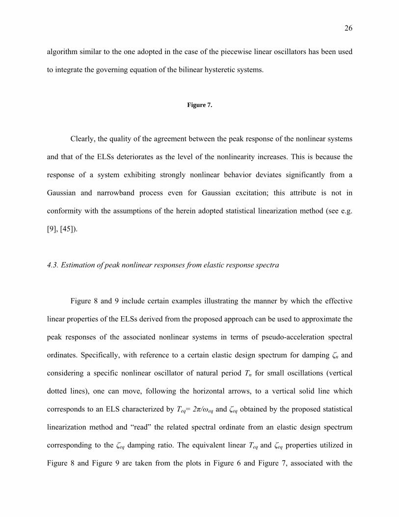
equivalent linear properties are plotted in Figure 7(a) and Figure 7(b) versus the ductility μ. The
rigidity ratio α is taken equal to 0.5. These properties have been derived by iteratively solving
Equations (20) and (30) to (32). As one should expect vis a vis the previous case of the stiffening
nonlinear elastic systems, for this “softening” system the stiffness of the ELSs decreases
(increased Teq values) for higher levels of nonlinearity as expressed by larger strength reduction
factors R. Further, the departure from the region of linear response for this system leads to a
significant increase of the viscous damping ratio of the ELSs to account for the additional energy
dissipation achieved via the exhibited hysteretic behavior. Moreover, Figure 7(c) present R-μ-Tn
relations based on averaged response time-histories obtained via numerical integration of the
considered bilinear hysteretic systems (dots of various shapes) and of the corresponding ELSs
(lines of various types) considering as input the ensemble of the seismic signals of Figure 5. An
26
algorithm similar to the one adopted in the case of the piecewise linear oscillators has been used
to integrate the governing equation of the bilinear hysteretic systems.
Figure 7.
Clearly, the quality of the agreement between the peak response of the nonlinear systems
and that of the ELSs deteriorates as the level of the nonlinearity increases. This is because the
response of a system exhibiting strongly nonlinear behavior deviates significantly from a
Gaussian and narrowband process even for Gaussian excitation; this attribute is not in
conformity with the assumptions of the herein adopted statistical linearization method (see e.g.
[9], [45]).
4.3. Estimation of peak nonlinear responses from elastic response spectra
Figure 8 and 9 include certain examples illustrating the manner by which the effective
linear properties of the ELSs derived from the proposed approach can be used to approximate the
peak responses of the associated nonlinear systems in terms of pseudo-acceleration spectral
ordinates. Specifically, with reference to a certain elastic design spectrum for damping ζn and
considering a specific nonlinear oscillator of natural period Tn for small oscillations (vertical
dotted lines), one can move, following the horizontal arrows, to a vertical solid line which
corresponds to an ELS characterized by Τeq= 2π/ωeq and ζeq obtained by the proposed statistical
linearization method and “read” the related spectral ordinate from an elastic design spectrum
corresponding to the ζeq damping ratio. The equivalent linear Teq and ζeq properties utilized in
Figure 8 and Figure 9 are taken from the plots in Figure 6 and Figure 7, associated with the

27
various piecewise linear elastic and bilinear hysteretic oscillators considered, respectively.
Obviously, in every case the aforementioned procedure for estimating maximum nonlinear
responses from elastic design spectra can be facilitated by having available a collection of elastic
design spectra corresponding to various levels of viscous damping. In this regard, it is noted that
common code provisions typically include semi-empirical formulae calibrated from extensive
Monte Carlo analyses to define elastic response spectra of various damping levels. (see e.g. [2]).
However, the reliability of such formulae is still a matter of open research (e.g. [59, 60]). To this
end, the response spectra of Figure 8 andFigure 9 corresponding to various damping ratios have
been numerically computed [58] from the ensemble of the 40 accelerograms compatible to the
5%-damped design spectrum of Figure 5.
Figure 8.
Figure 9.
Note that the response spectra curves of the aforementioned figures corresponding to
various ζeq damping ratios are amenable to a dual interpretation. Specifically, they can be
construed both as elastic response spectra characterizing linear oscillators of increased viscous
damping compared to the initial ζn=5% in all examples herein considered. They can also be
construed and as constant-strength inelastic response spectra corresponding to certain force
reduction ratios R (see also [10, 12]). Focusing on the case of the bilinear hysteretic systems, and
taking advantage of the aforementioned dual interpretation it is possible to develop constant-
strength and constant-ductility inelastic spectra associated with a given design spectrum [1] from
the R-μ-Tn relations of Figure 7 derived by integrating only the equivalent linear SDOF systems.

28
Certain examples are given in Figure 10. Interestingly, the influence of the initial value of Tn on
the equivalent linear viscous damping ratio is relatively insignificant as implied by Figure 7(b).
Thus, it is reasonable to consider inelastic spectra obtained from elastic spectra averaged over
oscillators of fixed α and R (or μ) properties for various Τn using the mean value of the derived
equivalent linear damping ratios denoted by eqζ in Figure 10. As it has been already pointed out,
if reliable elastic spectra of various damping ratios are available, the above spectra can be
constructed without the need to consider any real recorded or artificial accelerogram. Note that if
such a family is not available, it is possible to estimate the peak response of the underlying ELS
based on Equation (1). Namely, as a product of a peak factor calculated from Equation (5) times
the standard deviation of the response of the ELS system computed from Equation (20).
Figure 10.
Incidentally, compared to the elastic response spectrum (gray line in Figure 10), the
inelastic spectra of Figure 10 for the bilinear oscillator are much smoother. They possess less
prominent peaks while their ordinates increase only mildly for relatively short periods and
decrease monotonically for longer periods. These observations are consistent with results from
usual Monte Carlo analysis of nonlinear systems involving large ensembles of real recorded
accelerograms (see e.g. [61]).

29
5. CONCLUDING REMARKS
An approach has been presented for estimating the peak seismic response of nonlinear
systems exposed to excitations specified by a given design spectrum. The proposed approach
relies on first determining a power spectrum which is equivalent, stochastically, to the given
design spectrum. A computationally efficient numerical algorithm has been used for this task.
This power spectrum is next used to determine, via statistical linearization, effective natural
frequency and damping coefficients for the considered nonlinear system. These coefficients are
then utilized to estimate readily the peak seismic response of the nonlinear system using standard
linear response spectrum techniques. Clearly, this practice can be facilitated by the availability of
families of elastic design spectra prescribed for a wide range of damping ratios. Furthermore, this
approach can serve for developing inelastic response spectra from a given elastic response/
design spectrum without the need of integrating numerically the nonlinear equations of motion
for selected strong ground acceleration time-histories.
Numerical data supporting the reliability of the proposed approach have been provided;
they pertain to the piecewise linear elastic and to the bilinear hysteretic kinds of nonlinear
systems in conjunction with the EC8 elastic design spectrum. Specifically, appropriately
normalized peak responses of these oscillators excited by a specific EC8 design spectrum have
been computed via the proposed approach. These data have been juxtaposed with results from
Monte Carlo analyses involving direct numerical integration of the non-linear equations of
motion for a suite of non-stationary ground acceleration time histories compatible with the same
EC8 spectrum. The comparison has shown a reasonable level of agreement.
30
Note that the proposed approach can perhaps be extended to accommodate the
incorporation of more sophisticated nonlinear hysteretic models to capture structural behavior in
greater detail (e.g. [55]) through the consideration of more elaborate statistical linearization
schemes (e.g. [9, 62]). Furthermore, it is pointed out that currently various deterministic
linearization methods assuming harmonic input excitation (e.g. [19]) are commonly used in
tandem with given elastic design spectra to derive equivalent linear systems (ELSs) iteratively
from ideal SDOF bilinear hysteretic oscillators. This is done in the context of the non-linear
static (pushover) method (e.g. [17, 18, 47]), and in various displacement based aseismic design
procedures (e.g. [46, 48]). It is hoped that the herein proposed statistical linearization based
approach can be a useful alternative to these conventional linearization methods. Clearly, it
yields ELS whose properties are explicitly related to the physics of the structural dynamics
problem as captured by the design spectra prescribed in contemporary aseismic code provisions.
Obviously, further research work is warranted in this regard.
APPENDIX
Consider a discretized stationary power spectrum G[ωq]= Gq, where ωq are equally
spaced frequencies calculated as ωq= ω0+ (q-0.5)Δω; q= 1,2,…,M and ω0 is given by Equations
(8) and (9). By discretizing the frequency domain according to the grid: ωp= ω0+ (p-1)Δω; p=
1,2,…,M+1, the first three response spectral moments of Equation (2) can be numerically
evaluated using the formula [29, 31, 40]
, , , ,1
M
n m G n m p pp
J Gλ=
=∑ , (A)
in which

31
( )( )
( )( )( )
( )( )( )
( )( )
( )( )( )
2 211
, , 2 2
1 112 12 2
1 1
2 21 113 4 3
2 221
ln2
1 sgn tan2
ln tan2
p Dn m p
p D
p p p pD
p D p D p D p D
p D p pD
p D p Dp D
cxJc
c cx xc c c
c cx x xc cc
ω ω
ω ω
ω ω ω ωω πω ω ω ω ω ω ω ω
ω ω ω ωωω ω ω ωω ω
+
+ +−
+ +
+ +−
+
− += +
− +
⎧ ⎫⎡ ⎤⎛ ⎞− −+ ⎪ ⎪⎢ ⎥⎜ ⎟− + +⎨ ⎬⎜ ⎟− − + − − +⎢ ⎥⎪ ⎪⎝ ⎠⎣ ⎦⎩ ⎭
− + −−+
+ + +− +
, (B)
where 21D n nω ω ζ= − , c= ωnζn, and
2
102
21
32 2
4
2
1 104 4
1 1 02 4 1,
;1 1 0 ,0
4 41 1 0
2 4
n D D
n Di
n D D
n D
xr
x i mr r
x i mr
x
ω ω ω
ω ω
ω ω ω
ω ω
⎡ ⎤−⎢ ⎥⎢ ⎥
⎧ ⎫ ⎢ ⎥⎧ ⎫⎪ ⎪ ⎢ ⎥ =⎧⎪ ⎪ ⎪ ⎪⎢ ⎥= =⎨ ⎬ ⎨ ⎬ ⎨⎢ ⎥ ≠⎩⎪ ⎪ ⎪ ⎪−⎢ ⎥ ⎩ ⎭⎪ ⎪⎩ ⎭ ⎢ ⎥
⎢ ⎥−⎢ ⎥
⎣ ⎦
. (C)
REFERENCES
[1] A.K. Chopra, Dynamics of Structures. Theory and Applications to Earthquake Engineering, second ed., Prentice-Hall, New Jersey, 2001. [2] CEN. Eurocode 8: Design of Structures for Earthquake Resistance - Part 1: General Rules, Seismic Actions and Rules for Buildings, EN 1998-1: 2004, Comité Européen de Normalisation, Brussels, 2004. [3] A.S. Veletsos, N.M. Newmark, Effect of inelastic behavior on the response of simple systems to earthquake motions. Proc. 2nd World Conference on Earthquake Engineering, Japan, Vol. 2 (1960) 895–912. [4] N.M. Newmark, W.J. Hall, Earthquake Spectra and Design, Earthquake Engineering Research Institute, Berkeley, 1982. [5] E. Miranda, V.V. Bertero, Evaluation of strength reduction factors for earthquake-resistance design, Earthq. Spectra 10 (1994) 357-379. [6] B. Borzi, G.M. Calvi, A.S. Elnashai, E. Faccioli, J.J. Bommer, Inelastic spectra for displacement-based seismic design, Soil Dyn. Earthq. Eng. 21 (2001) 47-61. [7] A.K. Chopra, C. Chintanapakdee, Inelastic deformation ratios for design and evaluation of structures: Single-degree-of-freedom bilinear systems, J. Struct. Eng. ASCE 130 (2004) 1309-1319. [8] A. Giaralis, P.D. Spanos, Wavelet-based response spectrum compatible synthesis of accelerograms- Eurocode application (EC8), Soil Dyn. Earthq. Eng. 29 (2009): 219-235. [9] J.B. Roberts, P.D. Spanos, Random Vibration and Statistical Linearization, Dover Publications, New York, 2003.
32
[10] W.D. Iwan, Estimating inelastic response spectra from elastic spectra, Earthq. Eng. Struct. Dyn. 8 (1980) 375–388. [11] W.D. Iwan, N.C. Gates, Estimating earthquake response of simple hysteretic structures, J. Eng. Mech. Div. ASCE 105 (1979) 391-405. [12] W.P. Kwan, S.L. Billington, Influence of hysteretic behavior on equivalent period and damping of structural systems, J. Struct. Eng. ASCE 129 (2003) 576-585. [13] P. Gulkan, M.A. Sozen, Inelastic responses of reinforced concrete structures to earthquake motions, J. Am. Concr. Inst, 71 (1974) 604-610. [14] A. Shibata, M.A. Sozen, Substitute-structure method for seismic design in R/C, J. Struct. Eng. Div. ASCE 102 (1976) 1-18. [15] M.J. Kowalsky, M.J.N. Priestley, G.A. MacRae, Displacement-based design of RC bridge columns in seismic regions. Earthq. Eng. Struct. Dyn. 24 (1995) 1623-1643. [16] G.M. Calvi, G.R. Kingsley, Displacement-based seismic design of multi-degree-of-freedom bridge structures. Earthq. Eng. Struct. Dyn. 24 (1995) 1247-1266. [17] P. Fajfar, A nonlinear analysis method for performance-based seismic design. Earthq. Spectra 16 (2000) 573-592. [18] A.K. Chopra, R.K. Goel, Evaluation of NSP to estimate seismic deformation: SDF systems, J. Struct. Eng. ASCE 126 (2000) 482-490. [19] P.C. Jennings, Equivalent viscous damping for yielding structures. J. Eng. Mech. Div. ASCE 94 (1968) 103-116. [20] W.D. Iwan, N.C. Gates, The effective period and damping of a class of hysteretic structures, Earthq. Eng. Struct. Dyn. 7 (1979) 199-211. [21] A.H. Hadjian, A re-evaluation of equivalent linear models for simple yielding systems, Earthq. Eng. Struct. Dyn. 10 (1982) 759-767. [22] P.K. Koliopoulos, E.A. Nichol, G.D. Stefanou, Comparative performance of equivalent linearization techniques for inelastic seismic design, Eng. Struct. 16 (1996) 5-10. [23] B. Basu, V.K. Gupta, A note on damage-based inelastic spectra, Earthq. Eng. Struct. Dyn. 25 (1996) 421-433. [24] B. Basu, V.K. Gupta, A damage-based definition of effective peak acceleration, Earthq. Eng. Struct. Dyn. 27 (1998) 503-512. [25] E. Miranda, J. Ruiz-García, Evaluation of approximate methods to estimate maximum inelastic displacement demands, Earthq. Eng. Struct. Dyn. 31 (2002) 539-560. [26] I. Politopoulos, C. Feau, Some aspects of floor spectra of 1DOF nonlinear primary structures, Earthq. Eng. Struct. Dyn. 36 (2007) 975-993. [27] I.D. Gupta, M.D. Trifunac, Defining equivalent stationary PSDF to account for nonstationarity of earthquake ground motion, Soil Dyn. Earthq. Eng. 17 (1998) 89-99. [28] M.K. Kaul, Stochastic characterization of earthquakes through their response spectrum, Earthq. Eng. Struct. Dyn. 6 (1978) 497-509. [29] D.D. Pfaffinger, Calculation of power spectra from response spectra, J. Eng. Mech. ASCE 109 (1983) 357-372. [30] Y.J. Park, New conversion method from response spectrum to PSD functions, J. Eng. Mech. ASCE 121 (1995) 1391-1392. [31] P. Cacciola, P. Colajanni, G. Muscolino, Combination of modal responses consistent with seismic input representation, J. Struct. Eng. ASCE 130 (2004) 47-55. [32] T.K. Caughey, Random excitation of a system with bilinear hysteresis, J. Appl. Mech. ASME 27 (1960) 649-652. [33] S.H. Crandall, Is stochastic equivalent linearization a subtly flawed procedure?, Probab. Eng. Mech. 16 (2001) 169-176. [34] E.H. Vanmarcke, Structural response to earthquakes, in: C. Lomnitz, E. Rosenblueth (Eds.), Seismic Risk and Engineering Decisions, Elsevier, Amsterdam, 1976. [35] S.H. Crandall, First crossing probabilities of the linear oscillator, J. Sound Vib. 12 (1970) 285-299. [36] A. Der Kiureghian, Structural response to stationary excitation, J. Eng. Mech. Div. ASCE 106 (1980) 1195-1213. [37] K. Kanai, Semi-empirical formula for the seismic characteristics of the ground, Univ. Tokyo Bull. Earthq. Res. Inst. 35 (1957) 309-325. [38] R.W. Clough, J. Penzien, Dynamics of Structures, second ed., Mc-Graw Hill, New York, 1993. [39] P.D. Spanos, S.M. Miller, Hilbert transform generalization of a classical random vibration integral, J. Appl. Mech. ASME 61 (1994) 575-581.

33
[40] M. Di Paola, L. La Mendola, Dynamics of structures under seismic input motion (Eurocode 8), Eur. Earthq. Eng. 6 II (1992) 36-44. [41] W.D. Iwan, E.J. Patula, The merit of different error minimization criteria in approximate analysis, J. Appl. Mech. ASME 39 (1972) 257-262. [42] A. Naess, Prediction of extreme response of nonlinear structures by extended stochastic linearization. Probab. Eng. Mech. 10 (1995) 153-160. [43] I. Elishakoff, Stochastic linearization technique: A new interpretation and a selective review, Shock Vib. Dig. 32 (2000) 179-188. [44] J.E. Hurtado, A.H. Barbat, Equivalent linearization of the Bouc-Wen hysteretic model. Eng. Struct. 22 (2000) 1121-1132. [45] Y.J. Park, Equivalent linearization for seismic responses. I: Formulation and error analysis, J. Eng. Mech. ASCE 118 (1992) 2207-2226. [46] C.A. Blandon, M.J.N. Priestley, Equivalent viscous damping equations for direct displacement based design, J. Earthq. Eng. 9 (special issue 2) (2005) 257-278. [47] M. Fragiacomo, C. Amadio, S. Rajgelj, Evaluation of the structural response under seismic actions using non-linear static methods, Earthq. Eng. Struct. Dyn. 35 (2006) 1511-1531. [48] H.M. Dwairi, M.J. Kowalsky, J.M. Nau, Equivalent damping in support of direct displacement-based design. J. Earthq. Eng. 11 (2007) 512-530. [49] A. Ruangrassamee, K. Kawashima, Control of nonlinear bridge response with pounding effect by variable dampers, Eng. Struct. 25 (2003) 593-606. [50] J.P. Wolf, P.E. Skrikerud, Mutual pounding of adjacent structures during earthquakes, Nucl. Eng. Des. 57 (1980) 253-275. [51] S.A. Anagnostopoulos, Pounding of buildings in series during earthquakes, Earthq. Eng. Struct. Dyn. 16 (1988) 443-456. [52] G.H. Powell, Seismic response analysis of above-ground pipelines, Earthq. Eng. Struct. Dyn. 6 (1978) 157-165. [53] H.-C.Tsai, Dynamic analysis of base-isolated shear beams bumping against stops, Earthq. Eng. Struct. Dyn. 26 (1997) 515-528. [54] O.M. Ramirez, M.C. Constantinou, J.D. Gomez, A.S. Whittaker, C.Z. Chrysostomou, Evaluation of simplified methods of analysis of yielding structures with damping systems, Earthq. Spectra 18 (2002) 501-530. [55] Y. Suzuki, R. Minai, Application of stochastic differential equations to seismic reliability analysis of hysteretic structures. Probab. Eng. Mech. 3 (1998) 43-52. [56] A. Giaralis, Wavelet based response spectrum compatible synthesis of accelerograms and statistical linearization based analysis of the peak response of inelastic systems. Ph.D. Thesis. Dept of Civil and Environmental Engineering, Rice University, Houston, 2008. [57] P.D. Spanos, B.A. Zeldin, Monte Carlo treatment of random fields: A broad perspective, Appl. Mech. Rev. 51 (1998) 219-237. [58] N.C. Nigam, P.C. Jennings, Calculation of response spectra from strong-motion earthquake records, Bull. Seismol. Soc. Am. 59 (1969) 909-922. [59] S.V. Tolis, E. Faccioli, Displacement design spectra, J. Earthq. Eng. 3 (1999) 107-125. [60] Y.Y. Lin, E. Miranda, K.-C. Chang, Evaluation of damping reduction factors for estimating elastic response of structures with high damping, Earthq. Eng. Struct. Dyn. 34 (2005) 1427-1443. [61] S. Jarenprasert, E. Bazán, J. Bielak, Inelastic spectrum-based approach for seismic design spectra, J. Struct. Eng. ASCE 132 (2006) 1284-1292. [62] Y.K. Wen, Equivalent linearization for hysteretic systems under random excitation, J. Appl. Mech. ASME 47 (1980) 150-154.

34
Figures with captions
Figure 1. Flowchart of the proposed approach.
Figure 2. Numerical evaluation of the conditions posed by Equations (8) and (9) and determination of the frequency ω0 appearing in Equation (7) for several values of the duration Ts of the underlying stationary process characterized
by the N(ω) spectrum taken as WN (Equation (10)), KT (Equation (11) for ωg= 15rad/sec; ζg= 0.6), and CP (Equation (12) for ωg= 15rad/sec; ζg= 0.6; ωf= 3rad/sec; ζf=1).

35
Figure 3. Nonlinear restoring force-deformation laws considered and definitions of the strength reduction factor R and ductility μ. (a) Two-brunch piecewise elastic restoring force functions. (b) Bilinear hysteretic restoring force. The symbol k denotes the stiffness of the infinitely linear system associated with the response of the non-linear
systems in the range of small deformations.

36
Figure 4. (a) Power spectra obtained by Equation (7) for various input spectra N(ω) and an iteratively modified spectrum obtained by Equation (15) after 4 iterations compatible with the target EC8 design spectrum (ζ=5%; PGA=
0.36g; soil conditions B). (b) Response spectra calculated by Equation (1) pertaining to the power spectra of panel (a). (c) Numerical verification of the compatibility criterion posed by Equation (1) for the iteratively matched
spectrum of panel (a).

37
Figure 5. Response spectra of an ensemble of 40 artificial non-stationary accelerograms compatible with the target EC8 design spectrum. The time-history of one of these accelerograms and its corresponding velocity and
displacement trace are also plotted.

38
Figure 6. (a) to (f): Effective properties of ELSs corresponding to various viscously damped oscillators with piecewise linear elastic restoring force-deformation law compatible with the considered EC8 design spectrum.
(g) to (i): Evaluation of the potential of the derived ELSs to estimate the peak response of the considered nonlinear oscillators via Monte Carlo simulations.

39
Figure 7. (a) to (b): Effective properties of ELSs corresponding to various viscously damped oscillators with bilinear hysteretic restoring force-deformation law (α= 0.5) compatible with the considered EC8 design spectrum.
(c): Evaluation of the potential of the derived ELSs to estimate the peak response of the considered nonlinear oscillators via Monte Carlo simulations.

40
Figure 8. Estimation of maximum response of various non-linear oscillators following a piecewise linear elastic restoring force-deformation law from elastic design spectra in terms of pseudo-acceleration.

41
Figure 9. Estimation of maximum response of various non-linear oscillators following a bilinear hysteretic restoring force-deformation law (a=0.5) from elastic design spectra in terms of pseudo-acceleration.

42
Figure 10. Estimated constant strength and constant ductility inelastic spectra from elastic spectra for various bilinear hysteretic oscillators (a=0.5).