Circumventing the Zero Lower Bound with Monetary Policy Rules Based on Money

Michael T. Belongia Otho Smith Professor of Economics

University of Mississippi Box 1848

University, MS 38677 mvpt@earthlink.net

Peter N. Ireland Department of Economics

Boston College 140 Commonwealth Avenue

Chestnut Hill, MA 02467 peter.ireland@bc.edu

January 2017

Abstract: Discussions of monetary policy rules after the 2007-2009 recession highlight the potential ineffectiveness of a central bank’s actions when the short-term interest rate under its control is limited by the zero lower bound. This perspective assumes, in a manner consistent with the canonical New Keynesian model, that the quantity of money has no role to play in transmitting a central bank’s actions to economic activity. This paper examines the validity of this claim and investigates the properties of alternative monetary policy rules based on control of the monetary base or a monetary aggregate in lieu of the capacity to manipulate a short-term interest rate. The results indicate that rules of this type have the potential to guide monetary policy decisions toward the achievement of a long-run nominal goal without being constrained by the zero lower bound on a nominal interest rate. They suggest, in particular, that by exerting its influence over the monetary base or a broader aggregate, the Federal Reserve could more effectively stabilize nominal income around a long-run target path, even in a low or zero interest-rate environment. Keywords: Divisia monetary aggregates, Monetary base, Monetary policy rules, Nominal income targeting, Zero lower bound. JEL Codes: E31, E32, E37, E42, E51, E52, E58. Acknowledgements: We have benefited greatly from discussions with Jerry Jordan, David Laidler, Edward Nelson, Jack Tatom, and John Taylor on topics related to those covered here and comments from three anonymous referees on earlier drafts of this paper. Neither of us received any external support for, or has any financial interest that relates to, the research described in this paper.

1

Circumventing the Zero Lower Bound with Monetary Policy Rules Based on Money

The Federal Reserve Act, as amended in 1977, directs the Fed to pursue “goals of

maximum employment, stable prices, and moderate long-term interest rates.” From one

perspective, the Act can be viewed as directing the central bank to follow a targeting rule

because it specifies that the Fed is to achieve a particular set of objectives. Examples of

targeting rules include proposals that would have the central bank stabilize nominal income

[e.g., Bean (1983), Sumner (1989), Feldstein and Stock (1994) and Woodford (2012)] or the

price level [e.g., Svensson (2003)]. Moreover, in the language of Debelle and Fischer (1994), the

Act can be interpreted as preserving “instrument independence” in the sense that it allows the

Fed to pursue these goals by using whatever monetary policy tools are available to it.1

Monetary policy also can be implemented by adoption of an instrument rule. In this

case, the policy rule gives guidance as to how a central bank’s instrument or intermediate

target should be set to accomplish the ultimate objective of central bank actions. In contrast to

a targeting rule, an instrument rule gives the central bank “goal independence” because it

allows the central bank to determine the specific objective(s) of monetary policy; the well-

known Taylor (1993) Rule, the monetary base rules outlined by Meltzer (1987) and McCallum

(1988), and Milton Friedman’s (1960) k-percent rule are examples of instrument rules. To be

fair, these rules are constructed on the basis of goals like those in the Federal Reserve Act but

set specific numerical values for policy objectives whereas the Act itself is silent on this issue.

Apart from questions about the relative merits of targeting rules and instrument rules,

recent discussions of monetary policy rules have been forced to deal with a different issue.

Because most central banks implement monetary policy by influencing the behavior of a short- 1 The full quote from the Federal Reserve Act reads: “The Board of Governors of the Federal Reserve System and the Federal Open Market Committee shall maintain long run growth of the monetary and credit aggregates commensurate with the economy's long run potential to increase production, so as to promote effectively the goals of maximum employment, stable prices, and moderate long-term interest rates” (emphasis added). If, as discussed by, e.g., Meltzer (1991), a strategy of targeting the fed funds rate is associated with procyclical money growth, it is not clear whether proposed interest rate rules will generate money growth that conforms to this part of the Act’s mandate. This possibility motivates the idea of using money within a two-pillar approach to policy as discussed near the end of this paper.

2

term interest rate and an interest rate rule is part of the standard New Keynesian model, both

practice and theory imply that monetary policy can lose its ability to stimulate economic

activity when that short-term interest rate reaches its zero lower bound. As central bank

actions after the market crash of 2008 made this apparent constraint a reality, much of the

recent discussion about monetary policy rules has turned to “unconventional” tools that might

allow monetary policy to escape this “liquidity trap.”

In what follows, we describe an alternative approach to the specification of a targeting

rule by focusing on the central bank’s ability to set a path for the quantity of money and

exploiting the connection between variations in the quantity of money and other nominal

magnitudes. The general approach taken is due to Working (1923) and is in the same spirit as

a modified version of the P-star model due to Orphanides and Porter (2000). Finally, because

discussions like those in Fair and Howrey (1996), Svensson (2003, 2005), and McCallum and

Nelson (2005a, 2005b) explain the difficulties associated with any effort to determine whether

one type of rule is superior to the other, we use this general framework to investigate how the

behavior of nominal income or the price level is related to rule-based paths for the money

supply.2 If a rule of this type is shown to be tractable it will offer a policy framework in which

the zero lower bound constraint is irrelevant, or at least less important than it is popularly

thought to be. In fact, our statistical results establish particularly tight links between the path

of nominal GDP and those of several Divisia monetary aggregates and, especially, a revised

measure of the monetary base due to Tatom (2014). These statistical links appear consistently

throughout a sample of data running from 1967:1 through 2015:4 and show little or no signs

of weakening in shorter and more recent subsamples dominated by the financial crisis and

Great Recession of 2007 through 2009 and the slow recovery that followed. We interpret these

results as evidence that, even working within existing institutional arrangements, the Fed

could effectively adopt and follow a targeting rule for nominal income, using its power to

influence the monetary base or one of the broader monetary aggregates, even when short-term

2 Gartner (2008) examines monetary policy rules from a public choice perspective and also concludes that there appears to be no clear criterion by which one type of rule could be judged to be superior to an alternative.

3

interest rates are at or near their zero lower bound.3 Alternatively, our analytic framework

could be used to complement the Fed’s existing strategy of manipulating the federal funds rate

by providing a “cross-check” based on the link between money and nominal income within a

“two-pillar” approach like that used, at times, by the European Central Bank.

Motivation for a Rule Based on a Monetary Aggregate

After previously close connections between money and both nominal income and prices

were questioned by influential papers due to Friedman and Kuttner (1992) and Bernanke and

Blinder (1988, 1992), the focus of monetary policy research turned to the federal funds rate

both as the tool used by central banks to implement monetary policy actions and the variable

that transmitted the effects of policy actions to aggregate activity.4 In keeping with the spirit of

these empirical findings, John Taylor altered the original version of his monetary policy rule

[Taylor (1979)], which was based on controlling the money supply, to the more recognized rule

based on settings for the federal funds rate [Taylor (1993, 1999)]. When the interest rate

version of a Taylor Rule was embedded in the canonical New Keynesian model, any role for

money was omitted and, by assumption, all effects of central bank actions on aggregate activity

were left to be transmitted via changes in the federal funds rate. Together, these developments

led to the conclusion that an economy could enter a “liquidity trap” when the short-term

3 Taylor (2009), in fact, suggests that the Federal Reserve might have conducted monetary policy in a more systematic fashion by switching to a version of Friedman’s (1960) k-percent rule for constant money growth after the federal funds rate hit its lower bound in 2008, a possibility we explore in more detail in Belongia and Ireland (2016a). 4 Despite their influence on subsequent research, it is not clear that the results reported in these studies are robust. For example, Belongia (1996) and Hendrickson (2014) both replicate portions of these papers and find that qualitative conclusions are reversed when the Federal Reserve’s official monetary aggregates are replaced by a comparable Divisia monetary aggregate. The sensitivity of inference to choice of monetary aggregate influences the empirical choices made in this paper. Becketti and Morris (1992), Hoffman and Rasche (1996, Section 6.1, pp.102-110), and Thoma and Gray (1998) make more general comments on the robustness of the results reported by Friedman and Kuttner and by Bernanke and Blinder. Finally, Belongia and Ireland (2015b, 2016b) present evidence that money appears to contain information beyond that represented by an interest rate in isolation.

4

interest rate reached its zero lower bound and that, pending alternative monetary policy

strategies, aggregate activity could become pinned at a low level.

Laidler (2004) questions this line of reasoning and, if his criticisms are valid, it would

be worth re-examining whether the quantity of money can serve as an important policy lever.

First, Laidler explains that the General Theory’s concept of a “liquidity trap” was not given that

name until discussed and defined by Robertson (1940). And although Robertson may have had

in mind a concept that differed slightly from that discussed by Keynes, the basic idea in either

case involves a relationship between the demand for money and a long-term interest rate.

Specifically, if the demand for money is infinitely elastic at some level of the long-term rate, a

central bank’s ability to stimulate spending is impeded because further increases in the

quantity of money relative to wealth fail to induce further reductions in the relevant long rate.

In this case, the quantity of money can be expanded but doing so will be of little consequence.

While possible conceptually, the question is whether the phenomenon is important empirically

and both Robertson and Keynes had reservations about the significance of this effect.5 And, for

modern discussions of a “liquidity trap,” it is important to note that the implied theoretical

relationship is silent on the role of a short-term interest rate.

Rather than discuss a severe economic contraction in terms of a liquidity trap, Laidler

notes that Hawtrey (1931, 1932) expressed the situation in terms of a “credit deadlock.” 6

Whereas a decline in interest rates might be sufficient to recover from a moderate downturn, a

credit deadlock could arise if the public becomes sufficiently pessimistic about the future that

they “abstain from enterprise and do not borrow.” Thus, low interest rates observed during a

prolonged contraction are “merely the outward reflection of the unprofitableness of business

and the unwillingness of traders to borrow …. There is a deadlock which can best be broken 5 For example, Keynes (1936) wrote that: “whilst this limiting case might become practically important in the future, I know of no example hitherto.” (p. 207). 6 Sandilands (2010) also discusses these topics at length and then illustrates the distinctions between modern notions of a liquidity trap and the lesser-known credit deadlock by comparing the experience of the United States during the Great Depression to the experience of Japan during the 1990s. Boianovsky (2004) provides an extensive discussion of how the concept of a liquidity trap has evolved “from Hicks to Krugman.”

5

by injecting money into the system” [Hawtrey (1932), p. 172]. Note that this situation is not

about the demand for money but, instead, it describes highly inelastic schedules for the

demand and supply of loans with respect to a short-term rate interest rate. Moreover, interest

rates are low not because monetary policy has been excessively expansionary: Interest rates

are low because monetary policy has been restrictive.

The basic problem in a credit deadlock, therefore, is not that increases in the quantity

of money will have no effect on economic activity but rather that the public’s reluctance to

borrow prevents money from being created in the first place. Hawtrey (1931, pp. 30-31)

describes the situation and a solution to it as follows:

[I]f the depression is very severe, enterprise will be killed. It is possible that no rate of interest, however low, will tempt dealers to buy goods. Even lending money without interest would not help if the borrower anticipated a loss on every conceivable use that he could make of the money. In that case the purchase of securities by the Central Bank, which is otherwise no more than a useful reinforcement of the low Bank rate, hastening the progress of revival, becomes an essential condition of the revival beginning at all. By buying securities the Central Bank creates money, which appears in the form of deposits credited to the banks whose customers have sold the securities. The banks can thus be flooded with idle money, and given a new and powerful inducement to find additional borrowers.

Thus, if modern understanding of what constitutes a liquidity trap differs from the

original concept and, as a result, the policy response to economic downturns is expressed in

terms of an interest rate rather than the quantity of money, the zero lower bound problem will,

indeed, appear to constrain the central bank’s efforts to initiate a recovery.7 If, however, a

reluctance to borrow and its negative effects on money growth better explain a protracted

downturn, it is possible to see how a central bank can affect aggregate spending through

means other than manipulation of an interest rate. In particular, a role for money can be seen

as an important omission from the New Keynesian model under conditions of a credit deadlock.

This alternative interpretation of economic relationships motivates our return to policy rules

based on money rather than a short-term interest rate. 7 A referee suggested that modern discussions of a liquidity trap often are even more narrow than what is described in the text. Specifically, the referee called attention to cases where a liquidity trap is used to define any case where the policy rate is near zero irrespective of whether the central bank has open to it other policy options such as asset purchases, forward guidance or influence on exchange rates.

6

A General Framework for a Rule Based on Money

All that follows is based on the standard equation of exchange, MV = PY and, in this

form, the central bank is focused on a target level for its goal variable. Alternatively, a central

bank could set its objective in terms of the inflation rate or the growth rate of nominal income.

A disadvantage of setting a target in terms of growth rates, however, is that accumulated

deviations from a growth rate path can lead to “base drift,” a widening and uncorrected gap

between the target variable and a constant growth rate desired in the long run. Moreover, if

base drift is persistent, the credibility of a central bank’s commitment to its target may be

undermined. Conversely, an objective specified in terms of the level of prices or income will

bring the target variable back to its long run trend but doing so may at times require

excessively sharp contractions to offset disturbances that move the target variable above its

trend. Therefore, in the aftermath of a substantial downturn, a levels target also will require

more stimulus to return to the objective’s trend path whereas a growth rate target can be

resumed without ever returning the objective to its pre-disturbance level.8 The discussion

below focuses on monetary policy objectives based on the level of a goal variable but does so

only to illustrate strategies unconstrained by the zero lower bound on interest rates.

The basic quantity theory relationship can be manipulated in a variety of ways to

generate policy rules directed to different objectives.9 For example, Belongia and Ireland

(2015a) recently returned to this general framework to examine proposals for targeting nominal

income. However, some empirical choices must be made if a rule for targeting nominal is to

become operational. In particular, because the proposed rule is designed to keep nominal

8 It is this failure to return to the trend level of nominal spending after the Great Recession that has led economists known as “Market Monetarists” to focus on both a levels target and a target for nominal spending rather than prices alone. Because nominal income has been persistently below its trend value since 2007, this group has judged monetary policy as being too restrictive throughout the post-crash recovery. 9 Humphrey (2001) discusses proposals for this type of rule made in the 1920s and compares them to the monetary policy strategy, based on a version of the Real Bills Doctrine, employed by the Fed in that era. One implication of the discussion is that interest rates can be a very misleading indicator of the stance of monetary policy. Hetzel (1985) also reviews the debate between advocates of monetary rules and discretion that occurred in the 1920s.

7

income on a smooth, long-run path, a value for trend velocity must be found. Towards this

end, the equation of exchange can be re-written as

(1) Xt = MtVt,

where Xt denotes nominal income, Mt is the money stock, and Vt is the velocity of money.

Given data on nominal income and the money stock, (1) suggests that a series for trend velocity

can be constructed by passing the series through the one-sided version of the Hodrick-Prescott

filter described by Stock and Watson (1999). With the trend value of velocity V*t in hand, the

target value for nominal income X*t can be expressed as:

(2) X*t = MtV*t.

Thus, for a given level of the money stock Mt, X*t is the value to which actual nominal income

Xt should converge as velocity Vt gradually returns to its long-run value V*t.10 By extension,

the central bank can achieve its desired target for nominal income through the appropriate

choice of the money stock Mt; and since V*t is constructed with a one-sided filter, this

procedure can be implemented in real time. Next, letting xt and x*t denote the natural

logarithms of Xt and X*t, the gap between the trend and actual value of nominal income is

computed as x*t – xt. In this case, as well as in the case of a target for the aggregate price level

target discussed below, this gap indicates whether the growth rate of the variable being

targeted will have to increase or decrease to bring it back to the calculated trend path. And

because both nominal income and prices are positively related to the quantity of money, the

value of this gap will indicate whether the money supply will need to expand or contract as

well.

10 The goal here is to compensate for the slow-moving trends in velocity, an issue that seems to have undermined the performance of rules based on some concept of money. For example, Dueker (1993a, 1993b) found that the performance of McCallum’s (1988) monetary base rule was improved if time-varying parameter estimation was used to estimate the coefficients that determine a path for velocity. Similarly, Orphanides and Porter (2000) found the P-star model to forecast inflation well if velocity were allowed to vary, rather than being held constant as in the original formulation of that model.

8

The same general framework can be used to derive a monetary policy rule in which the

central bank uses a monetary aggregate to keep the price level close to a target path.11

Following earlier work on this same question, research that includes, among others, Working

(1923), the P-star model of Hallman, et al. (1991), and an updated version of the P-Star model

due to Orphanides and Porter (2000), we return to the equation of exchange in its original form

(3) PtYt = MtVt,

which now breaks nominal income Xt down into its two components: the price level (Pt) and real

GDP (Yt). After rearranging (3) and replacing velocity with the same low-frequency trend V*t

constructed using (2) above, actual GDP (Yt) can be replaced by the Congressional Budget

Office’s estimate of potential Y*t. These empirical proxies provide an estimate of a smooth long

run path for the price level,

(4) P*t = MtV*t/Y*t,

towards which the actual price level Pt will gradually converge. The proxies make it possible to

calculate an estimate of the associated price gap (p*t. – pt), which is defined as the difference

between the logarithms of the two series. The expression in (4) differs from Hallman, et al.’s

(1991) P-star model only by allowing for slow-moving changes in velocity whereas Hallman et

al. assumed, instead, that long-run velocity was constant and equal to its sample mean.12

Specifying long-run velocity as a constant led to an eventual empirical breakdown of the

relationship that Hallman, et al. had reported. In a later re-examination of the P-star model,

however, Orphanides and Porter (2000) used recursive methods to estimate a flexible path for

velocity and, after this modification of the original model, found that the model forecast

inflation well.

11 Ambler (2009) surveys the literature on price level targeting and stabilization policy. 12 Working (1923) dealt with this issue by assuming that velocity and the volume of transactions evolved at similar rates, an assumption that eliminated them from his analysis. After fitting the price level to a trend and extrapolating future values from it Working plotted (on a log scale) values for M/P to identify paths for money that would be consistent with the calculated trend path for prices.

9

The specification in (4), however, reveals one potential drawback of using the monetary

aggregate Mt to set and achieve a target for the price level: The influence of errors associated

with estimates of potential GDP in real time. Orphanides and van Norden (2002) have shown

these estimates to be subject to large errors and Orphanides (2001) found that the behavior of

the federal funds rate under the Taylor Rule was substantially different when actual values for

the output gap were replaced with the real-time values available to the FOMC when policy

decisions were made. This, by itself, provides a reason for preferring a nominal GDP targeting

strategy built around (1) and (2) to a price-level targeting strategy based on (3) and (4).13 We

will, nevertheless, proceed with our analysis under the assumption that accurate real-time

measures of potential real GDP are available to the central bank, although we will experiment,

later, with alternative measures of trend output Y*t constructed using the same one-sided

Hodrick-Prescott filter used to compute the long-run value of velocity V*t.

Choosing a Value for the Quantity of Money

The Federal Reserve’s official monetary aggregates contain inherent measurement errors

because they are created by the method of simple sum (unweighted) aggregation. Errors arise

because this approach to aggregation allows the measure to change in response to a

substitution effect when an aggregate should change only in response to an income effect. The

potential for measurement error associated with simple sum aggregation is particularly

important for creating aggregate measures of money as the public shifts funds from, for

example, demand deposits to savings accounts, CDs, or other alternatives. This issue and its

effects on measurement are discussed at length in Barnett (e.g., 1980, 1982, 2012) and

Barnett, et al. (1992). The Federal Reserve’s official monetary aggregates fail to adjust, as well,

for the effects of computerized sweep programs through which, in the 1990s, banks began

reclassifying funds held in their customers’ demand deposit accounts as funds held in the form

of other highly liquid assets not subject to statutory reserve requirements. As noted by

13 In this same spirit, Beckworth and Hendrickson (2016) found that welfare is improved if the separate price and output terms in the standard Taylor Rule are replaced with a single expression for nominal income.

10

Cynamon, et al. (2006), these programs operate in ways that remain largely invisible to

customers themselves and thereby cause the official monetary statistics to grossly understate

the public’s perception of its holdings of monetary assets.

In recognition of these measurement issues, we employ Divisia indexes of the money

stock as calculated by Barnett, et al. (2013) and provided by the Center for Financial Stability.

However, even though superlative indexes of this type address measurement error induced by

the Fed’s use of a fixed weight aggregation method, and correct for the effects of sweep

programs as well, they do not provide a clear answer to the question of narrow versus broad

measures of money. We address the issue of robustness in the empirical section by providing

results based on alternative aggregates ranging from narrow to broad concepts of money. For

compactness, however, much of the discussion in the main text draws from benchmark results

based on a Divisia measure of the MZM monetary aggregate.14 Extended results for other

aggregates are reported in the Appendix.15

These choices can be avoided by following McCallum (1988) and using a measure of the

monetary base to represent the thrust of monetary policy actions, rather than a monetary

aggregate that includes the private sector’s deposits with banks. Doing so, however, has been

complicated by the Federal Reserve’s decision in 2008 to begin paying interest on reserves, a

policy that has led to holdings of large volumes of excess reserves by the banking system;

whereas excess reserves now represent approximately sixty percent of the monetary base, they

were only two percent of the base prior to the Fed’s policy change. A distortion of this

magnitude raises questions about the viability of a quantity theoretic policy rule that would use

the monetary base as the Fed’s policy instrument.

14 The MZM grouping was called “non-term M3” by Motley (1988) in his investigation of an aggregate composed of monetary assets that could be used immediately for transactions purposes. Thus, it excluded the small-time deposit component of M2 but included, among other assets, the institutional money market mutual fund component of M3. Poole (1991) subsequently named this aggregate “MZM” – money, zero maturity. 15 Available at http://irelandp.com/papers/mrules-appendix.pdf.

11

Tatom (2014) has suggested that a consistent series for the base can be constructed by

subtracting excess reserves.16 After doing so, he illustrated that traditional associations

between the base and nominal magnitudes still appear in the data once this adjustment has

been made. To investigate the properties of a monetary base rule we use Tatom’s revised

measure of the base.17 To be clear, however, we are not examining the performance of

McCallum’s rule, which expresses a strategy for determining a path for the monetary base.

Instead of his instrument rule, we use Tatom’s alternative measure of the base in a rule

designed to target a path for nominal income or the price level.

Complications with measuring the base, however, go beyond the issue of excess

reserves. For example, much of the United States currency stock is held abroad. Moreover,

the Federal Reserve’s use of reverse repurchase agreements was spurred to allow interest to be

earned both by government sponsored agencies (because they are not allowed to earn interest

on reserves) and mutual funds (which do not have accounts with Federal Reserve Banks).

Federal Reserve operations under quantitative easing also raise a number of issues about how

to calculate a seasonal adjustment factor for the monetary base.18 Ultimately, despite any

problems that exist for measuring the monetary base, the concern in this paper is whether

Federal Reserve operations affect the money supply. While questions exist about whether

current institutional arrangements allow the monetary base to be used to control the money

supply or indicate the thrust of monetary policy, it is fair to say, as argued by Feldstein and

Stock (1994), that these arrangements could be changed if the Fed chose to adopt a policy

16 Ireland (2014) shows that the payment of interest on reserves does not sever the relationship between monetary policy actions and the price level. Saving (2016) discusses the apparent disconnect between rapid growth in the monetary base and inflation and concludes that excess reserves distort any signal of monetary ease or contraction that might be gleaned from the Federal Reserve’s official measure of the base. Accounting for excess reserves, however, restores standard monetarist propositions about the quantity of money and nominal magnitudes of economic aggregates. 17 Tatom (2014) refers to his proposed measure as the “monetary base adjusted.” Here, we use “revised monetary base” instead, to avoid confusion between it and the “adjusted” monetary base series prepared by the St. Louis Fed and the Board of Governors, which adjust the historical series for base money to account for changes in reserve requirements.

18 We are grateful to Jerry Jordan for raising these issues.

12

regime that focused on money as an intermediate target variable. And, if not chosen for that

role, the results presented in this paper suggest that money still can serve as an indicator of

the stance of monetary policy within the two-pillar approach to policy decisions discussed later.

Overview of the Data

We begin by presenting, in the top panels of figure 1, plots of year-over-year growth in

the two measures of money that serve, as described above, as the basis for our benchmark

results: Tatom’s (2014) revised measure of the monetary base and the Divisia MZM monetary

aggregate as calculated by Barnett, et al. (2013). In these two panels, recession dates identified

by the National Bureau of Economic Research are shaded, in order to highlight the tendency

for both measures of money growth to decline sharply before cyclical downturns, including the

three most recent in 1990-1991, 2001, and 2007-2009. The bottom panels, meanwhile,

compare the behavior of the income velocities of these same two measures of money to the

trend components, isolated by application of the same one-sided Hodrick-Prescott filter used by

Stock and Watson (1999). Revised base and Divisia MZM velocities both trend upward during

the period of rising inflation and interest rates before 1980 and downward during the period of

falling inflation and interest rates since then. Moreover, both measures of velocity continue to

decline even after short-term interest rates reached their zero lower bound in 2008; Anderson

et al. (2016) attribute these most recent movements to flight-to-quality shifts in the public’s

demands for assets and describe how similar dynamics also appear in monetary velocity series

during the Great Depression. Despite their considerable long-run variability, however, the one-

sided HP filter succeeds in tracking these movements in real time, so that deviations of velocity

from trend appear small and short-lived.

Tables 1 and 2 go further in quantifying links between our measures of money and the

business cycle by reporting correlations between the cyclical components of nominal GDP and

the GDP price deflator and various lags of the cyclical components of the revised monetary base

and Divisia MZM, computed by passing each variable, measured in logarithms, through the

band-pass filter described by Baxter and King (1999). This filter is designed specifically to

13

focus on fluctuations taking place at frequencies between 8 and 32 quarters. All data are

quarterly, to match the frequency with which the GDP quantity and price series are available,

and the full sample runs from 1967:1, when the series for Divisia money start, through 2015:4.

Tables A1-A6 in the Appendix present similar correlations when the GDP price deflator is

replaced by the price index for personal consumption expenditures and the core (excluding

food and energy) PCE price index and when the Divisia MZM aggregate is replaced by Divisia

measures of M1, M2, and M4.19

For the full sample period, panel A of table 1 shows modest correlations between

nominal GDP and the two measures of money, peaking at 0.36 when the revised monetary base

is lagged by 5 quarters and 0.32 when Divisia MZM is lagged by 9 quarters. Peak correlations

between the GDP deflator and the measures of money are found at even longer lags: 0.26 when

the revised measure of the monetary base is lagged by 8 quarters and 0.51 when Divisia MZM

is lagged by 13 quarters.

The remaining panels show that these modest full sample correlations mask substantial

changes that occur across subsamples.20 In particular, the correlations for the pre-1980

subsample running from 1967:1 through 1979:4 shown in panel B of both tables point to

stronger links, occurring at shorter lags, for both measures of money, nominal income, and

prices during that earlier period. Panels C and D show that the correlations resemble their

more modest, full-sample values when re-computed from samples running from 1980:1

through 2015:4 and from 1990:1 through 2015:4. Panel E, however, shows that when the

sample is narrowed to include only the most recent observations from 2000:1 through 2015:4,

the peak correlations return to levels seen in the pre-1980 data, while the lags at which those

19 The monetary assets included in Divisia M1 and M2 are the same as those included in the Federal Reserve’s official simple-sum M1 and M2 aggregates. As noted above, Divisia MZM excludes the small time deposit component of M2 but adds funds held in institutional money market mutual funds. Divisia M4, the broadest aggregate compiled by Barnett et al. (2013), includes all of the assets in M2, plus institutional money market funds, large time deposits, overnight and term repurchase agreements, commercial paper, and US Treasury bills; this collection of assets resembles those included in the Federal Reserve’s discontinued L series. 20 Belongia and Ireland (2016b) report and discuss similar patterns in correlations between the cyclical components of Divisia money and real GDP.

14

maximum correlations occur lengthen still further. For example, the correlation between the

cyclical components of nominal GDP and the revised monetary base lagged by 7 quarters is

0.58 when computed with data from the most recent period, while the correlation between the

cyclical components of the GDP deflator and the monetary base lagged 11 quarters is 0.55.

And the correlations become even stronger still for Divisia MZM: with nominal GDP, its peak

correlation equals 0.70 when lagged by 12 to 14 quarters, and with the GDP deflator, its peak

correlation equals 0.85 when lagged by 16 quarters. Thus, far from disappearing, as popular

discussions of the “liquidity trap” might suggest, the statistical relationships between Divisia

measures of money and key macroeconomic aggregates appear to have strengthened in recent

years.

The four panels of figure 2 plot series for the nominal GDP gap (x*t – xt) and the GDP

price gap (p*t – pt), computed using the revised monetary base and the Divisia MZM aggregate.

Periods when these gaps are positive correspond to episodes where observations on money

indicate that monetary policy is exerting upward pressure on nominal income or the aggregate

price level; periods when the gaps are negative correspond to episodes where money is pulling

nominal income or the price level downwards. Reassuringly, all four gap measures suggest

that monetary policy was working to slow nominal income growth and inflation during the late

1970s and early 1980s. And all four gap variables indicate that the stance of monetary policy

shifted from highly expansionary to highly contractionary in the years leading up to the

financial crisis and recession of 2007 through 2009, an observation consistent with arguments

made by Barnett (2012), Hetzel (2012), and Tatom (2014) that overly restrictive monetary

policy, reflected in slow growth in various measures of money, was partly to blame for these

events. Finally, while all four gap variables indicate that monetary policy once again became

expansionary during the financial crisis itself, these money-based indicators suggest that this

stimulus was withdrawn in 2010, and the two price-gap measures even go further to indicate

that monetary policy began contributing to strong deflationary pressures from that point

forward. These signals sent by quantity-theoretic measures of monetary aggregates stand in

marked contrast to those drawn from interest rates alone: With its funds rate target at or near

15

its zero lower bound throughout this period, popular interpretations suggest that Federal

Reserve policy was consistently expansionary throughout the recession and slow recovery. The

data indicate, however, that “quantitative easing” was often “quantitative tightening” instead.

The correlations from tables 1 and 2 and visual impressions from figure 1, though

suggestive, are no substitute for more formal statistical results that systematically compare

estimates of the effects that money may have on nominal income or prices to standard errors

summarizing the degree of uncertainty that surrounds those estimates. Thus, we turn next to

regression-based analysis to sharpen the comparison between alternative targeting rules based

on money.

Empirical Results

Variations in the Quantity of Money and the Nominal Income Gap

The hypothesis behind both of our targeting rules is that, whenever the money stock Mt

implies a target for nominal income (X*t) through (2) or a target for the price level (P*t) through

(4) that lies above the actual value of the variable being targeted, the growth rate of the actual

variable will increase to close the gap. Hallman, et al. (1991) test this same hypothesis for their

own, P-star model by estimating a regression of the form

(5) Δ2pt = a + b1Δ2pt-1 + b2Δ2pt-2 + b3Δ2pt-3 + b4Δ2pt-4 + c(p*t-1 – pt-1) + et,

where Δ2pt is the change in the inflation rate and p*t-1 – pt-1 is the quarterly lag of the price gap

defined earlier. In terms of this regression, the null hypothesis is whether the coefficient on the

lagged price gap is less than or equal to zero, and the alternative hypothesis is that the

coefficient is strictly positive. Rejection of this null in favor of the alternative not only implies

that changes in the rate of inflation are associated with the price gap in the previous period but

also that changes in the inflation rate put pressure on the gap to close rather than widen.

Rejection of this null also indicates that one-sided Hodrick-Prescott trends shown in figure 1 do

more than simply draw a smooth line through the actual data: in addition, they serve to isolate

cyclical movements in velocity-shift-adjusted money that work, systematically, to forecast

future changes in the price level. Our use of the one-sided variant of Hodrick and Prescott’s

16

(1997) original two-sided filter is crucial in this regard, allowing this forecasting exercise to be

conducted in real time, using only those data available through time t –1 to forecast changes in

inflation at time t. The same strategy can be applied to nominal income by regressing the

change in nominal income growth on a constant, four lags of itself, and the nominal income

gap from the previous quarter:

(6) Δ2xt = a + b1Δ2xt-1 + b2Δ2xt-2 + b3Δ2xt-3 + b4Δ2xt-4 + c(x*t-1 – xt-1) + et.

Turning first to questions about the efficacy of nominal income targeting, table 3

displays results from estimating (6) when the revised monetary base serves as our measure of

money; table 4 does the same when Divisia MZM is used instead. And because the correlations

presented in tables 1 and 2 exhibit shifts across periods, tables 3 and 4 repeat the regression

analysis for the full sample, subsamples ending in 1979:4 and beginning in 1980:1, and

shorter subsamples covering the periods from 1990:1 through 2015:4 and 2000:1 through

2015:4. For the full sample spanning 1967:1 through 2015:4, the positive and highly

significant coefficient on the lagged gap term associates a positive nominal income gap with a

subsequent acceleration of nominal income. The coefficient on the lagged nominal income gap

continues to be highly significant when the sample is split in two, the main difference being

that the coefficients estimated with data from 1967:1 through 1979:4 are larger than those

estimated with data from 1980:1 through 2015:4. This comparison implies that nominal

income growth adjusted more quickly in the earlier period compared to the later, and is

therefore consistent with the shorter lags reported in table 1 for the maximum correlations

between both measures of money and nominal income in pre-1980 data.

When the sample is limited to focus on the most recent periods, beginning either in

1990:1 or 2000:1, the estimated coefficient on the lagged nominal income gap computed using

the revised monetary base continues to be highly significant; the results for Divisia MZM are

slightly weaker, but the adjustment coefficients remain significant at the 90 percent confidence

level. Table A7 in the Appendix confirms that all of these results are robust to the level of

monetary aggregation except that, in the two most recent subsamples, the nominal income gap

constructed with Divisia M4 loses its statistical significance for predicting changes in nominal

17

income. On the other hand, Table A7 also shows that, for all five sample periods, the

significance of the coefficient on the lagged income gap becomes even stronger when either

Divisia M1 or M2 replaces MZM as the measure of money.

The implications appear clear. Consistently over the period since 1967, growth in the

revised monetary base or any of the Divisia monetary aggregates that is excessive, relative to

the slow-moving trends in velocity that are accounted for in (2), is followed, with a lag, by

acceleration in the rate of nominal income growth. The lag between changes in money and

nominal income has lengthened, but a statistically significant relationship continues to be

captured by the estimated coefficient on the lagged nominal income gap, when one focuses on

data from the post-1980 period. Finally, the relationship remains significant, appearing only

slightly weaker in the case of MZM, when the coefficient is estimated with data covering 2000:1

through 2015:4, an episode dominated by the financial crisis, the Great Recession, and an

extended period of zero nominal interest rates and sluggish nominal income growth.

Variations in the Quantity of Money and the Price Gap

Tables 5 and 6 report estimates of the regression equation (5) for changes in inflation

and the price gap, again for our two benchmark cases using the revised monetary base and

Divisia MZM as measures of money. In these tables, the GDP deflator is used to measure the

aggregate price level and the Commerce Department’s estimate of potential real GDP is

employed in constructing P*t via (4). Over both the full sample period, 1967:1 through 2015:4,

and the early subsample ending in 1979:4, the coefficients on the lagged price gaps are positive

and statistically significant. For these periods, the results associate a positive price gap with

accelerating inflation in the same way that the regressions in table 3 indicate that a positive

nominal income gap presages accelerating growth in nominal GDP.

Tables 5 and 6 also show, however, that after changing the sample period to begin in

1980:1, 1990:1, or 2000:1, the estimated coefficients on the lagged price gaps become

quantitatively small, lose their statistical significance, and for Divisia MZM even take the

“wrong” (negative) sign for the most recent two periods. Table A8 in the Appendix verifies that

18

these results do not depend sensitively on the choice of monetary aggregate: whether P*t is

constructed with M1, M2, or M4, the price gap has statistically significant forecasting power for

changes in GDP price inflation for the full sample and pre-1980 subsample. For the post-1980

subsample, the price gap constructed with Divisia M1 does, like the revised monetary base,

enter (5) with a coefficient that is positive and significant at the 90 percent confidence level, but

otherwise for the recent periods the price gap coefficients are insignificant and often estimated

to be negative.

If, in choosing between alternative monetary policy rules based on the strength of the

statistical relations between a Divisia monetary aggregate or the monetary base and the

macroeconomic aggregate being targeted as they appear in the most recent data, the regression

results point clearly to nominal income over the price level. The remaining tables in the

Appendix highlight the robustness of this conclusion by experimenting with a range of

alternative specifications for the measures of price inflation and the price gap that appear in

the P-star-style regression model (5). Table A9, for example, continues to use the GDP deflator

to measure inflation, but employs the one-sided Hodrick-Prescott filter to construct an

alternative to the Congressional Budget Office’s estimate of potential output as the measure of

Y*t in (4). Although the series for output Yt itself that serves as an input to the filtering

algorithm corresponds to the most recent vintage of historical data on US real GDP, the one-

sided trend constructed in this way would, in principle, be available to the Federal Reserve in

real time, making this approach to price-level targeting operational. The table shows, however,

that price gaps constructed in this way have even weaker predictive power for changes in

inflation. Tables A10 and A11 return to using nominal GDP and the CBO’s estimate of

potential real GDP to measure P*t using (4), but then use this measure of the price gap to

forecast changes in either PCE price inflation (table A10) or core PCE price inflation (table A11);

the results offer little or no improvement over our benchmarks. Finally, tables A12 and A13

use nominal personal consumption expenditures or nominal core personal consumption

expenditures (PCE excluding food and energy) to compute the trend V*t in velocity, as well as

the one-sided H-P trend component of real personal consumption expenditures or real core

19

personal consumption expenditures to compute the level of potential real spending Y*t; again,

the forecasting power of the resulting price gap measures falls short of what we found for our

benchmark.

Interpreting the Results

To help identify the source of the differences in the regression results for nominal

income and the price level, figure 3 superimposes the behavior of nominal GDP growth and

GDP price inflation themselves on the benchmark series for the nominal GDP and price gaps,

constructed with the revised monetary base and Divisia MZM and displayed earlier in figure 2.

Each of the graph’s two panels smooths the quarterly series for nominal income growth and

inflation by presenting year-over-year percentage changes in either the level of nominal GDP or

the GDP deflator.

The lower panels of figure 3 highlight why Hallman, et al. (1991) expressed their original

regression equation (5) in terms of changes in inflation, rather than inflation itself: Consistently

throughout our entire sample, but especially for the pre-1980 period when the predictive power

of the price gap is strongest, high levels of the price gap are followed by periods of rising

inflation and low levels of the price gap by periods of falling inflation. These same dynamics

appear in the figure’s upper panels, where high levels of the nominal income gap presage

accelerating nominal GDP growth and low levels of the nominal income gap presage

decelerating nominal GDP growth. But whereas the relation between the level of the price gap

and changes in inflation seems strongest in the pre-1980 data, and appears to be considerably

weaker over more recent decades, the analogous link between the level of the nominal GDP gap

and changes in nominal income growth remains strong throughout the entire sample period.

It is tempting to explain the breakdown of our price-level targeting regressions by

appealing to the “thermostat hypothesis” described and discussed by Nelson (2007, pp.169-

171): If the Federal Reserve followed an inflation-targeting strategy, implicitly before 2012 and

more explicitly thereafter, the lack of correlation between any indicator of the stance of

monetary policy and the inflation rate would be implied by its success in stabilizing prices. But

20

while this story provides a potential explanation of the regression results from tables 5 and 6, it

fails to account for the correlations between both measures of money and prices shown

previously in table 2, which appear as strong for the period since 2010 as they do in the pre-

1980 subsample. More likely, the lags between shifts in money growth and changes in

inflation, which also are reflected in the correlations shown in table 2, have become too long

and variable to be adequately captured with regressions of the form originally suggested by

Hallman, et al. (1991).21

Interestingly, Milton Friedman (1968, p.15) rejected the price level as an appropriate

target for monetary policy, arguing that

The link between the policy actions of the monetary authority and the price level, while unquestionably present, is more indirect than the link between the policy actions of the authority and any of the several monetary totals. Moreover, monetary action takes a longer time to affect the price level than to affect the monetary totals and both the time lag and the magnitude of effect vary with circumstances. As a result, we cannot predict at all accurately just what effect a particular monetary action will have on the price level and, equally important, just when it will have that effect.

Our regression results, particularly for the period since 1980, point to the continued validity of

Friedman’s concerns over a regime of price-level or inflation targeting. At the same time,

however, our results also point to nominal income as an alternative aggregate that the Fed can

reliably target by exercising its more direct influence over the monetary base or the broader

monetary aggregates.22 These relationships between money and nominal GDP growth appear

stable over the entire period since 1980 and even when estimated over shorter subsamples that

focus heavily on the episode of financial crisis, recession, and zero nominal interest rates since

2008.

Regarding the choice between a revised measure of the monetary base that subtracts

excess reserves and broader measures of money as an intermediate target for use within a 21 Reynard (2007) argues, similarly, that lags between movements in money and prices in data from the US, Euro Area, and Switzerland, are too long to be captured by conventional, regression-based forecasting models. 22 Hetzel (2015) discusses potential pitfalls for nominal GDP targeting as well as several ways such a target could enhance the conduct of monetary policy.

21

nominal income-targeting regime, our results suggest that Divisia M1, M2, or MZM all would

serve reliably as indicators of the influence that monetary policy is having on nominal GDP.

Our results for the revised monetary base, however, appear even stronger, suggesting that even

under current institutional arrangements, where the Federal Reserve’s interest on reserves

policy has generated an enormous expansion in the quantity of excess reserves demanded, this

alternative measure of base money, designed by Tatom (2014) to account specifically for the

shift in reserves demand, still might work best as an intermediate target for nominal GDP.

Practical Challenges and Opportunities

Two challenges immediately present themselves when one begins to consider how the

results presented here might be used to help improve the Federal Reserve’s monetary

policymaking strategy in the aftermath of the financial crisis and Great Recession of 2007-

2009. The first challenge relates to the Lucas (1976) Critique, which argues that, because the

optimal decision rules of economic agents depend in part of expectations about the nature of

monetary policy and its consequences, any change in policy will alter the parameters of any

reduced-form econometric model that attempts to estimate its effects.23 Confronting the Lucas

Critique, therefore, requires a structural model that disentangles parameters describing private

agents’ tastes and technologies, which remain invariant to changes in monetary and other

economic policy regimes, from equations and coefficients describing the conduct of policy itself.

Our P-star forecasting equations (5) and (6) must be interpreted as reduced-form

models. The Lucas Critique warns strongly against any attempt to use our estimated

equations to directly characterize optimal activist policy rules, which would attempt to adjust

the monetary base or a broader monetary aggregate in order to offset completely the effects that

all non-policy shocks may be having on inflation or nominal income growth. In fact, our

results provide strong evidence to support the empirical relevance of the Lucas Critique

because the correlations between money, prices, and nominal income shown in tables 1 and 2

23 An interesting discussion of the roots of the Lucas Critique, as noted by Lucas himself (1976), and responses of earlier econometricians to it can be found in Goutsmedt, et al. (2015).

22

and the numerical values of the regression coefficients reported in tables 3-6 exhibit important

changes moving across different periods, pre and post-1980 or pre and post-2000, that are

widely believed to be associated with important shifts in the monetary policy regime.

Also relevant to an application of the Lucas Critique, however, is that our most basic

results, showing that movements in a target for nominal GDP defined with reference to either

the revised monetary base or Divisia MZM are followed reliably by movements in nominal GDP

itself, appear consistently across all of these periods, despite any differences in policy regime.

Moreover, these statistically significant connections between measures of money and nominal

income continue to be evident even in subsamples of data including and to an extent

dominated by the period of zero nominal interest rates since 2008, during which popular

discussions of the Keynesian liquidity trap have asserted the potential ineffectiveness of

monetary policy actions on the economy. We see these results as highly supportive of our

claim that a policy that adaptively adjusts targets for either the revised base or Divisia MZM

can, even under conditions of zero nominal interest rates, generate more stable paths for

nominal income than those seen historically. For example, Hetzel (2012) uses the term “lean

against the wind with credibility” to describe the Fed’s relatively successful monetary policy

strategy during the Great Moderation. This strategy is not designed or calibrated with

reference to a specific macroeconomic model, but instead moves the federal funds rate

adaptively to track what are perceived to be persistent movements in the economy’s

equilibrium real interest rate so as to achieve modest countercyclical objectives while

maintaining price stability in the long run. Our proposal could be viewed as one that replaces

the funds rate target with a target for the revised monetary base or Divisia MZM, which the Fed

would then adjust to account for persistent movements in velocity, to produce a smoother path

for nominal income in both the short run and over longer horizons.

Alternatively, the statistical framework developed here could be used as a “cross-check”

on the course of monetary policy as it is within the “two pillar” approach to monetary policy

decisions articulated by the European Central Bank. The general idea of a cross-check is that

a policy rule based on adjustments in a short-term interest rate has the potential to generate a

23

path for money that will be inconsistent with long-run goals for the levels or rates of change for

prices and nominal spending. Thus, while something akin to a Taylor Rule might guide a

central bank’s short-run decisions about its interest rate target, monitoring money growth can

provide a long-run nominal anchor, or at least provide information that is valuable in assessing

whether settings for the interest rate target are keeping policy on track to achieve its long-run

goals.

As a concrete example of how such an approach could work in practice, consider that,

since the beginning of 2015, Federal Reserve officials have been extremely cautious in raising

their target for the federal funds rate. Part of their concern is that, even after years of

extraordinarily low interest rates and falling unemployment, the scale and scope of disruptions

to the financial system and the economy at large suffered during and since the crisis of 2007

may imply there still has not been enough monetary stimulus applied to support a vigorous

recovery and expansion. Our calculations shown in figure 2 lend further weight to these

concerns, showing that with a view towards stabilizing nominal GDP, readings on the revised

monetary base and Divisia MZM are consistent with a stance of monetary policy that is neutral,

or perhaps even slightly contractionary. In this instance, therefore, our cross-check provides

helpful reassurance to policymakers who might otherwise worry that an overly cautious

approach to interest rate increases will cause inflation to overshoot its long-run target.24

A second challenge in designing and implementing a monetary policy rule based on

money concerns the ability of the Federal Reserve to control the behavior of monetary

aggregates.25 Although Belongia and Ireland (2015a) have presented some evidence on this

question, the viability of a money growth rule actually depends jointly on two errors: The

24 Woodford (2007) questions whether the quantity of money adds any useful information about the stance of monetary policy and, in doing so, concludes that this second pillar leads the ECB to monitor an irrelevant or redundant variable. This conclusion, however, assumes that the standard New Keynesian model captures all parts of the monetary transmission mechanism, an assumption questioned by, e.g., Nelson (2003). Also see Bergevin and Laidler (2010) for a discussion of the potential role for a monetary aggregate as a twin pillar, or cross-check, for the Bank of Canada and its inflation targeting strategy. 25 A rule based on the federal funds rate also depends on the Federal Reserve’s ability to control that rate, a proposition questioned in recent work by Fama (2013).

24

central bank’s degree of control over the behavior of its intermediate target variable and the

link between the intermediate target and the ultimate goal of monetary policy. As discussed by

Andersen and Karnosky (1977), a preferred policy framework could be chosen by identifying

the magnitudes of these errors and the covariance between them. In principle, a monetary

targeting strategy might be compromised if a central bank can control an intermediate target

closely but that variable has little relationship to the ultimate policy goal. Conversely, an

intermediate target might be linked closely to a final goal but the central bank may have little

ability to control the intermediate target. Finally, the overall policy error could be dampened or

amplified depending on the sign of the covariance between the two individual sources of error.

Belongia, et al. (2004) investigate this question and report that the monetary base and a

narrow Divisia measure of money conform best with this standard. Because this type of

analysis has not been extended into the era of interest on reserves it is suggestive of future

work worth undertaking.

Any problems associated with control of a monetary aggregate can be sidestepped if,

instead, a rule for targeting nominal income were constructed around Tatom’s (2014) revised

measure of the monetary base. This case, however, raises other questions about

implementation. Although injections of newly-created base money through conventional open

market purchases always have had effects on both required and excess reserves, the Fed’s

decision in 2008 to begin paying interest on all deposits it receives from banks at rates close to,

or even above, those available on highly-liquid short-term U.S. Treasury securities, provides

only a short span of historical data to estimate forecasting equations that would describe how

much open market operations of a given size will affect the revised base. Pending further

experience with interest on reserves, and the additional time series data that such experience

will provide, implementation of our targeting rule would require the FOMC to pursue an

adaptive approach, gradually adjusting its policy instruments – either the federal funds rate

and the interest rate on reserves or the unrevised monetary base – to bring about desired

changes in the revised base and thereby keep nominal GDP close to its target path. But, as

noted earlier with regard to a rule based on a monetary aggregate, the transition to this new

25

regime could occur more quickly, and with tighter empirical links, if institutional arrangements

were changed in a manner that would enhance control of the revised base. Because the

payment of interest on reserves has impaired the Fed’s ability to exercise tight control over all

measures of high-powered money, it seems likely that ending this practice would be an

important component of any institutional changes made in support of a rule that employed

some concept of the monetary base.

Conclusions

If recovery from the Great Recession is interpreted through the lens of a liquidity trap, it

is clear that the zero lower bound places a constraint on the usual tools a central bank might

employ to initiate recovery from a severe downturn and it is this perspective that has prompted

widespread discussions of “unconventional” monetary tools that might circumvent this

constraint. This standard interpretation, however, appears to be based on a conception of the

liquidity trap that differs from the original idea described by Keynes. If, however, a severe and

persistent downturn has its roots in a “credit deadlock” – a general reluctance to borrow or

lend, with the attendant consequences for money growth – the zero lower bound problem

should pose no limits on the ability of a central bank to stimulate aggregate spending by

standard open market operations that increase the quantity of money. This alternative

suggests that monetary policy rules based on the money supply, rather than the federal funds

rate, may be worth further examination.

This paper developed targeting rules directed to keeping the level of nominal GDP or the

aggregate price level on a smooth path by controlling the money supply or a revised measure of

the monetary base. Similar in spirit to monetary policy rules developed in the 1920s and the

P-star model inspired by them, the rules use trend values for velocity, values for nominal GDP

(or its components), and a measure of the money stock to create target paths for the monetary

policy goal. The actual value of nominal GDP or the price level then is compared to its implied

target path to discern whether any gap between the two exists and how the stance of monetary

policy should be adjusted if the gap is to be closed.

26

The results indicate that shorter lags between money and nominal spending as well as

stronger statistical associations between these variables may justify a preference for targeting

the level of nominal GDP; problems with estimates of potential GDP, a necessary input to price

level targeting, also appear as they have in studies of a Taylor Rule and this, too, argues in

favor of a nominal GDP target. These results are robust to a choice between the revised

monetary base and several broader, Divisia monetary aggregates and continue to hold even

when the sample is limited to the most recent period, dominated by the financial crisis, Great

Recession, and slow recovery that has followed. This robustness highlights that quantity

variables – the base or some broader measure of money – can serve reliably as indicators of the

stance of monetary policy even while short-term interest rates are at or near their zero lower

bound. And, given the Fed’s continued ability, documented in Belongia and Ireland (2015a), to

use open market operations to influence these measures of money, any one could serve

effectively by policymakers to keep nominal GDP close to a desired target path.

Because economic theory has yet to offer clear guidance on criteria that would judge

one type of policy rule to be preferred to its alternatives, it appears as if the question becomes

one of identifying a policy rule that “works.” The type of rule proposed in this paper is

transparent because the public can monitor whether and how the behavior of the goal variable

differs from its target value. Moreover, the rule allows the public to understand how the

central bank is implementing its policy decisions. The rule also provides for accountability

once the legislative body that exercises oversight of central bank operations has set tolerances

for how large any gap between actual and desired values of the goal variable can become before

the central bank is asked to explain the source of the problem and describe actions intended to

close the observed gap. Finally, because the rule is based on the Fed’s ability to influence the

behavior of the monetary base or the money stock, the central bank is not constrained by the

zero lower bound problem found in rules based on a short-term interest rate.

27

References Ambler, Steve. “Price-Level Targeting and Stabilization Policy: A Survey.” Journal of Economic Surveys 23 (December 2009), pp. 974 – 997. Andersen, Leonall C. and Denis S. Karnosky. "Some Considerations in the Use of Monetary Aggregates for the Implementation of Monetary Policy," Federal Reserve Bank of St. Louis Review (September 1977), pp. 2 – 7. Anderson, Richard G., Michael Bordo, and John V. Duca. “Money and Velocity During Financial Crises: From the Great Depression to the Great Recession.” NBER Working Paper 22100, March 2016.

Barnett, William A. “Economic Monetary Aggregates: An Application of Index Number and Aggregation Theory.” Journal of Econometrics 14 (September 1980), pp. 11 – 48. _______. “The Optimal Level of Monetary Aggregation.” Journal of Money, Credit, and Banking 14 (November 1982, Supplement), pp. 687 – 710. _______ . Getting It Wrong: How Faulty Monetary Statistics Undermine the Fed, the Financial System and the Economy. Cambridge: MIT Press, 2012. Barnett, William A., Douglas Fisher, and Apostolos Serletis. “Consumer Theory and the Demand for Money.” Journal of Economic Literature 30 (December 1992), pp. 2086 – 2119. Barnett, William A., Jia Liu, Ryan S. Mattson, and Jeff van den Noort. "The New CFS Divisia Monetary Aggregates: Design, Construction, and Data Sources." Open Economies Review 24 (February 2013), pp. 101-124. Baxter, Marianne and Robert G. King. “Measuring Business Cycles: Approximate Band-Pass Filters for Economic Time Series.” Review of Economics and Statistics 81 (November 1999): pp. 575 – 593. Bean, Charles R. "Targeting Nominal Income: An Appraisal," Economic Journal 93 (December 1983), pp. 806 – 819. Becketti, Sean and Charles Morris. “Does Money Matter Anymore? A Comment on Friedman and Kuttner.” Federal Reserve Bank of Kansas City Working Paper 92-07, December 1992. Beckworth, David and Joshua R. Hendrickson. “Nominal GDP Targeting and the Taylor Rule on an Even Playing Field.” Manuscript, March 2016. Belongia, Michael T. “Measurement Matters: Recent Results in Monetary Economics Re-examined.” Journal of Political Economy 104 (October 1996), pp. 1065 – 1083. Belongia, Michael T., Robert E. Dorsey and Randall S. Sexton. “Monetary Control and an Objective of Price Stability.” University of Mississippi Working Paper, 2004.

Belongia, Michael T. and Peter N. Ireland. “A ‘Working’ Solution to the Question of Nominal GDP Targeting,” Macroeconomic Dynamics 19 (April 2015a), pp. 508 – 534. _______. “Interest Rates and Money in the Measurement of Monetary Policy.” Journal of Business and Economic Statistics 33 (April 2015b), pp. 255 – 269.

28

______. “Targeting Constant Money Growth at the Zero Lower Bound.” Working Paper 913. Chestnut Hill: Boston College, May 2016a. _______. “Money and Output: Friedman and Schwartz Revisited.” Journal of Money, Credit, and Banking 48 (September 2016b): 1223-1226. Bergevin, Phillipe and David Laidler. “Putting Money Back into Monetary Policy: A Monetary Anchor for Price and Financial Stability.” C.D. Howe Institute Commentary Issue 312, October 2010.

Bernanke, Ben S. and Alan S. Blinder. “Credit, Money, and Aggregate Demand.” American Economic Review 78 (May 1988), pp. 435 – 439.

________. “The Federal Funds Rate and the Channels of Monetary Transmission.”

American Economic Review 92 (September 1992), pp. 901 – 921. Boianovsky, Mauro. “The IS-LM Model and the Liquidity Trap: From Hicks to Krugman.” History of Political Economy 36 (Supplement 2004), pp. 92 – 126. Cynamon, Barry Z., Donald H. Dutkowsky, and Barry E. Jones. “Redefining the Monetary Aggregates: A Clean Sweep.” Eastern Economic Journal 32 (Fall 2006), pp. 1 – 12. Debelle, Guy and Stanley Fischer. “How Independent Should a Central Bank Be?” In Goals, Guidelines and Constraints Facing Monetary Policymakers, Edited by Jeffrey C. Fuhrer. Boston: Federal Reserve Bank of Boston, 1994, pp. 195 – 221. Dueker, Michael J. “Can Nominal GDP Targeting Rules Stabilize the Economy?” Federal Reserve Bank of St. Louis Review (May 1993a), pp. 15 – 29. ______ “Indicators of Monetary Policy: The View from Explicit Feedback Rules.” Federal Reserve Bank of St. Louis Review (September 1993b), pp. 23 – 40. Fair, Ray C. and E. Philip Howrey. “Evaluating Alternative Monetary Policy Rules.” Journal of Monetary Economics 38 (October 1996): 173-193. Fama, Eugene F. “Does the Fed Control Interest Rates?” Review of Asset Pricing Studies 3 (December 2013), pp. 180 – 199. Feldstein Martin and James H. Stock. “The Use of a Monetary Aggregate to Target Nominal GDP.” In Monetary Policy, Edited by N. Gregory Mankiw. Chicago: University of Chicago Press, 1994, pp. 7 – 70. Friedman, Benjamin M. and Kenneth N. Kuttner. “Money, Income, Price, and Interest Rates.” American Economic Review 82 (June 1992), pp. 472 – 492. Friedman, Milton. A Program for Monetary Stability. New York: Fordham University Press, 1960.

________. “The Role of Monetary Policy.” American Economic Review 58 (March 1968), pp. 1 – 17.

Gartner, Manfred. "The Political Economy of Monetary Policy Conduct and Central Bank

Design.” In Readings in Public Choice and Constitutional Political Economy, Edited by Charles K. Rowley and Friedrich G. Schneider. New York: Springer, 2008, pp. 423 – 446.

29

Goutsmedt, Aurelien, Erich Pinzon-Fuchs, Matthieu Renault and Francesco Sergi. “Criticizing the Lucas Critique: Macroeconometricians’ Response to Robert Lucas.” Documents de Travail du Centre d’Economie de la Sorbonne, CES Working Paper 2015.59, July 2015.

Hallman, Jeffrey J., Richard D. Porter, and David H. Small. “Is the Price Level Tied to the M2 Monetary Aggregate in the Long Run?” American Economic Review 81 (September 1991), pp. 841 – 58. Hawtrey, Ralph G. Trade Depression and the Way Out. London, New York, Toronto: Longmans, Green, and Co., 1931. ________. The Art of Central Banking. London: The Longman Group, 1932. Hendrickson, Joshua R. “Redundancy or Mismeasurement? Macroeconomic Dynamics 18 (October 2014), pp. 1437 – 1465. Hetzel, Robert L. “The Rules versus Discretion Debate over Monetary Policy in the 1920s.” Federal Reserve Bank of Richmond Economic Review (November/December 1985), pp. 3 – 14.

________. The Great Recession: Market Failure or Policy Failure? New York: Cambridge University Press, 2012. _______. “Nominal GDP: Target or Benchmark?” Federal Reserve Bank of Richmond Economic Brief EB15-04, April 2015. Hodrick, Robert J. and Edward C. Prescott. “Postwar U.S. Business Cycles: An Empirical Investigation.” Journal of Money, Credit, and Banking 29 (February 1997), pp. 1 – 16. Hoffman, Dennis L. and Robert H. Rasche. Aggregate Money Demand Functions. Boston: Kluwer Academic Publishers, 1996. Humphrey, Thomas M. “Monetary Policy Framework and Indicators for the Federal Reserve in the 1920s.” Federal Reserve Bank of Richmond Economic Quarterly (Winter 2001), pp. 65 – 92.

Ireland, Peter N. "The Macroeconomic Effects Of Interest On Reserves," Macroeconomic Dynamics 18 (September 2014), pp. 1271-1312. Keynes, J. M. The General Theory of Employment, Interest and Money. London: Macmillan, 1936. Laidler, David. “Monetary Policy After Bubbles Burst: The Zero Lower Bound, the Liquidity Trap and the Credit Deadlock.” Canadian Public Policy 30 (September 2004), pp. 333 – 340. Lucas, Robert E. “Econometric Policy Evaluation: A Critique.” Carnegie-Rochester Conference Series on Public Policy 1 (1976), pp. 19 – 46.

McCallum, Bennett T. “Robustness Properties of a Rule for Monetary Policy.” Carnegie-Rochester Conference Series on Public Policy 29 (1988), pp. 173 – 204.

30

McCallum, Bennett T. and Edward Nelson. “Targeting versus Instrument Rules for Monetary Policy.” Federal Reserve Bank of St. Louis Review (September/October 2005a), pp. 597 – 612.

________. “Commentary.” Federal Reserve Bank of St. Louis Review (September/October 2005b), pp. 627 – 632.

Meltzer, Allan H. “Limits of Short-Run Stabilization Policy.” Economic Inquiry 25

(January 1987): 1-14. ________. “The Fed at Seventy-Five.” In Monetary Policy on the 75th Anniversary of the

Federal Reserve System. Edited by Michael T. Belongia. New York: Kluwer Academic Publishers, 1991, pp. 3 – 65.

Motley, Brian. “Should M2 Be Redefined?” Federal Reserve Bank of San Francisco

Economic Review (Winter 1988), pp. 33 – 51. Nelson, Edward. "The Future of Monetary Aggregates in Monetary Policy Analysis."

Journal of Monetary Economics, 50 (July 2003), pp. 1029 – 1059. ________. “Milton Friedman and U.S. Monetary History: 1961-2006.” Federal Reserve

Bank of St. Louis Review (May/June 2007): pp. 153 – 182. Orphanides, Athanasios. “Monetary Policy Rules Based on Real-Time Data.” American

Economic Review 91 (September 2001), pp. 964 – 985. Orphanides, Athanasios and Richard D. Porter. “P-star Revisited: Money-Based

Inflation Forecasts with a Changing Equilibrium Velocity.” Journal of Economics and Business 52 (January-April 2000), pp. 87 – 100.

Orphanides, Athanasios and Simon van Norden. “The Unreliablity of Output Gap

Estimates in Real Time.” Review of Economics and Statistics 84 (November 2002), pp. 569 – 583.

Poole, William. Statement before the Subcommittee on Domestic Monetary Policy of the

Committee on Banking, Finance and Urban Affairs. U.S House of Representatives, November 6, 1991. Government Printing Office, Serial No. 102 – 82.

Reynard, Samuel. “Maintaining Low Inflation: Money, Interest Rates, and Policy

Stance.” Journal of Monetary Economics 54 (July 2007): pp. 1441 – 1471.

Robertson, Dennis H. Essays in Monetary Theory. London: King and Son, 1940. Sandilands, Roger J. “Hawtreyian ‘Credit Deadlock’ or Keynesian ‘Liquidity Trap’?

Lessons for Japan from the Great Depression.” In David Laidler’s Contributions to Economics, Edited by Robert Leeson. New York: Palgrave-Macmillan, 2010, pp. 335 – 369.

Saving, Thomas R. “The Federal Reserve, the Great Recession and the Lost Inflation.”

Private Enterprise Research Center, Texas A & M University, July 2016. Sumner, Scott. "Using Futures Instrument Prices to Target Nominal Income," Bulletin of

Economic Research 41 (April 1989), pp. 157 – 162. Stock, James H. and Mark W. Watson, “Forecasting Inflation.” Journal of Monetary

Economics 44 (October 1999), pp. 293 – 335.

31

Svensson, Lars E.O. “Escaping from a Liquidity Trap and Deflation: The Foolproof Way and Others.” Journal of Economic Perspectives 17 (Fall 2003), pp. 145 – 166.

________. “Targeting versus Instrument Rules for Monetary Policy: What is Wrong with

McCallum and Nelson.” Federal Reserve Bank of St. Louis Review (September/October 2005), pp. 613 -626.

Tatom, John A. “U.S. Monetary Policy in Disarray.” Journal of Financial Stability 12

(June 2014): 47-58. Taylor, John B. “Estimation and Control of a Macroeconomic Model with Rational

Expectations.” Econometrica 47 (September 1979), pp. 1267 – 1286. ________.“Discretion versus Policy Rules in Practice.” Carnegie-Rochester Series on

Public Policy 39 (1993), pp. 195 – 214. ________. “A Historical Analysis of Monetary Policy Rules.” In Monetary Policy Rules.

Chicago: University of Chicago Press, 1999, pp. 319 – 348. ________. “The Need to Return to a Monetary Framework.” Business Economics 44 (April

2009): pp. 63 – 72. Thoma, Mark A. and Jo Anna Gray. “Financial Market Variables Do Not Predict Real

Activity.” Economic Inquiry 36 (October 1998): 522 – 539. Woodford, Michael. “Does a 'Two-Pillar Phillips Curve' Justify a Two-Pillar Monetary

Policy Strategy?” Centre for Economic Policy Research Discussion Paper 6447, September 2007.

________. “Methods of Policy Accommodation at the Interest-Rate Lower Bound.” In The

Changing Policy Landscape. Kansas City: Federal Reserve Bank of Kansas City, 2012, pp. 185 – 288.

Working, Holbrook. “Prices and the Quantity of Circulating Medium, 1890 – 1921.”

Quarterly Journal of Economics 37 (February 1923), pp. 222 – 256.

32

Table 1. Correlations Between The Cyclical Components of Nominal GDP and Lagged Money A. Full Sample: 1967:1 – 2015:4 k 16 15 14 13 12 11 10 9 8 7 6 5 4 3 2 1 0 RMB -0.04 -0.06 -0.07 -0.05 -0.02 0.03 0.09 0.16 0.23 0.29 0.34 0.36 0.32 0.24 0.12 -0.01 -0.13 MZM -0.04 0.01 0.07 0.15 0.21 0.27 0.31 0.32 0.30 0.27 0.22 0.17 0.10 0.02 -0.07 -0.17 -0.27 B. Pre-1980 Subsample: 1967:1 – 1979:4 k 16 15 14 13 12 11 10 9 8 7 6 5 4 3 2 1 0 RMB 0.54 0.26 -0.01 -0.23 -0.41 -0.53 -0.59 -0.57 -0.49 -0.35 -0.19 -0.03 0.12 0.24 0.35 0.44 0.49 MZM -0.43 -0.47 -0.44 -0.37 -0.27 -0.13 0.05 0.25 0.45 0.61 0.73 0.81 0.85 0.86 0.83 0.74 0.58 C. Post-1980 Subsample: 1980:1 – 2015:4 k 16 15 14 13 12 11 10 9 8 7 6 5 4 3 2 1 0 RMB -0.04 -0.06 -0.06 -0.04 0.01 0.07 0.14 0.22 0.30 0.37 0.41 0.40 0.35 0.24 0.08 -0.09 -0.23 MZM 0.01 0.05 0.10 0.16 0.21 0.26 0.28 0.28 0.24 0.19 0.12 0.04 -0.05 -0.16 -0.28 -0.38 -0.46 D. Post-1990 Subsample: 1990:1 – 2015:4 k 16 15 14 13 12 11 10 9 8 7 6 5 4 3 2 1 0 RMB 0.03 0.03 0.04 0.07 0.12 0.17 0.21 0.26 0.30 0.34 0.37 0.37 0.31 0.19 0.03 -0.13 -0.25 MZM 0.21 0.24 0.27 0.29 0.31 0.31 0.28 0.22 0.14 0.05 -0.03 -0.11 -0.19 -0.27 -0.34 -0.40 -0.42 E. Post-2000 Subsample: 2000:1 – 2015:4 k 16 15 14 13 12 11 10 9 8 7 6 5 4 3 2 1 0 RMB 0.11 0.16 0.23 0.30 0.38 0.45 0.51 0.55 0.57 0.58 0.56 0.49 0.36 0.18 -0.02 -0.21 -0.35 MZM 0.65 0.69 0.70 0.70 0.70 0.66 0.55 0.40 0.22 0.04 -0.13 -0.28 -0.42 -0.54 -0.62 -0.66 -0.62 Note: Each entry shows the correlation between the cyclical component of nominal GDP in quarter t and the cyclical component of either the revised monetary base (RMB) or the Divisia MZM monetary aggregate (MZM) in quarter t-k.

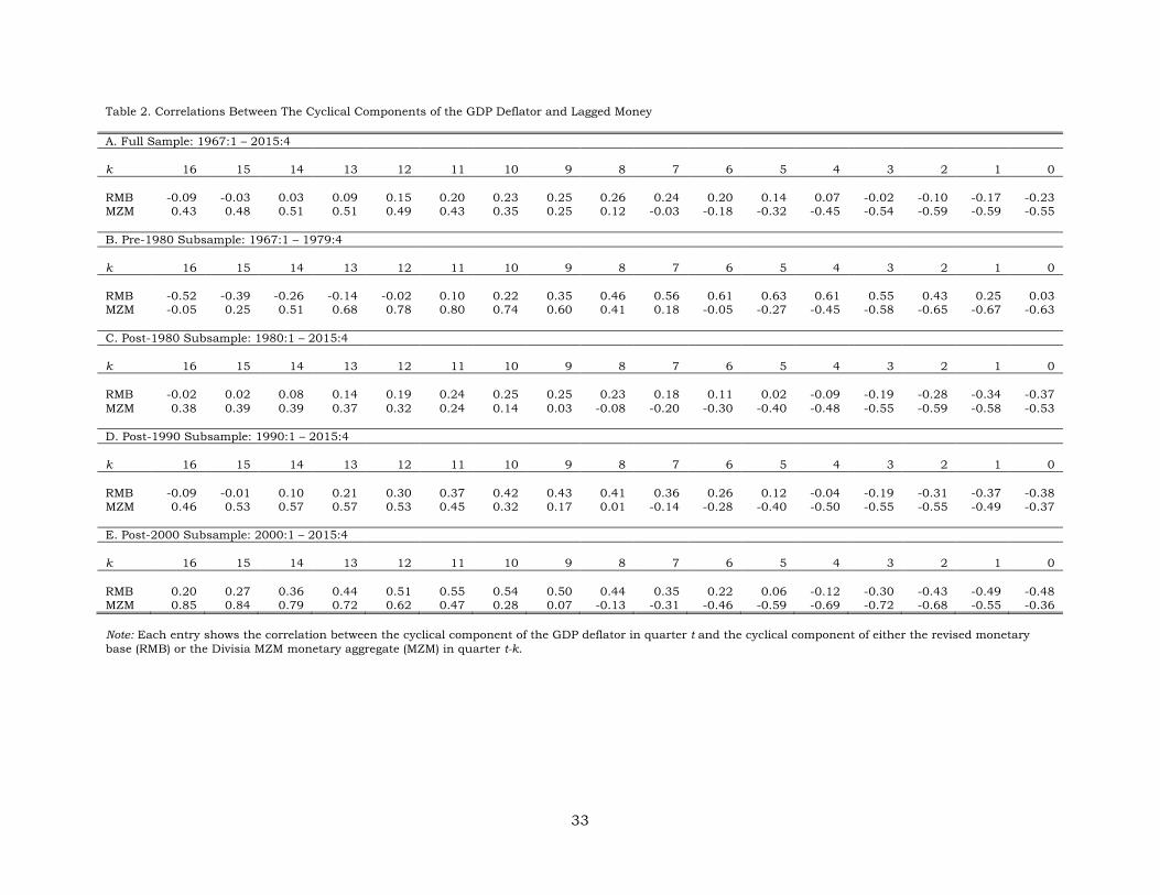
33

Table 2. Correlations Between The Cyclical Components of the GDP Deflator and Lagged Money A. Full Sample: 1967:1 – 2015:4 k 16 15 14 13 12 11 10 9 8 7 6 5 4 3 2 1 0 RMB -0.09 -0.03 0.03 0.09 0.15 0.20 0.23 0.25 0.26 0.24 0.20 0.14 0.07 -0.02 -0.10 -0.17 -0.23 MZM 0.43 0.48 0.51 0.51 0.49 0.43 0.35 0.25 0.12 -0.03 -0.18 -0.32 -0.45 -0.54 -0.59 -0.59 -0.55 B. Pre-1980 Subsample: 1967:1 – 1979:4 k 16 15 14 13 12 11 10 9 8 7 6 5 4 3 2 1 0 RMB -0.52 -0.39 -0.26 -0.14 -0.02 0.10 0.22 0.35 0.46 0.56 0.61 0.63 0.61 0.55 0.43 0.25 0.03 MZM -0.05 0.25 0.51 0.68 0.78 0.80 0.74 0.60 0.41 0.18 -0.05 -0.27 -0.45 -0.58 -0.65 -0.67 -0.63 C. Post-1980 Subsample: 1980:1 – 2015:4 k 16 15 14 13 12 11 10 9 8 7 6 5 4 3 2 1 0 RMB -0.02 0.02 0.08 0.14 0.19 0.24 0.25 0.25 0.23 0.18 0.11 0.02 -0.09 -0.19 -0.28 -0.34 -0.37 MZM 0.38 0.39 0.39 0.37 0.32 0.24 0.14 0.03 -0.08 -0.20 -0.30 -0.40 -0.48 -0.55 -0.59 -0.58 -0.53 D. Post-1990 Subsample: 1990:1 – 2015:4 k 16 15 14 13 12 11 10 9 8 7 6 5 4 3 2 1 0 RMB -0.09 -0.01 0.10 0.21 0.30 0.37 0.42 0.43 0.41 0.36 0.26 0.12 -0.04 -0.19 -0.31 -0.37 -0.38 MZM 0.46 0.53 0.57 0.57 0.53 0.45 0.32 0.17 0.01 -0.14 -0.28 -0.40 -0.50 -0.55 -0.55 -0.49 -0.37 E. Post-2000 Subsample: 2000:1 – 2015:4 k 16 15 14 13 12 11 10 9 8 7 6 5 4 3 2 1 0 RMB 0.20 0.27 0.36 0.44 0.51 0.55 0.54 0.50 0.44 0.35 0.22 0.06 -0.12 -0.30 -0.43 -0.49 -0.48 MZM 0.85 0.84 0.79 0.72 0.62 0.47 0.28 0.07 -0.13 -0.31 -0.46 -0.59 -0.69 -0.72 -0.68 -0.55 -0.36 Note: Each entry shows the correlation between the cyclical component of the GDP deflator in quarter t and the cyclical component of either the revised monetary base (RMB) or the Divisia MZM monetary aggregate (MZM) in quarter t-k.

34

Table 3. Estimated Forecasting Equations for Changes in Nominal GDP Growth Using the Revised Monetary Base Dependent variable: Change in nominal GDP growth (Δ2xt) Independent variables: Constant, four quarterly lags of changes in nominal GDP growth, and lagged nominal GDP gap (x*t-1 - xt-1) constructed with the revised monetary base A. Full Sample: 1967:1 – 2015:4 coefficient t stat (p value) constant -0.000 -0.789 (0.43) Δ2xt-1 -0.626 -8.951 (0.00) Δ2xt-2 -0.376 -4.734 (0.00) Δ2xt-3 -0.264 -3.319 (0.00) Δ2xt-4 -0.040 -0.576 (0.57) x*t-1 - xt-1 0.112 4.326 (0.00) 𝑅𝑅2 = 0.34 DW = 2.00 B. Pre-1980: 1967:1 – 1979:4 C. Post-1980: 1980:1 – 2015:4 coefficient t stat (p value) coefficient t stat (p value) constant 0.001 0.761 (0.45) -0.001 -1.020 (0.31) Δ2xt-1 -0.810 -5.318 (0.00) -0.502 -6.236 (0.00) Δ2xt-2 -0.569 -3.133 (0.00) -0.292 -3.312 (0.00) Δ2xt-3 -0.466 -2.608 (0.01) -0.159 -1.789 (0.08) Δ2xt-4 -0.125 -0.864 (0.39) -0.035 -0.432 (0.66) x*t-1 - xt-1 0.313 2.202 (0.03) 0.098 4.020 (0.00) 𝑅𝑅2 = 0.50 DW = 1.97 𝑅𝑅2 = 0.25 DW = 2.01 D. Post-1990: 1990:1 – 2015:4 E. Post-2000: 2000:1 – 2015:4 coefficient t stat (p value) coefficient t stat (p value) constant -0.000 -0.455 (0.65) -0.001 -0.907 (0.37) Δ2xt-1 -0.555 -5.788 (0.00) -0.578 -4.792 (0.00) Δ2xt-2 -0.283 -2.671 (0.01) -0.239 -1.766 (0.08) Δ2xt-3 -0.204 -1.903 (0.06) -0.091 -0.660 (0.51) Δ2xt-4 0.012 0.120 (0.90) 0.076 0.617 (0.54) x*t-1 - xt-1 0.067 3.068 (0.00) 0.091 3.196 (0.00) 𝑅𝑅2 = 0.28 DW = 1.96 𝑅𝑅2 = 0.30 DW = 1.94

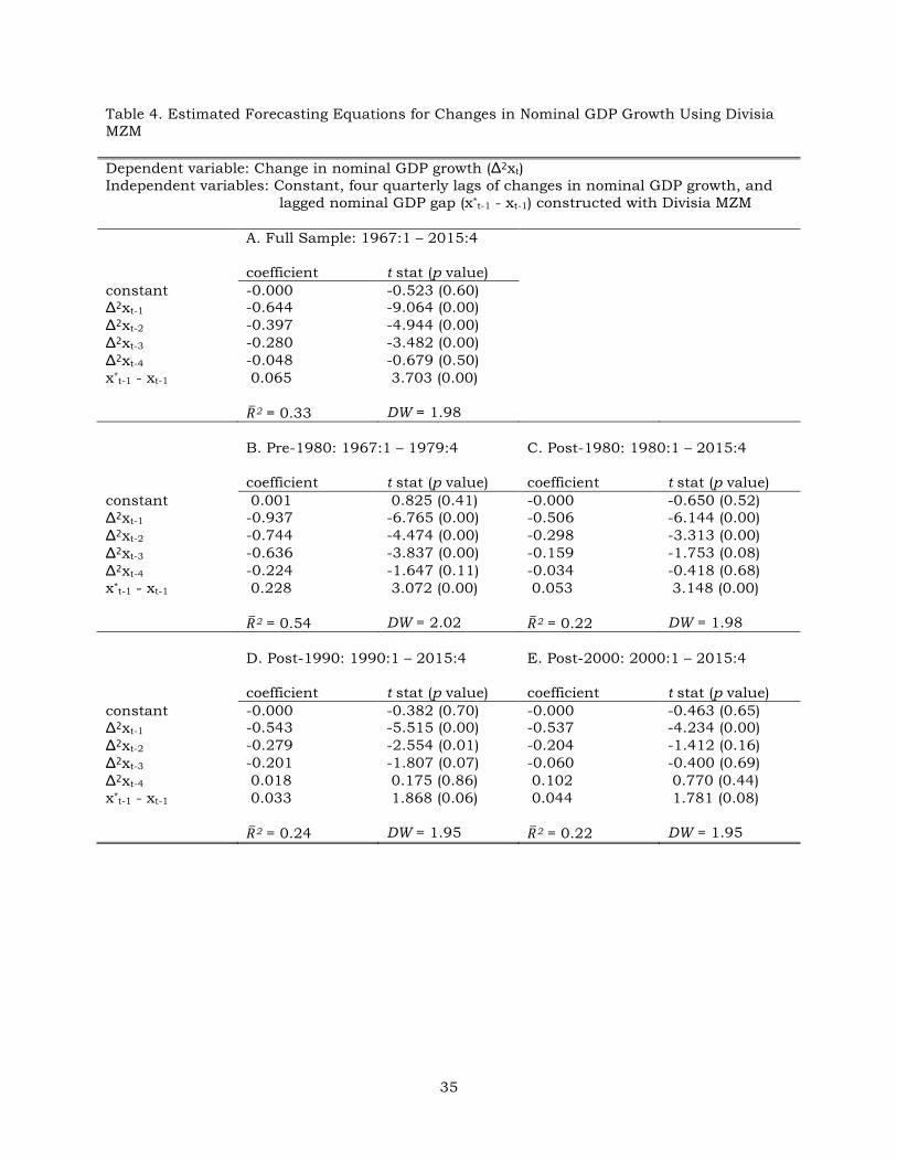
35

Table 4. Estimated Forecasting Equations for Changes in Nominal GDP Growth Using Divisia MZM Dependent variable: Change in nominal GDP growth (Δ2xt) Independent variables: Constant, four quarterly lags of changes in nominal GDP growth, and lagged nominal GDP gap (x*t-1 - xt-1) constructed with Divisia MZM A. Full Sample: 1967:1 – 2015:4 coefficient t stat (p value) constant -0.000 -0.523 (0.60) Δ2xt-1 -0.644 -9.064 (0.00) Δ2xt-2 -0.397 -4.944 (0.00) Δ2xt-3 -0.280 -3.482 (0.00) Δ2xt-4 -0.048 -0.679 (0.50) x*t-1 - xt-1 0.065 3.703 (0.00) 𝑅𝑅2 = 0.33 DW = 1.98 B. Pre-1980: 1967:1 – 1979:4 C. Post-1980: 1980:1 – 2015:4 coefficient t stat (p value) coefficient t stat (p value) constant 0.001 0.825 (0.41) -0.000 -0.650 (0.52) Δ2xt-1 -0.937 -6.765 (0.00) -0.506 -6.144 (0.00) Δ2xt-2 -0.744 -4.474 (0.00) -0.298 -3.313 (0.00) Δ2xt-3 -0.636 -3.837 (0.00) -0.159 -1.753 (0.08) Δ2xt-4 -0.224 -1.647 (0.11) -0.034 -0.418 (0.68) x*t-1 - xt-1 0.228 3.072 (0.00) 0.053 3.148 (0.00) 𝑅𝑅2 = 0.54 DW = 2.02 𝑅𝑅2 = 0.22 DW = 1.98 D. Post-1990: 1990:1 – 2015:4 E. Post-2000: 2000:1 – 2015:4 coefficient t stat (p value) coefficient t stat (p value) constant -0.000 -0.382 (0.70) -0.000 -0.463 (0.65) Δ2xt-1 -0.543 -5.515 (0.00) -0.537 -4.234 (0.00) Δ2xt-2 -0.279 -2.554 (0.01) -0.204 -1.412 (0.16) Δ2xt-3 -0.201 -1.807 (0.07) -0.060 -0.400 (0.69) Δ2xt-4 0.018 0.175 (0.86) 0.102 0.770 (0.44) x*t-1 - xt-1 0.033 1.868 (0.06) 0.044 1.781 (0.08) 𝑅𝑅2 = 0.24 DW = 1.95 𝑅𝑅2 = 0.22 DW = 1.95

36

Table 5. Estimated Forecasting Equations for Changes in GDP Price Inflation Using the Revised Monetary Base Dependent variable: Change in GDP price inflation (Δ2pt) Independent variables: Constant, four quarterly lags of changes in GDP price inflation, and lagged GDP price gap (p*t-1 - pt-1) constructed with the revised monetary base A. Full Sample: 1967:1 – 2015:4 coefficient t stat (p value) constant 0.000 1.168 (0.24) Δ2pt-1 -0.405 -5.635 (0.00) Δ2pt-2 -0.235 -3.065 (0.00) Δ2pt-3 -0.088 -1.142 (0.25) Δ2pt-4 0.116 1.616 (0.11) p*t-1 - pt-1 0.027 3.249 (0.00) 𝑅𝑅2 = 0.18 DW = 1.97 B. Pre-1980: 1967:1 – 1979:4 C. Post-1980: 1980:1 – 2015:4 coefficient t stat (p value) coefficient t stat (p value) constant 0.001 0.935 (0.36) 0.000 0.015 (0.99) Δ2pt-1 -0.464 -3.041 (0.00) -0.413 -4.923 (0.00) Δ2pt-2 -0.328 -2.008 (0.05) -0.231 -2.553 (0.01) Δ2pt-3 -0.225 -1.371 (0.18) -0.040 -0.438 (0.66) Δ2pt-4 0.072 0.466 (0.64) 0.098 1.178 (0.24) p*t-1 - pt-1 0.062 2.560 (0.01) 0.013 1.662 (0.10) 𝑅𝑅2 = 0.19 DW = 1.92 𝑅𝑅2 = 0.15 DW = 1.97 D. Post-1990: 1990:1 – 2015:4 E. Post-2000: 2000:1 – 2015:4 coefficient t stat (p value) coefficient t stat (p value) constant -0.000 -0.379 (0.71) -0.000 -0.081 (0.94) Δ2pt-1 -0.555 -5.509 (0.00) -0.544 -4.140 (0.00) Δ2pt-2 -0.390 -3.461 (0.00) -0.369 -2.463 (0.02) Δ2pt-3 -0.222 -1.931 (0.06) -0.226 -1.456 (0.15) Δ2pt-4 -0.053 -0.518 (0.61) -0.074 -0.543 (0.59) p*t-1 - pt-1 0.001 0.145 (0.89) 0.001 0.066 (0.95) 𝑅𝑅2 = 0.21 DW = 1.97 𝑅𝑅2 = 0.17 DW = 2.00

37

Table 6. Estimated Forecasting Equations for Changes in GDP Price Inflation Using Divisia MZM Dependent variable: Change in GDP price inflation (Δ2pt) Independent variables: Constant, four quarterly lags of changes in GDP price inflation, and lagged GDP price gap (p*t-1 - pt-1) constructed with Divisia MZM A. Full Sample: 1967:1 – 2015:4 coefficient t stat (p value) constant 0.000 0.334 (0.74) Δ2pt-1 -0.371 -5.138 (0.00) Δ2pt-2 -0.192 -2.498 (0.01) Δ2pt-3 -0.041 -0.533 (0.59) Δ2pt-4 0.160 2.219 (0.03) p*t-1 - pt-1 0.010 1.944 (0.05) 𝑅𝑅2 = 0.15 DW = 2.00 B. Pre-1980: 1967:1 – 1979:4 C. Post-1980: 1980:1 – 2015:4 coefficient t stat (p value) coefficient t stat (p value) constant 0.000 0.753 (0.46) -0.000 -0.670 (0.50) Δ2pt-1 -0.383 -2.573 (0.01) -0.404 -4.791 (0.00) Δ2pt-2 -0.204 -1.303 (0.20) -0.224 -2.457 (0.02) Δ2pt-3 -0.105 -0.667 (0.51) -0.029 -0.313 (0.75) Δ2pt-4 0.185 1.240 (0.22) 0.111 1.319 (0.19) p*t-1 - pt-1 0.046 2.142 (0.04) 0.004 0.821 (0.41) 𝑅𝑅2 = 0.15 DW = 2.05 𝑅𝑅2 = 0.14 DW = 1.97 D. Post-1990: 1990:1 – 2015:4 E. Post-2000: 2000:1 – 2015:4 coefficient t stat (p value) coefficient t stat (p value) constant -0.000 -1.100 (0.27) -0.000 -1.011 (0.32) Δ2pt-1 -0.580 -5.708 (0.00) -0.596 -4.496 (0.00) Δ2pt-2 -0.425 -3.731 (0.00) -0.444 -2.931 (0.00) Δ2pt-3 -0.256 -2.202 (0.03) -0.301 -1.924 (0.06) Δ2pt-4 -0.077 -0.749 (0.46) -0.120 -0.878 (0.38) p*t-1 - pt-1 -0.007 -1.233 (0.22) -0.013 -1.518 (0.13) 𝑅𝑅2 = 0.22 DW = 1.95 𝑅𝑅2 = 0.20 DW = 1.99

38

Figure 1. Monetary Growth and Velocity. The two top panels show year-over-year percentage changes in the revised monetary base and the Divisia MZM monetary aggregate, with shaded areas corresponding to NBER recession dates. The two bottom panels show the velocities of the revised monetary base and Divisia MZM (solid blue lines) together with their trend components (dotted red lines) computed with a one-sided Hodrick-Prescott filter.

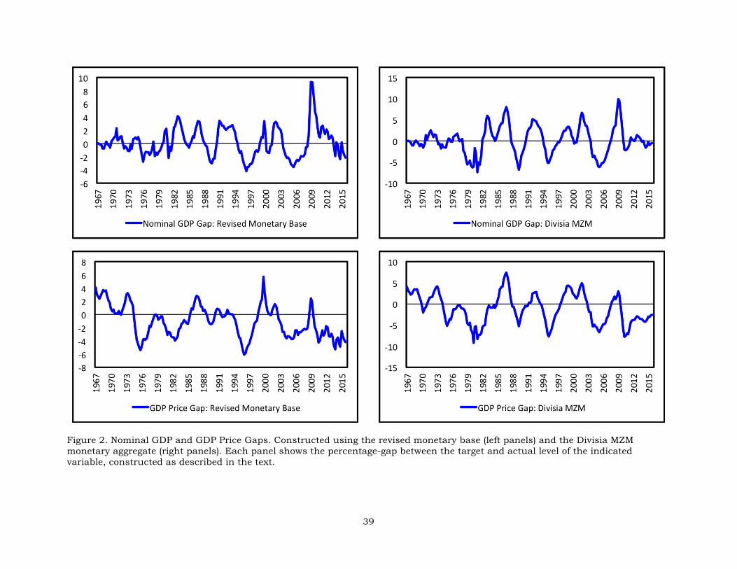
39

Figure 2. Nominal GDP and GDP Price Gaps. Constructed using the revised monetary base (left panels) and the Divisia MZM monetary aggregate (right panels). Each panel shows the percentage-gap between the target and actual level of the indicated variable, constructed as described in the text.

40

Figure 3. Nominal GDP and GDP Price Gaps and Growth Rates. Each panel compares the percentage-point gap between the target and actual level of the indicated variable (solid blue line) to the year-over-year growth rate in the actual value of the same variable (dotted red line).