Embed Size (px)
Citation preview

Chiral-scale Perturbation TheoryAbout an Infrared Fixed Point
Lewis C. Tunstallwith R.J. Crewther
Albert Einstein Centre for Fundamental PhysicsUniversitat Bern
13th International Conference on Meson-Nucleon Physics andthe Structure of the Nucleon, Rome, Italy, 30 September 2013

1 | QCD at low energies
Two powerful tools to analyse non-perturbative QCD
chiral symmetry
effective field theory [Weinberg 79]
Symmetry is hidden for 3 light quark flavours u, d , s
SU(3)L × SU(3)R −→ SU(3)V
〈qq〉vac 6= 0 most likely origin of chiral symmetry breaking
physical spectrum contains 8 pseudo-NG bosons {π,K , η}Model-independent marriage = chiral perturbation theory χPT3

1 | QCD at low energies
Two powerful tools to analyse non-perturbative QCD
chiral symmetry
effective field theory [Weinberg 79]
Symmetry is hidden for 3 light quark flavours u, d , s
SU(3)L × SU(3)R −→ SU(3)V
〈qq〉vac 6= 0 most likely origin of chiral symmetry breaking
physical spectrum contains 8 pseudo-NG bosons {π,K , η}
Model-independent marriage = chiral perturbation theory χPT3

1 | QCD at low energies
Two powerful tools to analyse non-perturbative QCD
chiral symmetry
effective field theory [Weinberg 79]
Symmetry is hidden for 3 light quark flavours u, d , s
SU(3)L × SU(3)R −→ SU(3)V
〈qq〉vac 6= 0 most likely origin of chiral symmetry breaking
physical spectrum contains 8 pseudo-NG bosons {π,K , η}Model-independent marriage = chiral perturbation theory χPT3

2 | QCD at low energies
trace anomaly associated with dilatations x → eξx
∂µDµ = θµµ =β(αs)
4αsG aµνG
aµν +(1 + γm(αs)
) ∑q=u,d ,s
mqqq
Gluonic anomaly −→ generates most of nucleon mass
MN = 〈N|θµµ|N〉 =β(αs)
4αs〈N|G a
µνGaµν |N〉+ O
(m2
K
)This talk
phenomenological implications for β → 0 in IR limit
extension of NG sector in 3-flavour theory
replacement of χPT3 with new effective field theory

2 | QCD at low energies
trace anomaly associated with dilatations x → eξx
∂µDµ = θµµ =β(αs)
4αsG aµνG
aµν +(1 + γm(αs)
) ∑q=u,d ,s
mqqq
Gluonic anomaly −→ generates most of nucleon mass
MN = 〈N|θµµ|N〉 =β(αs)
4αs〈N|G a
µνGaµν |N〉+ O
(m2
K
)
This talk
phenomenological implications for β → 0 in IR limit
extension of NG sector in 3-flavour theory
replacement of χPT3 with new effective field theory

2 | QCD at low energies
trace anomaly associated with dilatations x → eξx
∂µDµ = θµµ =β(αs)
4αsG aµνG
aµν +(1 + γm(αs)
) ∑q=u,d ,s
mqqq
Gluonic anomaly −→ generates most of nucleon mass
MN = 〈N|θµµ|N〉 =β(αs)
4αs〈N|G a
µνGaµν |N〉+ O
(m2
K
)This talk
phenomenological implications for β → 0 in IR limit
extension of NG sector in 3-flavour theory
replacement of χPT3 with new effective field theory

3 | Chiral SU(3)L × SU(3)R perturbation theory
χPT3
effective field theory for low-energy π,K , η interactions
well established tool to study non-perturbative QCD
Scattering amplitudes calculated via asymptotic series
A ={ALO +ANLO +ANNLO + . . .
}χPT3
powers of O(mK ) momentum and mu,d ,s = O(m2K )
Key premise —NG sector {π,K , η} dominates the non-NG sector {ρ, ω, . . .}PCAC = pole-dominance

4 | Problems with SU(3)L × SU(3)R?
Old observation — lowest order χPT3 fails for amplitudes with
a 0++ channel and O(mK ) extrapolations in momenta
Notable examplesFinal state ππ interactions important [Truong 84, 90]
K`4 decays [Truong 81]Non-leptonic K decays [Neveu & Scherk 70, Truong 88]Non-leptonic η decays [Roisnel 81, G & L 86, 96]
Γ(KL → π0γγ) only 1/3 measured value [Ecker et al. 87]
LO prediction for σ(γγ → π0π0) [Donoghue/Bijnens et al. 88]
February 1, 2008 8:4 WSPC/INSTRUCTION FILE review-mpla-rev
8 M.R. Pennington
Fig. 6. Integrated cross-section for γγ → ππ as a function of c.m. energy M(ππ) from Mark II 46, CrystalBall 47,48 and CLEO 49. The π0π0 results have been scaled to the same angular range as the charged data and byan isospin factor. Below are graphs describing the dominant dynamics in each kinematic region, as discussed inthe text.
Fig. 7. Cross-section for γγ → π0π0 integrated over | cos θ∗| ≤ 0.8 as a function of the ππ invariant mass M(ππ).The data are from Crystal Ball 47,48. The line is the prediction of χPT at one loop (1%) 53. The shaded bandshows the dispersive prediction 59,61,62 described later — its width reflects the uncertainties in experimentalknowledge of both ππ scattering and vector exchanges.
Figure: Pennington 07
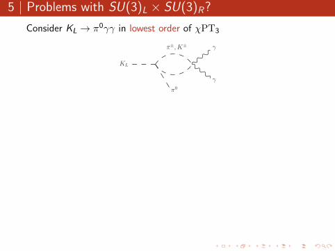
5 | Problems with SU(3)L × SU(3)R?
Consider KL → π0γγ in lowest order of χPT3
KL
π0
γ
γπ±, K±
Include dispersive NLO corrections and truncate series for A:
AKL→π0γγ '{ALO +ANLO
}χPT3
Fit to data achieved only for∣∣ANLO
∣∣χPT3
&√
2∣∣ALO
∣∣χPT3
Reconcile with success of χPT3 elsewhere?
Corrections to LO χPT3 should be ∼ 30% at most∣∣ANLO
/ALO
∣∣χPT3
. 0.3 , acceptable fit

6 | Problems with SU(3)L × SU(3)R?
Origin of large dispersive effects?
dispersive analysis of ππ-scattering + precise Ke4 dataindicates complex pole
√sp = M − iΓ/2 on second Riemann
sheet:
Mf0 = 441+16−8 MeV , Γf0 = 544+18
−25 MeV [Caprini et al. 06]
February 1, 2008 8:4 WSPC/INSTRUCTION FILE review-mpla-rev
4 M.R. Pennington
Fig. 2. An illustration of the sheets and cut structure of the complex energy plane in a world with just onethreshold and how these are connected. This represents the structure relevant to ππ scattering near its threshold.Experiment is performed on the top shaded sheet, just above the cut along the real energy axis. The cross on thelower, or second, sheet indicates where the σ-pole resides at E2 = s = sR. The ellipse above this on the top, orfirst, sheet indicates where the S -matrix is zero.
chiral constraints, allows the I = J = 0 ππ partial wave to be determined everywhere onthe first sheet of the energy plane 19, Fig. 2. As shown by Caprini et al. 17, this fixes azero of the S -matrix (symbolically depicted by the solid ellipse in Fig. 2) at E = 441 −i 227 MeV, which reflects a pole (denoted by the cross) on the second sheet at the sameposition. This not only confirms the σ as a state in the spectrum of hadrons but locatesthe position of its pole very precisely with errors of only tens of MeV. This is within theregion found by Zhou et al 20, who also took into account crossing and the left-hand cut.While the chiral expansion of amplitudes can have no poles at any finite order, particularsummations may. The inverse amplitude method 21 is one such procedure. Application ofthis by Pelaez et al. 22 did indeed find a pole in the same domain as Caprini et al. but manyyears earlier. However, without a proof that the Inverse Amplitude Method, rather thanany other, provided precision unitarisation of the low order chiral expansion, the presentauthor rather believed the analysis of a wide range of data of Ref. 10 that indicated nopole (or perhaps a very distant one). Now we know differently. There is a pole with awell-defined location. This is far from the position proposed by the treatment of Ishida etal. 23,24,25,26,27, the deficiencies of which were explained long ago in Ref. 21. (Bugg 28has added to these arguments in response to the discussion on the position of the κ by thesame group 29 .)
With a narrow resonance, there would naturally be a close correlation between the phasevariation of the underlying amplitude on the real axis and in the complex plane, as onepasses the pole. However, for the very short-lived σ, “deep” in the complex energy plane,this simple connection is lost. In Fig. 3 we show the phase of the I = J = 0 ππ → ππscattering amplitude along two lines in the complex energy plane. The phase along thereal axis is compared with relevant data from scattering 32 and Ke4 decays 6 in Fig. 3.One sees how different this phase is compared with that on the lower sheet of Fig. 2 atImE = −0.25 GeV. That deep in the complex plane shows the 180o phase change expectedof a resonance. It is the dramatic variation in the amplitude as one moves away from the
Figure: Pennington 07
Result is model-independent — derived from general principlesof QFT (Roy equations)

7 | Problems with SU(3)L × SU(3)R?
PDG have recently updated their entry for f0
Mf0 = (400− 550) MeV , Γf0 = (400− 700) MeV .
Dispersive techniques provide (in principle) controlled errorcalculation
Figure: Albaladejo and Oller 12

8 | Problems with SU(3)L × SU(3)R?
Conclude?
the existence of f0(500) well established
dispersion theory for K`4, nonleptonic K and η decays farbetter understood
But . . .
does not alter fact that LO of χPT3 fits these data so poorly
A ={ALO +ANLO +ANNLO + . . .
}χPT3
if first term poor fit −→ any truncation unsatisfactory
low energy expansion diverges

9 | Problems with SU(3)L × SU(3)R?
Two philosophies
limits to applicability of χPT3 — expect failures in a few cases
or
consistent trend of failure in 0++ channels which can andshould be corrected
Proposal: Modify lowest order of χPT3
Must preserve LO successes of χPT3 for reactions which donot involve f0(500) and O(mK ) extrapolations
spontaneously broken scale invariance identified as relevantsymmetry

10 | QCD Infrared fixed point
Scale invariance a generic feature at fixed points
∂µDµ = θµµ =β(αs)
4αsG aµνG
aµν +(1 + γm(αs)
) ∑q=u,d ,s
mqqq
O
β
αsαIR
Nf = 3 proposal
UV IR
Literature extensive, yet inconclusive on existence of αIR
lattice — no αIR for Nf < 8 [Appelquist et al. 09]
Dyson-Schwinger — αIR for Nf = 0, 3 [Alkofer, Fischer 97-03]
effective charges — ‘freezing’ [Mattingly & Stevenson 94, 13]
light-front holography — [Brodsky & de Teramond 10]

11 | f0(500) as a QCD dilaton
Gluonic anomaly absent at αIR −→ scale invariance
θµµ∣∣αs=αIR
=(1 + γm(αIR)
)(muuu + md dd + ms ss)
→ 0 , SU(3)L × SU(3)R limit
Conclude?
〈qq〉vac acts as both a chiral and scale condensate
NG sector extended to include 0++ dilaton σ = f0
{π,K , η} −→ {π,K , η, σ/f0}
replace χPT3 −→ chiral-scale perturbation theory χPTσ
in χPTσ, ms sets scale of m2f0
as well as m2K and m2
η
PCDC = σ-pole dominance in 0+ channels

12 | Separation of scales
χPT2
χPT3
NG bosons
p·p′=O(m2π) Not NG bosons
π f0 K η(mass)2
0
0
χPTσ
(mass)2
(mass)2
π
f0
K η
ρ
π f0 K η ρ
Not NG bosons0
0
NG bosons p·p′=O(m2K)
NG bosons p·p′=O(m2K)
(mass)2
Not NGbosons
scaleseparation
scaleseparation
rules for counting powers of mK changed in χPTσ— f0 pole amplitudes promoted to LO

13 | Infrared expansions
both χPT3 and χPTσ involve the limit
mi ∼ 0 , mi/mj fixed, i , j = u, d , s
amplitudes expanded in powers and logs of
{momenta}/χch � 1 , χch ≈ 1 GeV
χch ' 4πFπ in χPT3 (‘dim. analysis’) [Manohar & Georgi 84]
chiral scale χch also sets mass scale for non-NG particles

13 | Infrared expansions
both χPT3 and χPTσ involve the limit
mi ∼ 0 , mi/mj fixed, i , j = u, d , s
amplitudes expanded in powers and logs of
{momenta}/χch � 1 , χch ≈ 1 GeV
χch ' 4πFπ in χPT3 (‘dim. analysis’) [Manohar & Georgi 84]
chiral scale χch also sets mass scale for non-NG particles

13 | Infrared expansions
both χPT3 and χPTσ involve the limit
mi ∼ 0 , mi/mj fixed, i , j = u, d , s
amplitudes expanded in powers and logs of
{momenta}/χch � 1 , χch ≈ 1 GeV
χch ' 4πFπ in χPT3 (‘dim. analysis’) [Manohar & Georgi 84]
chiral scale χch also sets mass scale for non-NG particles

13 | Infrared expansions
both χPT3 and χPTσ involve the limit
mi ∼ 0 , mi/mj fixed, i , j = u, d , s
amplitudes expanded in powers and logs of
{momenta}/χch � 1 , χch ≈ 1 GeV
χch ' 4πFπ in χPT3 (‘dim. analysis’) [Manohar & Georgi 84]
chiral scale χch also sets mass scale for non-NG particles

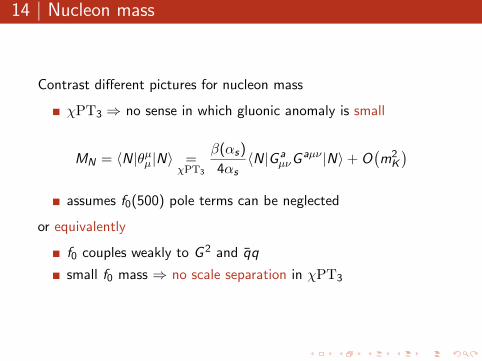
14 | Nucleon mass
Contrast different pictures for nucleon mass
χPT3 ⇒ no sense in which gluonic anomaly is small
MN = 〈N|θµµ|N〉 =χPT3
β(αs)
4αs〈N|G a
µνGaµν |N〉+ O
(m2
K
)assumes f0(500) pole terms can be neglected
or equivalently
f0 couples weakly to G 2 and qq
small f0 mass ⇒ no scale separation in χPT3

14 | Nucleon mass
Contrast different pictures for nucleon mass
χPT3 ⇒ no sense in which gluonic anomaly is small
MN = 〈N|θµµ|N〉 =χPT3
β(αs)
4αs〈N|G a
µνGaµν |N〉+ O
(m2
K
)
assumes f0(500) pole terms can be neglected
or equivalently
f0 couples weakly to G 2 and qq
small f0 mass ⇒ no scale separation in χPT3

14 | Nucleon mass
Contrast different pictures for nucleon mass
χPT3 ⇒ no sense in which gluonic anomaly is small
MN = 〈N|θµµ|N〉 =χPT3
β(αs)
4αs〈N|G a
µνGaµν |N〉+ O
(m2
K
)assumes f0(500) pole terms can be neglected
or equivalently
f0 couples weakly to G 2 and qq
small f0 mass ⇒ no scale separation in χPT3

15 | Nucleon mass
In χPTσ
infrared regime emphasizes values of αs close to αIR
O
β
αsαIR
Nf = 3 proposal
UV IR
combined limit must be considered
mu,d ,s ∼ 0 and αs . αIR
β(αs) small ⇒ gluonic anomaly small as an operator
but can produce large amplitudes when coupled to dilatons

15 | Nucleon mass
In χPTσ
infrared regime emphasizes values of αs close to αIR
O
β
αsαIR
Nf = 3 proposal
UV IR
combined limit must be considered
mu,d ,s ∼ 0 and αs . αIR
β(αs) small ⇒ gluonic anomaly small as an operator
but can produce large amplitudes when coupled to dilatons

15 | Nucleon mass
In χPTσ
infrared regime emphasizes values of αs close to αIR
O
β
αsαIR
Nf = 3 proposal
UV IR
combined limit must be considered
mu,d ,s ∼ 0 and αs . αIR
β(αs) small ⇒ gluonic anomaly small as an operator
but can produce large amplitudes when coupled to dilatons

15 | Nucleon mass
In χPTσ
infrared regime emphasizes values of αs close to αIR
O
β
αsαIR
Nf = 3 proposal
UV IR
combined limit must be considered
mu,d ,s ∼ 0 and αs . αIR
β(αs) small ⇒ gluonic anomaly small as an operator
but can produce large amplitudes when coupled to dilatons

16 | Nucleon mass
θµµ
N N
σ
gσNN
σ couples to vacuum via divergence of symmetry current
〈σ|θµµ|vac〉 = −m2σFσ = O(m2
σ) , mσ → 0
nucleon mass remains massive in scaling limit
analogue of Goldberger-Treiman relation
FσgσNN ' MN
analysis of NN scattering: gσNN ' 9 [Calle-Cordon et al. 08]
Fσ ≈ 100 MeV cf. Fπ ' 93 MeV

17 | Nucleon mass
In χPTσ
gluonic anomaly and the quark mass term in for θµµ cancontribute to MN in the chiral-scale limit
NG boson requirement
m2σ = O(m2
K ) = O(mu,d ,s)
Allows the constants FG2 and Fqq given by
β(αs)/
(4αs)〈σ|G 2|vac〉 = −m2σFG2 ,
{1 + γm(αs)}∑
q=u,d ,s
mq〈σ|qq|vac〉 = −m2σFqq
to remain finite in chiral-scale limit θµµ → 0
MN ' FG2gσNN + FqqgσNN

18 | Chiral-Scale Lagrangian
Consider physical region 0 < αs < αIR
L[σ,U,U†
]= Ld=4
inv + Ld>4anom + Ld<4
mass
Building blocks
chiral invariant QCD dilaton σ
SU(3) field U = U(π,K , η)
Operator dimensions satisfy
dinv = 4 and 1 6 dmass < 4 [Wilson 69]
Callan-Symanzik equation for QCD amplitudes
dmass = 3− γm(αIR
)and danom = 4 + β′
(αIR
)> 4
consistency requires Lanom = O(∂2,M)

19 | Chiral-Scale Lagrangian
Want formula for L[σ,U,U†
]= Ld=4
inv + Ld>4anom + Ld<4
mass
dilaton transforms non-linearly
σ → σ − 14Fσ log
∣∣ det(∂x ′/∂x)∣∣
d = 1 building block for scale symmetry: eσ/Fσ
K[U,U†
]= 1
4F2πTr(∂µU∂
µU†) Kσ =1
2∂µσ∂
µσ
at lowest order in χPTσ
Ld=4inv =
{c1K + c2Kσ + c3e
2σ/Fσ}e2σ/Fσ
Ld>4anom =
{(1− c1)K + (1− c2)Kσ + c4e
2σ/Fσ}e(2+β′)σ/Fσ
Ld<4mass = Tr(MU† + UM†)e(3−γm)σ/Fσ
vacuum stability −→ c3,4 ∼ O(M)

20 | Strong interactions
From L obtain dilaton mass
m2σF
2σ = F 2
π (m2K + 1
2m2π)(3− γm)(1 + γm)− β′(4 + β′)c4] ,
and the effective σππ coupling
Lσππ ={(
2 + (1− c1)β′)|∂π|2 − (3− γm)m2
π|π|2}σ/(2Fσ)
Key feature: mostly derivative
small effect on ππ-scattering in SU(2)L × SU(2)R limit∂ = O(mπ)
vertex for on-shell amplitude for σ → ππ:
gσππ = −(2 + (1− c1)β′
)m2σ/(2Fσ) + O(m2
π)

21 | χPTσ at next to leading order
Add σ-loops to χPT3 analysis to test convergence of χPTσ
involves unknown LECs β′, γ, c1...4 in σσσ and σσππ vertices
π
ππ
π
π, Kσ
Apply Manohar & Georgi to first diagram
Aloop
/Atree ∼
1
16π2F 2π
× logarithms
in χPTσ must add ∼{
1
16π2F 2σ
andF 2π
16π2F 4σ
}× logarithms
in principle two χPTσ scales
χπ = 4πFπ and χσ = 4πFσ ; χπ ≈ χσ ≈ 1 GeV

22 | The f0 width in χPTσ
The f0(500) is almost as broad as it is heavy
is Γσ a LO effect?
invalidates PCDC?
Estimate width a la Manohar & Georgi
Γσππ ≈|gσππ|216πmσ
∼ m3σ
16πF 2σ
∼ 250 MeV
justified use of tree approximation to generate LO of χPTσ
methods like complex mass scheme may be necessary beyondLO and in degenerate cases KL − KS oscillations

23 | Weak interactions
In the leading order of χPT3
Lweak|χPT3= g8Q8 + g27Q27 + Qmw + h.c.
vacuum stability? [Crewther 86]
Qmw = Tr(λ6 − iλ7)(gMMU† + gMUM†
)absorbed by field rotation −→ cannot be used to explain∆I = 1/2 rule
in χPTσ, anomalous mass dimensions unrelated
3− γm(αIR) 6= 3− γmw (αIR)
Qmweσ(3−γmw )/Fσ cannot be eliminated by chiral rotation

24 | Weak interactions
scale weak operators and align vacuum
Lalignweak =Q8
∑n
g8ne(2−γ8n)σ/Fσ + g27Q27e
(2−γ27)σ/Fσ
+ Qmw
{e(3−γmw )σ/Fσ − e(3−γm)σ/Fσ
}+ h.c.
residual interaction mixes KS and σ in leading order
gKσ = (γm − γmw )<e[(2m2K −m2
π)gM −m2πgM ]Fπ/Fσ
produces a pure ∆I = 1/2 amplitude
+K0S
π
π
g8,27
σ
gσππgKSσ

25 | Weak interactions
key processes: KS → γγ and γγ → ππ
|gKσ| ≈ 4.4× 10³ keV2, 30% precision
to the extent that gσNN and hence Fσ can be determined
|Aσ-pole| ≈ 0.34 keV cf. data |A0|expt. = 0.33 keV
conclude g8 =∑
n g8n and g27 can have similar magnitudes
leading order of χPTσ explains the ∆I = 1/2 puzzle

Electromagnetic interactions
electromagnetic anomaly [Crewther 72; Chanowitz & Ellis 72]
θµµ∣∣strong + e′mag
= θµµ + (Rα/6π)FµνFµν ,
R =σ(e+e− → hadrons)
σ(e+e− → µ+µ−)
∣∣∣∣high−energy
anomaly realised in χPTσ through effective coupling
Lσγγ = 12gσγγσFµνF
µν , gσγγ =(RIR − 1
2 )α
3πFσ
dispersive methods determine f0 → γγ width [Pennington 06]
Γf0γγ = 1.98± 0.3 keV [Oller & Roca 08]
non-perturbative χPTσ prediction RIR ≈ 5

Concluding remarks
The assumption of aninfrared fixed point in3-flavour QCD leads to anextended Goldstone sector{π,K , η, σ}, where σ isidentified with f0(500) as theNG-boson of spontaneouslybroken scale symmetry.
O
β
αsαIR
Nf = 3 proposal
UV IR
Model independent theory χPTσ promotes f0 pole terms toleading order ⇒ χPT3’s problems in the 0++ channelovercome.
Retains χPT3’s successful predictions elsewhere: NLOanalysis of strong sector in progress.
The ∆I = 1/2 rule for K -decays emerges as a consequence ofχPTσ.
χPTσ has implications for CP violation, rare kaon decays, andpossibly η → 3π.
![On-Shell Approach to Pion-Nucleon Physics · 2017. 11. 3. · The scattering amplitude is analytically continued to the unphysical Cheng-Dashen point [3], and chiral perturbation](https://img.dokumen.tips/doc/110x75/60eeca471db474481320e2d2/on-shell-approach-to-pion-nucleon-physics-2017-11-3-the-scattering-amplitude.jpg)


![Chiral Perturbation Theory for Lattice QCDinspirehep.net/record/1338236/files/baer.pdf · [5] Chiral perturbation theory for staggered sea quarks and Ginsparg-Wilsonvalencequarks,](https://img.dokumen.tips/doc/110x75/5e6d7176f30da1321d183fb3/chiral-perturbation-theory-for-lattice-5-chiral-perturbation-theory-for-staggered.jpg)