D e p a r t m e n t o f A p p l i e d C h e m i s t r y

Supervisor : Dr. Kriveshini Pillay Co-Supervisor : Dr. Arjun Maity Dr. Sushanta Debnath Dr. Niladri Ballav

Slide 2

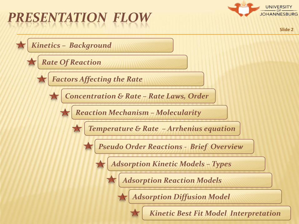
PRESENTATION FLOW

Kinetics – Background

Rate Of Reaction

Factors Affecting the Rate

Concentration & Rate – Rate Laws, Order

Reaction Mechanism – Molecularity

Pseudo Order Reactions - Brief Overview

Adsorption Kinetic Models – Types

Adsorption Reaction Models

Adsorption Diffusion Model

Temperature & Rate – Arrhenius equation

Kinetic Best Fit Model Interpretation

KINETICS - BACKGROUND

Slide 3

• To understand & predict behaviour of a chemical system one must consider both Thermodynamics & Kinetics

• Factors to be considered when predicting whether or not a change will take place

Thermodynamics : does a reaction takes place ???

Kinetics : how fast does a reaction proceed ???

1. Gibbs Free Energy ΔG

2. Entropy Change ΔS

3. The RATE of the change

Thermodynamics

Kinetics

RATE OF REACTION Slide 4

Change in the concentrations of reactants or products per unit time Progress of a simple reaction, • Concentration of Reactant A

(purple ) decreases with time

• Concentration of Product B

( Green ) increases with time

• Concentrations of A & B are measured at time t1 & t2 respectively A1 , A2 & B1 , B2

Reactant A Product B

The graph shows the change in the number of A and B molecules in the reaction as a function of time over a 1 min period (bottom)

Rate Of Reaction

CONTINUED ....... Slide 5

Δ[A]

Δt Rate = Change in concentration of A

change in time

Conc. A2 – Conc. A1

t2 - t1 = - = -

Δ[B] Δt

Rate = Change in concentration of B

change in time

Conc. B2 – Conc. B1

t2 - t1 = =

Rate = = ................................ for simpler reactions

The ( - ve ) sign is used because the concentration of A is decreasing.

Δ[A] Δt

Δ[B] Δt

Rate with respect to A

Rate with respect to B

CONTINUED ..... Slide 6

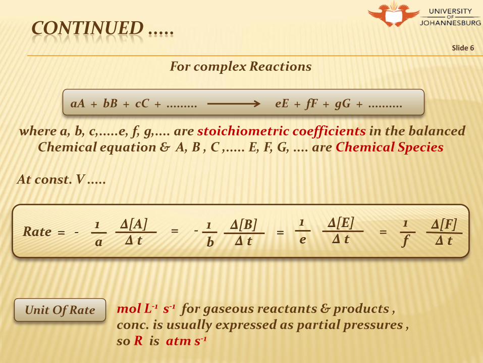
For complex Reactions

where a, b, c,.....e, f, g,.... are stoichiometric coefficients in the balanced Chemical equation & A, B , C ,..... E, F, G, .... are Chemical Species

At const. V .....

mol L-1 s-1 for gaseous reactants & products , conc. is usually expressed as partial pressures , so R is atm s-1

1

a

∆[A] ∆ t

1

b

∆[B] ∆ t

Rate = - = - 1

e ∆[E] ∆ t

= 1

f ∆[F] ∆ t

=

aA + bB + cC + ......... eE + fF + gG + ..........

Unit Of Rate

CONTINUED ..... Slide 7

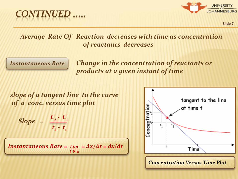
Average Rate Of Reaction decreases with time as concentration of reactants decreases

Change in the concentration of reactants or products at a given instant of time

slope of a tangent line to the curve of a conc. versus time plot

Slope = C2 - C1

t2 - t1

Instantaneous Rate = Lim = Δx/Δt = dx/dt t 0

Concentration Versus Time Plot

Instantaneous Rate

FACTORS AFFECTING THE RATE Slide 8

Nature Of Reactants

Concentration Of Reactants

Temperature

Surface Area Of Reactants

Catalyst

F A C T O R S

The same mass of Steel wool bursts into flame

A Hot Steel nail glows feebly when placed in oxygen

• • Heterogeneous reaction occurs at interface of two phases of reactants • If one reactant is Solid , rate increases with increase in surface area of solid phase reactant • Surface area increases , area of contact between reactants increases - rate of encounter between reactants increases - Rate increases • Surface area of a solid can be increased by Sub-division i.e. dividing the bigger particles in smaller

Surface Area Of Reactants

• Rate of “ Homogeneous Reactions” is higher than the “Heterogeneous Reactions” • Rate depends on the physical state of reactants , e.g. liquid /gaseous/solid • Rate depends on the number of collisions or encounters between the reacting species

Nature Of Reactants

CONTINUED...... Slide 9

V = 1 m3 A = 6 m2

V = 1 m3 A = 8 m2

V = 1 m3 A = 12 m2

V = 1 m3 A = 36 m2

V = 1 m3 A = 20 m2

V = 1 m3 A = ?????

CONCENTRATION & TEMPERATURE

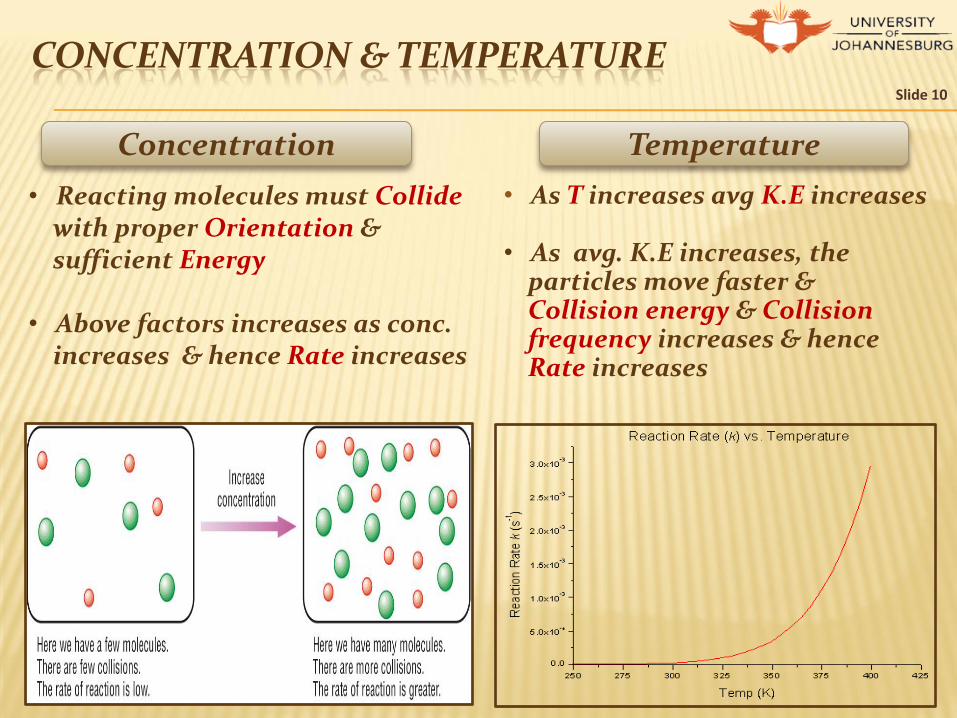
Concentration Temperature

• Reacting molecules must Collide with proper Orientation & sufficient Energy • Above factors increases as conc. increases & hence Rate increases

• As T increases avg K.E increases • As avg. K.E increases, the particles move faster & Collision energy & Collision frequency increases & hence Rate increases

Slide 10

PRESENCE OR ABSENCE OF CATALYST

Catalyst

• A substance that increases the reaction rate without undergoing a chemical change itself • Provides an alternate reaction mechanism faster than mechanism in absence of catalyst • Lowers the activation energy for a chemical reaction • Simple Catalyzed Reaction Scheme : C is catalyst , R1 & R2 reactants , P1 &

P2 products , I is intermediate I + R2 I + P2

R1 + C I + P1

Slide 11

CONCENTRATION & RATE Slide

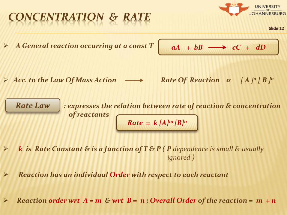
A General reaction occurring at a const T

Acc. to the Law Of Mass Action Rate Of Reaction α [ A ]a [ B ]b : expresses the relation between rate of reaction & concentration of reactants k is Rate Constant & is a function of T & P ( P dependence is small & usually ignored ) Reaction has an individual Order with respect to each reactant

Reaction order wrt A = m & wrt B = n ; Overall Order of the reaction = m + n

aA + bB cC + dD

Rate Law

Rate = k [A]m [B]n

Slide 12

CONTINUED ...... Slide 13

[A] versus Time plot for 0, 1st & 2nd order rxns Rate versus [A] plot for 0, 1st , 2nd order rxns

Reaction Order “n”

Rate variation with Conc.

Differential Rate Law

Integrated Rate Law

1

Rate doubles when [A] doubles

Rate = k [A]1

ln [A]t /[A]o = -kt

2

Rate quadruples as [A] doubles

Rate = k [A]2

1/[ A]t = kt + 1/[A]0

0

Rate does not change with [A]

Rate = k [A]0

[A]t - [A]0 = - kt

A Products

CONTINUED ...... Slide 14

2NO(g) + 2H2(g) N2(g) + 2H2O(g)

Rate Law : k[NO]2[H2] Order of reaction = 3

1st Order wrt [H2 ]

2nd Order wrt [ NO]

Stoichiometric coefficient of [H2] = 2

Order with respect to [H2] = 1

Reaction orders must be determined from experimental data and cannot be deduced from the balanced equation

Method for determining Order of reaction

Half Life Method

Powell Plot Method

Isolation Method

Initial Rate Method

CONTINUED ...... Slide 15

Initial Rate Method

Information sequence to determine the Kinetic parameters of a Reaction

Rate Constant k & actual rate

law

Calculation of Reaction order

Initial rates determination by

drawing tangent to the plot of Conc vs T

Series of Plot of Concentration

versus time

• A series of experiments wherein the concn of one reactant at a time is varied, initial rate R0 at time t0 of the rxn is measured. • By comparing the conc. change to the Rate change, Order wrt each reactant can be determined

REACTION MECHANISM Slide 16

Reactions can be divided on the basis of Reaction mechanism

Elementary Reactions Complex Reactions

• Only one step reactions • No Intermediate • Only One Transition state • Further divided in Unimolecular , Bimolecular & Termolecular rxn based on Molecularity

• Two or more steps • With Intermediate formation • Multiple Transition states • Rate of over all complex rxn is the rate of slowest rxn step (Rate determining Step)

Complex Reaction Elementary Reaction

MOLECULARITY Slide 17

Number of colliding molecular entities that are involved in a single reaction step

Molecularity

Unimolecular Termolecular Bimolecular

Molecularity Examples Rate law Elementary Step

Unimolecular

Bimolecular

Termolecular

A Products

A + A Products A + B Products A + A + A Products A + A + B Products A + B + C Products

rate=k [A]

rate=k[A]2

rate=k [A][B]

rate=k[A][B] rate=k[A][B]

rate=k[A]3 rate=k [A]2 [B]

rate = k [A][B][C]

N2O4(g)→2NO2(g)

2NOCl→2NO(g)+CO2(g) CO(g)+NO3(g)→NO2(g)+CO2(g)

2NO(g)+O2(g)→2NO2(g) H+O2(g)+M→HO2(g)+M

CONTINUED ...... Slide 18

Molecularity

• Number of reacting species which collide to result in reaction • Only positive integral values e.g 1,2,3 & never –ve • Theoretical concept & value is derived from mechanism of reaction

• Sum of powers to which concentrations are raised in the rate law expression • Zero, fractional or even be -ve • Experimental fact & derived from rate law

Slowest step of a chemical reaction

that determines the speed (rate) at

which the overall reaction proceeds

Rate Determining

Step

Eg : A complex reaction

NO2(g)+CO(g)→NO(g)+CO2(g) occur in two elementary steps : NO2+NO2→NO+NO3 (slow) rate const k1 NO3+CO→NO2+CO2 (fast) rate const k2

Rate= k1 [NO2][NO2] = k1 [NO2]2

Order

TEMPERATURE & RATE Slide 19

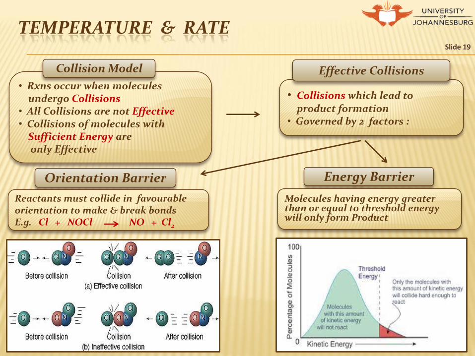
• Rxns occur when molecules undergo Collisions • All Collisions are not Effective • Collisions of molecules with Sufficient Energy are only Effective

Collision Model

• Collisions which lead to product formation • Governed by 2 factors :

Effective Collisions

Energy Barrier

Molecules having energy greater than or equal to threshold energy will only form Product

Orientation Barrier Reactants must collide in favourable orientation to make & break bonds E.g. Cl + NOCl NO + Cl2

CONTINUED ... Slide 20

Increase in temperature increases the no. of Effective collisions i.e fraction of colliding molecules that have enough energy to exceed Ea

increases

Explanation for increase in Rate of reaction with temperature by : Energy- distribution Curve at two temperatures T2 & T1

Taking log

ln k = ln A - Ea / RT

CONTINUED ..... Slide 21

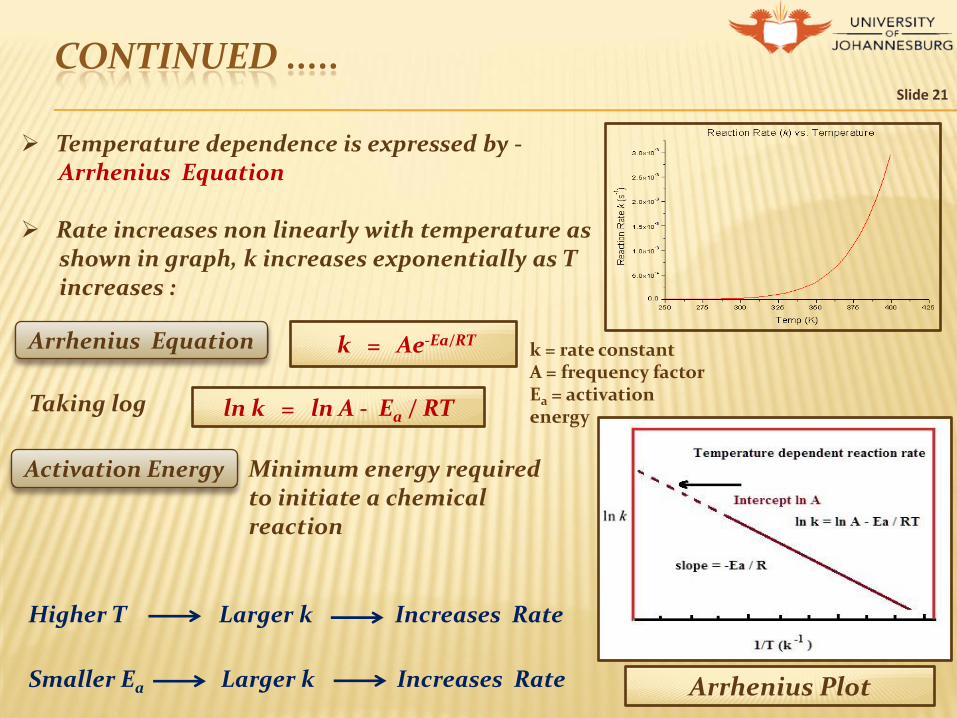
Temperature dependence is expressed by - Arrhenius Equation Rate increases non linearly with temperature as shown in graph, k increases exponentially as T increases :

k = Ae-Ea/RT Arrhenius Equation k = rate constant A = frequency factor Ea = activation energy

Arrhenius Plot

Minimum energy required to initiate a chemical reaction

Activation Energy

Higher T Larger k Increases Rate

Smaller Ea Larger k Increases Rate

PSEUDO ORDER REACTIONS Slide 22

An order of a chemical reaction that appears to be less than the true order due to experimental conditions ; when one reactant is in large excess

Pseudo Order Reactions

Pseudo Second Order Reactions

Pseudo First Order Reactions

2nd Order kinetics can be approximated as 1st Order under certain experimental condition

3rd Order kinetics can be approximated as 2nd Order under certain experimental condition

Pseudo first order kinetics 2nd order rate law = k [A] [B] • Reduces to Pseudo first order if either [A] or [B] is in large excess • Pseudo first order rate law = k’ [B] where k’ = k [A] ...... Pseudo first order rate constant

Pseudo Second order kinetics 3rd order rate law = k [A]2 [B] • Reduces to Pseudo first order , if [A] is in excess Pseudo second order if [B] is in excess • Pseudo Second order rate law = k’ [A]2 where k’ = k [B] ...... Pseudo second order rate constant

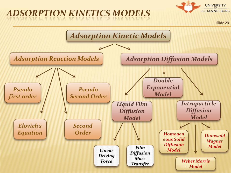
ADSORPTION KINETICS MODELS Slide 23

Adsorption Kinetic Models

Adsorption Diffusion Models Adsorption Reaction Models

Pseudo first order

Elovich’s Equation

Second Order

Pseudo Second Order

Intraparticle Diffusion

Model

Liquid Film Diffusion

Model

Film Diffusion

Mass Transfer

Linear Driving

Force

Homogeneous Solid Diffusion

Model

Weber Morris Model

Dumwald Wagner Model

Double Exponential

Model

ADSORPTION REACTION MODELS Slide 24

Pseudo First Order

• Earliest Model ; Proposed by Lagergren (1898) to describe kinetic process of Liq-sol phase adsorption

• Recent uses : kinetic study of adsorption of pollutants from waste water

dqt / dt = kp1 ( qe – qt )

Rate Equation

log (qe – qt ) = log qe - kp1 t /2.303 • Integrated form of rate eq.

• Plot of log (qe – qt ) ~ t should give a linear relationship Lagergren Plot ; kp1

& qe can be determined from slope & intercept of Lagergren Plot

• Fig 1 : Lagergren Plot for Cadmium adsorption on Rice husk

Fig 1

ADSORPTION REACTION MODELS Slide 25

Pseudo Second Order

• Proposed by Ho (1995) • To describe kinetic process of adsorption of divalent metal ions on Peat • Recent Uses : Kinetic study of adsorption process of divalent metal ions, dyes , organic substances from aq. solns

d (P)t / dt = kp2 [(P)0 - (P)t]2 Rate Equation

t/ qt = 1/ kp2 q2

e + 1/ qe t • Integrated form of rate eq.

• Plot of t/ qt ~ t should give a linear relationship with a slope of 1/ qe &

intercept of 1/ kp2 q2

e • Fig 2 : Pseudo second order plot for Pb2+ ions onto NSSCAC at diff concs.

Fig 2

ADSORPTION REACTION MODELS Slide 26

Elovich’s Model

• Proposed by Zeldowitsch (1934) to study kinetics of Chemisorption of gases onto heterogeneous solids

• Recent Uses : kinetics study of removal of pollutants from aq. solns

dq /dt = ae-αq

Elovich Equation

q = αln (aα) + αlnt • Integrated form of rate eq.

• Plot of q ~ lnt should be linear Elovich Plot ; slope gives α & intercept gives a

• Fig 3 : Elovich Plot for uptake of Cu(II) from copper solns at two concs 10mg/L & 100mg/L

Fig 3

LIQUID FILM DIFFUSION MODEL Slide 27

Liquid Film Diffusion Model

δq /δt = kf S0(C – Ci ). ln ( 1- qt/qe ) = - 3D1

et/r0Δr0k’

Linear driving force rate law Film Diffusion Mass transfer rate law

2 Rate laws of this model

• Applied to describe mass transfer through liquid film

• Plot of ln ( 1- qt/qe ) ~ t straight line

with a slope of 3D1e/r0Δr0k if the

film diffusion is the rate limiting step • Recent Uses : Applied to model several liquid / solid adsorption cases e.g. Phenol adsorption by a polyemric adsorbent NDA – 100 • Fig 4 : Liquid film diffusion model plot

Fig 4

INTRAPARTICLE DIFFUSION MODEL Slide 28

Intraparticle Diffusion Model

Homogeneous Solid diffusion Model Webber Morris model

3 types of Intraparticle diffusion model

Dumwald - Wagner model

Homogeneous Solid diffusion Model

• Describes mass transfer in an amorphous & homogeneous sphere

δq /δt = Ds /r2 δ/δr (r2 δq/δr)

HSDM Equation

• Recent Uses : Kinetic study of adsorption of salicylic acid & 5- sulfosalicylic acid from aq. solns by hypercrosslinked polymeric adsorbent NDA-99 & NDA - 101

Ds = intraparticle

diffusion coefficient

r = radial position

q = adsorption quantity of

solute in the solid varying with radial position at

time t

CONTINUED..... Slide 29

qt = kint t1/2 + Ci

• Plot of qt ~ t1/2 should be straight line with a slope of kint & intercept Ci = 0 when Intraparticle diffusion is the rate limiting step

Webber Morris model

• Acc to this model : solute uptake varies proportionally with t1/2 rather than

with contact time t

Webber Morris Equation

• Intercept of above plot gives an idea of thickness of boundary layer i.e. larger the intercept , the greater Boundary effect

kint = intraparticle diffusion

rate constant

t1/2 = half life time

Ci = the intercept of the stage i

associated with the thickness of the boundary layer.

qt = kint t1/2 • Rate Equation modifies to .................

CONTINUED..... Slide 30

Fig : 1a : Webber Morris Intraparticle diffusion model plot of Pb2+ adsorption by heat treated ( in air) composites

Fig : 1b : Webber Morris Intraparticle diffusion model plot of Pb2+ adsorption by coconut shell carbons

• Fig 1a : Rate controlling step in Pb2+ adsorption by heat treated ( in air ) composites : Intraparticle diffusion • Fig 1b : Plot shows Multilinearity, there are three different linear regions.

Initial linear region is attributed to the film diffusion ; governed by boundary layer effect

Final gradual uptake is governed by the pore-diffusion mechanism.

Second describes the intraparticle diffusion stage

Multilinearity : Kinetic mechanisms involved

CONTINUED..... Slide 31

Dumwald - Wagner model

log (1 – F2) = - Kt/2.303

Dumwald- Wagner Equation

Plot of log (1 – F2) ~ t should be linear

Recent Uses Kinetic study of adsorption systems e.g. p –toludine adsorption from aq. solns onto hypercrosslinked polymeric adsorbents

DOUBLE EXPONENTIAL MODEL Slide 32

Double Exponential Model

• Proposed by Wilezak & Keinath (1993)

• Kinetics of Heavy metals adsorption e.g Pb(II) &Cu(II) from aq. solns • Two step mechanism : a.) A rapid phase involving external & internal diffusions followed by b.) A slow phase controlled by Intraparticle diffusion

qt = qe -– D2/ma exp(-K2t)

qt = qe - D1/ma exp (-K1t) – D2/ma exp(-K2t)

• If K1 >> K2 ; Rapid process can be assumed negligible on over all kinetics ; then simplified eq. :

• DEM can also describe a process where adsorbent offers 2 different types of

adsorption sites : 1.) First type site – rapid adsorption 2.) Second site type – slow adsorption

Double Exponential Equation

KINETIC BEST FIT MODEL: INTERPRETATION Slide 33

Phosphate Sorption Kinetics

Phosphate Removal from aqueous solutions by a nanostructured Fe-Ti bimetal oxide sorbent ; Journal of Chemical Engineering Research & Design ; Jianbo Lua,b,* et al

Pseudo first order – R2 = 0.964 Pseudo second order – R2 = 0.997 Elovich - R2 = 0.976

Kinetic data

Pseudo first order

Pseudo Second order

Elovich

Regression analysis

Fitted with

R2 values compared

Pseudo Second Order Model Chemisorption between adsorbent active sites &

phosphate

Indicated

CONTINUED ..... Slide 34

Elovich’s Model

Correlation coefficient R2

Varies between -1 & + 1 1 = positive correlation 0 = No correlation −1 = Total negative correlation

measure of the linear correlation between two variables X and Y

Good correlation with experimental data

Composite Fe-Ti bimetal oxide - Heterogeneous surface

Indicated FTBMO -heterogeneous

Intraparticle diffusion model plot Non zero intercept

Boundary layer diffusion- Rate limiting step

Indicated

D e p a r t m e n t o f A p p l i e d C h e m i s t r y