Final Technical Report

NAS9-·5884

Charged Particle Lunar Environment Experiment

(CPLEE)

Submitted to the

National Aeronautics and Space Administration

by

Rice University

Houston, Texas

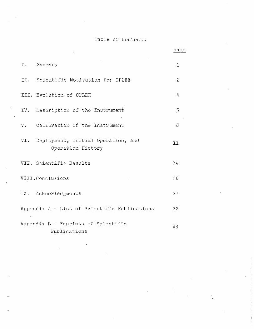
Table of Contents

I. Summary

II. Scientific Motivation for CPLEE

III. Evolution of CPLEE

IV. Description of the Instrument

V. Calibration of the Instrument

VI. Deployment, Initial Operation, and

Operation History

VII. Scientific Results

VIII.Conclusions

IX. Acknowledgments

Appendix A - List of Scientific Publications

Appendix B - Reprints of Scientific

Publications

1

2

4

5

8

11

20

21

22

23

-1-

SUMMARY

This is the final technical report on the contract

NAS9-5884 awarded by the National Aeronautics and Space

Administration to Rice University for the Charged Particle

Lunar Environment Experiment (CPLEE). CPLEE is ion-electron

spectrometer placed on the lunar surface for the purpose of

measuring charged particle fluxes impacting the moon from a

variety of regions and to study the interactions between

space plasmas and the lunar surface.

Principal accomplishments under this contract were:

1. Furnishing design specifications to Bendix

Research Laboratories for construction of the

CPLEE instruments.

2. Development of an advanced computer-controlled

facility for automated instrument calibration.

3. Active participation in the deployment and

past-deployment operational phases with regard to

data verification and operational mode selection.

4. Publication of numerous research papers, including

such Varied facets as a study of lunar photoelectrons,

a study of plasmas resulting from man-made lunar

impart events, a study of magnetotail and magneto­

sheath particle populations, and a study of solar­

flare interplanetary particles.

This report describes these past accomplishments in

detail along with plans for future research programs using

data from the instrument.

-2-

Scientific Motivation for CPLEE

The scientific justifications for placing a charged

particle spectrometer such as CPLEE on the lunar surface are

quite simply to measure the fluxes, energy spectra, and

charge types of charged particles bombarding the lunar

surface and to investigate the interaction of these particles

and other forms of radiation with the lunar surface.

In one view the moon is a satellite with an orbital

radius of 60 RE (earth radii) that c~rries the CPLEE instrument

through various regions of physical and scientific interest.

Figure 1 shows a typical lunar orbit in relation to the

geometry of the earth's magnetospheric system and interplanetary

space. The arrows show the look directions of the two

charged particle analyzers in CPLEE. It is seen that once

per lunar month the lunar orbit carries the instrument

through the di~tant magnetosheath, magnetotail, and regions

of direct access to the solar wind and finally (during

periods of new moon) the instrument is viewing into the

downstream cavity carved into the solar. wind by the moon.

Thus an opportunity is afforded to investigate a wide variety

of particle phenomena; charged particles in the geomagnetic

tail (the plasma sheet), magnetosheath fluxes, fluxes at the

boundary between the geomagnetic tail and the magnetosheath

(the magnetopause), the solar wind shock, and direct solar

wind particles. The relative magnitudes and temporal relationshps

between these particles in the distant lunar regions and

particles nearer the earth measured by other satellites can

be measured.

In another sense, the instrument is capable of measuring

the interactions of particle and photon radiation with the

lunar body itself. The size scale of the moon is comparable

to or larger than typical scale sizes of the particle fluxes,

and hence one would expect on occasion significant interactions.

Figure 1

A schematic plan of the lunar orbit in relation

to the earth's magnetospheric system and interplanetary

space. The arrows show the look direcitons of the instrument

det~ctors.

TO THE SUN

XSE

LOOK

DIREC TIONJ

~ ~ALSEP 14 . SUNSET

~. "

-3-

An example would be a possible shock wave near the teminator

regions due to solar-wind lunar limb interactions. A second

example would be the photoelectron layer generated by solar

photons striking the surface, and measurement of these can

only be made by a surface-based instrument.

Thus there are numerous scientific justifications and

expectations in placing a charged particle spectrometer on

the lunar surface. In subsequent sections of this report it

will be seen how many of these expectations have been fulfilled.

-4-

The Evolution of CPLEE

The concept of the CPLEE instrument grew from an active

program of auroral sounding rocket research at Rice University

during the years 1963-1968. One of the objects of the

auroral research program was to make detailed, high time

resolution measurements of the auroral charged particle

spectrum over as wide an energy range as possible. Along

with this requirement went the usual constraints of low

weight, power, and size made necessa~y by the constraints of

the research vehicle. Accordingly, an instrument code-named

SPECS (Switching Proton-Electron Channeltron6 Spectrometer)

was developed to meet these requirements. SPECS consisted

of an electrostatic particle deflection system and an array

of six Channeltron6 detectors to separate and detect particles

according to energy and charge sign. In its final evolutionary

stages, the instrument made a 15-point measurement of the

spectra of both ions and electrons with energies ranging

from 40 electron volts to over 20,000 electron volts. The

time required to complete a measurement cycle could be

varied, but for most applications was on the order of a few

seconds.

SPECS instruments were flown on each of a series of

three Javelin sounding rockets in February, 1967 and February,

1968. In addition, a SPECS instrument was successfully flown

on a Rice/ONR auroral research satellite code-named Aurora

I in June of 1967 and operated successfully for over one

year. Thus the basic detector design was well-proved in

space applications and environments well before the actual

CPLEE lunar deployment, and the cognizant scientists were

able to gain considerable experience in analyzing data from

the basic instruments years in advance of the CPLEE mission.

6Registered Trademark, Bendix Corporation

-5-

Description of the CPLEE Instrument

The CPLEE consists of a box supported by four legs.

The box contains two similar physical charged-particle

analyzers, two different programable high-voltage supplies,

twelve 20-bit accumulators, and appropriate conditioning and

shifting circuitry. The total weight on Earth is approximately

2.7 kg (6 lb.), and normal power dissipation is 3.0 W rising

to approximately 6 W when the lunar-night survival heater is

on.

Each physical analyzer contains five C-shaped channel

electron multipliers with a nominal aperture of 1 mm each

and one helical channel electron multiplier with a nominal

aperture of 8 mm. These are shown schematically in Figure 2.

The channel electron multiplier is a hollow glass tube,

the inside surface of which, when bombarded by charged

particles, ultraviolet light, etc., is an emitter of secondary

electrons. In the CPLEE, the aperture of each electron

multiplier is operated nominally at ground potential (actually

at 16 V), while a voltage of 2800 or 3200 V (selected by

ground command) is placed on the other (i.e., anode) end.

Thus, if an incident particle enters the aperture and secondary

electrons are produced, these are accelerated and hit the

walls to generate more secondary electrons, so that a multipli­

cation to an order of 107 is achieved by the time the pulse

arrives at the anode. After conditioning, pulses from each

electron multiplier are accumulated in a register for later

readout as described in the following paragraphs.

As shown in Figure 2, incident particles enter an

analyzer through a series of slits and then pass between two

deflection plates across which a voltage can be applied.

Thus, at a given deflection voltage, the five small-aperture

electron multipliers make a five-point measurement of the

Figure 2

A schematic drawing of the charged-particle analyzer

in the CPLEE instrument. Particles pass through a series of

collimators, and are then deflected by a set of electrostatic

deflection plates onto an array of six channel electron

multipliers.

-6-

energy spectrum of charged particles of a given polarity

(e.g., electrons), while, simultaneously, the large-aperture

electron multiplier makes a single wideband measurement of

particles with the opposite polarity (e.g., protons). The

advantages of simultaneously measuring particles of opposite

polarity and of simultaneous multiple-spectral samples are

considerable in studies of rapidly varying particle fluxes.

In the CPLEE, the deflection-plate voltage, in the

normal mode, is stepped in the sequence shown in Figure 3. As a consequence, the energy passbands shown in Figure 4 are sampled. Although data acquired by the six sensors are

not transmitted simultaneously, the sjx sensors are connected

to six accumulators for exactly the same time (viz, 1.2 sec)

and the contents transferred to shift registers for later

sequential transmission.

Two analyzers, A and B, point in the directions shown

in Figure 5. The same deflection voltage is applied to each

analyzer simultaneously, with counts from 1.2-sec accumulation

time of analyzer A being transmitted while counts from

analyzer B are accumulating. Thus, each voltage is normally

on for 2.4 sec with the result that the total cycle time is

19.3 sec (Fig. 3), when allowance is made for two sample

times when the deflection voltage is zero. On one of those

two occasions, counts are accumulated as usual to measure

background or contaminating radiation. On the other occasion,

a pulse generator of about 375 kHz is connected to the

accumulators to verify operation.

The command link with the ALSEP provides a variety of

options for CPLEE operation. Aside from the usual power

commands corrc1on to ali ALSEP exper1ments, three commands are

provided that allow the normal automat1c stepping sequence

to be mod1fied. The sequence can be stopped and then the

deflect1on plate supply can be manually stepped to any one

of the e1ght poss1ble levels. This 1s done to study a

Figure 3

The deflection voltage stepping and analyzer

switching sequence of CPLEE. In the automatic mode, a

complete cycle is completed in 19.3 seconds. In the manual

mode, the deflection voltage stepper is halted at one of the

eight possible levels, and the analyzers are read out

alternately with a cycle time of 2.4 seconds.

CPlEE TIMiNG SEQUENCE ALSEP I FRAME NO O

VOLTAGE

-

I 4

I I I I I I I 8 12 16 20 24 28 32

READOUT OF A DURING B MEAS , ETC.

CAL

EVEN FRAME MARKS -3500

~-~~~------19. 3 SEC (NORMAL)----~

Figure 4

A schematic representation of the energy pass­

bands of CPLEE. The energy passbands are shown for each

of the three deflection voltage levels of 35, 350, and

3500 volts.

CPLEE ENERGY PASSBANDS

6

3500 I I VOLTS I 2 3 4 5

0 0 0 o· I I 6

350 I I VOLTS I 2 3 4 5

DOD D I I 6

35 I I VOLTS I 2 3 4 5

DO 0 D I I t l I

.01 .I 10 100

PARTICLE ENERGY ( KeV)

Figure 5

The CPLEE system, showing the locations and look

directions of the two analyzers. ·

CHARGED-PARTIClE lUNAR Et~V~ROt~r~Ef~T

EXPER~MENT SUBSYSTEM

PHYSICAL ANALYZER

ELECTRONICS

-7-

particular phenomenon (e.g., low-energy electrons) with

higher time resolution (2.4 sec). A second set of commands

allows the electron-multiplier high-voltage supply to be set

at either 2800 or 3200 V. The higher voltage is used in the

event the electron-multiplier gains decrease during lunar

operations. A third pair ·of commands allows the normal

thermal-control mode to be bypassed in the event of failure

of the thermostat, thus offering manual control of the

heaters. A summary of the command structure and of the

engineering housekeeping measurements is shown in Figure 6. The CPLEE apertures are covered with a dust cover to

avoid contamination during deployment and, particularly,

during LM ascent. The dust cove~ was made doubly useful

because a Ni 63 radioactive source was placed on the underside

over each aperture.

on the Moon, and the

the same way with the

calibrated on Earth.

Thus, the sensors were proof calibrated

data compared with measurements made in

same system when the unit was last

The results of the Ni 63 beta source

tests at times of pre-calibration, post-calibration, and

post-deployment are shown in Figure 7.

Figure 6

The engineering housekeeping measurements, red­

line limits, and co~nand structure of CPLEE.

[ij

TM. ~ NORMAL ..: OPERATING RED-LINE

MEAS. I DESCRIPTION u RANGE LIMITS NO. X

"" LOW HIGH LOW HIGH , AC-1 25 Switchoblt Power Suppl~ Votto9e II 244 5 250

-PCM Counts

AC-2 89 Channaltron F.'S. HI Volta~e 2BOOv 3200v 2400v 3600v Monitor Analyzer 8

AC-3 40 Chonnaltron r s. ~2 Voltage 2800v 3200v 2400v 3600v Monitor Analyze-r A

AC-4 10 OC-to- DC Converter Voltage + 2.Bv • 3.2v .f.2.6v + 3.4v

AC-5 II Physical Ana tyzer Temp. -1e•c ~38°C -45°C +613°C

AC-6 0 Swl1chob/e Power Supply Temp. -1e•c +38°C -45•c +6S'C

Table 2-30 CPLEE Comond List

Command Number Octal Nomenclature

I Ill Operation a I heater ON 2 112 Operational heater OFF

3 113 Dust cover removal

4 114 A·Jtomotic voltage sequence ON

5 115 Step voltage level

6 117 Automatic voltaoe sequence OFF

7 120 Chonnellron ® voltooe increase ON

B 121 Chonne!tron ® voltage increase OFF

Figure 7

A summary of the Ni 63 beta source test performed

before and after instrument calibration, and after lunar

surface deployment prior to dust cover removal.

CPLEE BETA SOURCE TESTS

ANALYZER A

CHI CH 2 CH 3 CH 4 CH 5 CH 6

Pre- Cal. 8.7 22.2 38.8 80.7 165.7 1280.5

Oct.24, 1969

Post-Cal. 8.2 18.9 38.5 86.6 205.7 1323.0

Jan. 20,1970 Post- Deploy

10.68 20.5 39.6 82.4 195.9 1259.0 Feb. 6-1971

ANALYZER 8

CHI CH 2 CH 3 CH 4 CH 5 CH 6

Pre-Cal. 5.8 12.7 19.8 43.6 113.1 777.7 Oct. 24, 1969

Post-Cal. 4.5 9.1 14.6 34.8 96.6 577.9 Jan. 20, 1970

Post- Deploy 7.68 12.0 17.8 35.4 90.0 763.8 Feb. 6, 1971

-8-

Calibration of the CPLEE Instrument

Although the process of calibration of a scientific

detector is usually viewed as a prosaic task, some rather

challenging technological problems had to be solved in this

endeavor and therefore it is worthwhile to examine in some

detail the calibration procedure and the system that was

developed to accomplish this procedure.

The object of calibration of any charged particle

detector is to obtain a number which· relates the counting

rate from the instrument to the particle flux incident upon

the instrument. For particle fluxes usually encountered in

space measurement situations, a convenient unit for particle

flux is particles/square centimeter-second-steradian-electron

volt (part./cm2-sec.-ster.-eV). This unit then measures the

number of particles crossing a unit square centimeter

each second, from a cone of arrival directions subtending

one steradian in an energy interval one electron-volt in

width. In mathematical terms, if we let C.R. be the counting

rate of the detector and j(E) be the incident flux, then:

C.R. = J 0

j(E)A(E)Q(E)E(E)dE

where A(E), n(E), and E(E) are quantities determined by the

detector geometry and are defined in the following manner.

A(E) is the effective area of the detector (cm2 ), n(E) is

the effective solid angle of the detector, which is related

to the angular response, and E(E) is the efficiency of the

detector, expressed in counts/particle. Thus if one can

obtain a plot of the product A(E)n(E)E(E) as a function of

energy, then one can in principle unfold the integral relation

shown above to obtain j(E) if the counting rate is known.

Parenthetically, the plot of the product A(E)n(E)E(E) vs. E

is commonly known as the energy passband of the detector.

-9-

The task of calibration is then to determine A(E),

(E), and (E) either singly or in product form. Conceptually

this would appear simple since one has only to create a

particle beam of known intensity, impress it upon the detector,

and observe the counting rate. The problem arises however

when one considers that one is interested in the response to

beams distributed in arrival angle whereas beams available

in the laboratory are most easily generated unidirectionally,

that is all particles have the same direction. Therefore,

if a unidirectional beam is applied to the instrument from a

given arrival direction and , then one actually measure

the product A(E) (E) at a given energy and arrival direction.

To obtain (E) it is then necessaTy to repeat the measurement

for a number of arrival directions sufficient to include the

complete angular range of instrument sensitivity.

Now the magnitude of the calibration problem can be

appreciated. In CPLEE there are two analyzers that each make

an 18-point spectral measurement. Thus, for electrons only

(say), there are 36 separate energy passbands that must be

determined. It was desired to take 10 energy points per

passband, and so this involves 360 separate energy runs.

Each one of these runs in turn requires measurement at

numerous angles. In particular, the desired angular grid turned

out to be 10° x 20° in 0.5° steps each axis, requlrlng 861

separate angle steps. This works out to more than 3 x 105

separate measurements to calibrate one CPLEE for electrons

only. Considering that the program called for calibration

of four units (prototype, two flight units, and flight

spare) plus calibrations of each for sensititivty to solar

ultra-violet radiatiori, it quickly became obvious that

traditional means involving manual setting of angles, reading

data, and hand reduction could not possibly fulfill the

requirements. Accordingly, the decision was made to develop

a computer-controlled calibration facility that could function semi­

automatically with a minimum of operator attention required.

-10-

The basic requiren1ents for such a calibration system

were then: 1. A stable source of electrons capable of

producing beams with energies ranging from 40 eV to over

20,000 eV; 2. A mechanical fixture to position the instrument

at various angles relative to the beam; 3. Fixture drive

motors and angle position indicators capable of computer

control and readout; 4. A computer system capable of posi­

tioning angles, reading data, storing data, and monitoring

various engineering parameters in an automatic sequence; 5.

A vacuum chamber of sufficient size to contain the electron

gun, fixture, and instrument; 6. A number of competent

personnel to make it all function~

The various required components, included a SDS-92

computer, a Varian vacuum system, and numerous items such as

power supplies, etc. were purchased and assembled into the

calibration system. The mechanical accessories (i.e., the

fixture) were fabricated at Rice and also the logic circuitry

necessary to interface the computer with the CPLEE, the

fixture drive motors and angle indicators; and various other

measuring devices was designed and built at Rice. The

system became operational in August 1968. It was found that

approximately one month was required for a complete particle

and ultra-violet sensitivity calibration of one CPLEE.

An example of the calibration results for CPLEE is

shown in Figure 8, showing the analyzer A electron passbands

for all eighteen energy channels. These were determined from

the calibration of CPLEE SN-5, the flight unit for the

Apollo 14 ALSEP. Three passbands are shown for a given

channel, corresponding to each of three values of electrostatic

deflection voltage; 35, 350, and 3500 volts. It is seen

that the passbands for a given channel are nearly identical

when the factor of 10 changes in the energy scale are

considered. In practice, these passbands were numerically

integrated to obtain a number GFo x 6E, with GFo x 6E = IQF(E)dE and GF(E) = A(E)n(E)E(E). GFo was set to be numerically

equal to the peak value of GF(E), and therefore 6E is an

effective passband width. Operationally then, the fluxes

were determined from the relation j(Eo) = C.R./(GFo x 6m.

Figure 8

The electron energy passbands of Analyzer A,

CPLEE S/N 5 as derived from the calibration.

·• I X 10

0

0

0

20a!0•4

16

12

0

DETECTOR 1

40 400

••

100

" lOt

200 .. 20t

+30

)

300 .. 30t

ANALYZER •

400 •• 40k

60 600 ..

000 .. 50k

600 6t 60t

70 700 H

130 1300 Ilk

700

" 70t

Oo·------~~~,~~------,lo-o-----~~~----------,,o-o--------~----------,~o-o---------, ~00 1000 zooo :5000 511 1011 ZOII

Energy (eV)

-11-

Deployment, Initial Checkout, and

Operational History

The CPLEE was deployed with no dificulty at approxi-

mately 18:00 G.M.T. on February 5, 1971. Leveling to within

2.5° and east-west alinement to within + 2° were to be

accomplished with a bubble level and a Sun compass, respectively.

A photograph of CPLEE on the lunar surface is shown in Figure 9.

It has since been determined by· a careful study of the

lunar photographs and a comparison of predicted and actual

solar ultraviolet response profiles that the experiment is

1.7° off level, tipped to the east, and 1° away from a

perfect east-west alinement. This error is well within the

preflight specifications.

The CPLEE was first commanded on at 19:00 G.M.T.,

February 5, 1971 during the first period of extravehicular

activity for a brief functional test of 5-min duration. All

data and housekeeping channels were active, and the instrument

began operation in the proper initial modes (i.e., automatic

sequencer, on; electron-multiplier voltage increase, off;

and automatic thermal control, on).

A complete instrument checkout procedure was initiated

at 04:00 and continued until 06:10 G.M.T., February 6, 1971.

During this period, data from the dust-cover beta sources

were accumulated and compared with prelaunch calibrations.

These tests showed no significant changes in the instrument

calibration. Also during this period, all command functions

of the CPLEE were exercised except the forced heater mode

and dust-cover removal commands. The instrument responded

perfectly to all commands. After the checkout procedure,

the CPLEE was commanded to the standby mode to await LM

ascent.

Following LM ascent, the CPLEE was commanded on at

19:10 G.M.T. and the dust cover was succe~sfully removed at

Figure 9

A photograph of the CPLEE instrument on the lunar

surface. The dust cover is in place. The bubble level is

visible adjacent to the letter "E" and the sun compass, read

by the position of the handling tool shadow, is visible

at the opposite end of the instrument.

-12-

19:30 G.M.T., February 6. The CPLEE immediately began

returning data on charged-particle fluxes in the magnetosphere.

The instrument temperatures were carefully and continuously

monitored for 45 days after deployment. It was found that

the temperature range was nominal, with the internal electronics

temperature ranging from 58° C at lunar noon to -24° C

during lunar night. The total lunar eclipse of February 10

offered an excellent opportunity to determine various thermal

parameters and to test the capability of the CPLEE to survive

extreme thermal shocks. A plot of the physical-analyzer

temperature during the eclipse is shown in Figure 10. The

maximum thermal shock occurred after umbra exit, with a

temperature change rate of 25° C/hr. Also from this figure,

it is possible to derive a thermal time constant of approxi­

mately 1.9 hr. The CPLEE suffered no ill effects from this

period of rapid temperature changes. The command capability

of the CPLEE was used extensively during the 45-day real-

time support period to optimize scientific return from the

instrument. Alternate 1-hr periods of manual operation at

the -35 V step and automatic operation were used to concentrate

on rapid temporal variations in low-energy electrons.

Similarly, alternate periods of 350 V manual and automatic

operation were used to focus on rapid changes in magnetopause

ions and the solar wind. In fact, the manual operation

capability and the attendant 2.4-sec sampling interval made

possible the detection of phenomena that would have been

impossible to detect otherwise because of sampling problems

and aliasing. Most of the decisions concerning operational

modes were based on viewing the real-time data stream.

On April 8, 1971 at 21:55 the housekeeping monitor for

the Analyzer B Channeltron high voltage supply showed a

serious undervoltage condition. Subsequent analysis of the

data tapes showed that this was a sudden failure, the voltage

having decreased from its nominal value of 2800 volts to

approximatley 800 volts within one housek~eping data cycle

Figure 10

A plot of the temperature profile of CPLEE during

the lunar eclipse of February 10, 1971.

-u +60 0 -w ~ +50

~ n:: w Q_

~ w ~

n:: w N

+40

+30

~ +20 <! z <! _j +10 <! u (f)

>- 0 I Q_

-10

<( 0:::: CD ~ :::)

z w a.. 0:::: w 1--. z w t

CPLEE TEMPERATURE PROFILE LUNAR ECLIPSE

FEBRUARY 10, 1971

~ CD :::E :::::> z w Cl..

1-

0500 0600 0700 0800 0900 1000 1100 1200

UNIVERSAL TIME

1300

-13-

period. The instrument was placed into standby for the

remainder of the lunar day period and operation with Analyzer

A only was resumed on April 16, 1971. A meeting was held

with representatives of JSC, Bendix, and Rice University

where it was determined that the most probable cause of the

failure was either a failure of a component in the high

voltage rectifier assembly or an arc track developing in the

high voltage supply encapsulating material.

The instrument continued to operate returning Analyzer

A data only until June 6, 1971. At that time a low voltage

condition (1800 volts) appeared in the Analyzer A Channeltron

high voltage supply, rendering the Channeltrons inoperative.

The decision was made to place the instrument into standby

and continue testing during the subsequent lunar night

period.

It was discovered that the instrument would operate for

short periods during the lunar night (l/2 hour) before the

high voltage decreased to the point where Analyzer A was

inoperative. This pointed to a temperature-dependent effect

wherein normal voltage could be develop~d when the instrument

was cold but local heating effects would soon cause degradation.

It was also learned that, as time went on, longer and longer

periods of lunar night operation were possible and beginning July of

1972 operation during the entire lunar night was possible.

Furthermore, operation was possible for portions of the

lunar day. In December, 1972 at the commencement of the

real-time support period for the Apollo 16 mission the

instrument was turned on at lunar morning and continued to

operate continuously throughout the lunar day. However, in

April, 1973 a second partial failure of the high voltage

supply occurred which again restricted operation to lunar

night periods only. This condition has continued to the

present day.

-14-

Scientific Results of the CPLEE Program

In this section we discuss the scientific results of

the CPLEE program. As this report includes reprints of most

of the CPLEE scientific publications, only summaries will be

presented here.

A prominent feature of data obtained while in the

geomagnetic tail was a stable, low-energy electron popula-

tion with energies ranging from 40 to 200 electron volts.

Although possibly due to a low energy magnetospheric population,

a plot of their flux during the lunar eclipse of February

10, 1971 revealed their origin to be of photoelectric

origin (Figure 11). Their correlation with sunlight upon

the lunar surface shows that these fluxes were due to photoelectrons

gen.erated by solar photons strildng the lunar surface. A

plot of their energy spectrum is shown in Figure 12, showing

that a) the photoelectrons were essentially isotropic over

the upper hemisphere and b) the highest energy was about 200

electron volts. Recalling that the instrument detects those

photoelectrons which are returning to the surface, this

means that the sunlit lunar surface potential when the mo0n

is in the magnetotail away from the plasma sheet i.s on the

order of 200 volts with respect to the surrounding medium.

The impact of the Apollo 14 Lunar Module offered an

opportunity to study any charged particle fluxes resulting

from the impact. The impact point was 66 km west of the

CPLEE location. Figure 13 shows a time history of particle

fluxes resulting from the impact. This plot shows fluxes of

70 ev ions and 65 ev negative particles. It is seen that

approximately one minute after impact, two plasma "clouds"

passed the instrument. These ions could not have been generated

at the moment of impact, for had that been the case the

particles would have appeared less than one second after

impact. Rather, it was postulated that the impact produced

expanding neutral gas clouds, and constituents of this cloud

Figure 11

The counting rate of Channel 6, +35 volts sensitive

to electrons with 50 eV< E< 150 eY during the lunar eclipse

of February 10, 1971. The disappearance of the fluxes

during the eclipse shows that the electrons are of photo­

electric origin.

104

~r CPLEE ANALYZER A 50-150 ev ELECTRONS

<! 0:: LUNAR ECLIPSE CD <( ::2! FEB. 10, 1971 0:: ::::J (I)

103 z ~ w

0.. :J z

(.) 0:: <! w .Q) w 0:::: a..

r- m {/) z ~ t-

C\J w :J -- 0::: X - w .......... w t-r- -(/) z X

w w t-z :::)

0 u

I~ ~ IJ1~ ' ~~

10 'f r r i!.

i l '•

0500 0600 0700 0800 0900 1000

UNIVERSAL TIME

Figure 12

The lunar surface photoelectron spectrum measured

by CPLEE. The geometries relative to the surface and to the

incoming photon flux are shown in the inset.

> 105 Q)

I 0::: w ._. (f)

I 0 w (f)

I 104

C\J ~ u .......... (f)

z 0 0::: ._. u w 103 _J

w

CPLEE PHOTOELECTRON SPECTRUM

ANALYZERS A AND B

\ \ \

~ \/8

\ \ \ \ \ \ \ ~

B

E (.)

<.D

"' SURFACE

102 ~--~----~----~----~--~----~----~ 280 40 80 120 160 200 240 0

ELECTRON ENERGY (ev)

Figure 13

Ion and electron fluxes resulting from the impact

of the Apollo 14 Lunar Module upon the lunar surface.

100,000.--.-----.-------r----.-------,-------,

G 1o,ooo w (f)

N

' (f) f­z ;:)

0 ~

~ 1000 _J (._)

f-a:: ~ w > f­<l: (.9

w 100 z

CPLEE ANALYZER'~'

APOLLO 14 LM IMPACT

/70 ev ions

~65 ev negative particles

IOL-_J_ ____ ~----L-~--+--~-~----~~ 038/00/44/53 038/00/46/29 038/00/48/07

1000

(._) w (f)

C\J -= ' (f) f-

100 z ;:)

0 (._)

10

-(f) z 0

38/00/45/41 038/00/4 7/18 038/00/48/55

UNIVERSAL TIME (DAYS/HOURS/MIN./SEC)

-15-

were then ionized and energized by interaction with the

solar wind. The implications of the results are that if

neutral gas is released upon the lunar surface by any means

then it could subsequently be carried away relatively rapidly

by strong interactions between the gas anq the solar wind.

A systematic study of particle fluxes in the geomagnetic

tail, the plasma sheet, was undertaken in order to determine

the average characteristics of these particles and their

response to geomagnetic storm activity. One question to be

considered is that of shadowing, that is "does the moon

effectively sweep out magnetic flux tubes of their particles

and thus prevent CPLEE from observing these particles?"

This question was answered by comparing CPLEE particle

observations with magnetic field data from the Explorer

35/Ames Research Center lunar-orbiting magnetometer. The

magnetometer indirectly indicates the presence of the plasma

sheet by a decrease in the magnetic field strength owing to

the diamagnetism of the plasma sheet particles. It was

discovered that in 90% of the cases when magnetic field

depressions were observed, particle fluxes were observed by

the CPLEE instrument. Thus for the majority of the time

plasma sheet fluxes are not shadowed from the lunar surface.

The average plasma sheet electron and ion spectra are

shown in Figure 14. The lowest energy portion of the spectrum

is due to the lunar photoelectrons. The plasma sheet spectra

represent electron and ion populations with ne = 0.1, Te = 200 eV, n. = 0.1, T. = 2.5 keV. These particle temperatures

l l

were found to be equivalent to temperatures measured in the

plasma sheet at 20 RE by the Vela satellites, but the number

density was 0n the average a factor of 5 less than that

measured at 20 Re.

A statistical study of plasma sheet encounters was done

in order to determine the vertical extent, or thickness of

the plasma sheet at the lunar distance. The thickness was

determined to be 5 + 2 RE' somewhat thinner than the value

Figure 14

The average plasma sheet electron and ion spectra

observed at the lunar distance. The lowest energy portion

of the spectrum was due to photoelectrons, and had to be

subtracted from the data in order to obtain the fitted spectra

shown

-> <1>

"-

~ 104 (/)

0 <1> (/)

C\1

E 0

' 103

(!)

0 ..... ~

0 a.. -

February 9, 1971 1946 G.M.T.

CPLEE Analy2er A • electrons

VACUUM/ PHOTOELECT CURVE

MAXWELLIAN nP = 0.1 kT = 2.5 keV

A ions

o average photoelectron levels

MAXWELLIAt-J ne =0.1 cm- 3

~ kT-= 200 eV

IO o ILO_L-..JL--L' .L.• L.l! !..J..J!I'o..J_I_o_L' __.__, _.l-L..Ll-l.J..J.I K_--L.--1..-JL-L..l..J...IL.LOI-K-.--lii--1

ENERGY {eV) ,f

-16-

of 6-12 RE measured in the range 20-30 RE from the earth by

other satellites.

The response of the plasma sheet to geomagnetic substorms

has also been investigated. It was found that at the onset

of a substorm a sudden, dramatic enhancement in the plasma

sheet flux appeared at the lunar orbit followed by a disappearance

of plasma until substorm recovery. The thinning, or disappearance

of the plasma sheet at substorm onset is a phenomenon observed

at distances closer to the earth, but the precursor spike

seems to be unique to the lunar distance and is quite possibly

a result of a pileup of plasma along the leading edge of the

thinning front.

Strong flows were observed in the netural sheet on two

occasions during substorms. At the time of substorm onset

the magnetic field normal to the neutral sheet was observed

to change direction and simultaneously a strong anti-solar

ion flow was observed. This is strong evidence that at the

time of substorms a neutral line, or a line of magnetic

field connection across the neutral sheet, is formed between

the earth and the moon. Plasma is accelerated away from the

neutral line, travelling both toward the earth and backwards

toward the moon.

On April 9, 1971 a large world-wide magnetic storm

occurred. Data from CPLEE, the Solar Wind Spectrometer

Experiment (SWSE), the Explorer 35/ARC Magnetometer, and

solar wind and magnetic field detectors on-board the Explorer

33 satellite were used for a detailed study of the response

of the distant geomagnetic tail to this storm. Figure 15

shows the geometry of the magnetosphere, the location of the

solar wind d~scontinuity prior to the storm, and the locations

of the detectors.

The storm was first signaled by ground-based magnetometer

disturbances at 0428 G.M.T. At 0543 magnetosheath particle

fluxes appeared at the moon and remained until after 1000.

Referring to the pre-storm geometry of Figure 15, it is seen

Figure 15

The geometry of the earth's magnetosphere relative

to the solar wind discontinuity and the locations of the

moon and the Explorer 33 satellite immediately prior to

the geomagnetic storm of April 9, 1971.

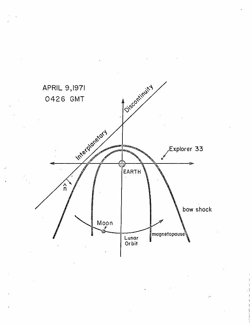
APRIL 9,1971

0426 GMT

Lunar Orbit

/Explorer 33

•

-17-

that the entire geomagnetic tail was compressed until the

magnetopause boundary crossed the position of the moon. The

radius of the geomagnetic tail decreased from 26 to 16 RE.

This was accompanied by an increase in the tail magnetic

field strength from 10 gammas to 32 gammaq. Multiple crossings

of the magnetopause boundary after 1000 G.M.T. coincided

with changes in the angular direction of the solar wind

flow, showing the influence of solar wind flow direction

upon the orientation of the geomagnetic tail. Finally, when

the moon was in the magnetosheath between 0545 and 1000

G.M.T. an electron population characteristic of the plasma

sheet was found to be superimposed upon the normal low-

energy magnetosheath electron population. This shows an

enhanced loss of plasma sheet particles into the magnetosheath

during periods of high magnetic activity.

The large solar flare event of August, 1972 was an

event of unusual magnitude and fortunately at the time the

moon was outside of the geomagnetic tail regions in interplanetary

space. Therefore there existed the opportunity of studying

particle fluxes resulting from the flares unmodified by

interaction with the earth's magnetic field. Plots of the

counting rates of analyzer A, channel 1 at the deflection

voltages +0 (background), -35 volts and -350 volts for the

period is shown in Figure 16. The count rate scales are

displaced by a factor of 10 vertically for the sake of

clarity. It is seen that after day 217 at 1200 hours the

counting rates were independent of deflection voltage,

indicating that these counts were due to high energy solar

flare particles that were capable of penetrating the instrument

case. This ~nterpret~tion was confirmed by cosmic ray

detectors on other satellites. However, between 0200 and

about 1200 on day 217 there are counting rates in the -35

and -350 channels that are not matched by corresponding

rates in the background channel, indicating a population. of

electrons present. A temporal history of the energy spectra

Figure 16

Counting rates in CPLEE Analyzer A channel 1 at

three deflection voltages during the solar flare events of

August 1972. The plots have been displaced by a factor of

10 vertically for clarity. The identical counting rates at all

deflection voltages after 1200 GMT on day 217 shows that

these counts were due to high energy protons penetrating the

instrument case.

u w (./)

N

(./)

.... z :::J 0 u

to'

CHANNEL NO. I

214 215 216

-350 v.

-35 v .

217 218 219 220 221 222

DAYS (GMT)

-18-

of these electrons is shown in Figure 11. Here the horizontal

scale is energy and the vertical scale is flux. The spectra

represent averages over sixteen minutes. The most likely

explanation for these electrons is that they were generated

at the earth's bow shock by the interaction between the

shock and the strongly disturbed solar wind, and that these

electrons subsequently propagated upstream to the location

of the moon.

In summary, the principal scientific results of the

CPLEE program were:

1) Observation of a layer of lunar photoelectrons above

the sunlit lunar surface. From these data the lunar

surface photo yield and potential in the high­

latitude geomagnetic tail were calculated.

2) Observation of a strong interaction between the

solar wind and neutral gas clouds produced by

the Apollo 14 Lunar Module Impact. This interaction

produced charged particles with energies ranging

up to 100 eV.

3) Determination of the average spectral and spatial

characteristics of the plasma sheet at the

lunar distance.

4) Discovery of neutral line formation between the

earth and the moon and of strong anti-sunward plasma

flow during magnetic substorms.

5) De~erminati6n of the response of the distant

geomagnetic tail and magnetosheath to the geomagnetic

storm of April 9, 1971.

Figure 17

Electron spectra observed in August 1972 resulting

from the solar flare events.

-19-

6) Observation of a hot electron gas in interplanetary

space resulting from the August, 1972 solar flare

event.

7) Discovery of an energetic electron population in the

dawn-side magnetosheath that is strongly influenced

by geomagnetic activity. These particles were

shown to be capable of being a source of plasma

sheet particles.

Only summaries of the scientific results have been

given here. For further details the reader should consult

the publication reprints in Appendix B.

-20-

Conclusion

The CPLEE program has been seen to have been an outstanding

technical and scientific achievement. Of no small consequence

has been the educational benefits of the program. One

student (Frederick J. Rich) received his Ph.D. degree in

1973 as a result of CPLEE data analysis and another student

(Patricia R. Moore) will receive a M.S. degree in the spring

of 1974 and will continue research into CPLEE data leading

to the Ph.D. degree in 1975. Furthermore, the technical

capability of our laboratory was significantly upgraded by

the demands of the program.

Analysis of CPLEE data is by no means complete. Small

but significant fluxes of particles bombard the lunar surface

throughout the lunar night when the instrument is viewing

into the solar wind cavity downstream of the moon. It is,

of course, the natural proclivity of an investigator to look

at data with the largest counting rates first, and so these

lunar night data have been largely neglected. However,

studies of these data in conjunction with ion data from the

Suprathermal Ion Detector (SIDE) and from the Explorer

35/ARC magnetometer hold promise for a deeper understanding

of interaction between the moon and the solar wind and of

particle energization processes at the earth's bow shock.

These investigations have been proposed and accepted for the

Post-Apollo Program of Data Analysis and Synthesis.

-21-

Acknowledgments

The people who have contributed to the success of the

CPLEE program are numerous. The contribution of the original

principal investigator, Dr. B. J. O'Brien, who conceived the

project and brought it through the original stages must be

acknowledged. At Rice University, John T. Musselwhite and

Wayne A. Smith in their ~equential roles as project managers

contributed greatly. Messers. Keith Phelps, John 0. McGarity

and David S. Nystrom designed and built the calibration

systems, developed data reduction computer programs, and

provided technical assistance. Mr. Walter R. Lytz, Research

Administrator provided valuable assistance in contract

liaison.

Personnel at Bendix Research Laboratories and Bendix

Aerospace Corporation that must be mentioned are Messers.

John Iaunnou, Alan D. Robinson, Robert Miley, Mark Brooks,

Lowell Ferguson, and Jerome Pfeiffer.

At the Johnson Space Center (formerly Manned Spacecraft

Center) significant contributions were made by Messers.

Ausley B. Carraway, Mac McDonald, W. F. Eichelman, John

Lobb, Keith Kundel, J. B. Thomas, and J. L. Stringer.

At N.A.S.A. Headquart~rs, Messers. Richard Allenby,

Donald Beattie, Edward Davin, and William O'Bryant made

important contributions.

There are undoubtly persons who should have been included

in this list. Their absence indicates not a lack of contribution

but rather this writer's lapses in memory.

··~

-22-

Appendix A

Publications and Constributed Publications

Publications

Burke, \AI. J. and D. L. Reasoner , "Absence of the Plasma

Sheet at Lunar Distance During Quiet Times", Plan.

Space Sci.,~, 429, 1972.

Reasoner, D. L. and B. J. O'Brien, "Measurement on the

Lunar Surface of Impact- Produced Plasma Clouds",

J. Geophys. Res., TI, 6671, 1972.

Reasoner, D. L. and W. J. Burke, "Characteristics of the

Lunar Photoelectron Layer in the Geomagnetic Tail",

J. Geopbys. Res., 77, 6671, 1972.

Reasoner, D. L. and \v. J. Burl<:e, "Direct Observation of the

Lunar Photoelectron Layer'', Proceedings of the Third

Lunar Scienc_e Confer~nce, Vol. 3 ( ed D. R. Criswell)

MIT Press, 1972.

Rich, F. J., W. J. Burke, D. L. Reasoner, D. S. Colburn,

and B. E. Goldstein, "Effects on the Geomagnetic Tail

at 60 R of the Geomagnetic Storm of April 9, 1971", e J. Geophys. Res.,~' 5477, 1973.

Rich, F. J., D. L. Reasoner, and \AI. J. Burke, "Plasma

Sheet at Lunar Distance: Characteristics and Inter­

actions with the Lunar Surface", J. Geophys. Res.,~'

8097, 1973.

Moore, P. R., D. L. Reasoner, and W. J .. Burke, "Particles

on the Night Side of the Moon Associated with the

August, 1972 Solar F'lares", World Data Cen~er A, Report

UAG-28, (ed. Helen Coffey), p. 356, USDC, 1973.

Rich, F'. J., W. J. Burke, D. L. Reasoner, and E. W. Hones, Jr.,

"Plasma Sheet at Lunar Distance during filagnetospheric

Substorms", accepted for publication in J. Geophys.

;B_es~, 197 4.

Contributed Publications

Burke, W. J. and D. L. Reasoner, "Absence of the Plasma Sheet

at Lunar Distance During Quiet Times II' EOS' rrrans.

Am. Geophys. Union, 2£, 906, 1971.

Reasoner, D. L. and W. J. Burke, "Direct Observation of the

Lunar Photoelectron Layer", EOS, Trans. Am. Geophys.,

Union, 52, 910, 1971.

Rich, F. J., D. L. Reasoner, and E. W. Hones, "Time History

of Plasma Observations in the Geomagnetic Tail During a

Substorm", EOS, Trans. Am. Geophys. Union, .2J., 493, 1972.

Reasoner, D. L. and W. J. Burke, "Direct Observation of the

Lunar Photoelectron Layer", Proceedings of the Third LUnar

Science Conference, Supplement 3, Geochimica et

Cosmochimica Acta, 1972.

Moore, P.R., D. L. Reasoner, and W. J. Burl{e, "Particles

on the Night Side of the Moon Assobiated with the August, 1972

Solar Flares", EOS, Trans. Am. Geopllys. Unio~, .2J., 1056,

1972.

Reasoner, D. L., W. J. Burke, and F. J. Rich, "Observed Effects

on the Geomagnetic Tail at Lunar Distance of the April 9, 1971 Geomagnetic Storm", EOS, Trans. Am. Geophys. Union,

53, 1100, 1972.

Burke, W. J., D. L. Reasoner, and F. J. Rich, "Some Consequences

of the Large Scale Compression of the Magnetotail during

the April 9, 1971 Geomagnetic Storm 11, EOS, Trans. Am.

Geophys. Union, 53, 1100, 1972.

Rich, 11'. J. , D. L. Reasoner, and W. J. Burke, "Consideration of

Lunar' Shadowing . of Magnetospheric Plasma II' §Q;?_, rrrans.

Am. GeS2J2hys. Union, 53, 1101, 1972.

Moore, P. R., D. L. Reasoner, and W. J. Burke, "Magnetosheath

Electrons at 60 Re"' EOS, rrrans. Am. Geophys. Unj_on, ~'

1181, 1973.

Reasoner, D. L. and W. J. Burke, "The Potential Distributj_on

in the Interaction Regj_on between the Plasma Sheet and

the Lunar Photoelectron Layer, EO~, Trans. Am. Geophys.

Union, 54, 1195, 1973.

-23-

Appendix B

Reprints of Publications

VOL. 77, NO. 7 JOURNAL OF GEOPHYSICAL RESEARCH MARCH I, 19i2

Brief Reports

Measurement on the Lunar Surface of Impact-Produced Plasma Clouds

DAVID L. REASONER

Department of Space Science, Rice University, Houston, Texas 77001

BRIAN J. O'BRIEN

Department of Environmental Protection, Perth, Australia

Simultaneous enhancements of low-energy ions and negative-particle fluxes due to the im­pact of the Apollo 14 lunar module were observed by the lunar-based charged-particle lunar­environment experiment (CPLEE). The impact occurred 66 km away from CPLEE, and the time delay between impact and flux onset was approximately 1 min. It is argued that the ob­served charged particles could not have energized at the instant of impact but rather that the impact produced expanding gas clouds and that constituents of these clouds were ionized and accelerated by some continuously active acceleration mechanism. It is further shown that the acceleration mechanism could not have been a static electric field but rather is possibly a con­sequence of interaction between the solar wind and the gas cloud.

The ascent stage of the Apollo 14 lunar module Antares impacted on the lunar surface on February 7, 1971, at OOh 45m 24s GMT. Shortly after the impact, a lunar-based charged­particle detector based 66 km away detected fluxes of low-energy positive ions and negative particles with intensities a factor of 10 greater than the ambient fluxes. The ion and electron enhancements exhibited near-perfect temporal simultaneity, and we report here preliminary studies of these impact-produced plasma clouds.

The measurements were made with the charged-particle lunar-environment experiment (CPLEE) deployed as part of the Apollo 14 Alsep instrument array at Fra Mauro. The CPLEE instrument is conceptually similar to the switching proton-electron channeltron spec­trometer (Specs) described in detail by O'Brien et al. [1967]. Two identical particle analyzers are housed in the unit. One analyzer, labeled A, is pointed toward the local vertical, and the other analyzer, labeled B, is pointed 60° from vertical toward lunar west.

We refer the reader to O'Brien et al. [1967] for a detailed description of the particle anal­yzers and report here a few salient features of

Copyright @ 1972 by the American Geophysical Union.

the instrument relevant to this report. Charged particles are deflected by a set of electrostatic deflection plates according to energy and charge sign into the apertures of an array of six chan­nel electron multipliers, and, at a given deflec­tion-plate voltage, an analyzer makes meas­urements of fluxes of particles of one charge sign (e.g., electrons) in five energy ranges and particles of the opposite charge sign (e.g., ions) in a single energy range. Normally the instru­ment steps through a series of six deflection voltages plus two background steps every 19.2 sec. However, the automatic sequence can be halted by ground command and the deflection voltage stepped to any one of the eight levels, with a consequent reduction of the sampling interval to 2.4 sec. Before the impact, the de­cision was made to operate the instrument in the manual mode at a deflection voltage where the instrument was sensitive to negative par­ticles in five energy ranges centered at 40, 50, 65, 95, and 200 ev, respectively, and sensitive to positive ions in a single energy range with peak response at 70 ev and half-intensity points at 50 and 150 ev. As will be seen, this decision proved extremely fortuitous.

The Antares impact occurred at lunar co­ordinates 3.42°S latitude and 19.67°W longi-

1292

BRIEF REPORT 1293

tude, a point 66 km west of CPLEE, at OOh 45m 24s GMT on February 7, 1971. The geom­etry of the impact event is shown in Figure 1. The terminal mass and velocity were 2303 kg and 1.68 kmjsec, respectively, resulting in an impact energy of 3.25 X 10" joules (G. V. Latham, private communication, 1971). The lunar module contained approximately 180 kg of volatile propellants, primarily dimethyl hydrazine fuel (CH.NHNHCH.) and nitrogen tetroxide oxidizer (N20,). There was an addi­tional source of energy if one considers the possibility of these hypergolic propellants com­bining. The heat of oxidation of dimethyl hy­drazine is 3.3 X 107 joules/kg [Goodger, 1970], and hence, if all of the propellants were able to combine, the energy released would be .-.3 X 10" joules maximum or comparable to the im­pact energy.

In Figure 2 are shown the counting rates of channel 6 of analyzer A, measuring positive ions with energies of 50 to 150 ev per unit charge, and of channel 3 of the same analyzer, measuring negative particles with energies of 61 to 68 ev, for the period OOh 44m 53s to OOh 48m 55s GMT on February 7, 1971.

As can be seen from Figure 2, the counting rates before and during Antares impact were reasonably constant. The preimpact counting

£:' 0 w j f-0 in n. <(

116 Km

rates in the low-energy negative-particle chan­nels were due to an ambient population of photoelectrons that was present whenever the lunar surface in the vicinity of CPLEE was illuminated. We note as proof of this assertion that these ambient fluxes disappeared entirely ·during the total lunar eclipse that occurred a few days later on February 10, 1971. The back­ground rate of the ion channel (channel 6) was due to various sources of contamination, including a small ( .-.6%) contribution from electron scattering within the analyzer. (This effect was well documented in preflight calibra­tions.) The ion-channel background level was essentially constant throughout the lunar orbit and hence was not due to a low-energy tail of the solar-wind ion flux.

f­Of­<(Z n.­:20 -"-

Beginning at T + 48 sec, a series of pro­nounced enhancements above background levels in counting rates of both the ion and the nega­tive-particle channels was observed, with the data dominated by two major enhancements centered at T + 58 sec and T + 74 sec, respec­tively. Because the enhancements were observed simultaneously in particles of both charge types, we refer to these events as plasma clouds.

The same data for analyzer B oriented 60° from vertical toward lunar west (i.e., toward the impact point) are shown in Figure 3. The

66Km

Fig. 1. A sketch of the geometry of the impact event, showing the location of the impact point relative to the location of CPLEE and the Apollo 12 Side instrument [Freeman et al., 1971]. Also shown are the incident solar-wind and assumed interplanetary magnetic-field

· ·directions.

1294 REASONER AND O'BRIEN

100,000

010,000 w (f)

"' ..... (f)

f-z ::J 0 2 (f) 1000 w _J

~ f-0: a: w ::::: f-<( <.9 w 100 z

--,-- ---1-

(expanded view~~ in figure 3) ! ) ... I

------ ~, ---~---.--------,

CPLEE ANALYZER ''A" APOLLO 14 LM IMPACT

"65 ev negative particles

1000

(.) w (f)

"' ' (f)

100 f-z ::J 0 2 (f)

z 0

10

JOL__L_ ____ 4-----L----4----L-----~~ 038/00/44/53 038/00/46/29 038/00/48/07

38/00/45/41 038/00/47/18 038/00/48/55

UNIVERSAL TIME (DAYS/HOURS/MIN./SE.C)

Fig. 2. The counting rates of channel 3 and channel 6 of analyzer A a.t -35 volts, meas­uring 65-ev negative particles and ions with 50 < E < 150 ev with peak response at 70 ev, respectively, showing the particle fluxes resulting from the lunar module impact.

background level of the ion channel in analyzer B is considerably higher than that for analyzer A for reasons that remain unknown to us. The effect however was well documented in a series of postdeployment tests with N :• beta sources that were attached to the underside of a re­movable dust cover protecting the analyzer apertures during deployment and lunar-module ascent. As for the analyzer A data, however, we measured the flux enhancement as the dif­ference between the instantaneous counting rate and the background level. From compari­son of Figures 2 and 3, one can note that the flux enhancements were essentially simultaneous in two directions, but the ion flux measured by analyzer A was 5 times higher than the ion flux measured by analyzer B. The geometric factors of the corresponding sensors in analyzers A and B are essentially identical, and hence the rela­tive flux magnitudes can be directly compared

by comparing the relative counting-rate en­hancements above the background levels of the channels. On the other hand, the negative-par­ticle flux measured by analyzer A was only one-third as great as the negative-particle flux measured by analyzer B. Examinations of Fig­ures 2 and 3 also show sporadic enhancements in particle fluxes occurring after the two initial plasma clouds. We consider that these enhance­ments were also the result of the impact but were due to various 'aftereffects,' perhaps sec­ondary impacts of ejecta material. (See dis­cussion below.) In this paper, therefore, we concentrate on the first two well-defined en­hancements.

The detailed characteristics of the two domi­nant plasma clouds are shown in Figure 4, a plot on an expanded time scale of the negative­particle fluxes in five energy ranges and ion flux in a single energy range measured by ana-

~'

BRIEF REPORT 1295

lyzer A. The plot shows clearly that the nega­tive-particle enhancement was confined to en­ergies less than 100 ev, since the 200-ev flux remained essentially constant throughout the event. The plot also shows that the enhance­ments of all the particles measured were simul­taneous to within the temporal resolution of the instrument (2.4 sec).

The negative-particle spectrum is seen (Fig­ure 4) to vary throughout the event in both the magnitude of the fluxes and the shape of the spectrum. A comparison of the preimpact negative-particle spectrum and the spectrum during the enhancements is shown in Figure 5. The first spectrum was measured at OOh 42m 38s, or during the period of stable, ambient fluxes some 3 min prior to impact. The second spectrum was measured at OOh 46m 21s, or during the first enhancement. The differing spectral shapes are clearly seen in this figure.

It might well be questioned whether the flux enhancements at T + 58 and T + 74 sec were actually initiated by the Antares impact. Indeed, in the time period of approximately 2

days following the impact event, when CPLEE was in the magnetosheath, several rapid en­hancements in the low-energy electron fluxes by up to a factor of 50 were observed. How­ever, these other enhancements were not cor­related with positive-ion flux increases, and, in fact, the event referred to here is the only such example of such perfectly correlated low-energy ion and negative-particle enhancements seen in this time period. In addition, careful monitoring prior to the impact revealed that the fluxes were relatively stable, constant to within a factor of 2 over time periods of a few minutes. These facts lend credence to the belief that this situation is a valid cause and effect one.

Further confidence in our interpretation that the flux enhancements were artifically impact­produced rather than of natural origin is gained by noting that although no such plasma clouds were previously detected resulting from impact events, Freeman et al. [1971] reported detec­tion of positive-ion clouds with the Apollo 12 supra thermal ion detection experiment (Side), which they concluded resulted from the Apollo

f-u <( Q

"' CPLEE ANALYZER "B" APOLLO 14 LM IMPACT

10,000 ::;: 1000

u w (f)

<:'>! .. .._. (f)

f-z :::> 0 8 (f)

w _j

u f-a: it w > i= <( t9 w z

_j

1000

100

~

65ev negative I particles

10~--L--A--~~~----~------~------~------~~

038/00/44/53 038/00/46/29 038/00/48/07

100

10

038/00/45/41 038/C0/47/18 038/00/48/55

UNIVERSAL Tl ME (DAYS/ HOURS/MIN./SEC)

Fig. 3. Same as Figure 2, except showing data from analyzer B.

0 w (f)

N

' (f)

f-z :::> 0 2 (f)

z '2

1296

>

"' I ~

"' -;;; u

"' U>

"' E ~ (f)

w _)

u i= 0: <! (L

REASONER AND O'BRIEN

L M IMPACT EVENT

103 ~-------------------------------------038/00/46/tt

UNIVERSAL TIME (DAYS/HOURS/MIN./SEC)

038/00/46/47

Fig. 4. An expanded view of the data of Figure 2, showing details of the two prominent peaks. Fluxes computed from five negative-particle energy ranges and one ion energy range are shown.

to7

" PRE-IMPACT NEGATIVE PLASMA CLOUD > ~ PARTICLE SPECTRUM ' NEGATIVE PARTICLE a>

SPECTRUM 0::

\ w I f-

to• ~ (f) I

u w (f)

~ \ "'I :::;:

to5t u '-(f)

~

~I w _J u

~ f-0:

a':

m'! I ~~_I

to' ~-·--'----L ----'--------' 0 80 t60 240 0 80 t60 240

ENERGY (ev) ENERGY(eV)

Fig. 5. Electron spectra measured by analyzer A for two periods. The first is a few minutes prior to impact, and the second is the time at the height of the first large peak in Figure 2.

BRIEF REPORT 1297

13 and 14 Saturn IV-B stage impacts. Further­more, the positive-ion components of the plasma clouds reported here were also detected by the Side at the Apollo 12 site, located 116 km west of the impact point (J. W. Freeman, Jr., pri­vate communication, 1971).

It is concluded, therefore, that the impact of the ascent stage of the Apollo 14 lunar­module was responsible for the positive- and negative-particle fluxes observed by CPLEE, and these fluxes are referred to as plasma clouds. The salient features of the event are the time delay between the impact and the flux enhancements (-60 sec) and the simultaneous appearance of positive and negative particles.

There are two possible interpretations of these data in a gross sense. It can be as­sumed that the particles were created and energized at the instant of impact or that the impact created an expanding neutral gas cloud and the components of the neutral cloud were ionized and accelerated by mechanisms that were more or less continuously active and in­dependent of the impact itself.

If it is assumed that the particles were en­.ergized at the instant and point of impact by some unknown mechanism, it is necessary to explain the subsequent behavior of the plasma clouds.

According to this hypothesis, the plasma clouds had an average travel velocity of ...... 1 km/sec and horizontal dimensions of 14 and 7 km, respectively, for the first and second clouds. Noting that the positive and negative particles appeared simultaneously, a mechanism must be found to explain both the .cloud containment and the relatively slow propagation velocity. It can be postulated that the positive-ion-di­rected velocity was of the order of the inferred plasma-cloud propagation velocity ( ...... 1 km/ sec), and then one can appeal to ambipolar

diffusion to contain the negative particle com­ponent, if it is assumed that the negative par­ticles observed were electrons. Several calcu­lated parameters of 50-ev charged particles of various masses are listed in Table 1, and it is seen from this table that, to fit the foregoing hypothesis, the ion mass would have to be on the order of 1000 amu. Since the gas released at impact probably consists mainly of vaporized lunar-module propellants and lunar-surface ma­terials, we would estimate ion masses in the range 25-100 amu, but it is difficult to see how mass 1000 ions could have been created. In­deed, this assumption is substantiated by the observation of the Apollo 13 Saturn IV-B im­pact ion cloud by Freeman et al. [1971] with the Apollo 12 Side instrument. The mass-ana­lyzer portion of the instrument showed peak ion fluxes in the range 66-90 amujunit charge.

Rejecting the hypothesis that the particles traveled in straight-line paths between the im­pact point and CPLEE, there is still the pos­sibility that the particles could have been energized at the instant of impact and the trajectories influenced by a local magnetic field or that the plasma cloud could be magnetically confined. The measurements of the lunar-sur­face magnetic field by the Apollo 12 lunar surface magnetometer [Dyal et al., 1970] showed a steady field of 38 ± 3 y, with vector components Bz = 26 y, Bv = 13 y, and B. = -24 y. (In this coordinate system, x is south, y is east, and z is the direction of the local vertical.) Measurements of magnetic fields at ·two locations near the Apollo 14 site .were made with the lunar portable magnetometer [Dyal et al., 1971]. These sites (1 and 2) were located approximately 500 and 1700 meters from CPLEE, respectively. At site 1 the field was 103 y with components Bz = 24 y, Bv = 38 y, .and B. = -93 y, and at site 2 the field was

TABLE 1. Plasma Cloud Parameters

Cyclotron Radius, km Particle Velocity, Energy Density,

Energy, ev Charge Sign Mass, amu km/sec ergs/cm3 36--y Field 100--y Field

50 + 1 100.0 5.6 X I0-10 30 10 50 + 25 20.0 28.0 X 1Q-1o 150 50 50 + 100 10.0 56 X 1Q-1o 300 100 50 + 1000 1.0 560 X I0-10 3000 .1000 50 m. 4300 0.7 0.23

1298 REASONER AND O'BRIEN

43 y with components B~ = 19 y, Bv = -36 y, and B. =' -15 y. The reader is referred to the above references for a complete description and discussion of the lunar-surface magnetic fields, but th& data do suggest [Dyal et al., 1971] that surface magnetic fields of several tens of y's exist over' wide regions of the lunar surface. By contrast; magnetic-field measurements by 'the lunar-orbiting Explorer 35 spacecraft showed values of 10-12 y 800 km above the lunar sur­'face [Ness et al., 1967]. From these data we might postulate that the plasma clouds were magnetically confined in the enhanced mag­·netic field close to the surface. However, when it is recalled that, according to the hypothesis, the dimensions of the two clouds were 14 and 7 km and when it is argued that the cyclotron radii of the particles can be no larger than the cloud dimensions, it is seen from Table 1 that the ions ·would have to be predominately of small masses (i.e., protons). We have argued -above, however, that the ions probably have masses in the range 25-100 amu, and these ions ·would have cyclotron radii (see Table 1) too 'large by a factor of at least 5 to fit the ob­·served data. '

Therefore it appears that it is impossible to reconcile the observed data with the hypothesis that the charged particles were energized at the instant of impact and then propagated in some manner to the location of CPLEE. The time delay between impact and observation by CPLEE and the relatively short duration of the enhancements were seen to require, depend­-ing on the mode of propagation chosen, either extremely large (,.....1000 amu) or extremely 'small (,.....1 amu) ionic masses, and it was ·argued that such extreme values are highly unlikely.

An alternate hypothesis is that the lunar­module impact produced expanding annular gas clouds and the components of the gas clouds were then ionized by solar photons or other mechanisms- and -subsequently energized by a continuously or erratically active acceleration mechanism: These fluxes were then observed by CPLEE only when the expanding annular gas cloud was in the vicinity of the instrument. Thus, according to this hypothesis, the velocity of 1 km/sec deduced from the impact-CPLEE distance and the delay time is a characteristic velocity of the _gas-cloud expansion. The fact

that there were two large enhancements, and by inference two gas clouds, can be explained by noting that the lunar-module impact tra­jectory was at a low ( ,.....1Qo) elevation angle, and this could, of course, lead to secondary impacts following the primary impact.

We can only speculate as to the mechanism responsible for energization of the charged par­ticles. We note that the solar magnetospheric coordinates of CPLEE at the time of impact were YsM = 34 Rs and ZsM = 21 Rs and the solar elevation angle was 30°. Examination of the complete CPLEE data records before and after the impact show that the impact occurred just before the instrument crossing from the inter­planetary medium into the magnetosheath. Therefore the solar wind had direct access to the lunar surface at the time of the impact event.

Manka and Michel [1970] calculated the trajec­tories of ions created near the lunar surface and accelerated by the V x B electric field of the solar wind. Although their calculated electric­field values (2-4 v /km) are certainly of sufficient magnitude to produce the observed particle energies, there are two observational features of these impact data that cause the hypothesis of acceleration in a static electric field to be rejected immediately. The first feature is that energetic particles of both charge signs appeared simultaneously, and the second feature is that positive ions resulting from the impact were detected both by CPLEE located east of the impact site and by the Apollo 12 Side located west of the impact site (J. W. Freeman, Jr., private communication, 1971).

The solar-wind energy density is ,....go X 10-1•

erg/em•, and, by comparing this value with the range of plasma-cloud energy densities calcu­lated from the measured flux (see Table 1), it is seen that the solar wind is energetically capable of being the energy source. Whether or not interaction between the solar wind and a gas cloud can actually accelerate particles to the observed energies and fluxes is unknown, al­though Alfven [1954] and Lehnert [1970] pointed out that strong interactions may occur between magnetized plasmas and neutral gases.

In summary, these lunar-module impact data indicate a situation of interaction among a neu­tral gas cloud, the solar wind, and possibly

BRIEF REPORT 1299

local lunar magnetic fields, and thus a unique problem in plasma physics is presented.

Acknowledgments. This work was supported by NASA contract NAS9-5884, and analysis was assisted in part by the Science Foundation in Physics at the University of Sydney, Sydney, Australia.

* * * The Editor thanks P. M. Banks and J. H. Hoff-

man for their assistance in evaluating this report.

REFERENCES

Alfven, H., On the Origin of the Solar System, Clarendon, Oxford, 1954.

Dyal, P., C. W. Parkin, and C. P. Sonett, Lunar surface magnetometer experiment, Apollo 12 preliminary science report, NASA Publ. SP-235, 1970.

Dyal, P., C. W. Parkin, C. P. Sonett, R. L. DuBois, and G. Simmons, Lunar portable mag­netometer expenment, Apollo 14 preliminary science report, NASA Publ. SP-272, 1971.

Freeman, J. W., Jr., H. K. Hills, and M.A. Fen­ner, Some results from the Apollo 12 suprather-

mal ion detector, Proceedings of the second lunar science conference, Geochim. Cosmochim. Acta, supplement 2, 2093, 1971.

Goodger, E. M., Principles of Spaceflight Propul­sion, chap. 3, p. 89, Pergamon, Oxford, 1970.

Lehnert, B., Minimum temperature and power effect of cosmical plasmas interacting with neutral gas, Rep. 70-11, Roy. Inst. Tech., Div. of Plasma Phys., Stockholm, 1970.

Manka, R. H., and F. C. Michel, Lunar atmos­phere as a source of lunar surface elements, Pro­ceedings of the second lunar science conference, Geochim. Cosmochim. Acta, supplement 2, 1717, 1971.

Ness, N. F., K. W. Behannon, C. S. Scearce, and S. C. Cantarano, Early results from the mag­netic-field experiment on lunar Explorer 35, J. Geophys. Res., 72,5709, 1967.

O'Brien, B. J., F. Abney, J. Burch, R. Harrison, R. LaQuey, and T. Winiecki, SPECS, a ver­satile space-qualified detector of charged par­ticles, Rev. Sci. Imtrum., 38, 1058, 1967.

(Received September 21, 1971; accepted November 17, 1971.)

VOL. 77, NO. 34 JOURNAL OF GEOPHYSICAL RESEARCH DECEl\fBER 1, 1972

Characteristics of the Lunar Photoelectron Layer in the Geomagnetic Tail

DAVID L. REASONER AND WILLIA~i .T. BURKE

Department of Space Science Rice University, Houston, Texas 7'7001

The charged particle lunar environment experiment (CPLEE), a part of the Apollo 14 lunar surface package, is an ion-electron spectrometer capable of measuring ions and electrons with energies between 40 ev and 50 kev. The instrument, with apertures 26 em abo\·e the surface, has detected a photoelectron gas layer above the sunlit lunar surface. No deteetablc flux above 200 cv has been observed. Experimental data for periods while the moon was in the earth's magnetotail for electrons with energies 40 ev :$; E :$; 200 ev follow a power-law spectrum j(E) = jo(EjE.,)-" with 3.5 :$; p, :$; 4. In the absence of photoelectrons withE> 200. we assume that the surface potential is at least 200 volts. The modulation of this potential in the presence of intense plasma-sheet fluxes has been observed. Also, a detailed history of the February 10, 1971, total lunar eclipse, to determine the source distribution of high-energy solar photons, is presented. A classical penumbral-umbra! behavior indicates that at the time of the eclipse the emission of higher-energy photons was uniform over the solar disc. Numerical solutions for the variation of electron density and potential as functions of height above the lunar surface were obtained. The solar photon spectrum I(hv), obtained from various experi­mental sources, and the photoelectron yield function of the surface materials, Y(hv), are two parameters of the solution. Energy spectra at the height of the measurements for various values of Y(hv) were computed until a fit to experimental datawas obtained. Using a func­tional form Y(hv) = [Yo(hv - W)/(W/2)] for 6 ev ;S hv ;S 9 ev and Y(hv) = Yo for hv >9 ev, where the lunar-surface work function W was set at 6 ev, we calculated a value of Yo = 0.1 electrons/photon. The solution also showed that the photoelectron density falls by 5 orders of magnitude within 10 meters of the surface, but the layer actually terminates several hundred meters above this height. A hydrostatic model of the photoelectron layer has also been developed. It is shown that the numerically calculated pressure, density, and potential can be approximated by solving the hydrostatic equations with an equation of state P/n' 12 = constant out to 200 em from the surface. Beyond this height, the equation of state shifts toward the isothermal case, P /n = constant. .

The general problems of photoelectron emis­sion by an isolated body in a vacuum and in a

• plasma have been the objects of several investi­gations. For example, Medved [1965] has treated electron sheath formations about bodies of 'typical satellite dimensions. Guernsey and Fu [1970] have considered the properties of ~tn infinite, photoemitting plate immersed in a dilute plasma. Grobman and Blank [1969] ob­tained expressions for the lunar surface poten­tial due to photoelectron emission while the moon is in the solar wind. E. Walbridge (un­published manuscript, 1970) developed a set of equations for obtaining the density of photo­electrons as well as the electrostatic potential as functions of height_ above the surface of the

.moon while the moon is in the solar wind. By

Copyright @ 1972 by the American Geophysical Union.

assuming a simplified form of the solar photon emission spectrum, he could provide analytic expressions for these quantities.

In this paper, we report on observations of stable photoelectron fluxes with energies between 40 and 200 ev by the Apollo 14 charged-particle lunar environment experiment (CPLEE). These observations, made in the magnetotail under near-vacuum conditions, are compared with numerically calculated photo­emission spectra to determine the approxi­mate potential difference between ground and CPLEE's apertures (26 em). Numerically cal­culated density and potential distributions, when compared with our measured values, help us estimate the photoelectron yield function of the dust layer covering the moon.

We have also developed a hydrostatic model for a photoelectron gas m equilibrium above

6671

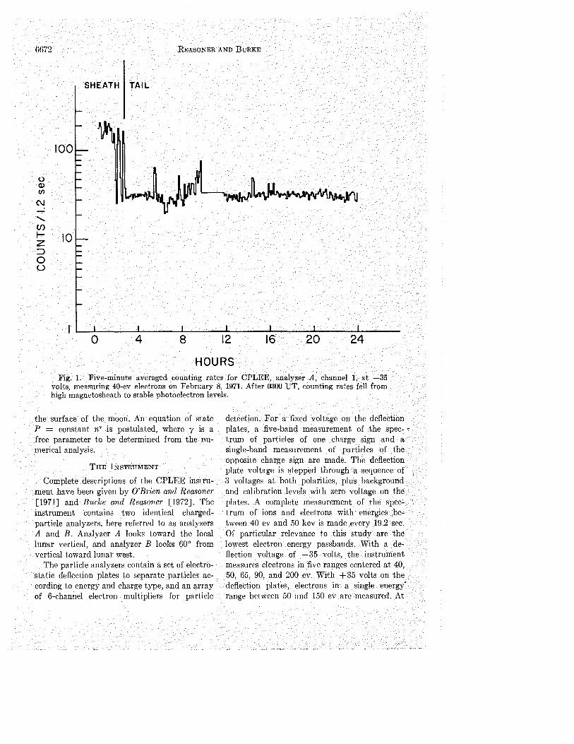
6672 REASONER AND BuRKE

SHEATH TAIL

100

(.) Q) (FJ

C\J

' en I- 10 z ::::> 0 u

0 4 8 12 16 20 24

HOURS Fig. 1. Five-minute averaged counting rates for CPLEE, analyzer A, channel 1, at -35

volts, measuring 40-ev electrons on February 8, 1971. After 0300 UT, counting rates fell from high magnetosheath to stable photoelectron levels.

the surface of the moon. An equation of state P = constant n~ is postulated, where y is a free parameter to be determined from the nu­merical analysis.

THE INSTRUMENT

Complete descriptions of the CPLEE instru­ment have been given by O'Brien and Reasoner [1971] and Burke and Reasoner [1972]. The instrument contains two identical charged­particle analyzers, here referred to as analyzers A and B. Analyzer A looks toward the local lunar vertical, and analyzer B looks 60° from vertical toward lunar west.

The particle analyzers contain a set of electro­static deflection plates to separate particles ac­cording to energy and charge type, and an array of 6-channel electron multipliers for particle

detection. For a fixed voltage on the deflection plates, a five-band measurement of the spec- • trum of particles of one charge sign and a single-band measurement of particles of the opposite charge sign are made. The deflection plate voltage is stepped through a sequence of 3 voltages at both polarities, plus background and calibration levels with zero voltage on the plates. A complete measurement of the spec­trum of ions and electrons with energies be­tween 40 ev and 50 kev is made every 19.2 sec. Of particular relevance to th!s study are the lowest electron energy passbands. With a de­flection voltage of -35 volts, the instrument measures electrons in five ranges centered at 40, 50, 65, 90, and 200 ev. With +35 volts on the deflection plates, electrons in a single energy" range between 50 and 150 ev are measured. At

LUNAR PHOTOELECTRON LAYER 6673

the next higher deflection voltages, ±350 volts, the energy passbands given above are scaled upward by approximately a factor of 10.

OBSERVATIONS

In this sec~ion we present data from the Feb-• ruary 1971 passage of the moon through the

magnetotail. Because these are typical, display of the data from subsequent months would be redundant. At approximately 0300 UT on Feb­ruary ·s, CPLEE passed from the dusk-side magnetosheath into the tail. The 5-min aver­aged counting rates for analyzer A, channel 1, at -35 volts measuring 40-ev electrons, are plotted for this day in Figure 1. Almost identi­cal count rates are observed in analyzers A and B during this period of observation. As CPLEE moves across the magnetopause, the counting

(.) Q) Cl)

•C\1

...... ~en ....

c: :::J 0

(.)

rate drops from -200/cycle to the magnetotail photoelectron background of -35/cycle (1 cycle = 1.2 sec). Enhancements at -0530 hours and at -0930 hours correspond to plasma events associated with substorms on earth [Burke and Reasoner, 1972]. There is a data gap from 1000 to 1200 hours. With the exception of the short­lived (:::; 1 hour) enhancements, the detector shows a stable counting rate when the moon is in the magnetotail.

Our contention is that these stable fluxes ob­served in the magnetotail during periods of low magnetic activity are photoelectrons generated by ultraviolet radiation from the sun striking the surface of the moon. In support of this thesis, we have reproduced the counting rates observed in the same detector on February 10 when the moon was near the center of the tail

0 4 8 12 16 20 24

HOURS Fig. 2. Five-minute averaged deep-tail counting rates of 40-ev electrons on February 10, 1971.

The lunar eclipse (0500 to 0900 UT) is marked by vanishing photoelectron counting rates.

6674 REASONER AND BuRKE

(Figure 2). First, we note that the stable count level is the same at the center as it was when CPLEE first entered the tail. Secondly, from about 0500 to 1000 hours the moon was in eclipse. During this time, the counting rates go to zero. As the moon emerges from the earth's shadow, the counting rates return to their pre­eclipse levels. If the stable low-energy electrons were part of an ambient plasma, rather than photoelectrons, the counting rates would not be so radically altered as the moon moved across the earth's shadow.

A detailed plot of the photoelectron flux on an expanded time scale for the period of lunar entry into the earth's penumbra and umbra is

(/) I 0 103 z

0 >-u 0::

1-w z (/) ILl

(\J ...J <( 0:: ....... m

(/) ~ ._ ::> z z

ILl ::::> Cl. 0 u 10 2 0

ILl 1-::> Cl. ~ 0 (.)

shown in Figure 3. The times of penumbral and umbral entry are indicated, and these times were computed from ephemeris data appropriate to the lunar coordinates of CPLEE. In addition to confirming our earlier arguments, this plot also shows that the high-energy (>40 ev) pho­tons are radiated essentially uniforlnly over the solar disc. If these photons were emitted from a few isolated regions, then one would observe sharp transitions in the flux as the regions were progressively shadowed by the limb of the earth. As can be seen, however, the curve in the penumbral portion is smooth, with no obvi­ous discontinuities. Furthermore, one notices that the counting rate falls by more than 2

>-0:: 1-z ILl

...J <( 0:: m :::IE ::>

0 ILl 1-::> Cl. ~ 0 (.)

10 1

0430 0500 0530 UNIVERSAL TIME

0600 0630

Fig. 3. Expanded time-scale plot of photoelectron fluxes for the period of penumbral and umbral entry of the lunar surface region around CPLEE (analyzer A) during the lunar eclipse of February 10. The data are the counting rate of channel 6 at +35 volts measuring electrons of 50 ev < E < 150 ev.

LUNAR PHOTOELECTRON LAYER 6675

1000 FEB. II FEB.I2

100 (,) Q.) {/)

C\1 -........ en 1-z :::> 0 u

8 12 16 20 0 4

HOURS Fig. 4. An example of ultraviolet contamination of analyzer A from .-1200 of February 11

to .-0300 of February 12, 1971.

orders of magnitude as the moon traverses the umbral and penumbral regions (Figure 3). The

~ minimum counting rate of ,....._ 15/sec for this channel (channel 6) is very near the instru­ment background level, but even if these were all due to an ambient plasma our argument that

, the pre-eclipse counting rates were due entirely to photoelectrons is not significantly altered.

It could be argued that the observed count­ing rates were due to photons scattering within the detectors themselves and not due to ex­ternal photoelectrons. This, however, is not the case. Preflight calibrations with a laboratory ultraviolet source showed enhanced counting rates only when the angle between the look direction of the detector and the source was less than 10°. Given the 60° separation between

•the look directions of analyzers A and B, it would be impossible for the sun, essentially a

point source, to produce identical counting rates in both analyzers simultaneously. There are times when we do observe ultraviolet contami­nation in one or the other channel. An example of such contamination is shown in Figure 4 from 0600 hours, February 11, to 0900 hours, February 12. As the sun moves across the aperture of analyzer A, the counting rates in­crease a full order of magnitude. During this period, analyzer B continued to produce typical deep tail counting rates. Note that as the de­tector came out of .. ultraviolet contamination it encountered typical magnetosheath plasma. At -0345, it passed back into the magnetotail, then at -0800 returned to the magnetosheath.

A typical spectrum of photoelectrons shown in Figure 5 was observed by analyzer A at -0400 hours on February 10, shortly before the moon entered penumbral eclipse. The dark line

6676 REASONER AND BURKE

marks the differential flux equivalent to a back­ground count of one per cycle in each channel (channels 1-5). For all five channels, with the deflection plates at -35 volts, the differential flux is well above this background level. During geomagnetically quiet times, no statistically sig­nificant counts are observed when the deflection plates are at -350 or -3500 volts, correspond­ing to electrons with E > 500 ev [Burke and Reasoner, 1972].

With the exception of periods of ultraviolet contamination in analyzer A, we always ob­serve nearly the same counting rate due to photoelectrons in analyzers A and B. For all purposes, we can say that the spectrum dis­played in Figure 5 is just as typical for ana­lyzer B. We have found no case of anisotropy in the photoelectron fluxes. In all cases, too, we found that the photoelectron spectra observed in both analyzers had close to a power-law de­pendence on energy. If we write the differential flux in the form j(E) = io(E/E.t", fl. is between 3.5 and 4. In the next section, the details of this spectrum are more carefully studied.

Also in Figure 5 we display a schematic cross section of our instrument as it is deployed on the surface of the moon. The apertures of both

> ., ~ ., -

~ "' I

(J ., Ul

N~ (J

...... Ul c: ~ (J ., ~

X ::;) ...J u.

idL--r~OTrrrr--~-nnnnr~-rrn~r-,--101

ENERGY Fig. 5. Typical photoelectron spectrum ob­

served by CPLEE at the lunar surface in the high­latitude magnetotail.

analyzers are elevated 26 em from ground. Their geometry is such that they observe only electrons with a component of velocity in the downward direction. Since we continually ob­serve photoelectrons with energies up to -200 ev, we must assume that the lunar surface po­tential iR at least 200 volts during these times. This measurement will seem high to those familiar with the work of E. Walbridge (un­published manuscript, 1970) and Grobman and Blank [1969], who calculate a surface potential that is at least an order of magnitude lower. The difference is that their models deal with photoemissions from the surface of the moon in the presence of the solar wind. Our measure­ments in the magnetotail are made under near­vacuum conditions. After further analysis of the problem, we return to considerations of the surface potential.

To summarize: During geomagnetically quiet times, when the moon is in the magnetotail and not in eclipse, stable photoelectron fluxes with energies between 40 and 200 ev are observed. These fluxes are isotropic and obey a power law, E-", where JL is between 3.5 and 4. From the fact that CPLEE is observing downward­moving electrons, we conclude that in the mag­netotail the lunar surface potential is of the order of 200 volts.

A FIYDROSTATIC 110DEL

Our observation of steady photoelectron fluxes that are isotropic over the lower half­plane for much of the moon's passage through the magnetotail suggests that we can make the following assumptions about the physical situa­tion:

1. The solar radiation flux at the lunar surface and the photoelectron flux produced by the lunar surface are constant in time.

2. There are equal probabilities for emitting photoelectrons into equal solid-angle elements in the upper half-plane.

3. In the equilibrium situation, the net cur­rent out of the surface is zero.

4. The lunar surface may be approximated by a flat infinite plane. Physical quantities vary only with height above the surface. (The co­ordinate system is such that X, Y, Z increase toward the local vertical, west, and south, • respectively.)

LuNAR PHoTOELECTRON LAYER 6677

The first assumption assures a constant flux of photoelectrons at the surface of the moon. In the Appendix, we show that our postulate of an isotropic production of photoelectrons is sufficient to explain our observation of isotropic fluxes at 26 em. Assumption 3 demands that in a vacuum all photoelectrons be trapped by the electrostatic field above the surface. The surface potential under vacuum conditions is deter­mined by the most energetic photoelectrons.

In the equilibrium situation, the governing equations are Poisson's equation,

(1)

and the equation of conservation of momentum,

q acp(x) = + _1_ aP(x) (2) ax n(x) ax

Here the density and pressure are defined by

n(x) = J f(v, x) d3v

The density can be eliminated from equations 1 and 2 to show that

P(x) = _!__ (acp(x2)2 871" ax

However, to solve for all three quantities we must postulate an equation of state

P(x) Po --=-=a n7 (x) no7

(3)

where a is a constant, and y is related to the polytrope index v by the relationship y = ( v

+ 1)/v. The values of physical quantities at the surface are denoted by zero subscripts. In solv­ing equations 1-3, we demand that, as x -c> oo, all physical quantities go to zero.

Pressure can b~ eliminated by differentiating equation 3 and substituting into 2:

acp = + ')Ia n-y-2 dn ax q dx

(4)

If we multiply (1) by .acp;ax, using (4) on the right-hand side, and integrate in from infinity, we get

l oo ( ) 7 _ 1 dn(x') = -87r')'a n x' --,- dx'

x dx (5)

acp(xl = ±[8m:m"(x)Jl/2 ax

In order to insure a potential that decreases as x increases, we must choose the minus sign in equation 5. Equating the right-hand sides of equations 4 and 5,

or

-x = J::: E!._ n<" 12>- 2 dn ( )

1/2 fn(x) q 81r no

For y =j=. 2,

n(x) = no [ 1 - 'Y ~ ~ ~JI<"Y-2

> (6a)

and for y = 2

n(x)

with the characteristic length

(6b)

Equations 6a and 6b can be substituted into 4 to get:

cf>o _ cp(x) = 2P0

"Aqno

. f ( 1 - :r_ ~ ~ ~r/(")'-2) dx (7a)

'Y ~ 2

'Y = 2 For y =j=. 2 (equation 7 a), there are two

formal solutions, depending on whether y = 1 or not:

- __ .f§L __ cf>o - cp(x) - qno('Y - 1)

.[ 1 - { 1 - 'Y ~ 2 ~r")'-1)/")'-2

] (7a')

'Y ~ 1, 2

6678 REASONER AND BuRKE

<Po - <P(x) = 2Po In (1 + :!::)

qno A (7 a")

'Y = 1

The solutions for the electrostatic potential, equations 7a', 7a", and 7b, satisfy the boundary conditions cp ( 0) = cpn ::::::: 200 volts and cp ( oo ) = 0. Here cp0 = (Po/qn 0 )y/(y - 1). If 1 < y ::::; 2, cp(x) goes smoothly to zero as x ~ oo. If y > 2, cp(x) goes to zero at x = A,y/(y- 2). However, of 0 < y < 1, both boundary con­ditions cannot be satisfied for finite <Po· It would be possible to have an equation of state with finite <Po and y ::::; 1 near the surface, but the value of y must shift to a value greater than 1 beyond some height. The numerical analysis of the following section shows that this is the case.

NuMERICAL ANALYSIS

General theory. The variations of photoelec­tron density and electrostatic potential above the surface of the moon can be calculated nu­merically. Again we approximate the lunar sur­face by an infinite plane, with the x direction normal to the surface, and assume spatial varia­tions of physical quantities only with the height.

At a height x above the surface, the electron density is f f(v, x) d'v, where f(v, x) is the elec­tron distribution function. If we assume an isotropic flux at the surface, the Liouville theorem can be used to show that the distribu­tion function is independent of angles at all heights. Writing

d~v = (2E/ m3)

112 dE dQ

and integrating over solid angles, we obtain for the density

Since the distribution function is a constant along particle trajectories, f(E, x) = f(E., x = 0), where E =Eo- q[</>o- <f>(x)]. By chang­ing the variable of integration from E to E., equation 8 can be expressed

n(x) = 411"

·fro {2m(E0 - q[c/>0 - <P(x)])} 112

q[<f>o-<f>(x)]

· f(Eo, X ~ 0) dEo (9)

To calculate the distribution function of photoelectrons at the surface, we consider the quantity

j(E0) dEo

= [J: I(hv) Y(hv)p(E0 , hv) dhv] dE0 (10)

the upward-moving flux of photoelectrons emitted from the surface with energies between E. and E. + dE., where I(hv)d(hv) is the flux of photons reaching the lunar surface with energies between hv and hv + d(hv). The quantum yield function Y (hv) gives the num­ber of electrons emitted by the surface per in­cident photon with energy hv, and p(E., hv )dE. is the probability that an electron emitted from the surface, due to a photon with energy hv, will have a kinetic energy between E. and E. + dE •. The quantity p (En, hv) is normalized so that

L" p(E0 , hv) dE0 1

W is the work function of tlie lunar surface material.

The total upward-moving flux at the surface is S,p(x = 0) = f.ooj(E.)dE •. But

Sup(X = 0)

12.-

1.-/2 fro

= 0 0 0 Vof(Eo, e, <P, O)vo2

dvo

· i sin e dO de/>

Since Vo = Vo[i cos e + j sin e cos <P + k sin e sin <Pl and f is independent of angle,

1ro2E = 7r

0 -;;,~ f(Eo, X 0) dE0 (11)

Thus

f(Eo, X 0) (12)

n(x) = 2

·fro {2m(E0 - q[<Po- cf>(x)])} 112

q[<f>o-</>(x}]

_j(Eo) dE0

(13) Eo

LuNAR PHOTOELECTRON LAYER 6679

The potential as a function of height is evaluated by multiplying Poisson's equation, a"cp/8x' = -47Tqn(x), by 8cf>/8x and integrating in from x =, ciJ to get

(ocf>/ox) 2 =_ -81rq 1° n(<P') ckp' (14) </>(x)

where we have written

1"' n(x')(ocf>/ox') dx' = 1° n(<P') ckp' x </>(x)

A further integration out from the surface gives us the potential at a point x.

Computational methods and results. To de­termine the upward-moving differential flux at the surface, upon which the distribution func­tion, number density, and potential depend, we must first calculate the integral in equation 10. The solar photon differential flux at 1 AU, l(hv), is taken from Friedman [1963] for the range 2000 to 1800 A and from Hinteregger et al. [1965] for the range 1775 to 1 A and is plotted in Figure 6. Following the suggestion of Walbridge [1970], we have:

1016

1015

io14

1013

> 16'2 w ' u

w 1011 (/)

' "' ::i: u lo!O ...... (/) z 0

109

f-0 :c a.

108

107

106 0 40 80

1. Adopted a work function of lunar ma­terial of 6 ev.

2. Assumed a photoelectron yield fui1ction of the form

Y(hv) 0 hv < 6 ev

Y(hv) hv- 6

6 < hv < y --- 9 ev 0 3

Y(hv) = Yo hv > 9 ev (15)

where Y. is a free parameter of our calculation. 3. Chosen a probability function

p(E, hv) = 6E(E1 - E)/E1 0 ::; E ::; E1

(16)

p(E, hv)

where

0

hv- TV

0

E > E 1

hv 2:: TV

hv < W

In general, the probability function IS a

120 160 200 240 280

PHOTON ENERGY ( EV)

Fig. 6. Solar photon energy spectrum at 1 AU from 2000 to 1 A~

6680 REASONER AND BURKE

complicated function depending on the nature of the photoemission material. However, Grab­man and Blank [1969] have shown that for the purpose of calculating equation 10 any broad function with zeros at E = 0 and E = E, and a width f!.E ,...., hv will suffice. A plot of p(E, hv) is shown in Figure 7 for various values of E,.

The upward-directed .differential flux in elec­trons/cm2 sec ster ev for the values Yo = 1, 0.1, 0.01 were numerically computed and have been plotted in Figure 8. We have also inserted the photoelectron differential flux observed by CPLEE at 26 em. The Liouville theorem allows us to set a lower bound on Yo of 0.1. That is, if there were no potential difference between the ground and 26 em, the yield function would be 0.1 electrons/photon. After estimating the potential difference between 26 em and ground, we can also determine an upper bound on Y 0 •

Solving the integra-differential equation 14 for <P (x) involves an integration from the sur­face outward, with an assumed value of <Po· However, the expression for iJcpjiJx involves an integral from infinity in to x, or equivalently from cp = 0 to cp(x). By the expedient of divid­ing the integral into pieces in Eo space and using an analytic approximation to the func­tion j(Eo) in each of these intervals, a solution

was effected. In this way, it was only necessary to know the values of <P = </J(x) and cp =. 0 at the end points of the interval, and the solution would proceed. In Figure 9 we show families of solutions for cp(x) with several values of the parameter Yo.

The value of Yo calculated by assuming no potential difference between the surface and x = 26 em was 0.1. Figure 9 shows that, for Yo = 0.1, the potential difference <P ( x = 0) -cp(x = 26 em) is only 3 volts. Obviously, we could now use an iterative procedure, modifying our spectral measurement at 26 em to obtain the surface spectrum according to the equation f(E, x) = f(Eo, 0) and hence obtain a new estimate of Y.. However, the procedure is hardly justified considering the small potential difference ( ,....,3 volts) and the energy range of the measured photoelectrons ( 40 to 200 ev). Hence from our measured photoelectron fluxes and numerical analysis we obtain a lunar sur­face potential of at least 200 volts and a value of the average photoelectron yield of Yo = 0.1 electrons/photon.

LUNAR SuRFACE PoTENTIAL cp 0

The presence of photoelectrons at 200 ev without significant fluxes in the next highest energy channel at 500 ev leads us to conclude that the lunar surface potential is at least 200

.07~---r----.---~---.----.---~----.----.----.---·

E (ev)

Fig. 7. Probability function that a photon of energy hv will cause the lunar surface material to emit a photoelectron of energy E, with different values of E, = hv- W.

LUNAR PHOTOELECTRON LAYER 6681

> Q) I

u Q)

"' I C\1 E ~ c: e -u Q)

~ X

108 ::::> ...J u.. z 0

107 a:: 1-frl ...J UJ g 0 :X: a. UJ u ~ a:: ::::> (/)

103 1o·2 103

ENERGY (EV)

Fig. 8. Numerically computed photoelectron spectra emitted for the yield functions Yo = 1, 0.1, and O.Dl electrons per photon. The photo­electron spectrum measured by CPLEE (shown by plus signs) is found to fall close to the Yo = O.lline.

volts. The data of Hinteregger et al. [1965] show significant solar photon fluxes up to 400 ev, and presumably the lunar surface potential

,. under vacuum conditions could be 400 volts. However, we detected no photoelectrons with E > 400 ev, although it should be noted that the extrapolation of our measured spectrum (Figure 5) to 400 ev is below the instrument background. We have therefore adopted a con­servative value of 200 volts as the lunar surface potential for the calculations in the preceding and following sections.

The lunar surface potential can be decreased, however, by the presence of a hot ambient plasma that furnishes an electron return cur­rent that partially balances the emitted photo­electron current. In effect, the highest-energy photoelectrons can escape from the potential

• well, since electrons from the ambient plasma furnish the return current to balance these

('SCaping photoelectrons. Quantitativdy, if F, is the net negative flux to the lunar surface from the ambient plasma, and j(Eo) is the emitted photoelectron ('nerg~· spectrum in units of electrons jcm' S('C ('V, th('n

F., = fro j(Eo) dE" q¢,

(17)

and this equation can be solwd for cpo, the lunar surfac(' pot('ntial.

Our measurements of 11hotoelectrons W('re tak('n during periods in the magnetotail when all the channels of the in~trument exc('pt the lowest-energy electron channels were at back­ground levels. Thus we can establish an upper limit to the electron flux from the ambient plasma for electrons with 40 ev < E < 50 kev. Figure 5 shmvs the 'background spectrum,' calculated by conv('rting the background count­ing rate of ,_, 1 count/sec to equivalent flux in each of the energy channels. Integrating over this spectrum and converting to flux over the h('misphere gives F,. :s; 3.4 X 10" electrons/em' sec. We feel that this is a valid upper limit, as the range of measurement in ('nergy includes the peak energ~- of the plasma-sheet spectrum (--- 1 kev).

We note that Vasyliunas [1968] obtained an upper limit to the electron concentration for

180o~--~,0----2~0----3~0----40~--~50~--~60--~70

HEIGHT (CM)

Fig. 9. Numerically eomputed potential dis­tribution above the lunar surface for several val­ues of the yield function Yo. For Yo = 0.1, the potential difference between ground and 26 em is about 3 volts.

6682 REASONER AND BURKE

locations outside the plasma sheet based on Ogo 3 data. The relation expressed was NEo112 < 10-2 em-a kev11 2, where N is the electron density, and Eo is the energy at the peak of the spectrum. For an isotropic plasma in which the bulk motion can be neglected relative to the thermal motion, the electron flux to a probe is given by F, = Nv/2(7T-)1". Applying the appropriate con­version factors, the expression of Vasyliunas results in an upper limit to the electron flux of F, < 5.6 X 107 electrons/em' sec.

The emitted photoelectron energy spectrum j(E .. ) is shown in Figure 8. The procedure involved in calculating the surface potential ¢o is to integrate the function j(E) from the maxi­mum energy of 200 ev backward until the total flux is equal to the upper limit of the return flux. The computation was done for Yo = 1, 0.1, and 0.01, and for the two values of the upper limit of the return flux derived above. The results are shown in Table 1.

The lower half-height of the channel 5 energy passband is 160 ev. Hence the surface potential could be as low as 160 volts and still result in particle fluxes in channel 5. This estimate of the potential is seen to be not inconsistent with values of Y. = 0.1 and F, ~ 3.4 X 10", result­ing in a surface potential (Table 1) of 114 volts.

One rather obvious prediction of our argu­ments about the surface potential is that, when the electron flux reaching the surface of the moon is high enough, surface-generated photo­electrons with energies in the range of our de­tector should vanish. This happens in the solar wind and magnetosheath, but it is impossible for CPLEE to provide conclusive observational evidence in the presence of contamination by solar wind and magnetosheath electrons that the >40-ev photoelectrons are not returning to the surface and hence entering the detectors. Electron densities > 1 cm-3 and temperatures

TABLE 1. Lunar Surface Potential

Electron Flnx Yo <Po, volts

3.4 X 106 1.0 181 3.4 X 106 0.1 114 3.4 X 106 0.01 44

5.6 X 107 1.0 96 .5.6 X 107 0.1 36 5.6 X 107 0.01 8

,_, 15 ev, such as those commonly encountered in the solar wind and magnetosheath, provide much higher fluxes in the 40- to 200-ev range than photoelectron fluxes observed in the high­latitude magnetotail.

On April 9, 1971, a worldwide magnetic storm was observed by CPLEE [Burke et al., 1972] in which the magnetosheath moved in to YsE = 15 RE. As the magnetopause moved out past the moon, intense plasma-sheet fluxes were ob­served. At this time, the fluxes observed in the 40-, 50-, and 70-ev channels fell bf'low photo­electron levels. In Figure lO(a) we show the count rates for the 40-ev and .500-ev electron channels from 1100 to 1200 UT on April 9. A heavy line has been drawn at the 40-ev photo­electron level. As the 500-ev count rate rises, the 40-ev count rate falls below this line. From 1128 to 1135 UT, when the 500-ev count rate dropped, the 40-ev channel returned to the photoelectron level. In Figure 10 (b), we have plotted the electron spectra at 1110 (plasma sheet) and at 1135 (photoelectron). The inte­gral flux at 1110 was calculated to be 2.5 X 10' cm-2 sec-1

• Such a flux reduces the surface potential to less than 10 volts. Thus we are observing a modulation of the surface potential by plasma-sheet fluxes into the lunar surface.

DISCUSSION

For the sake of comparison with the predic­tions of the hydrostatic model, we have plotted the numerically calculated density, pressure, and potential difference from x = 0 out to a height of 200 meters in Figure 11. In Figure 12 the pressure is plotted as a function of num- " ber density to obtain the equation of state. We find that, from 0 < x ~ 30 em, the value of y is about 0.5. From 30 to 100 em, y drops to a value of 0.2, then recovers to about 0.5 out to x = 2000 em. Beyond this point, y shifts toward a value greater than 1.

The dashed lines in Figure 11 represent the density and potential difference as computed from equations 6a and 7a' u;;ing y = 0.5. A surface pressure of --2 x w-' erg/ em" and density --6 X 10' em-" give a value of A. = 2.1 em. Out to x = 200 em, the numerically calculated potential agref's quite well with the h~·drostatic prediction. Beyond this height, the potential difference rises less steeply than the " y = 0.5 prediction. However, this can be under-

LUNAR PHOTOELECTRON LAYER 6683

N 0

40ev.

(b)

u 411 Cll

<'! ...... (/) 1-z :::;)

0 u

> w I -Q

0:: w 1-(/) I

u w (/) I

500ev. N N

0

0

0 0+--..-~-r-"-.u,.--.---1

II 12

::liE u ...... (/)

w ...J u 1-0::

~ X :::;) ...J L&..

102

10 1

Fig. 10. (a) Counting rates for the 40-ev and 500-ev channels between 1100 and 1200 UT, April 9, 1971. (b) Electron spectra observed at 1110 and 1135 UT, showing plasma-sheet and photoelectron fluxes.

stood in terms of the shift to larger than unity values of y required by equation 70: if the boundary condition cp( oo) = 0 is to be met.

The density curve is much more sensitive to fluctuations in the value of y. The variations in the region 30 ~ x ~ 300 em correspond to potential differences of 3 to 15 volts from ground. We note that in Figure 8 the photo­electron flux generated at the surface has sharp breaks in this region. Evidently the photoelec­trons can be broken up into three groups of low (0 < E ~ 1 ev), medium (1 < E < 10 ev), and high (10 < E < 200 ev) energy. Where one distribution dominates over the others, a value of y is established. Fluctuations in y are found in the transition regions between populations.

Feuerbacher et al. [1972] have measured the photoelectron yield of a lunar fine sample. In the photon energy range 5 < E < 20 ev, they

• found a yield function that reaches a maximum value of .-0.08 at 15 ev, then drops to 0.01

Fig. 11. Numerically computed values of elec­tron density, potential difference, and pressure as a function of distance from the lunar surface. The dashed line represents a 0.5 power-law curve.

6684 REASONER AND BuRKE

"'E u ' 1/) 169

~ 2 w a::: ~ 1610 (j)

w a::: a_

1011

DENSITY (ELECTRONS/cm3 )

Fig. 12. Plot of photm~lectron pressure against density to determine the local equation of state.

at 20 ev. B. Fitton (private communication, 1971) has suggested that our value of 0.1 is more a measurement of the CPLEE instrument case yield function than that of the lunar sur­face. We find it difficult to understand how this could be the case.

First, were CPLEE an electrically isolated package, the requirement that the net current to the instrumE'nt be zero would result in a measured yield function that is representative of the case material. Relative to the lunar sur­facE', the case would bear a positive potential in order to maintain an enhanced photoelectron dE'nsity in its immediate vicinity.

The fact is, however, that CPLEE is not electrically isolated. CPLEE is connected to the central Alsep station. Further, at any given time, only the top surfaces and one or two sides of Alsrp packages are illuminated by the sun, while the remaining area is shadowed. These unilluminated surfaces provide receptor areas for return current from the photoelectron gas. Thus no large potential difference can develop between CPLEE and the lunar surface, and photoelectrons emitted at the lunar surface and at the CPLEE case are indistinguishable. Geometrical considerations of electron trajec-

tories would lead us to expect that the bulk of the photoelectrons measured by CPLEE were emitted at the lunar surface at least several meters from CPLEE. If the Alsep instrument cases had a photoelectron yield much larger or much smaller than the yield of the lunar sur­face, then one would expect a perturbation of the photoelectron flux in the vicinity of Alsep. This perturbation would depend not only on the ratio of photoelectron yield, but, more impor­tant, on the ratio of the area of the Alsep in­struments to the area encompassed by the tra­jectories of E > 40 ev photoelectrons from a point source. This last area is of the order of the square of the scale height of photoelectrons with E > 40 ev ( ,._, 10 meters, Figure 11). Since the Alsep area is ,..,3 m2

, the ratio of areas is of the order of 2%. Thus, even if the yield of the instrument cases were a factor of 10 greater or smaller than the surface yield, the flux per­turbation would only be 20%.

Second, were CPLEE measuring its own photoelectrons, one would expect to observe changes in the relative fluxes observed in the two analyzers with solar zenith angle as the electron cloud surrounding the instrument ad- '" justs to changing illumination. Specifically, the

LUNAR PHOTOELECTRON LAYER 6685

ratio of the flux observed by analyzer B (look­ing 60° west of vertical) to the flux observed in analyzer A (looking to the vertical) should be

, larger after lunar noon than before. Our data show isotropic photoelectron fluxes across the entire magnetotail.

SUMMARY AND CONCLUSIONS

In this paper, we have reported the obser­vation of stable, isotropic photoelectron fluxes 26 em above the lunar surface. In the energy range 40 ::::; E ::::; 200, the flux obeys a power law of the form j(E) = j,(EjE,)-", where p. is between 3.5 and 4. Because these fluxes were moving down, we conclude that, in the near­vacuum conditions of the high-latitude mag­netotail, the lunar surface potential is at least 200 volts. The modulation of the surface po­tential in the presence of intense plasma-sheet fluxes has also been observed. It was shown that these electrons can be explained in terms of the measured solar photon spectrum produc­ing an isotropic flux of photoelectrons at the surface. A photoelectron yield function of Y, = 0.1 electron/photon was calculated. Finally, we have shown that the numerically calculated pressure, density, and potential distributions can be approximated by the solutions to a set of hydrostatic equations that employ an equation of state P /n'12 = constant out to 200 em from the surface. Beyond this height, the equation of state shifts toward the isothermal case, P jn

• = constant.

APPENDIX

Here we present a justification for using a scalar pressure in the equation of state ( equa­tion 3).

By definition, the number density, flux, and pressure are

n(x) = I f(v, x) d3v

= f N(E, !1, X) dE dQ

S(x) = J vf(v, x) d3v

(A1)

f vS(E, !J, X) dE dQ

P(x) = J mvvf(v, x) d3v

= f vvP(E, Q, X) dE dQ

Here we have used d"v = '' 2nv sin (} d(J dcp (2Ejm")'12dE dn and have cknned the direc­tional differential density, flux, and pressure

(2E) 11

2

N(E, !J, X) == m~ f(E, Q, X)

S(E, !1, X) == 2~ f(E, n, X) (A2) m

" ( 2E)a;2 P(E, !J, X) == --;;; f(E, !J, X)

The angular dependence of these quantities is contained only in the distribution function. To compare one of the directional differential quantities at a point X, with its value at the ground, X = 0, we usc the Lionville theorem:

t~(El, !11, X1) = foCEo, !lo, Xo)

The distribution function is a constant along particle trajectories. Subscripts 0 and 1 indi­cate the value of the quantity at x = 0 and an arbitrary height x = X,.

In our model, we assumed an isotropic photo­electron production (at X = 0) over the upper half-plane in velocity space. Since all electrons are trapped in a conservative field, isotropy is maintained over the whole of velocity space at X = 0. Thus f, is independent of n,. From the conservation of energy

or

/JCE1, !11, X1)

= fo(E1 + q[c/>o - c/>(X1)] (A3)

Thus if photoelectrons are isotropic at the ground, they are isotropic at X,. This explains our observation of isotropic fluxes, measured at X = 26 em. In this case, the directional dif­ferential pressure is also isotropic, and on inte­gration reduces to the scalar form used in the text.

Being independent of angle, the distribution function is an even function about Vx = 0, v, = 0, and Vz = 0. The Vlasov equation

6686 REASONER AND BURKE

at + v at _ .!!_ acp jj_ = 0 at X ax max avX

has nontrivial moment solutions only when multiplied by VxVx", Vxv:, or Vxvz". These mo­ment equations take the form

a 2 earp· -a n(x)( V (x)) + --a n(x)

X m X 0 (A4)

and

3e acp 2 + --a n(x)(vx (x)) m x

0

a~ n(vx2(x)v.

2(x)) (A.5)

+ .!!_ aacp n(x)(vx2(x)) m x

0

0

where

n(x)(v/(x)) = J d3vv/f(v, x)

Since the distribution function depends only on velocity, equations (A4) and (A5) can be written

0 (A4')

a 5e acp -a I6(x) + --a l 4(x) X m X

0 · (A5')

where

l2,(x) = iro v2't(v, x) dv

If, for example, we had a locally Maxwellian gas

( ) n(x) -v' /w' (x)

tv, x = 11"3!2w3(x) e

then

(2v - 1)! !n(x)w2'-

2(x) 2'+111"

and (A4') becomes

an(x)w2(x) + 2e acp n(x)

ax max 0

and (A5'),

an(x)w4(x) + 2e acp n(x)ul

ax max 0

Expanding, we get

w2(x)[an(x)w4

(x) + 2e acp n(x)J ax max

+ 7J(x)w2(x) aw2(x) = 0 ax

Since the bracketed term is zero and n(x)w2 (X) > 0, w•(x) is a constant. This is the isothermal case, whose solution n(x) = m0 exp { -q[cp. - cp(x)]/mw2

} is well known. In general, however, (A4') and (A5') cannot

be solved without assuming a distribution func­tion, from which the equation of state can be determined from (A5').

Acknowledgments. This work was supported by National Aeronautics and Space Administra­tion contract NAS9-5884.

* * * The Editor wishes to thank V. M. Vasyliunas

and E. C. Whipple for their assistance in evalu·· ating this paper.

REFERENCES

Burke, W. J., and D. L. Reasoner, Absence of the ., plasma sheet at lunar distance during geomag­netically quiet times, Planet. Space Sci., 20, 429, 1972.

Burke, W. J., F. J. Rich, D. L. Reasoner, D. S. • Colburn, and B. E. Goldstein, Effects on the geomagnetic tail at 60 RE of the worldwide storm of April 9, 1972, submitted to J, Geophys. Res., 1972.

Feuerbacher, ·B., M. Anderegg, B. Fitton, L, D. Laude, and R. F. Willis, Photoemission from lunar surface fines, in Lunar Science, val. 3, edited by C. Watkins, pp. 253-255, Lunar Sci. Inst., Houston, Tex., 1972.

Friedman, H., Rocket spectroscopy, in Space Sci­ence, edited by D. P. LeGallet, p. 549, John Wiley, New York, 1963.

Grohman, W. D., and J. L. Blank, Electrostatic potential distribution of sunlit lunar surface, J. Geophys. Res., 7 4, 3943, 1969.

Guernsey, R. L., and J. H. M. Fu, Potential dis­tribution surrounding a photo-emitting platein a dilute plasma, J. Geophys. Res., 75, 3193, 1970. •

Hinteregger, H. E., L. A. Hall, and G. Schmidtke,

..

LUNAR PHOTOELECTRON LAYER 6687 Solar XUV radiation and neutral particle distri­bution in July 1965 thermosphere, in Space Res., 5, 1175-1190, 1965.

Medved, D. B., On the formation of satellite electron sheaths resulting from secondary emis­sion and photoeffects, in Interaction of Space Vehicles with an Ionized Atmosphere, edited by S. F. Singer, p. 305, Pergamon, New York, 1968.

O'Brien, B. J., and D. L. Reasoner, Charged par-

ticle lunar environment experiment, Apollo 14 Preliminary Science Report, NASA Spec. Publ. 272, 193, 1971.

Vasyliunas, V. M., A survey of low-energy elec­trons in the evening sector of the magneto­sphere with Ogo 1 and Ogo 3, J. Geophys. Res., 73, 2839, 1968.

(Received June 6, 1972; accepted August 1, 1972.)

MEASUREMENT OF THE LUNAR PHOTOELECTRON

LAYER IN THE GEOMAGNETIC TAIL

DAVID L. REASONER and WILLIAM J. BURKE

Dept. of Space Science, Rice University, Houston, Tex. 77001, U.S.A.

Abstract. The Charged Particle Lunar Environment Experiment (CPLEE), a part of the Apollo 14 ALSEP, is an ion-electron spectrometer capable of measuring ions and electrons with energies between 40 eV and 50 keY. The instrument, with apertures 26 em above the surface, has detected a photo­electron gas layer above the sunlit lunar surface, with energies ranging up to 200 eV. Experimental data for periods while the Moon was in the Earth's magnetotail for electrons with energies 40 eV ~ E~ 200 eV follow a power law spectrumj (E)= jo(E/Eo)-'" with 3.5 ~ ,u ~ 4. In the absence of photoelectrons with E > 200 eV, we assume that the surface potential is at least 200 V. The modulation of this potential in the presence of intense plasma sheet fluxes has been observed.

Numerical solutions for the variation of electron density and potential as functions of height above the lunar surface were obtained. The solar photon spectrum I (hv), obtained from various experi­mental sources, and the photoelectron yield function of the surface materials, Y (hv), are two para­meters of the solution. Energy spectra at the height of the measurements for various values of Y (hv) were computed until a fit to experimental data was obtained. Using a functional form Y (hv) =

=[Yo(hv-W)]/(W/2) for 6eV;;;;hv;;;;9eV and Y(hv)=Yo for (hv)>9eV where W,thelunar surface work function, was set at 6 eV, we calculated a value of Yo= 0.1 electrons photon-1 . The solution also showed that the photoelectron density falls by 5 orders of magnitude within 10 m of the surface, but the layer actually terminates several hundred meters above this height.

1. Introduction

The general problems of photoelectron emission by an isolated body in a vacuum and in a plasma have been the objects of several investigations. For example, Medved (1968) has treated electron sheath formations about bodies of typical satellite dimen­sions. Guernsey and Fu (1970) have considered the properties of an infinite, photo­emitting plate immersed in a dilute plasma. Grohman and Blank (1969) obtained expressions for the lunar surface potential due to photoelectron emission while the moon is in the solar wind. Walbridge (1970) developed a set of equations for obtaining the density of photoelectrons as well as the electrostatic potential as functions of height above the surface of the Moon while the Moon is in the solar wind. By assuming a simplified form of the solar photon emission spectrum he could provide analytic expressions for these quantities.

In this paper we report on observations of stable photoelectron fluxes, with energies between 40 and 200 eV by the Apollo XIV Charged Particle Lunar Environment Experiment (CPLEE). These observations, made in the magnetotail under near vacuum conditions, are compared with numerically calculated photoemission spectra to determine the approximate potential difference between ground and CPLEE's apertures (26 em). Numerically calculated density and potential distributions, when compared with our measured values, help us estimate the photoelectron yield function of the dust layer covering the Moon.

R. J. L. Grard (ed.), Photon and Particle Interactions with Surfaces in Space, 369-387. All Rights Reserved Copyright © 1973 by D. Reidel Publishing Company, Dm·drecht-Hol/and

370 D.L.REASONER AND W.J.BURKE

2. The Instrument

Complete descriptions of the CPLEE instrument has been given by O'Brien and Reasoner (I 971) and Burke and Reasoner (1972). The instrument contains two identical charged-particle analyzers, hereafter referred to as analyzers A and B. Analyzer A looks toward the local lunar vertical, and analyzer B looks 60° from vertical toward lunar west.

The particle analyzers contain a set of electrostatic deflection plates to separate particles according to energy and charge type, and an array of 6 channel electron multipliers for particle detection. For a fixed voltage on the deflection plates, a five band measurement of the spectrum of particles of one charge sign and a single-band measurement of particles of the opposite charge sign are made. The deflection plate voltage is stepped through a sequence of 3 voltages at both polarities, plus background and calibration levels with zero voltage on the plates. A complete measurement of the spectrum of ions and electrons with energies between 40 eV and 50 keV is made every 19.2 s. Of particular relevance to this study are the lowest electron energy pass bands. With a deflection voltage of -35 V, the instrument measures electrons in five ranges centered at 40, 50, 65, 90 and 200 eV. With + 35 Von the deflection plates, electrons in a single energy range between 50 and 150 eV are measured. At the next higher deflection voltages of± 350 V, the energy pass bands given above are scaled upward by approximately a factor of 10.

3. Observations

In this section we present data from the February 1971 passage of the moon through the magnetotail. Because these are so typical, the display of data from subsequent months would be redundant. At approximately 0300 UT on February 8 CPLEE passed from the dusk side magnetosheath into the tail. The five minute averaged counting rates for analyzer A, channel I, at -35 V measuring 40 eV electrons are plotted for this day in Figure I. Almost identical count rates are observed in analyzers A and B during this period of observation. As CPLEE moves across the magnetopause the counting rate drops from ~ 200 cycle -t to the magnetotail photoelectron back­ground of~ 35 cycle- 1 (1 cycle= 1.2 s). Enhancements at ~0530 hand at ~0930 h correspond to plasma events associated with substorms on Earth (Burke and Reasoner, 1972). There is a data gap from 1000 to 1200 h. With the exception of the short lived (::::; 1 h) enhancements the detector shows a stable counting rate when the Moon is in the magnetotail.

Our contention is that these stable fluxes observed in the magnetotail during periods of low magnetic activity are photoelectrons generated by ultraviolet radiation from the Sun striking the surface of the Moon. In support of this thesis we have reproduced the counting rates observed in the same detector on February 10 when the Moon was near the center of the tail (Figure 2). First, we note that the stable count level is the same at the center as it was when CPLEE first entered the tail. Secondly, from about 0500 to 1000 h the Moon was in eclipse. During this time we observe the

(.) Q) If)

N .

....... (J)

1-z ::)

0 u

THE LUNAR PHOTOELECTRON LAYER IN THE GEOMAGNETIC TAIL

SHEATH TAIL

0 4 8 12

HOURS

16 20 24

371

Fig. 1. 5-min averaged counting rates for CPLEE, analyzer A, channel I at -35 V, measuring 40 eV electrons on February 8, 1971. After 0300 UT counting rates fell from high magnetosheath

to stable photoelectron levels.

100

(.)

Q)

"' N

.......

"' 10 +-c:: ::3 0 u

0 4 8 12 16 20 24

HOURS

Fig. 2. 5-min averaged deep tail counting rates of 40 eV electrons on February 10, 1971. The lunar eclipse (0500-0900 UT) is marked by vanishing photoelectron counting rates.

372 D.L.REASONER AND W.J.BURKE

counting rates go to zero. As the moon emerges from the Earth's shadow, the counting rates return to their pre-eclipse levels. If the stable low energy electrons were part of an ambient plasma, rather than photoelectrons, the counting rates would not be so radically altered as the moon moved across the Earth's shadow.

It could be argued that the observed counting rates were due to photons scattering within the detectors themselves and not due to external photoelectrons. This however is not the case. Preflight calibrations with a laboratory ultraviolet source showed enhanced counting rates only when the angle between the look direction of the detector and the source was less than 10°. Given the 60° separation between the look directions of analyzers A and B, it would be impossible for the Sun, essentially a point source, to produce identical counting rates in both analyzers simultaneously.

A typical spectrum of photoelectrons shown in Figure 3 was observed by analyzer

> Q)

..... Q) -If)

C\1

I (J

Q)

en

E (J

' en c 0 ..... -(J

Q)

3 10

B

Q) 10 2

X ::) _j

l..i...

I IOL-~~~~~--,-~rr~~-o-.-rrnTh--.--

101

ENERGY

Fig. 3. Typical photoelectron spectrum observed by CPLEE at the lunar surface in the high latitude magnetotail.

THE LUNAR PHOTOELECTRON LAYER IN THE GEOMAGNETIC TAIL 373

A at ~0400 h on February 10, shortly before the Moon entered penumbral eclipse. The dark line marks the differential flux equivalent to a background count of one per cycle in each channel. (Channels 1-5.) For all five channels, with the deflection plates at -35 V, the differential flux is well above this background level. During geomagne­tically quiet times no statistically significant counts are observed when the deflection plates are at -350 or -3500 V corresponding to electrons withE> 500 eV (Burke and Reasoner, 1972).

With the exception of periods of ultraviolet contamination in analyzer A, we always observe nearly the same counting rate due to photoelectrons in analyzers A and B. For all purposes, we can say that the spectrum displayed in Figure 3 is just as typical as for analyzer B. We have found no case of anisotropy in the photoelectron fluxes. In all cases too, we found that the photoelectron spectra observed in both analyzers were close to a power law dependence on energy. If we write the differential flux in the formj(E)=j0 (E/E0 t~', J1 is between 3.5 and 4. In the following section the details of this spectrum are more carefully studied.

Also in Figure 3 we display a schematic cross section of our instrument as it is deployed on the surface of the Moon. The apertures of both analyzers are elevated 26 em from ground. Their geometry is such that they observe only electrons with a component of velocity in the downward direction. Since we continually observe photoelectrons with energies up to ~200 eV, we must assume that the lunar surface potential is at least 200 V during these times. This measurement will seem high to those familiar with the work of Walbridge (1970) and Grohman and Blank (1969), who calculate a surface potential that is at least an order of magnitude lower. The difference is that their models deal with photoemissions from the surface of the Moon in the presence of the solar wind. Our measurements in the magnetotail are made under near-vacuum conditions. After further analysis of the problem we return to considerations of the surface potential.

To summarize: During geomagnetically quiet times, when the Moon is in the magnetotail and not in eclipse, stable photoelectron fluxes with energies between 40 and 200 eV are observed. These fluxes are isotropic and obey a power law, E-~', where 11 is between 3.5 and 4. From the fact that CPLEE is observing downward moving electrons we conclude that in the high-latitude magnetotail the lunar surface potential is on the order of 200 V.

4. Numerical Analysis

4.1. GENERAL THEORY

The variations of photoelectron density and electrostatic potential above the surface of the Moon can be calculated numerically. We approximate the lunar surface by an infinite plane, with the x direction normal to the surface, and assume spatial variations of physical quantities only with the height.

At a height x above the surface the electron density is J f (v, x) d3 v. f (v, x) is the electron distribution function. If we assume an isotropic flux at the surface, the

374 D.L.REASONER AND W.J.BURKE

Liouville Theorem can be used to show that the distribution function is independent of angles at all heights. Writing

and integrating over solid angles, the density is

00

n(x) = 4n I J!~ f(E, x) dE. (1)

0

Since the distribution function is a constant along particle trajectories, f (E, x) = = f(E0 , x=O), where E=E0 -q[cp0 -cp (x)]. By changing the variable of integration from E to E0 Equation (I) can be expressed

00

n(x)=4n f j2m(E0 -q[cp0 -cp(x)])f(E0 ,x=O)dE0 • (2)

q[<po -<p(x)]

To calculate the distribution function of photoelectrons at the surface consider the quantity

j(E0 )dE0 = [f I(hv)Y(hv)Q(E0 ,hv)dhv] dE0 (3)

the upward moving flux of photoelectrons emitted from the surface with energies between E 0 and E 0 + dE0 . I(hv) d (hv) is the flux of photons reaching the lunar surface with energies between hv and hv+d(hv). Y(hv), the quantum yield function, gives the number of electrons emitted by the surface per incident photon with energy hv. Q(E0 , hv) dE0 is the probability that an electron emitted from the surface, due to a photon with energy hv, will have a kinetic energy between E0 and E 0 + dE0 . Q (E0 , hv)

is normalized so that

I Q(E0 ,hv)dE0 =1.

0 00

The total upward moving flux at the surface is St (x=O)= J j(E0 ) dE0 . But 0

2n n/2 oo

Sr(x=O)= I I I vof(E0,0,cp,O)v~dv0 sin0d0dcp. 0 0 0

Since Yo= Vo [i cos e + j sine cos cp + k sine sin cp J and f is independent of angle,

f2E0 . S (x = 0) = n m 2- f (E0 , x = 0) dE0 .

0

(4)

Thus

and

THE LUNAR PHOTOELECTRON LAYER IN THE GEOMAGNETIC TAIL

n(x)=2 I q[q>o-q>lx)]

----- ---·----------- j (E ) J2m(E0 - q[<p0 - <p(x)]) __ __(l_ d£0 •

Eo

375

(5)

(6)

The potential as a function of height is evaluated by multiplying Poisson's equation, 82 <pj8x2 = -4rcqn(x), by 8<pj8x and integrating in from X= W to get

0

e:Y =-8nq I n(<p')d<p', (7)

cp(x)

where we have written

0

I n(x')~~dx' =I n(<p')d<p'. X cp(x)

A further integration out from the surface, gives us the potential at a point x.

4.2. COMPUTATIONAL METHODS AND RESULTS

To determine the upward moving differential flux at the surface, upon the knowledge of which the distribution function, number density and potential depend, we must first calculate the integral in Equation (3). The solar photon differential flux at 1 AU,

I(hv ), is taken from Friedman (1963) for the range 2000 to 1800 A and from Hinteregger (1965) from the range 1775-1 A and is plotted in Figure 4. Following the suggestion of Walbridge (1970) we have:

(I) Adopted a work function W of lunar material of 6 eV. (2) Assumed a photoelectron yield function of the form

0 hv- 6

Y (hv) = Y0 - ···-3

hv < 6 eV

6 ~ hv < 9 eV

hv :>: 9 eV,

where Y0 is a free parameter of our calculation. (3) Chosen a probability function

(E I ) _ [6E (E 1 - E)/E 1 (} ' !V - 0

where hv:;:, W hv < W.

(8)

(9)

376 D.L.REASONER AND W.J.BURKE

In general the probability function is a complicated function depending on the nature of the photoemission material. However, Grohman and Blank (1969) have shown that for the purpose of calculating Equation (3) any broad function with zeros at E=O and E=£1 and a width AE~hv will suffice. A plot of Q(E, hv) is shown in Figure 5 for various value of E 1 •

1016

1015 SOLAR PHOTON FLUX AT lAU

1014

1013

> lo'2 w

u w 10 11 (f)

I

C\J

~ u 1010 '-(f)

z 0

109 I-0 I Q_

108

107

106 0 40 80 120 160 200 240 280

PHOTON ENERGY ( EV)

Fig. 4. Solar photon energy spectrum at 1 AU from 2000 to 1 A.

The upward directed differential flux in electrons em- 2 s - 1 sr- 1 e v- 1 for the values Y0 = 1, 0.1, 0.01 were numerically computed and have been plotted in Figure 6. We have also inserted the photoelectron differential flux observed by CPLEE at 26 em. The Liouville theorem allows us to set a lower bound on Y0 ofO.l. That is if there were no potential difference between the surface and 26 em the yield function would be 0.1 electrons photon - 1

. After estimating the potential difference between 26 em and the surface we can also determine an upper bound on Y0 •

THE LUNAR PHOTOELECTRON LAYER IN THE GEOMAGNETIC TAIL 377

Solving the integra-differential Equation (7) for cp (x) involves an integration from the surface outward, with an assumed value of cp 0 • However the expression for ocpjox involves an integral from infinity in to x, or equivalently from q> = 0 to q> (x ). By the expedient of dividing the integral into pieces in E0 space and using an analytic approximation to the functionj (E0 ) in each of these intervals, a solution was effected .

. 07

.06

.05

~ .04 IU

> ..c

Q.. .03

.02

.01

E (ev)

Fig. 5. Probability function that a photon of energy hv will cause the lunar surface material to emit a photoelectron of energy E with different values of E1 = hv - W.

In this way it was only necessary to know the values of q>=cp(x) and cp=O at the end points of the interval, and the solution would proceed. In Figure 7 we show families of solutions for q> (x) with several values of the parameter Y0 •

The value of Y0 calculated by assuming no potential difference between the surface and x=26 em was 0.1. Figure 7 shows that for Y 0 =0.I, the potential difference c:P(x=O)-c:P(x-26 em) is only 3 V. Obviously, we could now use an iterative pro­cedure, modifying our spectral measurement at 26 em to obtain the surface spectrum according to the Equationf(E, x)= f(E0 , 0) and hence obtain a new estimate of Y0 •

However, the procedure is hardly justified considering the small potential difference ("' 3 V) and the energy range of the measured photoelectrons ( 40-200 e V). Hence we conclude from our measured photoelectron fluxes and numerical analysis a lunar surface potential of at least 200 V and a value of the average photoelectron yield of Y0 = 0.1 electrons photon -l.

378

> Q) I

"-' Q) ...... (/) I

u Q) (/) I

(\J

E u

.......... c e ...... u Q)

~ X :J _j LL

z 0 0::: 1-u w _j w ~ 0 :r: (L

w u G: 0::: :J (J)

D.L.REASONER AND W.J.BURKE

+ CPLEE Data Points

ENERGY (EV)

Fig. 6. Numerically computed photoelectron spectra emitted for the yield functions Yo= I, 0.1 and 0.01 electrons per photon. The photoelectron spectrum measured by CPLEE is found to fall close

to the Yo= 0.1 line.

For the sake of completeness, Figure 8 shows the variation of potential and photo­electron density and pressure with height obtained from the numerical solution discussed above. For this solution, a value of Y0 = 0.1 and <Po= 200 V were chosen. It may be tempting to define a De bye length for the photoelectron gas according to the formula

A, = --0

- = 4 em at x = 1 em. ( p )1/2

2nn 2q2

THE LUNAR PHOTOELECTRON LAYER IN THE GEOMAGNETIC TAIL 379

However, this characteristic length is by no means the distance over which the entire potential drop is developed. It is important to keep in mind that the photoelectron layer is not a plasma, but rather is a one-component gas and hence the concept of a Debye length as a potential shielding distance is not applicable.

(j)

~ 0 >

HEIGHT (CM)

Fig. 7. Numerically computed potential distribution above the lunar surface for several values of ~ the yield function Yo. For Yo = 0.1 the potential difference between ground and 26 em is about 3 V.

5. The Lunar Surface Potential qJ 0

The experimental measurements of photoelectrons at 200 e V but no significant fluxes in the next highest energy channel at 500 eV lead us to conclude that the lunar surface potential is at least 200 V. The data of Hinteregger eta!. (1965) shows significant solar photon fluxes up to 400 eV, and presumably the lunar surface potential under vacuum conditions could be 400 V. However, we detected no photoelectrons with £>400 eV, and in fact the extrapolation of our measured spectrum (Figure 3) to 400 eV is below the instrument background. For this reason therefore we have adopted a conservative value of 200 V as the lunar surface potential for purposes of the calculations in the preceding and following sections.

380 D.L.REASONER AND W.J.BURKE

The lunar surface potential can be decreased however by the presence of a hot ambient plasma which furnishes an electron return current which partially balances the emitted photoelectron current. In effect, the highest energy photoelectrons can escape from the potential well, since electrons from the ambient plasma furnish the return

10- 5

104 10- 6

10 3 10-7

cp -cp(X)

10 2 0 /

10- 8 ----,:;::. >< X o.._

x--e-10 1 10-9 ..__.- I

c -e-0

10-10

10-1. 10-11

10-2 lo-12

I 10 10 2 10 3 105

HEIGHT (CM)

Fig. 8. Numerically computed values of electron density, potential difference and pressure as a function of distance from the lunar surface.

current to balance these escaping photoelectrons. Quantitatively, if Fs is the net negative flux to the lunar surface from the ambient plasma, andj(E0 ) is the emitted photoelectron energy spectrum in units of electrons cm- 2 s- 1 eV- 1

, then:

Fs = J j (Eo) d£0 (10) E11 >qqJo

and this equation can be solved for <p 0 , the lunar surface potential. The results of this calculation for 30 V < cfJ 0 < 200 V are shown in Figure 9. The curve was computed for Y0 = 1.0, but can be scaled for other values of Y0 .

Our measurements of photoelectrons were taken during periods in the magnetotail

THE LUNAR PHOTOELECTRON LAYER IN THE GEOMAGNETIC TAIL 381

when all of the channels of the instrument except the lowest-energy electron channels were at background levels. Thus we can establish an upper limit to the electron flux from the ambient plasma for electrons with 40 eY <£<50 keY. Figure 3 shows the 'background spectrum', calculated by converting the background counting rate of

109

LUNAR SURFACE POTENTIAL vs

INCIDENT ELECTRON FLUX

u Yo= 1.0 w (f)

I

"' ::;: u

' (f) z 0 0::: f-u w ..J w

X :J ..J LL

z 0 0:::

107 f-u w ..J w f-z w 0

u z

10 6

10.0 100.0

LUNAR SURFACE POTENTIAL (volts)

Fig. 9. Computed curve, from the emitted photoelectron spectra shown in Figure 6, of the lunar surface potential versus incident electron flux for Yo = 1.0. The curve can be scaled directly for

any other value of Yo.

,...., I count s -l to equivalent flux in each of the energy channels. Integrating over this spectrum and converting to flux over the hemisphere gives Fs ~ 3.4 x I 06 electrons em- 2 s -J. We feel that this is a valid upper limit, as the range of measurement in energy includes the peak energy of the plasma sheet spectrum (,....,I keY).

We note that Yasyliunas (1968) obtained an upper limit to the electron concentra­tion for locations outside of the plasma sheet based on OG0-3 data. The relation expressed was N£~ 12 < 10- 2 em- 3 keY112 where N is the electron density and £ 0 is the energy at the peak of the spectrum. For an isotropic plasma where the bulk motion

382 D.L.REASONER AND W.J.BURKE

can be neglected relative to the thermal motion, the electron flux to a probe is given by F, = Nvf2n%. Applying the appropriate conversion of factors, the expression of Vasyliunas results in an upper limit to the electron flux of F5 <5.6 x 107 electrons cm- 2 s- 1 •

TABLE I

Electron flux Yo <Po(V) (cm-2 s-1)

3.4 X 106 1.0 181 3.4 X 106 0.1 114 3.4 X 106 0.01 44 5.6 X 107 1.0 96 5.6 X 107 0.1 36 5.6 X 107 0.01 8

In Table I we show results of surface potential computations for the two electron flux upper limits given above and for values of Y0 of 1.0, 0.1, and 0.01.

The lower half-height of the channelS energy passband is 160 eV. Hence the surface potential could be as low as 160 V and still result in particle fluxes in channel 5. This estimate of the potential is seen to be not inconsistent with a value of Y0 = 0.1, Fs ~ 3.4 x I 06 resulting in a surface potential (Table I) of 114 V.

One rather obvious prediction of our arguments about the surface potential is that when the electron flux reaching the surface of the Moon is sufficiently high, surface generated photoelectrons with energies in the range of our detector should vanish. This happens in the solar wind and magnetosheath, but it is impossible for CPLEE to provide conclusive observational evidence in the presence of contamination by solar wind and magnetosheath electrons that the £>40 eV photo electrons are not returning to the surface and hence entering the detectors. Electron densities > I em- 3

and temperatures ~ 15 eV such as those commonly encountered in the solar wind and magnetosheath provide much higher fluxes in the 40-200 eV range than photoelectron fluxes observed in high latitude magnetotail.

On April 9, 1971 a world-wide magnetic storm was observed by CPLEE (Burke et al., 1972) in which the magnetosheath moved in to YsE = 15 RE. As the magneto­pause moved out past the Moon, intense plasma sheet fluxes were observed. At this time the fluxes observed in the 40, 50 and 70 eV channels fell below photoelectron levels. In Figure I 0 we show the count rates for the 40 e V and 500 e V electron channels from 11:00 to 12:00 on April9. A heavy line has been drawn at the 40 eV photoelec­tron level. As the 500 eV count rate rises the 40 eV count rate falls below this line. From 11 : 28 to 11 : 35 when the 500 e V count rate dropped the 40 e V channel returned to the photoelectron level. In Figure 11 we have plotted the electron spectra at 11:26:40 (photoelectron) and at 11:27: 19 (plasma sheet). The total incident fluxes, calculated by subtracting the photoelectron contribution and by assuming isotropy over the upper hemisphere are indicated for each of the two spectra. The data show that the lunar surface photoelectron yield in the range 40 e V < E < 200 e V is of sufficient

w _j

u >-u '-(f)

1-z ::> 0 u

THE LUNAR PHOTOELECTRON LAYER IN THE GEOMAGNETIC TAIL 383

10 4 .-----------------------------------------------------L

CPLEE April 9, 1971 500 eV Electrons

10 1

40 eV Electrons

103

10°'+---R---------------------.-----------~----~------+ 11:oo II: 15 II: 30

HOURS 11:45 12:00

Fig. 10. Comparison of the counting rates due to 40 eV and 500 eV electrons for the period 11:00 to 12:00 on April9, 1971. The horizontal line on the 40 eV plot is the normal photoelectron level. Note the anti-correlation between photoelectron flux and higher-energy electron flux, indicating

modulation of the lunar surface potential by plasma sheet electron fluxes.

384 D.L.REASONER AND W.J.BURKE

magnitude to maintain the potential at 40 V for an incident flux of 2.5 x 107 elec­trons em- 2 s - 1

. This can be used with the curve of surface potential vs incident electron flux (Figure 9) to compute a value of Y0 =0.3. The discrepancy between this value and the value calculated previously ( Y0 = 0.1) is probably due to an error associated with the assumption of isotropy of the incident flux. If the incident flux were smaller at large zenith angles, the total flux and hence the value of Y0 computed by this method would be correspondingly less.

> w '

ll:: 105 w

1-(f)

I

u w (f)

::;;: u '-(f)

104 z 0 ll:: 1-u w _j

w

X ::::J _j I.J._

z 103

0 ll:: 1-u w _j

w

102

10

CPLEE

q \

11:27:19

~ I I I I

APRIL 9, 1971

\ II' 2 6 : 4 0 F T = 2.5 x I 0 7

b.,'o.,,, I 'q

\ \

\ \

\ \

'0..a I I I I I

b I I I I I I I I 0

10 2 103

ELECTRON ENERGY (EV)

Fig. 11. Electron spectra just prior to and after the photoelectron decrease at 11 :27 shown in Figure 10. These spectra show in detail the modulation of the lunar surface potential by an incident electron flux impinging upon the lunar surface. The total fluxes, Ft, were calculated by first sub­tracting the photoelectron contribution and then assuming that the higher energy electron flux was

isotropic over the upper hemisphere.

6. Discussion

Feuerbacher eta!. (1972) have measured the photoelectron yield of a lunar fine sample. In the photon energy range 5<E<20 eV they found a yield function which reaches

THE LUNAR PHOTOELECTRON LAYER IN THE GEOMAGNETIC TAIL 385

a maximum value of ~0.08 at 15 eV then drops to 0.01 at 20 eV. B. Fitton (private communication, 1971) has suggested that our value of 0.1 is more a measurement of the CPLEE instrument case yield function than that of the lunar surface. We find it difficult to understand how this could be the case.

First, were CPLEE an electrically isolated package then the requirement that the net current to the instrument be zero would result in a measured yield function that is representative of the case material. Relative to the lunar surface the case would bear a positive potential in order to maintain an enhanced photoelectron density in its immediate vicinity.

The fact is, however, that CPLEE is not electrically isolated. CPLEE is connected to the central ALSEP station. Further, at any given time, only the top surfaces and one or two sides of ALSEP packages are illuminated by the Sun, while the remaining area is shadowed. These unilluminated surfaces provide receptor areas for return current from the photoelectron gas. Thus no large potential difference can develop between CPLEE and the lunar surface, and photoelectrons emitted at the lunar surface and at the CPLEE case are indistinguishable. Geometrical considerations of electron trajectories would lead us to expect that the bulk of the photoelectrons measured by CPLEE were emitted at the lunar surface at least several meters from CPLEE. If the ALSEP instrument cases had a photoelectron yield much larger or much smaller than the yield of the lunar surface, then one would expect a perturbation of the photo­electron flux in the vicinity of ALSEP. This perturbation would depend not only on the ratio of photoelectron yield, but more importantly on the ratio of the area of the ALSEP instruments to the area encompassed by the trajectories of £>40 eV photo­electrons from a point source. This last area is on the order of the square of the scale height of photoelectrons with £>40 eV (~10m, Figure 11 ). Since the ALSEP area is ~ 3 m2

, the ratio of areas is on the order of 2%. Thus, even if the yield of the instru­ment cases was a factor of 10 greater or smaller than the surface yield, the flux perturbation would only be 20%.

Second, were CPLEE measuring its own photoelectrons one would expect to observe changes in the relative fluxes observed in the two analyzers with solar zenith angle as the electron cloud surrounding the instrument adjusts to changing illumina­tion conditions. Specifically, the ratio of the flux observed analyzer B (looking 60° west of vertical) to the flux observed in analyzer A (looking to the vertical) should be larger after than before lunar noon. Our data shows isotropic photoelectron fluxes across the entire magnetotail.

7. Summary and Conclusions

In this paper we have reported the observation of stable, isotropic photoelectron fluxes 26 em above the lunar surface. In the energy range 40,;; E,;; 200 the flux obeys a power law of the formj(E)=j0 (E/E0 )-'" where 11 is between 3.5 and 4. Because these fluxes were moving down we conclude that in the near vacuum conditions of the high latitude magnetotail the lunar surface potential is at least 200 V. The modula­tion of the surface potential in the presence of intense plasma sheet fluxes has also

386 D.L.REASONER AND W.J.BURKE

been observed. It was shown that these electrons can be explained in terms of the measured solar photon spectrum producing an isotropic flux of photoelectrons at the surface. A photoelectron yield function of Y0 =0.1 electron photon -l was calculated.

Acknowledgements

We gratefully acknowledge the assistance of Wayne Vogel and Patricia Moore who developed the computer programs used in the analysis.

This work was supported by National Aeronautics and Space Administration Contract No. NAS 9-5884.

References

Burke, W. J. and Reasoner, D. L.: 1972, Planetary Space Sci. 20, 429. Burke, William J., Rich, Frederick J., Reasoner, D. L., Colburn, D. S., Goldstein, B. E., and Lazarus,

A. J.: 1972, 'Effects on the Geomagnetic Tail at 60 Re of the World-Wide Storm of April9, 1972', Rice University Preprint, to be published.

Feuerbacher, B., Anderegg, M., Fitton, B., Laude, L. D., and Willis, R. F.: 1972, in C. Watkins (ed.), Lunar Science III, Lunar Science Institute No. 88, p. 253.

Friedman, H.: 1963, in D.P. LeGallet (ed.), Space Science, John Wiley & Sons, New York, p. 549. Grobman, W. D. and Blank, J. L.: 1969, J. Geophys. Res. 74, 3943. Guernsey, R. L. and Fu, J. H. M.: 1970, J. Geophys. Res. 15, 3193. Hinteregger, H. E., Hall, L.A., and Schmidtke, G.: 1965, in D. K. King-Hele, P. Muller, and G.

Righini (eds.), Space Research V, North Holland Publishing Co., Amsterdam, p. 1175. Medved, D. B.: 1968, in S. F. Singer (ed.), Interaction of Space Vehicles with an Ionized Atmosphere,

Pergamon Press, Oxford, p. 305. O'Brien, B. J. and Reasoner, D. L.: 1971, Apollo 14 Preliminary Science Report, NASA SP-272, 193. Vasyliunas, V. M.: 1968, J. Geophys. Res. 73, 2839. Walbridge, E.: 1970, 'The Lunar Photoelectron Layer. I. The Steady State', preprint.

DISCUSSION

Feuerbacher: Did you take into account the photoemission from your box? Reasoner: The resolution of this question is a matter of the contact between the instrument cases

and the local surface potential. It is certainly true that if the instrument case were truly isolated, then ill= 0 would immediately imply that the measured photoelectrons were indicative of the instrument case yield. However, there is more area in electrical contact with the instrument that is not illuminated than is illuminated, and therefore these 'cold' areas can act as receptor areas to collect current from the photoelectron gas, and thus prevent large potential differences from developing between the instrument and the lunar surface. Granting this to be the case, then, and recalling that photoelectrons from both a vertical direction and a direction 60° from vertical were measured with equal intensities at all Sun angles, we therefore conclude that the measurement is a true representation of the lunar surface photoelectron flux.

Walker: Let me get this clear: what is the basic discrepancy between Reasoner's measurement and the laboratory measurements of the ESTEC group?

Feuerbacher: I do not think that there is a basic discrepancy between our results and those of Dr Reasoner. Our surface potentials have been calculated for solar wind conditions, while the CPLEE data refer to measurements in the high latitude magnetotail, where the incoming plasma flux is negligible. Our experimental data cannot possibly be extrapolated to electron energies of 200 eV, since the highest photon energy used was 23 eV.

Fitton: I would like to refer to Figure 1. Could you indicate the likely effect of the cover sheet, on the right hand side of the figure, so far as the properties of the local photoelectron sheath measured by your instrument is concerned?

THE LUNAR PHOTOELECTRON LAYER IN THE GEOMAGNETIC TAIL 387

Reasoner: The photograph of Figure 1 shows the CPLEE, the ALSEP central station and a portion of the thermal blanket of the passive seismic experiment (PSE). This thermal blanket is to the best of my recollection composed of many layers of aluminized mylar and is located approximately 1.5 m from CPLEE. The top surface of the blanket is, however, not in electrical contact with the ALSEP system. Furthermore, photoelectrons emitted from this surface would produce highly anisotropic fluxes at the instrument, and this is not observed.

Planet. Space Sci. 1972, Vol. 20, pp. 429 to 436. Pergamon Press. Printed in Northern Ireland

ABSENCE OF THE PLASMA SHEET AT LUNAR DISTANCE DURING GEOMAGNETICALLY QUIET TIMES

WILLIAM J. BURKE and DA V!D L. REASONER Department of Space Science, Rice University, Houston, Texas 77001, U.S.A.

(Received 18 October 1971)

Abstract-Plasma data from the Apollo XIV Charged Particle Lunar Environment Experiment (CPLEE) are presented to show that contrary to previously published analyses the plasma sheet does not extend to the lunar orbit with a thickness of 8 RE. Two electron spectral types are observed: (1) low energy photoelectrons with no statistically significant medium and high energy fluxes, and (2) double peaked medium and high energy electrons. The second type is observed either coincident with auroral substorms or at the center of the tail during quiet times. These spectra are one to several orders of magnitude less intense than plasma sheet spectra measured near 20 RE.

Planet. Space Sci. 1972, Vol. 20, pp. 429 to 436. Pergamon Press. Printed in Northern Ireland

ABSENCE OF THE PLASMA SHEET AT LUNAR DISTANCE DURING GEOMAGNETICALLY QUIET TIMES

WILLIAM J. BURKE and DAVID L. REASONER Department of Space Science, Rice University, Houston, Texas 77001, U.S.A.

(Received 18 October 1971)

Abstract-Plasma data from the Apollo XIV Charged Particle Lunar Environment Experiment (CPLEE) are presented to show that contrary to previously published analyses the plasma sheet does not extend to the lunar orbit with a thickness of 8 RE. Two electron spectral types are observed: (1) low energy photoelectrons with no statistically significant medium and high energy fluxes, and (2) double peaked medium and high energy electrons. The second type is observed either coincident with auroral substorms or at the center of the tail during quiet times. These spectra are one to several orders of magnitude Jess intense than plasma sheet spectra measured near 20 RE.

Detailed analyses of the spatial, temporal and energy characteristics of the near-Earth plasma sheet ( :s:-:30 RE) have been carried on by many investigators, (cf. review articles by Gringauz (1969), Vasyliunas (1970) and references therein, as well as Hones eta/. (1971)). Preliminary reports have been presented by Nishida eta/. (1969), concerning magnetically quiet periods, and by Prakash and Binsack (1971), concerning a disturbed period, extending these observations to 60 REusing plasma measurements made by the M.I.T. Faraday cup aboard Explorer 35. Both conclude that the plasma sheet does in fact extend to lunar distances in approximately the same form and characteristics as at closer distances.

In this paper we report data from four months of observation by the Moon based detector CPLEE (Charged Particle Lunar Environment Experiment). We conclude that curing geomagnetically quiet times the plasma sheet does not extend to the Moon. Although our conclusion is consistent with the disturbed time report of Prakash and Bin sack (1971), we find no consistancy with that of Nishida eta!. (1969).

DESCRIPTION OF THE INSTRUMENT

CPLEE was deployed on the lunar surface at lunar coordinates 3° 40' S latitude, 17° 27' W longitude by the Apollo 14 astronauts on February 5 1971. The instrument has been described in detail by O'Brien and Reasoner (1971), but the salient features relevant to this study will be repeated here.

The instrument contains two identical charged particle analyzers that are similar to the particle analyzer SPECS described by O'Brien et a/. (1967). The look direction of one analyzer (Analyzer A) is toward the local lunar vertical, and the look direction of the other (Analyzer B) is 60° from vertical, toward lunar west. As the deployment site is 2° south lunar latitude, the look directions remain within 3·5° of the plane of the ecliptic.

Each analyzer contains a set of collimators and electrostatic deflection plates to separate particles according to energy and sign of charge. Particles are detected by an array of five 1 mm diameter channel electron multipliers placed to one side of the central axis of the deflection system, and a single large aperture (8 mm diameter) multiplier placed on the opposite side of the central axis. Thus for a given voltage on the deflection plates, the five­multiplier array measures particles of a given charge sign (e.g. electrons) in five differential energy ranges and the single large aperture multiplier measures particles of the opposite charge sign (e.g. ions) in a single wide-energy range.

9 429

430 WILLIAM J. BURKE and DAVID L. REASONER

A stepping high-voltage supply furnishes ±3500, ±350, ±35, and 0 V in sequence to the deflection plates. There are two steps at zero volts. At one a background measurement is made while a test oscillator signal is introduced at the other for data link verification. The normal 8-step sequence requires 19·2 seconds to complete. However, the automatic sequence can be interrupted by ground command, and any of the 8 deflection voltage levels can be selected. In this way, a particular range of particle energy can be observed with a time resolution of 2·4 seconds.

The energy passbands of the various channels at the three deflection voltage levels (3500, 350, and 35 V) are shown in Fig. 1. Note that the total energy range is 40 eV to 50 keV.

3500 VOLTS

350 VOLTS

35 VOLTS

6

c:=J I 2 3 4 5

DODD I I

6

c=:J I 2 3 4 5

DODD I I

6

c=J I 2 3 4 5

DODD I I

.01 IJ

PARTICLE ENERGY ( keV)

FIG. 1. RECTANGULAR EQillVALENT ENERGY PASSBANDS OF CPLEE AT THE THREE DEFLECTION VOLTAGES.

OBSERVATIONS

I

I

I

I tOO

Although in this section we show only the first month of CPLEE observations during the magnetotail passage of February 1971 in some detail, they are typical of data from subsequent observations. The YZ projection of the Moon's trajectory has been plotted in both solar ecliptic and solar magnetospheric coordinates from the beginning of February 7 to the end of February 13 in Fig. 2. At approximately 0300 hours UT on February 8, 1971 CPLEE passed from the dusk magnetosheath into the magnetosphere. After several encounters with the dawn-side magnetopause it left the magnetosphere at approximately 0830 U.T. on February 12. The four-day period of tail transit was marked by few magnetic fluctuations on Earth, where Z:.KP for 24 hour periods ranged between 11 and 19. We are thus able to examine the plasma conditions at 60 RE while the magnetosphere was in both quiescent and moderately active states.

Crossings from the magnetopause into the magnetosphere are marked by sharp decreases in the counting rate of all CPLEE channels, particularly in those sensitive to low energy electrons (40-200 eV). The low energy electron fluxes fall to relatively low and stable levels. During the entire passage of the magnetotail the low-energy electron fluxes remained at these levels except in short-lived ( < 1 hr) bursts when the count rate increased in these channels by a factor of about 2. Low energy fluxes in the magnetotail are found to be iso­tropic i.e. the fluxes measured in detector A are substantially the same as in B. We assert

DATA ON EXTENT OF PLASMA SHEET

~I== .<::: 0

"'-0 0 ·- -"' <lJ c:: c r.J>

c 0

:'2:::2: -30 -20

!+; I +, \ +,

1 ,1. Feb. 12

+'

z

20 Feb. 9 \

't

-10

-20

FIG. 2. THE YZ PROJECTION OF THE MOON's TRAJECTORY FROM THE BEGINNING OF FEBRUARY 8 TO THE END OF FEBRUARY 12.

The beginning of each day is indicated by an arrow. Symbols D represent solar ecliptic coordinates and are spaced 6 hours apart. Symbols + represent solar magnetospheric coordinates at 2 hour intervals. The solar ecliptic boundaries between the dawn and dusk

rnagnetosheaths and the magnetotail are also indicated.

431

that the stable low-energy electrons seen during quiet times (at the lunar surface) in the deep tail are photo-electrons and not part of an ambient plasma. In Fig. 3 we have plotted the counting rate of Analyzer A, Channel 1 at a deflection voltage of -35 V, sensitive to electrons withE~ 40 eV for all of February 10, a day encompassing a lunar eclipse (500-1000 UT). Note that as the lunar surface in the vicinity of CPLEE is shadowed from the Sun during lunar eclipse, the electron counts fall to near zero levels and return as soon as the Sun reappears. If the counts were predominantly due to ambient plasma they would be observed despite the occultation of the Sun (O'Brien and Reasoner, 1971).

Figure 4 shows a record of the February magnetospheric crossing. The counting rates in the Analyzer A, Channel 3 at -350 V ("-'750 eV electrons) are averaged over 5 minutes then recorded at the closest integral value. A similar record of the same channel at -3500V ("-'7·5 keV electrons) shows the same features. A cursory glance reveals that the uniformity of low energy electron counts stands in marked contrast to medium and high energy count rates. Medium and high energy electron fluxes reaching the surface of the Moon seem to be of two basic kinds. The first kind marks quiet times in which the detectors see fluxes within one standard deviation of the background level of the instrument. We refer to times such as February 8, hours 16-21; February 9, hours 8-13; February 10, hours 3-13; and February 11, hours 2-9. For periods of up to ten hours in length, the counting rates remained at or near their background levels. Departures from background to the second spectral type are of relatively short duration ( ~ 1 hr). The rise times from background to peak count rates are generally between 2 and 10 minutes. Although these fluxes generally appear first in detector A, isotropy is established within a few minutes.

Phenomenologically, these enhanced spectra seem to appear under two quite different conditions. We have examined ground magnetograms from College, Fort Churchill, and

432 WILLIAM J. BURKE and DAVID L. REASONER

100

0 f'llvvvJt~~J! <I) (J)

(\J

-...... (J)

10 .... 1:: ::s 0

(.)

12 16 20 24

HOURS FIG. 3. CPLEE ANALYZER A, CHANNEL 1 AT -35 V DEFLECTION FOR FEBRUARY 10, 1971, ILLUSTRATING THE STABLE PHOTO-ELECTRON BACKGROUND WHICH DISAPPEARS AS THE MOON

GOES INTO ECLIPSE FROM ABOUT 500 TO 1000 UT.

Kiruna, and have found that the relatively short bursts (s1 hr) occur within 15 minutes of the onset of a substorm observed at one or more of these stations. Although they were measuring positive ions, we find our observation of enhanced plasma fluxes at the lunar surface associated with substorms on Earth consistent with that of Garrett et al. (1971). The longer period of enhanced flux, February 9, hours 17-24, occurred during a period of geomagnetic quiet, but the Moon was close to the center of the tail. It is tempting to assume that we are observing neutral sheet plasma. However, in the absence of local magnetic field data, this remains only an hypothesis. It is important to note that the Moon moved from ZsE= 0·95 or ZsM = 3·46 at 1700 hours to ZsE = 0·65 or Z82~1 = 2·59 at 2400. The subscripts SE and SM indicate solar ecliptic and solar magnetospheric coordinates respectively. In neither system of coordinates did CPLEE detect plasma even I RE thick, much less 8 RE.

In Fig. 5a we have plotted a typical spectrum of quiet time electron observations. The heavy black line indicates a background flux corresponding to one count per second Quiet time low energy electrons ( <200 eV) are almost exclusively photoelectrons; medium and high energy fluxes hover near the background of the detector.

The second spectral type, Fig. 5b, shows a slight increase in low electron fluxes, with the major enhancement in the higher energy channels. Peak differential fluxes near 500 eV have been observed to rise as high as 104 electrons/cm2-sec-ster-eV. Generally too, we find a second peak near 5 ke V of......., 1 ()3 electronsfcm2-sec-ster-e V.

The shape of our 'background spectrum' (Fig. 5a) suggest that the second peak may well be due more to our detector than to nature. For two reasons, we argue that this is not the case:

(1) We have observed spectra where the second peak is absent or attenuated. (2) As part of the calibration of CPLEE, Ni63 beta sources of known strength were

placed at the apertures of detectors A and B, (O'Brien and Reasoner, 1971). The Ni63

DATA ON EXTENT OF PLASMA SHEET

u w Cf)

C\J

5

50

10

5

..:. 50

......... Cf)

1-z ::> 0 u 5

8 12 16

HOURS (U.T.)

2/8/71

20 24

FIG. 4. FOUR DAYS OF DATA FROM THE FEBRUARY 1971 MAGNETOTAIL PASSAGE BY CPLEE, ANALYZER A, CHANNEL 3, -350 V.

There is a two hour data gap, 1080-1200 UT on February 8. From ,.._,10:00 of February 11 through the end of the day the detector was looking at the Sun, putting the contamination

count rate well above electron counting rates.

433

spectrum calculated from the counting rates and the independently-measured geometric factors matched fluxes observed by other investigators (Archuleta and DeForest, 1971). If the secondary peak were due to an instrumental defect we would have found a similar deviation from the Ni63 spectrum.

DISCUSSION AND CONCLUSIONS

The question thus remains; how do our observations compare with known plasma sheet measurements?

Hones et a!. (1971) have presented a synoptic view of plasma sheet and auroral zone

434

> Q)

Q)

u Q)

(/)

"'E u

' C/)

c 0 ~

u Q) -Q)

WILLIAM J. BURKE and DAVID L. REASONER

IJL_~~~nTrrr--r-rTTTnnr--r.-rr~,--,--101

ENERGY

FIG. 5(a). TYPICAL CPLEE PHOTO-ELECTRON SPECTRUM TAKEN FROM FEBRUARY 10 ~ 400 UT.

Fluxes in A and B were approximately the same. The background flux is that which would be observed from one background count in each channel. During quiet time> the medium and

> Cl)

.... Cl) .... VI

0 Cl) VI

(IJ

E 0

' VI c 0 .... .... 0 Cl)

Cl)

X :::1

u.. I 10

I 10

high energy counts were at or close to this level.

3 10

ENERGY (eV)

FIG. 5(b) TYPICAL ENHANCEMENT EVENT OBSERVED BY CPLEE, ANALYZER A.

DATA ON EXTENT OF PLASMA SHEET 435

spectra in Fig. 11 of their article. For the purpose of comparison we have reproduced some of their results along with our own. Plasma-sheet electron spectra at 17 RE are of two kinds: (l) cool electrons, as in spectrum A of Fig. 6. This spectrum peaks at ;:::300 eV at flux

108

107

> <I>

... ., "' (.) 105 ., "'

"' E 104 (.)

' "' c: ~ -(.) ., ., X ::J

lL

10o~,--~~~uu,_-L-LLLLUu~~-L-LLLLU~~~-LLLU 10 10

ENERGY (eV)

FIG. 6. ENHANCED SPECTRUM AT THE MOON COMPARED WITH PLASMA SHEET AND AURORAL ZONE SPECTRA.

Spectra A and B are 'cold' and 'hot' electrons observed by VELA in the quiet and post-storm inflation of the plasma sheet. Spectrum Cis the enhanced CPLEE measurement. Spectrum D is a double peaked electron flux observed in an auroral arc. The background flux of VELA and

CPLEE are also indicated.

levels,..._, 105 electrons/cm2-sec-ster-e V. The spectrum is Maxwellian down to the background level of the VELA detectors and shows no high energy tail. (2) Hot electrons, spectrum B, appear in the post-storm inflation of the plasma sheet. These fluxes peak near 1 keV at levels of several times 104 electronsjcm2-sec-ster-eV. No trace of a secondary peak was reported. The peak fluxes of this 'hot' spectrum is several times the height of the highest flux we have observed at the Moon.

We have displaced the spectrum observed by Westerlund (1970a) because of the character· istic double peak found in auroral arcs. There however, the spectral similarity ends, as we are below Westerlund's flux level by three or four orders of magnitude. Since the auroral oval is the locus of points in the ionosphere mapping into the plasma sheet (Vasyliunas, 1969), if the plasma sheet extended to the Moon we might expect to find spectral similarities.

Our observations indicate that during quiet times the plasma sheet does not extend out to the Moon. Observed plasma has spectral peaks near 0·5 and 5 keV. However the fluxes are one to several orders of magnitude lower than near Earth plasma sheet measurements. The upper limit to the quiet time plasma flux at the Moon is 5 X 102 electronsfcm2-sec-ster-eV at E = 0·5 keV. These enhancements observed to be coincident with auroral substorms

436 WILLIAM J. BURKE and DAVID L. REASONER

could be interpreted as a temporary expansion or outward flow of the plasma sheet to 60 RE· The single observation of enhanced fluxes during a quiet time (February 9, hours 17-24) could have been due to the plasma sheet. If this is the case however, its thickness would be Jess than 1 RE·

Note added in proof Since the submission of this article a number of people have argued that even if the plasma sheet extended

to 60 RE' CPLEE might not be able to detect it because of shadowing. A preliminary study of ion fluxes at the surface of the Moon, as well as a calculation allowing for motion of the plasma sheet due to wagging of the tail, lead us to conclude that lunar shadowing is not a dominant phenomenon in this experiment.

Acknowledgements-We wish to acknowledge the Principal Investigator, Dr. B. J. O'Brien, who originally conceived and proposed the Charged Particle Lunar Environment Experiment.

This work was supported by National Aeronautics and Space Administration Contract No. NAS 9-5884.

REFERENCES

ARCHULETA, R. J. and DEFOREST, S. E. (1971). Efficiency of channel electron multipliers for electrons of 1-50 keV. Rev. scient. Instrum. 42, 89.

GARRETT, H. B., HILL, T. W. and FENNER, M.A. (1971). Plasma sheet ions at lunar distance preceding substorm onset. Planet. Space Sci. 19, 1413.

GRINGAUZ, K. I. (1969). Low-energy plasma in the Earth's magnetosphere. Rev. Geophys. 7, 339. HoNES, E. W, JR., AsBRIDGE, J. R., BAME, S. J. and SINGER, S. (1971). Energy spectra and angular distri­

butions of particles in the plasma sheet and their comparison with rocket measurements over the auroral zone. J. geophys. Res. 76, 63.

NISHIDA, A., LYON, E. F. and NESS, N. F. (1969). Plasma sheet at lunar distance observed by Explorer 35. l.A.G.A. Bull. 26, 295.

O'BRIEN, B. J., ABNEY, F. BuRCH, J., HARRISON, R., LAQUEY, R. and WINIECKI, T. (1967). SPECS, A versatile space qualified detector of charged particles. Rev. scient. Instrum. 38, 1058.

O'BRIEN, B. J. and REASONER, D. L., (171). Charged-particle lunar environment experiment. Apollo 14 Preliminary Science Report NASA SP-272, 193.

PRAKASH, A. and BINSACK, J. H. (1971). Low-energy electrons detected by Explorers 33 and 35 up to 80 Earth radii. Trans. Am. geophys. Un. 52, 326.

VASYLIUNAS, V. M. (1970a). Low energy particle fluxes in the geomagnetic tail, in The Polar Ionosphere and Magnetospheric Processes (Ed. G. Skovli), Gordon & Breach, New York.

VASYLIUNAS, V. M. (1970). Magnetospheric plasma. M.I.T. Report CSR-P-70-44. WESTERLUND, L. H. (1969). The auroral electron spectrum extended to 45 eV. J. geophys. Res. 74, 351.

...

VOL. 78, NO. 34 JOURNAL OF GEOPHYSICAL RESEARCH DECEMBER 1, 1973

Plasma Sheet at Lunar Distance: Characteristics and Interactions with the Lunar Surface

FREDERICK J. RICH, DAVID L. REASONER, AND WILLIAM J. BURKE

Department of Space Physics and Astronomy, Rice University Houston, Texas 77001

The plasma sheet at lunar distance is investigated with the use of data from the charged particle lunar environment experiment (CPLEE), complemented with data from the Explorer 35/ ARC magnetometer. It is shown that the presence of the lunar surface does not appreciably affect measurements of the plasma sheet characteristics by the lunar-based CPLEE instru­ment: In particular, the lunar surface generally does not shadow plasma sheet particles. This may be due to rapid random passage (>40 km/sec) of magnetotail field lines with respect to the lunar surface or to diffusion of plasma sheet electrons into the flux tubes in contact with the lunar surface. The plasma sheet is generally observed as a rapid increase in ob­served particle fluxes and a simultaneous decrease in field strength. Analysis of the CPLEE data shows that, for the plasma sheet at lunar distance, typical quiet time parameters are n = 0.10 ± 0.05 em-a, kT. = 200 ± 50 ev, and kT, = 2.5 ± 0.75 kev. The typical ranges for the parameters are 0.05-0.20 em-a for n, 175-325 ev for kT., and 1-5 kev for kT,. The typical total (plasma plus magnetic) energy density is in the range 150-350 ev/cm•. A statistical analysis of the CPLEE data shows that the plasma sheet in the midnight sector has a thickness of 5 RE ± 2 RE. Geomagnetic activity reduces the probability of encounters between the moon and the plasma sheet. This finding is consistent with the concept that geomagnetic activity increases the variance of the plasma sheet from its average location and/or decreases its thickness.

The plasma sheet and the magnetotail have been explored extensively and reported upon out to .a geocentric distance of -30 RE [Bame et al., 1967; V asyliunas, 1968; Gringauz, 1969; Fairfield and Ness, 1970; Hones et al., 1971a] but have not been as well explored for large geocentric distances. The most com­plete reports · of the plasma sheet and the

~ l:nagnetotail at lunar distance (-60 RE) are the report by Meng [1971] of high-energy (E > 20 kev) electron data, the statistical sur­veys by Meng and Mihalov [1972a, b] of flux­gate magnetometer data, and the report by Nishida and Lyon [1972] of low-energy (0.1-3.0 kev) electrons measured with .a Faraday cup. In a preliminary report, Burke and Reasoner [1972] stressed that papers by Nishida et al. [1969] and Prakash and Binsack [1971] to the effect that the plasma sheet at lunar distance is similar in geometry and spectral characteris­tics to what had been observed at ,18 RE were in disagreement with charged particle lunar en­vironment experiment (CPLEE) observations. The absence of plasma observations for long

Copyright© 1973 by the American Geophysical Union.

periods of time seemed to indicate that, if the plasma sheet extended to the moon, it had a thickness of less than 1 RE. This morecomplete analysis of CPLEE data indicates substantial agreement with Nishida and Lyon [1972] on the question of geometry. Disagreement contin­ues on spectral characteristics.

The plasma sheet at lunar distance is studied with the use of data obtained with the CPLEE . The CPLEE was deployed on the lunar surface on February 5, 1971, during the Apollo 14 mission and has been described by 0' Brien and Reasoner [1971] and Burke and Reasoner [1972]. It contains two electrostatic analyzers, each having an aperture of 4° by 20°. The aperture of analyzer A is directed toward lo­cal lunar :vertical, and the aperture of ana­lyzer B is directed 60° from lunar vertical toward lunar west. The look directions in solar ecliptic coordinates during the lunar cycle are shown in Figure 1. The instrument can obtain a 15-point electron and ion spectrum in the range 40 ev to 20 kev and a background mea­surement in 19.2 sec or a five-point electron or ion spectrum in 2.4 sec.

8097

TO THE SUN

XSE

ALSEPI4 NOON

Fig. 1. Lunar orbit projected into the ecliptic plane, showing the position of the CPLEE with respect to the geomagnetic environment and the look directions of the physical analyzers.

NJ

NJ

20

16

12

8

4

-4

-8

-12

-16

-20 20

16

12

8

4

0

-4

-8

-12

-16

FEBRUARY 1971

'2112

MARCH 1971

3/10

-20L-J-_L~ __ L__L~ __ L_J__L~~L_~

-20 -16 -12 -8 -4 0 4 8 12 16 20 24 28

y

Fig. 2. Projection of the lunar orbit onto the Y -Z plane in SM and SE coordinates, showing the passage of CPLEE through the magnetotail for February and March 1971.

GENERAL SuRVEY OF THE DATA

For illustrative purposes the CPLEE and the Explorer 35/ ARC magnetometer data for the passage of the moon through the magneto­tail during February 1971 are presented here in Figures 4-7. The solar ecliptic (SE) and solar magnetospheric (SM) Y-Z coordinates for the February and March 1971 magnetotail passages are displayed in Figure 2. The Kp indices for the February 1971 tail passage are shown in Figure 3. The CPLEE data are presented as raw count rates ( counts/1.2 sec) versus time. Background count rates have not been sub­tracted from the data presented. Generally, the background is less than 10 counts/1.2 sec and is often less than 3 counts/1.2 sec. The Explorer 35/ ARC magnetometer data are pre­sented in solar equatorial polar coordinates. The many gaps in the display are all due to gaps in the available data. The large displace­ment of IP from the expected values of -oo and '"'"'180° on February 10 and 11 (Figures 6b and 7b) is due to a temporary bias added to the data by the on-board computer because of a total lunar eclipse that occurred on· February 10 between -0600 ·and -0900 hours. At other times the field direction angles have an accuracy of ±10° forB > 8 y. The data shown in Fig­ures 4-7 are typical of data obtained during subsequent tail passages.

There are three basic types of observations

RICH E'f AL.: PLASMA SHEET AT :f.,UNAR DIS'.I'ANCE 8099 Kp Index

0 3 6 9 12

HOURS

15 18

Feb. 8

Feb. 9

Feb. I 0

Fe b. I I

21 24

Fig. 3. Histogram of Kp indices for February 8-11, 1971, when CPLEE was passing through the magnetotail. Solid lines above the histograms denote periods of magnetic disturbance in the auroral zone.

present in the data for any single magnetotail passage, These types can be identified with three regions of space: the dusk magnetosheath, the high~latitude magnetotail, ,and the plasma sheet.

The niagnetosheath on the duskside is ob~

served by CPLEE principally as a region of intense low~energy electron fluxes, e.g., the first 2 hours of February 8 (Figure 4). These mag~ netosheath el!mtrons observed by CPLEE are consistent with n. = 1-10 em~• and kT. = 10-20 ·ev [Burke et al., 1973]. Because of the large angle between the ion flow direction and the look dire.ction of the CPLEE ap.alyzers (~40°), in­tense fluxes of ions are not seen in the dusk mag­netosheath, although analyzer A often observes a

significant ion count rate just prior to entry into the tail (e.g., Figure 4). The field strength ob­served in the magnetosheath by Explorer 35 is 2-6 y and highly variable in direction with a tendency toward the garden hose angle (r,o ,..._ 135° or 315°). Large values of () are common in the sheath region, especially near the tail boundary.

The high-latitude magnetotail is observed. by CPLEE as a region with no detectable charged particle flux except for a very steady flux of electrons with energies between 40 and 200 ev that have been identified as the high-energy tail of the surface photoelectron distribution [Reasoner and Burke, 1972]. The magnetic field strength has a strength generally in the

February 8, 1971 20·~~~~~~~~~~~~~~~~

8 (GAMMA) I 0 15

r

r~~'1 10

5 ~~~~~~ 1000

200 eV electrons

100

10

100 r~~~~;--r---.-,-----,--~~~~~~~~-1

10

4 8 12 16 20 24 HOURS UT

February 8, 1971

90 L~~ b

THETA 0 ~~( -90 ~- 270

i~' r-o l ___ J~~~11

ISO

90 PHI

1000 ~~---.-----.~----r-----,------,-----i--90

electrons 100

·~

~ 100

100 J 1

• 1 1n u • 11r1~- ~~ 1 u-v 1 n1 , ~un'' ~c " r DR "!

10

0 4 8 12

HOURS

16 20 24

10

Fig. 4. Data for February 8,' 1971: CPLEE data in counts/1.2 sec averaged over six or 15 cycles ("'-'2 or ""5 min); all data shown are from analyzer A; Explorer 35/ ARC magnetometer data averaged over 13! cycles (81.8 sec) displayed in solar equatorial polar coordinates.

,,

00 ..... 8

e:' c ~ t>;j "'!

~·

~ r:n :;;:: > m ~ t>;j t>;j "'!

~ ~ ~ ~ ~ Q

~.

t ''·.: '*

February 9, 1971 j·_l._.........l....----.L~-1._......1.__.1...~...1-_L____.L_L __ l-_ b

· I *·· I Jv I '"/ ,_..,...,,/'__,~ 'h~~ 1

270

180

90 PHI February 9, 1971

f~ I ~~.,,~---~ • ! • !

:1· ··~~r~~ 100

rn/J" -d 40eV electrons

10 \

" l 1000

10 B (GAMMA)

0

24 4 8 20 24

HOURS

Fig. 5. Continuation in time of Figure 4 for February 9, 1971.

~ >-< a l:Q t;f >"!

t 1-t::J ~ Ul

~ ... w. l:Q t;!

~ ~ ~ ~ ~ Ul

;£ z ~

00 ...... 0 ......

February 10,.1971

2 Ia

151

B (GAMMA>

,0~ I ,~~ i\ r "-T r, 5~' ~ ~~~ \~~~vt . ~11 0 . 1000.

200 eV electrons I

100

)0

100 j l'llllllf~I'U ' ' ~ 2 keV ions

10

4 8 12 16 20 24

HOURS UT

February 10, 1~71

9ou·-_~_._~~~ • • • I • I • • • I • • • 1 I ''"'··· b

THETA 0 1""' -90

~ / · 1~H 11~~~ I f l1~~~~:

100

l~

10-i .o., I electron,; '

~

I 0 0 -:t---L--'-r . " I I I

10

0 4 8

90 PHI

0

-90

rr-~

100

500eV P./p•r+rnn'"'

I

,~Jr I "••fl II T------

12

HOURS

..

16

... I

20 24

Fig. 6. Continuation in. time of Figure·5 for February 10, 197f.

00 ...... 0 I).J

!:0 .... Q

~ 1;1 .., > ~

'"0 ~ Ul

is: > "(JJ.

~

g > .., ~ z > ::o· ~ Ul

~ z Q 1;1

,_ ..

1000!

.. i --,.:

February 11 , 1971

a B(GAMMA)

~.J 200 eV electrons

tkeV ions

4 8

7

12

HOURS UT

16

~J 10

I'

20 24

•- "

90j , , 1 ~·~,~~ ~·;~ THETA O ) Jv---'t"'f-""'

Jb

-go ~~-~-v

electrons

10

IOOr~u,,

10-< ll --.

0 4 8

ilfr 270

180

90

0

-90

~~

500eV

111! ll1 (\

y I

I I

__ d),JJo-0'1 ......

12

HOURS

16

100

electrons

1'\.• I 10

I ~I

1--

20 24

PHI

Fig. 7. Continuation in time of Figure 6 for February 11, 1971. All CPLEE data are for analyzer B except for the 2-kev ion channel, which shows the effect of solar UV photons entering analyzer A near local lunar noon, which was at 2240 hours UT, February 11, 1971.

a; c iif ~ ~

~ rn is: > 00 iif to;

~ ::"3

s z > ::<1

w rn

~ z c to;

00 ...... 2

8104 RICH ET AL.: PLASMA SHEET AT LUNAR DISTANCE

range of 9-13 y; during geomagnetically dis­turbed times the field strength can be signifi­cantly greater. The high-latitude tail field is oriented approximately parallel or antiparallel to the earth-sun line ( rp .-- 0° or 180°; (} .-00). An example of data taken in the high­latitude tail is shown in Figure 4 near 1800 hours of February 8, 1971.

The moon is considered to be in the plasma sheet region when CPLEE observes a flux of electrons significantly above the background or the photoelectron count rate in the energy range of 100 ev to 2 kev and a flux of ions in the range 1-10 kev. Within the capabilities of the CPLEE instrument it has been determined that there are no anisotropies in the flux of the plasma sheet electrons. The ions were also measured to be isotropic most of the time but were distinctly anisotropic on a few occasions [e.g., Burke and Reasoner, 1973].

The plasma sheet is detected in the Explorer 35/ AJ{C magnetometer data by a decrease in the magnetic field strength and an increase in the variability in the field direction. This is due to the diamagnetic effect of the· plasma sheet plasma and has been used by Meng and Mihalov [1972a, b] to locate indirectly the plasma sheet at lunar distance. The simultaneous data from Explorer 35 and CPLEE show that there is a definite correlation between the observations by CPLEE and those by Explorer 35 of the plasma sheet. There are some noticeable exceptions that are discussed below.

LuNAR SuRFACE EFFECTs

Because particles striking the lunar surface · are absorbed, a particle shadow can develop in tubes of flux connecting the earth and the moon. Lin [1968], Van Allen and Ness [1969], and Anderson and Lin [1969] have reported that the concept of lunar shadowing is valid for high­energy (E > 20 kev) electrons. Anderson [1970] used the high-energy electron data to develop a single-particle-shadowing model that could be used to estimate the speed of flux tubes crossing the lunar disk. Assuming the motion to be E x B drift, where E is a steady state convection electric field in the tail and where B ~ 10 'Y, Anderson [1970] determined that E :S 0.50 mv/m, or to be more precise that the speed of passage of flux tubes with respect to the moon is generally less than 50 km/sec. Based on a cross-

tail potential drop of :::;75 kev, the steady state convection electric field is estimated to be :S 0.25 mv/m in the magnetotail.

Let us assume that Anderson's model of par­ticle shadowing by the moon can be extended to electrons or ions of plasma sheet energy, and let us examine the consequences of this assump­tion. Depending on the direction of the drift motion, the distance between the CPLEE and the edge of the lunar disk is 1200-2400 km. In order for 200-ev electrons, 2-kev electrons, or 2-kev ions from the plasma sheet to reach. the detector, the flux tubes must travel across the lunar surface at a minimum speed of 24-48, 75-150, or 2-4 km/sec, respectively. McGuire [1972] has shown that significant particle :fluxes wouldbe observed in the shadowed region up to 1 gyroradius from the shadow edge cal­culated in the simple model. Thus in the pres­ence of an isotropically distributed plasma sheet population there is no expected shadowing of plasma sheet ions. However, if it is assumed that B = 10 y and E ~ 0.25 mv/m, then plasma sheet electrons with energy greater than 500 ev should never reach CPLEE, owing to shadowing. Owing to diamagnetism, B is often 3-6 y, and electrons with energies up to 2 kev should occasionally reach CPLEE. Under these conditions, cutoffs in the electron energy spec­trum would be featured in the CPLEE data.

Generally, the CPLEE data do not show any of the preceding characteristics. Most -observa­tions of ion fluxes are accompanied by obserVa­tions of an electron distribution with energies from 100 ev to 2 lmv. There is no clear evidence for a cutoff energy. Occasionally, 2-kev elec­trons are not observed at the same time as 200-ev electrons, but these observations are consistent with variations in electron tempera­ture and density and are not considered to be evidence of shadowing. Most observations of decreases in the magnetic field strength at Explorer 35, which are indicative of the pres­ence of the plasma sheet, occur at times that CPLEE observes fluxes of plasma sheet parti­cles.

There are a few occasions when the CPLEE data are consistent with the lunar-shadowing model. On February 10 between 1600 and 1900 hours (Figure 6) the magnetometer data .show the presence of the plasma sheet, and CPLEE detected an anisotropic ion population but did

•'

~ (

RICH ET AL.: PLASMA SHEET AT LUNAR DISTANCE 8105

not detect significant fluxes of plasma sheet electrons. Between March 10 at 2300 hours and March 11 at 0300 hours (Figure 8) a plasma sheet with an isotropically distributed ion popu­lation was observed, but except for three brief intervals the plasma sheet electrons were not observed. These two sets of data are more con­sistent with the particle-shadowing model than any other data obtained by CPLEE. However, the cutoff in the energy spectrum predicted by the model did not appear in the electron spectra

during the three brief recoveries of electron fluxes (Figure 8).

Since lunar shadowing of particles does not significantly affect the flux of plasma sheet electrons reaching the CPLEE, it must be con­cluded either that flux tubes cross the lunar surface at speeds generally greater than 40 km/sec or that the model of particle shadowing may not be extended to plasma sheet electrons.

The CPLEE data imply that the convective electric field is greater than 0.25 mv jm the

March 10-11,1971

100

10

I 00

10

100

20 21 22 23 24 I 2 3 4 5 6 7 8 HOURS

1000

100

10

lOG

10

Fig. 8. Data for March 10-11, 1971. Between 2300 and 0300 hours the Explorer 35/ ARC magnetometer data and the CPLEE ion data show the presence of the plasma sheet, yet

• the CPLEE electron data show almost no plasma sheet electrons.

8106 RICH ET AL.: PLASMA SHEET AT LUNAR DISTANCE

vast majority of the time and is occasionally greater than 1.0 mv/m. Rapid but randomly oriented motions in the tail that, when they are averaged over several minutes are consistent with E ~ 0.25 mv /m, would explain the CPLEE data in a manner consistent with the shadowing concept. In fact, random changes in the solar wind flow direction of the order of 0.5°-1.0° /min are commonly found in the available solar wind data (J. H. Binsack, pri­vate communication, 1972). Howe and Binsack [1972] have shown that on a statistical basis the magnetotail at lunar distance tends to align itself with the direction of solar wind flow. In a study of the geomagnetic storm of April 9, 1971, Burke et al. [1973] showed that the posi­tion of the magnetopause responds quickly to changes in flow direction. The concept that a 1° shift in the solar wind flow causes a I-RE shift in the location of the magnetotail at lunar distance implies that flux tubes cross the lunar disk with speeds of 50-100 km/sec, which is sufficient to remove particle shadows.

Other particle drifts, such as those due to curvature and gradients in the magnetic field, are of little significance relative to the E x B drift. In the plasma sheet at lunar, distance (away from the neutral sheet), magnetic field lines show little curvature [Behannon, 1968]. The gradient drift V. = (cw1./eB 3)B xVB, where w1. = ! m v 2 cos2 a and a is the particle's pitch angle. At lunar distance, B ~ 10 'Y and is directed parallel or antiparallel to the earth-sun line. The gradient

, in the magnetic field is of the order of B/L, where L is the half thickness of the plasma sheet. If L ~ 3 RE, then a particle with Wi = 1 kev experiences a gradient drift of "-'5 km/sec.

If the flux tubes do not cross the lunar disk rapidly in a random fashion, then the shadowing model must be invalid for describing the motion of plasma sheet particles. The predicted void region may be filled in by diffusion of plasma sheet electrons from other regions of the plasma sheet on time scales of ~50 sec. Diffusion is the result of the electron temperature gradient, from hot electrons in the unperturbed plasma sheet to cold electrons across the field lines. The calculations pertaining to the rate of diffu­sion expected have not been done, but the maxi­mum rate is the Bohm diffusion rate, there being lateral movement of 1 gyroradius each gyroperiod, which is many orders of magnitude

greater than that needed to fill jn the predicted void region [Krall and Trivelpiece, 1973]. Al­ternatively, the shadowing model may be invalid because the plasma sheet flux tubes at lunar distance may be filled from a continuous plasma source [Frdnk, 1971; Hill, 1973].

SPECTRAL DISTRIBUTION OF THE PLASMA SHEET , PoPULATION AT LuNAR DisTANCE

The ion and electron spectra shown in Figure 9 are representative of many CPLEE spectra in the magnetotail. These particular spectra are presented because data were obtained during a long period of almost constant particle fluxes, simultaneous Explorer 35/ ARC magnetometer data are available, a neutral sheet cro&;ing did not occur while the data were being obtained, and geomagnetic activity was very low.

The photoelectron electron spectrum is a very noticeable feature of the electron spectrum in

> "' ... "' u; u

"' "' N

E u ..... "' u

... 0 a.

X :::> -' u..

104

101

February 9, 1971 1946 G.M.T.

CPLEE Analyzer A

MAXWELLIAN np = 0.1 kT = 2.5 keV

• electrons .a. ions o average photoelectron

levels

MAXWELLIAN ne = 0.1 cm- 3

.. ~/\r=200 eV

OOL_~~~ull--~~LLU~--L-'-W~~~~ I 10 100 IK

ENERGY (eV)

Fig. 9. Typical CPLEE ion and electron spec­tra in the plasma sheet. Spectra taken at 1946 hours UT, February 9; 1971.

..

..

..

RICH ET AL.: PLASMA SHEET AT LUNAR DISTANCE 8107

Figure 9. Basically, we treat the photoelectron spectrum as a background spectrum that must be subtracted from the data .in order to obtain the plasma sheet electron spectrum.

· The plasma sheet electron spectrum in Figure 9 is approximately representative of a Maxwel­lian distribution with a number density of 0.10 ± 0.05 em-s and a temperature of 200 ± 50 ev. Beyond 750 ev the electron spectrum is best fitted by a power law dstribution with an expo­nent of -3. This trend has been shown to con­tinue out to 15 kev [Chase et al., 1971; Ander­son et al., 1972].

A reasonable fit tor the ion spectrum in Fig­ure 9, when it is assumed that all the ions are protons, is a Maxwellian distribution with nt = n. = 0.10 ± 0.05 em-• and kTt = 2.5 ± 0.75 kev. Owing to the low flux of ions relative to the CPLEE sensitivity limits, the uncertainty in the analysis of the ion data is large.

Both analyzer A and analyzer B generally observe identical ion and electron fluxes, indi­cating isotropic fluxes in the. plasma sheet. This allows a determination of the plasma pressure in the. vicinity of the moon. For the data shown in Figure 9 . the electron and ion pressures are 18. ± 3 and 250 ± 50 ev/cm•, respectively. The observed magnetic field strength in the plasma sheet was _,5 y. When a high-latitude field strength of 10-12 y is assumed, a plasma pres­sure of 190-300 ev/cm• is required to maintain pressure balance across the high-latitude tail and the plasma sheet. Thus these data are con­sistent with the pressure in the plasma sheet determined by Meng and Mihalov [1972b]. Meng and Mihalov [1972b] miscalculated the magnetic field pressure by a factor of 3/2, but, when their technique and the data used in their paper are taken into consideration, it can be determined that the particle pressure in the plasma sheet is typically in the range 150-350 evjcm•.

The range of the plasma sheet electron tem­peratures observed by the CPLEE is generally 175-325 ev, there being one case of a substorm recovery temperature of _,475 ev [Rich et al.,

.1973]. Temperatures significantly less than 175 ev have never been observed in the plasma sheet~ The range of ion temperatures is 1-5 · kev. Higher temperatures are Ifot observed at lunar distance. Lower ion temperatures are not observed, owing to the sensitivity limits, but are

consistent with some data showing a plasma with an electron component but no detectable ion component. The range of the plasma sheet number density is 0.054l.20 em-•. Densities as large as 0.5 em-• have been observed but only during a geomagnetic storm [Burke et al., 1973].

Quite obviously, our observations are in disagreement with results published by Nishida and Lyon [1972]. Their density of 1 em-• and kT. = 0.6 kev give a total electron pressure of 600 ev/cm•. If we assume a proton temperature of as low as 1.5 kev, the total plasma pressure would be sufficient to balance a high-latitude field of -25 y, which is two and one half times the field strength shown in their own data.

AVERAGE SPATIAL CoNFIGURATION oF THE PLASMA SHEET

The location and the shape of the plasma sheet could be determined completely with a few passes through the tail if the plasma sheet location were stationary with respect to an appropriate set of coordinates and if its shape were time independent. However, neither con­dition is true of the plasma sheet. The magneto­tail, which carries the plasma sheet with it, has been shown to respond to changes in the solar wind flow direction [Howe, 1971; Howe and Binsack, 1972; Burke et al., 1973]. At lunar distance, the tail shifts approximately 1 RE for each 1 o shift in the solar wind flow direction. This shift is shown by comparing the neutral sheet encounters reported by Nishida and Lyon [1972] with the distribution of the N-S com­ponent of the solar wind flow reported by Lyon et al. [1968]. The plasma sheet thickness is known to change in respons.e to substorms [Hones et al., 1973].

The CPLEE data used for the plasma sheet survey used in this paper were obtained during the tail passages of February; March, and May 1971; August, September, and December 1972; and January 1973 plus 6 hours of data from July 1972. During August and September 1972, only electron data are available. The data pre­sented here consist of 262.5 hours of electron data and 184.5 hours of ion data. The presence of the plasma sheet was determined with a time resolution of 1 min by examining the ion and electron channel considered to be the most sen­sitive to plasma sheet fluxes. The frequency

8108 RICH ET AL.: PLASMA SH~ET AT LUNAR DISTANCE

~

UJ 0:: 0.7 0.7 l()

vi:;; 0.6 0.6 >-"'

vi 0.5 0.5 UJ

0:: 0.4 ~ 0.4

a; 0.3 0.3 "' .s::; (f) 0.2 0.2 0

E 0.1 0.1 "' 0

a: 0 0 ., ~

o> K sl+ p. KpS.I+ c:

0.7 ·;: p .

(i ~ c: 0.6 :::> 0

"

J \ t-.

c: 0.5 w

b 0.4

vi .;=-0.3 ~:~~~=~.'I\ :.0

0 0.2 Cntenon .0 0 X-X CPLEE 200eV a: 0.1 electrons ,.._ ' J!

............ CPLEE 2keV ions

0 Q

0 0 ~

" 32 32 0 CPLEE electrons all ~' 28 ' CPLEE electrons 28 <: \ values of Kp 24 /;Y., ~I values of 24 3: \ ,j\ .Q 20 20 0 ' ' p "0 16

l~!f/;--'"\ ... 16

12 //)\ ,_,_, 12 "' ., 8 8

" /-....fj' ,-, ?:-.. /x/ KpS I+ x-x-x/-x " 4 x,....x Kpil+ 'x-x \x_....x, 4 :iil x"" x x-x-x ~' 0 0

-10 -5 0 5 10 -5 0 5 ZsM (RE) ZsE(RE)

Fig. 10. Probability of encountering the plasma sheet as a function of Z,. and Zsm in the interval 15 RE :S Y.m :S -5 RE, based on the CPLEE data. For comparison, the probability in the same interval determined by Meng and Mihalov [1972a] is also shown. The probability is computed once from the set of all available data and once for the set of data obtained during the period of Kp :S 1+.

distribution of plasma sheet encounters in areal elements extending 1 RE in the Z direction and 20 RE in the Y direction was computed. Smaller areal elements were not used because of an insufficiency of data. The areal elements used are chosen to be approximately symmetric about the average central meridian of the tail, i.e;, extending from Y,m = +15 RE to Y.m = -5 RE. Thus this paper concentrates on the problem of the thickness of the plasma sheet in the center of the tail. An increased thickness near the flanks has been demonstrated clearly by Meng and Mihalov [1972a], although the amount of increase may be uncertain. In the center of the tail, problems not directly related

to the plasma sheet, such. as magnetopause effects, should be minimal. The data have been organized according to the SE and SM coordi­nate systems.

The results of the survey of the CPLEE data are presented in Figure 10. The results are presented from the total data set and from the subset of data for low K p ( ~ 1 +). For compari­son, the results of Meng and Mihalov [1972a] for approximately the same areal elements, representing 1048 hours of their data, are also shown. There are two distinct differences in the results of the two data sets. The first difference is that the probabilities of encountering the plasma sheet at various Z,., coordinates are

,;;

RrcH ET AL.: PLASMA SHEET AT LuNAR DISTANCE 8109

greater in the Explorer 35/ ARC magnetometer data than in the CPLEE data. (The high prob­ability at Z,m = 6 RFJ and 7 RFJ in the CPLEE data set is not considered to be of great signifi­cance, owing to the small amount of time spent in those areal elements.) The second difference is the width of the maximum probability peak, which implies the plasma sheet thickness is smaller in the CPLEE data set than in the magnetometer data set.

The systematic decrease in the plasma sheet encounter probability for CPLEE data com­pared to that for the magnetometer data could have several possible causes. First, there is a difference in the surveying technique. The tech­nique that Meng and Mihalov [1972a] used tends artificially to increase by as much as 10 min the duration of plasma sheet encounters. The increase is negligible for long plasma sheet encounters but has some significance here, since the median duration for a plasma sheet encoun­ter is between 30 and 40 min for both the CPLEE and the magnetometer data sets [J. Mihalov, private communication, 1972]. The sensitivity of the magnetometer using the detec­tion criteria of ·Meng and Mihalov may be great enough to detect regions of the plasma sheet where the energy density is less than that which can reliably be detected by the CPLEE (,.... 100 cv /cm3

). The difference in probabilities may also be due to perturbations in the high­latiti.tde tail field, perhaps induced by the solar wind, that cannot be distinguished with the magnetometer data from plasma sheet encoun­ters. Bulk flow of plasma in the tail, especially in the sunward direction, can also be recorded as a plasma sheet type field disturbance by the Explorer 35 magnetometer, whereas detectable particle fluxes fail to reach the CPLEE analy­zers.

The results of Meng and Mihalov [1972a] shown in Figure 10 indicate a peak in the plasma sheet encounter probability ,....,7 RE wide and centered about the Z,m = 0 RFJ plane. The CPLEE results, especially the results for Kp :::; 1+, indicate two peaks in the probability func­tion having a total width of ,....,5 RE. It has been found that the lack of plasma sheet encounters between Z,m = 0 and 2 RE cannot be attributed to multiple plasma sheets, a statistical anomaly, or seasonal effects. It is proposed that the apparently skewed and bimodal distribution

derived from the CPLEE data is due to inter­actions of the magnetotail with the solar wind that cause an aliasing problem due to a match­ing of the lunar synodic month and the solar rotation period. Solar wind flow patterns cora­tate with the mean solar surface rotation, and the solar wind flow pattern over a few days of a solar period may ·indeed be bimodal. Aliasing is given further support by the very clear correlation of the plasma sheet encounters with Zse, which according to Meng and Mihalov [1972a.] should not exist. Aliasing is expected to have a strong effect on the organization of the data in SE coordinates, owing to the close matching of the lunar nodical period with the solar rotation period. The problem of aliasing does not appear in the data analysis of Meng and Mihalov because solar wind flow patterns change on a time scale of 4-8 months, and they used 30 contiguous months of data. By contrast, the CPLEE data were obtained over a 3-month span in early 1971 and a 5-month span in late 1972.

Although aliasing gives· an odd shape to the distribution function in Figure 10, the average plasma sheet configuration can still be deter­mined with reasonable accuracy. Ba~ed on the width of the peaks in the CPLEE distribution function, the average plasma sheet thickness in the center of the magnetotail is ,....,5 RE. A lower bound can be set by assuming that the probability for areal elements outside the ele- · ments with well-determined probabilities is 0.0 and by assuming that an ideal organization of the data would yield a range of Z for which the probability is 1.0 and outside of which it is 0.0. The lower bound is thus 3 RFJ. An upper bound can be set by assuming that the proba­bility for areal elements in the range 6 RE :::; jZ,ml :::; 12 RE is a small nonzero value (e:g., 0.2) and by assuming that an ideal organization of the data would yield a square distribution with a maximum value of 0.8 (20% of the time the plasma sheet is assumed to be very small, owing to geomagnetic activity). The upper bound is then 7 RE. The average plasma sheet thickness for the center of the magnetotail at lunar distance can be stated as 5 ± 2 R}].

The average plasma sheet thickness in the center of the tail determined here is consistent with the estimates of 7 RE given by Meng and Mihalov [1972a] and 6 RE implied by Nishida

8li0 RICH ET At.: PLASMA SHEET AT LUNAR DISTANCE

and Lyon [1972]. The thickness value of 11 RE et al. [197la, b J' the average quiet time tern-. -given by Meng and Mihalov, using Murayama perature of the plasma at both locations is [1966] neutral sheet coordinates, is more indica- found to be approximately equivalent, and the tive of the failure of the Murayaina system to X component of the plasma pressure gradient organize the data than it is descriptive of the in the plasma sheet is found to be due mostly plasma sheet configuration at lunar distance. to a gradient in the number density. A recent The instantaneous plasma sheet thickness may report of Vela data near the center of the be considerably different from the average plasma sheet gives. kT, ;:::::: 6 kev and kT. ;:::::: 1 thickness, independent of geomagnetic activity, kev (S.-I. Akasofu et al., unpublished manu­Of course, geomagnetic activity may also have script, 1973), which indicate that iiear the an effect on the thickness. There is an anti- center of the plasma sheet the X component of correlation of the encounter probabilities with the pressure gradient may also be affected by a the Kp index. This anticorrelation implies that temperature gradient. The plasma sheet obser­during geomagnetically disturbed times the vations at lunar distance may be consistent with plasma sheet on the average is thinner and/or the concept that the plasma at lunar distance has a .larger domain of possible locations than is identical with plasma several earth radii from during quiet times. the center of the plasma sheet at Vela distance.

SUMMARY

. The CPLEE detects approximately the same fluxes of plasma sheet particles from its loca­tion on the lunar surface as it would if the moon were not present. This is concluded because the observed fluxes of particles correlate . well with periods of magnetic field decrease that are indicative of the plasma sheet, and the concept of pressure balance is well satisfied from the observations. As a consequence of this fact, shadowing of particles by the lunar surface because flux tubes are frozen into the plasma and closed to the particles near the earth by converging fieid lines is not a valid model for describing the particle dynamics in the plasma sheet unless the flux tubes cross the lunar sur­face with speeds generally greater than 40 kin/ sec. If the flux tubes are moving rapidly, the motion· must be changing rapidly in a random manner in order to be consistent with the estimates of the steady state convection electric field (:$0.25 mv/m). Solar wind induced flap­ping motion in the magnetotail may cause such motion. The alternative to rapid random mo­tions for describing the data is to assume that plasma sheet particles easily diffuse across field lines to maintain a homogeneous population.

Typical plasma sheet ion and electron spectra show that plasma sheet parameters obtained from the data are generally in the range 0.05-0.20 em-• for n, 175-325 ev for kT., and 1-5 kev for kT,. By comparing these data with plasma sheet data obtained near X = -20 Re and reported by Bame et al. [1967] and Hones

The range of temperature variations observed during geomagnetically active times .at lunar distance is smaller than that reported for the plasma sheet close to the earth.

The probability of encountering the plasma sheet in the center of the magnetotail at lunar distance as a function of Z,m or z .. has been developed from the CPLEE data to investigate the configuration of the plasma sheet. A system­atic difference in the probabilities obtained here and those reported by Meng and Mihalov [1972a] may be due partly to a difference in technique and instrumentation but is probably due partly to magnetic field disturbances in the high-latitude tail mistaken for the plasma sheet and to lunar shadowing of plasma flowing sun­ward from the deep tail. The odd shape of the distribution function obtained with CPLEE data has been found to be due to aliasing in­duced by solar wind patterns corotating with the mean solar rotation period, which matches the lunar nodical period and the synodic month. This finding does not interfere with determining the plasma sheet thickness as 5 ± 2 RE in the center of the tail. The anticorrelation of the encounter probabilities with the Kp index im­plies that geomagnetic disturbances on the average decrease the thickness and/or that they increase the domain of locations for the center of the plasma sheet.

Acknowledgments. The authors thank Drs. L; M. Chase and C.~I. Meng for their comments and many useful suggestions. Appreciation is ex­pressed to Dr. D. S. Colburn and his staff at Ames Research Center for providing Explorer 35/ ARC

RICH ET AL.: PLASMA SHEET AT LUNAR DISTANCE 8111 magnetometer data and to the staff of World Data

·Center A for Geomagnetism for providing geo­magnetic data.

This paper is based on work done by one of the authors (F.J.R.) toward a Ph.D. degree. Work related to this paper has been supported by NASA under contract NAS-9-5884.

* * * The Editor thanks L. M. Chase and A. Nishida

for their assistance in evaluating this paper.

REFERENCES

Anderson, K. A., Method to determine sense and magnitude of electric field from lunar particle shadows, J. Geophys. Res., 75, 2591, 1970.

Anderson, K. A., and R. P. Lin, Observations o.f interplanetary field lines in the magnetotail, J. Geophys. Res., 7 4, 3953, 1969.

Anderson, K. A., L. M. Chase, R. P. Lin, J. E. McCoy, and R. E. McGuire, Subsatellite mea­surements of plasma and energetic particles, Apollo 16 Preliminary Science Report, NASA Spec. Publ. 315, 1972.

Bame, S. J., J. R. Asbridge, H. E. Felthauser, E. W. Hones, Jr., and I. B. Strong, Character­

. istics of the plasma sheet in the earth's mag­netic tail, J. Geophys. Res., 713, 113, 1967.

Behannon, K. W., Mapping of the earth's bow shock and magnetic tail by Explorer 33, J. Geo­phys. Res., 73, 907, 1968.

Burke, W. J., and D. L. Reasoner, Absence of the plasma sheet at lunar distance during geomag­netic quiet times, Planet. Space Sci., 130, 429, 1972.

Burke, W. J., and D. L. Reasoner, Observation of plasma flow in the neutral sheet at lunar dis­tance during two magnetic bays, J. Geophys. Res., 78, 6790, 1973.

Burke, W. J., F. J. Rich, D. L. Reasoner, D. S. Colburn, and B. E. Goldstein, Effects on the geomagnetic tail at 60 RE of the geomagnetic storm of April 9, 1971, J. Geophys. Res., 78, 5477, 1973.

Chase, L. M., K. A. Anderson, R. P. Lin, J. E. McCoy, and R. E. McGuire, Observation of plasma sheet electrons in the geomagnetic tail at lunar distances, Eos Trans. AGU, 52, 905, 1971.

Fairfield, D. H., and N. F. Ness, Configuration of the geomagnetic tail during substorms, J. Geo­phys. Res., 75, 7032, 1970.

Frank, L .. A., Comment on a proposed magneto­spheric model, J. Geophys. Res., 76, 2506, 1971.

Gringauz, K. I., Low energy plasma in the earth's magnetosphere, Rev. Geophys., 7, 339, 1969.

Hill, T. W., Accelerati~n and injection of solar wind particles at the magnetopause, submitted to J. Geophys. Res., 1973. ·

Hones, E. W., Jr., J. R. Asbridge, S. J. Bame, and S. Singer, Energy spectra and angular distribu-

tion of particles in the plasma sheet and their comparison with rocket measurements, J. Geo­phys. Res., 76, 63, 197la.

Hones, E. W., Jr., J. R. Asbridge, and S. J. Bame, Time variations of the magnetotail plasma sheet at 18 RE determined from concurrent ob­servations by a pair of Vela satellites, J. Geo­phys. Res., 76, 4402, 1971b.

Hones, E. W., Jr., J. R. Asbridge, S. J. Bame, and S. Singer, Substorm variations or-the magneto­tail from X.,. ::::= -6 RE to X,,. ::::= -60 RE, J. Geophys. Res., 78, 109, 1973.

Howe, H. C., Explorer 33 and Explorer 35 plasma observations of the interaction region between the solar wind and the magnetic field of the earth, Ph.D .. thesis, Mass. Inst. of Techno!., Cambridge, 1971.

Howe, H. C., and J. H. Binsack, Explorer 33 and 35 plasma observations of magnetosheath flow, J. Geophys. Res., 77, 3334, 1972.

Kra11, N. A., and A. W. Trivelpiece, Principles of Plasma Physics, pp. 20-23 and 421-427, Mc­Graw-Hill, New York, 1973.

Lin, R. P., Observation of lunar shadowing of en­ergetic particles, J. Geophys. Res., 73, 7066, 1968.

Lyon, E., A. Egidi, G. Pizzella, H. Bridge, J. Bin­sack, R. Baker, and R. Butler, Plasma mea­surements on Explorer 33, 1, Interplanetary re­gion, Space Res., 8, 99, 1968.

McGuire, R. E., A theoretical treatment of lunar particle shadows, Cosmic Electrodynamics, 3, 208, 1972.

Meng, C.-I., Energetic electrons in the magneto­tail at 60 RE, J. Geophys. Res., 76, 862, 1971.

Meng, C.-I., and J. D. Mihalov, Average plasma sheet configuration near 60 RE, J. Geophys. Res., 77, 1739, 1972a.

Meng, C.-I., and J. D. Mihalov, On the diamag­netic effect of the plasma sheet near 60 RE, J. Geophys. Res., 77, 4661, 1972b.

Murayama, T., Spatial distribution of energetic electrons in the geomagnetic tail, J. Geophys. Res., 71, 5547, 1966.

Nishida., N., and E. F. Lyon, Plasma sheet at lunar distances: Structure and solar wind de­pendence, J. Geophys. Res., 77, 4089, 1972.

Nishida, N., E. F. Lyon, and N. F. Ness, Plasma sheet at lunar distance observed by Explorer 35, Int. Ass. Geomagn. Aeron. Bull., 26, 295, 1969.

O'Brien, B. J., and D. L. Reasoner, Charged parti­cle lunar environment experiment, Apollo 14 Preliminary Science Report, NASA Spec. Publ. 272, 1971.

Prakash, A., and J. H. Binsack, Low-energy elec­trons detected by Explorer 33, and 35 up to 80 earth radii, Eos Trans. AGU, 513, 326, 1971.

Reasoner, D. L., and W. J. Burke, Characteristics of the lunar photoelectron layer while in the geomagnetic tail, J. Geophys. Res., 77, 6671, 1972.

8112 RrcH ET AL.: PLASMA SHEET AT LUNAR DrsTANCE

Rich, F. J., D. L. Reasoner, W. J. Burke, and E. W. Hones, Plasma sheet at lunar distance during magnetospheric substorms, J. Geophy.s. Res., 78, in press, 1973.

Van Allen, J. A., and N. F. Ness, Particleshadow­ing by the moon, J. Geophys. Res., 73, 71, 1969.

Vasyliunas, V. M., A survey of low-energy elec-

trons in the evening sector of 'the magneto­sphere with Ogo 1 and Ogo 3, J. Geophys. Res., 73, 2839, 1968.

(Received May 29, 1973; accepted August 27, 1973.)

VOL. 78, NO. 28 JOURNAL OF GEOPHYSICAL RESEARCH OCTOBER 1, 1973

Observation of Plasma Flow in the Neutral Sheet at Lunar Distance during Two Magnetic Bays

w. J. BURKE AND D. L. REASONER

Department of Space Science, Rice University, Houston, Texas 77001

The purpose of this letter is to report the "'' simultaneous observations of plasma flowing

away from the earth and a southward-directed magnetic field across the neutral sheet at lunar distance during two weak magnetic bays. These simultaneous observations are in accord with the predictions of magnetic merging models for the generation of magnetic substorms.

Plasma observations were made by the lunar­based charged particle lunar environment ex­periment (CPLEE) [cf. O'Brien and Reasoner, 1971; Burke and Reasoner, 1972]. The instru­ment contains two identical charged particle analyzers, one looking toward the local lunar vertical (analyzer A) and the other looking 60° from the vertical toward lunar west (ana­lyzer B). Each analyzer measures a 15-point spectrum for protons and electrons with ener­gies between 40 ev and 20 kev every 19.2 sec. At 0000 on February 10, 1971, the moon was located at (X, Y, Z)sM = ( -62.8, 2.9, 2.5) RE, approximately 5 RE above the Russell-Brady neutral sheet. Magnetic field data are from the Ames Research Center magnetometer aboard

- Explorer 35 [Mihalov et al., 1968], and 81.8-sec averages of the data are displayed in solar

1 magnetospheric coordinates. '' Between 2200 on February 9 and 0200 on ; February 10, 1971, geomagnetic conditions were • fairly quiet (Kp = 2-, 2). Away from the

midnight sector, auroral zone stations showed no signs of activity. Magnetograms from Leir­vogur and Kiruna, near local magnetic mid­night, indicate that there were two small substorms (Figure 1). A hint of the so-called growth phase of the first substorm [McPherron, 1970] is contained in the Kiruna magnetogram at 2245. The expansion phase began simultane­ously at Leirvogur and Kiruna at 2345, reached a maximum depression of -100 y at 2358, and

Copyright© 1973 by the American Geophysical l'nion.

r0covered to prcdisturbance conditions by 0020. The second event, beginning at 0116, was ob­served only at Leirvogur as a bay with a 100-y depression.

Magnetic field data and the plasma anisot­ropy ratio observed at lunar distance during this time are displayed in Figure 2, where B is the field strength in gammas, cp and () are the solar magnetospheric longitudinal and latitudi­nal directions of the vector, and a is the anisotropy, defined as the ratio of the differen­tial fluxes measured in the 2-kev proton chan­nels of analyzers A and B. Values of a > 1 indicate that plasma is flowing away from the earth, a < 1 indicates that there is a dawn to dusk flow across the tail, and a = 1 is the condition for isotropy.

Between 2200 and 2340 the moon was in the southern lobe of the high-latitude tail (B = 10 y, cp = 180°). The decrease in field strength and change in field direction at 2342 show that the moon moved rapidly in relation to the plasma sheet to the vicinity of the neutral sheet. At 2348 the component of field across the neutral sheet Bz changed from a northward to a south­ward direction. As Bz changed direction, the plasma anisotropy ratio changed from a = 0.3 at 2345 to a = 30 at 2350. During the period when the field was predominantly southward the anisotropy ratio was always greater than 5 and reached values in excess of 40 on two occasions. By 0020 the moon moved away from the neutral sheet, and normal plasma sheet fluxes were observed again. From 0030 to 0110 the moon was in the northern lobe of the high­latitude tail (B = 11 y, cp = 0°).

Correspondence between plasma and mag­netic field data during the second event (0110-0200) is obscured by a magnetic field data gap (0140--0150) and at least seven crossings of the neutral sheet. Strong anisotropies were again observed in the proton fluxes. However, the

6790

BuRKE AND REASONER: LETTER 6791

LEIRVOGUR (Am = 70°)

H T 500y

1 LT 22 23 2

KIRUNA (Am=65•) T X "'-.. 200y v 1 h~}

L T 1 I 2 3 4 5

UT 22 23 24 2

HOURS

Fig. 1. Substorms observed in northward com­ponent of magnetic· field at · Kiruna and the horizontal component at Leirvogur on February 9-10, 1971. The geomagnetic latitude, local time, and 'universal time are indicated.

proton burst beginning at 0121 preceded the field change by about 3 min. Between 0130 and 0135, while the moon was still in the neutral sheet, Bz turned to the north, and a was mea­sured as less than 1. The fip.al burst at 0140 began at the same t1me as the field data gap. When magnetic field data resumed, the moon was away from the neutral sheet, i~ the plasma sheet, when~ isotropic fluxes were observed.

Protons observed by CPLEE had a density of -0.2 em·•, a temperature of -1 kev, and a bulk speed of 250 ± 50 km/sec. The flow is

I' assumed to be from the look direction of ana­•• lyzer A. This bulk speed in the presence of a

southward-directed field of 2 y indicates a dawn "' to dusk electric .field of 0.5 ± 0.1 mv /m. Our t '" measured plasma parameters are close to those

reported by Prakash [1972]. The discrepancy .# with his calculated electric field of 0.12 mv/m

is due to his assumption of JBzl = 0.6 y. On the other hand, our observed fluxes are between 1 and 2 orders of magnitude less than those reported by Garrett et al. [1971]. Since their data were observed during substorms with de­pressions of 2000 y, it is quite possible that most of the flux differences only reflect the difference in intensity of the triggering mecha­nism.

Our observations are consistent with the predictions of magnetic merging models proposed

• by a host of magnetospheric physicists. Plasma

flow away from the earth while the magnetic field was pointing southward indicates that the neutral point was between the earth and the moon. The correlation betw~en Bz and a at -0130 reflects motion by the neutral point along the sun-earth line.

Although the Kiruna magnetogram closely follows the M cPherron [1970] substorm model (namely, the growth, expansion, and recovery phases), available data do not allow us to re-

90

-90

15

B

0

30

20 a

10

HOURS(UT)

Fig. 2. The magnetic field observed by the Ames Research Center magnetometer aboard Ex­plorer 35 and the anisotropy ratios observed by CPLEE from 2300 to 0200 UT on February 9-10, 1971. The field directions are given in solar mag-netospheric coordinates. ·

6792 BuRKE AND REASONER: LETTER

solve controversies regardip.g magnetospheric cmiv.ection . during the. growth phase of .the substorm. Between 2245 and 2345 the moon was in the high-latitude tail. The apparent anisotropy.: ob.served near 2300 is due more to low counting rates than to a Clearly ideptifiable flow of plasma: Flow away from the eart4 began at 2348 simultaneously with the change in Bz from north to south. Whether these changes in plasma conditions reflect motion of an already .existing neutral point from be­yond the lunar orbit or. the cretttion of a neutral point . between the earth and the moon remains an unsolved problem;

Acknowledgments. The autljors wish to thank Dr. Colburn for making Ames Research Center magnetic field !lata available to them. The mag­netograi:qs from ·Leirvogur and Kiruna were supplied by the geomagnetic s~ction of the World Data Center. ·

This work was supported by the National Aeronajltlcs ·and Space .Administration contract NAS 9 5884.

* * * The Editor thanks C. F. Kennel for his as-

sistance in evaluating this letter.

REFERENCES

Burke, W. J., and D. L. Reasoner, Absence oi the plasma sheet at lunar ·distance during geo­rnagnetically quiet times,· Planet. Space Sci., 20, 429, 1972. .

Garrett, H. B., T. W. Hill, and M. A. Fenner, Plasma sheet ions at lunar distance preceding substorm on:;;et, Planet. Space Sci., 19, 1413, 19~1. .

McPherron, R. L., Growth phase of magneto­spheric substorms, J. Geophys. Res., 75, 5592; 1970.

Mihalov, J.D., D. S. Colburn, R. G. Currie, and C. P. Sonett, Configiirati0n and reco~nection of the geomagnetic tail, J. Geophys. Res., 73, 943, 1968. .

O'Brien, B. J., and D. L. Reasoner, Charged­particle ·lunar environment ·experiment, Apollo 14 PreliminarY Science Report, NASA S,pec. Publ. 272, 193, 1971. · · . .. ·

Prakash, A., Detection of earthward flow of kev protons in the geom!J,gnetic tail at· lunar dis­tances, J. Geophys: Res., 77, 5633, 1972. '

(Received Aprill8, 1973; accepted June 11, 1973.)

VOL. 78, NO. 25 JOURNAL OF GEOPHYSICAL RESEARCH SEPTEMBER 1, 1973

Effects on the Geomagnetic Tail at 60 Rn of the Geomagnetic Storm of April 9, 1971

WILLIAM J. BURKE, FREDERICK J. RICH, AND DAVID L. REASONER

Space Science Department, Rice University Houston, Texas 77001

DAviDS. CoLBURN

NASA Ames Research Center, Moffett Field, California 94035

BRUCE E. GoLDSTEIN

Jet Propulsion Laboratory, California Institute of Technology Pasadena, California 91103

A geomagnetic storm beginning with a sc occurred on April 9, 1971. During the storm the charged particle lunar environment experiment at the Apollo 14 site, the solar wind spectrometer experiment at the Apollo 12 site, and the Ames magnetometers on Explorer 35 took data in the magnetosheath, at the magnetopause, in the plasma sheet, and in the high-latitude geomagnetic tail. The MIT Faraday cup and Ames magnetometers on-board Explorer 33 monitored the solar wind. The data show that the storm was caused by a corotating tangential discontinuity in the solar wind, the magnetopause posi.tion is strongly dependent on the attack angle of the solar wind, and the tail field strength was indirectly measured to increase from 10 to 14 'Y after the sc. During the main phase the field strength in the tail was observed to increase to between 28 and 34 'Y· This increase is consistent with a thermal and magnetic compression of the tail radius from .-26 to .-16 RE. The data also sh9w that plasma sheet electrons were observed to drift into the magnetosheath, the thick­ness of the magnetopause was measured by spatially separated instruments to be >3000 km, and the plasma and magnetic field data are consistent with a model for currents flowing along magnetic field lines in the boundary.

In this paper we investigate the effects of the disturbed solar wind on the topology of the magnetotail by correlating solar wind data with data taken near the magnetopause at lunar distance during the geomagnetic storm of April 9, 1971. The topology of the magnetotail during geomagnetic storms has been the object of several studies. Sugiura et al. [1968] have traced the propagation of a sc to Ogo 3 at a radial distance of ,_, 10 RE behind the earth. They argue that the increase of field strength in the tail near the time of the sc is due to magnetic flux being transferred from the dayside instead of being due to a thermal compression of the tail by the solar wind. In the closed field line region of the near-earth tail the magnetic field strength has been observed to undergo diamag-

Copyright © 1973 by the American Geophysical Union.

netic decreases due to the presence of the ring current during the main phase of storms [An­derson and N es'S, 1966]. However, in the deep tail outside the plasma sheet the field strength increases [Behannon, 1968]. As much as half of this high-latitude field increase has been attributed to the transport of dayside flux into the tail [Behannon and Ness, 1966].

The positions of the magnetopause during quiet and disturbed times have been studied by Behannon [1968, 1970], Fairfield [1971], Mihalov et al. [1970], and Howe and Binsack [1972]. Behannon's data show that the magneto­pause at lunar distance has been observed to move in from quiet time positions of Y,. = -21 and +25 RE to Y,. = -15 and 21 RE on the dawn and dusk sides, respectively, during disturbed periods.

In this paper we report on simultaneous ob-

5477

5478 BuRKE ET AL.: STORM EFFECTS AT 60 RFJ

servations made by several instruments of the magnetic storm of April 9, 1971. These obser­vations include ( 1) proton and electron flux measurements by the Rice University charged particle lunar environment experiment (CPLEE) at the Apollo 14 site, (2) proton fluxes by the Jet Propulsion Laboratory solar wind spectrometer experiment (SWSE) at the Apollo 12 site, (3) solar wind proton fluxes by the MIT Faraday cup experiment aboard Ex­plorer 33, and ( 4) magnetic measurements by the Ames Research Center magnetometers aboard Explorer 33 and Explorer 35.

Data from these instruments are used to reconstruct a detailed history of the storm. Ground-based magnetometer records are pre­sented first for purposes of identifying the general temporal behavior of the storm. Solar wind particle and magnetic field characteristics are next displayed. The response of the geo­magnetic tail at the lunar distance is displayed by using data from CPLEE, SWSE, and the Explorer 35 magnetometer. 'The properties of the boundary layer region and an intense plasma sheet near that boundary are discussed.

INSTRUMENTS

The CPLEE, deployed at the Apollo 14 land­ing site, has been described by O'Brien and Reasoner [1971]. The instrument contains two charged particle analyzers similar to an ion-electron spectrometer code-named Specs [O'Brien et al., 1967]. The look direction of one analyzer is toward the lunar vertical, whereas the other is 60° from the lunar vertical toward lunar west. The normal voltage stepping se­quence requires 19.2 sec to complete a 15-point spectrum over the energy range 40 ev to 20 kev for electrons and positive ions.

The SWSE was placed on the surface of the moon as part of the Apollo 12 scientific package and has been described by Snyder et al. [1970]. This instrument consists of seven Faraday cups, one of which faces the lunar vertical. The other six are arranged symmetrically about it but looking 60° away from the vertical. By mea­suring the relative and absolute currents in each detector the inten~ity and directions of solar wind and magnetosheath :fluxes reaching t,he surface of the l!lOOn are calculated every 28.1 sec. Because of their high sensitivity thresholds

the Faraday cups do not respond to magneto­spheric plasma. Thus SWSE data used in this paper are from magnetosheath and boundary layer protons.

The MIT Faraday cup aboard Explorer 33 has been described by Lyon et al. [1968]. This instrument, sensitive to electrons and ions with energies between 100 ev and 4 kev, determines the density, bulk, and thermal speed and the direction of plasma flow every 328 sec.

The Ames magnetometers aboard Explorer 33 and Explorer 35 have been described by Mihalov et al. [1968] and consist of three orthogonal flux-gate magnetometers. One vector measurement is made every 6.14 sec; in this paper, 81.8-sec averages are presented. During periods when Explorer 35 was in the shadow of the moon and/or occulted by the moon with respect to the earth, no data were received.

The locations of the various instruments in relation to the quiet time magnetosphere are shown in Figure 1. Explorer 33, monitoring the solar wind, is near (X,, Y,., Z,.) = (5, -34, 33) R". On April 9 at 1200 UT the moon was at (Yse, Z,.) ::::: (15.9, -3.8) RFJ and was well within the quiet time magnetotail. On the lunar surface, SWSE and CPLEE are separated by 182 km. The maximum separation between the lunar-based instruments and Expjorer 35 is 6 Rm(1 Rm = 1738 km).

OBSERVATIONS

A selection of magnetograms for the first 16 hours of April 9, 1971, is shown in Figure 2. For at least 3 hours before the sc at 0428 the horizontal components of magnetic field were at quiet time levels for all stations. The sc was observed most prominently at low-latitude sta­tions located in the afternoon sector. The initial phase of the storm lasted between 1.5 hours at Guam and 2.5 hours at Fredericksburg. By 0630 the ring current had established the main phase depression at the ·low-latitude stations. The recovery phase began at ""'1000 UT. Re­maining features of the magnetograms, particu­larly those of high-latitude stations, are pre­sumably from local effects such as substorm electrojets. We need not dwell on these effects, but we have presented the traces for the sake of completeness.

BuRKE ET AL.: STORM EFFECTS AT 60 RE 5479

Solar Wind

A cursory glance at the Kp indices for the first 6 months of 1971 (Solar Geophysical Data, 1971) indicates that the storm of April 9, 1971, was caused by a fast-moving stream corotating in the solar wind. The February and April passages of this structure have been observed by the Explorer 33 plasma detector [Howe et al., 1971].

The solar wind proton and magnetic field data observed by Explorer 33 are displayed in Figure 3. Here N (per cubic centimeter) is the proton density, V (kilometers per second) is the bulk speed, <I> is the solar wind longitude, W is the most probable thermal speed, B is the inter­planetary field strength, and cp and (} are the longitudinal and latitudinal field directions in the solar equatorial coordinate system. The angle <I> is positive if the flow is from the east of the sun. Aberration due to the earth's orbital motion about the sun has been removed from the data.

For our analysis of the effects of the storm time solar wind on the magnetotail we note:

1. For 4 hours before the sc, N, V, W, and B were near stead_y- values of 14 em-•, 350 km/ sec, 35 km/sec, and 4 'Y·

2. At "-'0435 the density, flow speed, and magnetic field suddenly increased to "-'30 em-a, 400 km/sec, and 6 y, respectively, and the ther­mal speed decreased to 25 km/sec. This event, with a field and density increase and temperature decrease, is similar to a ( +, +, -) tangential discontinuity reported by Burlaga [1968]. If indeed the 0435 event was a tangential dis­continuity, the normal to the surface of discon­tinuity is given by B1 x B,/[BI x B,f. In R, T, and N coordinates [Turner and Siscoe, 1971] the preevent magnetic field was B1 = ( -1.5, 1.6, -3.9) 'Y and changed to B, = (-3, 3.3, -5.3) 'Y· Thus a surface normal n = (0.76, 0.65, -0.3), which is illustrated in Figure 1, is given. Such a normal is consistent with the fact that the sc was observed only in the afternoon sector and that the leading edge of the fast-moving stream arrived at the Explorer 33 satellite 7 min after the sc.

3. At "-'0542 the solar wind direction shifted by 5° further from east of the sun and the interplanetary field increased to ,...,_,18 'Y·

4. Between 0945 and 1000 the density de­creased to "-'15 cm- 3, the thermal speed in-

Fig. 1. Position of instruments with respect to the earth, the quiet time magnetopause, and the bow shock just prior to the sc event of April 9, 1971, at 0426 GMT.

creased to "-'75 km/sec; and the flow shifted to a direction from east of the sun. The change in flow direction from east to west as the flow velocity increased from 375 to 600 km suggests that the event at 1000 UT is a second tangential discontinuity within the solar wind structure. If it is so, the R, N, and T normal to the discon­tinuity is n = (0.82, 0, 0.55).

5. Between 1230 and 1240 the flow direction was again from east of the sun. After this the flow was from west of the sun, and the speed increased to over 600 kmjsec.

M agnetotail

The responses of the magnetotail to the change in solar wind conditions as measured by CPLEE, SWSE, and the Explorer 35 mag­netometer are shown in Figures 4, 5, and 6 for hours 0300 to 1300. In Figure 4 the differential fluxes of electrons with energies near 50 and 600 ev and protons of energy 1 kev are plotted. The density, flow speed, and thermal speed of protons observed by SWSE are plotted in Fig­ure 5. The magnetic field is plotted in Figure 6 as the field magnitude, solar equatorial longi­tude cp, and solar equatorial latitude (}.

For the sake of clarity, we have divided the lunar and near-lunar observations into three periods: from 0300 to 0543, from 0543 to 1030, and from 1030 to 1300.

5480 BuRKE ET AL.: STORM EFFECTS AT 60 RE

HONOLULU, HAWAII

"'~-COLLEGE, ALASKA

z ------------~--~------------CAMBRIDGE BAY H

FORT CHIPEWYAN

LEDUC

GREAT

'r

01234567 8 9 10 II 12 13 14 15 16

Fig. 2. H components for ground-based mag­netometers for the April 9, 1971, geomagnetic storm. The Z component for Cambridge Bay is also given.

From 0300 to 0543. Prior to the sc at 0428 the high-latitude field strength was -10 "Y· The moon entered the. plasma sheet at 0400 as evidenced by the field strength decrease in the Explorer 35 magnetometer data (Figure 6). Behannon [1968] observed a delay of 12 ± 2 mirt between the sc and a high-latitude tail

field increase near lunar distance for ·the geo~ magnetic storm of September 14, 1966. Thus we might expect to see an effect at the lunar distance at -0440. However, between 0441 and 0447 the 180° shift in the magnetic field direc­tion indicates that the moon crossed the neutral sheet. A high-latitude tail field increase would not be observed at the instant of onset because of the masking effect of the neutral sheet. After 0447, however, the magnetic field strength was 8-11 y, but CPLEE data show that the moon was still in the plasma sheet. From pressure balance considerations we calculate a high­latitude tail field strength of 14 y, or an increase of 4 "Y over the prestorm value, which was due to the sc propagating to the lunar distance.

From 0543 to 1030. After several encounters with the magnetopause the moon passed into the magnetosheath at 0543 and remained there until after 1000. This period coincides with that

8

B (Gamma)

,V\fY""""\

V (km/sec)

10 \

03 4 5 6 7 8 9 10 II 12 13

HOURS (UT)

Fig. 3. Solar wind plasma and magnetic field data for April 9, 1971, by Explorer 33.

BURKE ET AL.: STORM EFFECTS AT 60 RE 5481

6

5

" -:;; 54+-----------'-----+ u

" ~ N

E ::: 4 ~

" u :;:: ~ c. 3

X :>

2 ...J u.

!:1 "' 0 ...J

5

4

3

3 4 5 6 7 8 9 10 II 12 13

HOURS UT APRIL 9, 1971

Fig. 4. Differential fluxes measured by the 50- and 600-ev electron and 1-kev proton channels of CPLEE during the hours 0300 to 1300 of April 9, 1971.

when the solar wind was flowing from east of the sun. Within the period, two regions of ob­servations are evident: magnetosheath and boundary layer. Characteristics of the magneto­sheath are discussed below. During times of magnetosheath observations we note that the solar wind flow direction was ;;:::so from east of the sun. Encounters with the boundary layer, characterized by rapid decreases in density and flow speed, were observed at 0607, 0643, 0714, and 0800. Allowing 15 to 20 min for solar wind information to propagate from the position of Explorer 33 to the moon, we find that these encounters coincide with periods when the solar wind flow was ,..,5o from east of the sun. Since none of the other solar wind characteristics show a consistent variation, we conclude that at lunar distance the position of the magneto­pause is strongly dependent on the flow direc­tion of the solar wind. That is, the dynamic pressure of the solar wind so completely domi­nates magnetic field tension that at lunar dis-

tance the tail responds to the solar wind by aligning itself with the flow.

During the hours that the moon was in the magnetosheath the SWSE measured particle densities between 30 and 70 em-• until the rapid decrease at -0945. The magnetosheath flow speed remained near 300 km/sec. The thermal speed of the protons stayed between 50 and 70 km/sec until 0945, when it increased to over 100 km/sec.

The fluxes observed in the low-energy elec­tron channels of CPLEE have been fit to Maxwellian spectra and show temperatures between 15 and 20 ev. Temperatures remained within this interval for the entire period and are comparable to the 10- to 12-ev temperatures that we observe in the quiet time sheath. This behavior is consistent with observations by Montgomery et al. [1968] that the solar wind electron temperature remains fairly constant despite wide variations in proton temperatures. We would stress that the temperature giwm above is an upper limit. The effect of a positive surface potential due to photoelectrons would lead us to overestimate the temperature by a few electron volts. On the other hand, the medium energy electrons 0.5 ~ E ~ 2 .,kev show spectra typical of what we normally observe in the plasma sheet rather than the magnetosheath. We suggest that the origin of

100

" " ~ .li i

10 1000

g ~

.li >

100

10

4 6 10 II 12 13

HOURS UT APRIL 9, 1971

Fig. 5. Proton density, flow speed, and thermal speeds measured by SWSE during the hours 0300 to 1300 of April 9, 1971.

5482 BuRKE ET AL.: SToRM EFFECTs AT 60 R8

.. ~ 00 J:

.... - 90""+-----=-:n.-----------+ 210·

180"

90"

observed particle densities of the order 1 em-• a factor of 10 higher than our observed quie~ time density. The electron and proton tempera­tures were ,..,300 ev and ,_,2 kev.

Because of the information afforded concern­ing the boundary layer between the tail and

o· ~ sheath, special attention is directed to phenom-

40 +----CI..._!c__ ___ _c_...l..!_--.J..._90· ena observed between 1205 and 1300. First, we compare the magnetic fields observed by Ex­plorers 33 and 35. Their magnitudes are com­parable. However, although the interplanetary field varies in longitudinal and latitudinal angle ranges of 135° to 250° and 0° to -40°, the field observed at Explorer 35 was in the ranges oo to 45° and 0° to -15°. Since the field ob­served by Explorer 35 shows features of neither the interplanetary medium nor the magnetotail, we postulate that Explorer 35 spent this hour in a transition region between the tail and sheath. A model that reproduces the field characteris­tics observed by Explorer 35 during this hour is developed in the appendix.

~ 30 ,.

~~f <( 20 (!)

10 Ill

0 4 5 6 7 8 9 10 II 12 13

HOURS UT APRIL 9, 1971

Fig. 6. Magnetic field strength as well as the solar equatorial azimuthal and latitudinal direc­tions as measured by Explorer 35 for the hours 0300 to 1300 of April 9, 1971.

this population is the magnetosphere. The gra­dient drift of plasma sheet electrons tends to carry them to and possibly through the dusk magnetopause.

The SWSE and CPLEE entered the magneto­sheath during a magnetometer data gap. After 0545, when data resumed, the field magnitude was slightly larger than it was at 0537, and its orientation was significantly different: south­ward (B between -40° and -75°) with a distinct dusk to dawn component ('I' ,_, 250°). This configuration characterized the magneto­sheath field data up to the data gap beginning at 0714.

Between 0547 and 0714 a remarkable coin­cidence is found between the interplanetary and magnetosheath fields. In both, the field strength was --15-18 y, with longitudinal direc­tions near 270° and strong southward compo­nents. The stronger southward component in the magnetosheath field was probably due to the effects of field lines draping over the mag­netotail. The similarity of interplanetary and dusk side magnetosheath fields at lunar distance is consistent with observations by Behannon and Fairfield [1969].

From 1030 to 1300. During the hours after ~he moon reentered the magnetotail a multiplic­Jty of phenomena was observed. The high­latitude magnetic field strength was in excess of 30 y. There were at least eight crossings of the neutral sheet. In the plasma sheet, CPLEE

From 1132 to 1137 and from 1205 to 1228 the 40-ev electron channel of CPLEE was at the photoelectron counting level, and the 500-ev channel was at background. Generally, this situation would indicate that the moon was in the high-latitude tail. However, the flux ob­served in the 200-ev channel of ,_, 10• em-• sec-1

ster-1 ev-1 is a factor of 6-10 higher than the photoelectron level [Reasoner and Burke 1972]. In both instances the magnetomete~ showed field orientations of the boundary re­gion. This result suggests that there is a mech­anism in the boundary region responsible for the separation of --200-ev electrons from the plasma sheet population. We return to this point below in the discussion.

Magnetosheath ions were observed by SWSE and CPLEE for the final time between 1230 and 1240, a time when the solar wind flow was ,_,5o from east of the sun. However, the increased ion flux was not accompanied by a proportional increase in magnetosheath elec­trons. Observed electron fluxes are more typical of the plasma sheet population. If, as was argued above, both Explorer 35 and the moon spent this period in the boundary layer, the boundary at this time was at least 3000 km the Y, .. separation of Explorer 35 and th: instruments.

"

..

BuRKE ET AL.: STORM EFFECTS AT 60 RE 5483

DISCUSSION

The position of the magnetosphere is deter­mined by the combined effects of the dynamic, thermal, and electromagnetic pressures of the solar wind. Our observation of the magneto­pause changing position in response to changes in the solar wind flow direction enables us to decouple dynamic from thermal and electro­magnetic effects.

Behannon and Ness [1966] have argued that the storm time increase in the high-latitude field strength at 30 RE is due more to the carrying of flux from the front side into the tail than to thermal pressure from the magneto­sheath plasma. We find that at lunar distance the converse is true.

By assuming constant pressure across the tail we can use the high-latitude field strength and ignore the magnetospheric plasma in the pressure balance equation

The subscripts t and s represent tail and sheath quantities. Although the moon was in the mag­netosheath between 0600 and 0713, we observed plasma densities of -65 em-", ion thermal speeds of -65 km/sec, and an electron tem­perature of ,..., 15 ev. These give ion thermal pressures of P,, = Y3N,M.W( = 1.3 X w-D dyne/em• and an electron thermal pressure P, = N,kT,. = 1.5 X 10-• dyne/em•. During this time the magnetic field in the sheath was about 18 y, mostly in the -Z direction, and thus a magnetic pressure of about 1.3 X 10-• dyne/em• is given. From this we calculate a total high-latitude field strength of about 32 y necessary to balance the combined magnetic field and particle pressure in the magnetosheath.

Assume that we can represent the magneto­tail at lunar distance as a cylinder with the field pointing toward the earth in the northern half and away from the earth in the southern half. If such a field were compressed owing to an increase in external pressure, the conserva­tion of flux equation shows that B,R,2 = B 2R,". Subscripts 1 and 2 refer to precompression and postcompression values.

During the period 0600-0700 the solar wind had a velocity of -450 kmjsec with a direc­tional flow of about 5° from the east of the

sun. Thus an observer in the earth's frame of reference would see the solar wind as flowing almost radially from the sun. The radius of the cylinder is then approximately the square root of the sum of the squares of the Y ..... and Z,,., positions of the boundary.

On the basis of five lunar passages through the magnetotail we have determined the average dawn and dusk magnetopause positions. On the dawn side we find (Y .• m• + Z, • .")'12 = 23.8 ± 3.7 RE, and (Y,,." + Z.m2

)112 = 28.6 ± 2.8

RE on the dusk side. Thus an average tail radius of about 26.2 ± 2.3 RE is obtained. The error limits represent the standard deviation of the ensemble of data points and not the error associated with a single measurement. This value is within the limits found by Mihalov et al. [1970]. We assume the value of ,-,26.2 RE as the quiet time radius of the tail and use Apollo 14 ephemeris data that show storm time positions of the magnetopause at 1200 to be (Y,.: + z,.,.2

)112 = 16 RE. Prior to the storm

the high-latitude field strength was -10 y. Flux conservation gives a value of

B = 10(26.22/16) = 27 'Y

Thus, of the 32-y field required for pressure balance, 27 y can be accounted for by thermal compression of the tail. Presumably the other 5 y must come from flux that is carried from the front side to the tail as a result of the en­hanced solar wind. Using the Mead and Beard [1964] model of the magnetosphere, Sugiura et al. [1968] have calculated the magnetic field increase in the tail. The change of magnetic field strength D.B is related to the prestorm values of the flux in the tail as well as pre­storm and intrastorm solar wind density and velocity by

D.B = Bl[(N2/N~) 11R(V2/V1) 113 - 1]

Again, B, = 10 y, N, = 15 em-", N. = 60 em-•, V, = 350 kmjsec, and V. = 450 km/sec. Thus the total change in the tail field due to flux transfer from the front is D.B = 4.4 y.

Since the transference of flux from the day­side to the nightside takes place before the tail is thermally compressed [Su.giura et al., 1968], it might seem more proper to add 4.4 y to the 10-y prestorm high-latitude tail field and then compress the tail. The 32-y field strength re-

5484 BuRKE ET AL.: SToRM EFFECTS AT 60 RFJ

quired by pressure balance implies that the tail of the electron. The drift is directed toward radius should be R. - 26.2 (14/32)'12 = 17 RFJ. the dusk side magnetopause. If the magnetic We see no way of distinguishing between a tail moment is conserved during compression, the radius of 16 and 17 RE; a solar wind angle ratio of the postcompression to precompression error of 1 o would account for this difference. gradient drift for a particle of given energy In either case it is obvious that most of the and pitch angle, v •• ;v.,, is of order a. If the high-latitude tail field strength enhancement compression is isothermal, v •• IV., is of order a. during the storm's main phase is due to thermal For the April 9 storm, a ::::: 1.65, and the and magnetic compression of the tail. ratio V •• IV., is bounded:

Two rather obvious objections can be raised against the analysis given above: it compares magnetosheath observations made at -0600 with magnetotail observations made at ,_, 1200 and it ignores the effects of tangential magnetid stresses due to the strong southward component in the interplanetary field.

The first difficulty disappears when one con­siders the fact that, although the solar wind particle density is less at 1200 than it was at 0600, the temperature has increased, and the magnetic field is about the same 15-18 y. Thus the sum of thermal and magnetic pressures is about the same at 0600 and 1200.

It is true that flux has been carried from the front side to the tail because of tangential stresses. However, it is also true that this effect drives the magnetospheric convection system in a complicated way so that flux is carried back to the front side. On a long time scale, as much flux as is carried to the tail by tangential stresses is also carried back again to the front. How much is carried to the back on a short time scale is unknown. The fact that our calcu­lation using the Mead-Beard model [Mead and Beard, 1964] and then compressing the tail gives results consistent with our calculation of the tail radius and observed high-latitude field strength suggests that it would introduce a correction of a few gammas at most.

Model for bO'undary thickening. We now consider the effects of compressing a cylindrical magnetotail of radius R,, high-latitude field strength B,, and plasma sheet thickness L, to values R., B., and L •. If R2 = R,ja, flux con­servation requires that B. = a2B,. For simplic­ity, we assume that L. = L,ja and that the field gradient across the plasma sheet is of order ±2B/L in the northern and southern lobes.

The gradient drift of plasma sheet electrons that do not cross the neutral sheet is of order V, = p./gL, where p. is the magnetic moment

The flux of magnetospheric plasma into the boundary is of order n V g with n. ::::: 10n,; the flux into the boundary increases by a factor of between 16 and 45, depending on the nature of the compression.

The effects of a magnetosheath flow of plasma on the boundary layer between the sheath and the tail have been studied by Parker [1967a, b], Lerche [1967], Su and Sonnerup [1971], and Willis [1970]. Because of the different gyro­radii of electrons and protons a charge separa­tion region will form at the magnetopause. However, unless electrons from the ionosphere or magnetosphere also move into the region to provide quasi-charge neutrality, the boundary will tend to thin in response to the strong electric fields in the boundary layer.

If there is a current along magnetic field lines in the boundary layer, a magnetic field perpendicular to the main field is generated. Parker [1967b] has shown that, unless the solar wind electron pressure exceeds a certain critical level, the magnetic pressure will carry the newly generated field out into the magneto­sheath where it is convected away. A small-scale nonequilibrium situation exists that gives the boundary a thickness between 1 and 103 km. On the other hand, using a resistance-capaci­tance circuit analogy, Willis [1970] has argued that, unless the solar wind is constant for a full day, the unstable boundary layer cannot form by way of ionospheric electrons moving to the magnetopause. During moderately quiet times we expect that the low density of the plasma sheet found at lunar distance would not be able to provide enough particles to estab­lish charge neutrality in the boundary. Electric fields would then insure a narrow boundary with little or no charge separation. In this case there could be little parallel current in the

"

..

BURKEETAL.: STORM EFFECTS AT 60 RE 5485

boundary. This thin boundary is consistent with observations of sharp transitions iil the mag­netic field signature [Mihalov et al., 1970] and in low-energy electron fluxes [B'Urke and Rea­soner, 1972] passing between the sheath and tail. Recently, thick boundary layers, marked by spatial gradients in the proton flux, have been reported by Intriligator and Wolfe [1972] and Howe and Siscoe [1972]. Since in the Parker model the thickness of the boundary is defined by the separation between magneto­sheath ions and electrons, without concomitant magnetosheath electron data, it is not possible to say whether the observed 'thick' boundaries are 'thick' in Parker's sense of the word.

During the magnetic storm the enhanced flux of plasma sheet electrons into the boundary provides charge neutrality and allows magneto­sheath protons to penetrate further than mag­netosheath electrons. A current along the field lines in the boundary should develop, and the boundary thickness increase [Parker, 1967b]. A calculation in the appendix shows that the observed plasma characteristics would produce perturbations in the magnetic field similar to those observed by Explorer 35 .

Further, the requirement of charge neutrality in the boundary layer is not absolute. As long as the electric field is weak enough that it does not drag magnetosheath electrons into the boundary, the requirements for a thick boundary layer are satisfied. Thus, as plasma sheet electrons gradient-drift into the boundary layer, they undergo a Ex B drift that carries them in the ±Z directions in the northern and southern lobes. The effect is to increase the thickness of the plasma sheet near the boundary. Because the gradient drift is energy dependent, the time for crossing the boundary layer is longer for lower-energy electrons. Figure 7 shows the trajectories of the guiding centers of electrons with energy E1 and E., where E1 > E., in the bouhdary layer.

We submit that the above-mentioned mech­anism for the transport of electrons from the tail into the sheath is responsible for the electron spectra observed by CPLEE in the magneto­sheath. In Figure S (a, b), typical electron spectra observed in the sheath and in the plasma sheet are shown. With the exception ·of the flux depletion in the 200-ev channel the spectrum in Figure Sa resembles a superposition of

plasma sheet and magnetosheath populations. Evidently, ~500-ev electrons can get through the boundary layer where 200-ev electrons cannot.

From 1132 to 1137 and 1205 to 122S while the moon was in or near the boundary layer, CPLEE observed 200-ev electrons with fluxes of -104 cm-' sec-1 ster-1 ev-', whereas the 40-ev channel was at photoelectron level and the 500-ev channel at background. If this flux value is inserted into Figure Sa, as it is in Figure Sc, the total spectrum does indeed come to be a superposition of plasma sheet and magnetosheath populations.

Alternative explanations of the thick bound­ary suggest themselves. If, for example, there is a connection between the interplanetary and tail magnetic fields, magnetosheath plasma could flow into the boundary layer. Another possibility is that there exists a scattering mechanism that causes magnetosheath particles to diffuse a finite distance into the tail.

The first counterproposed model implies the existence of stresses at the boundary as opposed .to our model where interplanetary field lines slide freely along the magnetopause. Then too, if such a connection exists, both protons and elec­trons should have access to the boundary layer. This view is in contradiction to our observation of magnetosheath protons without corresponding increase in the flux of magnetosheath electrons.

A difficulty exists for the second model in devising a scattering mechanism that would permit protons to diffuse across lines of flux without carrying magnetosheath electrons with

Boundary

Plasma High Layer

Latitud~

Sheet Tail

-/ Fig. 7. Intersection of the dusk side boundary

layer and the plasma sheet. The different tra­jectories of electrons are due to the slower gradient drift of the lower-energy electron.

5486 BuRKE ET AL.: SToRM: EFFECTS AT 60 RE

> Q)

10

Fig. 8. (a, b) The CPLEE electron differential flux spectra (a) observed in the magnetosheath and (b) observed in the plasma sheet.

them (our observation). If such a scattering mechanism does exist, it can only be viewed as a triggering device for the Parker mecha­nism.

To summarize, during the storrri time com­pression of the tail the flux of plasma sheet electrons gradient-drifting into the boundary is enhanced. This enhancement. allows a separation between magnetosheath electrons and protons to develop. The deeper penetrating magnetosheath proton flux establishes a current parallei to the magnetic field lines, and the resulting unbalanced electromagnetic forces cause the boundary layer to expand. The resid­ual charge separation electric field that exists in the boundary layer produces a drift of plasma sheet electrons away from the neutral sheet. Because of the energy-dependent differ­ence in time needed for plasma sheet electrons to cross the boundary, <200-ev electrons drift in such a way as not to get through the bound­ary. Electrons with energies ~500 ev do get through. The spectrum of electrons observed in the magnetosheath is a superposition of typical magnetosheath ·electrons and the ~500-

ev pla8ma sheet electrons that penetrate the thickened boundary layer.

SuMMARY AND CoNCLUSIONS

During the geomagnetic stortn of April 9, 1971, Explorer 33 was in the solar wind on the dawn side of the earth, and the moon was in a position normally well inside the dusk side of the magnetotail. A rise in solar wind particle density and flow speed as well as magnetic field strength occurred at 0435, 7 tnin after the observation of a sc by afternoon sector geomagnetic stations. At 0543, as the inter­planetary field increased to 18 y arid the flow changed to >5o from east of the sun, the magnetosheath appeared at the position of the moon . .The moon remained in the sheath until ,..., 1000 when the flow direction shifted to the west. From our analysis of the history of the storm we have shown:

1. The sc and geomagnetic storm were caused by a fast-moving stream co rotating in the solar wind. Our identification of the leading edge as a tangential discontinuity propagating near the garden hose angle in the solar wind based

BURKE ET AL.: STORM EFFECTS AT 60 RE 5487

on computation of the discontinuity is con­sistent with the time delay between the ob­servations of the sc in the afternoon sector and the arrival of the disturbance at Explorer 33.

2. The observations of the ma.gnetopause in response to changes in solar wind flow direction, although no other solar wind param­eters varied in a consistent way, suggest that the position of the magnetopause is strongly dependent on the attack angle of the solar wind.

3. The tail field strength shortly after the sc was indirectly measured to increase from -10 to -14 y and is consistent with the pre­dictions of the Mead-Beard model. During the main phase the tail field strength was directly measured to be between 28 and 34 y. This finding is consistent with a thermal and mag-netic compression of the tail from -26 to ,_, 16 RE;

4. Plasma sheet electrons were lost through the magnetopause and became a component of the sheath flow.

5. By simultaneous observations of the magnetopause with spatially separated detec­tors, its thickness was observed to be >3000 km on at least one occasion during the storm.

6. Plasma and magnetic field observations are consistent with a model first proposed by Parker for currents flowing paralled to the boundary.

APPillNDIX

In this appendix we present a calculation to check the consistency of plasma and magnetic field observations with the boundary layer model.

At ,..:, 1200 the magnetic field indicates that Explorer 35 left the northern highclatitude lobe of the magnetotail. The main component of the fi-eld was toward the earth and had a strength of ,_, 10-15 y. The Y component of the field was 5-10 y and directed in the .+ Y direction. The Z component was positive with values of 1-3 y. Between 1230 and 1240 the particie flow velocity was -250 kmjsec, and the density of plasma sheet electrons was -0.1 em .... At ,_, 1245, Explorer 35 encountered the neutral sheet and then returned to the northern lobe of the tail.

For the sake of simplicity, we approximate the intersection of the magnetosheath and plasma sheet (Figure 7) by a cylinder of radius

> Q)

... Q) -"'

10

5 (,) 10 Q)

"' N

E (,)

\ \

\

ENERGY (eV)

Fig. 8c. Composite spectrum made by in~ serting the 200-ev differential flux observed in the boundary layer.

R (Figure 9a). The magnetic field at a point r within the cylinder is

B(r) = 47r 1' j(r')r' dr'

rc o

If we assume a current distribution

j(r') = jo(1 - r' /R)

then

B(r) = 21r~oR [~ ( l _ ~~) J The term (r/R)[1- (2rj3R)] is plotted as a function of rjR in ,figure 9b and has a maximum of 0.37 at rjR = %. Here jo .= 'noqV, where no is the density of unbalanced magnetosheath protons; this number has to be of the order of the density of electrons supplied by the plasma sheet. Furthermore, since B. and B. are both positive only in the upper right-hand quadrant of Figure 9a, we can put a lower limit of 3000 km on R. Putting a value of (rjR)[1 - (2r/3R)] = %; we get

5488 BURKE ET AL.: STORM EFFECTS AT 60 RE

(a)

y

(b)

z

. 5

1. R

Fig .. 9. (a) Schematic representation of inter­section of the magnetosheath and plasma sheet as a current-carrying cylinder. (b) Plot of the function (r/R) [1 - (2r/3R)] as a function of r/R.

B ~ 3,5 y. Since we have probably underesti­mated. VR (by as much as a factor of 2), the calculated perturbation magnetic field is con­sistent with its observed strength.

This calculation does not show that the boundary layer model is correct, only that it is not inconsistent with the data.

Acknowledgments. We wish to thank Drs. H. Bridge and J. H. Binsack for allowing us to use the MIT Faraday cup data.

This work was supported by National Aero­nautics and Space Administration contract NAS 9-5884.

* * * The Editor thanks M. D. Montgomery and

another referee for their assistance in evaluating this paper.

REFERENCES

Anderson, K. A., and N. F. Ness, Correiation of magnetic fields and energetic electrons on the

Imp 1 satellite, J. Geophys. Res., 71, 3705, 1966.

Behannon, K. W., Mapping of the earth's bow shock and magnetic tail by Explorer 33, J. Geophys. Res., 73, 907, 1968.

Behannon, K. W., Geometry of the geomagnetic tail, J. Geophys. Res., 75, 743, 1970.

Behannon, K. W., and D. H. Fairfield, Spatial variations of the magnetosheath magnetic field, Planet. Space Sci., 17, 1803, 1969.

Behannort, K. W., and N. F. Ness, Magnetic storms in the earth's magnetic tail, J. Geophys. Res., 71,2327, 1966.

Burke, W. J., and D. L. Reasoner, Absence of the plasma sheet at lunar distance during geo­magnetically quiet times, Planet. Space Sci., 20, 429, 1972.

Burlaga, L. F., Micro-scale structures in the interplanetary medium, Solar Phys., 4, 67, 1968.

Fairfield, D. H., Average and unusual locations of the earth's magnetopause. and bow shock, J. Geophys. Res., 76, 6700, 1971.

Howe, H. C., and J. H. Binsack, Explorer 33 and 35 plasma observations of magnetosheath flow, J. Geophys. Res., 77, 3334, 1972.

Howe, H. C., and G. L. Siscoe, Magnetopause motions at lunar distance determined from the Explorer 35 experiment, J. Geophys. Res., 77, 6071, 1972 .

Howe, H. C.; J .. H. Binsack, C. G. Wang, and E. Clapp, MIT solar-wind plasma data from Explorer 33 and Explorer 35: July, 1966 to April, 1971, Tech. Rep. 4, Center for Space Res., Mass. Inst. of Techno!., Cambridge, Mass., 1971.

Intriligator, D. S., and J. H. Wolfe, Evidence of a diffuse magrietopause boundary, J. Geo­phys. Res., 77, 5480, 1972.

Lerche, I., On the boundary layer between a warm, streaming plasma and a confined magnetic field, J. Geophys. Res., 72, 5295, 1967.

Lyon, E., A. Egidi, G. Pizella, H. Bridge, J. Binsack, R. Baker, and R. Butler, Plasma measurements on Explorer 33, 1, Interpianetary region, Space Res., 8, 99, 1968.

Mead, G. b., and D. B. Beard, Shape of the geomagnetic field solar wind boundary, J. Geo­phys. Res., 69, 1169, 1964.

Mihalov, J. D., D. S. Colburn, R. G. Currie, and C. P. Sonett, Configuration and reconnection of the geomagnetic tail, J. Geophys. Res., 73, 943, 1968.

Mihalov J. D., D. S. Colburn, and C. P. Sonett, Magnetopause geometry and waves at lunar distance, Planet. Space Sci., 18, 239, 1970.

Montgomery, M. D., S. J. Bame, and A. J. Hundhausen, Solar wind electrons: Vela 4 measurements, J. Geophys. Res., 73, 4999, 1968.

O'Brien, B. J., and D. L. Reasoner, Charged particle lunar environment experiment, Apollo 14 Preliminary Science Report, NASA Spec. Publ. 272, 193, 1971.

O'Brien, B. J., F. Abney, J. Burch, R. Harrison,

')

BURKE ET AL.: STORM EFFECTS AT 60 RE 5489

R. La Tuey, and T. Winiecki, Specs, A versatile space qualified detector of charged particles, Rev. Sci. lnstrum., 38, 1058, 1967.

Parker, E. N., Confinement of a magnetic field by a beam of ions, J. Geophys. Res., 72, 2315, 1967a.

Parker, E. N., Small-scale nonequilibrium of the magnetopause and its consequences, J. Geophys. Res., 72, 4365, 1967b.

Reasoner, D. L., and W. J. Burke, Characteristics of the lunar surface photoelectron layer while in the geomagnetic tail, J. Geophys. Res., 76, 6671, 1972.

Snyder, C. W., D. R. Clay, and M. Neugebauer, The solar-wind spectrometer experiment, Apollo 12 Preliminary Science Report, NASA Spec. Publ. 235, 75, 1970.

Su, S.-Y., and B. U. 0. Sonnerup, On the equi­librium of the magnetopause current layer, J. Geophys. Res., 76,5181, 1971.

Sugiura, M., T. L. Skillman, B. G. Ledley, and J. P. Heppner, Propagation of the sudden commencement of July 8, 1966, to the mag­netotail, J. Geophys. Res., 73, 6699, 1968.

Turner, J. M., and G. L. Siscoe, Orientations of rotational and tangential discontinuities in the solar wind, J. Geophys. Res., 76, 1816, 1971.

Willis, D. M., The electrostatic field at the mag­netopause, Planet. Space Sci., 18, 749, 1970.

(Received September 20, 1972; accepted May 30, 1973.)