Charge transport in nanoscale three-terminal devices 1

2

3 4 5

6 7 8 9

10 11 12 13 14 15 16

17 18 19 20 21 22 23 24 25 26 27 28 29 30 31 32 33 34 35 36 37 38 39 40 41 42 43 44 45

J.M. Thijssen and H.S.J. van der Zant

Kavli Institute of Nanoscience, Delft University of Technology, Lorentzweg 1, 2628 CJ Delft (The Netherlands).

Abstract In this chapter, we consider single-electron effects in transport through nanoscale devices. These effects are ubiquitous in quantum dot physics, but in recent years their observation in molecular transport has triggered important new research efforts. In this case, the experimental results show a rich variety of features which enables us to extract lots of information about the physics of these structures. We shall show that most of this information can be extracted in the case where the coupling of the active region to the leads is weak; in this sense we are in the opposite limit of the previous chapter in this volume. Note however, that precisely on the border of the two regimes, that is, with intermediate coupling, we can observe the richest behaviour. We shall very briefly outline the physics of different transport processes through three-terminal devices and then focus on the single-electron effects.

1. Introduction: Three-terminal devices and quantization In electronics, we manipulate charges by sending them through devices. These devices have a few terminals: a source which injects the charge, and a drain which removes the charge from the device. Sometimes, a third terminal, called gate, is present, which is used to manipulate the charge flow through the device. The gate does not inject charge into or remove it from the device. Three terminal devices are standard elements of electronic circuits, where they act as switches or as amplifying elements. Semiconductor-based three-terminal switches are responsible for the tremendous increase in computer speed over the last few decades.

Feynman, in his famous lecture [1], has pointed out that the possible scale reduction from the standards of that period was still enormous, and he also suggested that quantum mechanical behavior may result in a different way of operation of the devices, which may open new horizons for applications. Indeed, as we know by now, two aspects become important when the size of the device is reduced. The first aspect is indeed the quantum mechanical behavior, and the second is the quantization of the charges flowing into and out of the devices. It is interesting to analyze how the energy scales at which the two effects become noticeable, depend on the device size.

The charge quantization is subtle in view of quantum mechanics: in principle, the charge carried by an electron is distributed in space. In quantum mechanics, a single charge may be distributed according to |ψ(r)|2, where ψ(r) is the quantum mechanical wave function, and this leaves open the possibility of having a fractional charge inside the device. Therefore, the discrete nature of charge does not seem to play a role in the charge transport. However, if the device would be uncoupled from its surroundings, we would only find integer charges residing on it. This puzzle is solved by realizing ourselves that the expectation value of the electrostatic energy, which must be included into the Hamiltonian governing the electron behavior, is dominated by the charge distribution which occurs most of the time. It can be shown that the charge within a device that is weakly coupled to its surroundings, is always very close to an integer. Therefore, in order to observe Coulomb effects resulting from the discreteness of the electron charge, we must consider devices that are weakly coupled to the surroundings.

For the charge quantization the energy scale associated with the discreteness of the electron charge is given by

,2

2

CeEC = 46

1

where is the capacitance of the device. This is the energy needed to add a unit charge to the device – it is called the charging energy. Taking as an estimate the capacitance of a sphere with radius R, we have

C1 2 3

,21

8 0

2

HC ERR

eE ==πε

(1) 4

where, in the rightmost expression, R is given in atomic units (Bohr radii), as is the energy (EH is 5 6 7 8 9

10 11

the atomic unit of energy – it is called the Hartree and it is given by 27.212 eV). In section 4, we shall present a more detailed analysis for the case where the device is (weakly) coupled to a source, drain and gate.

The energy scale for quantum effects is given by the distance between the energy levels of an isolated device. As a rough estimate, we consider the particle in the (cubic) box problem with energy levels separated by a level splitting ∆ given by

HELconst

mLconst 22

2 1×=×=∆

h, (2) 12

13 14 15 16 17 18 19

where m is the electron mass and is the box size (which must be given in atomic units in the rightmost expression). The multiplicative constant is of order 1; it depends on the geometry and on the details of the potential.

L

In the case of carbon nanotubes, the device is much smaller in the lateral direction than along the tube axis. In such cases it is useful to distinguish between the two sizes. The lateral size leads to a large energy splitting and the longitudinal splitting may become vanishingly small. For a metallic nanotube, the level spacing associated with the tube length is L

LvF

2h

=∆ , 20

21

22

where is the Fermi velocity v with . Fv mkFF /h= smvF /108 5⋅≈

Equations (1) and (2) tell us how the typical Coulomb and quantum energies scale with the device size (R or ). In Figure 1 we show several experimental realizations of small devices that may be weakly coupled to source, drain and gate. Most of these devices have the layout shown in Figure 2. Table 1 gives an order of magnitude estimate for the charging energy and level splitting for some typical three-terminal devices. Semiconducting and nanotube quantum dots have been studied in great detail and their behavior is fairly well understood; at the time of writing the properties of molecular quantum dots are still much less established mainly because it is difficult to fabricate them in a reliable way.

L23 24 25 26 27 28 29 30 31 32 33 34 35 36 37

38

When we study transport through a small island, weakly coupled to a source and a drain, we can obtain information about the quantum level splitting ∆ and the charging energy Ec if we can control the energy of the particles flowing through the device with precision high enough to resolve these energy splittings. Pauli’s principle tells us that electrons can only flow from an occupied state in the source to an empty state in the drain. The separation between empty and occupied states in the leads is only sharp enough when the temperature is sufficiently low. We see that low operation temperature is essential for observing the quantum and charge quantization effects. The energy scale associated with the temperature is given by , so we must have TkB

cB ETk ,∆≤ . Note that for molecular devices, with their relatively large values of ∆ and , quantum and charge quantization effects should still be observable at room temperature. In a typical metallic island, , and the Coulomb blockade dominates the level separation. In this case we speak of a classical dot, see also chapter 21 of this volume.

cE39 40 41 42 43 44

TkB<<∆

In this chapter we explain different aspects of charge transport with emphasis on devices in which the level spacing and the charging energy plays an essential role in the transport properties. This

2

1

2 3 4 5 6 7 8 9

10

11

is the case in quantum dots and in many molecular devices.

2. Description of transport In this section, we present a qualitative discussion of the different transport mechanisms. In the following section we shall then focus on the weak-coupling case.

A major question is what picture we should use to describe transport through small devices. In solids, we usually think of the electrons in terms of the independent particle model, in which the wave function of the many-electron system is written in the form of a Slater determinant built from one-electron orbitals. This is an exact solution for a Hamiltonian, which is a sum of one-electron Hamiltonians:

.∑=i

ihH (3)

The electrostatic repulsion between the electrons:

jiES rr

eV rr−

=2

041 πε . 12

13 14 15 16 17 18 19 20 21

22 23 24 25 26 27 28 29 30

does not satisfy this requirement. Also, the electrons couple electrostatically to the motion of the nuclei, which interact among themselves via a similar Coulomb interaction. Several schemes exist for building a Hamiltonian like (3) in which the interaction between the electrons is somehow moved into a, possibly non-local, average electrostatic potential. The best known such schemes are the Hartree-Fock (HF) and the density functional theory (DFT). The question is now whether the independent electron picture can survive in the study of transport through small devices. The answer is that single-electron orbitals still form a useful basis for understanding this transport, but that the Coulomb and electron-nucleus interaction have to be included quite explicitly into the description in order to understand single-electron effects.

2.1. Structure of nanoscale devices Although it often cannot be used in the transport itself, the single particle picture is still suitable for the bulk-like systems to which the device is coupled, and for the narrow leads which may be present between the island and the bulk reservoirs. These elements are described in chapter 1 and we shall only briefly recall their properties with emphasis on the issues needed in the context of the present chapter.

The reservoirs are bulk-like regions where the electrons are in equilibrium. These regions are kept at some temperature, and the number of electrons is variable as they are connected to the voltage source and the leads to the device (see below). The electrons in these reservoirs are therefore distributed according to Fermi functions with a given temperature T and a chemical potential

31 µ : 32

1]/)exp[(1)(

+−=

TkEEf

BFD µ

. 33

34 35 36 37 38 39 40 41 42

43

In order to have a current running through the device and the leads, the source and drain reservoirs are connected to a voltage source. A bias voltage causes the two leads to have different chemical potentials.

The leads. Sometimes it is useful to consider the leads as a separate part of the system, in particular for convenience of the theoretical analysis. The leads are channels, which may be considered to be homogeneous. They form the connection between the reservoirs and the island (see below). They are quite narrow and relatively long. Electrons in the leads can still be described by single-particle orbitals. If the leads have a discrete or continuous translational symmetry, the states inside them are Bloch waves. We can write the states as

),( yxue Tzikz (4)

3

1 with energy

mkEE z

T 2

22h+= 2

3 4 5 6 7 8 9

10 11 12 13 14 15 16 17 18 19 20 21 22 23

We see that the states can be written as a transverse state times a wave. The quantum numbers of the transverse wave function are used to identify a channel.

In this chapter we usually do not make a clear distinction between reservoirs and leads: they are both simply described as baths in equilibrium with a particular temperature and chemical potential (which may be different for the source and drain lead). However, for a theoretical description of transport, it is often convenient to study the scattering of the incoming states into outgoing states – in that case, the simple and well-defined states of the leads facilitate the description.

The island. This is the part of the system, which is small in all directions (although in a nanotube, the transverse dimensions are much smaller than the longitudinal) – hence, this is the part where the Coulomb interaction plays an important role. To understand the device, it is useful to take as a reference the isolated island. In that case we have a set of quantum states with discrete energies (levels). The density of states of the device consists of a series of delta-functions corresponding to the bound state energies.

Now imagine we have a knob by which we can tune the coupling to the leads. This is given in terms of the rate Γ at which electrons cross the tunnel barriers separating the island from the leads. The transport through the barriers is a tunneling process. This process is fast, and in most cases we can consider it to be elastic: the energy is conserved in the tunneling process.Generally speaking, when the island is coupled to the leads (or directly to the reservoirs), the level broadens as a result of the continuous density of states in the leads (or reservoirs), and it may shift due to charge transfer from the leads to the island. Two limits can be considered. For weak coupling,

, the density of states should be close to that of the isolated device: it consists of a series of peaks, the width of which is proportional to

h/

∆<<Γ ,CEΓ . Sometimes we wish to distinguish between

the coupling to the source and drain lead, and use 24

SΓ and DΓ respectively. For strong coupling, that is, Γ , the density of states is strongly influenced by that of the leads, and the structure of the spectrum of the island device is much more difficult to recognize in the density of states of the coupled island.

25 26 27 28 29 30 31 32 33 34 35 36 37 38 39 40 41

∆>> ,CE

If we keep the number of electrons within the island fixed, we still have the freedom of distributing the electrons over the energy spectrum. The only constraint is the fact that not more than one electron can occupy a quantum state as a consequence of Pauli´s principle. The change in total energy of the device is then mainly determined by the level splitting which is characterized by the energy scale ∆. If we want to add or remove an electron to or from the device, we must pay or we gain a charging energy respectively.

Note that, in principle, Γ may depend on the particular charge state on the island. This is expected to be the case in molecules: the charge distribution usually differs strongly for the different orbitals and this will certainly influence the degree in which that orbital couples to the lead states.

At this stage, we should emphasize an important point. From statistical mechanics, we know that a particle current is driven by a chemical potential difference. Therefore, the chemical potential of the island is the relevant quantity driving the current to and from the leads. However, in an independent particle picture, a single particle energy is identical to the chemical potential (which is defined as the difference in total energy between a system with 1+N and particles). Therefore, if we speak of a single-particle energy of the island, this should often be read as ‘chemical potential’.

N42 43 44

45 46 47 48

2.2. Transport For an extensive discussion of the issues discussed in this paragraph we refer to Datta’s monograph [2].

As we have seen above, in the device we can often distinguish discrete states as (Lorentzian)

4

peaks with finite width in the density of states. A convenient representation of transport is then given in Figure 3. In this picture, the effect of the gate is to shift the levels of the device up and down, while leaving the chemical potentials

1 2

Sµ and Dµ of the leads unchanged (for small devices, the gate field is inhomogeneous due to the effect of the leads; moreover, the electrostatic potential in the surface region of the leads will be slightly affected by the gate voltage).

3 4 5 6 7 8 9

10 11 12 13 14 15 16 17 18 19 20 21 22 23 24 25 26 27 28 29 30 31 32 33 34 35 36 37 38 39 40 41 42 43 44 45 46 47 48 49 50 51 52 53

The transport through the device can take place in many different ways. We will now give a few classifications which are helpful to understand the transport characteristics of a particular transport process.

Coherent−incoherent. First of all, the transport can be coherent or incoherent. This notion pertains to an independent particle description of the electrons where the electrons occupy one-particle orbitals. In the case of coherent transport, the phase of the orbitals evolves deterministically. In the case of incoherent processes, the phase changes in an unpredictable way due to interactions which are not contained in the independent particle Hamiltonian. Such interactions can be the electron-electron interactions, or the electron-phonon interactions, or the interactions between the electrons and an electromagnetic field.

If the electrons spend a long time on the island, which happens when the couplings to the leads are weak, the decoherence will be complete. Only for short traversal times, the phase will be well preserved.

Elastic−inelastic. Another distinction is that between elastic and inelastic transport. In the latter case, interactions may cause energy loss or gain of the electrons flowing through the device. This energy change may be caused by the same interactions as those causing decoherence (electron-electron, electron-phonon, electron-photon). Note however that decoherent transport can still be elastic.

Resonant−off-resonant. This classification is relevant for elastic tunneling in combination with weak coupling to the leads. In resonant transport, we inject electrons at an energy corresponding to a resonance of the island. Such a resonance corresponds to a discrete energy level of the isolated device. The transport resonance energy corresponds to the center of the shifted peak. This is seen as a peak in the transport current for that energy, or, more specifically, an increase of the current as soon as a resonance enters the bias window. The fact that the coupling to the leads is weak causes the time an electron resides in the device to be rather long. If this time is longer than the time it takes for the electron orbital to lose its coherence, we speak of sequential tunneling, as the transport process can then be viewed as electrons hopping from the lead to the island where they stay a while before hopping off to the drain.

First-order versus higher-order processes. The standard technique for calculating the current arising from coherent processes is time-dependent perturbation theory. In this theory, the transition from one particular state to another is calculated in terms of transitions between the initial, intermediate and final states. The first-order process (top of Fig. 3) corresponds to a direct transition from the initial to the final state and, for this process, the current is proportional to the couplings between device and leads. In first-order processes, the current decays rapidly with the energy difference between the closest discrete level on the island and the Fermi energies of the leads (∆E in Fig. 3). Second order transported processes, often called co-tunneling, take place via an intermediate state as illustrated in the bottom panel of Fig.3. In these processes, the current is proportional to higher powers of the couplings, but they are less strongly suppressed with increasing distance (in energy) between the states in the leads and on the island. Therefore, they may sometimes compete with, or even supersede first order processes, provided the intermediate state is sufficiently far in energy (chemical potential) from those in the leads. Currents due to second-order processes vary quadratically with the coupling strengths.

Γ

In off-resonant transport through molecules with more than one site, the dominant transport mechanism is through higher-order processes, which in electron transfer theory are known as superexchange processes.

Direct tunneling. It should be noted that if the device is very small (for example a molecule), there is a possibility of having direct tunneling from the source to the drain, in which the resonant states of the device are not used for the transport.

5

3. Resonant transport 1 2 3 4 5 6 7 8 9

10 11 12 13 14

We start this section by studying resonant transport qualitatively [2]. Suppose we have one or more sharp resonant levels which can be used in the transport process from source to drain. We neglect inelastic processes inside the device during tunneling from the leads to the device or vice versa. In order to send an electron into the device at the resonant energy, we need occupied states in the source lead. This means that the density of states in that lead must be nonzero for the resonant energy (otherwise there is no lead state at that energy), and that the Fermi-Dirac distribution must allow for that energy level to be occupied. Furthermore, for the electron to end up in the drain, the states in the drain at the resonant energy should be empty according to Pauli’s principle. We conclude that for the transport to be possible, the resonance should be inside the bias-window. This window is defined as the range of energies between the Fermi energies of the source and the drain.

The process is depicted in Figure 3 (top). From this picture we can infer the behavior of the current as a function of the bias voltage. We see that no current is possible (left panel) for small bias voltage as a result of a finite difference in energy E∆ between the energy of the resonant state on the island and the nearest of the two chemical potentials leads. The current sets off as soon as the bias window encloses the resonance energy (right panel). Further increase of the bias voltage does not change the current, until another resonance is included. The mechanism described here gives rise to current-voltage characteristics shown in Figure 4.

15 16 17 18 19 20 21 22 23 24

Two remarks are in order. First, the picture sketched here supposes weak coupling and low temperature. Increasing the temperature blurs the sharp edge in the spectrum between occupied and empty states, and this will cause the sharp steps seen in the curve to become rounded. Second, the differential conductance, as a function of the bias voltage V shows a peak at the positions where the current steps up.

VI /dVdI /

In the previous section we have seen that the coupling DS Γ+Γ=Γ between leads and device can be given in terms of the rate at which electrons hop from the lead onto the device. From this a heuristic argument leads via the time-energy uncertainty relation to the conclusion that Γ gives us the extent to which an energy level

25 26 27 28 29

10E on the island is broadened. Simple models for leads and

device yield a Lorentzian density of states on the device:

.)2/()(2

1)( 220 Γ+−

Γ=

EEED

π 30

31 32

Further analysis, which is based on a balance between in- and outgoing electrons gives the following expression for the current:

[ .)()()()( dEEfEfEDeEI DFDSFDDS

DS∫ −−−Γ+Γ

ΓΓ−= µµ

h]33

34

(4)

Remember the bias voltage (the potential difference between source and drain) is related to the chemical potentials Dµ and Sµ as 35

DSeV µµ −=− ; 36

37 38 39 40

0>e is unit charge. A positive bias voltage drives the electrons from right to left and the current is then from left to right; we define this as the positive direction of the current.

If the density of states has a single sharp peak, then current is only possible when this peak lies inside the bias window. Indeed, replacing by a delta-function centered at directly gives )(ED 0E

1 Note that the energy E should be identified with the chemical potential of the island, see the remark in the previous section.

6

[ ].)()( 00 DFDSFDDS

DS EfEfeI µµ −−−Γ+Γ

ΓΓ−=

h 1

2 3

At low temperature, the factor in square brackets is 1 when lies inside the bias window and 0 otherwise. We see that the maximum value of the current is found as

0E

DS

DSeIΓ+Γ

ΓΓ=h

max . (5) 4

5 6

For low temperature, the Fermi functions in (4) become sharp steps, and the integral of the Lorentzian can be carried out analytically, yielding

Γ−

−

Γ−

Γ+ΓΓΓ

= 00 2arctan2arctanEEeI DS

DS

DS µµπh

. (6) 7

8 9

Equation (4) is valid in the limit where we can describe the transport in terms of the independent particle model. It has the form of the Landauer formula:

[ ]∫ −−−= dEEfEfETeI SFDDFD )()()( µµh

, 10

11 12 13

which is discussed extensively in chapter 1 of this volume. In that chapter it is shown that the transmission per channel (which corresponds to the eigenvalues of the matrixT ) has a maximum value of 1, so that the current assumes for low temperatures a maximum value of

)(E

nVeIh

2

max = , (7) 14

15 16 17 18 19 20 21

where is the number of channels inside the bias window. Note that this maximum occurs only for reflectionless contacts, for which a wave incident from the leads onto the device, is completely transmitted. This usually occurs when the device and the leads are made of the same material. We have given the strong-coupling result Eq. (7) in order to emphasize that the two results (5) and (7) hold in quite opposite regimes.

n

Often, in experiments the differential conductance dI is measured. This can be calculated from expression (4):

dV/

[{ }eVEfeVEfEDdEedVdI

FDFDDS

DS )1()1()()( ''2

ηµηηµη −−−−−+−Γ+Γ

ΓΓ−= ∫h

]22

23

, (8)

where denotes the first derivative of the Fermi-Dirac distribution with respect to its argument and

'FDf( 2/DS )µµµ += . The parameterη specifies how the bias voltage is distributed over the

source and drain contact; for 24

2/1=η this distribution is symmetric. For 0=T , the Fermi-Dirac distribution function reduces to a step function. Its derivative is then a delta-function. For low bias ( , the integral picks up a contribution from both delta functions occurring in the integral in Eq. (8). The result is

25 26 27 28

)0≈V

),(42

µDedVdI

DS

DS

Γ+ΓΓΓ

=h

29

30 31

where the energy E is taken at the Fermi energy of either the source or the drain. As the maximum value of is given as )(ED

DS

EDΓ+Γ

=12)( max π

, 32

it follows that the maximum of the differential conductance occurs when DS Γ=Γ and is then given 33

7

by . Note that this holds even when the current is much smaller than the quantum conductance limit (see Eq. (7)) which follows from the Landauer formula.

he /2

4=k

Γ

DΓ+

CSI −

C

Vext=

CS=

1 2

3 4

At finite temperature, for and zero bias, working out the derivative with respect to bias of Eq. (8) gives:

Γ>>TkB

( )( ) 2

02

2cosh

−

−Γ+Γ

ΓΓTkVVe

Te

dVdI

B

G

DSB

DS α. (9) 5

6 This line shape (see Figure 5) is characterized by a maximum value , attained when the gate voltage reaches the resonance V

( )DSBDS Tke Γ+ΓΓΓ 4/2

eE /00 = . The full-width half maximum (FWHM) of this peak is

7 αeTkB /525.3 . The parameter α is the gate coupling parameter: the

potential on the island varies linearly with the gate voltage,8

GVIV ∆=∆ α . These features are often used as a signature for true quantum resonant behavior as opposed to classical dots, where the small value of renders the spectrum of levels accessible to an electron continuous. For a classical dot, the FWHM is predicted to increase by a factor 1.25 [3,4]. Note that in a quantum dot sets a lower bound for the temperature dependence of the peak shape: for the peak height and shape are independent of temperature (not visible in figure 5 due to the small value for

chosen there).

9 10 11 12 13 14 15

∆

TkB<Γ

Γ

Interestingly, the finite width of the density of states, which is given by DS Γ+Γ , can in principle be measured experimentally from the resonance line widths at low temperature. Note that the expressions for the current and differential conductance only depend on the combinations

andSΓ ( DSDS Γ+ΓΓ /Γ . If both are extracted from experimental data, the values of and can be determined (although the symmetry between exchange of source and drain prevents us

from identifying which value belongs to the source).

SΓ19 20 21

22 23 24 25 26 27 28 29 30 31 32

33

34

DΓ

16 17 18

)

4. Constant interaction model In section 1.1 we have seen that in the weak-coupling regime, energy levels can be discrete for two reasons: quantum confinement (the fact that the state must `fit’ into a small island) and charge quantization effects. The scale for the second type of splitting is the charging or Coulomb energy Ec. It is important to realize that this energy will only be noticeable when the coupling to the leads is small in comparison with Ec. This situation is called the Coulomb blockade regime. In the Coulomb blockade regime, we should make a clear distinction between one or two electrons occupying a level: their Coulomb interaction contributes significantly to the total energy. We may analyze the transport process in the so-called constant interaction model [3]. This model is based on the setup shown in Figure 6. Elementary electrostatics gives the following relation between the different potentials and the chargeQ on the island:

QVCVCVCV GGDDS =−− ,

where . Note that this equation can be written in the form: GDS CCC ++=

CQVI + , 35

36

37

38 39

40

with

( ) CVCVCVV GGDDSext /++ .

We see that the potential on the dot is determined by the charge residing on it and by the induced potential V of the source, drain and gate. ext

We take as a reference configuration the one for which all voltages and the charge are zero. The

8

electrostatic energy with respect to this reference configuration after changing the source, drain and gate potentials and putting electrons (of charge

1 N e− ) on the island is then found as the work

needed to put this extra charge on the island and the energy cost involved in changing the external potential when a charge is present:

2 3 4 Q

( ) ext

VNe

VQextIES NeV

CNeQdVdQVNU

ext

ext

−=+= ∫−

== 2)()(

2,

0,0

. 5

6 7 8

The integral is over a path in space; it is independent of the path, i.e. of how the charge and external potential are changed in time.

extVQ,

The result for the total energy, including the ‘quantum energy’ due to the orbital energies is

∑=

+−=N

nnext ENeV

CNeNU

1

2

2)()( . 9

10 11 12 13 14 15

The energy levels correspond to states which can be occupied by the electrons in the device provided their total number does not change − changing this number would change the Coulomb energy, which is accounted for by the first term. This expression for the total energy is essentially the constant interaction model.

nE

From non-equilibrium thermodynamics, we know that a current is driven by a chemical potential difference − hence we should compare the chemical potential on the device,

Next EeVCeNNUNUN +−−=−−=

2

)2/1()1()()(µ , (10) 16

17 18 19

with that of the source and drain in order to see whether a current is flowing through the device. From the definition of V we see that the effective change in the chemical potential due to a change of the gate voltage (while keeping source and drain voltage constant), carries a factor

; this is precisely the gate coupling, which we call the

ext

CCG / α -factor. This factor was mentioned already at the end of section 3.

20 21 22 23 24 25 26 27 28 29 30 31 32 33 34

It is important to be aware of the conditions for which the constant interaction model gives a reliable description of the device. This is first of all weak coupling to the leads. A second condition is that the size of the device should be sufficiently large to make a description with single values for the capacitances possible. Finally, the single-particle levels must be independent of the charge . The constant interaction model works well for weakly coupled quantum dots for which it is very often used. For molecular devices however, the presence of a source and drain being big chunks of conducting material with a very narrow gap in between, reduces the gate field to be barely noticeable close to the leads and far from the gate. This inhomogeneity of the gate field may lead to a dependence of the gate capacitanceC with due to the difference in structure of subsequent molecular orbitals, and the chemical potential on the molecule will vary nonlinearly with the gate potential.

nEN

G N

As we shall see below, we can infer the distance between the different chemical potential levels from three-terminal measurements of the (differential) conductance. This distance is given by

NN EECeNN −+=−+ +1

2

)()1( µµ . 35

36 37 38 39

Note that the difference in energy levels occurring in this expression (EN+1 – EN) is nothing but the splitting mentioned at the very beginning of this chapter. For typical metallic and semiconductor quantum dots, this splitting is usually significantly smaller than the charging energy, so that this quantity determines the distance between the energy levels:

∆

9

.)()1(2

CeNN =−+ µµ 1

2 3 4 5 6 7 8

9 10 11 12 13 14

Note that this addition energy is twice the energy of a charge on the dot (as the addition energy is the second derivative of the energy with respect to the charge).

We now study the current as a function of bias and gate voltage. In section 2.2 we have seen that, in the weak coupling regime and at low temperature, the current is suppressed when all chemical potential levels lie outside of the bias window. As we can tune the location of these levels using the gate voltage, it is interesting to study the current and differential conductance of the device as a function of the bias and of the gate voltage.

Now we can calculate the line in the V plane which separates a region of suppressed current from a region with finite current. This line is determined by the condition that the chemical potential of the source (or drain) is aligned with that of a level on the island. We again assume the drain to be grounded as in Figure 2. From our expression (10) for the chemical potential and using the definition forV , we find the following condition for the chemical potential to be aligned to the source (keeping the dot’s charge constant):

GV,

ext

( )CG VVV −= β , 15

where )/( DGG CCC +=β and ( )eE

CeN N

C +−= 2/1V , i.e. the voltage corresponding to the

chemical potential on the dot in the absence of an external potential. If the chemical potential is aligned with the drain, we have

16

17 18

( )GC VVV −= γ 19

with SG CC /=γ . The expressions given here are specific for a grounded drain electrode. Irrespective of this distribution however, it holds that

20 21

γβα111

+==GCC

. 22

23 24 25 26 27

Each resonance generates two straight lines separating regions of suppressed current from those with finite current. For a sequence of resonances, we obtain the picture shown in Figure 7a. The diamond-shaped regions are traditionally called `Coulomb diamonds,’ as they were very often studied in the context of metallic dots, where the chemical potential difference of the levels is mainly made up of the Coulomb energy. The name is also used in molecular transport, although this is strictly speaking not justified there as ∆ can be of the same order as the Coulomb interaction. 28

29 From the Coulomb diamond picture we can infer the values of some important quantities. First of all, we consider two successive states on the molecule with chemical potentials 1µ∆ and 2µ∆ . Let us suppose that both states have the same gate coupling parameter

30 α . We then see that the

upper and lower vertex of the diamond both are at a distance 31 32

eE

eNN

V add=+−

=∆)1()( µµ

33

34 35 36 37

38 39 40 41

from the zero-bias line. The difference in chemical potentials is known as electron addition energy, . If the addition energy is dominated by the charging energy, we can find the total capacitance.

Combining this with the slopes of the sides of the diamond, which give us the relative values of , and C , we can find all these capacitances explicitly.

addE

GC SC D

An interesting consequence of the previous analysis is that, if the capacitances do not depend on the particular state we are looking at, the height of successive Coulomb diamonds is constant. If, in addition to the Coulomb energy, a level splitting is present, this homogeneity will be destroyed, as can be seen in Figure 7b which shows the diamonds for a carbon nanotube (CNT) [5]. The

10

1 2 3 4 5 6 7 8 9

10 11 12 13 14 15 16 17 18 19 20 21 22 23 24 25 26

27 28 29 30 31 32 33 34 35 36 37 38 39 40 41 42

alternation of a large diamond with three smaller ones can be nicely explained with a model Hamiltonian [6]. In the case of transport through molecules there is no obvious underlying structure in the diamonds.

The electron addition energy is sometimes connected to the so-called HOMO-LUMO gap. These acronyms stand for Highest Occupied (Lowest Unoccupied) Molecular Orbital, and denote orbitals within an independent particle scheme. If the Coulomb interaction is significant, the HOMO-LUMO gap can be related to the excitation energy for an optical absorption process in which an electron is promoted from the ground state to the first excited state, without leaving the system. In that case, the change in Coulomb energy is modest, and the energy difference is mostly made up of the quantum splitting ∆ . Note however that the HOMO and LUMO are usually calculated using some computational scheme where the orbitals are calculated for the ground state configuration, that is, without explicitly taking into account the fact that all orbitals change when e.g. an electron is excited to a higher level.

The addition energies are partly determined by quantum confinement effects and partly by Coulomb effects. A difficulty is that these energies will be different for a molecular junction, in which a molecule is physi- or chemisorbed to conducting leads, than for a molecule in the gas phase. There are several effects responsible for this difference. First of all, if there is a chemical bond present, the electronic orbitals extend over a larger space, which reduces the confinement splitting. Secondly, a chemical bond may cause a charge transfer from lead to molecule, which causes the potential on the molecule to change. Thirdly, the charge distribution on the molecule will polarize the surface charge on the leads, which can be represented as an image charge. The image charges have the effect of reducing the Coulomb part of the addition energy. In experiments with molecular junctions, often much smaller addition energies are observed than in gas-phase molecules. At the time of writing, there is no quantitative understanding of the addition energy in molecular three-terminal junctions, although the effects mentioned here are commonly held responsible for the observed gaps.

5. Charge transport measurements as a spectroscopic tool

A stability diagram can not only be used for finding addition energies, but it can also form a spectroscopic tool for revealing subtle excitations that arise on top of the ground state configurations of an island with a particular number of electrons on it. These excitations appear as lines running parallel to the Coulomb diamond edges. An example taken from Ref. [7] is shown in Figure 8a; the white arrows point at the excitation lines. At such a line, a new state (electronic or vibrational) enters the bias window, creating an additional transport channel. The result is a step-wise increase of the current and a corresponding peak in the differential conductance. The energy of an excitation can be determined by reading off the bias voltage of the intersection point between the excitation line and the Coulomb diamond edge through the same argument we used for finding addition energies. The excitations correspond to the charge state of the Coulomb diamond they end up in (see Fig. 8c). The width of the lines in the plot (or, equivalently, the voltage range over which the step-wise increase in the current occurs) is determined by the larger one of the energies k and . In practice this means that sharp lines and thus accurate information on spectroscopic features are obtained at low temperatures and for weak coupling to the leads. Note that on the other hand the current is proportional to

dVdI /

TB Γ

Γ (Eqs. (4) and (5)) so that the should not be too small; a Γ in the order of 0.1-1 meV seems to be a typical number in experiments that allows for spectroscopy.

Γ43 44 45 46 47

An important experimental issue is that for a particular charge state lines are often only visible on one side of the Coulomb diamond as illustrated in Fig. 8a, lower right panel. This is due to an asymmetry in the coupling, i.e., for SD Γ>>Γ (or DS Γ>>Γ ). Figure 9 shows the situation at the two `main’ diamond edges. A thick and a thin barrier between the island and source/drain represent these anti-symmetric couplings. It is clear that if the chemical potential in the lead connected through the thin barrier is the higher one, the island will have one of its transport channels filled. The limiting step for transport is the thick barrier, and only the occupied orbital will contribute to the

48 49 50 51 52

11

1 2 3 4 5 6

7 8 9

10 11 12 13 14 15 16 17 18

current. When an extra transport orbital becomes available, this will only have a minor effect on the total current. If, on the other hand, the chemical potential of the lead beyond the thick barrier is high, the transport levels on the island will all be empty. The lead electrons which must tunnel through the thick barrier have as many possible channels at their disposal as there are possible empty states: the more orbitals, the more channels there are, and therefore the higher the increases stepwise each time a new excitation becomes available.

5.1. Electronic Excitations In order to study how detailed information on the electronic structure of the island can be obtained from conduction measurements, we consider a system consisting of levels that are separated in energy by the ∆i (see Fig. 10). Note that this level splitting does not include a charging energy: the levels can be occupied in charge-neutral excitations. For one extra electron on the island, N = 1, the ground state is the one in which it occupies the lowest level. As discussed before, as soon as this level is inside the bias window, current starts to flow, thereby defining the edges of the Coulomb diamonds. When the bias increases further, transport through the excited level becomes possible. This leads to a step-wise increase of the current since there are now two states available for resonant transport, and this increases the probability for electrons to pass through the island. Note that both levels cannot be occupied at the same time, as this requires a charging energy in addition to the level splitting. The resulting peak in the forms a line (red) inside the conducting region (blue), ending up at the

dVdI /"1" =N diamond (white) as is illustrated in Fig. 8c.

( in this case). A second excitation is found at19

1∆=exE 21 ∆+∆ ;. subsequent excitations intersect

the diamond edge at bias voltages , but they are only visible if

20

∑∆i

i Cei

i /2<∆∑ . 21

22 23 24 25 26 27 28 29 30 31 32 33 34 35 36 37 38 39 40 41 42 43 44

45 46 47 48

Now we consider the case where two electrons are added to the neutral island ( ). When two electrons occupy the lower orbital, the Fermi principle requires their spin to be opposite. The first excited state is the one in which one of the electrons is transferred to the higher orbital, which costs an energy of . A ferromagnetic exchange coupling favors a triplet state with a parallel alignment. If we take only exchange interactions between different orbitals into account, this results in an energy gain of with respect to the situation with opposite spins. Thus the first excitation is expected to be at and the second one (corresponding to opposite spins)

2=N

1∆

1∆

J∆1 J− at . The energy

difference between the two excitations in Fig. 8c gives us a direct measure of . In some systems, may be negative (antiferromagnetic case) and the antiparallel configuration has a lower energy.

JJThe simple analysis presented here captures some of the basic features of few-electron semiconducting quantum dots [8] in which the charge states to which the levels belong can be identified. Also in metallic carbon nanotube quantum dots the complete electron spectrum has been determined [5,9]. Although for a nanotube many densely spaced excitations occur, level spectroscopy is possible since the regularly spaced levels are well separated from each other with . Careful inspection of the excitation and addition spectra of carbon nanotubes shows that the exchange coupling is ferromagnetic and that it is small: of the order of a few meV or smaller. Further identification of the states can be performed in a magnetic field with the Zeeman effect as a diagnostic tool. Singlet states are expected to split into two levels; triplet states into three.

∆≈cEJ

One last remark concerns the diamond. In systems such as semiconducting quantum dots, where there is a gap separating the ground state from the first excited state, can be of the order of hundreds of meV. In that case, no electronic excitations are expected to end up in this diamond.

0=N1∆

5.2. Including vibrational states An interesting phenomenon in molecular transport occurs when the molecular vibrations couple to the electrons, giving rise to excitations available for transport as mentioned above. This phenomenon has been studied quite extensively in recent years and here we shall briefly discuss

12

1 2 3

the basics. For details, we refer to [10,11].

Molecules are rather floppy, and from classical mechanics, we know that small deformations of a molecule with respect to its lowest energy conformation can be described in terms of normal modes. These are excitations in which all nuclei oscillate with the same frequency ω (although some nuclei may stand still). In particular, these excitations have the form

4 5

6 )exp()( )()(,

)(, tiXtR ll

ili ωαα = ,

where is the Cartesian coordinate)(liR α zyx ,,=α of nucleus ; l labels the normal mode; is a

fixed vector which determines the amplitudes of the oscillation for the degree of freedom labeled by

i )(,liX α7

8 α,i . The vibrations are described by a harmonic oscillator, which has a spectrum with energy

levels separated by an amount : 9

10

11

12 13 14

)(lωh

( ) ....,2,1,0,2/1)()( =+= ννωνllE h .

For molecular systems, the normal modes are often called vibrons (in analogy with phonons in a periodic solid). These modes couple with the electrons as the electrons feel a change in the electrostatic potential when the nuclei move in a normal mode. The coupling is determined by the electron-vibron coupling constant which is calledγ . 15

16 17 18 19 20 21

The presence of vibrational excitations can be detected in transport measurements. It should be noted that, for this to happen, the vibrational modes must be excited, which can happen for two reasons: either the thermal fluctuations excite these modes, or they can be excited through the electron-vibron coupling.

In order to study the effect of electron-vibron coupling on transport, we restrict ourselves to a single vibrational mode and a single electronic level for simplicity. The nuclear part of the Hamiltonian is

222

21

2XM

MPH ω+= 22

(P , X and M represent the momentum, position and mass of the oscillator). 23 24 The electron-vibron coupling has the form

0/ˆ uXnH ve ωγh=− , 25

26 where is the number operator, which counts the charge in the orbital under consideration; n̂)2/(0 ωMu = h is the zero-point fluctuation associated with the ground state of the harmonic

oscillator. The electron-vibron coupling27

γ is given as (ϕ is the electronic orbital): 28

ϕϕωω

γXH

Mel

∂∂

=1

21 h

h. 29

When the charge in the stateϕ increases from 0 to 1, the equilibrium position of the harmonic oscillator (i.e. the minimum of the potential energy) is shifted over a distance

30

02 uγ− along X , and it is shifted down in energy. This is shown in Figure 11a. Fermi’s golden rule says that the transition rate for going from the neutral island in the conformational ground state to a charged island in some excited vibrational state is proportional to the square of the overlap between the initial and final states. Hence this rate is proportional to the overlap of the ground state of the higher parabola and the excited state in the shifted one (to be multiplied by the coupling between lead and island). This overlap is called the Frank-Condon factor. It is clear that for large displacements, this overlap may be larger for going to some vibrationally excited state than for going to the vibrational ground state of the shifted oscillator. The Franck-Condon factors can be calculated analytically. For a single vibrational mode, this can be done particularly easily. Supposing that the frequency does not change for the charged state, the Franck-Condon factor for going from the vibrational ground state to the excited state

31 32 33 34 35 36 37 38 39 40 41

ν is in that case given by 42

13

2

!

22

,0γ

ν

ν νγ −= eO . 1

2 3 4 5 6 7

The sequential tunneling regime, which corresponds to weak coupling, can be described in terms of a rate equation: the master equation. The master equation describes the time evolution of the probability densities for the possible states on the molecular island. The master equation can be used for any sequential tunneling process; it is particularly convenient when vibrational excitations play a role. For the simple examples of transport considered in the previous sections, however, it was not necessary to invoke this formalism.

On the molecular island, the states are characterized by the number of electrons in staten ϕ on the island and on the excitation level

8 ν of the vibrational mode (we restrict ourselves to a single

vibrational mode and a single electronic level) and the spin. The probability densities of the island states are denoted by

9 10

);,,( tnP σν (σ is the spin coordinate). Their values change in time due to transitions. These transitions consist of electrons hopping from the leads onto the island or vice-versa. We do not take the states in the leads into account explicitly – their influence is reflected in the transition rates

11 12 13

)( ,,',, τνσν mn →T . We first focus on the case where an electron hops from the source onto the island. As the probability for an electron in the source to occupy an energy

14 E is

given by15

)(EfS) ≡(Ef S− µ , we have for a transition in which an empty state on the dot becomes occupied:

16 17

)]'([)',,(),1,'0,0,( ννωννϕσνν −+=→ + haS EfRT . 18

19 20

Hopping from the island to the drain requires a state on that lead to be unoccupied, and we find for the transition rate:

{ })]'([1),',()0,0,,1,'( ννωννϕνσν −+−=→ − haD EfRT . 21

22 23

Having these transition rates, we can write down a Master equation involving transitions from unoccupied to an occupied state and vice versa. This equation describes the change in the probability density );,,( tnP σν due to the two processes described above: 24

[ ]∑ →−→==

'),1,()0,0,',1,()0,0,'(),1,0,0,'(),1,(

nPTPT

dtndP σννσννσννσν

. 25

26 27

28

29 30 31 32

33 34 35

36

37 38 39 40 41

A similar equation can be written for the unoccupied probability density. In the end, the probabilities should satisfy

∑=

=σν

σν;1,0;

.1),,(n

nP

In the stationary situation, the time derivative on the left hand side must vanish, and the Master equation, together with the normalization condition, reduces to the linear and homogeneous equation

0=TP ,

where is a matrix and a vector. We therefore search for a vector in the one-dimensional subspace of the matrix . This is a straightforward task for a computer. In the end we calculate the current from the two rates:

T PT

[ ]∑ →−→−=',

),1,'()0,0,,1,'(),0,(),1,'0,0,(nn

PTPTeI σννσνσνσνν .

The generalization of this analysis to more than one level is straightforward.

The figures 11b and 11c have been made using such a Master equation analysis. Note that, if vibrational modes are excited, they may in turn lose their energy through coupling to the leads or other parts of the device. This can be represented by an effective damping term for the nuclear degrees of freedom.

14

In bulk systems the electron-vibron coupling is generally weak and the coupling constant is orders of magnitude smaller than one. Since the coupling dramatically increases with decreasing device mass, molecular and nanotube quantum dots may exhibit an intermediate to strong electron-vibron coupling. We can then consider three regimes in describing the influence of vibrational modes on transport: The weak electron-vibron coupling regime with

1 2 3 4

1<<γ , the intermediate regime with 5 11.0 ≤≤ γ , and the strong coupling ( 1>>γ ) limit. The boundaries in the intermediate regime are

somewhat arbitrary. In the weak coupling regime the height of the first steps is close to one as in the case without electron-vibron coupling; all the others steps are much smaller by an factor

6 7 8 9

10 11 12

!/2 νγ ν 2. In practice this means that no harmonics can be observed and consequently vibrational modes cannot be probed in a transport experiment. Only for sufficiently strong electron-vibron coupling, one or multiple steps can be observed as has been demonstrated in molecular junctions with C60 [7] (see Figure 8a), C140 [12] and in suspended carbon nanotubes [13]. The spectrum should be harmonic allowing for an accurate determination of ωh . 13

14 15 16 17 18 19 20 21 22 23 24 25 26 27 28 29 30 31 32 33 34 35 36 37

38 39 40 41 42 43 44 45 46 47

In the strong electron-vibron coupling limit, steps are only expected for larger voltages as the height of the first steps is exponentially suppressed. This suppression holds for any gate voltage and as a result the current at low bias is suppressed in the whole gate range [14] . Degeneracy points are no longer visible in the stability diagrams and one speaks of phonon blockade of transport. This phenomenon can also be understood by realizing that, for small bias, the shift in energy caused by the electron hopping onto the island, would move the resonant level outside the bias window so that transport is blocked. There exists one report on the experimental observation of this effect in a suspended semiconducting dot [15]; in molecular junctions such a suppression has also been observed but a detailed analysis in the context of phonon blockade has not been performed.

It is interesting to note a correspondence with optical techniques such as Raman spectroscopy for fingerprinting a mixture of molecules, where the energy lost by incident light photons scattered by a molecule peaks at precise values determined by the normal modes of vibration. A set of modes then makes up a fingerprint unique to each molecule and provided that a sample contains a reasonable number of molecules, it is then straightforward to determine its identity and, to some degree, its constituent elements. While a direct form of Raman spectroscopy does not exist for a single molecule trapped between electrodes, we have seen above that electrons, instead of light, may be used to excite the vibrational states of a conducting molecule (inelastic electron tunnelling spectroscopy). Especially for junctions with small molecules such as H2 [16] and C60 [7] this has been proven to be a useful technique. In a molecular junction containing a larger molecule, many vibrational modes may be present, making it more difficult to assign excitation lines to a particular mode. Finally, it is also expected that the vibrational frequencies of molecule attached on both sides, shift with respect to those of the gas phase, and that modes with new symmetries occur, such as rotations of the whole molecule.

6. Second-order processes In the analysis so far, sequential tunneling events do not contribute to the current inside Coulomb diamonds as they are blocked in these regions. However, one should realize that elastic co-tunnel processes as depicted in Fig. 3, upper graph, always take place albeit that the current levels are generally very small: For second order processes, the current is proportional to instead of a linear dependence (on ) for first-order processes. Consequently, cotunneling becomes more important for larger Γ.In some cases higher order coherent processes involving virtual states, give rise to observable features inside Coulomb diamonds. In this section we shall discuss two examples: the Kondo effect in quantum dots, which is an elastic co-tunneling process conserving the dot energy, and inelastic co-tunneling, which leaves the dot in an excited state.

DSΓΓ

DS Γ+Γ

2 We assume that the system is highly dissipative, so that the molecule is in the vibrational ground state before an electron hops on or of.

15

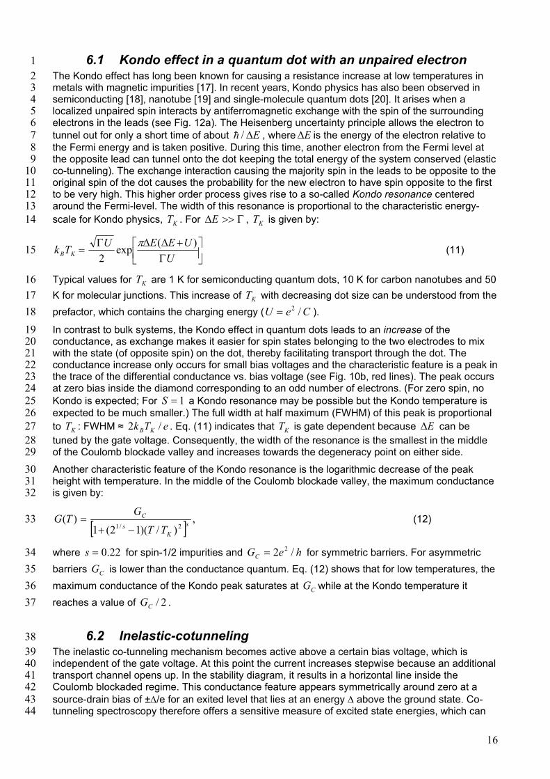
6.1 Kondo effect in a quantum dot with an unpaired electron 1 2 3 4 5 6

The Kondo effect has long been known for causing a resistance increase at low temperatures in metals with magnetic impurities [17]. In recent years, Kondo physics has also been observed in semiconducting [18], nanotube [19] and single-molecule quantum dots [20]. It arises when a localized unpaired spin interacts by antiferromagnetic exchange with the spin of the surrounding electrons in the leads (see Fig. 12a). The Heisenberg uncertainty principle allows the electron to tunnel out for only a short time of about E∆/h , where E∆ is the energy of the electron relative to the Fermi energy and is taken positive. During this time, another electron from the Fermi level at the opposite lead can tunnel onto the dot keeping the total energy of the system conserved (elastic co-tunneling). The exchange interaction causing the majority spin in the leads to be opposite to the original spin of the dot causes the probability for the new electron to have spin opposite to the first to be very high. This higher order process gives rise to a so-called Kondo resonance centered around the Fermi-level. The width of this resonance is proportional to the characteristic energy-scale for Kondo physics, T . For

7 8 9

10 11 12 13

K Γ>>∆E , is given by: KT14

Γ+∆∆Γ

=U

UEEUTk KB)(exp

2π

(11) 15

16 17 18 19 20 21 22 23 24 25 26

Typical values for T are 1 K for semiconducting quantum dots, 10 K for carbon nanotubes and 50 K for molecular junctions. This increase of T with decreasing dot size can be understood from the prefactor, which contains the charging energy (U ).

K

K

Ce /2=

In contrast to bulk systems, the Kondo effect in quantum dots leads to an increase of the conductance, as exchange makes it easier for spin states belonging to the two electrodes to mix with the state (of opposite spin) on the dot, thereby facilitating transport through the dot. The conductance increase only occurs for small bias voltages and the characteristic feature is a peak in the trace of the differential conductance vs. bias voltage (see Fig. 10b, red lines). The peak occurs at zero bias inside the diamond corresponding to an odd number of electrons. (For zero spin, no Kondo is expected; For a Kondo resonance may be possible but the Kondo temperature is expected to be much smaller.) The full width at half maximum (FWHM) of this peak is proportional to T : FWHM ≈ . Eq. (11) indicates that T is gate dependent because

1=S

e/K Tk KB2 K E∆ can be tuned by the gate voltage. Consequently, the width of the resonance is the smallest in the middle of the Coulomb blockade valley and increases towards the degeneracy point on either side.

27 28 29 30 31 32

]

Another characteristic feature of the Kondo resonance is the logarithmic decrease of the peak height with temperature. In the middle of the Coulomb blockade valley, the maximum conductance is given by:

[ ,)/)(12(1

)(2/1 s

Ks

C

TT

GTG

−+= (12) 33

34 35 36 37

38 39 40 41 42 43 44

where for spin-1/2 impurities and G for symmetric barriers. For asymmetric barriers G is lower than the conductance quantum. Eq. (12) shows that for low temperatures, the maximum conductance of the Kondo peak saturates at while at the Kondo temperature it reaches a value of .

22.0=s

C

heC /2 2=

CG2/CG

6.2 Inelastic-cotunneling The inelastic co-tunneling mechanism becomes active above a certain bias voltage, which is independent of the gate voltage. At this point the current increases stepwise because an additional transport channel opens up. In the stability diagram, it results in a horizontal line inside the Coulomb blockaded regime. This conductance feature appears symmetrically around zero at a source-drain bias of ±∆/e for an exited level that lies at an energy ∆ above the ground state. Co-tunneling spectroscopy therefore offers a sensitive measure of excited state energies, which can

16

1 2 3 4 5 6 7 8 9

be electronic or vibrational. Often in combination with Kondo peaks, inelastic cotunnelling lines are commonly observed in semiconducting, nanotube and molecular quantum dots. In Figure 13a an example of inelastic co-tunnel lines (dashed horizontal lines) for a metallic nanotube quantum dot is shown.

Figure 13b sketches the mechanism of inelastic co-tunneling. An occupied state lies below the Fermi level. It can only virtually escape from it for some small time governed by the Heisenberg uncertainty relation. If an electron from the left lead in the meantime tunnels onto the dot in the excited level (red), effectively one electron has been transported from left to right. The dot is left in an excited level and the energy difference has to be paid by the bias voltage and this two-step

process is thus only possible for exEe/EV ex> . Relaxation inside the dot may put the dot in the

ground state again. 10 11

12 13 14

Acknowledgement We thank Menno Poot for critical reading of this manuscript.

17

1 2 3

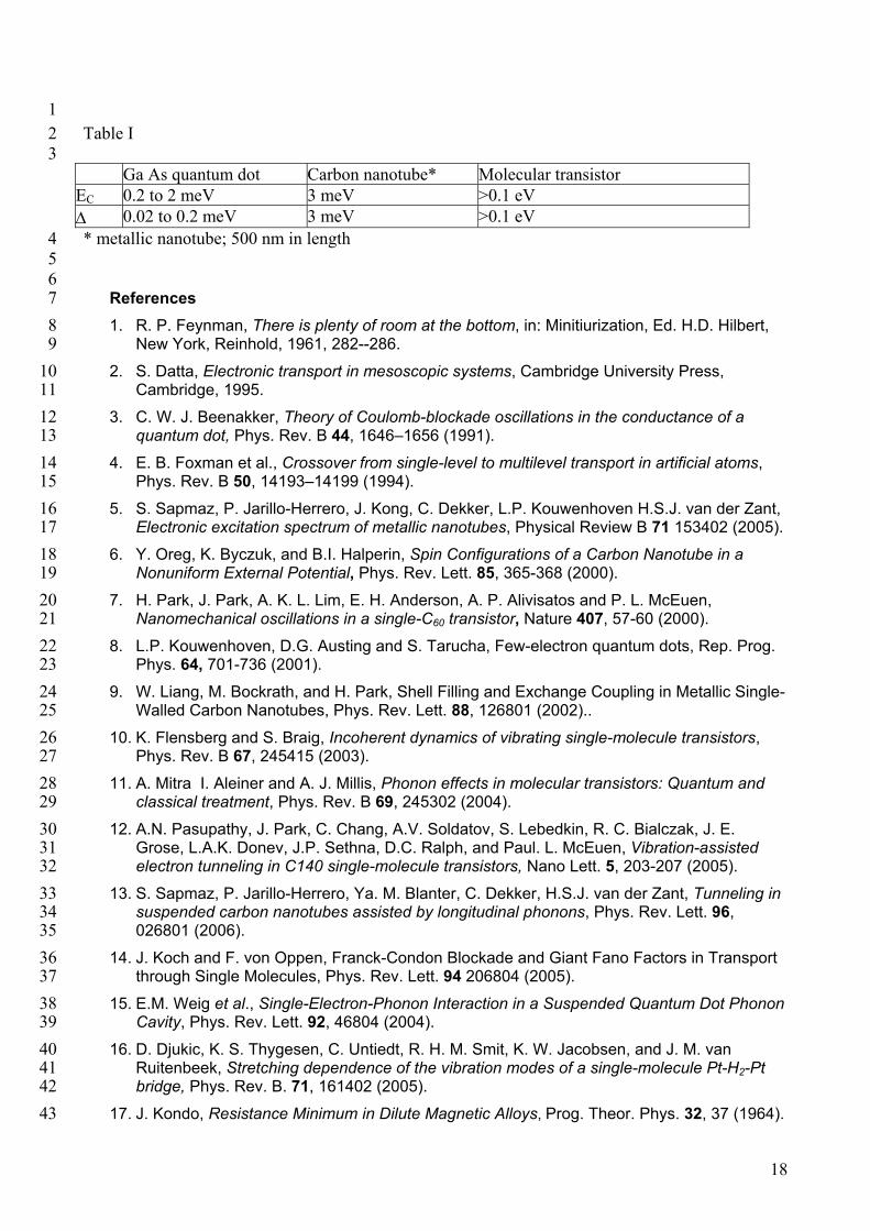
Table I

Ga As quantum dot Carbon nanotube* Molecular transistor EC 0.2 to 2 meV 3 meV >0.1 eV ∆ 0.02 to 0.2 meV 3 meV >0.1 eV

4 5 6 7 8 9

10 11 12 13 14 15 16 17 18 19 20 21 22 23 24 25 26 27 28 29 30 31 32 33 34 35 36 37 38 39 40 41 42 43

* metallic nanotube; 500 nm in length

References 1. R. P. Feynman, There is plenty of room at the bottom, in: Minitiurization, Ed. H.D. Hilbert,

New York, Reinhold, 1961, 282--286.

2. S. Datta, Electronic transport in mesoscopic systems, Cambridge University Press, Cambridge, 1995.

3. C. W. J. Beenakker, Theory of Coulomb-blockade oscillations in the conductance of a quantum dot, Phys. Rev. B 44, 1646–1656 (1991).

4. E. B. Foxman et al., Crossover from single-level to multilevel transport in artificial atoms, Phys. Rev. B 50, 14193–14199 (1994).

5. S. Sapmaz, P. Jarillo-Herrero, J. Kong, C. Dekker, L.P. Kouwenhoven H.S.J. van der Zant, Electronic excitation spectrum of metallic nanotubes, Physical Review B 71 153402 (2005).

6. Y. Oreg, K. Byczuk, and B.I. Halperin, Spin Configurations of a Carbon Nanotube in a Nonuniform External Potential, Phys. Rev. Lett. 85, 365-368 (2000).

7. H. Park, J. Park, A. K. L. Lim, E. H. Anderson, A. P. Alivisatos and P. L. McEuen, Nanomechanical oscillations in a single-C60 transistor, Nature 407, 57-60 (2000).

8. L.P. Kouwenhoven, D.G. Austing and S. Tarucha, Few-electron quantum dots, Rep. Prog. Phys. 64, 701-736 (2001).

9. W. Liang, M. Bockrath, and H. Park, Shell Filling and Exchange Coupling in Metallic Single-Walled Carbon Nanotubes, Phys. Rev. Lett. 88, 126801 (2002)..

10. K. Flensberg and S. Braig, Incoherent dynamics of vibrating single-molecule transistors, Phys. Rev. B 67, 245415 (2003).

11. A. Mitra I. Aleiner and A. J. Millis, Phonon effects in molecular transistors: Quantum and classical treatment, Phys. Rev. B 69, 245302 (2004).

12. A.N. Pasupathy, J. Park, C. Chang, A.V. Soldatov, S. Lebedkin, R. C. Bialczak, J. E. Grose, L.A.K. Donev, J.P. Sethna, D.C. Ralph, and Paul. L. McEuen, Vibration-assisted electron tunneling in C140 single-molecule transistors, Nano Lett. 5, 203-207 (2005).

13. S. Sapmaz, P. Jarillo-Herrero, Ya. M. Blanter, C. Dekker, H.S.J. van der Zant, Tunneling in suspended carbon nanotubes assisted by longitudinal phonons, Phys. Rev. Lett. 96, 026801 (2006).

14. J. Koch and F. von Oppen, Franck-Condon Blockade and Giant Fano Factors in Transport through Single Molecules, Phys. Rev. Lett. 94 206804 (2005).

15. E.M. Weig et al., Single-Electron-Phonon Interaction in a Suspended Quantum Dot Phonon Cavity, Phys. Rev. Lett. 92, 46804 (2004).

16. D. Djukic, K. S. Thygesen, C. Untiedt, R. H. M. Smit, K. W. Jacobsen, and J. M. van Ruitenbeek, Stretching dependence of the vibration modes of a single-molecule Pt-H2-Pt bridge, Phys. Rev. B. 71, 161402 (2005).

17. J. Kondo, Resistance Minimum in Dilute Magnetic Alloys, Prog. Theor. Phys. 32, 37 (1964).

18

19

1 2 3 4 5 6 7 8 9

10 11 12 13

18. D. Goldhaber-Gordon, H. Shtrikman, D. Mahalu, D. Abusch-Magder, U. Meirav, and M. A. Kastner, Kondo effect in a single-electron transistor, Nature 391, 157-159 (1998); S.M. Cronenwett, T.H. Oosterkamp and L.P. Kouwenhoven, A tunable Kondo effect in quantum dots, Science 281, 540-544 (1998).

19. J. Nygård, D.H. Cobden and P.E. Lindelof, Kondo physics in carbon nanotubes, Nature 408, 342-346 (2000).

20. J. Park et al., Coulomb blockade and the Kondo effect in single-atom transistors, Nature 417, 722-725 (2002); W. Liang, M. P. Shores, M. Bockrath, J. R. Long and H. Park, Kondo resonance in a single-molecule transistor, Nature 417, 725-729 (2002); L. H. Yu, Z. K. Keane, J. W. Ciszek, L. Cheng, J. M. Tour, T. Baruah, M. R. Pederson and D. Natelson, Kondo Resonances and Anomalous Gate Dependence in the Electrical Conductivity of Single-Molecule Transistors, Phys. Rev. Lett. 95, 256803 (2005).