Embed Size (px)
Citation preview

Louisiana State UniversityLSU Digital Commons
LSU Doctoral Dissertations Graduate School
2007
Characterization of Unsaturated Soils Using Elasticand Electromagnetic WavesBashar AlramahiLouisiana State University and Agricultural and Mechanical College, [email protected]
Follow this and additional works at: https://digitalcommons.lsu.edu/gradschool_dissertations
Part of the Civil and Environmental Engineering Commons
This Dissertation is brought to you for free and open access by the Graduate School at LSU Digital Commons. It has been accepted for inclusion inLSU Doctoral Dissertations by an authorized graduate school editor of LSU Digital Commons. For more information, please [email protected].
Recommended CitationAlramahi, Bashar, "Characterization of Unsaturated Soils Using Elastic and Electromagnetic Waves" (2007). LSU DoctoralDissertations. 2255.https://digitalcommons.lsu.edu/gradschool_dissertations/2255

CHARACTERIZATION OF UNSATURATED SOILS USING ELASTIC AND ELECTROMAGNETIC WAVES
A Dissertation
Submitted to the Graduate Faculty of the Louisiana State University and
Agricultural and Mechanical College in partial fulfillment of the
requirements for the degree of Doctor of Philosophy
in
The Department of Civil and Environmental Engineering
By Bashar Alramahi
B.S., Birzeit University, 2002 M.S., Louisiana State University, 2004
December, 2007

ii
To the memory of my father
&
To my mother and brother

iii
ACKNOWLEDGEMENTS
I would like to express my deepest thanks to my advisors Dr. Khalid Alshibli and
Dr. Dante Fratta for the valuable help and guidance they provided throughout my
graduate study at Louisiana State University. Their efforts are deeply appreciated. I
would like to extend my thanks to the members of my committee, Dr. Dean Adrian, Dr.
Radhey Sharma, Dr. Guoping Zhang and Dr. Michael Leitner. I am grateful for the help
and support they always provided.
I would have never made it this far without the great love and support from my
dear family; my mother, my brother Shadi and his wife Orouba. Their encouragement
and prayers have given me the greatest motivation to achieve the best throughout my life.
I would like to thank all my friends and fellow graduate students for the great
time we spent together. I also thank all the student workers who helped me achieve the
research tasks of this dissertation, their efforts are deeply appreciated.
I gratefully acknowledge the financial support provided by the US Army-SBIR
Program (Topic No. A012-0225). I also acknowledge the help of Mr. Steven Trautwein
and Dr. Samir Chauhan from Trautwein Soil Testing Equipment Company, our partners
in the US Army-SBIR project, and Dr. Mark Rivers from Argonne National Labs for the
help he provided in performing the CT scans.

iv
TABLE OF CONTENTS
ACKNOWLEDGEMENTS.................................................................................... iii
LIST OF TABLES................................................................................................... vii
LIST OF FIGURES................................................................................................. viii
ABSTRACT.............................................................................................................. xv
CHAPTER 1 INTRODUCTION............................................................................ 1 1.1 Background.............................................................................................. 1 1.2 Dissertation Objectives............................................................................ 2 1.3 Dissertation Layout.................................................................................. 3
CHAPTER 2 LITERATURE REVIEW................................................................ 5 2.1 Stress, Suction, and Elastic Wave Propagation in Soils.......................... 5
2.1.1 Effective Stress in Soils.................................................................. 8 2.1.2 Effective Stress in Unsaturated Soils.............................................. 9 2.1.3 Micro-Scale Force Balance in Unsaturated Soils........................... 13 2.1.4 Soil Suction..................................................................................... 16 2.1.5 Soil Water Characteristic Curves.................................................... 16 2.1.6 Soil Suction Measurement Techniques.......................................... 19
2.2 Elastic Wave Propagation in Soils........................................................... 20 2.2.1 Measurement of Wave Velocity Using Bender Elements.............. 24
2.3 Electromagnetic Wave Parameters and Time Domain Reflectometry........................................................................................... 28 2.3.1 Soils Electrical Properties............................................................... 28 2.3.2 TDR – Principle of Operation......................................................... 30 2.3.3 The Effect of Soils Electrical Conductivity on TDR
Measurements................................................................................. 34 2.3.4 TDR Probe Configurations............................................................. 37
2.4 Methods of Field Evaluation of Mass Density and Water content.......... 39 2.4.1 Traditional Field Methods............................................................... 39 2.4.2 The Purdue TDR Method................................................................ 42
CHAPTER 3 COMBINED TDR AND ELASTIC WAVE VELOCITY MEASUREMENTS TO DETERMINE IN SITU DENSITY AND MOISTURE CONTENT................................................................................................................ 45
3.1 Introduction.............................................................................................. 45 3.2 Model Derivation..................................................................................... 47 3.3 Inversion Procedure and Numerical Validation....................................... 53
3.3.1 Description of Inversion Procedure................................................ 53

v
3.3.2 Numerical Validation of the Inversion Procedure.......................... 54 3.3.3 Inversion Procedure Sensitivity Analysis....................................... 56
3.4 Experimental Setup and Soils Description.............................................. 60 3.4.1 Description of Soils.........................................................................60 3.4.2 TDR System Calibration................................................................. 61 3.4.3 Experimental Setup Description..................................................... 63 3.4.4 Specimens Descriptions.................................................................. 65
3.5 Experimental Results and Discussion...................................................... 66 3.5.1 Sources of Error.............................................................................. 68 3.5.2 Effect of Injection Hole(s) Configuration....................................... 71 3.5.3 Effect of Combined Inversion Errors.............................................. 73
3.6 Theoretical Framework for an Alternative Methodology........................ 74 3.7 Chapter Summary…................................................................................ 77
CHAPTER 4 A SUCTION-CONTROL APPARATUS FOR THE MEASUREMENT OF P AND S-WAVE VELOCITY IN SOILS...................... 79 4.1 Introduction.............................................................................................. 79
4.2 Elastic Wave Propagation in Soils........................................................... 82 4.3 Apparatus Description............................................................................. 84
4.3.1 Piezoelectric Elements.................................................................... 85 4.3.2 End Platens......................................................................................87 4.3.3 Distance between Elastic Wave Sources and Receivers................. 91 4.3.4 Saturation of the High Air Entry Disks........................................... 91
4.4 Specimen Preparation and Test Procedure.............................................. 93 4.5 Experimental Results............................................................................... 94
4.5.1 Wave Velocity Results......................................................................... 95 4.5.2 Evaluation of Results...................................................................... 99
4.6 Chapter Summary…................................................................................ 104
CHAPTER 5 THE EFFECT OF FINE PARTICLE MIGRATION ON THE SMALL STRAIN STIFFNESS OF UNSATURATED SOILS............................ 107
5.1 Introduction.............................................................................................. 107 5.1.1 Drying in Unsaturated Soils............................................................ 108
5.2 Experimental Work.................................................................................. 109 5.2.1 Apparatus Description.................................................................... 109 5.2.2 Specimens Description................................................................... 112
5.3 Experimental Results and Discussion...................................................... 115 5.3.1 Wave Velocity Results.................................................................... 115 5.3.2 Effect on Soil Stiffness................................................................... 119
5.4 Synchrotron X-ray Tomography.............................................................. 122 5.4.1 Background..................................................................................... 122 5.4.2 The Interaction of X-ray with Matter and CT Number................... 124 5.4.3 Synchrotron X-ray Facility............................................................. 124 5.4.4 Description of Tomographic Specimens......................................... 125 5.4.5 Image Analysis................................................................................126 5.4.6 Effect of Fluid on the Concentration of Fines................................ 133

vi
5.4.7 Measurement of Air-Water Interfacial Area................................... 137 5.5 Chapter Summary.................................................................................... 139
CHAPTER 6 CONCLUSIONS AND RECOMMENDATIONS......................... 142 6.1 Conclusions.............................................................................................. 142 6.2 Recommendations for Future Work.........................................................144
REFERENCES......................................................................................................... 146
VITA…..……………….………………………………………………………...... 157

vii
LIST OF TABLES
Table 2.1 Suggested effective stress equations for unsaturated soils........................ 10
Table 2.2 Evaluation of volumetric water content using TDR measurements.......... 32
Table 3.1 Synthetic values, noisy data and inverted parameters............................... 55
Table 3.2 Properties of Basic Soil Types................................................................... 60
Table 3.3 Soil Combinations Used for TDR Calibration........................................... 62
Table 3.4 Summary of tested soil specimens............................................................. 66
Table 4.1 Summary of Soil Properties...................................................................... 94
Table 5.1 Summary of Specimens’ Properties........................................................... 114

viii
LIST OF FIGURES
Figure 1.1. Shear stiffness (G) corresponding to different strain levels and the measurement methods (Atkinson and Sallfors, 1991)............................. 2
Figure 2.1. Surface through a soil mass (Mitchell, 1993).......................................... 8
Figure 2.2. The relationship between the χ parameter and the degree of saturation S. (a) χ values for a silt (after Donald, 1961); (b) χ values for compacted soils (after Blight, 1961)...................................................... 11
Figure 2.3. Surface tension of air-water interface as a function of temperature (Weast et al., 1981)................................................................................. 13
Figure 2.4. Idealized air-water interface geometry in unsaturated soil. (a) water meniscus between two spherical soil particles and (b) free-body diagram for water meniscus (Lu and Likos, 2004)................................. 14
Figure 2.5. Equivalent effective stress for simple cubic and tetrahedral packing..... 15
Figure 2.6. Total matric and osmotic suction measurements on compacted Regina Clay (Krahn and Fredlund, 1972).......................................................... 17
Figure 2.7. Representative SWCC for sand, silt and clay (Lu and Likos, 2004)....... 17
Figure 2.8 The ink bottle effect illustrated in a capillary tube model ....................... 18
Figure 2.9. Effect of the loading rate on the stress-strain behavior of unsaturated soils. (After Hoyos and Macari, 2001)................................................... 20
Figure 2.10. Types of body waves (a) P-wave (b) S-wave (Kramer 1995)............... 21
Figure 2.11. Effect of inter-particle forces on wave velocity (Fratta et al., 2001).... 22
Figure 2.12. Relationship β-exponent and θ-factor for different types of soils (after Santamarina et al. 2001).............................................................. 24
Figure 2.13. The ratio of P to S-wave velocities at different Poisson’s ratio values. 24

ix
Figure 2.14. Schematic of a piezoelectric bender element. a) series connection, b) parallel connection (Piezo systems, 2005)............................................ 25
Figure 2.15. Schematic representation of shear velocity measurement technique (Blewwett et al. 1999).......................................................................... 26
Figure 2.16. Schematic representation of the waves generated by a vibrating bender element (Lee and Santamarina, 2005)...................................... 26
Figure 2.17. Schematic of a two layer piezoelectric disk.......................................... 27
Figure 2.18. Example bender element traces............................................................. 27
Figure 2.19. Dielectric permittivity specta for solids: (a) a shale and (b) dry kaolinite (Santamarina et al., 2001)...................................................... 29
Figure 2.20. TDR System with probes vertically embedded imbedded in surface soil layer (Jones et al. 2001)................................................................. 31
Figure 2.21. Typical TDR trace and reflection points. (after Benson and Bosscher, 1999).................................................................................................... 31
Figure 2.22. Comparison of different TDR equations............................................... 33
Figure 2.23. Determination of electrical conductivity from TDR traces (Jones et al. 2001)................................................................................................ 34
Figure 2.24. The attenuation of TDR waveforms with increasing the electrical conductivity.......................................................................................... 36
Figure 2.25. TDR Probe Configurations (Jones et al., 2001).................................... 38
Figure 2.26. Schematic of the sand cone test (Multiquip, 2004)............................... 40
Figure 2.27. The water balloon apparatus.................................................................. 41
Figure 2.28. Schematic of the nuclear density test (Multiquip, 2004)....................... 42
Figure 3.1. Phase diagram: Definitions...................................................................... 48

x
Figure 3.2. Relationship between normalized skeleton shear stiffness and degree of saturation............................................................................................ 51
Figure 3.3. Modeled P-wave velocity profiles for different values of the parameter m and porosity........................................................................................ 52
Figure 3.4. Modeled Vp - θv data with (symbols) and without (lines) uniform random noise.......................................................................................... 55
Figure 3.5. Synthetic data versus inverted parameters: (a) porosity, (b) water content (c) density and (d) dry density................................................... 56
Figure 3.6. θv-Vp used for the sensitivity analysis.................................................... 57
Figure 3.7. Selected data points and inverted model response.................................. 57
Figure 3.8. 2-D projections of error matrix at: (a) constant n, (b) constant m, (c) constant Go.............................................................................................. 58
Figure 3.9. Change in error values with changing individual model parameters...... 59
Figure 3.10. Particle size distribution for the basic soil types.................................. 61
Figure 3.11. θv- κ curve developed by Soil Moisture Inc......................................... 62
Figure 3.12. TDR System Calibration....................................................................... 63
Figure 3.13. Schematic of the proposed test setup for the evaluation of in situ density and moisture content by means of combined electromagnetic and elastic wave propagation (Fratta et al. 2005)................................. 64
Figure 3.14. Application of the testing methodology to laboratory testing: (a) plastic compaction mold and TDR systems and (b) Detail of sensor and water injection hole in a compacted soil........................................ 65
Figure 3.15. Typical accelerometer traces................................................................. 65
Figure 3.16 Typical Experimental Results, fitted curve and comparison between the measured and calculated parameters............................................... 67

xi
Figure 3.17. Comparison between measured and calculated values along with error distributions (a) density (b) dry density (c) water content........... 69
Figure 3.18. Error percentage of calculated water content values for all specimens.............................................................................................. 71
Figure 3.19. (a) Single injection hole configuration, (b) multiple injection hole configuration......................................................................................... 72
Figure 3.20. Percent change in (a) density and (b) water content with ± 10% change in porosity and volumetric water content................................. 75
Figure 4.1. Poisson’s ratios corresponding to a range of P- to S-wave velocity ratios....................................................................................................... 83
Figure 4.2. Schematic of the modified triaxial apparatus, test control system and wave propagation equipment................................................................. 86
Figure 4.3. Servo-controlled air, water and cell pressure pumps............................... 87
Figure 4.4. Details of the bottom end platen: plan and cut views.............................. 89
Figure 4.5. Bottom end platen....................................................................................90
Figure 4.6. A pair of bender elements fixed in metal cups and ready to be implemented in the end platens.............................................................. 90
Figure 4.7. Minimum radius to “tip to tip” distance ratio required to ensure the first arrival of the S-wave....................................................................... 92
Figure 4.8. Grain size distribution of tested soils...................................................... 95
Figure 4.9. Wave signatures obtained for specimen 3 at increasing matric suction values. (a) P-wave traces. (b) S-wave traces. The thick lines correspond to the wave traces at stabilized matric suction values while the thin lines indicate wave traces during the stabilization process.................................................................................................... 97
Figure 4.10. Wave power spectra density calculated for specimen 3 at increasing matric suction values. (a) P-wave traces. (b) S-wave traces. The thick lines correspond to the wave power spectra at stabilized matric

xii
suction values while the thin lines indicate wave power spectra during the stabilization process............................................................. 98
Figure 4.11. Typical wave velocity response after the application of a matric suction increment (the lines just indicate trends)............................... 100
Figure 4.12. Measured P-wave velocity at increasing matric suction values........... 100
Figure 4.13. Measured S-wave velocities at increasing matric suction values.......... 101
Figure 4.14. Typical values for α and β parameters for different types of granular materials............................................................................................... 102
Figure 4.15. Modeling of wave velocities and Poisson’s ratios for soils under increasing matric suction levels............................................................ 105
Figure 4.16. Calculated S-wave velocity from shear stiffness using resonant column measurements in compacted silty sand specimens versus matric suction and net stresses data after Vinale et al. 1999): (a) compacted at optimal water content and (b) compacted wet of optimum. The data was fitted with Equation 4.12. Model parameters are shown in the figures………...... 106
Figure 5.1 Schematic plots of the different saturation stages, (a) fully saturated,(b) funicular regime, (c) pendular regime (after Mitarai and Nori, 2006)……………......................................................................... 109
Figure 5.2. Stages of unsaturated conditions and related phenomena (Cho and Santamarina, 2001)................................................................................. 110
Figure 5.3. Schematic plot of the drying cell............................................................. 111
Figure 5.4. Schematic of the drying cell end platen.................................................. 112
Figure 5.5. (a) Assembled drying cell with glass beads specimen (b) end platen with vertical and horizontal bender elements.......................................... 113
Figure 5.6. Particle size distribution of glass beads.................................................. 114
Figure 5.7. Typical wave traces obtained throughout the drying process................ 117
Figure 5.8. S- and P- wave velocities for the three drying experiments................... 118

xiii
Figure 5.9. Normalized S- and P- wave velocities for the three drying experiments............................................................................................ 118
Figure 5.10. Calculated Poisson Ratio values for the three drying experiments....... 119
Figure 5.11. Small strain shear stiffness (G) values during the drying process. (a) Calculated values, (b) Normalized values............................................ 120
Figure 5.12. Soils` constraint modulus (M) values during the drying process. (a) Calculated values, (b) Normalized values............................................ 120
Figure 5.13. Soils` bulk modulus (B) values during the drying process. (a) Calculated
values, (b) Normalized values.............................................................. 121
Figure 5.14. Schematic of the synchrotron x-ray system 13-BM-D at ANL (Culligan et al. 2004)............................................................................ 125
Figure 5.15. (a) Typical glass vial containing glass beads. (b) glass vial mounted on the CT stage..................................................................................... 126
Figure 5.16. Typical CT images (a) horizontal cross section, (b) vertical cross section................................................................................................... 127
Figure 5.17. (a) Original grayscale image (b) binary image representing the fluid phase..................................................................................................... 128
Figure 5.18. Determination of the minimum REV size............................................. 129
Figure 5.19. Histograms of CT values at different stages of drying (a) water and silt, (b) water and clay........................................................................... 130
Figure 5.20. Average overall CT numbers during drying.......................................... 131
Figure 5.21. Fluid density at different soil concentrations........................................ 131
Figure 5.22. Change in fluid density during drying process...................................... 132
Figure 5.24. Example CT image at low degree of saturation (a) gray scale, (b) enhanced contrast; blue: solid, green: water, red: air............................ 133

xiv
Figure 5.25 Example CT slice with different pore fluid bodies. Red indicated pore body fluid and yellow indicated interparticle fluid................................ 135
Figure 5.26. Average CT number for pore fluid bodies located in the pore body and interparticle contacts. (a) silt specimen (b) clay specimen............ 136
Figure 5.27 Histograms of the pore fluid and contact fluid CT numbers for clay and silt specimens.................................................................................. 137
Figure 5.29 Calculated air-water interfacial areas at different drying stages............ 140
Figure 5.30 Calculated solid-water interfacial areas at different drying stages......... 140

xv
ABSTRACT
Recent advances in laboratory instruments and techniques enabled researchers to
explore new aspects of the behavior of geomaterials and perform measurements that
would be otherwise impossible to acquire using traditional geotechnical laboratory
techniques. This dissertation is focused on utilizing elastic and electromagnetic wave
measurements and SMCT imaging to non-destructively characterize different aspects of
the behavior of unsaturated soils. A model that relates P-wave velocity in soils to the
volumetric water content was used to develop a new methodology to determine the in situ
density and moisture content of soils. It was numerically and experimentally verified to
assess it validity and range of applicability. On the other hand, a triaxial apparatus that
enables the measurement of P- and S- wave velocities in unsaturated soil specimens
under controlled net stress and matric suction was also developed. Several verification
experiments were performed using the apparatus and the results were compared to
theoretical models as well as previous experimental results. Moreover, a drying cell was
used to examine the effect of the presence of fine clay and silt particles on the elastic
waves` velocity and the small strain stiffness of unsaturated soils. The results were
confirmed by analyzing SMCT images of similar samples at different drying stages.
The proposed methodology yielded good predictions of the density and the
moisture content of soils. However, different experimental and numerical error sources
caused the predicted density and moisture content values to slightly differ from the
measured values. For the majority of the tested specimens, the density was estimated
within ±10% of the measured values while the water content was estimated within ±20%.
On the other hand, the experimental results from the new triaxial apparatus showed a

xvi
significant effect of matric suction on the recorded wave velocities. It was also
documented that wave velocity values increase with increasing percentage of fine silt
particles in the specimens.
The results of the drying cell experiments as well as the SMCT image analysis
showed the profound effect of the presence of fine silt and clay particles on the small
strain stiffness of unsaturated soils. The density of the pore fluid increased during drying
due to the higher fine concentration. The concentration of fine particles was found to be
significantly higher at areas close to the interparticle contact than in pore bodies away
from the contacts causing an increase in the interparticle contact stiffness.

1
CHAPTER 1
INTRODUCTION
1.1 Background
In common engineering applications, soils are assumed to be either dry or fully saturated.
However, in most practical cases, soils exist in a state between those two extreme states known
as unsaturated condition. The presence of both air and water in the pore space introduces a new
force balance that adds a very important component to the interparticle forces known as capillary
forces. Since the strength and deformation characteristics of unsaturated soils are controlled by
many factors including particle shapes, particle interaction, applied stresses and capillary forces,
it is very important to understand the contribution of each of these factors to the overall behavior
of geomaterials.
Recent advances in instrumentation and measurement techniques permitted better
characterization of soil properties such as stiffness at different strain levels starting from large
strains acquired by conventional laboratory testing to very small strains acquired by wave
propagation techniques. Recent research advances gave the opportunity to bridge the gap
between “low” stiffnesses typically measured using traditional laboratory tests and “high”
stiffnesses (usually denoted Gmax) measured using geophysical techniques (Wood, 2004). Figure
1.1 illustrates the levels of shear stiffness corresponding to different strain levels, and the
measurement methods used for different ranges.
Elastic wave propagation through soils is one of the most common geophysical
techniques used to determine soils small strain stiffness. The velocity of elastic waves in granular
media is determined by its stiffness; therefore, these waves provide a unique tool to monitor the
effects of different factors such as degree of saturation, suction, or applied stresses on the small

2
strain stiffness in soils and other granular materials. Moreover, because of the very small strains
associated with this type of waves, measurement could be performed without disturbing the soils
or altering any ongoing processes.
Figure 1.1 Shear stiffness (G) corresponding to different strain levels and the measurement methods (Atkinson and Sallfors, 1991)
In this dissertation, elastic waves along with electromagnetic waves and x-ray
tomography were used in various studies to determine the effects of different factors such as the
degree of saturation, matric suction and fine particle migration on the small strain stiffness of
unsaturated soils. They were also utilized to develop a new non-destructive methodology to
determine soils in situ density and moisture content.
1.2 Dissertation Objectives
This research is aimed at utilizing elastic and electromagnetic waves to characterize
different aspects of the behavior of unsaturated soils. The main objectives of the dissertation are:
1. Assess the accuracy and range of applicability of a new methodology to determine the
field density and moisture content of soils using elastic and electromagnetic waves.

3
2. Develop a new apparatus for the measurement of P- and S- wave velocities in unsaturated
soil samples under controlled net stress and matric suction.
3. Perform verification experiments using that apparatus to determine the effects of matric
suction on the P- and S- wave velocities through soils and compare the measurements to
theoretical models.
4. Determine the effects of the presence of fine silt and clay particles in the pore fluid on the
small strain stiffness of unsaturated soils during drying.
5. Monitor the changes in the properties of pore fluid containing fine silt and clay particles
at different drying stages using synchrotron x-ray computed tomography.
1.3 Dissertation Layout
This dissertation consists of six chapters. The second Chapter presents a literature review
covering the major subjects presented in the dissertation. Deferent aspects of unsaturated soils
are discussed in this chapter including effective stress expressions, soil suction, and soil water
characteristic curves. Chapter 2 describes the different types of elastic waves in soils and their
measurement techniques, and presents concepts related to electromagnetic waves propagation in
soils including the Time Domain Reflectometry (TDR) technique. Finally, Chapter 2 presents
some of the current practices for determining the in situ density and moisture content in soils.
Chapter 3 describes a new methodology for determining in situ density and moisture
content of soils using a combination of elastic and electromagnetic waves. The chapter includes a
derivation of a semi-empirical model for the P-wave velocity in soils as a function of its
volumetric water content, along with a description of the suggested methodology. It also presents
the results of numerical and experimental studies performed to assess the validity and range of
applicability of the suggested methodology.

4
The fourth Chapter is dedicated to describing a new apparatus for the measurement of P-
and S- wave velocities in unsaturated soils under controlled net stress and matric suction. It
includes a detailed description of the apparatus along with the results of experiments performed
using this apparatus. It also presents a model for the determination of S- wave velocity
considering the effects of matric suction along with a comparison between the experimentally
measured and wave velocity values based on the proposed model.
The fifth Chapter presents a study of the effects of fine particle migration on the small
strain stiffness of unsaturated soils during drying. It includes the description of a drying cell that
was developed to perform several drying experiments to determine the effects of the presence of
fine silt and clay particles in the pore fluid on the overall small strain stiffness of soils. The
results of the experiments performed using this cell along with the measured wave velocities and
the calculated stiffnesses are interpreted using synchrotron x-ray computed tomography. These
micro-tomography results show how the changes in pore fluid properties during drying increase
the fine concentration at the interparticle contacts changing the nature of the forces and
increasing the soils stiffness.
The sixth chapter presents the conclusion of the performed studies along with the
recommended future work.

5
CHAPTER 2
LITERATURE REVIEW
2.1 Stress, Suction, and Elastic Wave Propagation in Soils
2.1.1 Effective Stress in Soils
As a multi-phase particulate medium, the behavior of soils depends on the interaction of
all physical and chemical micro scale forces between the soil particles, air, and water.
Interparticle forces can be either repulsive or attractive. Repulsive forces take effect at very small
separations between particles. For example, solvation forces act at separations less than 20 Å.
They are caused by the “hard shell” effect of the molecules as the particles are getting closer. On
the other hand, electrostatic forces known as Born repulsion act at even smaller separations. It is
caused by the overlap of electron clouds between the adjacent atoms at contact points between
particles. Although these forces act at the atomic level, not the particle level, they are often
referred to as ‘interparticle reaction forces’ (Santamarina et al. 2001). Moreover, the hydration
energy of particle surfaces and inter-layer cations causes large repulsive forces at small distances
between unit layers. Hydration repulsions decay rapidly with separation distance varying
inversely as the square of the distance (Mitchell 1993).
On the other hand, when particle edges and corners are oppositely charged, electrostatic
attraction develops between them. This attraction is believed to be one of the causes of the
adherence of dry fine grained particles. At any one time there may be more electrons on one side
of the atomic nucleus than the other, creating instantaneous dipoles whose oppositely charged
ends attract each other. These are the van der Waals bonds. Electromagnetic attractions are
significant long range attractions in clays resulting from frequency dependent dipole interactions.
Although the magnitude of these forces are difficult to compute in natural soils, it is known that

6
they vary inversely as the fourth power of the separation distance between particles (Mitchell
1993).
Another source of strong long range attraction, known as Coulombian force, develops
between oppositely charged ions. The strength of this force is a function of the amplitude of the
charge of both ions and inversely related to the separation distance. However, if both ions were
similarly charged a repulsive force of similar strength will develop between them.
Cementation is a chemical bonding mechanism that can be treated as a short range
attraction where covalent and ionic bonds occur at spacing less than 3 Å. Very high contact
stresses between particles could expel adsorbed water and cations and cause mineral surfaces to
come close together providing an opportunity for cold welding. However, the absence of such
cohesion in over-consolidated silts and sands argues against such pressure induced bonding.
Since particle size is much larger than clays, interparticle contact forces should be orders of
magnitude larger as a result of fewer contacts per unit volume in coarser soils. Cementation may
also occur naturally from precipitation of calcite, silica, alumina or ion oxides or other organic or
inorganic oxides.
Another source of particle attraction is the capillary stresses in unsaturated soils. Since
water is attracted to soil particles and because water can develop surface tension, capillary
menisci form between particles in partially saturated soils. Capillary forces will be discussed
later in this section. A quantitative measure of the interaction of the mentioned forces is not
presently possible. However, a simplified expression for the inter-granular pressure can be
derived by considering the force balance through a horizontal surface through a saturated soil at
some depth (Figure 2.1). The vertical equilibrium of forces can be expressed as:
cc CauaaAAaa +=++ `σ (2.1)

7
where a is the average total cross sectional area, ac is the effective area of interparticle contacts, σ
is the applied vertical stress, u is the hydrostatic pressure, A is the long term attractive stress (i.e.,
van der Waals and electrostatic attractions), A` is the short range attractive stress (i.e., primary
valence bonding and cementation), and C is the repulsive stress resulting from hydration and
Born repulsion. Dividing all the terms in Equation 2.1 by “a” converts all the forces to stresses
per unit area of the cross section (Equation 2.2).
Auaa
AC c −+−= `)(σ (2.2)
The term aaAC c`)( − represents the intergrain force divided by the gross area, referred to
as interangular pressure (σi`). Equation 2.2 can be re-written as:
uAi −+= σσ ` (2.3)
It should be noted that u is the pore water pressure at the true interparticle zones, which is
different than the pore water pressure measured by a piezometer or other pressure measurement
devices (uo). To enable a more accurate estimate of effective stresses Bernoulli`s equation is used
to derive a relationship between u and uo as follows:
wsw hZuu γγ −−= 0 (2.4)
where Z is the elevation difference between the piezometer and the point in question, γw is the
unit weight of water, and hs is the osmotic head resulting from the difference in ionic
concentrations between points near soil particles and points away from them. Assuming no
elevation difference, and using the expression for u from Equation 2.4, Equation 2.4 can be
expressed as:
wsi huA γσσ +−+= 0` (2.5)
8
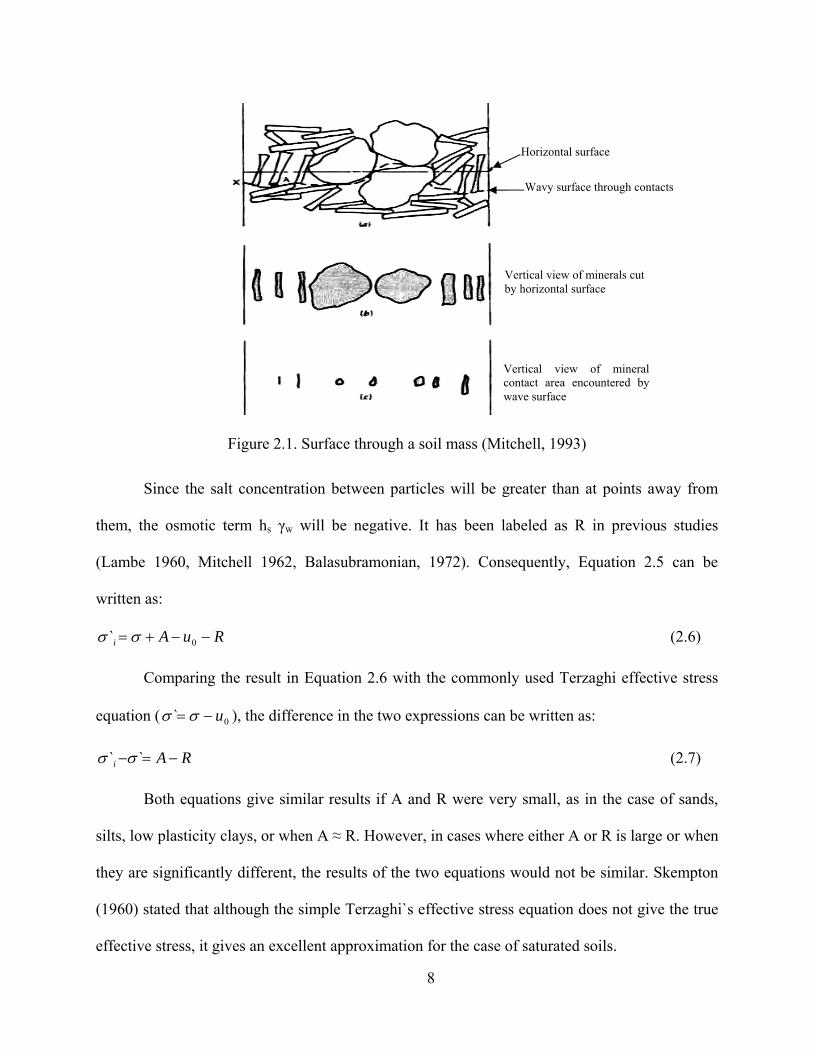
Figure 2.1. Surface through a soil mass (Mitchell, 1993)
Since the salt concentration between particles will be greater than at points away from
them, the osmotic term hs γw will be negative. It has been labeled as R in previous studies
(Lambe 1960, Mitchell 1962, Balasubramonian, 1972). Consequently, Equation 2.5 can be
written as:
RuAi −−+= 0` σσ (2.6)
Comparing the result in Equation 2.6 with the commonly used Terzaghi effective stress
equation ( 0` u−= σσ ), the difference in the two expressions can be written as:
RAi −=− `` σσ (2.7)
Both equations give similar results if A and R were very small, as in the case of sands,
silts, low plasticity clays, or when A ≈ R. However, in cases where either A or R is large or when
they are significantly different, the results of the two equations would not be similar. Skempton
(1960) stated that although the simple Terzaghi`s effective stress equation does not give the true
effective stress, it gives an excellent approximation for the case of saturated soils.
Horizontal surface
Wavy surface through contacts
Vertical view of mineral contact area encountered by wave surface
Vertical view of minerals cut by horizontal surface

9
2.1.2 Effective Stress in Unsaturated Soils
In fully saturated or fully dry soils, the Terzaghi’s effective stress principle defines the
effective stress as the difference between the total stress and the pore fluid pressure. In the case
of three phase systems (unsaturated soils) the Terzaghi’s effective stress principle is no longer
valid. The presence of air in the soil pores induces a new force balance that incorporates
capillary forces acting at the soil-air-water interface. Such forces have a direct effect on the
forces acting on particle contacts and highly influence the macroscopic behavior of the soil.
The effective stress in unsaturated soils is dependent on the relative amounts of total
stress (σ), air pressure (ua) and water pressure (uw). Many researchers proposed different forms
of effective stress relationships. Table 2.1 presents a summary of some of the equations
suggested for the effective stress in unsaturated soils.
The equation suggested by Bishop (1959) is the most general form since it includes a
term for the pressure of the gas phase. It retains the understanding that the effective stress is
made up of two components, one resulting from total normal pressure )( au−σ , and the other
from pressures exerted by the fluid in the soil pores )( wa uu − (Jennings and Burland, 1962). The
magnitude of the χ parameter is equal to unity for a saturated soil and null for a dry soil. Its
values at different degrees of saturation can be determined experimentally (e.g., Figure 2.2). It
also depends on the wetting history, loading path, soil type and internal structure of the soil
(Fredlund and Rahardjo, 1993).
The first four Equations in Table 2.1 are equivalent when the pore air pressure is the
same (β`= χ = ψ = β). Only Bishop’s form references the total and pore water pressure to the pore
air pressure. The other equations simply use gauge pressures which are referenced to the external
atmospheric pressure (Fredlund and Rahardjo, 1993). Jennings and Burland (1962) suggested

10
that under a critical degree of saturation, Bishop’s equation did not provide an adequate
description for the relationship between volume change and effective stress for most soils. The
critical degree of saturation was estimated to be approximately 20% for silts and sands and 85%
to 90% for clays. Moreover, Morgenstern (1979) stated that the Bishop’s equation proved to
“have little impact on practice. The parameter χ when determined for volume change behavior
was found to differ when determined for shear strength”.
Table 2.1. Suggested effective stress equations for unsaturated soils.
Researcher Equation Notes
Croney (1958) wu` βσσ −= Β` = a measure of the number of bonds under tension.
Bishop (1959) )()(` waa uuu −+−= χσσ Χ = a parameter related to the degree of saturation of the soil
Aitchinson (1961)
` p``σ = σ − ψ ⋅ P`` = pore water pressure difficiency. Ψ = a parameter with values ranging from zero to one
Jennings (1961) ` p``σ = σ −β⋅ P`` = negative pore water pressure taken as a positive value. β = an experimentally measured statistical factor of the same type as the contact area.
Richards (1966) )()(` assamma uhuhu −+−+−= χχσσ χm, χs = effective stress parameters for matric and solute suctions, respectively. hm, hs = matric and solute suctions, respectively.
Atchinson (1965) m m s s` p `` p ``σ = σ + χ +χ χm, χs = soil parameters ranging from 0 to 1 depending on the stress path. Pm``, ps`` = matric and solute suctions, respectively.

11
Another important limitation in Bishop’s equation is the use of soil properties in the
description of a stress state. Morgenstern (1979) stated that since the effective stress is a stress
variable, it should be related to equilibrium considerations only, however, the parameter χ bears
on constitutive behavior. Constitutive behavior is normally used in geomaterials to link
equilibrium considerations to deformations, but in this case it is introduced directly into the
stress variable. Moreover, this equation mixes global and local conditions. Both pressure and
total stress are boundary actions in Terzaghi`s effective stress equation for saturated media;
however, the pore water pressure in unsaturated soils causes a local action at the particle level
(Cho and Santamarina, 2001).
Figure 2.2. The relationship between the χ parameter and the degree of saturation S. (a) χ values for a silt (after Donald, 1961); (b) χ values for compacted soils (after Blight, 1961).
Many researchers suggested using independent stress state variables such as )( au−σ and
)( wa uu − . Numerous pairs of variables have been proposed in the literature (e.g., Coleman 1962;
Bishop and Blight 1963; and Matyas and Radhakrishna 1968). After conducting a theoretical
stress analysis, Fredlund and Morgenstern (1977) concluded that any two of three possible
normal stress variables can be used to describe the stress state of unsaturated soils. The following
three different combinations can be used as stress state variables: )( au−σ and )( wa uu − ,

12
)( wu−σ and )( wa uu − or )( au−σ and )( wu−σ . In a three dimensional stress analysis, the
stress state variables of unsaturated soil form two independent stress tensors. Using the first
couple of stress variables, the net normal stress tensor in the Cartesian coordinate system is
defined as:
σx ua−
τxy
τxz
τyx
σy ua−
τyz
τzx
τzy
σz ua−
⎛⎜⎜⎜⎝
⎞⎟⎟⎟⎠
(2.8)
and the matric suction tensor is
ua uw−
0
0
0
ua uw−
0
0
0
ua uw−
⎛⎜⎜⎜⎝
⎞⎟⎟⎟⎠
(2.9)
Under stable field conditions, the total normal stress exceeds the pore air pressure which
in turn exceeds the pore water pressure, ( wa uu >>σ ). This condition is generally true for field
conditions. However, under unique loading conditions such as blasting during mining operations,
the pore air pressure is suddenly increased to a value exceeding the total stress, resulting in a
limiting stress state condition (Fredlund and Rahardjo, 1993). Consequently, the soil skeleton
disintegrates when its tensile strength is reached.
Burland (1964) indicated that the state of stress in a soil remains constant if the values of
the net stress (σ-ua) and suction (ua-uw) are not altered. Fredlund and Morgenstern (1977)
acknowledged that suitable sets of stress state variables are those that produce no distortion or
volume change of an element when the individual components of the stress state variables are
modified but the stress state variables themselves are kept constant. They conducted a series of
“null” experiments to test different stress state variables. Similar “null” tests related to the shear

13
strength of unsaturated silt were also performed by Bishop and Donald (1961). It led to the
development of the axis translation technique that will be discussed later in Section 2.1.6.
2.1.3 Micro-Scale Force Balance in Unsaturated Soils
Surface tension (Ts) is a property of the air water interface that results from the
intermolecular forces acting on molecules in the contractile skin (Fredlund and Rahardjo 1993).
It is often defined as the maximum energy level a fluid can store without breaking apart (Lu and
Likos, 2004). It has units of energy per surface area (J/m2) or force per length (N/m). The surface
tension of pure water depends on temperature as illustrated in Figure 2.3.
Figure 2.3. Surface tension of air-water interface as a function of temperature (Weast et al., 1981)
Figure 2.4 depicts an idealized geometry of the air-water interface between two spherical
soil grains with radii r1 and r2. Considering the horizontal force balance in the horizontal
direction, three forces are considered: surface tension along the interface described by r1, surface
tension along the interface described by r2, and air and water pressure applied on either side of
the interface. The first and second forces can be expressed as (Lu and Likos, 2004):
αsin4 31 sTrF = (2.10)
αsin4 12 sTrF −= (2.11)

14
The projection of the air and water pressure ua and uw in the horizontal direction
(assuming r2 = r3) is:
αsin)(4 213 wa uurrF −= (2.12)
Figure 2.4. Idealized air-water interface geometry in unsaturated soil. (a) water meniscus between two spherical soil particles and (b) free-body diagram for water meniscus (Lu and
Likos, 2004).
Balancing the three forces leads to:
2112 )()( rruurrT was −=− (2.13)
or
⎟⎟⎠
⎞⎜⎜⎝
⎛+=−
21
11rr
Tuu swa (2.14)
Equation 2.14, known as Laplace`s equation, describes the relationship between the
matric suction (ua – uw) and the water meniscus geometry (r1 and r2). It shows that the pressure
across the air-water-solid interface depends on the relative magnitudes of r1 and r2, and could be
positive, negative, or zero. In most cases, the matric suction is positive as r1 is mostly less than r2
under unsaturated conditions (Lu and Likos, 2004).

15
Cho and Santamarina (2001) conducted a particle level study on unsaturated soils. They
considered different modes of packing and derived their effective stress equations. Two cases
were considered: simple cubic packing (coordination number 6, void ratio 0.91), and tetrahedral
packing (coordination number 12, void ratio 0.34). The effective stresses for these two cases are
shown as follows:
1 4s
eq sT 8` 2 G w
4R 9⎡ ⎤π⋅ ⎛ ⎞σ = −⎢ ⎥⎜ ⎟
⎝ ⎠⎢ ⎥⎣ ⎦ Simple cubic packing (2.15)
1 4s
eq eq,cubic sT 8` 2 2 ` 2 G w
92R
⎡ ⎤π⋅ ⎛ ⎞σ = σ = −⎢ ⎥⎜ ⎟⎝ ⎠⎢ ⎥⎣ ⎦
Tetrahedral packing (2.16)
where R is the radius of the spherical particles, Gs is the specific gravity, and w is the
water content. The authors also noted that the soil structure for uniformly graded sands at the
microscale can be constrained between the simple cubic packing and the tetrahedral packing.
Equations 2.15 and 2.16 are plotted in Figure 2.5 assuming particle radius (R) of 1 μm, specific
gravity of 2.65 and surface tension of 72.75 mN/m.
Figure 2.5. Equivalent effective stress for simple cubic and tetrahedral packing.
Gravemetric W ater Content
0.0 0.2 0.4 0.6 0.8 1.0
Equi
vale
nt E
ffec
tive
Stre
ss [k
Pa]
0
50
100
150
200
250
300
Cubic PackingTetrahedral Packing

16
2.1.4 Soil Suction
Total soil suction quantifies the thermodynamic potential of soil pore water relative to a
reference potential of free water. Free water is defined as water containing no dissolved solutes,
having no interactions with other phases that impart curvature to the air water interface, and
having no external forces other than gravity (Lu and Likos, 2004). The total suction ψ of a soil
consists of two components: osmotic suction π and the matric suction (ua – uw). Osmotic suction
is the component that results from the presence of dissolved salts in the pore water. It is present
in saturated as well as unsaturated soils. If the salt content in a soil changes, there will be a
change in its overall volume and shear strength (Fredlund and Rahardjo, 1993).
The matric suction arises from the combined effects of capillarity (ua – uw) and short term
adsorption. It is of greater importance when studying the engineering behavior of unsaturated
soils. Figure 2.6 illustrates the relative importance of changes in osmotic suction as compared to
matric suction (Fredlund and Rahardjo, 1993). One can notice that unless fine silt or clay
particles were present in the pore liquid, osmotic suction stays almost unchanged throughout the
range of water content, and the change in the total suction can be attributed solely to the change
in matric suction.
2.1.5 Soil Water Characteristic Curves
The soil water characteristic curve (SWCC) is an important relationship in unsaturated
soils. It describes the relationship between the soil suction and water content. In more specific
terms, the SWCC describes the thermodynamic potential of the soil pore water relative to that of
free water as a function of the amount of water adsorbed by the soil system (Lu and Likos,
2004). The amount of water can be expressed as gravimetric water content (w), volumetric water
content (θ) or degree of saturation (S). Typical SWCC`s for sand, silt, and clay are shown in
Figure 2.7.

17
Figure 2.6. Total matric and osmotic suction measurements on compacted Regina Clay (Krahn and Fredlund, 1972).
Figure 2.7. Representative SWCC for sand, silt and clay (Lu and Likos, 2004).
Two processes are described in the SWCC, adsorption (wetting), and desorption (drying).
The curves for the wetting and drying do not usually coincide due to hysteretic behavior that
occurs between the two processes. This behavior is attributed to the irregularity of pore shapes
(Hanks, 1992) resulting in what is known as the “ink-bottle” effect. This concept is illustrated in
Figure 2.8 that represents a capillary tube with an irregular radius (a small radius r, and a larger

18
radius R). During a wetting process (Figure 2.8a) the tube is initially empty and the height of the
capillary rise is controlled by the smaller radius (r), and stops where the larger radius is
encountered. The value of the matric suction here is: rT2 s (where Ts is the surface tension). On
the other hand, during a drying process where the tube is initially filled with water, the height of
the capillary rise might extend beyond the large radius (R), however, the matric suction at
equilibrium in this case is still rT2 s . Therefore, for the same value of matric suction, the wetting
and drying processes have different water content values, causing the hysteretic behavior.
(a) (b)
Figure 2.8. The ink bottle effect illustrated in a capillary tube model (Lu and Likos, 2004)
Due to this irregularity, losing the pore water in the drying process and filling the pores
with water in the wetting process have completely different paths causing the hysteretic
behavior. For this reason, a differentiation must be made between the wetting and drying
characteristic curves. More water is generally retained by soil during a drying process than what
is absorbed during the wetting process under the same value of suction. Knowing the SWCC of

19
an unsaturated soil helps in the assessment of many of its properties like the coefficient of
permeability, shear strength, volumetric strain and the pore size distribution (Jian and Jian-lin,
2005).
2.1.6 Soil Suction Measurements Techniques
In typical unsaturated field conditions, the air pressure (ua) is equal to the atmospheric
pressure, and the pore water pressure is generally negative. In the laboratory, it is difficult to
perform negative pore water pressure measurements without including the effect of cavitation.
For this reason some indirect techniques are utilized to measure soil suction. The most popular
laboratory technique is known as the axis translation technique developed by Hilf (1956). It is
based on the assumption that the state of stress of a soil remains constant if the values of the net
stress (σ-ua) and suction (ua-uw) are not altered (Burland 1964). In this technique, the net stress
and suction are controlled by applying a positive water pressure, and increasing the air pressure
and the total stress by the same amount to achieve the desired net stress and matric suction. The
reference or “axis” for matric suction is “translated” from the condition of atmospheric air
pressure and negative water pressure to the condition of atmospheric water pressure and positive
air pressure without changing the state of stress of the soil (Lu and Likos, 2004).
Axis translation is accomplished by separating the air and water phases of the soil
specimen. This is achieved using high air entry (HAE) porous stones in the drainage system.
When saturated, HAE materials prevent the seepage of air into the drainage system as long as the
difference between the air pressure and water pressure is less than the air entry value. Macari and
Hoyos (2001) and Hoyos and Macari (2001) developed a cubical true triaxial device where
unsaturated soils can be tested under controlled suction using the axis translation technique for a
wide range of stress paths. They conducted a series of drained true triaxial experiments on silty
sand and concluded that matric suction has a significant influence on the stress-strain behavior of

20
unsaturated soils. It was found to exert a paramount influence on the size, position, and shape of
the potential failure envelopes in the octahedral stress plane. This study also examined the
influence of the loading rate on stress-strain behavior of the specimen (Figure 2.9). They stated
that loading should be at a rate slow enough to ensure that the water menisci would not be
disturbed resulting in the loss of matric suction.
Figure 2.9. Effect of the loading rate on the stress-strain behavior of unsaturated soils. (After Hoyos and Macari, 2001)
2.2 Elastic Wave Propagation in Soils
Elastic waves can be defined as small mechanical perturbations that traverse particulate
media without causing permanent effects or altering on-going processes (Santamarina et al.
2001). The physical interpretation of the measurements of these waves permits inferring
important information about the particulate material and its processes (Choi et al. 2004). In an
infinite elastic medium, there are two types of body waves: Compressional or primary waves (P-
waves) where the particle motion and the wave propagation are in the same direction (Figure
2.10a), and shear or secondary waves (S-waves) where the particle motion is perpendicular to the
direction of wave propagation (Figure 2.10b).

21
Figure 2.10. Types of body waves (a) P-wave (b) S-wave (Kramer 1995)
The propagation of elastic waves in geophysical studies involves strain levels that are
lower than the threshold strain of the soil. The propagation velocity through a medium is
proportional to its stiffness and inversely proportional to its density. The shear wave velocity (Vs
in Equation 2.17) depends on the shear modulus of the soil (Gsoil) which is only dependent on the
skeleton shear stiffness and not influenced by the bulk stiffness of the pore fluid. For this reason,
S-waves are preferred for the characterization of saturated soils (Santamarina et al. 2005).
soil
soils
GV
ρ= (2.17)
where ρsoil is the mass density of the soil mass. Gsoil is determined by the state of stress,
degree of cementation, and by processes that alter the interparticle contacts such as capillary
forces and electrical forces. On the other hand, the propagation velocity of P- waves (Vp in
Equation 2.18) is proportional to the constraint modulus Msoil.

22
σ-increases → V-increases
log(Vs)
log(σ')
θ=Vs at σ=1kPa
Cementation increases V-increases
log(σ')
cementation log(Vs)
Sr and ρ decrease Vs increases
Vs
Sr 1 0
capillary forces increase
soil
soilsoil
soil
soilp
G34BM
Vρ
+=
ρ= (2.18)
where Bsoil is the bulk modulus of the soil. The bulk stiffness of the mineral grains Bg is
much greater than the bulk stiffness of the granular skeleton Bsk. Furthermore the bulk stiffness
of de-aired fluids Bfl (or Bw in the case of water) is also greater than the bulk stiffness of the
skeleton. However, even minute quantities of air in the fluid phase drastically reduce the bulk
modulus of fluid mixture (Richart et al. 1970). Detailed equations for the soils bulk modulus will
be presented in Section 3.2.
When the soil is fully saturated, the bulk modulus is dominated by the bulk modulus of
water which is very high, resulting in a very high propagation velocity. Hence, this kind of wave
is not preferred when studying saturated soils. Figure 2.11 shows the increase in the wave
velocity with increasing the effective stresses and cementation. It also shows the decrease in the
wave velocity with increasing the degree of saturation which is caused by the decrease in
capillary forces with the increase in the degree of saturation.
Figure 2.11. Effect of inter-particle forces on wave velocity (Fratta et al., 2001)

23
White (1983) presented a generalized relationship between P-wave velocity and effective
isotropic stress σ` in a simple cubic packing as:
612
1
s
61
22s
2s
P `6)1(8
E3V σ⋅⎥
⎦
⎤⎢⎣
⎡ρ⋅π
⋅⎥⎦
⎤⎢⎣
⎡ν−
= (2.19)
where Es, υs, ρs are the Young’s modulus, Poisson’s ratio, and mass density of the spherical
particles. For random particle arrangements, Roessler (1979) and Stokoe (1991) presented a
predictive empirical equation for the shear wave velocity in saturated or dry particulate materials
as:
β⊥
⎟⎟⎠
⎞⎜⎜⎝
⎛ σ+σθ=
r
||S p2
``V (2.20)
where θ and β depend on particle type and agreement (Figure 2.12), σ` and σ` are the stresses
in the direction parallel and perpendicular to the direction of wave propagation, and pr = 1 kPa is
the reference pressure. Santamarina et al. (2005) extended this expression to unsaturated
particulate materials as:
⎥⎦
⎤⎢⎣
⎡σ
⋅−+≈ =
v
rwa)0.1Sfor(SS `75.0
S)uu(1VV
r (2.21)
where ua and uw are the pore air and pore water pressures respectively, Sr is the degree of
saturation and σ`v is the vertical effective stress. The ratio of the P-wave velocity to the S-wave
velocity can be estimated using Poisson’s ratio ν as in Equation 2.22. Figure 2.13 illustrates the
P to S wave velocity ratios for ν range of 0 to 0.5.
1VV
1VV
5.0
2
s
P
2
s
P
−⎟⎟⎠
⎞⎜⎜⎝
⎛
−⎟⎟⎠
⎞⎜⎜⎝
⎛
=ν (2.22)

24
Figure 2.12. Relationship β-exponent and θ-factor for different types of soils (after Santamarina et al. 2001)
Poisson's Ratio υ
0.0 0.1 0.2 0.3 0.4 0.5
Vp/Vs
1
2
3
4
5
6
7
8
Figure 2.13. The ratio of P to S-wave velocities at different Poisson’s ratio values
2.2.1 Measurement of Wave Velocity Using Bender Elements
Piezoelectricity is a phenomenon resulting from lack of crystal symmetry or from the
electrically polar nature of crystals. When a mechanical load is applied to a piezo material, the
lattice distorts the dipole moment of the crystal and a voltage is generated. The voltage output
increases with crystal asymmetry. On the other hand, when a voltage is applied, the crystal
deforms (Lee and Santamarina, 2005).

25
Bender elements are composed of two layers of thin piezoelectric sheets glued to
opposite sides of a conductive metal shim (Figure 2.14). They can be used either as actuators or
sensors. Piezo motors (actuators) convert voltage and charge to force and motion. When an AC
voltage is applied to the bender element, one layer expands while the other contracts producing a
bending typically in the order of hundreds to thousands of microns and a force from tens to
hundreds of grams. Altering the current on the sides of element results in reversing the bending
action, which generates a vibration and hence a mechanical wave. On the other hand, piezo
generators (sensors) convert force and motion to voltage and charge. When a mechanical force
causes a suitable polarized 2-layer element to bend, one layer is compressed and the other is
stretched causing a charge to develop across each layer in an effort to counteract the imposed
strains (Piezo systems, 2005).
(a) (b)
Figure 2.14. Schematic of a piezoelectric bender element. a) series connection, b) parallel connection (Piezo systems, 2005).
Bender elements can be configured for either series or parallel operation. In series
configuration, the voltage is applied to all piezo layers at once, while in the parallel configuration
the supply voltage is applied to each layer individually. Series configuration develops twice the
voltage as the parallel, but provides only half the displacement for the same applied voltage.
Therefore it is recommended to use parallel bender elements as sources and series bender
elements as receivers.

26
Piezoelectric elements can be used is geotechnical testing to send and receive P and S-
waves. The type of wave generated depends on mounting configuration of the bender element.
The most common form is cantilever bender elements mounted on both ends of a triaxial or an
Oedometer cell (Figure 2.15) to generate and receive S-waves (e.g. Blewwett et al. 1999, Cho
and Santamarina 2001, Choi et al. 2004).
Figure 2.15. Schematic representation of shear velocity measurement technique (Blewwett et al. 1999)
Figure 2.16. Schematic representation of the waves generated by a vibrating bender element (Lee and Santamarina, 2005).

27
Bender elements also generate two P-wave side lobes normal to their plane (Figure 2.16).
Therefore, P-wave velocity can be measured, by placing sensors in the transverse direction of the
specimen. P-waves can also be generated using other kinds of piezoelectric materials. Two-layer
circular bending disks with constrained edges can be used (Figure 2.17). When a voltage is
applied to the disk, a drum-like movement is generated, creating a P wave. Another disk can be
used on the other side of the specimen to receive the waves.
Figure 2.17. Schematic of a two layer piezoelectric disk
The voltage supplied to the source element and the one generated by the receiver are
recorded using an oscilloscope. The time difference between the emitted and received signals can
be then evaluated. Knowing the distance between the source and the receiver, the wave velocity
can be calculated. Example source and receiver traces are depicted in Figure 2.18.
Figure 2.18. Example bender element traces
0 2 .10 4 4 .10 4 6 .10 4 8 .10 4
0
Source Reciever
Time (sec)
Vol
tage
(V)
Wave Arrival

28
2.3 Electromagnetic Wave Parameters and Time Domain Reflectometry
2.3.1 Soils Electrical Properties
Dielectric permittivity is a measure of the polarization of a dielectric material when
exposed to an external electric field (Mojid et al. 2003). It is a physical quantity that defines the
materials ability to store electric charges and determines the phase velocity of electromagnetic
radiation through the medium. The expression for the dielectric permittivity is defined as (Topp
et al. 1980):
⎟⎟⎠
⎞⎜⎜⎝
⎛⎟⎟⎠
⎞⎜⎜⎝
⎛++=
0
* '''ωεσ
κκκ dcj (2.23)
where κ* is the complex dielectric permittivity, κ’ and κ’’ are the real and imaginary parts of the
dielectric permittivity, respectively, σdc is the zero frequency conductivity, ω is the angular
frequency, εo is the free space permittivity (8.85×10⁻¹² F/m), and the imaginary term j2 is equal to
-1. Davis and Annan (1977) indicated that in the 1 MHz to 1 GHz frequency range the real part
of the dielectric permittivity does not appear to be strongly dependent on frequency. They also
indicated that the dielectric loss κ’’ was considerably less than κ’ in this frequency range (e.g.,
Figure 2.19). The propagation velocity (V) of an electromagnetic wave in a transmission line of a
known length is expressed as (Topp et al. 1980):
2tan11'
2 δκ ++=
cV (2.24)
where c is the velocity of an electromagnetic wave in free space (3 * 10-8 m/s) and tan(δ) is the
loss tangent defined as:
'
''tan 0
κωεσ
κδ
⎟⎟⎠
⎞⎜⎜⎝
⎛+
=
dc
(2.25)

29
In the case of most geotechnical applications, the loss tangent has been very small (<<1), then
Equation 2.25 can be simplified to:
'kcV = (2.26)
Figure 2.19. Dielectric permittivity specta for solids: (a) a shale and (b) dry kaolinite (Santamarina et al., 2001)
When Equation 2.26 is valid (i.e. low loss condition), κ’ is referred to as the apparent
dielectric permittivity κa. From Equation 2.26, if the apparent dielectric permittivity of the
medium is known, the velocity of the pulse can be determined, or if the velocity of the pulse is
known, the dielectric permittivity can be calculated.

30
For a multiphase system such as soils, the bulk dielectric function depends on the volume
fraction of soil solids, water, and air in the medium. The dielectric permittivity is typically 80 for
liquid water (at 20˚ C), 3 to 8 for soil minerals, and unity for air. One can notice that the amount
of water present in the soil controls the value of the bulk dielectric permittivity due to the high
value of its dielectric permittivity. Furthermore the bulk dielectric permittivity is relatively
insensitive to soil composition and texture due to the large disparity of dielectric permittivity
values (Jones et al., 2001).
2.3.2 TDR - Principle of Operation
Time Domain Reflectometry (TDR) is a non-destructive method that uses
electromagnetic pulses to measure the travel time along probes inserted in soils. Such travel time
is then used to calculate the electromagnetic wave velocity and the dielectric permittivity and to
estimate the volumetric water content which is defined as the ratio of the volume of water to the
total volume. TDR has long been used in the telecommunications industry to detect faults and
discontinuities in data transfer cables. It was first used by Topp et al. (1980) to measure soil
water content.
The TDR system sends a high frequency pulse signal to a sensor through a coaxial cable
(Figure 2.20). Reflections are recorded from any discontinuities in impedance along the path of
the signal (Mojid, 1998). The trace of the reflected pulses is recorded and the travel time is
measured. In geotechnical applications, the reflections are caused by the mismatch in the
electromagnetic impedance between the cable and the soil along the waveguide. Knowing the
time between the two reflections and the length of the probes, the travel velocity in the soil
medium can be calculated. A typical TDR trace is shown in Figure 2.21 and the reflections as the
pulse travels in the soil are illustrated.

31
Figure 2.20. TDR System with probes vertically embedded in surface soil layer (Jones et al. 2001)
Figure 2.21. Typical TDR trace and reflection points. (after Benson and Bosscher 1999)
After analyzing the TDR trace, the time required for the electromagnetic pulse to travel to
the end of the probe and the bulk dielectric permittivity is obtained using the following
relationship:
22
2⎟⎠⎞
⎜⎝⎛=⎟
⎠⎞
⎜⎝⎛=
Lct
vc
bκ (2.27)
Time

32
where t is the time required for the pulse to travel the length of the embedded probe and come
back, and L is the length of the probe. As mentioned earlier, the value of the bulk dielectric
permittivity is mainly controlled by the fraction of water in the medium. Several researchers
have developed equations relating the soil dielectric permittivity to the volumetric water content
(θv). Some common equations are listed in Table 2.2. It can be noticed that while some equations
use the dielectric permittivity as the only parameter to calculate the volumetric water content
others incorporate other parameters such as the porosity (n) and the soil bulk density ρ. Although
good correlations were obtained using only the dielectric permittivity, adding these physical
properties could yield better correlations since the volumetric water content is highly influenced
by the porosity and bulk density. Figure 2.22 shows a comparison between these correlations.
For the practical range of volumetric water content of 0 to 0.3, the values predicted by the
different equations are very close to each other.
Table 2.2. Evaluation of volumetric water content using TDR measurements Researcher Equation
Topp et al. (1980) 2 2 4 2 6
v 5.3 10 2.92 10 5.5 10 4.3 10− − − −θ = − ⋅ + ⋅ ⋅ κ − ⋅ ⋅ κ + ⋅
Wensink (1993) v 1.294 1.486 0.063θ = − + + ⋅ κ
Mixture equation (β≈0.5) ( ) s a
vw a
1 n nβ β β
β β
κ − − ⋅ κ − ⋅ κθ =
κ − κ
Malicki et al. (1996) 2
v0.819 0.168 0.159
7.17 1.18κ − − ⋅ρ − ⋅ρ
θ =+ ⋅ρ
Sources: Topp et al. (1980); Benson and Bosscher (1999); Jones et al. (2001); Noborio (2001); Santamarina et al. (2005)
The electrical conductivity of soils can also be determined using waveforms of the TDR
system. The Giese and Tiemann (1975) thin section approach gives the most accurate results for
the soil electrical conductivity (Zegelin, 1989, Benson and Bosscher, 1999, Jones et al., 2001).
The Giese-Tiemann’s equation can be written as:

33
⎟⎟⎠
⎞⎜⎜⎝
⎛−= 1
2)/( 000
fc VV
ZZ
Lc
mSECε
(2.28)
where Zo is the characteristic probe impedance and Zc is the TDR cable tester output
impedance (typically 50 Ω). V0 is the incident pulse voltage and Vf is the return pulse voltage
after multiple reflections have died out (Figure 2.23). The probe characteristic impedance is
determined using a separate calibration procedure by immersing the probe in deionized water
with known dielectric permittivity ε (Equation 2.29).
⎟⎟⎠
⎞⎜⎜⎝
⎛−
=10
10 2 VV
VZZ c ε (2.29)
Figure 2.22. Comparison of different TDR equations.
Jones et al. (2001) listed the benefits of using TDR over other soil water content
measurement methods as:
• Superior Accuracy (±2% of θv).
• Minimal calibration requirements; usually no soil-specific calibration is needed.
κ
20 40 60 80
θ v
0.0
0.2
0.4
0.6
0.8
1.0
Topp et al. (1980)Wensink (1993)Mixture equation Maliki et al. (1996)

34
• Lack of radiation hazard.
• Excellent spatial resolution.
• Measurements are simple to acquire.
Figure 2.23. Determination of electrical conductivity from TDR traces (Jones et al. 2001).
2.3.3 The Effect of Soils Electrical Conductivity on TDR Measurements
Many conflicting results have been published in the literature to describe the effect of
electrical conductivity on the estimated dielectric permittivity and volumetric water content and
volumetric water content of the medium (Nadler et al., 1999). Some researchers stated that
increasing the salinity of the soil solution can cause over-estimation of the water content (Dalton,
1992; Noborio et al., 1994; Wyseure et al., 1997). They argued that the increase in the electrical
conductivity causes an increase in the imaginary part of the dielectric permittivity causing the
apparent dielectric permittivity to be overestimated, therefore, the volumetric water content to be
over-estimated. Wyseure et al. (1997) presented Equation 2.30 to estimate the increase in the
Masked reflection due to high conductivity

35
apparent dielectric permittivity (κa) caused by the increase in the soils electrical conductivity (σ).
On the other hand, Robinson et al. (1999) presented Equation 2.31 to calculate κa.
σ+ε=κ 31.14ra (2.30)
σ+ε=κ 72.1ra (2.31)
where εr is the relative dielectric permittivity. Other researchers found no change in the estimated
water content (Topp et al., 1980; Dalton and van Genuchten, 1986; Nadler et al., 1991) whereas
some researchers found a decrease in the water content with the solution salinity (Herkelrath et
al., 1991; Nielsen et al., 1995; Vogeler et al., 1996).
Increasing the conductivity of the medium causes the attenuation of the electromagnetic
pulse as it passes through it. This situation results in the reduction of the voltage returned to the
cable tester (V2 in Figure 2.24). Dalton et al. (1984) conducted a study on ten different soil
columns with different conductivity values and compared the waveforms to determine the effect
of the soils electrical conductivity on TDR measurements. Figure 2.24 shows typical results of
their study as reported by O’Connor et al. (1999).
The attenuation of the waveform at high conductivity (salinity) values results in masking
the reflection at the end of the probes causing some difficulties in determining the travel time.
Dalton et al. (1992) also showed that 8 dSm-1 is the value above which over-estimation of
volumetric water content occurs. Wyseure et al. (1997) stated that increasing the electrical
conductivity causes the loss of energy and hinders the propagation velocity of the
electromagnetic pulse. Similar result was obtained by Hook et al. (2004). They concluded that
the travel time of the pulse increases with increasing the pore water salinity and that the
variability of travel time measurements increases, which leads to uncertainties in the measured
water content. Hook et al. (2004) suggested that it would be impossible to form a general

36
correction for the effect of salinity on the measured volumetric water content under spatially
variable field conditions even if the electrical conductivity is known. In their study, the effect of
salinity on water content error were not apparent until the salinity of the sands under test reached
25 dSm-1. The effect of electrical conductivity on the attenuation of the signal could be decreased
using shorter probes with a lower practical limit of 10 to 15 cm (Nichol et al., 2002).
Figure 2.24. The attenuation of TDR waveforms with increasing the electrical conductivity
Mojid et al. (2003) investigated the effect of the electrical conductivity on the apparent
dielectric permittivity (εa). They found that even at low values of EC the apparent dielectric
permittivity is equal to the real part of the complex dielectric permittivity (εr), which no longer
applies at high EC values. A considerable increase in the imaginary part (εi) and decrease in the
real part of the dielectric permittivity was observed for electrolyte solutions. The resulting εa was
much higher than εr. The value of εi increased sharply with decreasing the frequency of the
applied electric field.

37
2.3.4 TDR Probe Configurations
As the electromagnetic pulse is emitted, it travels through two types of transmission lines:
a coaxial cable where the electromagnetic field is constrained within the annulus between the
inner and outer conductors, and parallel rods transmission line where such constraint no longer
exists (O’Connor et al., 1999). The geometry of the rods in the TDR probe is of great importance
as it controls the degree of disturbance in the soil, the sampling volume, and the resolution of the
system. The aim of an optimal TDR probe design is to obtain a representative sampling volume
with sufficient resolution and minimal soil disturbance. Unfortunately, these factors are not
complimentary and compromises must be made to achieve the optimal design. For instance,
increasing the spacing between the rods increases the sampling volume. However, it yields in a
higher scatter of the electromagnetic field energy and a lower resolution. Moreover, increasing
the number of the rods yields a better resolution but causes more disturbance.
The length of TDR rods ranges from few centimeters to 50 cm. The practical lower limit
to maintain accuracy of the measurements is generally 10 to 15 cm (Heimovaara, 1993). Shorter
probes can be also used successfully if the volumetric water content is consistently high or with
higher frequency TDR systems (Persson and Wraith, 2002).
Many TDR probe designs have been suggested. Topp and Davis (1985) found that
parallel rod transmission lines with center to center spacing of 50 mm are a practical
compromise. They showed that the volume of the soil measured was a cylinder whose axis lies
midway between the rods with a diameter of 1.4 times the spacing between the rods. Some
designs have been proposed using two to seven rods. Another less common probe configuration
is the parallel plate probe (Robinson and Friedman, 2000) which is typically used to generate a
highly uniform electrical field between plates. Figure 2.25 shows some common TDR probe
configurations.

38
Knowing the sampling volume of the TDR probe is of great importance. Ferre et al.
(1998) defined the sampling volume as the region of porous material contributing to the TDR
measurements. Changes in the medium outside this volume have no significant impact on the
response of the instrument. Many researchers attempted to visualize the sampling volume to
determine what portion of a soil is being measured (Robinson et al., 2003; Baker and Lascano,
1989; Zegelin et al., 1989; Knight, 1992; Peterson et al.; 1995).
Figure 2.25. TDR Probe Configurations (Jones et al., 2001)
Ferre et al. (1998) compared the sampling volumes of balanced two and three rod probes.
They found that at the same spacing, an increase in the rod diameter causes a marginal
improvement in the uniformity of the distribution of the sensitivity within the sample area. The
three-rod probe had a reduced sample area and more energy around the central probe. For this
reason, Robinson et al. (2003) suggested that the two rod probes are preferable for field work.
Plates are used as an alternative to the rods in some TDR probes to produce a more
uniform energy distribution. This is done to reduce the bias of the measurements for areas close
to the rods (Robinson et al. 2003). However, using the plates causes more soil disturbance.

39
Robinson and Friedman (2000) conducted a comparison of four different probe geometries (two
and three rod probes, and two and three plate probes) and stated that at least one wetting and
drying cycle is needed for the probes to settle in the ground. Their results showed that improved
measurement precision is obtained using plates instead of rods. However, the plates might be
difficult to install and they are only suitable for non saline soils with low bulk EC due to a high
geometric factor causing rapid waveform attenuation.
2.4. Methods of Field Evaluation of Mass Density and Water Content
2.4.1. Traditional Field Methods
Many methods have been traditionally used to determine the field density and moisture
content. These methods include the sand cone and the rubber balloon. Alternative non
destructive methods have also been developed including the nuclear density gauge.
The sand cone method (ASTM D1556-00) consists of a glass or a plastic jar with a metal
cone attached to its top (Figure 2.26). The jar is filled with dry uniform Ottawa sand with known
dry density (ρsand – by laboratory calibration). After taking the combined weight of the jar, the
cone and the sand (W1), a small hole is excavated in the area where the density is to be
determined. The weight of the excavated soil is recorded (W2). Then the jar is placed on top of
the hole allowing the sand to flow out of the jar to fill the hole. The weight of the jar, the cone
and the remaining sand is then determined (W3). The weight of the sand that filled the cone and
the hole (W4) is calculated as the difference between W1 and W3. Knowing the weight of the
sand required to fill the cone (W5), the weight of the sand that filled the hole (W6) can be
calculated as the difference between W4 and W5. The volume of the hole can be calculated as:
6hole
sand
WV =ρ
(2.32)

40
Knowing the weight of the excavated soil, and the volume of the hole, the field density
can be calculated as:
2field
hole
WV
ρ = (2.33)
The rubber balloon method (ASTM D2167-94 – Figure 2.27) is similar to the sand cone
method, where a hole is excavated and the weight of the soil is recorded. The volume of the hole
is determined by inserting a rubber balloon in the excavated hole and filling the balloon with
water from a calibrated vessel. The balloon takes the shape of the hole as it is filled with water
and the volume can be directly read from the vessel.
Figure 2.26. Schematic of the sand cone test (Multiquip, 2004)
Although these two methods are widely accepted for the field density, they are time
consuming and destructive in nature. Furthermore, some inaccuracies may arise when using
these methods such as poor laboratory calibration of the density of the Ottawa sand, the volume
of the cone, and the loss of some of the soil excavated from the hole could result in the poor

41
estimation of the field density. Moreover, the cone is positioned on a perfectly flat surface during
the laboratory calibration, but this is hardly ever the case in the field. The roughness of the soil
surface in the field could result in some error in the estimated field density. Also, it should be
noted that it is not possible to ensure that the density of the Ottawa sand poured in the hole is
exactly the same as the calibration density. On the other hand, it is difficult to get the water
balloon to take the exact shape of the excavated hole, resulting in some uncertainty in the volume
reading.
Figure 2.27. The water balloon apparatus.
The nuclear density gauge (ASTM D6758-02- Figure 2.28) is a fast and fairly accurate
non destructive method to measure the field density and moisture content. Gamma rays are
emitted from a radioactive isotope source (Cesium 137) at the soil surface (backscatter) or from a
probe inserted into the soil (direct transmission - Multiquip, 2004). After passing through the
soil, a detector collects the Gamma rays and determines the soil density by examining the
absorbance of the radiation through the medium. Due to its radioactive nature, the nuclear
density gauge requires special safety procedures and certifications to transport and operate.

42
Figure 2.28. Schematic of the nuclear density test (Multiquip, 2004)
2.4.2 The Purdue TDR Method
Drnevich and his co-workers developed a methodology to determine the field density and
moisture content using TDR measurements (The Purdue Two Step Method - Siddiqui and
Drnevich 1995, Drnevich et al. 2001, Drnevich et al. 2003, ASTM D6780-02). Two
measurements are required: a field measurement and a compaction mold measurement.
Assuming a similar moisture content in the mold and in the field, the density and moisture
content in the field can be calculated. Drnevich et al. (2001) suggested using Equation 2.34 to
calculate the water content from the soils apparent dielectric constant.
⎥⎦
⎤⎢⎣
⎡−= a
bw
d
w κρρ1 (2.34)
where ρw is the density of water, ρd is the soils dry density, κ is the soils bulk dielectric
permittivity measured by TDR, a and b are calibration constants. Knowing the density of the
soil in the compaction mold, Equation 2.34 can be rewritten as:
cc
wmold
cc
w
- aw
b -
ρκ
ρ=
ρκ
ρ
(2.35)

43
where κc is the apparent dielectric permittivity in the compaction mold and ρc is the
density of the soil in the mold. Assuming the water content to be the same in the field and the
compaction mold, the field dry density can be calculated as:
f cd, f 1 w
c
κ ρρ = ⋅
+κ (2.36)
This procedure uses two soil dependent calibration constants (a and b). They are
experimentally determined for different soils through a series of compaction tests. Drnevich et al.
(2003) states that based on tests on a variety of ordinary soils the value of a is close to one and b
is approximately equal to 9.
Although this method gives quite accurate results, it still requires a field calibration
which includes excavating the soil and preparing a compaction mold and repeating the procedure
for different soils and different moisture contents in the field. Furthermore, a series of laboratory
compaction tests are required to determine the values of “a” and “b” which makes this method
time consuming and not very feasible when rapid field density and moisture content
measurements are sought.
Yu and Drnevich (2004) developed an alternative method to eliminate the need for the
compaction mold measurement, it is known as the Purdue One Step Method. It uses the electrical
conductivity that can be calculated from the TDR traces along with the bulk dielectric
permittivity to estimate the water content and dry density (Equations 2.37 and 2.38).
a bd w
d b ECa d c b
⋅ κ − ⋅ρ = ρ
⋅ − ⋅ (2.37)
a b
b a
c a ECw
b EC d⋅ κ − ⋅
=⋅ − ⋅ κ
(2.38)

44
where ECb is the bulk electrical conductivity. a, b, c and d are calibration coefficients.
This method still requires a laboratory calibration including a series of compaction tests to
determine the six coefficients for different soils.

45
CHAPTER 3
COMBINED TDR AND ELASTIC WAVE VELOCITY MEASUREMENTS
TO DETERMINE IN SITU DENSITY AND MOISTURE CONTENT
3.1 Introduction
In situ density and water content of soils are two essential properties in the design and
evaluation of many earthwork projects. They are used as criteria for acceptance and quality
control of most compaction projects including pavement systems, embankments, and clay liners.
Therefore, it is imperative to have robust, accurate, and reliable methods to ensure the proper
evaluation of these quality control parameters. Conventional and well established practices for
the evaluation of the soil density and water content include the use of simple techniques such as
the sand cone and water balloon methods which involve removing the soil for the evaluation of
water content (ASTM D1556-00; ASTM D2167-94). These methods are widely accepted;
however, they are time consuming and require the collection of specimens which makes the
process destructive. A very well known alternative is the use of the nuclear density gauge
(ASTM D3017-04) to determine both the in situ density and water content. This device allows
for the rapid determination of these parameters by monitoring the attenuation of the energy
generated by a radiation source. The radioactive nature of the device requires special
transportation, operation safety procedures, and personnel certification.
Due to limitations in the time required to collect large number of specimens and the
safety-related issues of these devices, both researchers and research & development companies
have been trying to develop new non-nuclear technologies for rapid evaluation of in situ water
content and mass density. There were many attempts toward the development of alternative
techniques with different levels of success. For example, the GeoGauge (ASTM D6758-02)

46
measures the small-strain stiffness of soils at depths one to two times the depth of its base. It can
be used as an indirect measure of the quality of compacted materials (Alshibli et al. 2005;
Sawangsuriya et al. 2003 and 2004). Other devices include the Pavement Quality Indicator (PQI)
and Soil Quality Indicator (SQI – Transtech, Inc.) which has been developed to evaluate the
quality of asphalt pavements and compacted soils (including mass density) and the Electrical
Density Gauge (Electrical Density Gauge, LLC). The SQI uses electrical impedance
spectroscopy and a calibrated artificial neural network algorithms to back-calculate the soil
density and moisture content. The Electrical Density Gauge uses a single frequency complex
impedance of soil to correlate for density and water content in bases and sub-bases. These
methods are still under performance evaluation.
A technique that is gaining acceptance and has been standardized is the Purdue TDR
method which was developed by V. Drnevich and co-workers (Siddiqui and Drnevich 1995; Lin
et al. 2000; ASTM D6780-02). It utilizes data collected using the TDR technique for soil
compacted in a mold and in situ at the same water content to estimate the in situ moisture and
dry density. The procedure involves driving four spikes into the soil surface using a template
(Drnevich et al. 2003; Yu and Drnevich 2004). Then, the multiple-rod-head-probe TDR system
is placed on the top of the spikes to measure the electromagnetic wave properties. The
measurement procedure also includes extracting a soil specimen, placing it in a compaction
mold, and measuring electromagnetic wave properties as a way to calibrate the measurements.
Based on the two sets of measurements, the water content and dry density are calculated.
Although promising results were obtained using this technique, the process of calibration and
preparing compaction molds in the field makes it time consuming and not practical when rapid
field measurements are sought. Moreover, the method uses four probes driven into the soil to

47
perform the TDR measurements that can cause disturbance to the sampled volume and alter the
density of in situ soils.
In this chapter, an alternative non-destructive, non-nuclear method for determining the in
situ density and moisture content of soils is presented. It combines the soils dielectric
permittivity data acquired using TDR with P-wave velocity measurements. A model that
correlates the P-wave velocity through soils to their volumetric water content and degree of
saturation was used to back-calculate the density and moisture content. An experimental program
was conducted to validate the proposed methodology and assess its range of applicability. The
following sub-Sections provide a detailed description of the proposed methodology, model
derivation, numerical validation and the results of the experimental program along with an
analysis of the sources of error and limitation of the proposed methodology.
3.2 Model Derivation
In this Section, a model for the P-wave travel velocity in soils is derived. Then TDR and
P-wave velocity measurements will be used to calibrate the model to find the parameters
necessary to calculate the density and moisture content of the soil. First, some basic definitions
of the soil phase relations are introduced (Figure 3.1). The soil density ρ is defined as:
arwrs )S1(nSn)n1( ρ⋅−+ρ⋅⋅+ρ⋅−=ρ (3.1)
where ρs, ρw and ρa are the density of the solids, water, and air phases; and n, Sr and θv are the
porosity, degree of saturation and volumetric water content, respectively. Knowing that the
density of air is much smaller than the density of solid and water phases, Equation 3.1 may be
reduced to:
wvswrs )n1(Sn)n1( ρ⋅θ+ρ⋅−=ρ⋅⋅+ρ⋅−=ρ (3.2)

48
Porosity (n), degree of saturation Sr (or the volumetric water content θv = nSr) and ρs (or
Gs) are needed to calculate the soil density. Gs (=ρs/ ρw) is the specific gravity of solids and
varies in a narrow range of values (from 2.6 to 2.8 for most soil minerals). The mass density of
water is assumed to be known. Then, any methodology for the evaluation of mass density and
water content should measure at least two parameters (e.g., n and Sr assuming that Gs is known
or its value is estimated).
Figure 3.1. Phase diagram: Definitions
As presented in Section 2.2, the P-wave velocity in soils is expressed as:
Soil
SoilSoil
Soil
Soilp
G34BMV
ρ
+=
ρ= (3.3)
The soil bulk modulus Bsoil is a function of the bulk modulus of the different soil
components (i.e., soil minerals, pore fluid and the stiffness of the skeleton) and their relative
quantities. Therefore, in order to quantify the overall soil stiffness, every component will be
examined separately, and then the different components will be added together to form an
expression for Bsoil. The pore fluid consists of water (with a stiffness value Bw = 2.19 × 10⁹ Pa),
and air (with a stiffness value Ba = 1.42 × 10⁵ Pa). The pore fluid stiffness can be calculated as a
function of air and water stiffnesses in addition to the degree of saturation (Sr) as:
V W
solid
water
air
Ww
Ws
Va
Vw
Vs
Vv
Volume VolumeWeight Weight
Soil Idealized soil (or phase diagram)

49
1
a
r
w
rfl B
S1BSB
−
⎟⎟⎠
⎞⎜⎜⎝
⎛ −+= (3.4)
The soil fluid suspension stiffness is defined as the stiffness of the solid particles and
fluid mixture (without the contribution of the solid particle contacts). It is a function of the
stiffness of solid mineral grains (Bg = 3.5 × 10⁹ Pa), the fluid stiffness Bfl and the porosity (n).
Bsus can be expressed as:
1
gflsus B
n1BnB
−
⎟⎟⎠
⎞⎜⎜⎝
⎛ −+= (3.5)
The stiffness of the skeleton Bsk depends on the effective stress (Roessler 1979; Stokoe
and Lee 1991; Vinale et al. 2001; Fratta and Santamarina 2002), capillary forces (Wu et al.
1984; Qian et al. 1993; Cho and Santamarina 2001), and cementation (Fernandez and
Santamarina 2001). It is related to the soil shear modulus according to the following equation:
υ−υ+
=21
132GB soilsk (3.6)
where υ is Poisson’s ratio (0.10 to 0.25 for elastic wave propagation in soils). The soil shear
modulus Gsoil depends not only on the state of stress, but also on the capillary forces (i.e., degree
of saturation) and the degree of cementation. As the proposed methodology is to be applied in
the top 15 cm of freshly compacted soils, the influence of effective vertical stresses and
cementation are insignificant with respect to the capillary forces (Cho and Santamarina 2001).
Therefore the soil shear modulus will be expressed as a function of the degree of saturation. The
challenge here is to find an equation that represents this relationship considering that two
competitive effects take that place as the degree of saturation changes. Matric suction decreases
and the cross-section of the water phase between soil particles increases as the degree of

50
saturation increases (Lu and Likos 2004). Equation 3.7 will be used to express the shear
stiffness:
m1
m1m
rorsoil 1SG)S(G ⎟⎟⎠
⎞⎜⎜⎝
⎛−⋅= − (3.7)
where m is an experimentally-determined parameter that is related to the pore size distribution of
the soil and Go is the soil shear modulus at degree of saturation Sr = 2(1-m)/m. This equation
follows a similar relationship as van Genuchten’s relationship for soil-water retention curves
(van Genuchten, 1980) as it depends on the type of soils (Wu et al., 1984; Qian et al., 1993; Cho
and Santamarina, 2001). Typical normalized shear modulus ⎟⎟⎠
⎞⎜⎜⎝
⎛
o
soil
GG
curves at different degrees
of saturation and “m” values are illustrated in Figure 3.2. The semi-empirical relationship
defined by Equation 3.7 combines both the effect of reducing suction when saturation increases
while the capillary cross sectional area increases. At 100% saturation or zero suction, the soil
shear modulus is null. Finally, the stiffness of the soil Bsoil includes the stiffnesses of the
suspension and the skeleton:
sksussoil BBB += (3.8)
Substituting Equations 3.4 to 3.8 into Equation 3.3, the P-wave velocity of a shallow
freshly compacted soil may be expressed as (Fratta et al., 2005):
rwsw
m1
m1m
ro
ga
r
w
r
p Sn)n1(G
1SG37
Bn1
BS1
BSn
1
V⋅⋅ρ+−⋅⋅ρ
⎟⎟⎠
⎞⎜⎜⎝
⎛−+
−+⎟⎟
⎠
⎞⎜⎜⎝
⎛ −+
=
−
(3.9)

51
vwsw
m1
m1m
vo
ga
v
w
v
p )n1(G
1n
G37
Bn1
Bn
B
1
Vθ⋅ρ+−⋅⋅ρ
⎟⎟⎟
⎠
⎞
⎜⎜⎜
⎝
⎛−⎟
⎠⎞
⎜⎝⎛ θ
+−
+θ−
+θ
=
−
(3.9a)
Figure 3.2. Relationship between normalized skeleton shear stiffness and degree of saturation for different m values
Equation 3.9 predicts the variation of the P-wave velocity as the skeleton shear stiffness
changes with the degree of saturation. Experimental studies have shown that such behavior
depends on the grain size distribution and texture of the grains (see for example Wu et al., 1984;
Qian et al., 1993; Cho and Santamarina, 2001). Figure 3.3 illustrates how different model
parameters, namely m and Go, can be used to fit materials that might exhibit different rate of
changes and magnitudes in the response. Note that as the volumetric water content reaches the
numerical value of the porosity, the P-wave velocity rapidly increases. This is a common
observation in both soils and weathered rocks.
0 0.2 0.4 0.6 0.80
2
4
6
8
10m = 1.5m = 2m = 4m = 8
Saturation []
Nor
mal
ized
She
ar M
odul
us []

52
Model Parameters: ρw = 9.8 kN/m3 Bw = 2.19×10⁹ Pa Ba = 1.42×10⁵ Pa Bg= 3.5×10⁹ Pa Go = 1.5×10⁶ Pa Gs = 2.7
Figure 3.3. Modeled P-wave velocity profiles for different values of the parameter m and porosity.
Parameters n, Sr (or θv), Go and m in Equation 2 should be determined by taking
consecutive measurements of the P-wave velocity in the soil while increasing its moisture
content. The following verification procedure is proposed to validate the proposed technique:
‐ Compact a soil specimen in the compaction mold
‐ Determine the weight and volume of the compacted specimen and calculate its
bulk density
‐ Determine the compacted soil gravimetric water content by oven drying method
‐ Carefully drill a water injection hole at the center of the mold, care should be
taken to minimize the disturbance of the surrounding soil
‐ Insert the TDR probes into the soil and measure the initial volumetric water
content.
‐ Determine the initial P-wave velocity using surface accelerometers

53
‐ Increase the water content in the soil by injecting water into the hole
‐ Measure the volumetric water content and the P-wave velocity
‐ Repeat the measurements with increasing water content. About four points are
required to acquire a solution for the inversion procedure
After taking multiple measurements, the parameters can be determined using a minimum
error inversion procedure that includes fitting the wave velocity model to the measured points.
The main assumption of this method is that the porosity of the soil is constant during the process.
After determining n and Sr, Equation 3.2 can be used to calculate the density of the soil. The
gravimetric water content can be calculated using Equation 3.10 (e is the void ratio):
s
r
GeS
w = (3.10)
3.3 Inversion Procedure and Numerical Validation
3.3.1 Description of the Inversion Procedure
The model described by Equation 3.9 relates the P-wave velocity to the soil volumetric
water content. The next step is to use the experimental data obtained by the proposed
methodology to calculate the parameters necessary to calculate the soils density and moisture
content. This was achieved by a minimum error inversion procedure. Such procedure considers a
range of values for n, Go and m and uses the proposed semi-empirical model to calculate the P-
wave velocity for every combination of the three variables within the defined ranges. The
calculated values are then compared to the P-wave velocity values obtained experimentally. The
error value is defined as the difference between measured and calculated P-wave velocity values:
( )∑=
><>< −=N
1i
2calculatedP
measuredP ii
VVN1Error (3.11)

54
where ><measuredPi
V is the experimentally measured P-wave velocity, ><calculatedPi
V is the P-wave
velocity calculated using the proposed model and N is the number of data points. The
combination of model variables that yields the minimum error is then selected as the solution for
the inversion problem. Some constrains are also used to assist in the convergence of the
inversion procedure; that is, the values of porosity “n” should always be equal or larger than the
highest measured volumetric water content because the volumetric water content becomes equal
to the porosity when the soil is fully saturated. Moreover, the value of parameter m should be
more than unity to ensure the inverse relationship between Vp and θv.
An algorithm was written using Matlab to perform the inversion, back-calculate the
model parameters and use them to calculate the soils density and water content. For a set of
ranges of m, Go, and n values, an array of Vp values was calculated using Equation 3.9. The error
value was then determined as the difference between the calculated and the experimentally
measured P-wave velocity values. For each combination, the determined error value was stored
in a three dimensional data array, where the x, y and z axes represent m, Go, and n values,
respectively. The algorithm then compares the error values and selects the combination of model
parameters that yield a minimum error. The inverted porosity value can then be used to calculate
density and water content.
3.3.2 Numerical Validation of the Inversion Procedure
A numerical validation was performed to assess the proper operation of the inversion
procedure. The proposed model was used to generate a synthetic data set of P-wave velocities
corresponding to assumed values of θv, n, Go and m. White random noise was added to velocity
values (±5%) and to the volumetric water content (±2%). These errors are commonly accepted in
the measurement of wave velocity and volumetric water content (Hagedoorn 1964; Noborio
2001). Table 3.1 presents the synthetic values with and without the random noise. Synthetic data

55
were then used in the inversion procedure and the calculated n, Go and m values were compared
with the original values used to generate the data. The values of the assumed and inverted
porosity and water content values are also listed in Table 3.1. Figure 3.4 illustrates the synthetic
P-wave velocity versus volumetric water content as the soil is inundated with and without the
random noise. A comparison of the assumed and inverted values of porosity, water content,
density and dry density values is illustrated in Figure 3.5.
Table 3.1. Synthetic values, noisy data and inverted parameters
# Specific gravity
Assumed Porosity
Assumed water content
Initial θv
Initial noisy θv
Initial noisy Vp
Inverted porosity
Inverted water content
1 2.6 0.35 0.10 0.169 0.166 107.0 m/s 0.346 0.094 2 2.6 0.40 0.14 0.218 0.215 128.9 m/s 0.388 0.130 3 2.7 0.37 0.12 0.204 0.204 191.4 m/s 0.374 0.121 4 2.7 0.42 0.16 0.251 0.252 144.4 m/s 0.414 0.159 5 2.8 0.40 0.14 0.235 0.231 81.3 m/s 0.398 0.142 6 2.8 0.45 0.18 0.277 0.280 145.8 m/s 0.451 0.189
Figure 3.4. Modeled Vp - θv data with (symbols) and without (lines) uniform random noise.
It can be seen from Figure 3.5 that the inversion procedure yielded close estimates of the
porosity, density, dry density and moisture content. However, due to an area of similar error
Specimen 4 Specimen 5 Specimen 6
0.1 0.15 0.2 0.25 0.3 0.3550
100
150
200
250
P-w
ave
velo
city
[m/s
]
Volumetric water content 0.1 0.15 0.2 0.25 0.3 0.3550
100
150
200
250
P-w
ave
velo
city
[m/s
]
Volumetric water content
Specimen 1 Specimen 2 Specimen 3

56
values in the inversion error matrix, some difference between the modeled and the inverted
values are noticed. This issue is discussed in detail in the following Section.
Figure 3.5. Synthetic data versus inverted parameters: (a) porosity, (b) water content (c) density and (d) dry density.
3.3.3 Inversion Procedure Sensitivity Analysis
As mentioned earlier, soils’ density and water content are calculated from the collected
volumetric water content and P-wave velocity data by means of a minimum error inversion
procedure. The inversion algorithm determines the combination of n, m, and Go values that yield
the minimum difference between the measured and calculated P-wave velocity values. In order
to investigate the effects of model parameters on the solution convergence, a sensitivity analysis
of the suggested model and inversion procedure is performed.
0 0.1 0.20
0.1
0.2
0.2 0.3 0.40.2
0.3
0.4
“Modeled” moisture content
Inve
rted
moi
stur
e co
nten
t
“Modeled” porosity
Inve
rted
poro
sity
1600 1800 2000
1600
1800
2000
1600 1800 2000
1600
1800
2000
“Modeled” soil density [kg/m3]
Inve
rted
soil
dens
ity [k
g/m
3 ]
“Modeled” dry soil density [kg/m3]
Inve
rted
dry
soil
dens
ity [k
g/m
3 ]

57
In this analysis, a set of assumed parameters was used to generate a θv-Vp curve using the
proposed model (Figure 3.6). Then, the inversion procedure was conducted on data points
selected along the generated curve, and the inverted model parameters were obtained using the
inversion procedure. Figure 3.7 illustrates the selected data points and the fitted curve obtained
from the inversion procedure. The results were used to perform a detailed analysis of the
inversion procedure and to examine the behavior of the inversion error values.
Figure 3.6. θv-Vp curve used for the sensitivity analysis
Figure 3.7. Selected data points and inverted model response
Inverted Parameters: m = 1.1 Go = 974000 Pa n = 0.351
Assumed Parameters: m = 1.1 Go = 1000000 Pa n = 0.35

58
During the inversion process, a 3D data matrix was generated to store the error values
generated for every combination of the three model parameters. To facilitate the visualization of
the error surfaces, three 2D planes representing the error values for the combination of two
model parameters while the third was held constant are displayed. Figure 3.8 illustrates the x,y
and z sections corresponding to constant values of n, m, and Go values, respectively.
Figure 3.8. 2-D projections of error matrix at: (a) constant n, (b) constant m, (c) constant Go
It can be seen from the error values in Figure 3.8 that while a minimum error value can
be clearly identified in the cases of constant n and constant Go, it is difficult to identify such
value for the case of constant m. In this case, a band of similar error values can be identified
along a wide range of n and Go values. In other words, different combinations of n and Go could
yield similar error values making it difficult to identify a unique minimum error solution (i.e.,

59
non-unique solutions are obtained). While in most cases a single minimum error solution can be
still obtained using this method, the presence of similar error values can introduce uncertainty in
the obtained solution.
To further investigate how the error values are affected by the different model
parameters, further analyses were performed where after the model parameters were obtained,
each parameter was studied separately. Therefore, two parameters were held constant while the
third was changed to determine how prominent the effect of that parameter is on the calculated
error value. Figure 3.9 illustrates the effect of changing different model parameters on calculated
error values. The higher change in the error values makes is easier to identify the minimum error
point.
Figure 3.9. Change in error values with changing individual model parameters
Figure 3.9 demonstrates that the value of parameter m has the most profound effect on
the error values, where a slight change in m will cause a sharp change in the calculated error
values. This helps in the convergence of this parameter in the inversion procedure where it is
relatively easy to recognize the value of parameter m that yields the minimum error. The value of
parameter n has a smaller effect on the obtained error where smaller error values were obtained
for the range of change of ±5%. On the other hand, it can be seen that the value of Go has the

60
smallest effect on the obtained error values. Such small change in the calculated error value
could cause some difficulty in obtaining the correct Go value because of its close similarity to the
error values obtained at neighboring Go values.
3.4 Experimental Setup and Soils Description
In order to verify the validity and range of applicability of the proposed procedure, an
experimental program was implemented where the procedure was applied to a variety of soil
types consisting of different mixtures of sand, silt and clay. The following sub-Sections include a
description of the soils used in the experiments, calibration of the TDR system and the results of
the different verification experiments.
3.4.1 Description of Soils
Four basic types of soils where used in the experimental program: Kaolinite clay (C), fine
construction sand (S), silt (M1) and silty sand (M2). Figure 3.10 depicts the grain size
distribution curves for the four soil types. The properties and USCS classification of the four soil
types are summarized in Table 3.2. These different types of soils were selected due to the range
in grain size, plasticity, and electrical conductivity. Grain size distribution controls the capillary
forces exerted in the particles (Cho and Santamarina, 2001), plasticity indicates water absorption
and swelling potential (Mitchell, 1993), and electrical conductivity controls the range of
application of the TDR methodology to evaluate volumetric water content in soils (Robinson et
al., 2003).
Table 3.2. Properties of Basic Soil Types Soil
Label Specific
Gravity (Gs) Liquid Limit
Plasticity Index
USCS Classification
D50 (mm)
Cc Cu
C 2.59 43.6 18.2 CL 0.0012 N/A N/A M1 2.64 35.5 9.0 ML 0.015 6.64 21.25M2 2.68 17.5 2.7 SM 0.21 0.66 440 S 2.65 N/A N/A SP 0.31 1.22 1.83

61
Figure 3.10. Particle size distribution for the basic soil types.
3.4.2 TDR System Calibration
The TDR system used in this study was model 6050X3K1-MiniTrase Kit manufactured
by Soilmoisture Equipment Corp. It used a two probe configuration. The probes were 150 mm
long and 50 mm apart. The system used a manufacturer-developed curve to estimate the
volumetric water content values (θv) from the measured dielectric permittivity value (κ – Figure
3.11). In order to verify the proper performance of the TDR system, a series of experiments were
performed to compare the volumetric water content values obtained by the TDR system with the
values obtained by weight and volume measurements. This was achieved by compacting
different soils in a cylindrical mold, recording their weight and volume to calculate the density
and obtaining the gravimetric water content according to oven drying procedure. These
measurements were used to calculate the soils volumetric water content. TDR readings were
taken in the mold and the obtained θv values were compared with calculated values. Table 3.3
presents the different soil mixtures used in the calibration procedure.

62
Figure 3.11. θv- κ curve developed by Soil Moisture Inc.
Table 3.3. Soil Combinations Used for TDR Calibration
Percent of Soil
Specimen Name C S M1 M2 C 100 0 0 0 S 0 100 0 0
M1 0 0 100 0 M2 0 0 0 100
C-M1 67 0 33 0 C-S 67 33 0 0
C-S-M1 33.3 33.3 33.3 0 M1-C 33 0 67 0 M1-S 0 33 67 0 S-C 33 67 0 0
S-M1 0 67 33 0 C-S-M2 33.3 33.3 0 33.3 M2-S-C 25 25 0 50
M2-S 0 50 0 50
The results of the TDR system calibration are displayed in Figure 3.12. It can be seen
that the volumetric water content values obtained by TDR measurements over-estimate θv by
about 14%. Therefore, a correction factor of 0.88 was applied to the readings of the TDR system

63
in order to obtain more accurate θv values. The difference between the calculated and measured
θv values could arise from the difference of soil types used in the development of the
manufacturer curve and the ones used in the laboratory calibration.
3.4.3 Experimental Setup Description
An experimental setup was developed to implement the proposed procedure (Figures 3.13
and 3.14). It consisted of a TDR system to measure the volumetric water content of the soil
specimens, two piezoelectric accelerometers (model: PCB 353B16) to measure the P- wave
velocity, and a digital oscilloscope (model: Fluke 192 Scopemeter) to record the wave arrival
data from the accelerometers. A special compaction mold made of plastic was used in this
procedure since using a metal mold could result in the interference of the propagation of the
electromagnetic waves through the compacted soils. The mold has a diameter of 150 mm and a
height of 200 mm.
Figure 3.12. TDR System Calibration

64
A water injection hole was drilled at the center of the mold after the soil was compacted.
Accelerometers and TDR rods were embedded into the soil. In some stiff soils, a special guide
template was used to insure that the TDR rods remain straight while being driven into the soil.
The volumetric water content was measured using the TDR system. Then, a P-wave was
generated by dropping a metal ball along the axis of the accelerometers. Knowing the distance
between the accelerometers, the wave velocity was determined by measuring the time difference
between the arrivals. Figure 3.14 shows typical accelerometer traces. After recording the
volumetric water content and the wave arrival data, the water content of the soil was increased
by adding water to the injection hole. After the water was allowed to dissipate into the soil,
another wave velocity and volumetric water content measurements were made. This procedure
was repeated until enough data points were generated to apply the inversion procedure. After the
inverted parameters were obtained, the density and moisture content were calculated and
compared to the values measured by weight-volume relationships.
Figure 3.13. Schematic of the proposed test setup for the evaluation of in situ density and moisture content by means of combined electromagnetic and elastic wave propagation (Fratta et
al. 2005).

65
Figure 3.14. Application of the testing methodology to laboratory testing: (a) Plastic compaction mold and TDR systems and (b) Detail of sensor and water injection hole in a compacted soil.
Figure 3.15. Typical accelerometer traces
3.4.4 Specimens Description
To verify the accuracy and range of applicability of the proposed methodology and
inversion procedure, a testing program was developed that includes testing different mixtures of
the four basic soil types described in Section 3.4.1. To prepare the soil specimens, the soil mix
components were thoroughly mixed to obtain a homogeneous soil mixture. Then, water was
-10
-5
0
5
10
-0.001 0.000 0.001 0.002 0.003Time [sec]
Am
plitu
de [V
]
Δt

66
added to achieve the desired initial water content. Table 3.4 summarizes properties of the tested
specimens. Soils were compacted in three layers. They were compacted in the mold at three
compaction energy levels and different initial water content values. The different compaction
efforts were achieved by varying the number of blows used to compact the soil layers. The
energies used were: 239, 398 and 592 kJ/m3, which correspond to 15, 25 and 37 blows/layer,
respectively, using the standard Proctor compaction hammer.
Table 3.4. Summary of tested soil specimens.
Percent of Soil Specimen Name C S M1 M2 Blows per layer Number of experiments
C-S-M1-15 33.3 33.3 33.3 0 15 6 C-S-M1-25 33.3 33.3 33.3 0 25 4 C-S-M1-37 33.3 33.3 33.3 0 37 8 M1-C-S-15 25 25 50 0 15 4 M1-C-S-25 25 25 50 0 25 5 M1-C-S-37 25 25 50 0 37 5
M1-S-15 0 50 50 0 15 5 M1-S-25 0 50 50 0 25 5 M1-S-37 0 50 50 0 37 5 M1-15 0 0 100 0 15 4 M1-25 0 0 100 0 25 5 M1-37 0 0 100 0 37 5
C-M2-15 33 0 0 67 15 5 C-M2-25 33 0 0 67 25 8 C-M2-37 33 0 0 67 37 2
M2-15 0 0 0 100 15 3 M2-15 0 0 0 100 15 4 M2-15 0 0 0 100 15 5
88
3.5 Experimental Results and Discussion
The proposed methodology to determine the density and moisture content was performed
on all the soil specimens listed in Table 3.4. The inversion algorithm was then used to estimate
the three model parameters: n, m and Go. Bulk density, dry density and moisture content were

67
Experiment: M1-S-15 (2) Parameter Measured Inverted
n 0.291 0.275 ρ (kg/m3) 2067 2163
w (%) 10.17 10.70 ρd (kg/m3) 1876 1954
m - 1.108 Go (Pa) - 3030000
then calculated and compared to values obtained by weight and volume measurements. This
Section presents typical experimental data along with their inversion results. A summary of the
results of all experiments and a comparison of all the measured and calculated parameters are
also presented.
After each experiment was performed, the traces from the accelerometers were analyzed
to obtain the P-wave velocity at the different θv values for all experiments. These values were
plotted to ensure that the proper trend was obtained. The experimental data was then input into
the MATLAB inversion program in order to calculate the model parameters. A wide range of the
three model parameters was initially set in the inversion program in order to find the
approximate region where the minimum error solution was located. The ranges of the three
model parameters were narrowed down in the second run in order to “fine tune” the solution. A
narrower range of values results in a smaller step size yielding an improved data resolution.
Figure 3.16 illustrates typical experimental Vp- θv data along with the curve obtained by the
inversion procedure. It also lists the measured and calculated model parameters.
Figure 3.16 Typical Experimental Results, fitted curve and comparison between the measured and calculated parameters.
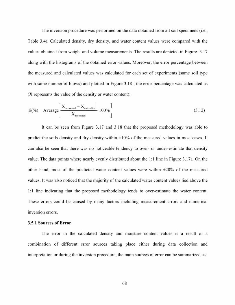
68
The inversion procedure was performed on the data obtained from all soil specimens (i.e.,
Table 3.4). Calculated density, dry density, and water content values were compared with the
values obtained from weight and volume measurements. The results are depicted in Figure 3.17
along with the histograms of the obtained error values. Moreover, the error percentage between
the measured and calculated values was calculated for each set of experiments (same soil type
with same number of blows) and plotted in Figure 3.18 , the error percentage was calculated as
(X represents the value of the density or water content):
⎥⎥⎦
⎤
⎢⎢⎣
⎡⋅
−= %100
XXX
Average(%)Emeasured
calcualtedmeasured (3.12)
It can be seen from Figure 3.17 and 3.18 that the proposed methodology was able to
predict the soils density and dry density within ±10% of the measured values in most cases. It
can also be seen that there was no noticeable tendency to over- or under-estimate that density
value. The data points where nearly evenly distributed about the 1:1 line in Figure 3.17a. On the
other hand, most of the predicted water content values were within ±20% of the measured
values. It was also noticed that the majority of the calculated water content values lied above the
1:1 line indicating that the proposed methodology tends to over-estimate the water content.
These errors could be caused by many factors including measurement errors and numerical
inversion errors.
3.5.1 Sources of Error
The error in the calculated density and moisture content values is a result of a
combination of different error sources taking place either during data collection and
interpretation or during the inversion procedure, the main sources of error can be summarized as:

69
Figure 3.17. Comparison between measured and calculated values along with error distributions (a) density (b) dry density (c) water content
(a)
(c)
(b)
-40 -30 -20 -10 0 10 20 30 400
5
10
15
Error (%)
Cou
nt
-40 -30 -20 -10 0 10 20 30 400
5
10
15
Error (%)
Cou
nt
-40 -30 -20 -10 0 10 20 30 400
5
10
15
Error (%)
Cou
nt

70
‐ P-wave velocity and volumetric water content estimation: such errors can arise during the
evaluation of the travel times of P waves and electromagnetic waves resulting in errors up
to about 10%.
‐ Non-homogeneous distribution of injected water: the value of the volumetric water
content obtained by the TDR system represent the average water content value along the
TDR sampling volume, however, during the water injection process, the distribution of
water along this volume might not be homogenous resulting in a measurement error.
Moreover, non-homogeneity causes the sampling area of the TDR to be different from
the sampling area of the P-wave velocity. The output from the TDR system represents the
average values along the depth of 150 mm whereas P-wave velocity is measured near the
surface.
‐ Local saturation of the region around the injection hole: increasing the soils water
content yields a reduction in P-wave velocity, however when the soil is fully saturated,
the P-wave velocity travels in water at a much higher velocity (~1500 m/s). Therefore,
having a locally saturated zone (even a few millimeters in size) around water injection
hole could results in errors in the measured P-wave velocity.
‐ Inversion procedure errors: as shown earlier, it is relatively easy to identify the minimum
error point in the Go–m and n–m planes. However, in the n–Go planes, a band of similar
error values was noticed. The presence of this “similar error zone” makes it difficult to
identify the inversion solution because of the close similarity to the calculated error
values for the points around it along that band.
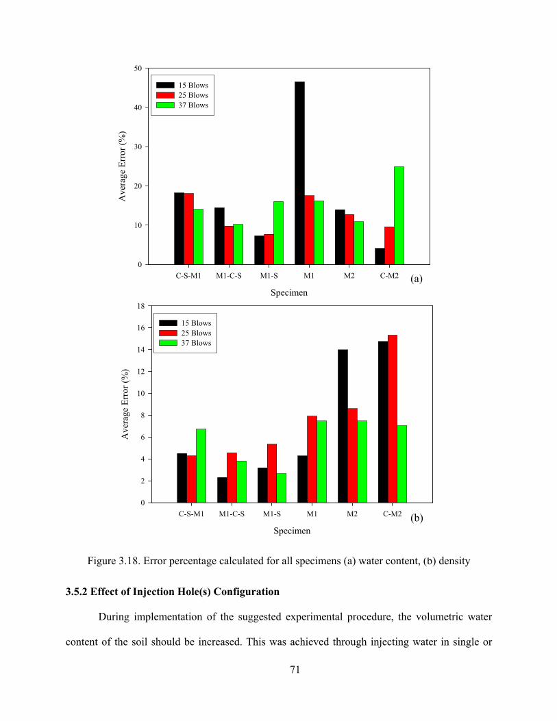
71
Figure 3.18. Error percentage calculated for all specimens (a) water content, (b) density
3.5.2 Effect of Injection Hole(s) Configuration
During implementation of the suggested experimental procedure, the volumetric water
content of the soil should be increased. This was achieved through injecting water in single or
Specimen
C-S-M1 M1-C-S M1-S M1 M2 C-M2
Ave
rage
Err
or (%
)
0
10
20
30
40
50
15 Blows25 Blows37 Blows
Specimen
C-S-M1 M1-C-S M1-S M1 M2 C-M2
Ave
rage
Err
or (%
)
0
2
4
6
8
10
12
14
16
18
15 Blows25 Blows37 Blows
(b)
(a)

72
multiple injection holes carefully drilled in the sampled volume. Initially, a single injection hole
was used to achieve this purpose (Figure 3.19a). This configuration was chosen to be able to
raise the volumetric water content without causing much disturbance to the surrounding soils.
However, due to the long time required for the water to dissipate into the soil, and in an attempt
to achieve a more homogeneous water distribution, two sets of experiments were carried out
using a multiple injection hole configuration: M2 and C-M2. This configuration consisted of five
smaller injection holes distributed around the sampled volume (Figure 3.19b).
Figure 3.19. (a) Single injection hole configuration, (b) multiple injection hole configuration
By examining the results of the inversion procedure, it can be seen that while no
significant improvement was achieved in the water content measurements, the density error
values for the two sets of experiments with the multiple hole configuration were noticeably
higher than the ones with the single hole configuration. This is believed to be caused by the
higher soil disturbance caused by drilling the five injection holes instead of one. Therefore,
although more time is required for the water to dissipate into the soil, the single injection hole
configuration seems to yield better results than the multiple hole configuration.
(b) (a)

73
3.5.3 Effect of Combined Inversion Errors
As mentioned earlier, several factors could affect the quality of the measured and
calculated parameters necessary to calculate the density and water content. Therefore, it is
important to examine the effect of such errors on these parameters. Equations 3.13 through 3.15
indicate that the main parameters affecting the values of the density and moisture content are
porosity (n) and volumetric water content (θv). Therefore, a sensitivity study was performed to
assess the effect of measurement errors of these two parameters on the calculated density and
water content values.
wvs)n1( ρθ+ρ−=ρ (3.13)
1wd
−ρρ
= (3.14)
sd )n1( ρ−=ρ (3.15)
To perform the sensitivity analysis, initial values for “n” and “ vθ ” were assumed and
used to calculate the initial density and moisture content: oρ and wo. Then, an error of ±10% was
added to the porosity and volumetric water content, and the values of density and moisture
content were calculated for the different combinations of the parameters ranging from -10% to
+10%. The resulting error in the calculated density and moisture content for each combination
was calculated using Equation 3.16. The resulting error plots are illustrated in Figure 3.20.
Density: %100),n(
(%)Eo
ojij,i ⋅
ρ
ρ−θρ= (3.16a)
Water Content: %100w
w),n(w(%)E
o
ojij,i ⋅
−θ= (3.16b)
Figure 3.20 shows that the full spectrum of porosity and volumetric water content error
values yield an error of about ±6% in the calculated density values. On the other hand, the same

74
range of error values yields and error of ±15% in the calculated water content values. This
indicates that the error in the calculated water content is more sensitive to errors in the porosity
and volumetric water content. This also justifies the higher error values obtained during the
inversion of the experimental data.
3.6. Theoretical Framework for an Alternative Methodology
As seen from the previous experimental study and error analysis, although the proposed
methodology yielded close estimates of the density and moisture content, similar error values in
the inversion algorithm caused uncertainty in the obtained solutions. Therefore, to further
improve the current methodology, other physically meaningful parameters should be added to
introduce more constraints to the inversion procedure. In this section, the feasibility of adding the
shear wave velocity Vs to the obtained measurements is investigated. A new model will be
derived assuming that Vs is measured along with Vp and vθ .
Soils bulk modulus Bsoil is calculated as the sum of the bulk modulii of the soils skeleton
Bsk and the suspension Bsus. The definitions of these parameters are presented in Section 3.2. Bsk
can be expressed as a function of the shear modulus and Poisson`s ratio (Equation 3.17). On the
other hand, substituting the values of Bfl from Equation 3.4 into Equation 3.5 yields the
expression for Bsus in Equation 3.18. Bsoil can then be calculated by adding Bsk and Bsus (Equation
3.19).
⎟⎠⎞
⎜⎝⎛
ν−ν+
⋅=21
1G32B soilsk (3.17)
1
g1
a
r
w
r
sus Bn1
BS1
BS
nB
−
−
⎟⎟⎟⎟⎟
⎠
⎞
⎜⎜⎜⎜⎜
⎝
⎛
−+
⎟⎟⎠
⎞⎜⎜⎝
⎛ −+
= (3.18)

75
Figure 3.20. Percent change in (a) density and (b) water content with ± 10% change in porosity and volumetric water content
⎟⎠⎞
⎜⎝⎛
ν−ν+
⋅+
⎟⎟⎟⎟⎟
⎠
⎞
⎜⎜⎜⎜⎜
⎝
⎛
−+
⎟⎟⎠
⎞⎜⎜⎝
⎛ −+
=
−
211G
32
Bn1
BS1
BS
nB soil
1
g
a
r
w
rsoil (3.19)
The shear stiffness Gsoil can be calculated from the density (ρ) and Vs using Equation 2.17
Substituting the values of Gsoil and ρ from Equations 2.17 and 3.2 into Equation 3.19 yields
Equation 3.20. Moreover, the P-wave velocity (Equation 3.3) is dependent on Bsoil, Gsoil, and ρ.
Porosity Error (%)
Vol
umet
ric W
ater
Con
tent
Err
or (%
)
-10 -5 0 5 10
-5
0
5
10
-6
-4
-2
0
2
4
6
Porosity Error (%)
Vol
umet
ric W
ater
Con
tent
Err
or (%
)
-10 -5 0 5 10
-5
0
5
10
-10
-5
0
5
10
15
(b)
(a)

76
Substituting the values these parameters from Equations 3.20, 2.17 and 3.2 , respectively, into
Equation 3.3 yields a new P-wave velocity model (Equation 3.21).
( ) ⎟⎠⎞
⎜⎝⎛
ν−ν+
⋅⋅ρ⋅θ+ρ⋅−+
⎟⎟⎟⎟⎟
⎠
⎞
⎜⎜⎜⎜⎜
⎝
⎛
−+
⎟⎟⎠
⎞⎜⎜⎝
⎛ −+
=21
1V)n1(32
Bn1
BS1
BS
nB 2Swvs
g
a
r
w
rsoil (3.20)
( ) [ ]
wvs
2Swvs
2Swvs
g
a
r
w
r
p )n1(
V)n1(34
211V)n1(
32
Bn1
BS1
BS
n
Vρ⋅θ+ρ⋅−
⋅ρ⋅θ+ρ⋅−+⎟⎠⎞
⎜⎝⎛
ν−ν+
⋅⋅ρ⋅θ+ρ⋅−+
⎟⎟⎟⎟⎟
⎠
⎞
⎜⎜⎜⎜⎜
⎝
⎛
−+
⎟⎟⎠
⎞⎜⎜⎝
⎛ −+
= (3.21a)
( ) [ ]
wvs
2Swvs
2Swvs
g
a
v
w
v
p )n1(
V)n1(34
211V)n1(
32
Bn1
Bn
1
Bn
n
Vρ⋅θ+ρ⋅−
⋅ρ⋅θ+ρ⋅−+⎟⎠⎞
⎜⎝⎛
ν−ν+
⋅⋅ρ⋅θ+ρ⋅−+
⎟⎟⎟⎟⎟⎟⎟⎟⎟⎟⎟
⎠
⎞
⎜⎜⎜⎜⎜⎜⎜⎜⎜⎜⎜
⎝
⎛
−+
⎟⎟⎟⎟⎟
⎠
⎞
⎜⎜⎜⎜⎜
⎝
⎛⎟⎠
⎞⎜⎝
⎛ θ−
+⎟⎠
⎞⎜⎝
⎛ θ
= (3.21b)
It can be seen from Equation 3.21b that since Vs, Vp and θv can be experimentally
measured, υ can be estimated using Equation 2.22, and the bulk stiffnesses of the water, air and
the solid grains are known, the only unknown in Equation 3.21b is the porosity (n). Therefore,
using this model, with a single reading of Vp, Vs and θv, the soils porosity can be calculated. The
density and moisture content can then be calculated using Equations 3.2 and 3.10.
Using this model requires in addition to the system described in the experimental study
section a measurement of Vs. Since the drop ball method is not able to produce S-waves, other

77
techniques should be used. Potential alternatives include using piezoelectric elements or
solenoids (see for example Schneider, 2007). Further experimental investigation is needed to
verify the ability of this method to accurately predict the density and moisture content.
3.7. Chapter Summary
This chapter presented a new methodology to non-destructively evaluate soils’ in-situ
density and moisture content by combining TDR and P-wave measurements. It also presented the
results of an experimental program aiming to assess the validity of this methodology along with
a numerical sensitivity analysis of the inversion procedure used to calculate these parameters.
It was noticed that although this procedure yielded promising results for the
determination of the density and moisture content, the majority of the calculated density values
were within 10% of the measured values, and the majority of the water content were within 20%
of the measured values. These differences between the measured and calculated values could be
caused by several sources of error during acquiring and interpretation of the experimental data as
well as numerical errors during the inversion procedures. Further work is required to eliminate or
reduce these sources of error, including:
‐ Introducing more constrains to the inversion procedure to reduce the effect of the similar
error values and reduce the area where the solution could be located.
‐ Utilizing a water injection hole configuration that achieves a fairly homogeneous water
distribution with minimal soil disturbance.
‐ Using a more robust method to generate and acquire P-waves. Signal stacking could result in
clearer wave traces reducing the error associated with determining the wave travel time. The
use of bender elements is a potential alternative to the drop-ball method.
A theoretical framework for a new methodology for the determination of in situ density
and moisture content was also presented in this chapter. It requires a single measurement of Vs,

78
Vp and θv to calculate the soils porosity, density and moisture content. The accuracy and range of
applicability of this method should be determined by an experimental study; however, it presents
a promising technique to acquire much faster measurements since it only requires one data point.

79
CHAPTER 4
A SUCTION-CONTROL APPARATUS FOR THE MEASUREMENT OF P
AND S-WAVE VELOCITY IN SOILS
4.1 Introduction
The strength and stiffness characteristics of soils depend on the interaction of the
different phase constituents (i.e., particles, air, and water phases) and the acting stresses. In most
geotechnical analysis, two-phase systems are assumed where soils are either fully saturated or
dry. However in most real engineering applications, soils are neither completely dry nor fully
saturated but rather partially saturated. For such conditions, the behavior of soils also depends on
the interaction of capillary and chemical forces between particles, air, and water. Since water is
attracted to most soil particle surfaces and can develop surface tension, capillary menisci form
between particles in partially saturated soils. Capillary forces play a major role in governing the
strength, stiffness, and volume change characteristics of unsaturated soils (Matyas and
Radhakrishna 1968; Fredlund and Rahardjo 1993, Vinale et al. 1999).
The effective stress σ’ is defined as the stress that controls the strength and deformation
behavior of granular materials (Terzaghi 1936, Bishop and Blight 1963). In saturated soils, the
effective stress is defined by the Terzaghi’s effective stress principle as a function of the total
stress σ and the pore fluid pressure u:
' uσ =σ− (4.1)
However, in the case of three phase systems such as unsaturated soils, Terzaghi’s
principle is no longer valid. The presence of air in the soil pores induces a new force balance that
incorporates capillary forces acting at the soil-air-water interface. Such forces have a direct effect

80
on the forces acting on particle contacts and greatly influence the macroscopic behavior of
surface soils.
The effective stress in unsaturated soils depends on the total stress σ, air pressure ua and
water pressure uw. Many researchers have proposed different forms of effective stress
relationships (e.g., Croney et al. 1958; Aitchinson 1961; Jennings 1961). A definition of
equivalent state of stress of unsaturated soils can be expressed as a function of two stress state
parameters: net stress and matric suction,
( ) ( )4342143421
suctionmatric
wa
stressnet
a uuu' −χ+−σ=σ (4.2)
where χ is an experimentally determined coefficient that depends on the degree of
saturation, porosity, soil type, history of wetting and draining, among other parameters (Bishop
and Blight 1963; Aitchison 1960). Equation 4.2 shows how net stresses and matric suction
determine the effective stress on unsaturated soil thus controlling its strength and stiffness.
However, while Terzaghi’s effective stress equation for saturated soils considers only global
actions (total stress and pore water pressure); Equation 4.2 mixes global actions with local
actions acting on the particle level (matric suction), which causes an inconsistency in describing
the effective stresses in unsaturated soils (Cho and Santamarina 2001). A better representation of
unsaturated soil behavior is obtained by using net stress and matric suction as two independent
state variables to describe the state of stress (Bishop and Blight 1963; Fredlund et al. 1978).
Elastic wave measurements provide a unique tool to examine the small-strain stiffness
response of soils. The propagation velocities of compression and shear waves through soil
depend on the bulk and shear stiffnesses, respectively (Santamarina et al. 2005; Fratta et al.
2005). Therefore, monitoring the P and S-wave velocity changes in an unsaturated soil medium
while controlling the net stress (σ – ua) and matric suction (ua – uw) provides an excellent

81
opportunity to determine the effects of different stress components on the small strain stiffness of
soils. It also allows monitoring the stabilization process of the capillary forces after the
application of the pressure increments.
Elastic wave propagation measurements have been used in many geotechnical testing
apparatuses to examine the small shear strain stiffness of soils (e.g., Dyvik and Madshus 1985,
Thomann and Hryciw 1990, Gohl and Finn 1991, Silva et al. 2002). Brignoli et al. (1996)
developed an apparatus capable of measuring elastic wave velocities in dry and saturated soil
specimens tested under isotropic compression. On the other hand, Hoyos and Macari (2001)
developed a stress-suction controlled true triaxial apparatus which was later modified by E.
Macari and co-workers (Silva et al. 2002, Porras-Ortiz 2004) to include bender elements to
monitor the S-wave velocity variations through unsaturated soil specimens tested under true
triaxial conditions. Bender elements were also mounted on the top and bottom end platens of an
oedometric drying cell by Cho and Santamarina (2001) to non-destructively examine the effect
of capillarity on soil stiffness at low water contents.
This Chapter presents a new apparatus capable of monitoring both P and S-wave
velocities in unsaturated soil specimens with controlled net stress and matric suction under
isotropic or axisymmetric loading conditions. The simultaneous measurement of P and S-wave
velocity in soils permits full characterization of small-strain elastic parameters and provides the
ability to verify proposed models for evaluating the effect of saturation on the soil stiffness (i.e.,
Cho and Santamarina 2001; Fratta et al. 2005; Sawangsuriya 2006). The main advantage of this
new test setup is that it permits simultaneous evaluation of the P and S-wave velocity under
controlled suction and net stresses conditions while allowing the application of axial and lateral
compressions and extensions according to the desired stress paths. A detailed description of the
apparatus, pressure control system, and evaluation of experimental results are presented. The

82
effect of matric suction on the P and S-wave velocities in unsaturated soil specimens under
isotropic state of stresses is investigated to better understand the role of matric suction on the
inter-particle forces and small strain stiffness of unsaturated soils.
Experimental results obtained from this apparatus will enhance our understanding about
elastic wave propagation properties in unsaturated soils. They could assist in the development of
new wave velocity models that can be used to improve non-destructive methods for the
evaluation of soil properties using elastic waves.
4.2 Elastic Wave Propagation in Soils
As presented in Sections 2.2, S- and P-wave velocities in soils are dependent on the soils
shear and bulk modulii as well as the soils density (Equations 2.17 and 2.18). Therefore, by
monitoring these velocities, important information about these parameters could be obtained.
Moreover, the ratio of the P- to the S-wave velocities can be used to estimate Poisson’s ratio ν of
soils at small strains (Equation 4.3). Figure 4.1 depicts Poisson’s ratio values for a typical range
of s
p
VV
.
2
P
s2
P
s
V1 12 V
V 1V
⎛ ⎞−⎜ ⎟
⎝ ⎠ν=⎛ ⎞
−⎜ ⎟⎝ ⎠
(4.3)
A typical range of P- to S-wave velocity ratio of 1.5 to 1.9 corresponds to Poisson’s ratio
values between 0.1 to 0.3. The bulk and shear moduli of soils depend on the stiffness of the
mineral, air and water phases, porosity, degree of saturation, the interparticle force magnitude,
and type of contact between mineral particles (Richart et al. 1970, Mavko et al. 1998). Wave
propagation theory and mixture models show that both the P and S-wave velocities are related by
the same porous media parameters (Fratta et al. 2005):

83
1.5 1.6 1.7 1.8 1.9 20.1
0.2
0.3
0.4
Vp/Vs []
Pois
son`
s Rat
io
( )soil
skeske21ske22
sus34
sus
soil
skesus34
skesusP
GGBGGBBV
ρ
++=
ρ+++
= ν−ν−
(4.4)
soil
skesusS
GGVρ+
= (4.5)
Figure 4.1. Poisson’s ratios corresponding to a range of P- to S-wave velocity ratios
where Bsus and Gsus are the bulk and shear moduli of the suspensions (i.e., the mineral, water, and
air phases without considering the interactions between mineral particles) and Gske and νske are
the shear stiffness and Poisson’s ratio of the skeleton. The shear stiffness of the skeleton depends
on both the net stresses and matric suction. In unsaturated conditions, the presence of the air
phase greatly reduces the bulk modulus of the suspension, therefore Bsus+4/3·Gsus<<Gske and the
equations for P and S-wave velocities can be simplified to:
soil
skeske21ske22
P
GV
ρ= ν−
ν−
(4.6)
soil
skeS
GVρ
= (4.7)
In Equations 4.6 and 4.7, the shear stiffness of the skeleton depends on the effective
stress; that is, it depends on both the net stresses and matric suction.

84
4.3 Apparatus Description
The laboratory apparatus used to measure P and S-wave velocities in unsaturated soil
specimens under drained compression and controlled matric suction consists of four main
components (Figure 4.2):
- A triaxial cell with an axial load piston modified to enable independent control of air
pressure ua, water pressure uw, and cell pressure σ. The triaxial cell also houses the
piezoelectric transducers required to generate and receive P and S-waves.
- A fluid pressure-control system consisting of three Geotac DigiFlow mechanical pumps
with feedback control. The DigiFlow pumps are used to both generate and control the
confining pressure in the triaxial cell as well as the air and water pressures applied to the
soil specimen’s pore space. The water and cell pressure pumps use digitally controlled
DC servo-motors to move a piston in and out of a cylinder to pressurize the fluids and
track the volume changes. The air pressure pump consists of a similar arrangement where
a DC-servo motor moves a piston in and out of a pressure regulator to control the air
pressure output. The pumps can run under pressure- or volume-controlled modes via a
Geotac custom-made computer software. Figure 4.3 illustrates the DigiFlow flow pumps.
- A computer control system. Custom-made computer software was used to communicate
with the pressure control system through a network module. It acquires and records the
pressure and volumetric data from the three pressure pumps. It also controls the applied
pressures and maintains them at the desired values.
- An elastic wave system consisting of piezoelectric elements (i.e., disks and bender
elements) imbedded in the end platens. A 20-V step electrical signal can be sent through
an AC signal generator to excite the source piezoelectric element in the bottom end platen
and a digital oscilloscope records the data from source. Receiver piezoelectric elements

85
are mounted in the top end platen. A digital oscilloscope records data from source and
receiver piezoelectric elements and transfers it to the computer for further analysis.
The following sub-sections provide a detailed description of the piezoelectric elements
and the modified end platens of the triaxial cell.
4.3.1 Piezoelectric Elements
Piezoelectric elements are composed of crystals that lack central symmetry. These
crystals become electrically polarized when they deform. They also deform under the presence
of an electric field (Ikeda 1990). Piezocrystal elements are commonly used in geotechnical
testing to send and receive elastic waves (e.g., Shirley and Hampton 1978, Brignoli et al. 1996,
Lu et al. 2004). The type of wave generated depends on mounting configuration of the element.
The most common form is cantilever bender elements mounted in platens on both ends of a
triaxial or an oedometer cell to generate and receive S-waves (e.g. Blewett et al. 1999; Fam and
Santamarina 1995; Cho and Santamarina 2001; Choi et al. 2004). P-waves can be generated and
received using other kinds of configurations, piezoelectric disks (e.g., Fratta and Santamarina
1996, Ismail et al. 2005). When a voltage is applied to two-layer disks, a drum-like motion is
generated, creating a P wave. A similar disk located on the other side of the specimen can be
used to receive the waves.
The measurement of elastic waves with piezocrystal elements is simple in principle;
however, electromagnetic noise may mask the arrival of elastic wave signals. Electromagnetic
coupling between the source and receiver bender elements can result in an electromagnetic cross-
talk which manifests as an output signal in the receiver bender elements with an early component
that is quasi-simultaneous to the input signal (Lee and Santamarina 2005). This problem arises
when using piezocrystal elements in conductive media such as unsaturated and saturated fine
grained soils. In these soils, the voltage generated by the electromagnetic cross-talk can be

86
Cell Pressure
(σ)
Water Pressure
(uw)
Air Pressure
(ua)
Oscilloscope
AC signal generator
2
3
45
6 7
8
1- Acrylic Jacket
1
2- Cell Base3- Cell Cap
5- HAE Porous Stone
6- Coarse Porous Stone
4- Soil Specimen
7- Bender Element8- Flushing Valve9- Data Acquisition10- Network Module
910
several times larger than the particle motion voltage generated by the elastic waves and therefore
may result in masking the true arrival of waves. Bender elements should be properly prepared to
reduce or eliminate electromagnetic cross talk. This can be achieved by shielding the element
with a conductive coating which allows detecting the arrival of elastic waves by reducing
electromagnetic interferences.
Figure 4.2. Schematic of the modified triaxial apparatus, test control system and wave propagation equipment.

87
Figure 4.3. Servo-controlled air, water and cell pressure pumps
4.3.2 End Platens
In order to control the air and water pressures independently, the application of the
pressures in the air and water phases have to be separated. This is achieved using high air-entry
(HAE) porous disks. When saturated, a HAE disk resists flow of air while allowing water flow,
as long as the difference between the air and water pressures is less than the air-entry value of the
disk (Hoyos and Macari 2001, Lu and Likos 2004). The test cell bottom platen (Figure 4.4)
contains two 3-bar (300-kPa) HAE disks with a diameter of 28 mm each. The pore water
pressure pump connects to a cell drain line that terminates in a void space beneath the HAE
Air pressure
Pore water pressure
Cell Pressure

88
disks. The pump controls the water pressure in this void space and also tracks the volume of
water entering or leaving the specimen during the experiment.
The platen also includes two counter bores to accept small metal cups which house either
a bender element or a piezocrystal disk. The bender element that generates (or receives) S-waves
is centered in the platen to avoid reflections from the specimen boundaries. Space limitations
required that the piezocrystal disks that generate (or receive) P-waves to be placed off center.
However, this was considered acceptable since reflections from the sides arrive at later times
than the direct P-waves. Figure 4.5 illustrates a picture of the bottom end platen with the HAE
porous stones, bender element, and piezoelectric disk.
The bender elements and piezocrystal disks are housed in metal cups and are fixed in
place using epoxy resin. The metal cups are imbedded into the designated end platen counter
bores and sealed using a silicon-based sealant. A metal tube attached to the cup bottom allows
electric wires to pass through to the outside of the test cell where they are connected to the signal
generator, oscilloscope, and data acquisition module. Figure 4.6 depicts two bender elements
fixed in the metal cups and ready to be installed in the end platen.
Although saturated HAE disks prevent the passage of air through them, due to the long
times required for testing unsaturated soils, some air can still diffuse through water to form
bubbles under the HAE entry disks. Such bubbles can cause errors in pore water pressure
measurements; therefore, a mechanism has to be implemented to periodically flush these bubbles
(Fredlund and Rahardjo 1993). Figure 4.4b illustrates the flushing drain lines in the bottom plate
and platen. When the flushing valve is closed, the water in the system is pressurized to produce
the required pore water pressure, however, when it is opened, water flows through the drain lines
and out the flushing valve, removing air bubbles from beneath the HAE disks.

89
Water pressure line
Flushing valve
HAE disks
Water drainage lines
Bender element housing Water
compartment
A
Piezocrystal groove
Bender element groove
HAE disks grooves Ø30.0mm
Ø27.0mm
Ø3.0mm
Ø22.0mmØ6.6mm
Ø100.0mm
30.0mm20.0mm
6.5mm
Threaded hole to fasten plate to cell base
Hole to pass bender element wires
Figure 4.4. Details of the bottom end platen: plan and cut views.
The air pressure pump, used to control the pore air pressure, connects to a cell drain line
that terminates at two coarse porous stones imbedded in the test cell top platen. The top platen
also contains a bender element and a piezocrystal arranged with a similar geometry to the ones in
the bottom end platen.

90
Figure 4.5. Bottom end platen
Figure 4.6. A pair of bender elements fixed in metal cups and ready to be implemented in the end platens

91
4.3.3 Distance between Elastic Wave Sources and Receivers
Due to the bending motion of bender elements, S-waves are generated in the direction of
the bender element plane; however, two other P-wave side lobes are generated in a direction
perpendicular to that plane (Lee and Santamarina 2005). Since the travel velocity for P-waves is
always higher than S-waves, the arrival of the P-waves reflected from the specimen boundaries
may precede the direct S-wave arrival. The end platen dimensions must be designed so that the
travel time for the direct S-wave is shorter than the travel time for the reflected P-wave (Lee and
Santamarina 2005):
LR2 1 2
=− ν
(4.8)
where R is the minimum radius of the specimen for a tip-to-tip distance L between
bender elements (Figure 4.7). For a typical Poisson’s ratio ν of 0.15, the minimum required ratio
of R to L is about 0.6. The specimen has a height of 50 mm and the length of the bender
elements is about 10 mm, the tip to tip distance is about 30 mm. Therefore, the R to L ratio is
about 1.67 which is sufficient to ensure the first arrival of S-waves for Poisson’s ratios up to
0.45. Having this large radius gives the flexibility for increasing the specimen height while
satisfying an acceptable range of R/L ratio, and therefore permitting the possibility of testing
specimens of different heights and under deviatoric stress conditions.
4.3.4 Saturation of the High Air Entry Disks
In order for the high air entry disks to operate properly, allowing the flow of water while
preventing the flow of air through them, they must be fully saturated. A procedure suggested by
Fredlund (1973) was used to saturate the high air entry disks in the bottom end platen of the
triaxial cell. To saturate the porous disks the triaxial cell was assembled and filled with water to a
height of about 25 mm above the HAE disks. 600 kPa of air pressure was applied to the cell for

92
about an hour to induce flow through the disks and drive the air bubbles to the bottom
compartment. The bubbles collected beneath the disks were periodically flushed using the
flushing valve. Then, all the valves under the disks were closed so that the water over, under, and
inside the disks takes the value of the applied (600 kPa) pressure. During this process, the air
inside the HAE disks dissolves in water. The pressure should be applied for approximately one
hour, after which the valves under the porous stones were opened again for about 10 minutes to
allow the water to flow into the bottom compartment. The bubbles are then flushed using the
flushing valve where the water was allowed to flow under the disks with a pressure of 2 kPa.
This procedure was repeated for at least six times (usually 10 times) to ensure the proper
saturation of the HAE disks. After this procedure, the HAE disks were submerged in water until
an experiment was ready to start.
Figure 4.7. Minimum radius to “tip to tip” distance ratio required to ensure the first arrival of the S-wave.
ν [ ]
0.0 0.1 0.2 0.3 0.4 0.5
R/L
[ ]
0.0
0.5
1.0
1.5
2.0
2.5
3.0
3.5

93
4.4 Specimen Preparation and Test Procedure
Three unsaturated soil specimens were tested under drained isotropic compression
conditions. During each test, the matric suction was changed while the net stress was kept
constant. The axis translation technique was used to elevate the reference pore water pressure
value to avoid cavitation resulting from negative pore water pressure values (Hilf 1956). During
the experiment, pore water pressure was held constant while air pressure and cell pressure were
increased by the same amount to increase the matric suction and keep the net stress constant.
Wave velocity measurements were performed at different time intervals during each matric
suction increment.
Remolded soil specimens were prepared by first mixing the soil and water to achieve the
desired initial water content. The soil was placed inside the mold in multiple layers (typically
three layers) while applying uniform tamping to each layer to achieve the desired density. The
top end platen was then placed on the top of the specimen and was sealed using the rubber
membrane. The split mold was then removed and vacuum was applied to the specimen pore
space to prevent disturbance. The test cell was then assembled and the air, water, and cell
pressure lines were connected to their pumps and the cell was filled with the confining fluid.
Silicone oil, which is non-conductive, was used as the confining fluid to prevent short circuits
between the electrical wires emanating from the top platen.
After filling the cell with silicone oil, the cell, water and air pressures were applied to the
specimen to achieve an initial equilibrium condition. Once initial equilibrium was established,
pressures were adjusted to achieve equilibrium at a series of matric suction values. For each
change or step, a hydrostatic pressure rate of 6 kPa/hr was used based on recommendations by
Porras-Ortiz (2004) to ensure a minimum disturbance of the capillary menisci. Water drained
from the specimen pore space during each step, and was monitored to determine when

94
equilibrium was reached. The equilibrium was reached when the amount of water leaving the
pore space was less than 0.04% per day as recommended by Aversa and Nicotera (2002). Wave
velocity measurements were acquired to monitor the change in soil stiffness as the capillary
forces were developing in the soil specimen.
After equilibrium was attained on a step, a new suction increment was applied while the
net stress was held constant. This procedure was repeated for different suction increments until
the maximum desired suction value was reached.
4.5 Experimental Results
A series of experiments was conducted to verify the operation of the apparatus. Three soil
specimens were tested under drained isotropic compression. P and S wave traces were captured
as the matric suction was increased. The specimens were prepared by mixing different
proportions of a river silty soil and F-75 Ottawa sand. A description of the soil properties,
specimen composition, initial density and moisture content are listed in Table 4.1. Grain size
distribution for the various soils is presented in Figure 4.8. The net stress was held constant at 20
kPa throughout the experiments while the matric suction was incrementally increased. The net
stress was kept at a value that corresponds to a soil depth of approximately 1.5 m. This low net
stress value was selected to emphasize the effect of change in matric suction on the wave
propagation velocity.
Table 4.1. Summary of Soil Properties
Soil River Silt (%)
F-75 Ottawa Sand (%)
Plastic Limit (%)
Liquid Limit (%)
Plasticity Index (%)
D50 (mm)
SpecificGravity
Initial Void Ratio
Initial Dry
Density (kg/m3)
Initial Water
Content (%)
1 50 50 14.8 17.5 2.7 0.30 2.67 0.64 1,628 19.07 2 67 33 17.1 21.2 4.1 0.21 2.67 0.54 1,735 13.57 3 100 0 22.1 28.7 6.6 0.21 2.66 0.75 1,516 26.10

95
4.5.1 Wave Velocity Results
Typical recorded traces in the time and frequency domain plots are shown in Figures 4.9
and 4.10. The power spectra density shows frequency contents that vary between 1.5 to 7.0 kHz
that for typical wave velocities of 200 to 500 m/s yields wavelengths that range from 0.07 to 0.13
m. These results are compared to the separation between sources and receivers (0.03 m) and
show that the wave propagation measurements are in the near-field regime (i.e., wavelength λ >
L/4; Sanchez Salinero et al. 1986; Sawangsuriya et al. 2006). Propagation in the near field
regime complicates the evaluation of the S-wave arrival because it is masked by the arrival of the
P-wave even when the generated particle motion is perpendicular to the direction of wave
propagation.
0
10
20
30
40
50
60
70
80
90
100
0.001 0.01 0.1 1 10Particle diameter [mm]
Pass
ing
[%]
Soil 1
Soil 2Soil 3
Figure 4.8. Grain size distribution of tested soils
The P and S-wave velocities were obtained by measuring the travel times between the
source and receiver piezoelectric elements. The first arrival time of the signal to the disk
piezoelectric element (P-waves) can be manually obtained from the first break in the wave traces
Specimen Cu Cc Soil 1 59.65 16.72 Soil 2 329.4 23.01 Soil 3 800 1.34
96
(Figure 4.9a). However, in the case of S-waves, due to the presence of near field effects and to
some difficulties in the selection of an accurate travel distance, other methods were used to
facilitate the determination of the wave velocities (for example, Lee and Santamarina 2005).
Multiple reflections detected by the same element provide a simple and robust method to
accurately determine travel times. When multiple reflections are captured by a single bender
element, the time shift between the first arrival and the reflection can be determined by a simple
cross correlation between the two parts of the trace. Then using two times the distance between
the two end platens, the velocity can then be calculated. Figure 4.9b shows examples of S-wave
traces where the first arrival and the reflection are illustrated.
Figure 4.10 shows that the frequency content increases with higher matric suction values.
These trends are an indication of the effect of suction on the stiffness of the soil by generating
higher frequency contents. Furthermore, as the matric suction increases the amplitude of the
power spectra density decreases while the range of frequency becomes wider (Figure 4.10b).
These phenomena are caused by two different effects: as matric suction increases, (a) the
increase in soil stiffness reduces the deformation triggered by the source bender elements and
therefore reducing the signal obtained at the receiver bender elements, and (b) the bender
element resonant frequency increases with increasing soil stiffness and the bender element can
better reproduce the wide range of frequencies present in the step input signal.
After each increment of suction, wave velocity measurements were acquired at different
time intervals throughout the stabilization process. Figure 4.11 illustrates a typical change in P
and S-wave velocities versus time after a matric suction increment is applied. A rapid increase in
the wave velocity is observed right after the suction increment is applied, and then the rate of
change in velocity and water volume decreases with time until little or no change is observed
when equilibrium is reached.

97
Figure 4.9. Wave signatures obtained for specimen 3 at increasing matric suction values. (a) P-wave traces. (b) S-wave traces. The thick lines correspond to the wave traces at stabilized matric
suction values while the thin lines indicate wave traces during the stabilization process.

98
Figure 4.10. Wave power spectra density calculated for specimen 3 at increasing matric suction values. (a) P-wave traces. (b) S-wave traces. The thick lines correspond to the wave power
spectra at stabilized matric suction values while the thin lines indicate wave power spectra during the stabilization process.

99
To completely illustrate the effect of matric suction on the elastic wave velocity, the final
P and S-wave velocities obtained at the end of each loading step are shown in Figure 4.12 and
4.13. It can be seen that increasing the matric suction causes an increase in both P and S-wave
velocities. This is a result of the increase in bulk and shear moduli caused by the increase in
matric suction that increases the interparticle forces. Furthermore, higher P and S-wave velocities
were obtained with specimens with greater fine content. This observation seems to support
resonant column results obtained by Qian et al. (1991). Qian and coworkers tested angular sand
specimens with varying degree of saturation and fine content. They documented an increase in
the normalized small-strain shear modulus Gske with increasing fine content in sandy specimens.
4.5.2 Evaluation of Results
To evaluate the wave velocity results obtained during the three experiments, the results
were compared to wave velocity values calculated using a theoretical wave velocity model. For
this purpose, a model that considers the effect of matric suction on the shear wave velocity was
used to predict Vs values to be compared to the experimental data. Santamarina et al. (2005)
proposed the following semi-empirical relation:
β=
⎥⎦⎤
⎢⎣⎡
σ−
+⋅≈'uuS1VV wa
r0.1S
ssr (4.9)
where VsSr=1.0 is the shear wave velocity at saturation, σ’ is the mean effective stress that
corresponds to the saturated soil, Sr is the degree of saturation, and β is an experimentally
determined exponent that depends on the soil type (i.e., type of contact) and the stress history.
The term in parenthesis shows the interplay between matric suction and degree of saturation.
When soils dry, matric suction increases while saturation decreases capping the maximum
interparticle forces created by the water menisci (Vinale et al. 1999).

100
0
100
200
300
400
500
600
0 20 40 60 80 100 120Matric suction (kPa)
P-w
ave
velo
city
(m/s
)
Specimen 1Specimen 2
Specimen 3
Figure 4.11. Typical wave velocity response after the application of a matric suction increment (the lines just indicate trends).
Figure 4.12. Measured P-wave velocity at increasing matric suction values.
Time [hour]
0 10 20 30 40 50480
500
520
540
560
580
600
280
300
320
340
360
380
400
P-waveS-wave
Specimen #3 Suction = 103 kPa
P-w
ave
velo
city
[m/s
]
S-wave velocity [m
/s]

101
Figure 4.13. Measured S-wave velocities at increasing matric suction values
In order to use the wave velocity model described by Equation 4.9 the knowledge of S-
wave velocity at saturation is required; therefore, another model was used to estimate that
velocity. Santamarina et al. 2001 presented a velocity-stress relationship for isotropically loaded
soils based on the fact that the state of stiffness of granular materials (and therefore Vs) is
determined by the state of the effective stress (Equation 4.10).
β
=⎟⎟⎠
⎞⎜⎜⎝
⎛σ−σ
α=ref
a0.1Ss
uV r (4.10)
where σref =1 kPa is the reference stress α and β are experimentally determined
parameters (α is the velocity of the medium subjected to 1 kPa confinement). Santamarina et al.
(2001) also presented a plot of α and β values for various granular materials (Figure 4.14), and
suggested an empirical relationship between the two parameters:
0
100
200
300
400
500
600
0 20 40 60 80 100 120Matric suction (kPa)
S-w
ave
velo
city
(m/s
) Specimen 1Specimen 2Specimen 3

102
70036.0 α
−≈β (4.11)
Figure 4.14. Typical values for α and β parameters for different types of granular materials (Santamarina et al. 2001).
Incorporating the value of the S-wave velocity at saturation from Equation 4.10 into the
general S-wave velocity model in Equation 4.9 yields a new equation for the S-wave velocity in
unsaturated soils considering the effect of matric suction:
unsat
a
war
ref
as u
uuS1uVββ
⎥⎦
⎤⎢⎣
⎡−σ−
⋅+⋅⎟⎟⎠
⎞⎜⎜⎝
⎛σ−σ
α≈ (4.12)
where σref =1 kPa is the reference stress. It should be noted that Equation 4.12 now
contains two different β exponents. Therefore, the second exponent was denoted βunsat. The
exponents β and βunsat must be different not only in the magnitude (the matric suction term is
normalized with respect to the net stresses) but in the physical processes they represent. That is,
the change of S-wave velocity may be controlled by different mechanisms along each of the two

103
stress state parameters: net stresses and matric suction. While first exponent β represents the
nature of the contact between particles (Fratta and Santamarina 2003), the second exponent βunsat
includes not only the type of contact but also the effect of the menisci on the contact. The effect
of menisci may include particle migration, osmotic suction, salt deposition, and cementation.
These effects are expected to be most important at low degree of saturation where salt
precipitation cements the contacts and contributes to the skeleton shear stiffness. Further
research is necessary to confirm this hypothesis.
Equation 4.12 was then used to evaluate the changes in S-wave velocity induced by
increasing matric suction in the three tested soils. Moreover, knowing that the ratio of the P-
wave to the S-wave velocity is mainly controlled by Poisson’s ratio, Equation 4.13 was used to
calculate the P-wave velocity. The calculated P-wave velocities were also compared to the
experimentally determined P-wave velocity values.
SP V2122V ⋅ν−ν−
= (4.13)
The results and fitting parameters for Vs and Vp are plotted and summarized in Figure
4.15. It can be seen that the unsaturated exponent βunsat was in all cases much larger than the
measured exponent β obtained for dry or saturated soils (Santamarina et al. 2001). These results
indicate a dominant effect of matric suction on shear stiffness at low net stresses. The value of
the unsaturated exponent βunsat is expected to decrease with increasing net stresses.
To confirm these results, resonant column data presented in Vinale et al. (1999) were
fitted with Equation 4.12. The small-strain shear modulus data were obtained for compacted
Metrano silty sand specimens prepared at optimum and wet of optimum water contents. The
shear modulus data were converted to shear wave velocity by assuming constant mass density
ρ=1900 kg/m3. The data and the fitted model results are presented in Figure 4.16. The data were

104
only fitted in the low matric suction range to allow the comparison with the results documented
in this study. Consistently, with the model parameters obtained with this new test setup, the data
from Vinale et al. (1999) yields values of βunsat greater than published values of β. Furthermore,
the new Equation 4.12 helps represent the changes of S-wave velocity with both matric suction
and net stresses, the two controlling stresses in the problem of wave propagation in unsaturated
soils. It is also important to indicate that as suction increases, the trend shown by Equation 4.12
would fail to match the experimental results presented in Figure 4.16a. This inconsistency can be
justified by the reduction in degree of saturation that caps the gain in stiffness in the soil. This
effect is not captured in Equation 4.12 as the degree of saturation at high matric suction values is
not available.
4.6 Chapter Summary
A new apparatus for the measurement of P and S-wave velocities in unsaturated soil
specimens under controlled net stress and matric suction was presented in this chapter. Matric
suction-control experiments on three different soils were performed to evaluate the system
performance. Elastic wave velocities in unsaturated soil specimens were monitored while matric
suction was increased. The stabilization of capillary pressures was observed through monitoring
the rate of change of wave velocities after suction increments were applied. It was realized that
both P and S-wave velocities increase as the matric suction increases following semi-empirical
models presented in the literature. These models also help to better understand the interaction
between the different elastic components of the wave velocity equations in unsaturated soils.

105
Figure 4.15. Modeling of wave velocities and Poisson’s ratios for soils under increasing matric suction levels.
Specimen 1: α = 50 m/s β = 0.29 βunsat = 0.45 ν=0.15 Specimen 2: α = 56 m/s β = 0.28 βunsat = 0.58 ν = 0.25 Specimen 3: α = 100 m/s β = 0.22 βunsat = 0.32 ν = 0.25

106
0
100
200
300
400
500
600
0 100 200 300 400 500
Matric suction [kPa]
S-w
ave
velo
city
[m/s
]
100 kPa 200 kPa 400 kPa
Net stress:
(a)
0
100
200
300
400
500
600
0 100 200 300 400 500
Matric suction [kPa]
S-w
ave
velo
city
[m/s
]
100 kPa 200 kPa 400 kPa
Net stress:
(b)
Figure 4.16. Calculated S-wave velocity from shear stiffness using resonant column measurements in compacted silty sand specimens versus matric suction and net stresses data after Vinale et al. 1999): (a) Compacted at optimal water content and (b) compacted wet of
optimum. The data was fitted with Equation 4.12. Model parameters are shown in the figures.
Net stresses 100 kPa ◊ 200 kPa ∆ 400 kPa
Specimen: op. water content Vs
Sr=1.0 = 191.7 m/s (α = 58 m/s & β = 0.32) βunsat = 0.56
Specimen: wet of optimum Vs
Sr=1.0 = 191.7 m/s (α = 39 m/s & β = 0.36) βunsat = 0.45
Net stresses 100 kPa ◊ 200 kPa ∆ 400 kPa

107
CHAPTER 5
THE EFFECT OF FINE PARTICLE MIGRATION ON THE SMALL
STRAIN STIFFNESS OF UNSATURATED SOILS
5.1 Introduction
It was demonstrated in the previous two Chapters that the small strain shear stiffness of
near surface soils is to a great extent controlled by the soils` degree of saturation. As the degree
of saturation decreases, matric suction increases, causing an increase in the interparticle forces,
consequently, the overall soil shear stiffness increases. In most experimental studies on
unsaturated soils, the pore fluid was either tap water or deionized deaired water. However,
natural water could in many instances have different properties than the water used in these
experiments. Usually, fine materials such as clay or silt particles are transported by water, and
the presence of such fines in a granular medium can alter the pore fluid properties. Therefore, it
is important to study the effects of the presence of fines on the overall properties of unsaturated
soils such as small strain shear, constraint, and bulk moduli.
This Chapter presents an experimental study on the effects of the presence of fines (silt
and clay) in the pore fluid on the soils` small strain shear, bulk and constraint moduli by using
elastic P and S waves. The results were also confirmed by studying the effect of the fines on the
properties of the pore fluid using synchrotron x-ray micro-computed tomography (SMCT). This
Chapter includes a description of the apparatus used to carry out the experiments, description of
the specimens and the results of the experimental study. It also presents a description of the x-ray
CT system, the acquired images, image analysis results and a discussion of the results.

108
5.1.1 Drying in Unsaturated Soils
During drying, unsaturated soils go through different stages at different degrees of
saturation. Starting from a fully saturated condition, drainage or evaporation causes the outside
menisci to be pulled inward increasing the suction pressure (Figure 5.1a). Although a very small
change in the water content takes place at this stage, it has an important global effect on the soil
mass which is basically still saturated away from the boundaries (Santamarina et al. 2001). As
drainage or evaporation continues, the air pressure causes the air phase to invade the water pore
structure. The pressure at that point is called the air-entry value or the bubbling pressure. It is a
function of the sizes of the pore. Smaller particles are usually associated with smaller pore space
which makes it more difficult for air to break into them; therefore, fine soils usually have higher
air entry values. Most soils have air entry values at a degree of saturation between 0.9 and 1.
After air entry, the water phase enters what is known as the “funicular regime” (Leverson
and Lohnes, 1995). At this stage, although the soil is unsaturated, water still exists in a
continuous phase. In a funicular regime, many pores are still filled with water; however, some
are filled with air (Mitarai and Nori, 2006). Suction in this stage increases in a quasi-linear trend
while drying proceeds. Water pressure is homogenized throughout the mass through pressure
diffusion through the continuous water body (Santamarina et al. 2001). A schematic illustration
of the funicular regime is depicted in Figure 5.1b.
The next stage commences when the water phase becomes disconnected which is known
as the “pendular regime” where water forms bridges at the contact points between grains (Figure
5.1c - Mitarai and Nori, 2006). Suction at this stage acts at the contact level and exhibits a
significant increase because of the small radii of the menisci (see Equation 2.14). Suction
changes within a meniscus are felt by the other menisci through the corresponding change in
vapor pressure in a slow homogenization process (Santamarina et al. 2001).

109
Figure 5.1 Schematic plots of the different saturation stages, (a) fully saturated, (b) funicular regime, (c) pendular regime (after Mitarai and Nori, 2006).
As the soil dries during the pendular regime, fine particles migrate to contact areas and
form buttresses between larger particles, causing an increase in the stiffness of the granular
skeleton formed by the coarser grains. The ionic concentration also increases with further drying
causing salt precipitation at the particle contacts and contributing to the stiffness of the skeleton
(Santamarina et al. 2001). Figure 5.2 depicts the different drying stages of unsaturated soils and
the different phenomena associated with each stage.
5.2 Experimental Work
5.2.1 Apparatus Description
In order to investigate the effect of capillarity and the presence of fine particles in the
pore fluid on the small strain stiffness and elastic waves velocity through soils several drying
experiments were conducted using a specially designed drying cell. The drying cell consists of
an acrylic cylinder and two end platens that accommodated the elastic waves` sources and
receivers. Eight cotton threadlike wicks pass through the wall of the cell to accelerate the drying
process. Figure 5.3 shows a schematic of the drying cell showing the locations of the cotton
threads and the bender elements.
(b) (a) (c)

110
Figure 5.2. Stages of unsaturated conditions and related phenomena (Cho and Santamarina,2001)
Each end platen houses two types of bender elements: a vertical (cantilever) bender
element located at the center of the end platen to generate and receive S-waves, and a horizontal

111
bender element located at an eccentric position to send and receive P-waves. It is important to
have the S-wave source and receiver at the center of the end platen to ensure that the direct S-
wave arrival before the P-wave side lobes reflected from the cell walls. The end platens also
have grooves to run the electrical wires. After the bender elements were installed in place, all the
groves were sealed with epoxy resin to prevent water leakage. Figure 5.4 depicts a schematic of
the end platen. A dead weight of 500 grams was placed on top of the top platen to provide a
surcharge of 1.7 kPa. Figure 5.5 illustrates pictures of the ends platens and the drying cell.
Figure 5.3. Schematic plot of the drying cell
The elastic wave velocity system used to generate and receive the elastic waves
throughout the drying experiments consisted of a digital oscilloscope (Agilent 54624A, 100

112
MHz) to record the generated and received elastic wave traces, an AC signal generator (Krohn
Hite 1200A) to generate the signals to excite the source bender element, and a filter/amplifier
(Krohn Hite Model 1944) to reduce noise and amplify the signals from the receiver bender
element. A 20V step signal was used to excite the source bender element.
Figure 5.4. Schematic of the drying cell end platen
5.2.2 Specimens Description
Drying experiments were performed on glass beads specimens. Figure 5.6 shows the
particle size distribution curve of the glass beads. Three experiments were conducted with three
types of pore fluids: distilled water, distilled water with silt (12% by weight) and distilled water
with Kaolinitic clay (12% by weight). The properties of the three specimens used in the
investigation are summarized in Table 5.1.

113
Figure 5.5. (a) Assembled drying cell with glass beads specimen (b) end platen with vertical and horizontal bender elements.
(a)
(b)

114
Figure 5.6. Particle size distribution of glass beads
Table 5.1. Summary of Specimens` Properties Experiment
Number Pore Fluid Porosity
Dry Density (kg/m3)
D50 (mm)
Cu Cc
1 Distilled Water 0.337 1757 0.36 1.54 0.872 Distilled Water + silt 0.340 1750
3 Distilled Water + clay 0.336 1759
In order to avoid salt precipitation or any other surface impurities, the glass beads were
thoroughly cleaned using an acid washing procedure. The glass beads were first soaked in nitric
acid for approximately five hours followed by thorough rinsing with deionized distilled water.
The beads were then allowed to dry on a large open surface to avoid clumping of the particles.
Saturated specimens were prepared by pouring the glass beads in the cell full with water
in three layers, and tapping each layer with a plastic rod to compact the specimen and eliminate
air pockets. After taking the initial P- and S- wave velocity readings, the drying experiments
were performed while the weight of the specimen was monitored in order to calculate the
specimens’ degree of saturation at any point throughout the test. Two light bulbs were placed on

115
the sides of the specimen to maintain a temperature of about 35˚ C to accelerate the evaporation
process. The temperature was continuously monitored to maintain a constant temperature
throughout the experiment to avoid changes in the surface tension of water and changes in
confinement resulting from the expansion and shrinkage of the cell walls (Cho and Santamarina
2001). The experiments were carried out along the full range of saturation (from S = 1 to S = 0).
P- and S-wave velocity readings were recorded at different stages until no further change in the
weight of the specimen was recorded.
5.3 Experimental Results and Discussion
5.3.1 Wave Velocity Results
After each experiment, the arrival times of the S- and P wave were evaluated from the
recorded wave traces. A MATHCAD algorithm was developed to evaluate the time shift between
the different traces and calculate the wave velocities. Knowing the distance between the bender
elements and the time between the sent and received signals, the wave velocities were calculated.
Figure 5.7 depicts typical wave traces obtained throughout the drying process. The wave
velocities for the three experiments were then compared to determine the effect of the presence
of fine particles. Figure 5.8 depicts the obtained wave velocities for the three specimens.
Moreover, in order to compare the percentage of increase and the different wave velocity
patterns between the three experiments, the velocity values for each experiment were normalized
with respect to the minimum (initial) velocity value of that experiment. The normalized velocity
values are presented in Figure 5.9. Poisson’s ratio (υ) was calculated from the recorded P- and S-
wave velocities using Equation 5.1 to verify that the velocity values yielded Poisson ratio values
within the typical range for soils. The calculated υ values for the three experiments are shown in
Figure 5.10. It can be seen that the calculated Poisson’s ratio values were between 0.15 and 0.2,
where typical values for soils are between 0.1 and 0.3.

116
1VV
1VV
5.0
2
s
p
2
s
p
−⎟⎟⎠
⎞⎜⎜⎝
⎛
−⎟⎟⎠
⎞⎜⎜⎝
⎛
=ν (5.1)
It can be seen from Figures 5.8 and 5.9 that the presence of the fine particles in the pore
fluid has a profound effect on the values of the P- and S- wave velocities during drying. The P-
and S- wave velocities in Experiment 1 (distilled water) exhibited very small change during the
initial drying stages, and then their values started increasing at degrees of saturation under 20%.
This is an expected result for this type of granular material; since it is a poorly graded
(monosized particles) material (Cc = 1.54) it is expected that all pores will have similar sizes and
the capillary forces take effect at low degree of saturation (Leong and Rahardjo, 1997, Yang et
al., 2004). On the other hand, the P- and S- wave velocities in experiments 2 and 3 increase
steadily from the early drying stages until the end of the experiments, this can be caused by two
different processes: (1) the capillary forces acting within the silt and clay particles where it is
known that silt clay have the ability to develop higher capillary forces at higher degrees of
saturation (see for example Figure 2.7, Miller et al. 2002, Cho and Santamarina 2001). (2) during
drying, fines migrate with the pore water to the contact area between glass beads, and with
further drying they adhere together forming small bridges that increase the inter-particle contact
stiffness and the overall stiffness of the medium. This process was further investigated using
synchrotron x-ray microtomography and will be discussed in Section 5.4. It can also be seen
from Figure 5.9 that the presence of clay in the pore fluid caused a larger increase in the wave
velocity values than silt. This could be caused by the higher capillary forces that can develop in
clays, and the stronger aggregation between clay particles.

117
Arrival
0 5 10 4−× 1 10 3−× 1.5 10 3−×
0.2−
0.1−
0
0.1
Time [sec]
Am
plitu
de [V
]
S= 0
S = 1
Arrival
0 5 10 4−× 1 10 3−× 1.5 10 3−×
0.2−
0.1−
0
0.1
Time [sec]
Am
plitu
de [V
]
S = 0
S = 1
Figure 5.7. Typical wave traces obtained throughout the drying process

118
Figure 5.8. S- and P- wave velocities for the three drying experiments
Figure 5.9. Normalized S- and P- wave velocities for the three drying experiments

119
Figure 5.10. Calculated Poisson Ratio values for the three drying experiments
5.3.2 Effect on Soil Stiffness
To evaluate the effect of the presence of the fine particles in the pore fluid on the small
strain shear stiffness (G) and the constraint modulus (M) of the soil, G and M were evaluated
from the wave velocity data and compared for the whole drying range . Equation 5.2 was used to
calculate G from the shear wave velocity and the density. Similarly, M was calculated from the
measured P-wave velocity (Equation 5.3). Moreover, in order to determine the relative variations
in the stiffness values and to highlight the effect of the presence of the fine particles in the pore
fluid, the calculated G and M values were normalized to their initial (minimum) values. Figures
5.11 and 5.12 illustrate the calculated and normalized values of G and M, respectively,
throughout the drying process. Furthermore, knowing the soils shear and constraint moduli, the
soils` bulk modulus (B) was calculated using Equation 5.4. The normalized B values are depicted
in Figure 5.13.

120
2SVG ⋅ρ= (5.2)
2PVM ⋅ρ= (5.3)
G34MB ⋅−=
(5.4)
(a) (b)
Figure 5.11. Small strain shear stiffness (G) values during the drying process. (a) Calculated values, (b) Normalized values.
(a) (b)
Figure 5.12. Soils` constraint modulus (M) values during the drying process. (a) Calculated values, (b) Normalized values.

121
(a) (b) Figure 5.13. Soils` bulk modulus (B) values during the drying process. (a) Calculated values, (b)
Normalized values.
It can be seen from Figures 5.11 through 5.13 that the presence of the fines in the pore
fluid has a profound influence on the values of G, M and B. During drying, the value of G
increased by about 25% when using distilled water. However, adding silt or clay to the pore fluid
caused an increase of about 50% at the end of the experiments. Moreover, the three experiments
showed different trends during the drying process. This could be caused by the difference in the
particle sizes and time required for the fine particles to settle on the surface of the glass beads. It
can be seen for example the delayed effect of the clay in comparison to the silt in Figure 5.12b,
this could be due to the clays` ability to stay in suspension for a longer time than silt. Similarly,
higher M values were obtained for the clay specimen, followed by silt and the pure water
sample; however, the three specimens exhibited an increase in the value of M of about 40% to
50% at the end of the drying process. A similar trend was also noticed for the bulk modulus B
where the clay specimen had the highest B values followed by the silt specimen.
It can be seen that the presence of fine particles not only increases the values of the
values of the shear, constraint and bulk moduli of soils, but also highly affects the shape of the

122
drying curve. The properties of the pore fluid could have a significant effect on the stiffness of
unsaturated soils at different degrees of saturation. Therefore, it is important to study the changes
in the properties of the pore fluid throughout the drying process. The following section presents a
study of the pore fluid properties using synchrotron X-ray computed tomography and image
analysis techniques.
5.4 Synchrotron X-ray Tomography
5.4.1 Background
In recent years, X-ray microtomography (µCT) has emerged as a very useful tool to non-
destructively visualize and study the internal structure of geomaterials. It is an imaging technique
in which an object is placed between an x-ray source and a detector, and the object is rotated
while the x-ray passes through it collecting information about its internal structure. The
information is reconstructed to create a two-dimensional cross section “slice” of the object that
can be used to view the internal structure of the object (Cromwell, 1984). Slices can also be
stacked together to create a three dimensional volume view of the scanned object.
µCT was first used in diagnostic medical fields to acquire 3D images of the internal body
organs and tissues. First it was used to scan the human head, and then it was used all over the
body. In the field of materials research, it was widely used in petroleum engineering for core
analysis, μCT images were used for characterization of reservoir rocks, for mineral formation
and rock property evaluation (e.g. Honarpour et al. 1985). It was also used for monitoring two
and three-phase experiments in porous media (e.g. Bansal et al. 1991) and to verify and analyze
the multiphase fluid flow in porous media (e.g. Cromwell et al. 1984). In the field of
geotechnical engineering, μCT was used to observe localized deformations and shear bands in
specimens undergoing triaxial compression, void ratio evolution inside shear bands, void ratio
variation in soil specimens, and characterization of failure in soils. (Desrues et al. 1996, Otani et

123
al. 2000, Alshibli et al. 2000a,b). On the other hand, Matsuhima et al. (2006) visualized and
quantified the motion of each grain inside a triaxially compressed specimen using μCT images.
A significant enhancement to the traditional x-ray tomography systems was the use of
synchrotron radiation. Synchrotron radiation sources generate higher intensity beams (106 times
the conventional x-ray beam). Moreover, such sources are able to generate monochromatic x-ray
beams reducing or eliminating the beam hardening effect that could otherwise be misinterpreted
as density variations (Alramahi and Alshibli, 2006). The synchrotron sources are also capable of
generating highly coherent beams spanning the full range of x-ray energies from infrared to hard
X-rays up to 400 keV (Boller et al. 2006). Images obtained by synchrotron radiation sources are
characterized by very high spatial resolution, low signal to noise ratio, and enhanced quantitative
exploitation (Boller et al. 2006). These features make synchrotron radiation a very useful tool to
study geomaterials. Image analysis operations such as phase segmentation, tracking density
variations and analyzing spatial patterns can be performed more accurately using high resolution
synchrotron images.
The enhanced capabilities of the synchrotron micro-computed tomography (SMCT) were
utilized by many researchers to characterize the internal structure and monitor different processes
in geomaterials. Culligan et al. (2004) used SMCT to perform interfacial area measurements
between wetting and non wetting fluids during primary and secondary drainage and imbibition
cycles. On the other hand, Wildenschild et al. (2005) used SMCT images to quantitatively study
the multi-phase flow through sands and to examine the drying rate dependency of the residual
water saturation. SMCT images were also utilized by Ham and Willson (2005) to characterize
the pore geometry and topology and entrapped residual air phase. They also examined the
correlation between the pore structure and the non wetting blobs.

124
5.4.2 The Interaction of X-ray with Matter and CT Number
When the x-ray passes through matter, the photons are either scattered with some loss of
energy, or completely absorbed in a photoelectric interaction, as a result, some photons will be
lost from the beam while passing through matter. Only part of the photons will remain in the
beam and reach the detector, which means that a beam of photons is not degraded in energy as a
result of passing through matter, just attenuated in intensity. The probability of photon
attenuation can be expressed per thickness of the attenuator, with the Beer equation:
I(x) = I0 e-μx (5.5)
where I is the x-ray intensity at certain distance x, I0 is the x-ray intensity when it is
emitted from the source, and μ is the linear attenuation coefficient which can be defined as the
probability that an x-ray or gamma-ray photon will interact with the material it is traversing per
unit path length traveled. It is usually reported in cm-1. The linear attenuation coefficient depends
on the photon energy, the chemical composition and physical density of the material . The output
of a CT scan represents the attenuation values of the different parts in the object expressed as CT
numbers. Usually, higher CT numbers represent higher attenuation values, and higher density.
Therefore, by tracking the changes in CT numbers in different scans, density variations could be
traced throughout the scanning process.
5.4.3 Synchrotron X-ray Facility
Scanning for this study was performed at the GeoSoilEnviroCARS 13-BM-D synchrotron
x-ray beam at Argonne National Laboratory Advanced Photon Source (ANL-APS) facility
(Figure 5.14). This beam line uses an Si (220) channel-cut monochromator covering an energy
range of 5 to 45 keV. The transmitted x-rays are imaged with a single crystal YAG scintillator, a
microscope objective and a 1242 X 1152 pixel fast CCD detector (Rivers et at. 1999). This
system is capable of collecting the data for the entire vertical field of view (~5mm) all at once

125
without the need to vertically translate the specimen on the x-ray stage. This significantly
reduced the time required to collect the data at different heights of the scanned object. Scanning
was performed at 35 keV energy, with a spatial resolution of 20.35 μm. The resulting vertical
field of view was about 6 mm. Scanning time was about 15 minutes per scan.
Figure 5.14. Schematic of the synchrotron x-ray system 13-BM-D at ANL (Culligan et al. 2004)
5.4.4 Description of Tomographic Specimens
To compare the effects of the presence of fine clay and silt particles on the properties of
the pore fluid, CT scans were performed on glass beads specimens containing the two types of
pore fluids: water with silt and water with clay. The glass beads and pore fluids were similar to
the ones used in the drying cell experiments. Saturated specimens were prepared in small glass
vials with an internal diameter of 10 mm. Glass beads were poured into the vials while
continuously tapping the walls to eliminate any air pockets. Figure 5.15 depicts a typical glass

126
(a) (b)
vial used to prepare the specimens. Three identical specimens were prepared for each type of
pore fluid, and then they were dried to different degrees of saturation. Scanning was performed
for each type of pore fluids at three different stages of the drying process. Figure 5.16 presents
example CT slices representing horizontal and vertical cross sections of a scanned specimen. It
can be seen that the liquid phase in this slide is in the funicular regime where air pockets are
present, however, most of the liquid phase forms large interconnected bodies. It can also be seen
that in some dry areas, the liquid exists in small separated bodies at the interparticle contacts that
are denoted as pendular rings.
Figure 5.15. (a) Typical glass vial containing glass beads. (b) glass vial mounted on the CT stage
5.4.5 Image Analysis
In order to study the properties of the pore fluid in each specimen, image segmentation
was performed to separate the three phases (solids, air, and water) in each image. IDL algorithms
where developed to separate the different components. The algorithms use a combination of
threshold value and phase continuity criteria to assign every pixel to one of the three phases. It

127
(a)
(b)
starts with comparing the pixel CT values to predetermined threshold CT values for each of the
three phases. However, because there are no clearly defined threshold values for every phase in
the medium, a different algorithm examines the connectivity of each group of pixels in order to
generate spatially connected groups of pixels assigned to one of three possible phases. This
technique along with image filtering yielded binary CT images where each pixel was labeled
with the phase it represents. Figure 5.17 illustrates an example CT slice where the water pixels
where extracted from the rest of the image to be studied separately.
Figure 5.16. Typical CT images (a) horizontal cross section, (b) vertical cross section

128
(a) (b)
Figure 5.17. (a) Original grayscale image (b) binary image representing the liquid phase
Before performing any measurements on the obtained volumes, it is important to
determine whether their sizes were large enough to be representative elementary volumes (REV)
that represents the properties of the whole specimen. Therefore, the minimum size of an REV
should be determined to serve as a guideline for the size of the volumes to be used in the
analysis. An IDL algorithm was developed to perform this task, where it considers cubic
volumes of increasing sizes and calculated their porosity. The minimum REV size is determined
as the size of the cube where the calculated porosity becomes constant. This procedure was
performed for all the scanned volumes and the results are depicted in Figure 5.18. It can be seen
that having very small cube sizes yielded erroneous porosity values since the volume could lie
entirely inside a void or a solid space. The values of the porosity for all the volumes stabilized
for cube sizes of about 125 pixels (yielding a volume of about 2 million pixels). Therefore, this
was taken to be the minimum volume size for any further analysis.

129
0
0.1
0.2
0.3
0.4
0.5
0.6
0.7
0.8
0 50 100 150 200
Cube size [pixels]
Poro
sity
Figure 5.18. Determination of the minimum REV size
After the pore fluid pixels were separated, their CT values were analyzed to track the
changes in the pore fluid density caused by the increase in the concentration of the fine particles
during the drying process. An Interactive Data Language “IDL” algorithm was developed to
separate the water pixels in each slice of the volume, and calculate the average CT value of the
water pixels. The algorithm also counts the water, air and solid pixels and calculates the degree
of saturation of each slice. After this process was performed, histograms of the CT values of all
the slices of each volume were prepared to determine the changes in the pore fluid density at
different degrees of saturation. Figure 5.19 depicts the CT value histograms for the two types of
pore fluids. Moreover, the average CT value for each of the volumes was calculated and plotted
against the degree of saturation (Figure 5.20). A linear equation was used to fit the data for the
silt and clay experiments. It was noticed that there was a strong linear correlation between the
average CT number of the pore fluid and the degree of the saturation.

130
CT Number
Cou
nt
360 380 400 420 440 460 480 5000
5
10
15
20
25
30
35S = 97%S = 76%S = 17%
CT Number 360 380 400 420 440 460 480 5000
5
10
15
20
25
30S = 97%S = 72%S = 41%
Cou
nt
(a)
(b)
Figure 5.19. Histograms of CT values at different stages of drying (a) water and silt, (b) water and clay
To estimate the density values and the change in the concentration of fine particles during
drying, a density curve was developed where water and soil mixtures were prepared at different

131
concentrations. For each mixture, the density was determined using weight and volume
measurements. Figure 5.21 illustrates the obtained fluid density curve. The initial density of the
pore fluid used in the experiments (12% by weight) was about 1.06 g/cm3.
Figure 5.20. Average overall CT numbers during drying
Figure 5.21. Fluid density at different soil concentrations

132
The changes in the pore fluid density were calculated from the changes in CT numbers
assuming a linear relationship between the density and CT number (Otani, 2006; Alramahi et al.,
2005). Therefore, by knowing the initial pore fluid density and the percentage of change in the
CT numbers, the pore fluid density could by be calculated during the drying process. Figure 5.22
illustrates the pore fluid density values for the two experiments at different stages of the drying
process.
Figure 5.22. Change in fluid density during drying process
It can be seen from Figure 5.22 that the density of the pore fluid increased during the
drying process due to the increase of the fine particles’ concentration, indicating the migration of
the fine particles to the contact area as drying proceeds. At S = 41% the density of the pore fluid
for the water and silt experiment increased to a 1.25 g/cm3 corresponding to a silt concentration
of 34%. On the other hand, in the clay and water experiment, the pore fluid density increased to
1.3 g/cm3 corresponding to a clay concentration of about 40% at S = 17%. Such increase in the

133
(b)(a)
concentration of the fines was caused by the migration of the fines to the regions where water is
located during the evaporation process. Therefore, at low degrees of saturation, high
concentrations of the fines are present at the inter-particle contact region forming small bridges
between the particles and causing the increase in the small strain stiffness in the medium. Figure
5.23 illustrates an example CT image at a low degree of saturation (S = 17%). It can be seen that
the pore fluid, containing high concentrations of fine particle, is located mainly at the inter-
particle contact areas.
Figure 5.24. Example CT image at low degree of saturation (a) gray scale, (b) enhanced contrast; blue: solid, green: water, red: air
5.4.6 Effect of Fluid Location on the Concentration of Fines
It was demonstrated in the previous Section that as the drying process proceeds, the
overall density of the pore fluid increases as a result of the increase of the concentration of fine
particles. However, since the fluid density values were averaged across the whole cross sectional
area, local variations in the fluid density values were not fully identified. Therefore, to better
understand the behavior of the fines in the pore fluid during drying, it is important to take a

134
closer look at the local density variations within the cross sections. It is also of great importance
to determine whether the pore fluid located in close proximity to the interparticle area has
different characteristics than the fluid away from it since the presence of the fine particles at the
interparticle contact area has a profound effect on the overall soil stiffness.
To study the effect of the location and size of the pore fluid bodies on their density and
the concentration of fines, several cross sections along the height of the scanned specimens were
analyzed. In each cross section, pore fluid bodies were identified and classified based on their
location and proximity to the interparticle contact area to one of two possible classes: pore body
fluid or interparticle fluid. The pore body fluids are the large bodies of fluid that fill the large
pore volumes away from the interparticle contact area. On the other hand, the interparticle fluids
are the fluid bodies that are located in close proximity to the interparticle contact areas or pore
throats. This classification aims at determining whether there is a significant difference in the
fines concentration in the areas closer to the interparticle contacts. IDL-iImage utility was used
to identify the different pore fluid bodies and classify them according to their proximity to the
interparticle contacts. Regions of interest (ROI) were generated for each fluid body and their CT
values were extracted to determine their mean value. Figure 5.25 depicts an example CT slice
where different pore fluid bodies were identified and classified. Red regions denote pore body
fluids while yellow regions denote interparticle contact fluids.
Pore fluid bodies were identified in different cross sections along the height of the scans
in order to obtain statistically representative samples. The average CT value of the different fluid
bodies from the water and silt as well as the water and clay samples were calculated and
compared. The results are depicted in Figure 5.26. It can be seen that in both types of specimens
the pore fluid located at the interparticle contact area had significantly higher CT values than the
pore fluid located away from the interparticle contact area, indicating higher fluid density values

135
resulting from the increase in the concentration of fines around the interparticle contacts. This is
the result of the precipitation of the fine particles at the surface of the glass beads during drying,
creating buttresses of silt or clay that increase the interparticle stiffness and the P- and S- wave
velocities as was demonstrated in Section 5.3.
Figure 5.25 Example CT slice with different pore fluid bodies. Red indicates pore body fluid and yellow indicates interparticle fluid
In order to compare the changes in the pore fluid properties between the silt and clay
samples, histograms of the CT numbers of the pore fluid bodies located at the pore body and the
interparticle contact area were compared. The four histograms are depicted in Figure 5.27. It can
be seen that the pore fluids in the clay specimen had slightly higher values than the silt specimen.
This is caused by the ability of fine clay particles to stay in suspension for a longer time, causing
the pore fluids to maintain higher density values throughout the drying process.

136
Figure 5.26. Average CT number for pore fluid bodies located in the pore body and interparticle contacts. (a) silt specimen (b) clay specimen.
(a)
(b)

137
Figure 5.27 Histograms of the pore fluid and contact fluid CT numbers for clay and silt specimens
5.4.7 Measurement of Air-Water Interfacial Area
As discussed in Section 5.2, during drying, the pore fluid in soils goes through different
stages, starting from fully saturated, passing through funicular and pendular regimes reaching a
fully dry state. Moreover, it can be seen from Equation 2.14 and Figure 2.4 that the capillary
forces in unsaturated soils develop across the air water interface. Therefore, it is important to
study the changes in the interfacial area between the air and water phases throughout drying to
better understand the nature of the physical processes that take place during drying and their
impact on the overall capillary forces and small strain stiffness of soils. In this Section, the air-
water interfacial area is studied for the different specimens throughout the drying process. The
measurements are then used to monitor the transition between the different drying phases.
Amira® Visualization software package was used to perform surface area measurements
on all the scanned volumes. In order to perform surface area measurements, the three phases

138
were separated in each volume, and stored in separate arrays. Then the volumes were resampled
in order to obtain smoother surfaces and reduce the effects of pixelization. An Isosurface was
then created around each phase using a marching cube algorithm, and measurements of the total
surface area of each area were obtained; the three surface area measurements were: the surface
areas of the solids (Ss), water (Sw), and air (Sa). The air-water interfacial area was then calculated
from the obtained measurements. The obtained surface area for each phase represents the
interfacial area of that phase with the other two phases:
w/sa/ss SSS += (5.6)
a/wa/sa SSS += (5.7)
w/sa/ww SSS += (5.8)
Where a/sS , a/wS and w/sS are the interfacial areas between solids and air, water and air,
and solids and water. Therefore, after measuring the surface area of each phase, Equation 5.9
was used to calculate a/wS for each of the six scanned volumes, similarly, the solid-water
interfacial area was calculated using Equation 5.10. The calculated interfacial surface areas are
depicted in Figures 5.29 and5.30.
2SSSSSS
2SSSS w/sa/sa/wa/sw/sa/wsaw
a/w−−+++
=−+
= (5.9)
2SSSSSS
2SSSS a/wa/sw/sa/sw/sa/wasw
w/s−−+++
=−+
= (5.10)
It can be seen from Figure 5.29 that at the initial stages of drying, the interfacial area is
very small because of the very small amount of air in the pores. However, as drying proceeds the
amount of air increases in the specimen as the amount of water decreases. At this stage, new
fronts of air-water interfaces are created as the amount of air increases; however, most of the
water in the specimen still exists as large interconnected bodies, which is a characteristic of the

139
funicular regime. During this stage, two physical processes that affect the capillary forces take
place as drying proceeds: when new air-water interfaces are created capillary forces develop
across them resulting in an overall increase in capillary forces in the specimen. On the other
hand, the reduction in the amount of water causes some interfaces to dry out, thus losing the
capillary forces across them. Therefore, as drying proceeds at this initial stage, these two
opposing effects cause the changes in the overall capillary force (and small strain stiffness) to be
very small. On the other hand, at later drying stages, a transition is made to the pendular regime,
where most of the water bodies are separated and form menisci at the interparticle areas. At this
stage, when the interfacial area between air and water reach the maximum values, no more fronts
between air and water are created and the interfacial area starts decreasing because of the
shrinkage of the water menisci. This reduction of the size of the water menisci plays a very
important role in the increase of the capillary forces at this stage as can be demonstrated by
Equation 2.14. Therefore, at the later drying stages, a sharp increase in the capillary forces takes
place causing an increase in interparticle forces and the overall small strain stiffness. Similar
results were obtained by a similar study performed by Culligan et al. (2004). They reported a
steady increase in the air-water interfacial area where it reaches a maximum at degrees of
saturation between 20 and 35 percent, then starts decreasing. On the other hand, it can be seen
from Figure 5.30 that the solid-water interfacial area decreases linearly with drying. This is
caused by decrease in the amount of water while the amount of solids stays constant.
5.5 Chapter Summary
It was demonstrated in this chapter that the presence of fine particles in the pore fluid can
greatly affect the small strain stiffness of unsaturated soils. By monitoring the P- and S-wave
velocities in glass beads specimens during drying, it was shown that adding a small amount of
clay or silt to the pore fluid significantly increases the recorded velocity values. This increase
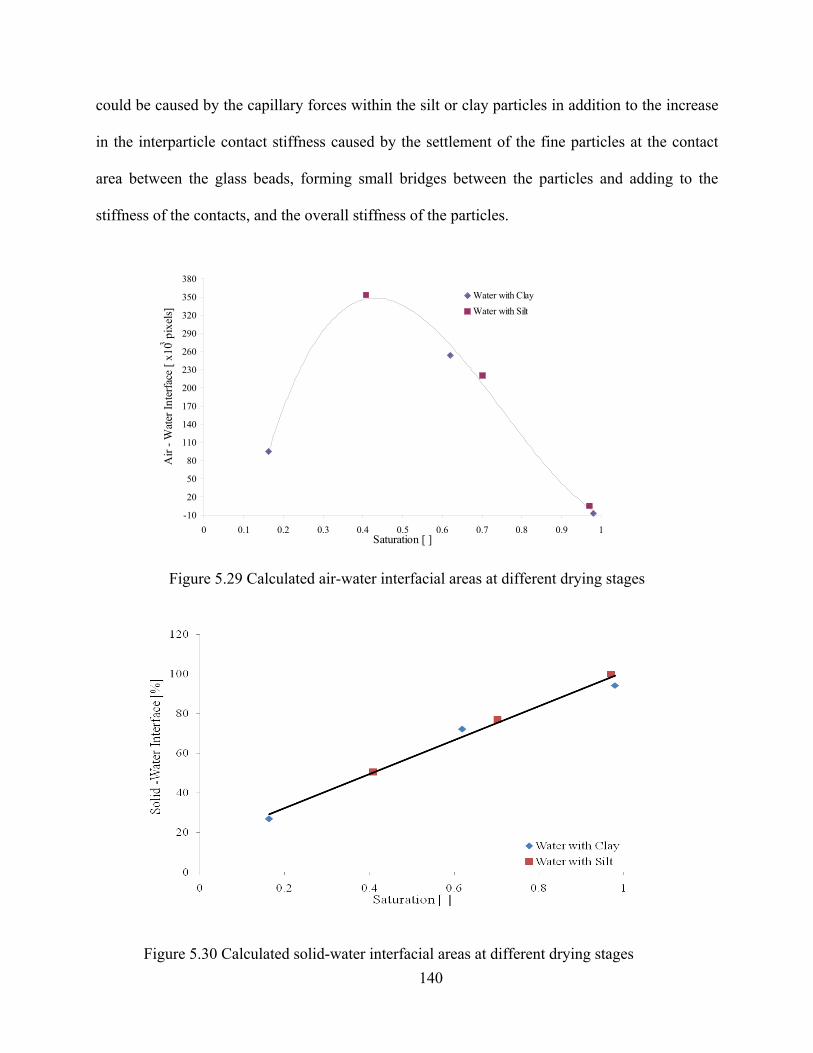
140
-10
20
50
80
110
140
170
200
230
260
290
320
350
380
0 0.1 0.2 0.3 0.4 0.5 0.6 0.7 0.8 0.9 1Saturation [ ]
Air
- Wat
er In
terfa
ce [
x103 p
ixel
s]
Water with ClayWater with Silt
could be caused by the capillary forces within the silt or clay particles in addition to the increase
in the interparticle contact stiffness caused by the settlement of the fine particles at the contact
area between the glass beads, forming small bridges between the particles and adding to the
stiffness of the contacts, and the overall stiffness of the particles.
Figure 5.29 Calculated air-water interfacial areas at different drying stages
Figure 5.30 Calculated solid-water interfacial areas at different drying stages

141
It was also shown that synchrotron X-ray tomography is a useful tool for tracking the
changes in pore fluid density at different stages of the drying process. The overall density of pore
fluid increased during drying due to the increase in the concentration of the fine silt and clay
particles, resulting in an increase of the overall stiffness of the glass beads specimen. On the
other hand, after studying the local variations in the pore fluid density it was found that the fluids
located at the interparticle contact area had a greater concentration of the fine particles than the
fluids located in pore bodies. It was also found that the air/water interfacial area steadily
increases with drying reaching a maximum value at a degree of saturation of approximately 40%.
When the water bodies are separated in the pendular regime, the interfacial area starts dropping
because of the shrinkage in the menisci causing a noticeable increase in the capillary forces and
small strain stiffness.

142
CHAPTER 6
CONCLUSIONS AND RECOMMENDATIONS
6.1 Conclusions
This dissertation presented different studies on utilizing non-destructive techniques such
as elastic and electromagnetic wave propagation as well synchrotron x-ray computed
tomography to characterize different aspects of the behavior of unsaturated soils. A new method
for the determination of field density and moisture content using elastic and electromagnetic
waves was presented. Numerical analysis and experimental studies showed that this method was
capable yielding good estimates for the soils` density and moisture content. However, various
experimental and numerical error sources resulted in some errors in the estimated density and
moisture content values. The density values were in most cases estimated with ±10% of the
measured values based on weight-volume measurements whereas the moisture content values
where estimated within ±20% of the measured values. To reduce the effects of the error sources
and to further improve the suggested methodology, a theoretical framework of a new
methodology where the S-wave velocity is added to the acquired measurements was presented.
This methodology requires a single Vp, Vs, and θv reading instead of the multiple readings
required for the original methodology. The suggested methodology and inversion algorithm will
be used to develop a prototype of a new instrument for the determination of the in situ density
and moisture content of soils. The instrument will also have the ability to monitor the small
strain stiffness on in situ soils (see Schneider, 2007) making it a very useful tool for quality
control/quality assurance of compaction projects.
On the other hand, a new apparatus was developed to monitor the changes in P- and S-
wave velocities in unsaturated soils under controlled net stress and matric suction. This apparatus

143
was used to determine the effect of matric suction on P- and S- wave velocities in soils, and to
monitor the stabilization of capillary forces process after applying different suction increments. It
was realized that increasing matric suction, caused an increase in both P- and S-wave velocities
due to the increase in the interparticle forces and therefore the overall shear stiffness. It was also
noticed that higher wave velocity values were obtained by increasing the percentage of fines in
the specimen. A theoretical model that captures the effect of both the net stress and matric
suction on the S-wave velocity was presented and was used to determine the relative effects of
the physical processes associated with saturated as well as unsaturated soils. The exponent that
represents the processes associated with unsaturated soils (βunsat) always have greater values than
the exponent that represents the nature of the interparticle contacts (β) highlighting the effect of
capillary forces on the small strain stiffness and elastic wave velocity in unsaturated soils.
The effect of the presence of fine particles in the pore fluid on the small strain stiffness of
unsaturated soils was also investigated by performing a series of drying experiments on glass
beads specimens containing different types of pore fluids while monitoring the P- and S- wave
velocities throughout the drying process. The presence of fine particles was found to have a
profound effect on the P- and S- wave velocities during drying indicating higher values of the
small strain shear, constraint, and bulk moduli. It was also found that adding a small amount of
silt or clay to the pore fluid changes the shape of the wave velocity curve during drying. These
effects are due to the increase in inter-particle contact stiffness caused by the precipitation of the
fine particles at the contact area, as well as the added capillary forces caused by the presence of
the fine particles. The results of the x-ray tomography Image analysis showed an increase in the
pore fluid density as drying proceeds indicating the migration of the fine particles to the inter-
particle contact area at lower degrees of saturation.

144
The studies presented in this dissertation aimed to highlight the significance and the great
value that elastic and electromagnetic wave measurements present for the characterization and
monitoring of the effects of different factors on the overall properties of unsaturated soils. It was
demonstrated that through monitoring the change in wave velocities, the effects of different
factors such as the volumetric water content, matric suction, and pore fluid properties could be
quantified and compared. Moreover, other important properties such as the density, moisture
content and small strain stiffness could be calculated from these measurements.
6.2 Recommendations for Future Work
The proposed methodology for the determination of density and moisture content could
be improved by eliminating or reducing the effect of the potential sources of error. The wave
velocity measurement system could be improved by using a repetitive wave source that allows
for signal stacking to eliminate the random noise in wave traces and reduce the errors in arrival
time measurements. Therefore, the use of bender elements could be a good replacement for the
drop ball method. However, the challenge here is to achieve appropriate coupling between the
bender elements and the in situ soils especially that it is difficult to imbed the bender elements in
stiff soils. Moreover, using bender elements allows for the generation of both P- and S- waves,
allowing for the implementation of the alternative methodology presented in Section 3.6. It is
also recommended that the alternative methodology should be verified by an experimental
program similar to the one performed for the original methodology. Although this methodology
theoretically presents a very promising alternative, it still needs to be experimentally verified and
tested for different types of soils to assure its proper operation.
The new triaxial apparatus could be used to perform additional experiments to determine
the effect of net stress on S- and P- wave velocities to be compared to the effect of matric
suction. A two dimensional surface could be developed combining the effects of net stress and

145
matric suction on different soil types. The experimental program could also be extended to
testing soils with different stress paths. The cell could be used to perform triaxial testing on
unsaturated soil specimens while monitoring the changes in elastic wave velocities. These tests
could also be performed at varying net stress and matric suction values to determine their relative
effects on the overall shear strength of the unsaturated soil specimens.
The effect of fine particles on the small strain stiffness could be further investigated by
testing different soil as well as different pore fluid types. Different particles shapes result in
different types of interparticle contacts, therefore, the developed drying cell could be used to
determine the effects of different factors such as particle shape, fine particle concentration and
drying rate on small strain stiffness on unsaturated soils. Moreover, synchrotron computed
tomography could be used to further investigate the properties and behavior of pore fluids during
drying as well as wetting processes.

146
REFERENCES
Aitchinson, G. D. (1961). “Relationship of Moisture and Effective Stress Functions in Unsaturated Soils.” In Pore Pressure and Suction in Soils Conference organized by British Nat. Soc. Of Int. Soc. Soil Mech. Found. Eng. And Inst. Cevil. Eng., London, England: Butterworths, pp. 47-52.
Aitchinson G. D. (ed.) (1965). “Moisture Equilibria and Moisture Changes in Soils Beneath Covered Areas.” A Symp. in Print, Australia: Buttersworth, 1965.
Alramahi, B. A., Alshibli, K. A., and Attia, A. (2006). “Influence of Grain Size and Consolidation Pressure on Porosity of Rocks.” Geotechnical Special Publication (GSP) No. 13: Site Characterization and Modeling, ASCE Geo-Frontiers Conference, Austin, Texas, January 24-26, 2005.
Alshibli, K.A., Batiste, S.N., Swanson, R.A., Sture, S., Costes, N.C., Lankton, M.R., (2000a). “Quantifying Void Ratio Variation in Sand Using Computed Tomography, Geotechnical Measurements.” Lab and Field, Proceedings of the sessions of Geo-Denver 2000, Denver, Colorado, August 5-8, 2000.
Alshibli, K.A., Sture, S., Costes, N.C., Frank, M.L., Lankton, M.R., Batiste, S.N., Swanson, R.A., (2000b). “Assessment of Localized Deformations in Sand Using X-Ray Computed Tomography.” Journal of Geotechnical Testing, 23(3), pp.274-299.
Alshibli, K. A., Abu-Farsakh, M., and Seyman, E. (2005). "Laboratory Evaluation of the Geogauge and Light Falling Weight Deflectometer as Construction Control Tools." ASCE, Journal of Materials in Civil Engineering, Vol. 17, No. 5, pp. 560-569.
Atkinson, J. H., and SÄallfors, G. (1991). “ Experimental Determination of Stress-Strain-Time Characteristics in Laboratory and In-situTests.” in Deformation of soils and displacements of structures (Proc X ECSMFE) (Ed Associazione Geo-tecnica Italiana) AA Balkema, Rotterdam, No.3, pp. 915-956.
ASTM D6758-02 (2005). “Standard Test Method for Measuring Stiffness and Apparent Modulus of Soil and Soil-Aggregate In-Place by an Electro-Mechanical Method.” ASTM International. West Conshohocken, PA.
ASTM D6780-02 (2005). “Standard Test Method for Water Content and Density of Soil in Place by Time Domain Reflectometry (TDR).” ASTM International. West Conshohocken, PA.
ASTM D1556-00 (2000). “Standard Test Method for Density and Unit Weight of Soil in Place by the Sand-Cone Method.” ASTM International, West Conshohocken, PA.
ASTM D2167-94. (1994). “Standard Test Method for Density and Unit Weight of Soil in Place by the Rubber Balloon Method.” ASTM International, West Conshohocken, PA.
ASTM D3017-04 (2004). “Standard Test Method for Water Content of Soil and Rock in Place by Nuclear Methods (Shallow Depth)." ASTM International, West Conshohocken, PA.

147
Aversa, S. and Nicotera, M. V. (2002). “A Triaxial and Oedometer Apparatus for Testing Unsaturated Soils.” ASTM Geotechnical Testing Journal, Vol. 25, No.1, pp. 3-15.
Baker, J. M. and Lascano, R. J. (1989). “The Spatial Sensitivity of Time Domain Reflectometry.” Soil Sci., Vol. 147, pp.378–384.
Balasubramonian, B. (1972). “Swelling of Compaction Shale.” PhD Thesis, Department of Civil Engineering, University of Alberta, Edmonton.
Bansal, A., Islam, M. R., (1991). “State-of-the-Art Review of Nondestructive Testing with Computer-Assisted Tomography.” SPE 22127, International Arctic Technology Conference, SPE, Anchorage, Alaska, May 29-31, 1991.
Benson, C. H. and Bosscher, P. J. (1999). “Time-Domain Refelctormetry (TDR) in Geotechnics: A Review.” Nondestructive and Automated Testing for Soil and Rock Properties. ASTM STP 1350. Edited by W. A. Marr and C. E, Fairhust. American Society of Testing and Materials. West Conshohocken, PA. pp.113-136.
Bishop, A. W. (1959). “The Principle of Effective Stress.” Lecture delivered in Oslo, Norway in 1955; Published in Teknisk Ukeblad, Vol. 106, No. 39, pp. 859-863.
Bishop, A. W., and Blight G. E. (1963). “Some Aspects of Effective Stress in Saturated and Unsaturated Soils.” Geotechnique, Vol. 13, No. 3, pp. 177-197.
Bishop, A. W. and Donald, I. B. (1961). “The Experimental Study of Partly Saturated Soil in Triaxial Apparatus.” Proc. 5th International Conference of Soil Mechanics and Foundation Engineering. Vol. 1, pp. 13-21. Paris, France.
Blewett, J., Blewett, I. J., and Woodward, P.K. (1999). “Measurement of Shear-Wave Velocity Using Phase-Sensitive Detection Techniques.” Canadian Geotechnical Journal, No. 36, pp. 934-939.
Blight, G. E. (1961). “Strength and Consolidation Characteristics of Compacted Soils.” Ph.D. dissertation, Univ. of London, London, England.
Boller, E., Cloetens, P., Baruchel, J., Tafforeau, P., Rozenbaum, O., and Pourchez, J. (2006). “Synchrotron X-ray Microtomography: A High Resolution, Fast and Quantitative Tool for Rock Characterization.” Proceedings, GeoX 2006: Advances in X-ray Tomography for Geomaterials, Aussois, France, October, 4-7 2006.
Brignoli, E. G., Gotti, M., and Stokoe, K. H. II (1996). “Measurement of Shear Waves in Laboratory Specimens by Means of Piezoelectric Transducers.” ASTM Geotechnical Testing Journal, Vol. 19, No. 4, pp. 384-397.
Burland, J. B. (1964). “Effective Stresses in Partly Saturated Soils.” Discussion of “Some Aspects of Effective stress in Saturated and Partly Saturated Soils” by G. E. Blight and A. W. Bishop. Geotechnique, Vol. 14, pp. 65-68.

148
Choi, J. S., Song, K. I., Cho, G. C. and Lee, S. W. (2004). “Characterization of Unsaturated Particulate Materials Using Elastic and Electromagnetic Waves.” Key Engineering Materials, Vols. 270-273, pp. 1653-1658.
Cho, G. C., and Santamarina, J. C. (2001). “Unsaturated Particulate Materials - Particle Level Studies.” Journal of Geotechnical and Environmental Engineering, Vol. 127, No. 1, pp. 84-96.
Coleman, J. D. (1962). “Stress/Strain Relations for Partly Saturated Soils.” Geotechnique (Correspondence), Vol 12, No. 4, pp. 348-350.
Croney, D., Coleman, J. D., and Black W. P. M. (1958). “Movement and Distribution of Water in Soil in Relation to Highway Design and Performance.” Water and Its Conduction in Soils, Highway Res. Board, Special Report, Washington, DC. No. 40, pp. 226-252.
Cromwell, V., Kortum, D. J., Bradely, D. J., (1984). “The Use of a Medical Computer Tomography (CT) System To Observe Multiphase Flow in Porous Media.” SPE 13098, 59th Annual Technical Conference and Exhibition, SPE, Houston, Texas, September 16-19, 1984
Culligan, K. A., Wildenschild, D., Christensen, B. S. B., Gray, W. G., Rivers, M., and Tompson, F. B. (2004). “Interfacial Area Measurements for Unsaturated Flow though a Porous Medium.” Water Resources Research, Vol. 40, No. 12, W12413.
Dalton F. N. and Van Genuchten M. T. (1986). “The Time Domain Reflectometry Method for Measuring Soil Water Content and Salinity.” Geoderma, Vol. 38, pp. 237-250.
Dalton, F. N, Herkelrath, W. N., Rawlins, D. S., and Rhoades, J. D. (1984). “Time Domain Reflectometry: Simultaneous Measurement of Soil Water Content and Electrical Conductivity with a Single Probe.” Science, Vol. 224. pp. 989-990.
Dalton, F.N. (1992). “Development of Time Domain Reflectometry for Measureing Soil-Water Content and Bulk Electrical Conductivity.” G. C. Topp et al.; (ed.) Advances in Measurement of Soil Physical Properties: Bringing Theory into Practice. Spec. Publ. 20. SSSA, Madison, WI. Pp. 143-167
Davis, J. and Annan, A. (1977). “Electromagnetic Detection of Soil Moisture: Progress Report 1.” Canadian Journal of Remote Sensing, Vol. 3, No.1, pp 76-86.
Desrues, J., Chambon, R., Mokni, M., Mazerolle, F., (1996). “Void Ratio Evolution Inside Shear Bands in Triaxial Sand Specimens Studied by Computed Tomography.” Geotechnique 46, No. 3, pp. 529-546.
Donald, I. B. (1961). “The Mechanical Properties of Saturated and Partly Saturated Soils with Special Reference to Negative Pore Water Pressure.” Ph.D. dissertation, Univ. of London, London, England.

149
Drnevich, V. P., Yu, Q., and Lovell, J. (2003). “Time Domain Reflectrometry for Water Content and Density of Soils: Test Procedures and Typical Results.” TRB 2003 Annual Meeting CD-ROM. National Research Council. Washington, DC. 21 pages.
Drnevich, V.P., Siddiqui, S. I., Lovell, J., and Quanghee Yi, Q. (2001). “Water Content and Density of Soil Insitu by the Purdue TDR Method.” Proceedings of the TDR2001 International Conference at Northwestern University,Evanston, Illinois, September 5-7, 2001.
Fam, M. and Santamarina, J.C. (1995). “Study of Geoprocesses with Complementary Wave Measurements in an Oedometer.” ASTM Geotechnical Testing Journal, Vol. 18, No. 3, pp. 307-314.
Fernandez, A. and Santamarina, J. C. (2001). “The Effect of Cementation on the Small Strain Parameters of Sands.” Canadian Geotechnical Journal, Vol. 38, No. 1, pp. 191-199.
Ferre, P. A., Knight, J. H., Rudolph, D. L., and Kachanoski, R. G. (1998). “The Sample Areas of Conventional and Alternative Time Domain Reflectometry Probes.” Water Resour. Res., Vol 34, pp. 2971–2979.
Fratta, D. and Santamarina, J. C. (1996). “Waveguide Device for Multi-Mode, Wideband Testing Wave Propagation in Soils.” ASTM Geotechnical Testing Journal, Vol. 19, No. 2, pp. 130-140.
Fratta D., Fernandez, A. L., and Santamarina, J. C. (2001). “Geo-Materials:Non-Destructive Evaluation in Geo-Systems.” CP557, Review of Progress in Quantitative Nondestructive Evaluation, Vol. 20, ed. by D. O. Thompson and D. E. Chimenti.
Fratta, D. and Santamarina, J. C., 2002, “Shear Wave Propagation in Jointed Rock - State of Stress.” Géotechnique, Vol. 52, No. 7, pp. 495-505.
Fratta, D., Alshibli, K. A., Tanner, W. M., and Roussel, L. (2005). “Combined TDR and P-wave Velocity Measurements for the Determination of In-Situ Soil Density.” ASTM Geotechnical Testing Journal, Vol. 26, No. 6, pp. 553-563.
Fredlund, D. G. and Rahardjo, H. (1993). “Soil Mechanics for Unsaturated Soils.” John Wily and Sons inc. 544 pages.
Fredlund, D. G., and Morgenstern, N. R. (1977). “Stress State Variables for Unsaturated Soils.” ASCE J. Geotech. Eng. Div. GT5, Vol. 103, pp. 447-466.
Giese K. and Tiemann R. (1975). “Determination of the Complex Permittivity from Thin-sample Time Domain Reflectometry Improved Analysis of the Step Response Waveform.” Advances Molecular Relaxation Processes, Vol. 7, pp. 45–59.
Gohl, W. B. and Finn W. D. L. (1991) “Use of Piezoceramic Bender Elements in Soil Dynamics Testing.” Recent Advances in Instrumentation, Data Acquisition and Testing in Soil Dynamics. ASCE Geotechnical Special Publication No. 29.

150
Hagedoorn, J. G., (1964). “The Elusive First Arrival.” Geophysics, Vol. 29, No. 5, pp. 806–813.
Ham, K. and Willson, C. (2005). “The Application of Monochromatic Energies to Investigate Multiphase Porous Media Systems using Synchrotron X-ray Tomography.” Proceeding of ASCE Geofrontiers 2005 congress, Austin, TX, January 24 – 26, 2005.
Hanks, R. J (1992). “Applied Soil Physics, Soil Water and Temperature Applications.” Springer Verlag New York Inc.
Heimovaara, T. J. (1993). “Design of Triple-Wire Time Domain Relfectometry Probes in Practice and Theory.” Soil Sci. Soc. Am. J., Vol. 59, pp. 689-698.
Herkelrath, W. N., Hamburg, S. P., and Murphy, F. (1991). “Automatic Real-Time Monitoring of Soil Moisture in a Remote Field Area with Time Domain Reflectometry.” Water Resources Res., Vol. 27, pp. 857–864.
Hilf, J. W. (1956). “An Investigation of Pore Water Pressure in Compacted Cohesive Soils.” PhD dissertation, Tech. Memo. No. 654, U.S. Dep. Of the Interior, Bureau of Reclamation, Design and Construction Div., Denver, CO.
Hook, W. R., Ferre T. P., and Livingston N. J. (2004). “The Effects of Salinity in the Accuracy and Uncertainty of Water Content Measurement.” Soil Sci. Soc. Am. J., Vol. 68., pp. 47-56.
Honarpour, M.M., Cromwell, V., Hatton, D., Satchwell, R., Reservoir Rock (1985). “Descriptions Using Computed Tomography (CT).” SPE 14272, 60th Technical Conference and Exhibition, SPE, Las Vegas, Nevada, September, 22-25, 1985.
Hoyos, L. R. and Macari, E. J. (2001). "Development of a Stress/Suction-Controlled True Triaxial Testing Device for Unsaturated Soils." Geotechnical Testing Journal, Vol. 24, No.1, pp. 5-13.
Ikeda, T. (1990). “Fundamentals of Piezoelectricity.” Oxford University. Press. Oxford. 263 pages.
Ismail, M. A., Sharma, S. S., and Fahey, M. (2005). “A Small True Triaxial Apparatus with Wave Velocity Measurement.” ASTM Geotechnical Testing Journal, Vol. 28, No. 2, pp. 113-122.
Jennings J. E. B. and Burland, J. B. (1962). “Limitations to the Use of Effective Stresses in Partly Saturated Soils.” Geotechnique, Vol. 12, No. 2. pp. 125-144.
Jennings, J. E. (1961). “A Revised Effective Stress Law for Use in the Prediction of the Behavior of Unsaturated Soils.” In Pore Pressure and Suction in Soils, conf. organized by the British Nat. Soc. Soil Mech. Found. Eng. at the Inst. Of Civil Eng. London: Buttersworth, pp. 26-30.
Jian, Z., and Jian-lin, Y. (2005). “Influences Affecting the Soil Water Characteristic Curve.” Journal of Zhejiang University Science, Vol. 6A, No. 8, pp. 797-804.

151
Jones, S. B., Wairth, J. M. and Or, D. (2001). “Time Domain Reflectometry Measurement Principles and Applications.” Hydrological Processes, Vol. 16., pp. 141-153.
Knight, J. H. (1992). “Sensitivity of Time Domain Reflectometry Measurements to Lateral Variations in Soil Water Content.” Water Resour.Res., Vol. 28., pp.2345–2352.
Krahn, J., and Fredlund, D. G., (1972). “On Total Matric and Osmotic Suction.” J. Soil. Sci., Vol. 114, No. 5, pp. 339-348.
Kramer, S. L. (1995). “Geotechnical Earthquake Engineering.” Pearson Education.
Lambe, T. W. (1960). “A Mechanistic Picture of the Shear Strength of Clay.” Proceedings of the ACSE Research Conference on the Shear Strength oh Cohesive Soils, p. 437.
Lee, J. S. and Santamarina, J. C. (2005). “Bender Elements: Performance and Signal Interpretation.” Journal of Geotechnical and Geoenvironmental Engineering, Vol. 131, No. 9, pp. 1063-1070.
Leong, E.C., Rahardjo, H. (1997). “Review of Soil-Water Characteristic Curve Equations.” Journal of Geotechnical and Geoenvironmental Engineering, Vol. 123 No. 12, pp. 1106 – 1117.
Lin, C.-P., Drnevich, V. P., Feng, W., and Deschamps, R. J. (2000). “Time Domain Reflectometry for Compaction Quality Control.” Use of Geophysical Methods in Construction, Edited by S. Nazarian and J. Diehl, Geophysical Special Publication 108, ASCE Press, pp. 15-34.
Lu, N. and Likos W. J. (2004). “Unsaturated Soil Mechanics.” John Wiley and Sons, Hoboken, New Jersey.
Lu, Z., Hickey, C. J., and Sabatier, M. (2004). “Effects of Compaction of the Acoustic Velocity in Soils.” Soil Science Society of America Journal, Vol. 68, pp. 7-16.
Macari, E. J. and Hoyos, L. R. (2001). “Mechanical Behavior of an Unsaturated Soil UnderMulti-Axial State Stress.” ASTM Geotechnical Testing Journal, Vol. 24, No. 1, pp. 14-22.
Malicki, M.A., Plagge, R., and. Roth, C.H. (1996). “Improving the Calibration of Dielectric TDR Soil Moisture Determination Taking into Account the Solid Soil.” Eur. J. Soil Sci., Vol. 47, pp. 357–366.
Matsushima, T., Uesugi, K., Nakano, K., and Tshuchiyama, A. (2006). “Visualization of Grain Motion inside a Triaxial Specimen by Micro X-ray CT at Spring-8.” Proceedings, GeoX 2006: Advances in X-ray Tomography for Geomaterials, Aussois, France, October, 4-7 2006.
Matyas, E. L. and Radhakrishna, H. S. (1968). “Volume Change Characteristics of Partially Saturated Soils.” Geotechnique, Vol. 18. No. 4, pp. 432-448.

152
Mavko, G., Mukerji, T., and Dvorkin, J. (1998). “The Rock Physics Handbook.” Cambridge University Press. 329 pages.
Miller, C.J., Yesiller, N., Yaldo, K., and Merayyan, S. (2002). “Impact of Soil Type and Compaction Conditions on Soil Water Characteristic.” Journal of Geotechnical and Geoenvironmental Engineering, Vol. 128, No. 9, pp. 773 – 742.
Mitarai, N. and Nori, F. (2006). “Wet Granular Materials.” Advances in Physics, Vol. 55, Nos. 1-2, pp. 1-45.
Mithcell, J. K. (1962). “Components of Pore Water Pressure and Their Engineering Significance.” Proceedings of the Ninth National Clay Conference, Clays and Clay Minerals, pp. 162-184.
Mithcell, J. K. (1993). “Fundamentals of Soil Behavior.” John Wiley and Sons Inc.
Mojid, M., Wyseure, G., and Rose, D. (1998). “The use of Insulated Time Domain Reflectometry Sensors to Measure Water Content in Highly Saline Soils.” Irrigation Science, Vol. 18, pp. 55-61.
Mojid, M., Wyseure, G., Rose, D. (2003). “Electrical Conductivity Problems Associated with Time Domain Reflectometry (TDR) Measurement in Geotechnical Engineering.” Geotechnical and Geological Engineering, Vol. 21, pp. 243-258.
Morgenstern, N. R. (1979). “Properties of Compacted Soils.” Contribution to Panel Discussion, Session IV, Proc. of the 6th Pan-American Conf. Soil Mech. Found. Eng. (Lima, Peru), Vol. 3, December 1979, pp. 349 – 354.
Multiquip, inc. (2004). “Soil Compaction, a Basic Handbook.” Multiquip, inc., Carson, CA.
Nadler, A., Dasberg, S., and Lapid, I. (1991). “Time Domain Reflectometry Measurements of Water Content and Electrical Conductivity of Layered Soil Columns.” Soil Sci. Soc. Am. J., Vol. 55, pp. 938-943.
Nadler, A., Gamliel, A., and Peretz, I. (1999). “Practical Aspects of Salinity Effect on TDR Measured Water Content: A Field Study.” Soil Sci. Soc. Am. J., Vol. 63, pp. 1070-1076.
Nichol C., Beckie, R., and Smith, L. (2002). “Evaluation of Uncoated Time Domain Reflectometry Probes for High Electrical Conductivity Systems.” Soil Sci. Soc. Am. J., Vol. 66, pp. 1454-1465.
Nielsen, D.C., Lagae, H. J., and Anderson, R. L. (1995). “Time Domain to Obtain the Apparent Dielectric Constant from Time Domain. Reflectometry Measurements of Surface Soil Water Content.” Soil Sci. Soc. Am. J., Vol. 59, pp. 103–105.
Noborio, K., McInnes K. J., and Heilman, J. L. (1994). “Field Measurements of Soil Water Content and Electrical Conductivity By Time Domain Reflectometry.” Comput. Electron. Agric., Vol. 11, pp. 131-142.

153
Noborio, K. (2001). “Measurement of Soil Water Content and Electrical Conductivity by Time Domain Reflectometry: A Review.” Computers and Electronics in Agriculture, Vol. 31, pp. 213-237.
O’Connor, K. M. and Dowding, C. H. (1999). “Geomeasurements by Pulsing TDR Cables and Probes.” CRC Press LLC. 402 pages.
Otani, J., Mukunoki, T., Obara, Y., (2000). “Application of X-Ray CT Method for Characterization of Failure in Soils.” Soils and Foundations, Vol. 40, No. 2, 111-118.
Otani, J. (2006). “X-ray Computed Tomography for Geotechnical Engineering.” Proceedings, GeoX 2006: Advances in X-ray Tomography for Geomaterials, Aussois, France, October, 4-7 2006.
Persson, M. and Wraith, J. (2002). “Shaft Mounted Time Domain Reflectometry Probe for Water Content and Electrical Conductivity Measurements.” Vadose Zone Journal, Vol. 1, pp. 316-319.
Petersen L. W., Thomsen, A., Moldrup, P., Jacobsen, O. H., and Rolston, D., E. (1995). “High Resolution Time Domain Reflectometry: Sensitivity Dependency on Probe Design.” Soil Sci., Vol. 159, pp.149–154.
Piezo system, inc. (2005). Company website (url: http://www.piezo.com).
Porras-Ortiz, O. F. (2004). “Small and Large Strain Monitoring of Unsaturated Soil Behavior by Means of Multiaxial Testing and Shear Wave Propagation.” PhD Dissertation. Louisiana State University. Baton Rouge, LA.
Qian, X., Gray, D. H., and Woods, R. D. (1991). “Resonant Column Tests on Partially Saturated Sands.” ASTM Geotechnical Testing Journal, Vol. 14, No. 3, pp. 266-275.
Qian, X., Gray, D. H., and Woods, R. D. (1993). “Voids and Granulometry: Effects on Shear Modulus of Unsaturated Sands.” Journal of Geotechnical Engineering, Vol. 119, No. 2, pp. 296-314.
Richards, B. G. (1966). “The Significance of Moisture Flow and Equilibria in Unsaturated Soils in Relation to the Design on Engineering Structures Built on Shallow Foundations an Australia.” Presented on the Symposium on Permeability and Capillary, Amer Soc. Testing Materials, Atlantic City, NJ.
Richart, F. E., Hall, J. R., and Woods, R. D. (1970). “Vibrations Soils and Foundations.” Prentice-Hall. Englewood Cliffs, NJ. 414 pages.
Rivers, M. L., Sutton, S. R., and Eng, P. (1999). “Geoscience Applications of X-ray Computed Microtomography.” In Ulrich Bonse (ed.) Developments in X-ray Tomography II. Proc. SPIE Vol. 3772. SPIE, Bellingham, WA, pp. 78–86.

154
Robinson D., Jones, S., Wraith, J., and Friedman, S. (2003). “A Review of Advances in Dielectric and Electrical Conductivity Measurement in Soils Using Time Domain Reflectometry.” Vadose Zone Journal Vol. 2, pp. 444-475.
Robinson, D.A., and S.P. Friedman (2000). “Parallel Plates Compared to Conventional Rods as TDR Waveguides for Sensing Soil Moisture.” Subsurface Sens. Technol. Appl., Vol. 1, pp. 497–511.
Roessler, S. (1979). “Anisotropic Shear Modulus Due to Stress Anisotropic.” Journal of the Geotechnical Engineering Division, Vol. 150, No. GT7, pp. 871-880.
Sanchez-Salinero, I., Roesset, J. M., and Stokoe, K. H. (1986). “Analytical Studies of Body Wave Propagation and Attenuation.” Report GR 86-15, Civil Engineering Department, University of Texas at Austin, TX.
Santamarina, J. C., Rinaldi, V. A., Fratta, D., Klein, K. A., Wang. Y.-H., Cho, G.-C., and Cascante, G. (2005). “A Survey of Elastic and Electromagnetic Properties of Near-Surface Soils.” Near-Surface Geophysics, Ed. D. Buttler, SEG. pp. 71-87.
Santamarina, J. C., Klein, K. A., and Fam, M. A. (2001). “Soils and Waves.” John Wiley & Sons, LTD. New York. 488 pp.
Santamarina, J. C., Rinaldi, V. A., Fratta, D., Klein, K. A., Wang. Y.-H., Cho, G.-C., and Cascante, G. (2005). “A Survey of Elastic and Electromagnetic Properties of Near-Surface Soils.” Near-Surface Geophysics, Ed. D. Buttler, SEG .
Sawangsuriya, A., (2006). “Stiffness-Suction-Moisture Relationship for Compacted Soils.” Ph.D. Dissertation. University of Wisconsin-Madison. Madison, WI.
Sawangsuriya, A., Bosscher, P. J., and Edil, T. B. (2003). “Laboratory Evalaution of the Soil Stiffness Gauge.” Transportation Research Record 1808, pp. 30-37.
Sawangsuriya, A., Edil, T. B., and Bosscher, P. J. (2004). “Assessing Small-strain Stiffness of Soils Using the Soil Stiffness Gauge.” Proceedings of the 15th Southeast Asian Geotechnical Society Conference, Bangkok, Thailand, pp.101-106.
Sawangsuriya, A., Biringen, E., Fratta, D., Bosscher, P. J. and Edil, T. B. (2006). “Dimensionless Limits for the Collection and Interpretation of Wave Propagation Data in Soils.” ASCE Geotechnical Special Publication (GSP) 149: “Site and Geomaterial Characterization”. Edited by A. Puppala, D., Fratta, K. Alshibli, and S. Pamucku., pp. 160-166.
Siddiqui, S. I. and V. P. Drnevich (1995). A New Method of Measuring Density and Moisture Content of Soil Using the Technique of Time Domain Reflectometry, Report No: FHWA/IN/JTRP-95/9.” Joint Transportation Research Program, Indiana Department of Transportation-Purdue University, February 1995, 271 pages.
Shirley, D. J. and Hampton, L. D. (1978) “Shear Wave Measurements in Laboratory Sediments.” Journal of Acoustics Society of America, Vol. 63, No. 2, pp. 607-613.

155
Silva, C. H. C., Porras-Ortiz, O. F., Fratta, D., and Macari, E. J. (2002). “Mechanical Response of Unsaturated Particulate Materials – A Stiffness Assessment Study under Controlled Matric Suction.” Proceedings of the ASME International Mechanical Engineering Congress & Exposition. New Orleans, LA, November 17-22
Skempton, A. W. (1960). “Effective Stress in Soil, Concrete, and Rocks.” Proceedings of the Conference on Pore Pressure and Suction in Soils, pp. 4-16.
Stokoe, K. H., Lee, J. N.-K., and Lee, S. H.-H. (1991). “Characterization of Soil in Calibration Chambers with Seismic Waves.” - Proceedings of the Symposium in Calibration Chamber Testing, 1991.
Terzaghi, K. (1936). “The Shear Resistance of Saturated Soils.” Proceedings of the 1st International Conference of Soil Mechanics and Foundation Engineering, Vol. 1, pp. 54-56.
Thomann, T. G. and Hryciw, R. D. (1990). “Laboratory Measurement of Small Strain Shear Modulus Under Ko Conditions.” ASTM Geotechnical Testing Journal, Vol. 13, No. 2. pp. 97-105.
Topp, G. C., Davis, J. L., and Annan, A. P. (1980). “Electromagnetic Determination of Soil Water Content: Measurements in Coaxial Transmission Lines.” Water Resources Research, Vol. 16, No. 3, pp 574-582.
Topp, G. C. and Davis, J. L. (1985). “Time Domain Reflectometry (TDR) and Its Applications to Irrigation Scheduling.” Advances in Irrigation, Vol. 3, pp. 107-127.
TransTech (2005). TransTech Company Web Site. URL: www.transtechsys.com
Van Genuchten, M. T. (1980). “A Closed-form Equation for Predicting the Hydraulic Conductivity of Unsaturated Soils.” Soil Science Society Science of America Journal, Vol. 44, pp. 892-898.
Vinale, F., D’Onofrio, A. Mancuso, C. Santicci de Magistris, F. and Tatsuoka, F. (2001). “The Pre-Failure of Soils as Construction Materials, Pre-Failure Deformation Characteristics of Geomaterials.” pp. 955-1007.
Vogeler, I., Clothier, B. E., Green, S. R., Scotter, D. R., and Tillman, R. W. (1996). “Characterizing Water and Solute Movement by Time Domain Reflectometry and Disk Permeametry.” Soil Sci. Soc. Am. J., Vol. 60., pp. 5–12.
Weast. R. C., Astle, M. J., and Beyer, W. H. (1981). “CRC Handbook of Chemistry and Physics” 65th edition, Boca Raton, Fl.
White, J. E. (1983). “Underground Sound. Application of Seismic Waves.” Elsevier. Amsterdam.253 pages.

156
Wildenschild, D., Hopmans, J. W., Rivers, M. L., and Kent, A. J. R. (2005). “Quantitative Analysis of Flow Processes in a Sand Using Synchrotron-Based X-ray Microtomography.” Vadose Zone Journal, Vol. 4, pp. 112-126.
Wood, D. M. (2004). “Geotechnical Modeling.” Spon Press (UK), 488 pages.
Wu, S., Gray, D. H., and Richart, F. E. (1984). “Capillary Effects on Dynamic Modulus of Sands and Silts.” Journal of Geotechnical Engineering, Vol. 110, No. 9, pp. 1188-1203.
Wyseure G. C. L., Mojid M. A., and Malik M. A. (1997). “Mesurement of Volumetric Water Content by TDR in Saline Soils.” Eur. J. of Soil Sci. 48. pp. 347 – 354.
Yang, H., Rahardjo, H., Leong, E. C., and Fredlund, D. G. (2004). “Factors Affecting Drying and Wetting Soil-Water Characteristic Curves of Sandy Soils.” Canadian Geotechnical Journal, No. 41, pp. 908-920.
Yu, X. and Drnevich, V. P. (2004). “Soil Water Content and Dry Density by Time Domain Reflectometer.”, Journal of Geotechnical and Geoenvironmental Engineering, Vol. 130, No. 9, pp. 922-934.
Zegelin S., White, I., and Jenkins D., (1989). “Improved Field Probes for Soil Water Content and Electrical Conductivity Measurements using Time Domain Reflectometry.” Water Resources Research, Vol. 25, No. 11, pp. 2367-2376.

157
VITA
Bashar Alramahi was born on September of 1979, in Beirut, Lebanon. He attended high
school at Al-Ittihad School in Amman, Jordan, and graduated in 1997. He then moved to
Ramallah, Palestine, where he attended Birzeit University and received his bachelor`s degree in
civil engineering in August, 2002. He came to the United States in January, 2003 and started his
graduate studies at Louisiana State University in Baton Rouge, Louisiana. He obtained a
master`s degree in geotechnical engineering in August, 2004. He is expected to receive the
degree of Doctor of Philosophy in geotechnical engineering in December, 2007. He currently
works as a research assistant professor at Southern University - Baton Rouge performing levee
analysis and design tasks as part of the recovery efforts in New Orleans, Louisiana, after
hurricane Katrina.