Embed Size (px)
Citation preview

Centre for Geotechnical and Materials Modellinghttp://livesite.newcastle.edu.au/cgmm/1/66
Daichao SHENG
The University of Newcastle, Australia
General Report5th International Conference on Unsaturated Soils
6-8 Sept, 2010, Barcelona, Spain
Constitutive Modelling of Unsaturated Soils: Discussion of Fundamental Principles

Centre for Geotechnical and Materials Modellinghttp://livesite.newcastle.edu.au/cgmm/2
Outline
1. Introduction
2. Volume change behaviour of unsaturated soils
3. Yield stress versus suction relationship
4. Shear strength of unsaturated soils
5. Hydro-mechanical coupling for unsaturated soils
6. Implementation of unsaturated soil models into FEM
7. Concluding remarks

Centre for Geotechnical and Materials Modellinghttp://livesite.newcastle.edu.au/cgmm/3
(Li, 2010)
1. Introduction: Fundamental Issues
Volume change caused by suction change
(Gens, 2007 ← Viggiani)

Centre for Geotechnical and Materials Modellinghttp://livesite.newcastle.edu.au/cgmm/4
1. Introduction: Fundamental Issues
Shear strength change caused by suction change
Zhou-Qu Landslide (8-8-2010, Gansu, China)
Thredbo Landslide (30-7-1997, NSW, Australia)

Centre for Geotechnical and Materials Modellinghttp://livesite.newcastle.edu.au/cgmm/5
1. Introduction: Fundamental Issues
MINE WASTE
UNSATURATED SOIL LAYERS
Flow of moisture, oxygen, heat,…
Hydraulic properties of unsaturated soils
Centre for Geotechnical and Materials Modellinghttp://livesite.newcastle.edu.au/cgmm/6
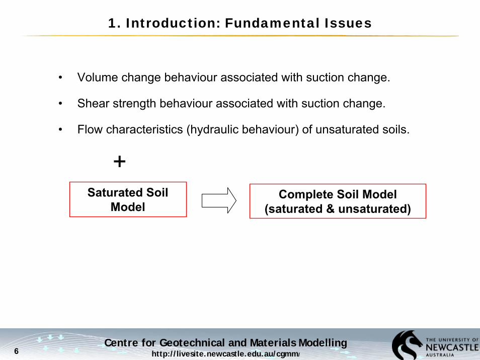
1. Introduction: Fundamental Issues
• Volume change behaviour associated with suction change.
• Shear strength behaviour associated with suction change.
• Flow characteristics (hydraulic behaviour) of unsaturated soils.
Saturated Soil Model
Complete Soil Model (saturated & unsaturated)
+

Centre for Geotechnical and Materials Modellinghttp://livesite.newcastle.edu.au/cgmm/7
s
1. Introduction: BBM (Alonso, Gens & Josa, 1990)
Modified Cam Clay model (saturated soil) + shear strength vs suction
+ volume change vs suction
q
ap p u= −
Loading-collapse surface ↔ volume
Zero shear strength line

Centre for Geotechnical and Materials Modellinghttp://livesite.newcastle.edu.au/cgmm/8
1. Introduction: BBM (Alonso, Gens & Josa, 1990)
BBM (Alonso et al, 1990):
1. It is the very first complete model that accommodates the key fundamental issues of unsaturated soils.
2. BBM’s seminal contributions: treating suction as an additional variable in the stress space and using the Loading-Collapse (LC) yield surface to model wetting-induced volume collapse.
3. It has inspired many researchers to unsaturated soil mechanics. Numerous other models have since been developed.

Centre for Geotechnical and Materials Modellinghttp://livesite.newcastle.edu.au/cgmm/9
State-of-the-art reviews on constitutive modelling of unsaturated soils:
1. Gens (1st Int. Conf. Unsat. Soils, Paris, 1995)
2. Wheeler & Karube (1st Int. Conf. Unsat. Soils, Paris, 1995)
3. Alonso (2nd Int. Conf. Unsat. Soils, Beijing, 1998, expansive soils)
4. Fredlund (3rd Int. Conf. Unsat. Soils, Recife, 2002, hydraulic)
5. Vaunat (1st MUSE School, Barcelona, 2005)
6. Wheeler (4th Int. Conf. Unsat. Soils, Arizona, 2006)
7. Gens (1st European Conf. Unsat. Soils, Durham, 2008)
8. Gens (4th Asian-Pacific Conf. Unsat. Soils, Newcastle, 2009)
9. Gens (47th Rankine Lecture, Geotechnique, 2010)
This report focuses on a selected number of fundamental issues.
1. Introduction: State-of-Art Reports

Centre for Geotechnical and Materials Modellinghttp://livesite.newcastle.edu.au/cgmm/10
Outline
1. Introduction
2. Volume change behaviour of unsaturated soils
3. Yield stress versus suction relationship
4. Shear strength of unsaturated soils
5. Hydro-mechanical coupling for unsaturated soils
6. Implementation of unsaturated soil models into FEM
7. Concluding remarks
Alternative methods

Centre for Geotechnical and Materials Modellinghttp://livesite.newcastle.edu.au/cgmm/11
2. Volume Change Behaviour: Saturated Soils
Saturated, normally consolidated soil:
N=3, λ=0.2,
sae>100kPa
Normally consolidated
1.5
2.0
2.5
3.0
1 10 100 1000
uw=0
uw=-10 kPa
uw=-100 kPa
v
lnp
( )wln lnv N p N p uλ λ′= − = − −
w
w w
d( )dd upvp u p u
λ λ −= − −
− −

Centre for Geotechnical and Materials Modellinghttp://livesite.newcastle.edu.au/cgmm/12
2. Volume Change Behaviour: Unsaturated Soils
Saturated NC soils:
Approach A. Separate stress and suction approach (net stress and suction approach: Alonso et al. 1990; Wheeler & Sivakumar 1995; Cui & Delage 1996; ….)
Approach B. Combined stress-suction approach (effective stress approach: Kohgo et al 1993; Bolzen et al 1996; Loret & Khalili 2002; Sheng et al 2003, 2004; Sun et al. 2006; …)
Approach C. A more recent approach (SFG approach: Sheng, Fredlund & Gens, 2008)
Unsaturated soils?
w
w w
d( )dd upvp u p u
λ λ −= − −
− −
( )wln lnv N p N p uλ λ′= − = − −

Centre for Geotechnical and Materials Modellinghttp://livesite.newcastle.edu.au/cgmm/13
Separate stress and suction (net stress and suction) approach:
Advantage: the compressibilities due to stress and suction changes are handled separately.
2. Volume Change Behaviour: Approach A
atvp vs
at
( ) ln ln s uv N s pu
λ λ⎛ ⎞+
= − − ⎜ ⎟⎝ ⎠
Toll (1990)
Toll & Ong (2003)
λ(Sr=1)
λvp
λvs
Centre for Geotechnical and Materials Modellinghttp://livesite.newcastle.edu.au/cgmm/14
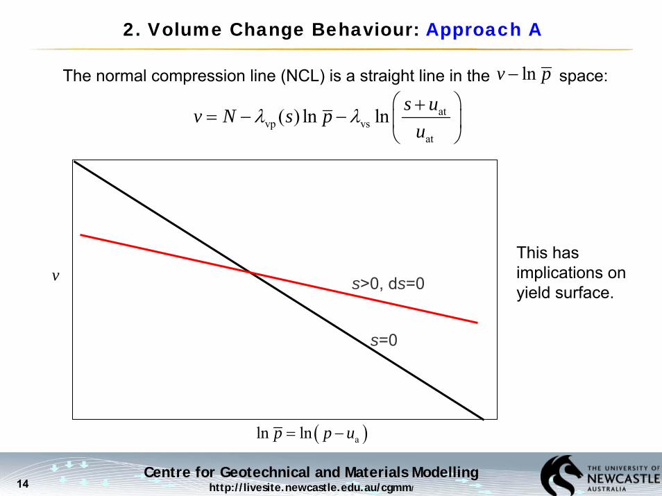
The normal compression line (NCL) is a straight line in the space:
2. Volume Change Behaviour: Approach A
atvp vs
at
( ) ln ln s uv N s pu
λ λ⎛ ⎞+
= − − ⎜ ⎟⎝ ⎠
s>0, ds=0
s=0
v
( )aln lnp p u= −
This has implications on yield surface.
lnv p−

Centre for Geotechnical and Materials Modellinghttp://livesite.newcastle.edu.au/cgmm/15
The volume change is not well defined at the transition suction. For a stress change from to :
in unsaturated zone
in saturated zone
Implications on the zero shear strength (apparent tensile strength) surface.
2. Volume Change Behaviour: Approach A
ae
aevp
0 ae
Δ lns
p svp s
λ−
+= −
+
aevp
0
Δ lns
pvp
λ+ = −
0p p

Centre for Geotechnical and Materials Modellinghttp://livesite.newcastle.edu.au/cgmm/16
Combined stress-suction (effective stress) approach:
2. Volume Change Behaviour: Approach B
s>0, ds=0
( )ln ( ) ln ( )v N p N s p f sλ λ′= − = − +
s=0
lnp
v
ln p
Advantage:
1. NCL is curved in space.
2. It recovers the saturated soil model.
lnv p−

Centre for Geotechnical and Materials Modellinghttp://livesite.newcastle.edu.au/cgmm/17
Difficult to handle the different compressibilities due to stress and suction changes
2. Volume Change Behaviour: Approach B
Toll (1990)
Toll & Ong (2003)
λ(Sr=1)
λvp
λvs

Centre for Geotechnical and Materials Modellinghttp://livesite.newcastle.edu.au/cgmm/18
2. Volume Change Behaviour: Approach B
( )ln ( ) ln ( )v N p N s p f sλ λ′= − = − +
1
Alternative forms of Approach B
NA
B
s=0
s>0
v
Drying path
ln p′
( ) 1(0)sλ
λ<
Centre for Geotechnical and Materials Modellinghttp://livesite.newcastle.edu.au/cgmm/19
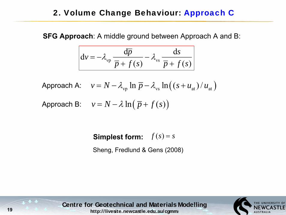
2. Volume Change Behaviour: Approach C
vp vsd dd
( ) ( )p sv
p f s p f sλ λ= − −
+ +
SFG Approach: A middle ground between Approach A and B:
( )f s s=Simplest form:
( )vp vs at atln ln ( ) /v N p s u uλ λ= − − +
( )ln ( )v N p f sλ= − +
Approach A:
Approach B:
Sheng, Fredlund & Gens (2008)
Centre for Geotechnical and Materials Modellinghttp://livesite.newcastle.edu.au/cgmm/20
0.1
0.3
0.5
0.7
0.9
1.1
1 10 100 1000 10000
NCL: s=10 kPa
NCL: s=0 kPa
2.00
1.46
1.01
0.65
0.35
0.11
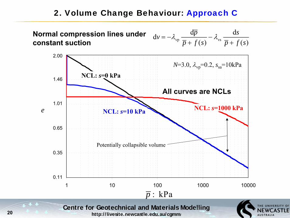
Potentially collapsible volume
2. Volume Change Behaviour: Approach C
Normal compression lines under constant suction
N=3.0, λvp=0.2, ssa=10kPa
e
: kPap
All curves are NCLs
vp vsd dd
( ) ( )p sv
p f s p f sλ λ= − −
+ +
NCL: s=1000 kPa

Centre for Geotechnical and Materials Modellinghttp://livesite.newcastle.edu.au/cgmm/21
2. Volume Change Behaviour: Approach C
Volume change caused by suction change: vp vs
d dd =( ) ( )
p svp f s p f s
λ λ− −+ +
0.20
0.40
0.60
0.80
1.00
1.20
1 10 100 1000 10000s (kPa)
e
2.32
1.72
1.23
0.82
0.49
0.22
=100 kPap
=1 kPap
=10 kPap
=1000 kPap
VO
ID R
ATI
O
0.90
0.80
0.70
0.60
0.50
0.401 10 100 1000
SUCTION (kPa)
E1 NC 25 kPa
E2 NC 50 kPa
E7 NC 200 kPa
E11 NC 400 kPa
E5 OC 200 kPa
E6 OC 800 kPa
Vicol. (1990)

Centre for Geotechnical and Materials Modellinghttp://livesite.newcastle.edu.au/cgmm/22
2. Volume Change Behaviour: Approach C
s (kPa)
Prediction of SFG model
1 10 100 1000 10000 100000
0.84
0.83
0.82
0.81
0.80
0.79
0.78
e
Air-dry silt: Data from Jennings and Burland (1962)
vp sa
vs savp sa
s ss s ss
λλ
λ
≤⎧⎪= ⎨
>⎪⎩

Centre for Geotechnical and Materials Modellinghttp://livesite.newcastle.edu.au/cgmm/23
2. Volume Change Behaviour: Approach C
Compacted expansive clay: Sivakuma and Wheeler (2000)
(kPa)
Yield stress
NCL by Approach A
NCL by SFG model
v
△ s = 0○ s = 300 kPa
10 100 1000
2.25
2.20
2.15
2.10
2.05
2.00
1.95
Unloading-reloading line
p
Centre for Geotechnical and Materials Modellinghttp://livesite.newcastle.edu.au/cgmm/24
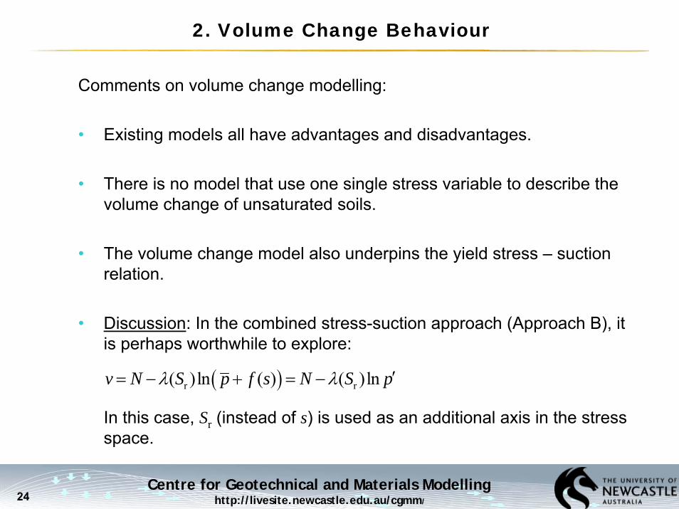
2. Volume Change Behaviour
Comments on volume change modelling:
• Existing models all have advantages and disadvantages.
• There is no model that use one single stress variable to describe the volume change of unsaturated soils.
• The volume change model also underpins the yield stress – suction relation.
• Discussion: In the combined stress-suction approach (Approach B), it is perhaps worthwhile to explore:
In this case, Sr (instead of s) is used as an additional axis in the stress space.
( )r r( )ln ( ) ( )lnv N S p f s N S pλ λ ′= − + = −

Centre for Geotechnical and Materials Modellinghttp://livesite.newcastle.edu.au/cgmm/25
Outline
1. Introduction
2. Volume change behaviour of unsaturated soils
3. Yield stress versus suction relationship
4. Shear strength of unsaturated soils
5. Hydro-mechanical coupling for unsaturated soils
6. Implementation of unsaturated soil models into FEM
7. Concluding remarks

Centre for Geotechnical and Materials Modellinghttp://livesite.newcastle.edu.au/cgmm/26
3. Yield Stress vs Suction: Approach A
Isotropic Compression Curves
v=1+e
ln p
s=0
s1
s2
s3
0<s1 < s2 < s3
pc1 < pc2 < pc3
c1p c2p c3p

Centre for Geotechnical and Materials Modellinghttp://livesite.newcastle.edu.au/cgmm/27
3. Yield Stress vs Suction: Approach A
p
s
s3
s2
s1
Loading-collapse yield surface (LC)
Zero shear strength
(Apparent tensile strength, ATS)
Suction Increase (SI)
pc1p c2p c3p

Centre for Geotechnical and Materials Modellinghttp://livesite.newcastle.edu.au/cgmm/28
3. Yield Stress vs Suction: Soils reconstituted from slurry
Variation of yield stress with suction
Stress path B’D is elastoplastic, not purely elastic.
s
Initialelastic zone
p
D
45oA E F G
B'
B yield surface evolution
Centre for Geotechnical and Materials Modellinghttp://livesite.newcastle.edu.au/cgmm/29
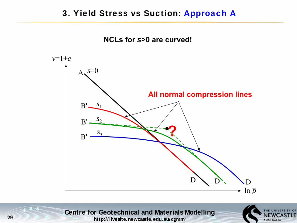
3. Yield Stress vs Suction: Approach A
NCLs for s>0 are curved!
v=1+e
ln p
s=0
s1
s2
s3
All normal compression lines
?
A
B'
B'
B'
D D D

Centre for Geotechnical and Materials Modellinghttp://livesite.newcastle.edu.au/cgmm/30
0
100
200
300
400
500
600
700
800
900
1000
-400 -300 -200 -100 0 100 200 300 400 500 600p (kPa)
A
B
45o
0p cBp
s
Initial elastic zone
3. Yield vs Suction: Approach C (SFG)
Evolution of yield surface during drying and compression
cDp
A
B
p
s
D
ATSSI
LC
D

Centre for Geotechnical and Materials Modellinghttp://livesite.newcastle.edu.au/cgmm/31
3. Yield Stress vs Suction: Approach B (Effective Stress)
Evolution of yield surface in effective stress space
s
p′A
zero shear strength line: 0p′ =
45o
B
B' D
ABB' : Drying under 0p =
B'D: elastoplastic
SI LC
( ) ( ) lnv N s s pλ ′= −
?
ATS

Centre for Geotechnical and Materials Modellinghttp://livesite.newcastle.edu.au/cgmm/32
3. Yield Stress vs Suction
Comments on yield stress – suction relationship:
• The yield stress – suction relationship is embedded in the volume change model.
• The zero shear strength (ATS) surface, the suction-increase (SI) surface and the loading-collapse (LC) surface are related to each other. In effective stress models and in the SFG model, the SI and LC surfaces are all evolved from the zero shear strength surface.
Centre for Geotechnical and Materials Modellinghttp://livesite.newcastle.edu.au/cgmm/33
Outline
1. Introduction
2. Volume change behaviour of unsaturated soils
3. Yield stress versus suction relationship
4. Shear strength of unsaturated soils
5. Hydro-mechanical coupling for unsaturated soils
6. Implementation of unsaturated soil models into FEM
7. Concluding remarks

Centre for Geotechnical and Materials Modellinghttp://livesite.newcastle.edu.au/cgmm/34
4. Shear Strength of Unsaturated Soils
In a critical state constitutive model, the shear strength of the soil is fully defined by:- The slope of the critical state line M(s) (or the friction angle φ) and - The zero shear strength function, 0 ( )p s
0 ( )p s
p
s
45 o
q
CSL
M(s)
CSL
M(s)

Centre for Geotechnical and Materials Modellinghttp://livesite.newcastle.edu.au/cgmm/35
4. Shear Strength of Unsaturated Soils
Bishop & Blight (1963):
Fredlund et al (1978):
( )n tan tanc s cτ σ χ φ σ φ′= + + = +
bn tan tanc sτ σ φ φ= + +
0( )p s
Volume change

Centre for Geotechnical and Materials Modellinghttp://livesite.newcastle.edu.au/cgmm/36
or
Pereira & Alonso (2009)
0
500
1000
1500
2000
0 200 400 600 800 1000 1200 1400
Suction (kPa)
Dev
iato
r stre
ss (k
Pa)
4. Shear Strength of Unsaturated Soils
Various shear strength equations used to define χ or φb
Predictions
Test data (after Cunningham et al, 2003)
2
1
5
3
46 8
7 To capture the peak value:
( )rSχ χ=
( )reSχ χ=
( )b brSφ φ=

Centre for Geotechnical and Materials Modellinghttp://livesite.newcastle.edu.au/cgmm/37
4. Shear Strength of Unsaturated Soils
The slope of CSL (M) or the friction angle (φ):
Some experimental data support that M or φ does not depend on suction (Ng & Chiu, 2004; Thu et al 2007; Nuth & Laloui 2008)
Nuth & Laloui (2008)
Mean net stress (kPa)
Dev
iato
r stre
ss (k
Pa)
Suct
ion
(kPa
)
Thu et al (2007)

Centre for Geotechnical and Materials Modellinghttp://livesite.newcastle.edu.au/cgmm/38
4. Shear Strength of Unsaturated Soils
Some data support that the friction angle (φ) depends on suction or degree of saturation (Toll, 1990; Merchán et al 2008)
Merchán et al (2008)
Toll & Ong (2003)
Centre for Geotechnical and Materials Modellinghttp://livesite.newcastle.edu.au/cgmm/39
4. Shear Strength of Unsaturated Soils
Comment on shear strength of unsaturated soils:
• If the friction angle (φ) is independent of suction, all existing shear strength equations can be formulated in terms of a single effective stress. The real challenge is to find an effective stress when φdepends on suction.

Centre for Geotechnical and Materials Modellinghttp://livesite.newcastle.edu.au/cgmm/40
Outline
1. Introduction
2. Volume change behaviour of unsaturated soils
3. Yield stress versus suction relationship
4. Shear strength of unsaturated soils
5. Hydro-mechanical coupling for unsaturated soils
6. Implementation of unsaturated soil models into FEM
7. Concluding remarks

Centre for Geotechnical and Materials Modellinghttp://livesite.newcastle.edu.au/cgmm/41
5. Hydro-Mechanical Coupling: SWCC & Its Hysteresis
Sr
lns
sI
sD
s0
1
Main drying curve
Main wetting curve
A
BC
D
B’ C’
D’
Soil water characteristic (or retention) curve, SWCC or SWRC
Scanning curves

Centre for Geotechnical and Materials Modellinghttp://livesite.newcastle.edu.au/cgmm/42
5. Hydro-mechanical Coupling: VRJ Model
Vaunat, Romero & Jommi Model (2000)
lns
ELASTIC ZONE
SI Surface: Drying
SD Surface: Wetting
ln p
LC Surface: Loading
Centre for Geotechnical and Materials Modellinghttp://livesite.newcastle.edu.au/cgmm/43
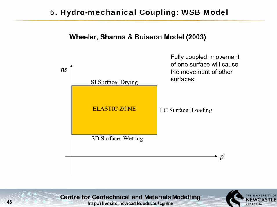
5. Hydro-mechanical Coupling: WSB Model
Wheeler, Sharma & Buisson Model (2003)
ns
ELASTIC ZONE
SI Surface: Drying
SD Surface: Wetting
p′
LC Surface: Loading
Fully coupled: movement of one surface will cause the movement of other surfaces.

Centre for Geotechnical and Materials Modellinghttp://livesite.newcastle.edu.au/cgmm/44
5. Hydro-mechanical Coupling: SSG Model
Sheng, Sloan & Gens Model (2004)
s
ELASTIC ZONE
SI Surface: Drying
SD Surface: Wetting
p′
LC Surface: Loading
The movement of SI & SD surfaces are not coupled with the movement of LC surface.
Centre for Geotechnical and Materials Modellinghttp://livesite.newcastle.edu.au/cgmm/45
5. Hydro-mechanical Coupling: Density Effect on SWCC
The density effect on SWCC (Sun et al, 2007b):
(1) The shift of SWCC as the initial void ratio of the soil changes,(2) The volume change along SWCC, or(3) The change of degree of saturation caused by loading/unloading
when the suction is kept constant.

Centre for Geotechnical and Materials Modellinghttp://livesite.newcastle.edu.au/cgmm/46
5. Hydro-mechanical Coupling: Density Effect on SWCC
In the literature, the change of degree of saturation is often attributed to the change of suction and the change of soil volume, in a form as:
……………………………(29)
This has been used in Sheng et al. (2004); Sun et al. (2007b); Nuth & Laloui (2008a); Mašín (2010); Nuth & Laloui (2008b); Khalili et al. (2008); ….
Note: SWCC is usually obtained under constant stress, not constant volume. Suction change (ds) will also cause volume change (dεv).
( ) ( )r vd d dS s ε= +
Centre for Geotechnical and Materials Modellinghttp://livesite.newcastle.edu.au/cgmm/47
5. Hydro-mechanical Coupling: Density Effect on SWCC
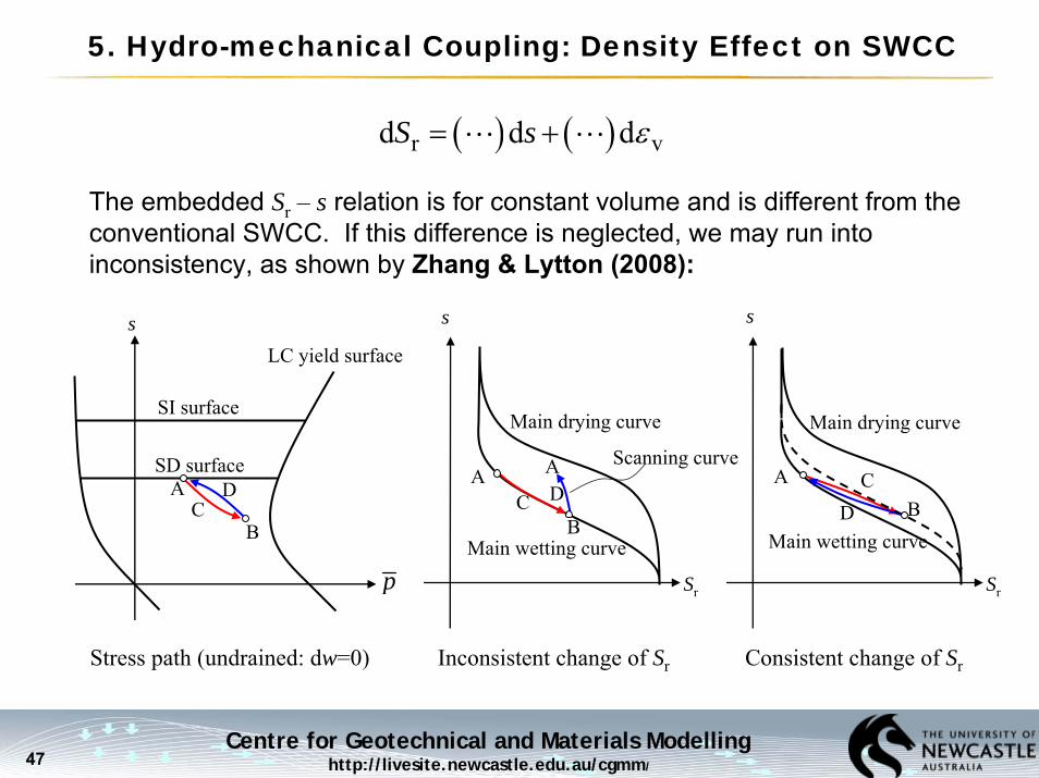
The embedded Sr – s relation is for constant volume and is different from the conventional SWCC. If this difference is neglected, we may run into inconsistency, as shown by Zhang & Lytton (2008):
( ) ( )r vd d dS s ε= +
Stress path (undrained: dw=0) Inconsistent change of Sr Consistent change of Sr
A
B
Main drying curve
Main wetting curve
s
Sr
C D
Scanning curveA AB
Main drying curve
Main wetting curve
s
Sr
CD
A
B
LC yield surface
SI surface
SD surface
s
CD
p

Centre for Geotechnical and Materials Modellinghttp://livesite.newcastle.edu.au/cgmm/48
?
5. Hydro-mechanical Coupling: Density Effect on SWCC
Alternative way to formulate the hydraulic equation:
where de0 is the change of void ratio purely due to stress change.
There are constraints on the Sr – e relationship:
Sheng & Zhou (2010)
( ) ( ) ( ) ( )r 0d d d d dS SWCC s p SWCC s e= + = +
r r r1S S Se e e
− ∂ −≤ ≤
∂
rr r0, when 1 or 0S S S
e∂
= = =∂
r r r
0 0
(1 )S S Se e
β∂ −= −
∂
rrd d , when d 0SS e w
e= − =

Centre for Geotechnical and Materials Modellinghttp://livesite.newcastle.edu.au/cgmm/49
5. Hydro-mechanical Coupling: Density Effect on SWCC
This approach is comparable with Gallipoli et al (2003b) where the van Genuchten equation is modified to account for void ratio effect:
This modified VG equation can also be written as:
r r r
0 0
(1 )S S Se e
β∂ −= −
∂
1/r r r
0 0
(1 )mS S Smne e
ψ∂ −= −
∂
( )r
0
1
1
m
nSe sψφ
⎡ ⎤⎢ ⎥=⎢ ⎥+⎣ ⎦
c.f.
= 1 Sheng & Zhou (2010)
Centre for Geotechnical and Materials Modellinghttp://livesite.newcastle.edu.au/cgmm/50
5. Hydro-mechanical Coupling: Density Effect on SWCC
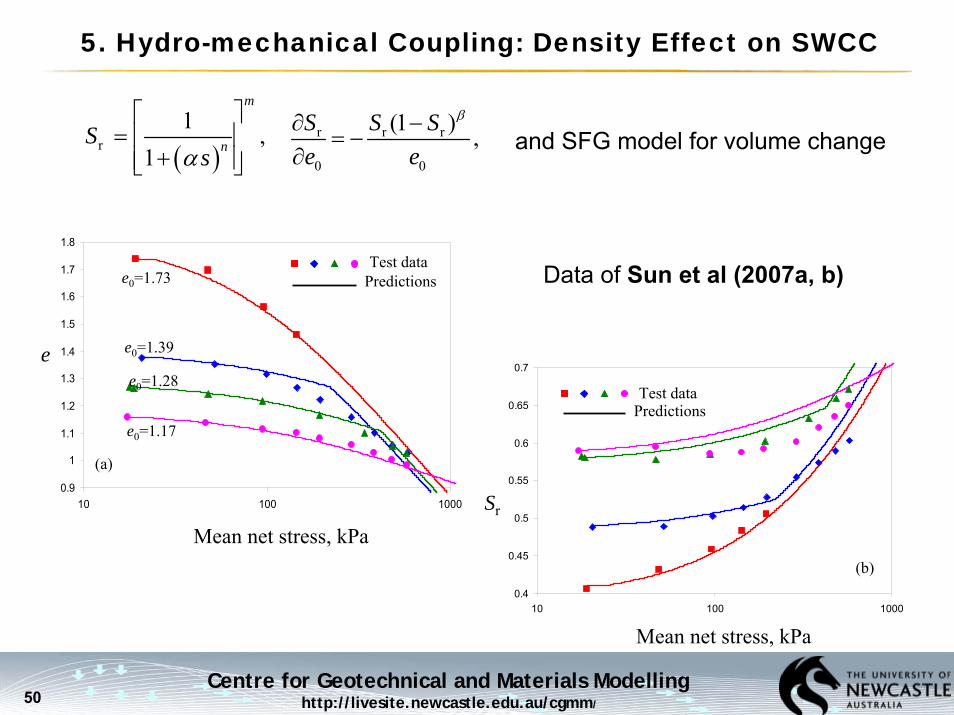
Data of Sun et al (2007a, b)
r r r
0 0
(1 ) ,S S Se e
β∂ −= −
∂( )r1 ,
1
m
nSsα
⎡ ⎤= ⎢ ⎥
+⎢ ⎥⎣ ⎦
0.9
1
1.1
1.2
1.3
1.4
1.5
1.6
1.7
1.8
10 100 1000
Mean net stress, kPa
e
Test dataPredictionse0=1.73
e0=1.39
e0=1.28
e0=1.17
(a)
0.4
0.45
0.5
0.55
0.6
0.65
0.7
10 100 1000
Mean net stress, kPa
Sr
Test dataPredictions
(b)
and SFG model for volume change
Centre for Geotechnical and Materials Modellinghttp://livesite.newcastle.edu.au/cgmm/51
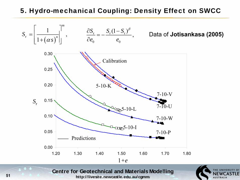
5. Hydro-mechanical Coupling: Density Effect on SWCC
Data of Jotisankasa (2005)r r r
0 0
(1 ) ,S S Se e
β∂ −= −
∂( )r1 ,
1
m
nSsα
⎡ ⎤= ⎢ ⎥
+⎢ ⎥⎣ ⎦
0.00
0.05
0.10
0.15
0.20
0.25
0.30
1.20 1.30 1.40 1.50 1.60 1.70 1.80
Sr
1+e
7-10-U
Calibration
7-10-V
7-10-P
7-10-W
5-10-K
5-10-L
5-10-I
Predictions

Centre for Geotechnical and Materials Modellinghttp://livesite.newcastle.edu.au/cgmm/52
5. Hydro-mechanical Coupling: Density Effect on SWCC
Data of Sharma (1998)r r r
0 0
(1 ) ,S S Se e
β∂ −= −
∂( )r1 ,
1
m
nSsα
⎡ ⎤= ⎢ ⎥
+⎢ ⎥⎣ ⎦
Sr
0.60
0.70
0.80
0.90
1.00
1.10
1.50 1.70 1.90 2.10 2.30 2.501+ e
s=100kPa
s=200kPas=300kPa
Calibration curve
Predictions
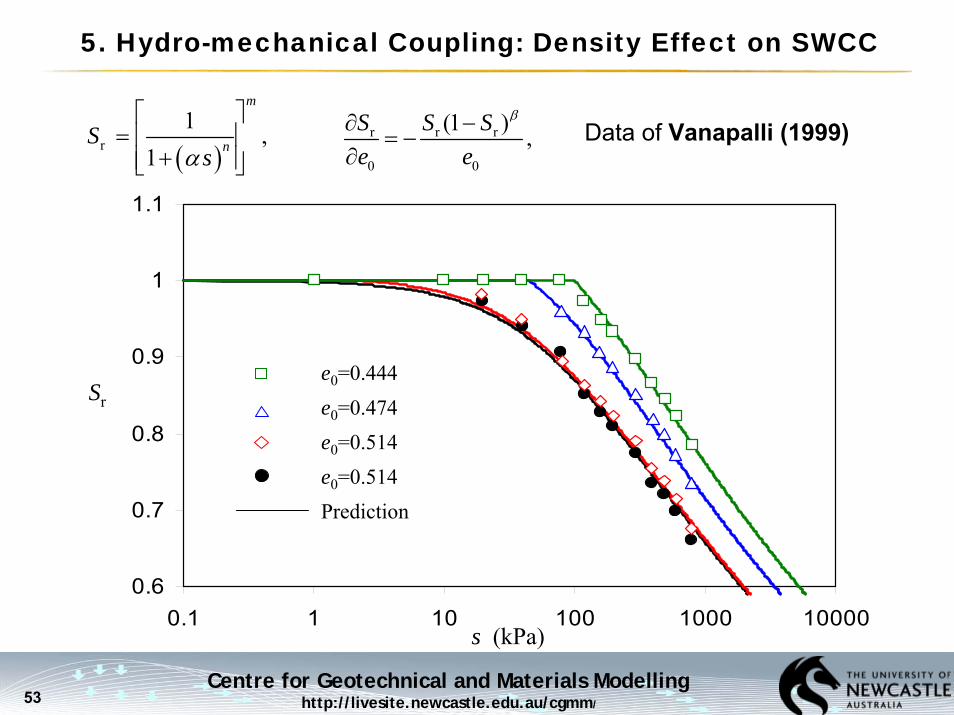
Centre for Geotechnical and Materials Modellinghttp://livesite.newcastle.edu.au/cgmm/53
0.6
0.7
0.8
0.9
1
1.1
0.1 1 10 100 1000 10000
5. Hydro-mechanical Coupling: Density Effect on SWCC
Data of Vanapalli (1999)r r r
0 0
(1 ) ,S S Se e
β∂ −= −
∂( )r1 ,
1
m
nSsα
⎡ ⎤= ⎢ ⎥
+⎢ ⎥⎣ ⎦
s (kPa)
e0=0.444e0=0.474e0=0.514e0=0.514Prediction
Sr

Centre for Geotechnical and Materials Modellinghttp://livesite.newcastle.edu.au/cgmm/54
5. Hydro-mechanical Coupling: Density Effect on SWCC
Data of Tarantino (2009)r r r
0 0
(1 ) ,S S Se e
β∂ −= −
∂( )r1 ,
1
m
nSsα
⎡ ⎤= ⎢ ⎥
+⎢ ⎥⎣ ⎦
0.50
0.60
0.70
0.80
0.90
1.00
1.10
10 100 1000 10000s (kPa)
e0=0.62
e0=0.54
e0=0.50
Prediction
Sr

Centre for Geotechnical and Materials Modellinghttp://livesite.newcastle.edu.au/cgmm/55
5. Hydro-mechanical Coupling: Density Effect on SWCC
Comment on hydro-mechanical coupling:
• The conventional soil-water characteristic curve (or soil-water retention curve) is obtained under constant stress, not constantvolume. This must be considered in the hydro-mechanical coupling.
Centre for Geotechnical and Materials Modellinghttp://livesite.newcastle.edu.au/cgmm/56
Outline
1. Introduction
2. Volume change behaviour of unsaturated soils
3. Yield stress versus suction relationship
4. Shear strength of unsaturated soils
5. Hydro-mechanical coupling for unsaturated soils
6. Implementation of unsaturated soil models into FEM
7. Concluding remarks

Centre for Geotechnical and Materials Modellinghttp://livesite.newcastle.edu.au/cgmm/57
6. Implementation of Constitutive Model: Non-Convexity
s
p
Net stress – suction space: BBM
Elastic zone
Centre for Geotechnical and Materials Modellinghttp://livesite.newcastle.edu.au/cgmm/58
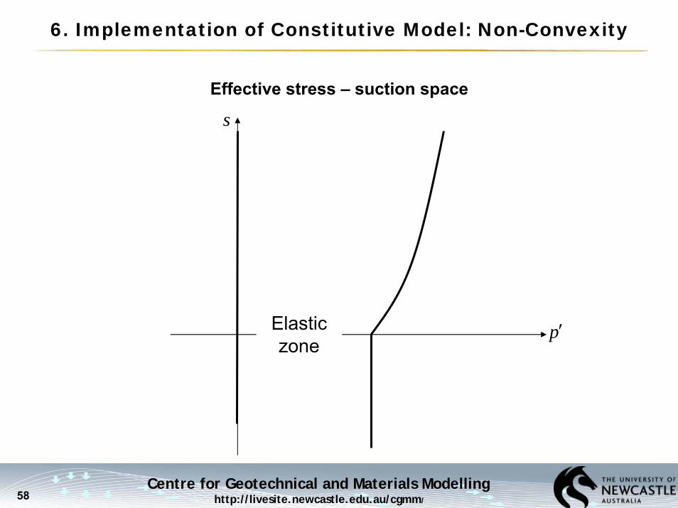
6. Implementation of Constitutive Model: Non-Convexity
s
p′
Effective stress – suction space
Elastic zone

Centre for Geotechnical and Materials Modellinghttp://livesite.newcastle.edu.au/cgmm/59
6. Implementation of Constitutive Model: Non-Convexity
Challenge:
An elastic trial stress path with both the starting and ending stress states inside the elastic zone can cause plastic yielding.
s
p
A
B
Centre for Geotechnical and Materials Modellinghttp://livesite.newcastle.edu.au/cgmm/60
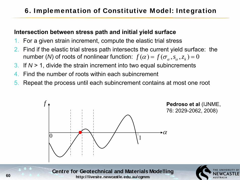
6. Implementation of Constitutive Model: Integration
Intersection between stress path and initial yield surface1. For a given strain increment, compute the elastic trial stress2. Find if the elastic trial stress path intersects the current yield surface: the
number (N) of roots of nonlinear function:3. If N > 1, divide the strain increment into two equal subincrements4. Find the number of roots within each subincrement5. Repeat the process until each subincrement contains at most one root
f
α
( ) ( , , ) 0kf f s zα αα σ= =
0 1
Pedroso et al (IJNME, 76: 2029-2062, 2008)

Centre for Geotechnical and Materials Modellinghttp://livesite.newcastle.edu.au/cgmm/61
6. Implementation of Constitutive Model: Integration
Number of Roots
The number (N) of roots of nonlinear function
f: yield functiong: first order derivative of fh: second order derivative of f
( ) ( , , ) 0kf f s zα αα σ= =
[ ]( )2
2 2 2 2
( ) ( ) ( ) ( )( ) ( ) ( ) 1d arctan( ) ( ) ( ) ( ) ( ) ( )
b
a
f a g b f b g af h gNf g f a f b g a g b
γγ α α α απ α γ α π γ
⎧ ⎫−− − ⎪ ⎪= + ⎨ ⎬+ +⎪ ⎪⎩ ⎭∫
Kronecker–Picard formula (Kavvadias et al, 1999)
It is computationally expensive to estimate N

Centre for Geotechnical and Materials Modellinghttp://livesite.newcastle.edu.au/cgmm/62
6. Implementation of Constitutive Model: Integration
Numerical Example: Integration of the SFG model
Sheng et al (Comput. Mech., 42: 685-694, 2008b)
p
s
0 20 40 60 80 100
020
4060
8010
0
Centre for Geotechnical and Materials Modellinghttp://livesite.newcastle.edu.au/cgmm/63
7. CONCLUDING REMARKS
1. Partial saturation is a state of soil and any soil be unsaturated with water. Models for unsaturated soils should be able to deal with arbitrary suction and stress changes within possible pore pressures and stress ranges.
2. The volume change equation is one of the most fundamental properties for unsaturated soils. It underpins the yield stress – suction and shear strength – suction relationships.
3. When coupling the hydraulic component with the mechanical component in a constitutive model, it is recommended to take into account the volume change along soil-water characteristic curves.
Centre for Geotechnical and Materials Modellinghttp://livesite.newcastle.edu.au/cgmm/64
7. CONCLUDING REMARKS
4. The volume change of unsaturated soils can not easily be described by one single stress variable.
5. On the other hand, there is little difference in formulating shear strength equations in one single stress variable or in two independent stress variables, if the friction angle is assumed to be independent of suction.
6. Unsaturated soil models are characterised by non-convex yield surfaces near the transition between saturated and unsaturated states. This non-convexity, if handled rigorously, can significantly complicate the implementation of these models into finite element codes.

Centre for Geotechnical and Materials Modellinghttp://livesite.newcastle.edu.au/cgmm/65
Gens (2008, Durham)
+ + +BBM SFG

Centre for Geotechnical and Materials Modellinghttp://livesite.newcastle.edu.au/cgmm/66
ACKNOWLEDGEMENT
A number of people have read the draft paper and provided valuable comments:YJ Cui, DG Fredlund, D Gallipoli, SL Houston, J Kodikara, DM Pedroso, JM Pereira, WT Solowski, DA Sun, C Yang, X Zhang, AN Zhou
The work presented in the paper involves important contributions from:DG Fredlund, A Gens, DM Pedroso, DA Sun and AN Zhou
Australian Research Council has provided financial support for research on unsaturated soils at Newcastle.
THANK YOU ALL

Centre for Geotechnical and Materials Modellinghttp://livesite.newcastle.edu.au/cgmm/67
2. Volume Change Behaviour: Approach B vs C
vp vsd dd
( ) ( )p sv
p f s p f sλ λ= − −
+ +
Approach C (SFG):
Approach B (effective stress):
Approach C recovers Approach B only if:
Therefore, Approach B is more constraint than Approach C.
( )ln ( )v N p f sλ= − +
vs vpddfs
λ λ=

Centre for Geotechnical and Materials Modellinghttp://livesite.newcastle.edu.au/cgmm/68
2. Volume Change Behaviour: Unsaturated Soils
Isotropic compression curves for reconstituted soils
Jennings & Burland(1962)

Centre for Geotechnical and Materials Modellinghttp://livesite.newcastle.edu.au/cgmm/69
2. Volume Change Behaviour: Unsaturated Soils
Isotropic compression curves for compacted soils
Wheeler & Sivakumar(2000)

Centre for Geotechnical and Materials Modellinghttp://livesite.newcastle.edu.au/cgmm/70
2. Volume Change Behaviour: Gallipoli et al (2003a)
Isotropic compression curves for compacted soils
Gallipoli et al(2003a), data of Sharma (1998)
Centre for Geotechnical and Materials Modellinghttp://livesite.newcastle.edu.au/cgmm/71
2. Volume Change Behaviour: Romero & Jommi (2010)
Isotropic compression curves for compacted soils
Romero & Jommi (2010)

Centre for Geotechnical and Materials Modellinghttp://livesite.newcastle.edu.au/cgmm/72
2. Volume Change: Approach B
( )( ) ( ) ln ( )v N s s p f sλ= − +
Why can’t we shift the NCLs upwards in the v – lnp' space?
N(s)
A
NCL(s=0)
NCL(s>0)
v
Drying path under constant p'?
N(0)
ln p′
v
p′
s
A
Drying under constant p':
Zero shear strength line
Compression under constant s (elastic)
?
Where is the expansion of the elastic zone?

Centre for Geotechnical and Materials Modellinghttp://livesite.newcastle.edu.au/cgmm/73
ln p′1
A
B
s>0
v
s=0
N Drying path under constant p
2. Volume Change: Approach B
Alternative forms of Approach B
( )r( )ln ( )v N S p f sλ= − +
Al-Badran & Schanz (2009)
Sr
p′
LC surface
Zero
she
ar
stre
ngth
line
( ) r
(1)( )
c c0Sp p
λ κλ κ
−−′ ′=

Centre for Geotechnical and Materials Modellinghttp://livesite.newcastle.edu.au/cgmm/74
Questions
2. Why should the loading-collapse yield surface recover the apparent tensile strength surface when pc(s=0)=0?
s
pslurry (v=N)
s
p′slurry45o
• The zero shear strength line must be unique.• The LC surface is evolved from this slurry line.
Centre for Geotechnical and Materials Modellinghttp://livesite.newcastle.edu.au/cgmm/75
s
p′
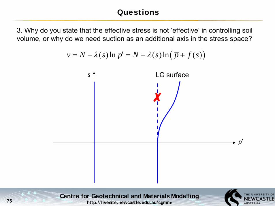
Questions
✘
3. Why do you state that the effective stress is not ‘effective’ in controlling soil volume, or why do we need suction as an additional axis in the stress space?
( )( ) ln ( ) ln ( )v N s p N s p f sλ λ′= − = − +
LC surface
Centre for Geotechnical and Materials Modellinghttp://livesite.newcastle.edu.au/cgmm/76
Questions
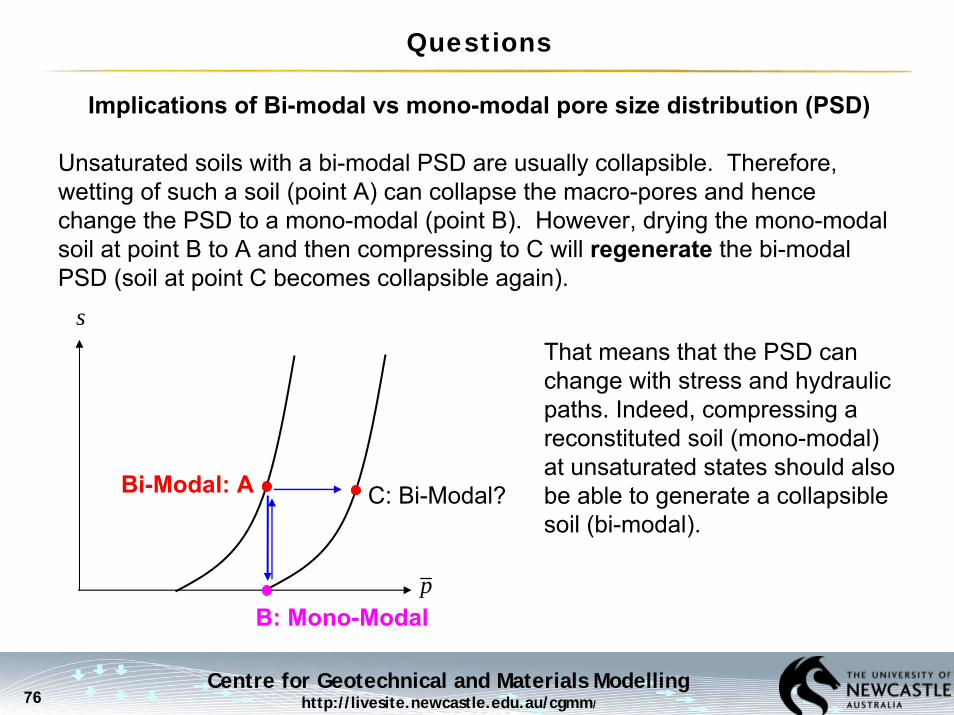
Implications of Bi-modal vs mono-modal pore size distribution (PSD)
Unsaturated soils with a bi-modal PSD are usually collapsible. Therefore, wetting of such a soil (point A) can collapse the macro-pores and hence change the PSD to a mono-modal (point B). However, drying the mono-modal soil at point B to A and then compressing to C will regenerate the bi-modal PSD (soil at point C becomes collapsible again).
Bi-Modal: A
B: Mono-Modal
s
p
That means that the PSD can change with stress and hydraulic paths. Indeed, compressing a reconstituted soil (mono-modal) at unsaturated states should also be able to generate a collapsible soil (bi-modal).
C: Bi-Modal?

Centre for Geotechnical and Materials Modellinghttp://livesite.newcastle.edu.au/cgmm/77
Questions
4. In a critical state model, should the critical state shear strength depend on hydraulic hysteresis? In other words, two samples of the same soil are sheared under exactly the same suction, the mean net stress and the same void ratio, but different degrees of saturation. Should its critical state strength be different?
o Implications: Is it necessary to have both Sr and s in the shear strength and volume change equations?
o Pros: Some data seem to show such differences in CS strength (e.g. Sun et al. 2010).
o Cons: CS shear strength is less dependent on the initial conditions of the sample (e.g. OCR, water content, void ratio, initial structure, cementation, …) for saturated soils. An unsaturated soil model can not be better than its base model for saturated states.

Centre for Geotechnical and Materials Modellinghttp://livesite.newcastle.edu.au/cgmm/78
Questions
Implications of the maximum shear strength at intermediate suctions (SFG)
s
p45o
Zero shear strength line
v
lns
vp sa
vs savp sa
SFG: s s
s s ss
λλ
λ
≤⎧⎪= ⎨
>⎪⎩ ?s
q

Centre for Geotechnical and Materials Modellinghttp://livesite.newcastle.edu.au/cgmm/79
s
p
Stress Path Dependency in Elastic Zone (SFG Model)
Arbitrary yield surface
A (p0, s0)
D (p, s)B
C
evp vs
d dd p svp s p s
κ κ= − −+ +
evp vp vp
d( ) d dd p s p svp s p s p s
κ κ κ+= − = − −
+ + +
evpABD
Δ ln(36.9)v κ= −
evpACD
Δ ln(38.2)v κ= −
0 0
sa
11, 10 (kPa) 20, 20, 10 (kPa)
p sp s s
= = −= = =
vpe evp vpABD ACD
vp
ln1.0338.2Δ Δ ln( ) ln1.03, 0.008 0.8%36.9 ln 36.9
v vκ
κ κκ
−− = − = − = =
−
unsaturated
saturated

Centre for Geotechnical and Materials Modellinghttp://livesite.newcastle.edu.au/cgmm/80
s
p
Stress Path Dependency in Elastic Zone (Model A)
Arbitrary yield surface
A (p0, s0)
D (p, s)B
C
evp vs
d dd p svp s
κ κ= − −
evp vs
at
d dd p svp s u
κ κ= − −+
evp vp vp
d( ) d dd p s p svp s p s p s
κ κ κ+= − = − −
+ + +
evpABD
Δ ln(76.4)v κ= −
evpACD
Δ ln(60)v κ= −
0 0
sa
11, 10 (kPa) 20, 20, 10 (kPa)
p sp s s
= = −= = =
vpe evp vpABD ACD
vp
ln1.2776.4Δ Δ ln( ) ln1.27, 0.06 6%60 ln 60
v vκ
κ κκ
−− = − = − = =
−
unsaturated
saturated
Centre for Geotechnical and Materials Modellinghttp://livesite.newcastle.edu.au/cgmm/81
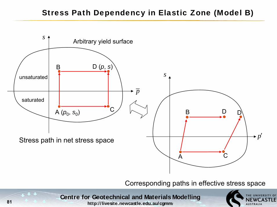
Stress Path Dependency in Elastic Zone (Model B)
s
p
Arbitrary yield surface
A (p0, s0)
D (p, s)B
C
unsaturated
saturated
s
p′
Corresponding paths in effective stress space
A
DB
C
D
Stress path in net stress space

Centre for Geotechnical and Materials Modellinghttp://livesite.newcastle.edu.au/cgmm/82
Work-Conjugate Stress and Strain Variables
Work Input (Houlsby, 1997):
( ) ar w r a r r a
a(1 ) (1 )ij ij ij ijW S u S u n s S n S u ρσ δ δ ε
ρ= − − − + + −
( ) ( )
( )
( )
aa r w a r r a
a
aa r v r r a
a
aa r a
a
(1 )
(1 )
(1 )
ij ij ij ij ij
ij ij ij
ij ij ij
W u S u u nsS n S u
u S s nsS n S u
u s n S u
ρσ δ ε δ ερ
ρσ δ ε ερ
ρσ δ ε θρ
= − − − + + −
= − + + + −
= − + + −

Centre for Geotechnical and Materials Modellinghttp://livesite.newcastle.edu.au/cgmm/83
Work-Conjugate Stress and Strain Variables
( ) ( )a a w w q 0 rd d d d dw p u p u q n s Sϕ ϕ ε= − + − + −
Work Input (Coussy, Pereira & Vaunat, 2010)
With two non-connected saturating fluids:
With connected fluids:
( )a v r v q rd d d d dw p u S s q n s Sε ε ε= − + + −
Centre for Geotechnical and Materials Modellinghttp://livesite.newcastle.edu.au/cgmm/84
SFG Modelling Approach
Volumetric Model →
Hardening Law →
Yield Stress →
Shear Strength
SFG model (Sheng, Fredlund and Gens, Canadian Geotechnical Journal, 45(4), 511-523, 2008)
Centre for Geotechnical and Materials Modellinghttp://livesite.newcastle.edu.au/cgmm/85
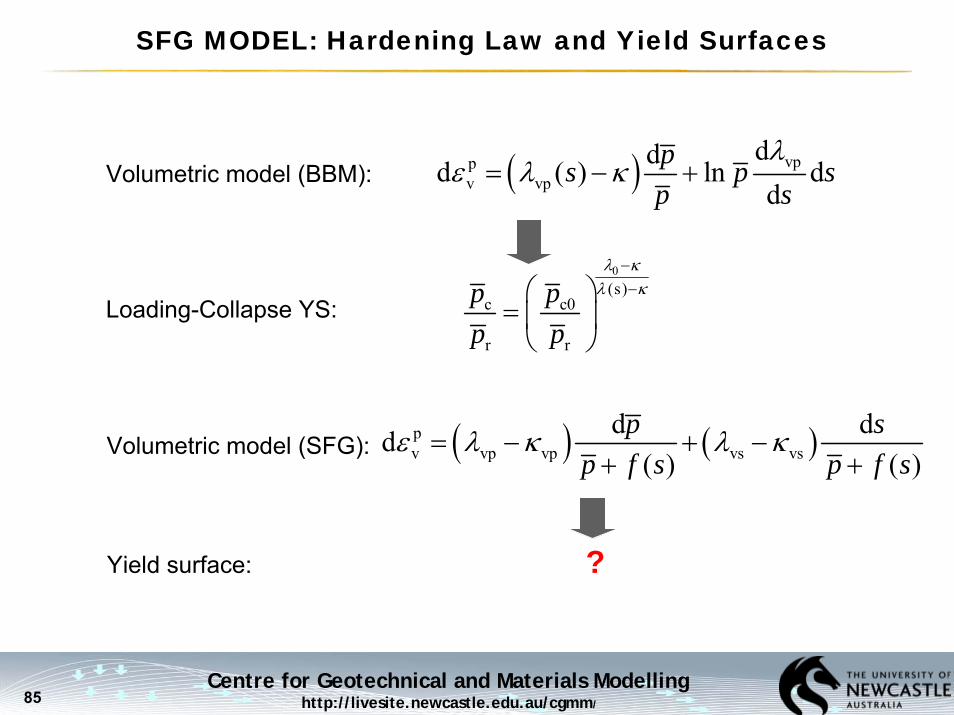
SFG MODEL: Hardening Law and Yield Surfaces
Volumetric model (BBM): ( ) vppv vp
ddd ( ) ln dd
ps p sp s
λε λ κ= − +
0(s)
c c0
r r
p pp p
λ κλ κ
−−⎛ ⎞
= ⎜ ⎟⎝ ⎠
Loading-Collapse YS:
( ) ( )pv vp vp vs vs
d dd( ) ( )
p sp f s p f s
ε λ κ λ κ= − + −+ +
Volumetric model (SFG):
Yield surface: ?

Centre for Geotechnical and Materials Modellinghttp://livesite.newcastle.edu.au/cgmm/86
c0 sa
cc0 sa sa sa
saln
p s s sp sp s s s s
s
− <⎧⎪= ⎨ − − ≥⎪⎩
0
100
200
300
400
500
600
700
800
900
1000
-400 -300 -200 -100 0 100 200 300 400 500 600
0p
p
s
(kPa)
Initial elastic zone
cBp
ssa
B
c0p
SFG MODEL: Hardening Law and Yield Surfaces
Initial yield surface and its evolution during compaction
cDp
cn0 sa
cn cn0c0 sa sa sa
c0 saln
p s s sp p sp s s s s s s
p s
− <⎧⎪= ⎛ ⎞⎨ + − − − ≥⎜ ⎟⎪
⎝ ⎠⎩
cn0p
A
B
p
s
DATS SI
LC
D
Centre for Geotechnical and Materials Modellinghttp://livesite.newcastle.edu.au/cgmm/87
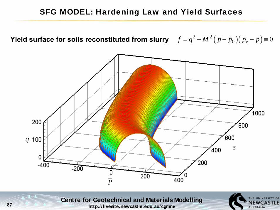
SFG MODEL: Hardening Law and Yield Surfaces
Yield surface for soils reconstituted from slurry
p
sq
( )( )2 20 c 0f q M p p p p= − − − ≡

Centre for Geotechnical and Materials Modellinghttp://livesite.newcastle.edu.au/cgmm/88
SFG MODEL: Hardening Law and Yield Surfaces
Yield surface for a compacted soil
p
q
s
( )( )2 20 c 0f q M p p p p= − − − ≡

Centre for Geotechnical and Materials Modellinghttp://livesite.newcastle.edu.au/cgmm/89
0
100
200
300
400
500
600
700
800
900
1000
-400 -300 -200 -100 0 100 200 300 400 500 600
5. Hydro-mechanical Coupling: SFG Model
Sheng, Gens & Fredlund (2008)
0p
s
(kPa)
ELASTIC ZONE
SI: Drying
SD: Wetting
cp
p

Centre for Geotechnical and Materials Modellinghttp://livesite.newcastle.edu.au/cgmm/90
2. Volume Change Behaviour: Approach C
s (kPa)1 10 100 1000 10000 100000
1.54
1.52
1.50
1.48
1.46
1.44
1.42
v
Reconstituted silty clay: Data from Cunningham et el. (2003)
Prediction of SFG model
vp sa
vs savp sa
s ss s ss
λλ
λ
≤⎧⎪= ⎨
>⎪⎩
Centre for Geotechnical and Materials Modellinghttp://livesite.newcastle.edu.au/cgmm/91
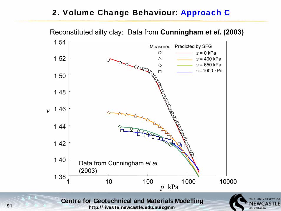
2. Volume Change Behaviour: Approach C
v
s = 0 kPas = 400 kPas = 650 kPas =1000 kPa
Measured Predicted by SFG
1 10 100 1000 10000
1.54
1.52
1.50
1.48
1.46
1.44
1.42
1.40
1.38
Data from Cunningham et al.(2003)
Reconstituted silty clay: Data from Cunningham et el. (2003)
kPap

Centre for Geotechnical and Materials Modellinghttp://livesite.newcastle.edu.au/cgmm/92
SFG MODEL: Shear Strength
Shear strength of reconstituted silty clay: Data from Cunningham et al. (2003)
Measured
SFG
(a) Unconfined
0 500 1000 1500
400
800
1200
1600
0
(σ1−
σ 3) (k
Pa)
s (kPa) 0 500 1000 1500s (kPa)
(b) Confining pressure 50kPa
Measured
SFG
400
800
1200
1600
0
(σ1−
σ 3) (k
Pa)
s (kPa)
(d) Confining pressure 200kPa
Measured
SFG
500
1000
1500
2000
0
0 500 1000 1500
(σ1−
σ 3) (k
Pa)
0 500 1000 1500
Measured SFG
500
1000
1500
2000
0
s (kPa)
(σ1−
σ 3) (k
Pa)
(c) Confining pressure 100kPa

Centre for Geotechnical and Materials Modellinghttp://livesite.newcastle.edu.au/cgmm/93
SFG MODEL: Volume - Suction Behaviour
e
(a)Measured Predicted Series
(b)(c)
1.3
1.2
1.1
1.0
0.9
0.8
0.7
0.6
0.5
0.410 100 1000 10000 100000
s (kPa)
Compacted Brown London Clay: Data from Marinho et el. (1995)
Centre for Geotechnical and Materials Modellinghttp://livesite.newcastle.edu.au/cgmm/94
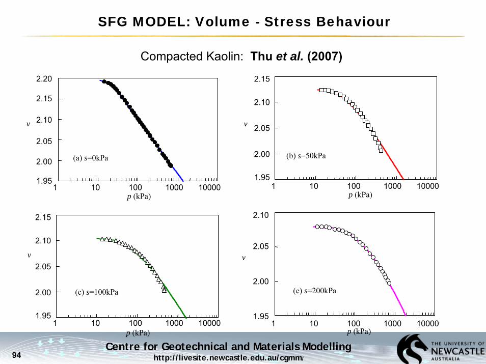
SFG MODEL: Volume - Stress Behaviour
Compacted Kaolin: Thu et al. (2007)
1 10 100 1000 10000
v
2.20
2.15
2.10
2.05
2.00
1.95
p (kPa)
(a) s=0kPa
v
1 10 100 1000 10000
2.15
2.10
2.05
2.00
1.95
p (kPa)
(b) s=50kPa
v
1 10 100 1000 10000
2.15
2.10
2.05
2.00
1.95
p (kPa)
(c) s=100kPa
1 10 100 1000 10000
v
2.10
2.05
2.00
1.95
p (kPa)
(e) s=200kPa

Centre for Geotechnical and Materials Modellinghttp://livesite.newcastle.edu.au/cgmm/95
SFG MODEL: Shear Strength
Shear strength of air-dry sandy soil: Data from Röhm and Vilar (1995).
MeasuredSFG
(d) Suction 400 kPa0
100
200
300
400
500
600
700
0 500 1000 1500
(c) Suction 200 kPa
MeasuredSFG
0
100
200
300
400
500
600
700
0 500 1000 1500
(σ1+σ3) / 2 – ua (kPa)
(σ1−
σ 3) /
2 (k
Pa)
(a) Suction 20 kPa
MeasuredSFG
0
100
200
300
400
500
600
700
0 500 1000 1500
MeasuredSFG
(b) Suction 50 kPa0
100
200
300
400
500
600
700
0 500 1000 1500
(σ1−
σ 3) /
2 (k
Pa)
(σ1+σ3) / 2 – ua (kPa)
(σ1+σ3) / 2 – ua (kPa)
(σ1−
σ 3) /
2 (k
Pa)
(σ1+σ3) / 2 – ua (kPa)
(σ1−
σ 3) /
2 (k
Pa)

Centre for Geotechnical and Materials Modellinghttp://livesite.newcastle.edu.au/cgmm/96
SFG MODEL: Shear Strength
Measured Predicted
0 100 200 300 400 500 6000
50
100
150
200
τ(k
Pa)
s (kPa)
Shear strength of compacted glacial till: Data from Vanapilli (1996).
σn = 200 kPaσn = 100 kPaσn = 25 kPa

Centre for Geotechnical and Materials Modellinghttp://livesite.newcastle.edu.au/cgmm/97
Measured Predicted
(kPa)
(σ1−
σ 3) (k
Pa)
0 50 100 150 200 250 3000
50
100
150
200
250
300
350
400
450
SFG MODEL: Shear Strength
p
Shear strength of compacted kaolin: Data from Wheeler & Sivakuma (2000)
s = 300 kPa
s = 100 kPa
s = 0 kPa

Centre for Geotechnical and Materials Modellinghttp://livesite.newcastle.edu.au/cgmm/98
0
100
200
300
400
500
-100 0 100 200 300 400
SFG MODEL PREDICTION
Example 1: Soil with low air-entry value – yield surface evolution
CA
B D
s
E
B' D'
p
ssa=10 kPa

Centre for Geotechnical and Materials Modellinghttp://livesite.newcastle.edu.au/cgmm/99
SFG MODEL PREDICTION
Example 1: Soil with low air-entry value – volume change
0.40
0.45
0.50
0.55
0.60
0.65
0.70
1 10 100 1000
e
A
B
D
B'
E
NCL, s=0URL, s=0
p

Centre for Geotechnical and Materials Modellinghttp://livesite.newcastle.edu.au/cgmm/100
SFG MODEL PREDICTION
Example 2: Soil with high air-entry value – yield surface evolution
0
500
1000
1500
2000
-1000 -500 0 500 1000 1500 2000
B D
A
s (kPa)
C
sae=500 kPa
kPap

Centre for Geotechnical and Materials Modellinghttp://livesite.newcastle.edu.au/cgmm/101
0.1
0.3
0.5
0.7
0.9
1.1
1 10 100 1000 10000
SFG MODEL PREDICTION
Example 2: Soil with high air-entry value – volume change
p (kPa)
s=0 kPa
s=10 kPa
s=100 kPa
s=500 kPa
s=2000 kPa
e
s=1000 kPa
2.00
1.46
1.01
0.65
0.35
0.11

Centre for Geotechnical and Materials Modellinghttp://livesite.newcastle.edu.au/cgmm/102
-50
0
50
100
150
200
-50 0 50 100 150 200 250 300 350 400
SFG MODEL PREDICTION
Example 3: Compacted soil: yield surface after compaction
p (kPa)
s (kPa)
Elastic zone after compaction
Measured suction levels where collapse starts
A
B E F G H
E' F' G' H'D'
D
Centre for Geotechnical and Materials Modellinghttp://livesite.newcastle.edu.au/cgmm/103
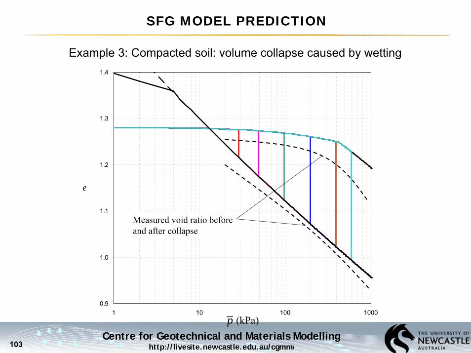
SFG MODEL PREDICTION
Example 3: Compacted soil: volume collapse caused by wetting
D E F
D'
E'
F'
G'
H'I'
NCL (s=0)
AB
e
G HI
0.9
1.0
1.1
1.2
1.3
1.4
1 10 100 1000p (kPa)
Measured void ratio before and after collapse

Centre for Geotechnical and Materials Modellinghttp://livesite.newcastle.edu.au/cgmm/104
5. Hydro-mechanical Coupling: Stress-Strain Relation
Hydro-mechanically coupled model (Sheng, Gens & Sloan, 2004)
( )7 1×
ep ep
r
dddd Ss G
⎛ ⎞ ⎛ ⎞⎛ ⎞= ⎜ ⎟ ⎜ ⎟⎜ ⎟
⎝ ⎠ ⎝ ⎠⎝ ⎠
D W εσR
( )7 1×( )7 7×
ep ep
r
d dd dS sG
⎛ ⎞⎛ ⎞ ⎛ ⎞= ⎜ ⎟⎜ ⎟ ⎜ ⎟
⎝ ⎠⎝ ⎠ ⎝ ⎠
D Wσ εR
Unknown Known
Centre for Geotechnical and Materials Modellinghttp://livesite.newcastle.edu.au/cgmm/105
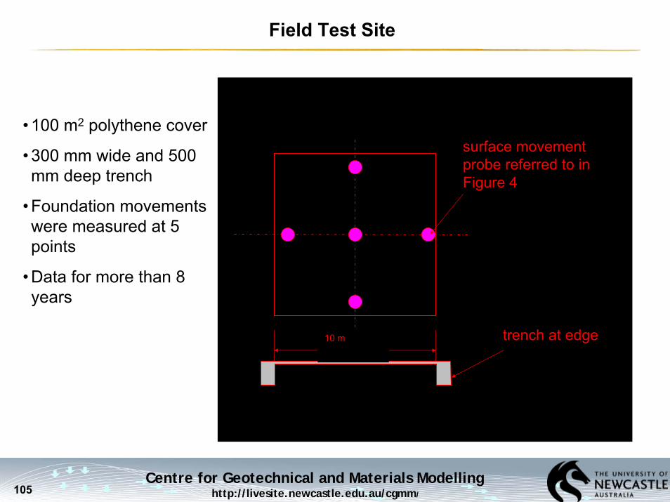
Field Test Site
• 100 m2 polythene cover
• 300 mm wide and 500 mm deep trench
• Foundation movements were measured at 5 points
• Data for more than 8 years
trench at edge10 m
surface movement probe referred to in Figure 4

Centre for Geotechnical and Materials Modellinghttp://livesite.newcastle.edu.au/cgmm/106
Field Test Site
6 m
flexible cover (impermeable)
10 m
constant head (6.0m)
impe
rmea
ble
impe
rmea
ble
wetting/drying boundary

Centre for Geotechnical and Materials Modellinghttp://livesite.newcastle.edu.au/cgmm/107
Field Test Site
0
10
20
30
40
50
0 365 730 1095 1460 1825 2190 2555
Time (days)
Dis
plac
emen
ts (m
m)
measured
FEM prediction (x=0)
Predicted and measured heave under the cover

Centre for Geotechnical and Materials Modellinghttp://livesite.newcastle.edu.au/cgmm/108
-10
0
10
20
30
40
0 365 730 1095 1460 1825 2190 2555
Time (days)
Dis
plac
emen
ts (m
m)
measured
FEM prediction (x=10m)
Predicted and measured heave outside the cover
Field Test Site

Centre for Geotechnical and Materials Modellinghttp://livesite.newcastle.edu.au/cgmm/109
-0.05
0.00
0.05
0.10
0 2 4 6 8 10Distance from the cover centre (m)
Dis
plac
emen
ts (m
) Wet season
Dry season
Mound Shape during Dry and Wet Seasons
Dry → Cover → Cyclic Wetting and Drying