Embed Size (px)
Citation preview

International Journal of Computer Science, Engineering and Applications (IJCSEA) Vol.5, No.4/5, October 2015
DOI : 10.5121/ijcsea.2015.5501 1
CHARACTERISTIC SPECIFIC PRIORITIZED DYNAMIC
AVERAGE BURST ROUND ROBIN SCHEDULING FOR
UNIPROCESSOR AND MULTIPROCESSOR
ENVIRONMENT
Amar Ranjan Dash1, Sandipta Kumar Sahu
2, Sanjay Kumar Samantra
2 and
Sradhanjali Sabat2
1Department of Computer Science, Berhampur University, Berhampur, India
2Department of Computer Science, NIST, Berhampur, India
ABSTRACT
CPU scheduling is one of the most crucial operations performed by operating systems. Different
conventional algorithms like FCFS, SJF, Priority, and RR (Round Robin) are available for CPU
Scheduling. The effectiveness of Priority and Round Robin scheduling algorithm completely depends on
selection of priority features of processes and on the choice of time quantum. In this paper a new CPU
scheduling algorithm has been proposed, named as CSPDABRR (Characteristic specific Prioritized
Dynamic Average Burst Round Robin), that uses seven priority features for calculating priority of
processes and uses dynamic time quantum instead of static time quantum used in RR. The performance of
the proposed algorithm is experimentally compared with traditional RR and Priority scheduling algorithm
in both uni-processor and multi-processor environment. The results of our approach presented in this
paper demonstrate improved performance in terms of average waiting time, average turnaround time, and
optimal priority feature.
KEYWORDS
CPU Scheduling, Round Robin, Dynamic Time Quantum, Priority, Multi-Processor Environment.
1. INTRODUCTION
Operating systems are resource managers. The resources managed by Operating systems are
hardware, storage units, input devices, output devices and data. Process scheduling is one of the
functions performed by Operating systems. CPU scheduling is the method of selecting a process
from the ready queue and allocating the CPU to it. Whenever CPU becomes idle, a waiting
process from ready queue is selected and CPU is allocated to that. The performance of the
scheduling algorithm mainly depends on CPU utilization, throughput, turnaround time, waiting
time, response time, and context switch.
Conventionally four CPU scheduling techniques were there viz. FCFS, SJF, Priority, and RR. In
FCFS, the process that requests the CPU first is allocated to the CPU first. In SJF, the CPU is
allocated to the process with smallest burst time. In priority scheduling algorithm a priority is
associated with each process, and the CPU is allocated to the process with the highest priority. In
RR a small unit of time is used which is called Time Quantum or Time slice. The CPU scheduler
goes around the Ready Queue allocating the CPU to each process for a time interval up to 1 time

International Journal of Computer Science, Engineering and Applications (IJCSEA) Vol.5, No.4/5, October 2015
2
quantum. If a process’s CPU burst exceeds 1 time quantum, that process is pre-empted and is put
back in the ready queue.
Different CPU scheduling algorithms described by Abraham Silberschatz et al. [1], viz. FCFS
(First Come First Served), SJF (Shortest Job First), Priority and RR (Round Robin). Neetu Goel
et al. [2] make a comparative analysis of CPU scheduling algorithms with the concept of
schedulers. Jayashree S. Somani et al. [3] also make a similar analysis but with their
characteristics and applications.
Figure 1: State Transition diagram of processes with different queues and schedulers.
Turnaround time is the time interval from the submission time of a process to the completion time
of a process. Waiting time is the sum of periods spent waiting in the ready queue. The time from
the submission of a process until the first response is called Response time. The CPU utilization is
the percentage of time CPU remains busy. The number of processes completed per unit time is
called Throughput. Context switch is the process of swap-out the pre-executed process from CPU
and swap-in a new process to CPU. A scheduling algorithm can be optimized by minimizing
response time, waiting time and turnaround time and by maximizing CPU utilization, throughput.
Recently researchers try to improve the performance of Round Robin scheduling algorithm by
manipulating the time slice. Rami J. Matarneh [4] designed an algorithm Self Adjustment Round
Robin (SARR), in which after each cycle the median of burst time of the processes is calculated
and used as time quantum. Abbas Noon et al. [5] develop an algorithm in which they calculate
mean of burst time of all processes to use as time quantum. H.S.Behera et al. [6] also presents
similar type of algorithm, but they rearrange the process during the next execution. It selects the

International Journal of Computer Science, Engineering and Applications (IJCSEA) Vol.5, No.4/5, October 2015
3
process with lowest burst time, then process with highest burst time, then process with second
lowest burst time, and so on.
Besides manipulating the time-slice some researchers combine the SJF and RR to improve the
performance of RR scheduling algorithm. Among them Ajit Singh et al. [7] develop a scheduling
algorithm in which in the first round they take a dynamic time quantum and then double the time
quantum after every cycle. Manish Kumar Mishra et al. [8] developed a scheduling algorithm,
which chooses the burst time of shortest process as new time quantum after each cycle. Rishi
Verma [9] calculates the time quantum after every cycle by subtracting the minimum burst time
from maximum burst time. Radhe Shyam et al. [10] also developed a scheduling algorithm in
which they calculate the time quantum after every cycle by taking the square root of the
multiplication of mean and the highest burst time. Amar Ranjan Dash et al. [11] developed an
algorithm by arranging the processes in ascending order of burst time and by taking the average
burst-time of the processes as time-slice to improve the performance of conventional Round
Robin.
Bashir Alam et al. [12] develop Fuzzy Priority CPU Scheduling (FPCS) algorithm. They generate
a fuzzy inference engine which gives a dynamic priority based on given static priority, Remaining
Burst Time, and waiting time. H. S. Behera et al. [13] develop an Improved Fuzzy Based CPU
Scheduling (IFCS) algorithm. They first calculate fuzzy membership value of priority (µp), burst
time (µb), response ration (µh) of individual processes, and then arrange the processes according
to their membership value, which is the maximum value among µp, µb, µh.
M. Ramakrishna et al. [14] and Ishwari Singh Rajput et al. [15] integrate the concept of priority
scheduling with RR scheduling to optimize the Round Robin scheduling. They only consider
shortness of the processes as priority component. H.S.Behera et al. in [16] also develop the same
type of algorithm but they use the weighted mean of processes (TQwm) and the root mean square
(TQrms). If the burst time of processes is less than the average burst time, then use TQwm as Time
Quantum. Otherwise use the addition of TQwm and TQrms as the Time Quantum. H.S.Behera et al.
[17, 18] develop a prioritized round robin where they take shortness of the process and the
number of context switch as priority component. They take a random time slice as original time
slice. They add the priority components with original time slice and then calculate an intelligent
time slice from that after each cycle. Zena Hussain Khalil et al. [19] modified the algorithm in
[17] by adding the concept of Response ration into it.
H.S.Behera et al. [20] develop a round robin algorithm for two processor based real time system.
They consider that one processor deal with CPU intensive process and another processor deal
with I/O intensive process. They consider Gantt chart for each. But they don’t include the priority
component of processes in the algorithm. Previously researchers work on different scheduling
algorithms, but in Uniprocessor environment. In this paper we work on a prioritized round robin
technique for both uniprocessor and multiprocessor environment.
The rest of the paper is organized as follows: Section 2 presents a comparative analysis of
conventional scheduling algorithm. Section 3 presents the proposed algorithm. In section 4, we
make a comparative analysis of round robin, priority and our proposed algorithm experimentally
with six test cases both in uniprocessor and multiprocessor environment. In section 5 we analyze
the results obtained from our analysis. Section 6 provides the concluding remarks.
2. CONVENTIONAL SCHEDULING ALGORITHMS
Four conventional CPU scheduling algorithms are there FCFS, SJF, RR and Priority. FCFS
scheduling algorithm arranges the process as per their arrival time. If more than one process
International Journal of Computer Science, Engineering and Applications (IJCSEA) Vol.5, No.4/5, October 2015
4
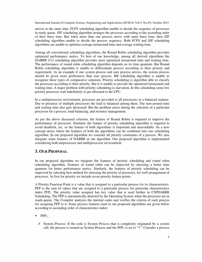
arrives at the same time, FCFS scheduling algorithm unable to decide the sequence of processes
in ready queue. SJF scheduling algorithm arranges the processes according to the ascending order
of their burst time. But when more than one process arrive with same burst time, then SJF
scheduling algorithm unable to decide the process sequence. Both FCFS and SJF scheduling
algorithms are unable to optimize average turnaround time and average waiting time.
Among all conventional scheduling algorithms, the Round Robin scheduling algorithm provides
optimized performance metics. To best of our knowledge, among all derived algorithms the
DABRR [11] scheduling algorithm provides most optimized turnaround time and waiting time.
The performance of round robin scheduling algorithm depends on its time quantum. But Round
Robin scheduling algorithm is unable to differentiate process according to their priority and
requirement. As an example if one system process and user process arrives, the system process
should be given more preferences than user process. RR scheduling algorithm is unable to
recognize these types of comparative solutions. Priority scheduling is algorithm able to classify
the processes according to their priority. But it is unable to provide the optimized turnaround and
waiting time. A major problem with priority scheduling is starvation. In this scheduling some low
priority processes wait indefinitely to get allocated to the CPU.
In a multiprocessor environment, processes are provided to all processors in a balanced manner.
Due to presence of multiple processors the load is balanced among them. The turn-around time
and waiting time also gets decreased. But the problem arises during the selection of a particular
processor for a process, load balancing, and resource management.
As per the above discussed criterion, the feature of Round Robin is required to improve the
performance of processor. Similarly the feature of priority scheduling algorithm is required to
avoid deadlock, etc. so the feature of both algorithms is important and unavoidable. So a new
concept arises where the features of both the algorithms can be combined into one scheduling
algorithm. In our proposed algorithm we consider all priority constraints of a process. We also
integrate some features of DABRR in our algorithm. Our proposed algorithm is implemented
considering both uniprocessor and multiprocessor environment.
3. OUR PROPOSAL
In our proposed algorithm we integrate the features of priority scheduling and round robin
scheduling algorithm. Features of round robin can be improved by choosing a better time
quantum for better performance metics. Similarly, the features of priority scheduling can be
improved by selecting best method for choosing the priority of processes, for well arrangement of
processes. At first for priority we include seven priority feature points.
A Priority Function Point is a value that is assigned to a particular process for its characteristics.
PFP is the sum of values that are assigned to a particular process for particular characteristics
index PFPi. The priority value assigned has key value that is used further in CSPDABRR
Scheduling .The PFP is automatically detected by the Operating System when the processes are in
ready-queue. The Compiler analyzes the internal codes and verifies the criteria of each process
for assigning PFP to it. Some process features used in our proposed algorithms are given below
according to ascending order of characteristics index:
� PFP1:
� System Process: If the code is System Process that is completely originated by a system
call, the process is termed as System Process and the PFP1 is set to “1”. Consider a process

International Journal of Computer Science, Engineering and Applications (IJCSEA) Vol.5, No.4/5, October 2015
5
“Services.exe” in windows Operating System which is completely System oriented process
which runs automatically with the start of Operating System.
� User Process: If the process contains Kernel Calls rapidly but originated by User function
calls then the process is termed as User Process and the PFP1 is set to 2. Consider a process
“Explorer.exe” in windows Operating System which is incited by login users which
completely operates with system calls.
� PFP2:
Types of process interrupts: Every Electronic System supports interrupts for support of multi
tasking and acceptance of hardware interrupts to reliability and efficiency we can categorize the
processes into two parts as follows
� Processes with hardware interrupts: Hardware interrupts are the interrupts that have been
called directly by hardware units for I/O read, Memory Read, I/O write, Memory write the
processes with max no. of any hardware command are considered as hardware interrupts.
These processes has a high PFP2 value as compared to software interrupts and the value is
set to “3”.consider a function “EvtInterruptIsr” for event handling in window operating
system.
� Processes with software interrupts: Processes with software interrupt can be calculated by
compile time. So they can be considered as criteria as they take a major part in program
execution. If the no of software interrupt is count to be more than that of I/O calls in
process then they are categorized under software interrupt list. The PFP2 value is set to
“2”.In windows Operating system some software interrupts are CLI (Clear Interrupts), STI
(SetInterrupts) and POPF (PopFlags).
� Process without any interrupts: the PFP2 value of processes without interrupts is set to “1”.
Like “Garbage collector” process runs periodically without any interrupt.
� PFP3:
Execution Time Of task: Every process consists of codes and the execution time of the process
can be calculated easily by compile time. Depending on bites of instruction, no of clock cycle and
instruction length of processes can easily provide the information of execution time of process. If
we consider the execution time of any tasks for determination of PFP3 values we can classify
tasks into three basic categories as follows:
� Anonymous Execution time: While compile time, if the process has very found that the
instruction has not any time bound from its originating time then the task is categorized
under Anonymous Execution time process and has a very High PFP3 value and set to “3”.
NTLDR loader process in windows Operating System for booting.
� Medium calculable Execution time: While compile time, if any process execution time is
calculated but can be extended due to specific regions then they are categorized under
Medium calculable Execution time and the PFP3 value is set to “2”.WMIC.exe for
information collection for data transfer.
� Real time Execution time: While compile time, if any process execution time is found
dedicated to the process by the process originating function then the processes is
categorized under Real time Execution time and the PFP3 value is set to “1”.Consider a
function ‘DWORD WINAPI SleepEx(_In_ DWORD dwMilliseconds,_In_ BOOL
bAlertable);‘responsible for sleep while battery is critically low.
International Journal of Computer Science, Engineering and Applications (IJCSEA) Vol.5, No.4/5, October 2015
6
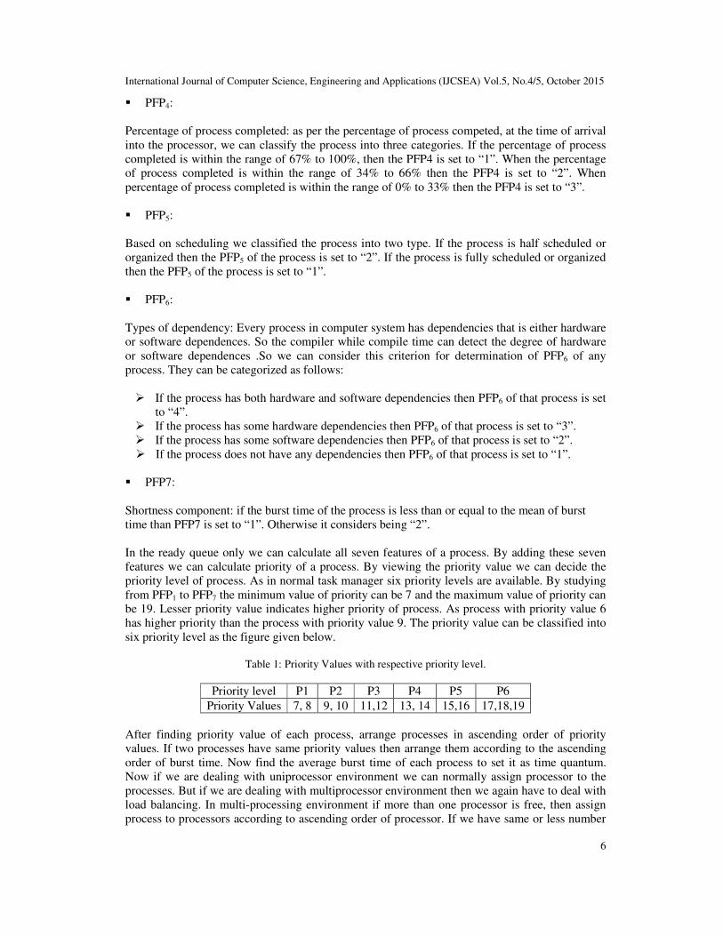
� PFP4:
Percentage of process completed: as per the percentage of process competed, at the time of arrival
into the processor, we can classify the process into three categories. If the percentage of process
completed is within the range of 67% to 100%, then the PFP4 is set to “1”. When the percentage
of process completed is within the range of 34% to 66% then the PFP4 is set to “2”. When
percentage of process completed is within the range of 0% to 33% then the PFP4 is set to “3”.
� PFP5:
Based on scheduling we classified the process into two type. If the process is half scheduled or
organized then the PFP5 of the process is set to “2”. If the process is fully scheduled or organized
then the PFP5 of the process is set to “1”.
� PFP6:
Types of dependency: Every process in computer system has dependencies that is either hardware
or software dependences. So the compiler while compile time can detect the degree of hardware
or software dependences .So we can consider this criterion for determination of PFP6 of any
process. They can be categorized as follows:
� If the process has both hardware and software dependencies then PFP6 of that process is set
to “4”.
� If the process has some hardware dependencies then PFP6 of that process is set to “3”.
� If the process has some software dependencies then PFP6 of that process is set to “2”.
� If the process does not have any dependencies then PFP6 of that process is set to “1”.
� PFP7:
Shortness component: if the burst time of the process is less than or equal to the mean of burst
time than PFP7 is set to “1”. Otherwise it considers being “2”.
In the ready queue only we can calculate all seven features of a process. By adding these seven
features we can calculate priority of a process. By viewing the priority value we can decide the
priority level of process. As in normal task manager six priority levels are available. By studying
from PFP1 to PFP7 the minimum value of priority can be 7 and the maximum value of priority can
be 19. Lesser priority value indicates higher priority of process. As process with priority value 6
has higher priority than the process with priority value 9. The priority value can be classified into
six priority level as the figure given below.
Table 1: Priority Values with respective priority level.
Priority level P1 P2 P3 P4 P5 P6
Priority Values 7, 8 9, 10 11,12 13, 14 15,16 17,18,19
After finding priority value of each process, arrange processes in ascending order of priority
values. If two processes have same priority values then arrange them according to the ascending
order of burst time. Now find the average burst time of each process to set it as time quantum.
Now if we are dealing with uniprocessor environment we can normally assign processor to the
processes. But if we are dealing with multiprocessor environment then we again have to deal with
load balancing. In multi-processing environment if more than one processor is free, then assign
process to processors according to ascending order of processor. If we have same or less number

International Journal of Computer Science, Engineering and Applications (IJCSEA) Vol.5, No.4/5, October 2015
7
of processes than the number of processor, then don’t change process-processor bonding to stop
unnecessary transfer of resources and information of one process from one processor to another.
3.1. CSPDABRR Algorithm
TQ : Time Quantum
RQ : Ready Queue
PQ : Priority Queue
TBT : Total Burst Time
Pi : Process at ith index
PFPj : jth Priority Feature Point
n : number of process in Ready Queue
i : used as index of ready queue or priority queue
m : number of processor in multi processing environment
FLOOR: Mathematical function to found the largest number smaller than given float
Figure 2: CSPDABRR scheduling algorithm
International Journal of Computer Science, Engineering and Applications (IJCSEA) Vol.5, No.4/5, October 2015
8
3.2. Assumption
During analysis we have considered pre-emptive only. In each test case 5 processes are analyzed
in both uniprocessor & multiprocessor environment. Corresponding burst time and arrival time of
processes are known before execution. The context switch time of processes has been considered
as zero. The time required for arranging the processes in ascending order of priority also
considered as zero. We assume the static time quantum for round robin as 25.
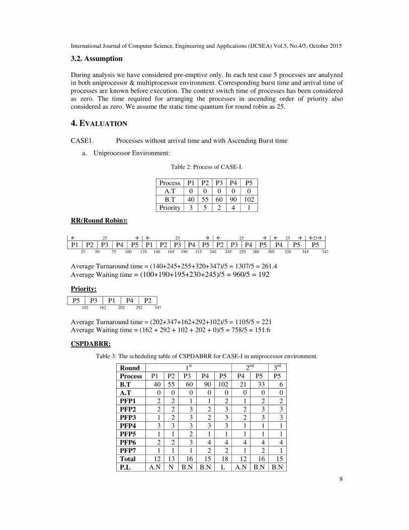
4. EVALUATION CASE1. Processes without arrival time and with Ascending Burst time
a. Uniprocessor Environment:
Table 2: Process of CASE-I.
Process P1 P2 P3 P4 P5
A.T 0 0 0 0 0
B.T 40 55 60 90 102
Priority 3 5 2 4 1
RR(Round Robin):
� 25 � � 25 � � 25 � � 25 � �25�
P1 P2 P3 P4 P5 P1 P2 P3 P4 P5 P2 P3 P4 P5 P4 P5 P5 25 50 75 100 125 140 165 190 215 240 245 255 280 305 320 345 347
Average Turnaround time = (140+245+255+320+347)/5 = 1307/5 = 261.4
Average Waiting time = (100+190+195+230+245)/5 = 960/5 = 192
Priority:
P5 P3 P1 P4 P2 102 162 202 292 347
Average Turnaround time = (202+347+162+292+102)/5 = 1105/5 = 221
Average Waiting time = (162 + 292 + 102 + 202 + 0)/5 = 758/5 = 151.6
CSPDABRR:
Table 3: The scheduling table of CSPDABRR for CASE-I in uniprocessor environment.
Round 1st 2
nd 3
rd
Process P1 P2 P3 P4 P5 P4 P5 P5
B.T 40 55 60 90 102 21 33 6
A.T 0 0 0 0 0 0 0 0
PFP1 2 2 1 1 2 1 2 2
PFP2 2 2 3 2 3 2 3 3
PFP3 1 2 3 2 3 2 3 3
PFP4 3 3 3 3 3 1 1 1
PFP5 1 1 2 1 1 1 1 1
PFP6 2 2 3 4 4 4 4 4
PFP7 1 1 1 2 2 1 2 1
Total 12 13 16 15 18 12 16 15
P.L A.N N B.N B.N L A.N B.N B.N
International Journal of Computer Science, Engineering and Applications (IJCSEA) Vol.5, No.4/5, October 2015
9
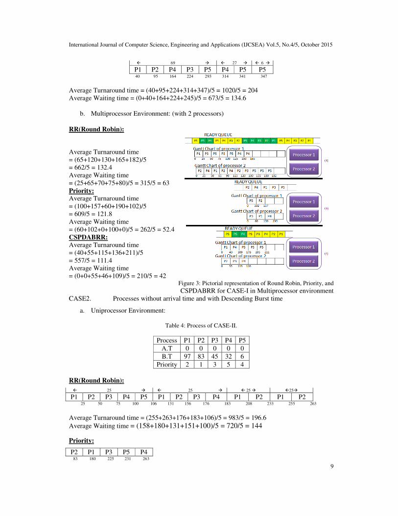
� 69 � � 27 � � 6 �
P1 P2 P4 P3 P5 P4 P5 P5 40 95 164 224 293 314 341 347
Average Turnaround time = (40+95+224+314+347)/5 = 1020/5 = 204
Average Waiting time = (0+40+164+224+245)/5 = 673/5 = 134.6
b. Multiprocessor Environment: (with 2 processors)
RR(Round Robin):
Average Turnaround time
= (65+120+130+165+182)/5
= 662/5 = 132.4
Average Waiting time
= (25+65+70+75+80)/5 = 315/5 = 63
Priority: Average Turnaround time
= (100+157+60+190+102)/5
= 609/5 = 121.8
Average Waiting time
= (60+102+0+100+0)/5 = 262/5 = 52.4
CSPDABRR:
Average Turnaround time
= (40+55+115+136+211)/5
= 557/5 = 111.4
Average Waiting time
= (0+0+55+46+109)/5 = 210/5 = 42 Figure 3: Pictorial representation of Round Robin, Priority, and
CSPDABRR for CASE-I in Multiprocessor environment
CASE2. Processes without arrival time and with Descending Burst time
a. Uniprocessor Environment:
Table 4: Process of CASE-II.
Process P1 P2 P3 P4 P5
A.T 0 0 0 0 0
B.T 97 83 45 32 6
Priority 2 1 3 5 4
RR(Round Robin):
� 25 � � 25 � � 25 � �25�
P1 P2 P3 P4 P5 P1 P2 P3 P4 P1 P2 P1 P2 25 50 75 100 106 131 156 176 183 208 233 255 263
Average Turnaround time = (255+263+176+183+106)/5 = 983/5 = 196.6
Average Waiting time = (158+180+131+151+100)/5 = 720/5 = 144
Priority:
P2 P1 P3 P5 P4 83 180 225 231 263
International Journal of Computer Science, Engineering and Applications (IJCSEA) Vol.5, No.4/5, October 2015
10
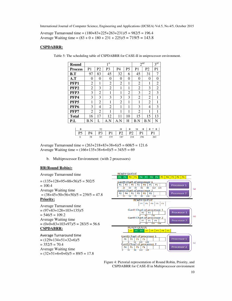
Average Turnaround time = (180+83+225+263+231)/5 = 982/5 = 196.4
Average Waiting time = (83 + 0 + 180 + 231 + 225)/5 = 719/5 = 143.8
CSPDABRR:
Table 5: The scheduling table of CSPDABRR for CASE-II in uniprocessor environment.
Round 1st 2nd 3rd
Process P1 P2 P3 P4 P5 P1 P2 P1
B.T 97 83 45 32 6 45 31 7
A.T 0 0 0 0 0 0 0 0
PFP1 2 1 2 2 1 2 1 2
PFP2 2 3 2 1 1 2 3 2
PFP3 3 2 1 1 2 3 2 3
PFP4 3 3 3 3 3 2 2 1
PFP5 1 2 1 2 1 1 2 1
PFP6 3 4 2 1 1 3 4 3
PFP7 2 2 1 1 1 2 1 1
Total 16 17 12 11 10 15 15 13
P.L B.N L A.N A.N H B.N B.N N
� 52 � � 38 � � 7 �
P5 P4 P3 P1 P2 P2 P1 P1 6 38 83 135 187 218 256 263
Average Turnaround time = (263+218+83+38+6)/5 = 608/5 = 121.6
Average Waiting time = (166+135+38+6+0)/5 = 345/5 = 69
b. Multiprocessor Environment: (with 2 processors)
RR(Round Robin):
Average Turnaround time
= (135+128+95+88+56)/5 = 502/5
= 100.4
Average Waiting time
= (38+45+50+56+50)/5 = 239/5 = 47.8
Priority:
Average Turnaround time
= (97+83+128+103+135)/5
= 546/5 = 109.2
Average Waiting time
= (0+0+83+103+97)/5 = 283/5 = 56.6
CSPDABRR:
Average Turnaround time
= (129+134+51+32+6)/5
= 352/5 = 70.4
Average Waiting time
= (32+51+6+0+0)/5 = 89/5 = 17.8
Figure 4: Pictorial representation of Round Robin, Priority, and
CSPDABRR for CASE-II in Multiprocessor environment

International Journal of Computer Science, Engineering and Applications (IJCSEA) Vol.5, No.4/5, October 2015
11
CASE3. Processes without arrival time and with random Burst time
a. Uniprocessor Environment:
Table 6: Process of CASE-III.
Process P1 P2 P3 P4 P5
A.T 0 0 0 0 0
B.T 12 32 6 54 83
Priority 2 1 4 3 5
RR(Round Robin):
� 25 � � 25 � � 25 � �25�
P1 P2 P3 P4 P5 P2 P4 P5 P4 P5 P5 12 37 43 68 93 100 125 150 154 179 187
Average Turnaround time = (12+100+43+154+187)/5 = 496/5 = 99.2
Average Waiting time = (0+68+37+104+104)/5 = 313/5 = 62.6
Priority:
P2 P1 P4 P3 P5 32 44 98 104 187
Average Turnaround time = (32+44+104+98+187)/5 = 465/5 = 93
Average Waiting time = (32 + 0 + 98 + 44 + 104)/5 = 278/5 = 55.6
CSPDABRR: Table 7: The scheduling table of CSPDABRR for CASE-III in uniprocessor environment.
Round 1st 2
nd 3
rd
Process P1 P2 P3 P4 P5 P4 P5 P5
B.T 12 32 6 54 83 17 46 15
A.T 0 0 0 0 0 0 0 0
PFP1 1 2 1 1 2 1 2 2
PFP2 1 2 2 3 2 3 2 2
PFP3 2 3 1 2 3 2 3 3
PFP4 3 3 3 3 3 1 2 1
PFP5 1 2 1 2 2 2 2 2
PFP6 1 2 2 3 4 3 4 4
PFP7 1 1 1 2 2 1 2 1
Total 10 15 11 16 18 13 17 15
P.L H B.N A.N B.N L N L B.N
� 37 � � 31 � � 15 �
P1 P3 P4 P2 P5 P4 P5 P5 12 18 55 87 124 141 172 187
Average Turnaround time = (12+87+18+141+187)/5 = 445/5 = 89
Average Waiting time = (0+55+12+87+104)/5 = 258/5 = 51.6
b. Multiprocessor Environment: (with 2 processors)
RR(Round Robin):
Average Turnaround time
International Journal of Computer Science, Engineering and Applications (IJCSEA) Vol.5, No.4/5, October 2015
12
= (12+50+18+79+108)/5
= 267/5 = 53.4
Average Waiting time
= (0+18+12+25+25)/5 = 80/5 = 16
Priority:
Average Turnaround time
= (12+32+38+66+121)/5
= 269/5 = 53.8
Average Waiting time
= (0+0+32+12+38)/5 = 82/5 = 16.4
CSPDABRR:
Average Turnaround time
= (12+44+6+61+126)/5
= 249/5 = 49.5
Average Waiting time
= (0+12+0+7+43)/5 = 62/5 = 12.4
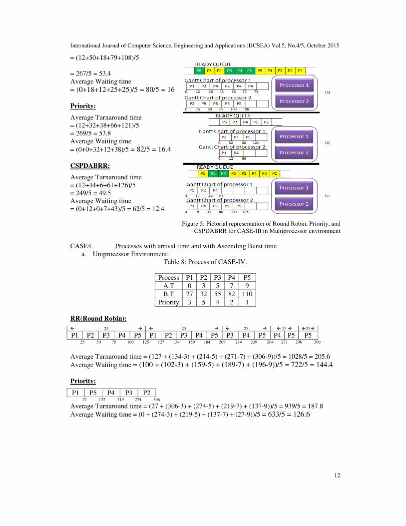
Figure 5: Pictorial representation of Round Robin, Priority, and
CSPDABRR for CASE-III in Multiprocessor environment
CASE4. Processes with arrival time and with Ascending Burst time
a. Uniprocessor Environment:
Table 8: Process of CASE-IV.
Process P1 P2 P3 P4 P5
A.T 0 3 5 7 9
B.T 27 32 55 82 110
Priority 3 5 4 2 1
RR(Round Robin):
� 25 � � 25 � � 25 � � 25 � �25�
P1 P2 P3 P4 P5 P1 P2 P3 P4 P5 P3 P4 P5 P4 P5 P5 25 50 75 100 125 127 134 159 184 209 214 239 264 271 296 306
Average Turnaround time = (127 + (134-3) + (214-5) + (271-7) + (306-9))/5 = 1028/5 = 205.6
Average Waiting time = (100 + (102-3) + (159-5) + (189-7) + (196-9))/5 = 722/5 = 144.4
Priority:
P1 P5 P4 P3 P2 27 137 219 274 306
Average Turnaround time = (27 + (306-3) + (274-5) + (219-7) + (137-9))/5 = 939/5 = 187.8
Average Waiting time = (0 + (274-3) + (219-5) + (137-7) + (27-9))/5 = 633/5 = 126.6
International Journal of Computer Science, Engineering and Applications (IJCSEA) Vol.5, No.4/5, October 2015
13
CSPDABRR:
Table 9: The scheduling table of CSPDABRR for CASE-IV in uniprocessor environment.
Round 1st 2
nd 3
rd 4
th
Process P1 P2 P3 P4 P5 P4 P5 P5
B.T 27 32 55 82 110 13 41 14
A.T 0 3 5 7 9 7 9 9
PFP1 1 2 2 1 1 1 1 1
PFP2 3 2 3 2 3 2 3 3
PFP3 3 3 2 3 1 3 1 1
PFP4 3 3 3 3 3 1 2 1
PFP5 1 1 2 2 1 2 1 1
PFP6 4 2 3 4 4 4 4 4
PFP7 1 1 1 2 2 1 2 1
Total 16 14 16 17 15 14 14 12
P.L B.N N B.N L B.N N N A.N
�27� � 69 � � 27 � �14 �
P1 P2 P5 P3 P4 P4 P5 P5 27 59 128 183 252 265 292 306
Average Turnaround time = (27 + (59-3) + (183-5) + (265-7) + (306-9))/5 = 816/5 = 163.2
Average Waiting time = (0 + (27 – 3) + (128 - 5) + (183 - 7) + (196 - 9))/5 = 510/5 = 102
b. Multiprocessor Environment: (with 2 processors)
RR(Round Robin):
Average Turnaround time = (55 + (62-3) + (105-5) + (137-7) + (172-9))/5 = 507/5 = 101.4
Average Waiting time = (28 + (30 - 3) + (50 - 5) + (55 - 7) + (62-9))/5 = 201/5 = 40.2
Priority:
Average Turnaround time = (27 + (35-3) + (172-5) + (117-7) + (137-9))/5 = 464/5 = 92.8
Average Waiting time = (0 + (3-3) + (117-5) + (35-7) + (27-9))/5 = 158/5 = 31.6
CSPDABRR: Table 10: The scheduling table of CSPDABRR for
CASE-IV in multiprocessor environment.
Round 1st 2
nd 3
rd 4
th
Process P1 P2 P3 P4 P5 P5
B.T 27 32 55 82 110 28
A.T 0 3 5 7 9 9
PFP1 1 2 2 1 1 1
PFP2 3 2 3 2 3 3
PFP3 3 3 2 3 1 1
PFP4 3 3 3 3 3 1
PFP5 1 1 2 2 1 1
PFP6 4 2 3 4 4 4
PFP7 1 1 1 1 2 1
Total 16 14 16 16 15 12
P.L B.N N B.N B.N B.N A.N
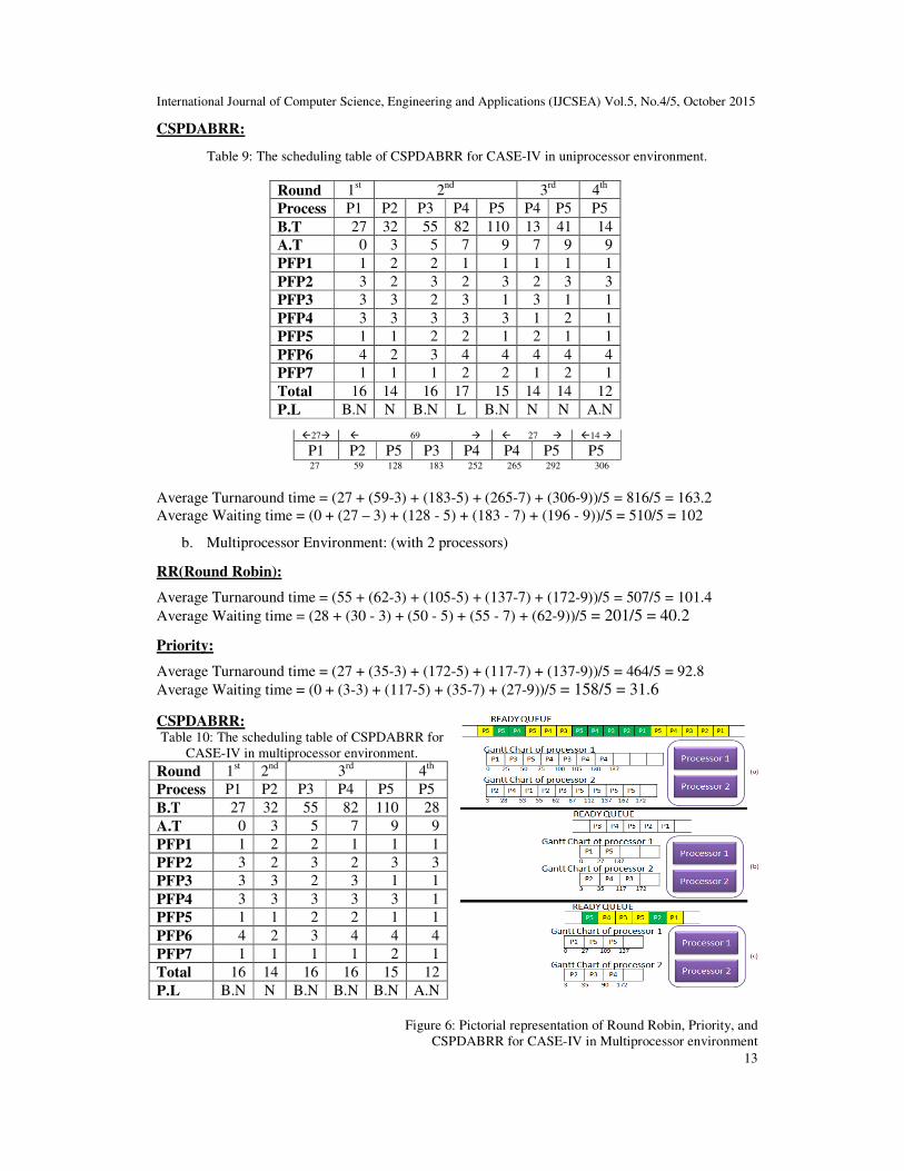
Figure 6: Pictorial representation of Round Robin, Priority, and
CSPDABRR for CASE-IV in Multiprocessor environment

International Journal of Computer Science, Engineering and Applications (IJCSEA) Vol.5, No.4/5, October 2015
14
Average Turnaround time = (27 + (35-3) + (90-5) + (172-7) +(137-9))/5 = 437/5 = 87.4
Average Waiting time = (0 + (3-3) + (35-5) + (90-7) + (27-9))/5 = 131/5 = 26.2
CASE5. Processes with arrival time and with Descending Burst time
a. Uniprocessor Environment:
Table 11: Process of CASE-V.
Process P1 P2 P3 P4 P5
A.T 0 2 4 8 16
B.T 105 80 60 45 32
Priority 2 3 4 5 1
RR(Round Robin):
� 25 � � 25 � � 25 � � 25 � � 25�
P1 P2 P3 P4 P5 P1 P2 P3 P4 P5 P1 P2 P3 P1 P2 P1 25 50 75 100 125 150 175 200 220 227 252 277 287 312 317 322
Average Turnaround time = (322 + (317-2) + (287-4) + (220-8) + (227-16))/5 = 1343/5 = 268.6
Average Waiting time = (217 + (237-2) + (227-4) + (175-8) + (195-16))/5 = 1021/5 = 204.2
Priority:
P1 P5 P2 P3 P4 105 137 217 277 322
Average Turnaround time = (105 + (217-2) + (277-4) + (322-8) + (137-16))/5 = 1028/5 = 205.6
Average Waiting time = (0 + (137-2) + (217-4) + (277-8) + (105-16))/5 = 706/5 = 141.2
CSPDABRR:
Table 12: The scheduling table of CSPDABRR for CASE-V in uniprocessor environment.
Round 1st 2nd 3rd 4th
Process P1 P2 P3 P4 P5 P2 P3 P2
B.T 105 80 60 45 32 26 6 10
A.T 0 2 4 8 16 2 4 2
PFP1 2 1 2 1 1 1 2 1
PFP2 2 2 3 3 2 2 3 2
PFP3 2 1 2 1 2 1 2 1
PFP4 3 3 3 3 3 1 1 1
PFP5 1 2 1 1 1 2 1 2
PFP6 4 4 4 3 2 4 4 4
PFP7 1 2 2 1 1 2 1 1
Total 15 15 17 13 12 13 14 12
P.L B.N B.N L N A.N N N A.N
�105� � 54 � � 16 � � 10 �
P1 P5 P4 P2 P3 P2 P3 P2 105 137 182 236 290 306 312 322
Average Turnaround time = (105 + (322-2) + (312-4) + (182-8) + (137-16))/5 = 1028/5 = 205.6
Average Waiting time = (0 + (242-2) + (252-4) + (137-8) + (105-16))/5 = 706/5 = 141.2

International Journal of Computer Science, Engineering and Applications (IJCSEA) Vol.5, No.4/5, October 2015
15
b. Multiprocessor Environment: (with 2 processors)
RR(Round Robin): Average Turnaround time = (174 + (150-2) + (144-4) + (120-8) + (109-16))/5 = 667/5 = 133.4
Average Waiting time = (69 + (70-2) + (84-4) + (75-8) + (77-16))/5 = 345/5 = 69
Priority:
Average Turnaround time = (105 + (82-2) + (165-4) + (159-8) + (114-16))/5 = 595/5 = 119
Average Waiting time = (0 + (2 - 2) + (105 - 4) + (114 - 8) + (82 - 16))/5 = 273/5 = 54.6
CSPDABRR:
Table 13: The scheduling table of CSPDABRR for
CASE-V in multiprocessor environment.
Round 1st 2
nd 3
rd 4
th
Process P1 P2 P3 P4 P5 P3
B.T 105 80 60 45 32 15
A.T 0 2 4 8 16 4
PFP1 2 1 2 1 1 2
PFP2 2 2 3 3 2 3
PFP3 2 1 2 1 2 2
PFP4 3 3 3 3 3 1
PFP5 1 2 1 1 1 1
PFP6 4 4 4 3 2 4
PFP7 1 1 2 1 1 1
Total 15 14 17 13 12 14
P.L B.N N L N AN N Figure 7: Pictorial representation of Round Robin, Priority, and
CSPDABRR for CASE-V in Multiprocessor environment
Average Turnaround time = (105 + (82-2) + (174-4) + (150-8) + (114-16)/5 = 595/5 = 119
Average Waiting time = (0 + (2-2) + (114-4) + (105-8) + (82-16))/5 = 273/5 = 54.6
CASE6. Processes with arrival time and with Random Burst time
a. Uniprocessor Environment:
Table 14: Process of CASE-VI.
Process P1 P2 P3 P4 P5
A.T 0 5 8 15 20
B.T 45 90 70 38 55
Priority 5 1 3 4 2
RR(Round Robin):
� 25 � � 25 � � 25 � � 25�
P1 P2 P3 P4 P5 P1 P2 P3 P4 P5 P2 P3 P5 P2 25 50 75 100 125 145 170 195 208 233 258 278 283 298
Average Turnaround time = (145+ (298-5) + (278-8) + (208-15) + (283-20))/5 = 1164/5 = 232.8
Average Waiting time = (100 + (208-5) + (208-8) + (170-15) + (228-20))/5 = 866/5 = 173.2

International Journal of Computer Science, Engineering and Applications (IJCSEA) Vol.5, No.4/5, October 2015
16
Priority:
P1 P2 P5 P3 P4 45 135 190 260 298
Average Turnaround time = (45 + (135-5) + (260-8) + (298-15) + (190-20))/5 = 880/5 = 176
Average Waiting time = (0 + (45-5) + (190-8) + (260-15) + (135-20))/5 = 582/5 = 116.4
CSPDABRR:
Table 15: The scheduling table of CSPDABRR for CASE-VI in uniprocessor environment.
Round 1st 2nd 3rd 4th
Process P1 P2 P3 P4 P5 P2 P3 P2
B.T 45 90 70 38 55 27 7 10
A.T 0 5 8 15 20 5 8 5
PFP1 1 2 2 1 1 2 2 2
PFP2 2 3 2 3 2 3 2 3
PFP3 3 3 1 1 3 3 1 3
PFP4 3 3 3 3 3 1 1 1
PFP5 2 2 1 1 2 2 1 2
PFP6 4 3 4 3 2 3 4 3
PFP7 1 2 2 1 1 2 1 1
Total 16 18 15 13 14 16 12 15
P.L B.N L B.N N N B.N A.N B.N
� 45 � � 63 � � 17 � � 10 �
P1 P4 P5 P3 P2 P3 P2 P2 45 83 138 201 264 271 288 298
Average Turnaround time = (45 + (298-5) + (271-8) + (83-15) + (138-20))/5 = 787/5 = 157.4
Average Waiting time = (0 + (208-5) + (201-8) + (45-15) + (83-20))/5 = 489/5 = 97.8
b. Multiprocessor Environment: (with 2
processors)
RR(Round Robin):
Average Turnaround time
= (75 + (158-5) + (145-8) + (113-15) + (143-20)/5
= 586/5 = 117.2
Average Waiting time
= (30 + (68-5) + (75-8) + (75-15) + (88-20))/5
= 288/5 = 57.6
Priority:
Average Turnaround time
= (45 + (95-5) + (165-8) + (138-15) + (100-20))/5
= 495/5 = 99
Average Waiting time
= (0 + (5-5) + (95-8) + (100-15) + (45-20))/5
= 197/5 = 39.4
Figure 8: Pictorial representation of Round Robin, Priority, and
CSPDABRR for CASE-VI in Multiprocessor environment
International Journal of Computer Science, Engineering and Applications (IJCSEA) Vol.5, No.4/5, October 2015
17
CSPDABRR:
Table 16: The scheduling table of CSPDABRR for CASE-VI in multiprocessor environment.
Round 1st 2
nd 3
rd 4
th 5
th
Process P1 P2 P3 P4 P5 P3 P5 P3
B.T 45 90 70 38 55 16 1 8
A.T 0 5 8 15 20 8 20 8
PFP1 1 2 2 1 1 2 1 2
PFP2 2 3 2 3 2 2 2 2
PFP3 3 3 1 1 3 1 3 1
PFP4 3 3 3 3 3 1 1 1
PFP5 2 2 1 1 2 1 2 1
PFP6 4 3 4 3 2 4 2 4
PFP7 1 1 2 1 2 2 1 1
Total 16 17 15 13 15 13 12 12
P.L B.N L B.N N B.N N A.N A.N
Average Turnaround time = ((45-0) + (95-5) + (165-8) + (83-15) + (138-20))/5 = 478/5 = 95.6
Average Waiting time = (0 + (5-5) + (95-8) + (45-15) + (83-20))/5 = 180/5 = 36
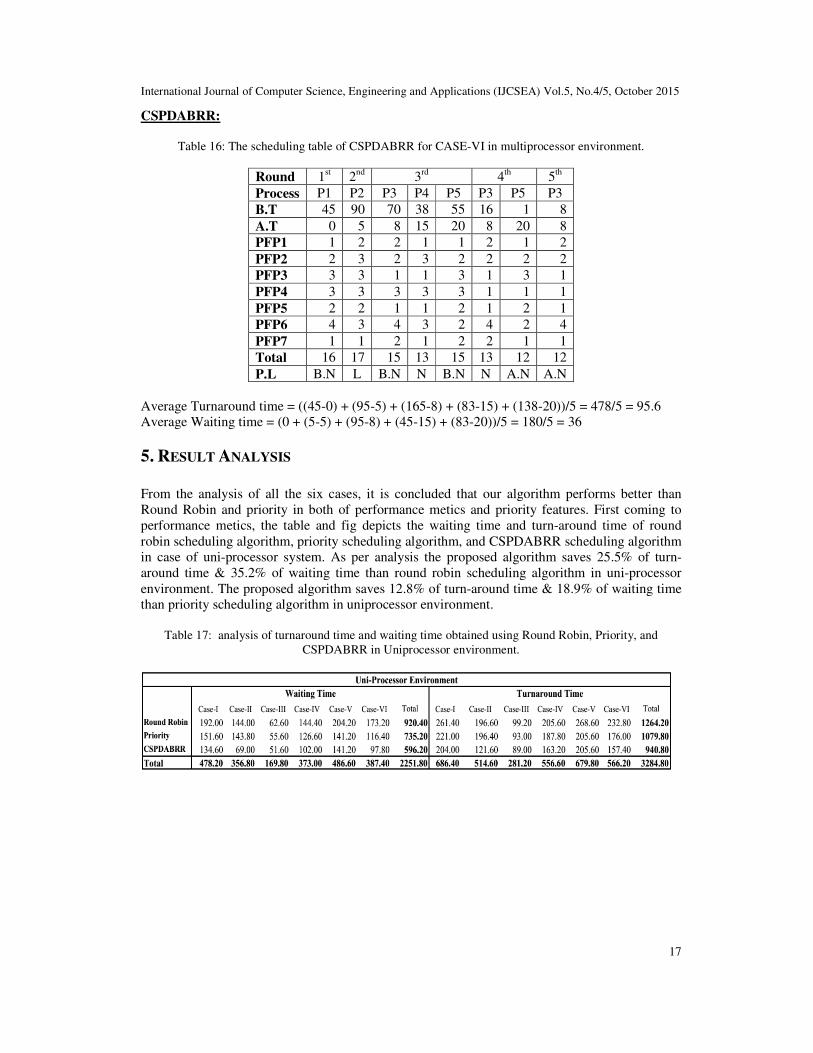
5. RESULT ANALYSIS
From the analysis of all the six cases, it is concluded that our algorithm performs better than
Round Robin and priority in both of performance metics and priority features. First coming to
performance metics, the table and fig depicts the waiting time and turn-around time of round
robin scheduling algorithm, priority scheduling algorithm, and CSPDABRR scheduling algorithm
in case of uni-processor system. As per analysis the proposed algorithm saves 25.5% of turn-
around time & 35.2% of waiting time than round robin scheduling algorithm in uni-processor
environment. The proposed algorithm saves 12.8% of turn-around time & 18.9% of waiting time
than priority scheduling algorithm in uniprocessor environment.
Table 17: analysis of turnaround time and waiting time obtained using Round Robin, Priority, and
CSPDABRR in Uniprocessor environment.
International Journal of Computer Science, Engineering and Applications (IJCSEA) Vol.5, No.4/5, October 2015
18
0
50
100
150
200
250
300
CASE 1 CASE 2 CASE3 CASE 4 CASE 5 CASE 6
Round Robin T.T
Round Robin W.T
Priority T.T
Priority W.T
CSPDABRR T.T
CSPDABRR W.T
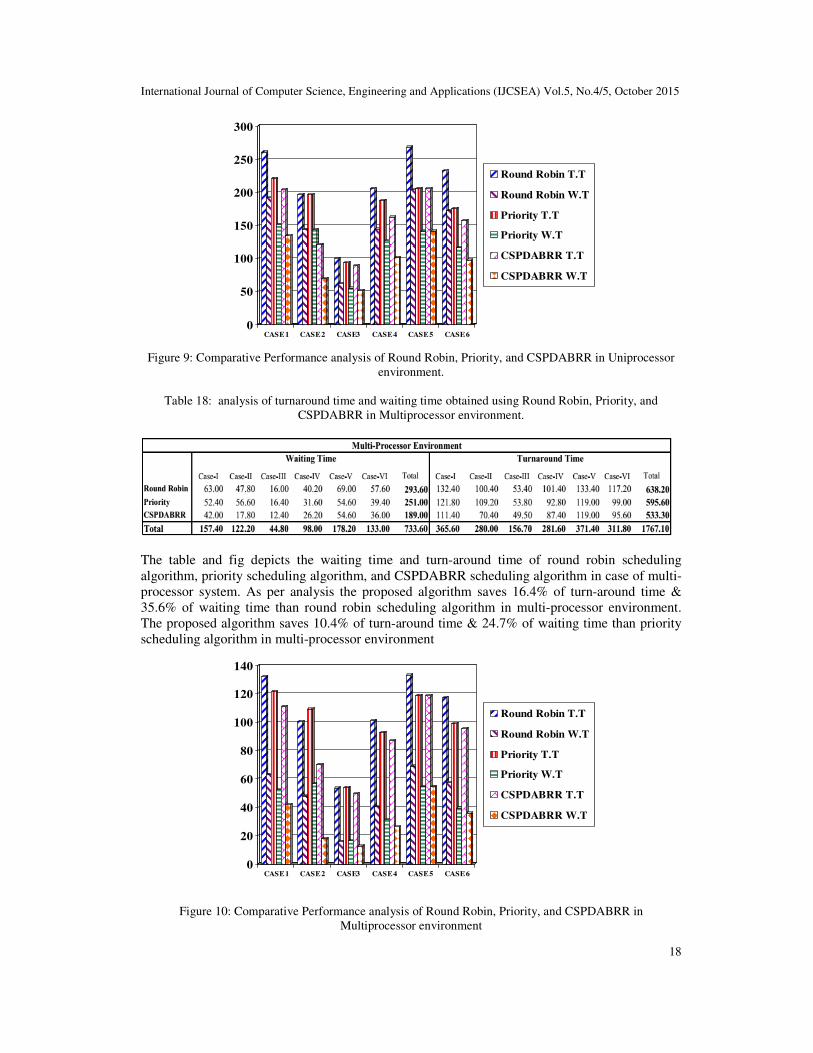
Figure 9: Comparative Performance analysis of Round Robin, Priority, and CSPDABRR in Uniprocessor
environment.
Table 18: analysis of turnaround time and waiting time obtained using Round Robin, Priority, and
CSPDABRR in Multiprocessor environment.
The table and fig depicts the waiting time and turn-around time of round robin scheduling
algorithm, priority scheduling algorithm, and CSPDABRR scheduling algorithm in case of multi-
processor system. As per analysis the proposed algorithm saves 16.4% of turn-around time &
35.6% of waiting time than round robin scheduling algorithm in multi-processor environment.
The proposed algorithm saves 10.4% of turn-around time & 24.7% of waiting time than priority
scheduling algorithm in multi-processor environment
0
20
40
60
80
100
120
140
CASE 1 CASE 2 CASE3 CASE 4 CASE 5 CASE 6
Round Robin T.T
Round Robin W.T
Priority T.T
Priority W.T
CSPDABRR T.T
CSPDABRR W.T
Figure 10: Comparative Performance analysis of Round Robin, Priority, and CSPDABRR in
Multiprocessor environment

International Journal of Computer Science, Engineering and Applications (IJCSEA) Vol.5, No.4/5, October 2015
19
In case of priority, due to inclusion of these seven priority feature points it helps in proper
management of processes according to their features. Our algorithm also helps in load
balancing, deadlock avoidance, and proper utilization of process.
6. CONCLUSIONS
This paper presents the features of CSPDABRR algorithm. This algorithm is integrated of PFPs
for better organization of processes according to their characteristics, features of round robin for
better performance metics. Comparative analysis of RR scheduling algorithm, priority scheduling
algorithm, and the proposed algorithm CSPDABRR has been carried out in both uni-processor
and multi processor environment. The proposed algorithm provides better performance metrics by
minimizing the average waiting time and average turnaround time. it also provide proper load
balancing and proper arrangement of processes according to their features. In future we want to
improve this algorithm by including the concept of multi-threading and processor affinity.
REFERENCES
[1] Abraham Silberschatz, Peter B. Galvin, Greg Gagne (2009) “Operating System Concepts”, eighth edition,
Wiley India.
[2] Neetu Goel, R.B. Garg, (2012) “A Comparative Study of CPU Scheduling Algorithms”, International
Journal of Graphics and Image Processing Volume 2 issue 4, pp 245-251.
[3] Jayashree S. Somani, Pooja K. Chhatwani, (2013) “Comparative Study of Different CPU Scheduling
Algorithms”, International Journal of Computer Science and Mobile Computing, PP 310-318.
[4] Rami J. Matarneh (2009) “Self-Adjustment Time Quantum in Round Robin Algorithm Depending on Burst
Time of the Now Running Processes”, American Journal of Applied Sciences, pp 1831-1837.
[5] Abbas Noon, Ali Kalakech, Seifedine Kadry, (2011) “A New Round Robin Based Scheduling Algorithm
for Operating Systems: Dynamic Quantum Using the Mean Average”, International Journal of Computer
Science Issues (IJCSI), Vol. 8(3), pp 224-229.
[6] H.S.Behera, R. Mohanty, Debashree Nayak, (2010) “A New Proposed Dynamic Quantum with Re-
Adjusted Round Robin Scheduling Algorithm and Its Performance”, International Journal of Computer
Applications, pp 10-15.
[7] Ajit Singh, Priyanka Goyal, Sahil Batra (2010) “An Optimized Round Robin Scheduling Algorithm for
CPU Scheduling”, International journal on Computer Science and Engineering, pp 2383-2385.
[8] Manish Kumar Mishra, Dr. Faizur Rashid (2014) “An Improved Round Robin CPU Scheduling Algorithm
with Varying Time Quantum”, International Journal of Computer Science, Engineering and Applications
(IJCSEA), pp 1-8.
[9] Rishi Verma, Sunny Mittal, Vikram Singh (2014) “A Round Robin Algorithm using Mode Dispersion for
Effective Measure”, International Journal for Research in Applied Science and Engineering Technology
(IJRASET), pp 166-174.
[10] Radhe Shyam, Sunil Kumar Nandal, (2014) “Improved Mean Round Robin with Shortest Job First
Scheduling”, International Journal of Advanced Research in Computer Science and Software Engineering,
PP 170-179.
[11] Amar Ranjan Dash, Sandipta kumar Sahu, Sanjay Kumar Samantra (2015) “An Optimized Round Robin
CPU Scheduling Algorithm with Dynamic Time Quantum”, International Journal of Computer Science,
Engineering and Information Technology (IJCSEIT), Vol. 5,No.1, pp7-26.
[12] Bashir Alam, M.N. Doja, R. Biswas, M. Alam, (2011) “Fuzzy Priority CPU Scheduling Algorithm”,
International Journal of Computer Science Issues (IJCSI), Vol. 8(6), pp 386-390.
[13] H. S. Behera, Ratikanta Pattanayak, Priyabrata Mallick, (2012) “An Improved Fuzzy-Based CPU
Scheduling (IFCS) Algorithm for Real Time Systems”, International Journal of Soft Computing and
Engineering (IJSCE), Vol. 2(1), pp 326-330.
[14] M.Ramakrishna, G.Pattabhi Rama Rao, (2013) “EFFICIENT ROUND ROBIN CPU SCHEDULING
ALGORITHM FOR OPERATING SYSTEMS”, International Journal of Innovative Technology and
Research (IJITR), Vol. 1(1), pp 103-109
[15] Ishwari Singh Rajput, Deepa Gupta, (2012) “A Priority based Round Robin CPU Scheduling Algorithm for
Real Time Systems”, International Journal of Innovations in Engineering and Technology (IJIET), Vol.
1(2), pp pp 1-11.
International Journal of Computer Science, Engineering and Applications (IJCSEA) Vol.5, No.4/5, October 2015
20
[16] H.S.Behera, Sabyasachi Sahu, Sourav Kumar Bhoi, (2011) “Weighted Mean Priority Based Scheduling for
Interactive Systems”, Journal of Global Research in Computer Science, Vol. 2(5), pp 1-7.
[17] H.S. Behera, Simpi Patel, Bijayalakshmi Panda, (2011) “A New Dynamic Round Robin and SRTN
Algorithm with Variable Original Time Slice and Intelligent Time Slice for Soft Real Time Systems”,
International Journal of Computer Applications, Vol. 16(1), PP.
[18] Rakesh Mohanty, H. S. Behera, Khusbu Patwari, Monisha Dash, M. Lakshmi Prasanna, (2011) “Priority
Based Dynamic Round Robin (PBDRR) Algorithm with Intelligent Time Slice for Soft Real Time
Systems”, International Journal of Advanced Computer Science and Applications (IJACSA), Vol 2(2), PP
46-50.
[19] Zena Hussain Khalil, Ameer Basim Abdulameer Alaasam, (2013) “Priority Based Dynamic Round Robin
with Intelligent Time Slice and Highest Response Ratio Next Algorithm for Soft Real Time System”,
Global Journal of Advanced Engineering Technologies, Vol 2(3), pp 120-124.
[20] H.S. Behera, Jajnaseni Panda, Dipanwita Thakur, Subasini Sahoo, (2011) “A New Proposed Two Processor
Based CPU Scheduling Algorithm with Varying Time quantum for Real Time Systems”, Journal of Global
Research in Computer Science, Vol. 2(4), pp 81-87.
AUTHORS
Amar Ranjan Dash has achieved his B. Tech. degree from Biju Patnaik University of
Technology, Odisha, India and M. Tech. degree from Berhampur University, Odisha, India.
His research interests include CPU Scheduling, Web Accessibility, and Cloud Computing.
Sandipta Kumar Sahu has achieved his B. Tech. degree from Biju Patnaik University of
Technology, Odisha, India and M. Tech. degree in computer science and engineering at
National Institute of Science And Technology, Odisha, India. His research interests include
Operating System, Software engineering, and Computer Architecture.
Sanjay Kumar Samantra has achieved his MCA degree from Berhampur University, Odisha,
India and M. Tech. degree in computer science and engineering at National Institute of
Science And Technology, Odisha, India. His research interests include CPU scheduling,
Grid computing, and Cloud Computing.
Sradhanjali Sabat has achieved her B.Tech degree from The Techno School, Odisha, India
and M. Tech. degree in computer science and engineering at National Institute of Science
And Technology, Odisha, India. Her research interests include wireless sensor networks ,
computer networks.