D/2005/6482/29

Vlerick Leuven Gent Working Paper Series 2005/29

CHARACTERISATION AND GENERATION OF NURSE SCHEDULING

PROBLEM INSTANCES

MARIO VANHOUCKE

Mario.Vanhoucke@vlerick.be

BROOS MAENHOUT

2

CHARACTERISATION AND GENERATION OF NURSE SCHEDULING

PROBLEM INSTANCES

MARIO VANHOUCKE

Vlerick Leuven Gent Management School

BROOS MAENHOUT

Ghent University

Contact:

Mario Vanhoucke

Vlerick Leuven Gent Management School

Tel: +32 09 210 97 81

Fax: +32 09 210 97 00

Email: Mario.Vanhoucke@vlerick.be

3

ABSTRACT

In this paper, we propose different complexity indicators for the well-known nurse

scheduling problem (NSP). The NSP assigns nurses to shifts per day taking both hard and

soft constraints into account. The objective is to maximize the nurses’ preferences and to

minimize the total penalty cost from violations of the soft constraints. The problem is

known to be NP-hard.

Due to its complexity and relevance in practice, the operations research literature has been

overwhelmed by different procedures to solve the problem. The complexity has resulted in

the development of several (meta-)heuristic procedures, able to solve a NSP instance

heuristically in an acceptable time limit. The practical relevance has resulted in a never-

ending amount of different NSP versions, taking practical, case-specific constraints into

account.

The contribution of this paper is threefold. First, we describe our complexity indicators to

characterize a nurse scheduling problem instance. Secondly, we develop a NSP generator to

generate benchmark instances to facilitate the evaluation of existing and future research

techniques. Finally, we perform some preliminary tests on a simple IP model to illustrate

that the proposed indicators can be used as predictors of problem complexity.

Keywords: Nurse scheduling; Benchmark instances; Problem classification

4

1. INTRODUCTION

The nurse scheduling problem (NSP) is a well-known combinatorial optimization

problem in literature and has attracted numerous researchers to develop exact and (meta-)

heuristic procedures. The NSP involves the construction of duty rosters for nursing staff

and assigns the nurses to shifts per day taking both hard and soft constraints into account.

The objective maximizes the preferences of the nurses and minimizes the total penalty cost

from violations of the soft constraints. The problem is known to be NP-hard (Osogami and

Imai, 2000).

Despite the numerous procedures for the NSP, no state-of-the art results have been

presented in literature. The main reason is that comparison between procedures is very

difficult, since problem descriptions and models vary drastically and depend on the need of

the particular hospital. Due to the huge variety of hard and soft constraints, and the several

objective function possibilities, the nurse scheduling problem has a multitude of

representations, and hence, a wide variety of solution procedures has overwhelmed the

optimization literature. The comparison is further hindered by the lack of benchmark

problem instances and the unavailability of source code of the different procedures.

Moreover, there is no general agreement on how to evaluate and compare procedures in

terms of solution comparison, stop criterion, etc…. Consequently, a fair comparison

between procedures seems to be an impossible idea, which undoubtedly limits the efficient

development of future algorithms.

In their overview papers, Cheang et al (2003) and Burke et al (2004) express the

need for a benchmark database to facilitate comparison of the various algorithms and to

motivate future researchers to develop better solution procedures for the NSP. In this paper,

we come towards this need of benchmarking in several ways.

The outline of the paper is as follows. In the next section, we briefly review the use

of hard and soft constraints applicable to nurse scheduling problems. Section 3 presents the

complexity indicators for the NSP that are used as a base for the problem instance generator

(NSPGen). In section 4 we present our generation approach to generate problem instances

under a controlled design. In section 5, we report the relevance of these indicators by

computational results on a simple IP model. A decision tree has been constructed to

5

distinguish groups of data instances based on known input parameters. Section 6 draws

overall conclusions and suggestions for future research avenues.

2. THE NSP UNDER DIFFERENT ASSUMPTIONS

The basic nurse scheduling problem (NSP) can be stated as follows. A set of nurses

needs to be scheduled within a pre-defined period (e.g. a week). In doing so, these nurses

need to be assigned to one of a number of possible shifts in order to meet the minimal

coverage constraints and other case-specific constraints and to maximize the quality of

assigned working shifts. According to Warner (1976), quantifying preferences in the

objective function maintains fairness in scheduling nurses over the scheduling horizon.

Hence, the quality of a schedule is a subjective judgment of the nurses depending on how

well the assigned schedule is conform to his/her desires to be off or on duty and to other

schedule properties such as work stretch, rotation patterns, etc…. The coverage constraints

determine the required nurses per shift and per day, and are inherent to each NSP instance.

However, many other constraints are very case-specific, and are determined by personal

time requirements, specific workplace conditions, national legislation, etc…. The majority

of these extra constraints can be handled as hard constraints, for which no violation is

possible whatsoever, or as soft constraints, which can be violated at a certain penalty cost.

In their literature survey, Cheang et al (2003) present an overview of constraint types as

appearing frequently in the literature. In the remainder of our paper, we propose different

complexity indicators to describe a NSP instance. More precisely, these indicators describe

a two-dimensional nurse/day preference roster and the corresponding coverage

requirements, which are both inherent to any NSP instance. We assume a nurse scheduling

problem where each nurse i can express its preference to work on day j in shift k as pijk. We

opt for this general approach to express the preference or aversion of nurses to work on a

shift/day, and hence, ignore some very case-specific preference structures, such as

sequence-dependent preferences. We believe, however, that most nurse scheduling

problems can be modelled by using our general preference matrix. The required number of

nurses (coverage requirements) on day j for shift k can be denoted by rjk.

6

The objective is to schedule the nurses for the complete period, such that the

coverage requirements are met and the total sum of nurses’ preferences and the penalty

costs of soft constraints violations are minimized.

3. NSP GENERATION

In this section, we present three classes of complexity indicators in order to generate

NSP instances under a controlled design. These complexity indicators should span the full

range of problem complexity and should have sufficient discriminatory power to serve as

predictors for the complexity of the problem under study (Elmaghraby and Herroelen,

1980). Hence, it allows the generation of instances with pre-defined values for the

complexity indicators to predict the difficulty of a particular NSP instance for a particular

solution procedure. Therefore, different sets with different combinations of the indicators

can discriminate between easy and hard instances and these indicators can act as predictors

of the computational effort of the procedures that have been developed. The CPU-time that

a solution procedure needs to solve a particular problem instance to optimality can typically

be used to describe the hardness of this problem instance for the particular solution

procedure. Hence, the comparison of procedures and good predictions of their required

CPU-time allow the a priori selection of the fastest solution procedure, based on the simple

calculation of the indicators. The complexity indicators are therefore indispensable in the

construction of problem sets that span the complete range of complexity of important

problem characteristics.

Insert Table 1 about here

The three classes of proposed complexity indicators to generate a NSP instance

measure the size of the problem instance, the preference structure of the nurses and the

coverage requirements of the schedule. Table 1 serves as a guideline to following sections,

where the three classes of indicators will be explained into detail.

7

3.1. Problem size

The size of the NSP instance under study depends on the size of the duty roster

matrix. Consequently, the three complexity indicators describing the size of the problem

can be defined as:

N = number of nurses

S = number of shifts

D = number of days

These three input parameters will be used to describe the two following classes of

complexity indicators. The preferences have to be expressed by each nurse, for each shift of

all days (see section 3.2). The coverage requirements need to be given for all shifts of all

days (see section 3.3).

3.2. Preferences

The preference structure of the nurses consists of three input parameters. First, the

preference distribution over all nurses (for each shift and for each day) needs to be

determined by the nurse-preference distribution. Second, these preferences need to be

distributed among all shifts of a single day, denoted by the shift-preference distribution.

Last, the preference distribution for all days of the complete scheduling period needs to be

determined, referred to as the day-preference distribution. In doing so, we have full control

on the complete preference distribution for all nurses for each shift on each day.

3.2.1. Nurse-preference distribution (NPD)

We assume that a shift/day preference can be expressed by nurses as a ranking

among shifts. More precisely, each nurse can rank each possible working shift of the day,

such that the maximal number of different preference values equals the number of shifts S.

In doing so, each nurse expresses his/her desire to work on that particular shift by assigning

a number between 1 (very desirable) and S (very undesirable). The NPD measures the

distribution of the preferences over all nurses for a particular shift on a particular day. In the

remainder of this section, we explain the calculation of the NPD measure for a particular

8

shift k of a particular day j. Although the NPD value can differ for each shift of each day,

we assume that the nurse-preference distribution is equal for all shifts and all days.

We introduce an auxiliary variable to measure the number of times an identical

preference value l (l = 1, …, S), has been selected for a particular shift and day among the

nurses, as follows:

yil = 1, if nurse i prefers choice l (for a particular shift on a particular day)

0, otherwise

and hence,

N

i

ily1

denotes the number of times a ranking value l has been selected

by all the nurses for a particular shift/day.

NPD [0, 1] can be calculated as NPD

S

l

N

i

il

NPD

NPD

w

SNy

NPDmax

1 1

max

/

.

Consequently, NPD

w measures the total absolute deviation of all

N

i

ily1

-values for

each preference l from the average number of each preference, i.e. N / S. Indeed, since the

total number of different preferences equals S, each preference will be selected N / S times,

on the average. Moreover, NPD

max is used to denote the maximal possible value of NPD

w . By

dividing NPD

w by NPD

max , we make sure that NPD lies between zero and one, inclusive. The

value for NPD

max depends on the maximal allowable value for

N

i

ily1

which is equal to N, and

can be expressed as S

NN

22 . For more information, we refer to appendix A. In this

appendix, we show that our variance measure NPD

NPD

w

max

is a general measure for the

distribution of any parameter which will also be used in this paper to describe other

complexity indicators. It has been proposed by Vanhoucke et al (2004) for the generation of

9

project networks and has been adapted by Labro and Vanhoucke (2005) to design general

costing systems for management accounting.

The NPD measures whether the preference structure is distributed equally over the

nurses (there is no clear preference among the nurses for this particular shift, or NPD = 0)

or shows a clear pattern for one preference (all nurses have the same ranking value for that

shift, or NPD = 1). In table 2, we display three different NPD values for three shifts (k = 1,

2 or 3) and 15 nurses. As an example, NPD1 = (|13 – 5| + |1 – 5| + |1 – 5|) / (2 * 15 – (2 * 15

/ 3)) = 0.80, denoting that the majority of nurses (13) have shift 1 as their first choice (and 1

nurse as the second choice and 1 nurse as the last choice). The NPD only measures the

distribution of preferences among nurses, but does not assign the individual preferences of

the generated distribution to particular shifts of a particular day. The shift-preference

distribution indicator of section 3.2.2 and the day-preference distribution indicator of

section 3.2.3 assigns the individual preferences among shifts and days, respectively. As an

example, table 3 displays a preference matrix for which the NPD-values equal 0.80 for the

first shift of each day, 0.50 for the second shift of each day and 0.20 for the third shift of

each day.

Insert Table 2 about here

3.2.2. Shift-preference distribution (SPD)

The NPD measures the distribution of the preferences l (expressed as a ranking

value between 1 and S) among nurses, but does not assign the individual preference values

to individual nurses to express his/her desire to work on that shift of that day. The SPD

assigns these preferences to nurses and measures the distribution of these preferences over

all shifts of a single day. Although the SPD value can differ for each day, we assume that

the shift-preference distribution is equal for all days over the complete scheduling horizon.

SPD [0, 1] can be calculated as NS

N

SPD

N

i

SPD

i

)1(

1

.

10

SPD

i measures the number of different preference values for nurse i over all shifts k

of a particular day. Using P as a temporary set for preference ranking values, SPD

i can be

calculated for each nurse i as follows:

SPD

i = 0

P =

for k = 1, …, S

if (pijk P) then

SPD

i = SPD

i + 1

P = P pijk

where pijk–values can vary between 1 and S.

A minimal value for SPD

i equals 1 when nurse i expresses no clear preference

among the shifts (and hence, assigns a similar preference value to each shift of the day to

express indifference among shifts). The maximal value for SPD

i equals S and means that

nurse i has a clear ranking between each shift on a day. Consequently, the maximal value

for

N

i

SPD

i

1

equals SN and minimal value equals N and the SPD always lies between zero

and one, inclusive. The SPD measures the preference structure over all shifts within a day

and equals 0 if all nurses express indifference between the shifts and equals 1 if each nurse

expresses a preference ranking among the individual shifts. As an example, table 3 displays

the four-days preference matrix with a SPD-value equal to 0.2 for day 1, 0.4 for day 2, 0.6

for day 3 and 0.8 for the last day. Note that the NPD equals 0.8, 0.5 or 0.2 for the first,

second or third shift, respectively, for each day.

3.2.3. Day-preference distribution (DPD)

The SPD of previous section can be applied to each day of the complete scheduling

period in order to control the preference structure over all shifts of each day. In order to

11

control the preference structure over all days of the complete scheduling period, an

indicator to measure the day-preference distribution is necessary.

The DPD indicator is similar to the SPD, but measures the distribution of the

preferences over all days, instead of a single-day distribution over all shifts. In analogy with

SPD

i , DPD

ik measures the number of different preference values for nurse i on shift k over

all days.

DPD [0, 1] can be calculated as NSS

NS

DPD

N

i

S

k

DPD

ik

)1(

1 1

.

Since the maximal value for

N

i

S

k

DPD

ik

1 1

equals SSN and minimal value equals SN,

the DPD always lies between zero and one, inclusive. When DPD equals 0, then all nurses

have expressed a similar preference or aversion for similar shifts over all days. On the other

hand, DPD equals 1 when each nurse has assigned a different preference value for similar

shifts over the days (i.e. the nurses have clearly a day-dependent preference for each shift).

The DPD-value for table 3 equals 0.70.

In order to clarify the different indicators, we have displayed some extreme

preference structures measured by the three preference distribution measures in appendix B.

3.3. Coverage constraints

The coverage requirements, expressed as the required number of nurses on day j for

shift k, will be expressed as rjk. Furthermore, we use S

r

r

S

k

jk

j

1 to denote the average

number of nurses required per shift on day j and D

r

r

D

j

S

k

jk

1 1

to denote the average

12

number of nurses required per day. The coverage requirements of the nurse scheduling

problem can be generated by means of three input parameters as follows. In a first step, the

total number of required nurses will be generated which has a major influence on the

constrainedness and hence on the feasibility of the NSP instance. In a second step, the total

number of required nurses will be distributed among the days (day-coverage) and the shifts

per day (shift-coverage).

3.3.1. Total-coverage constrainedness (TCC)

The TCC serves as an indicator to generate the total number of nurses required for

the complete scheduling period (e.g. a week). The required number of nurses (i.e. the

coverage requirements) as well as the different case-specific constraints have a major

influence on the feasibility of the NSP instance under study. An NSP instance with only the

coverage requirement constraints has a feasible schedule when the total daily coverage is

lower than or equal to the number of nurses. Hence, the maximal allowable daily coverage

is equal to the number of nurses in the instance, and higher coverage values will lead to

infeasible solutions. However, the feasibility can no longer be guaranteed when the NSP

instance is subject to additional constraints. For these instances, the total coverage needs to

be decreased (lower than the number of nurses) and, therefore, can only be a fraction of the

maximal coverage. Note that Koop (1988) has discussed lower bounds for the workforce

size on the multiple shift manpower scheduling problem by taking both the minimal

number of required working shifts (i.e. the coverage constraints) as well as other case-

specific constraints into account.

The TCC [0, 1] can be calculated as N

r

ND

r

TCC

D

j

S

k

jk

1 1

.

The total-coverage constrainedness (TCC) is measured as the average number of

nurses required per day divided by the number of nurses. The TCC is measured as a fraction

of the maximal coverage requirements (when the TCC = 1, the total daily coverage equals

the number of nurses). When the NSP instance is the subject to additional constraints, the

13

TCC needs to be lower than or equal to 1 to guarantee feasibility. The TCC value of table 3

equals (3 + 3 + 3 + 1 + 2 + 3 + 4 + 1 + 1 + 0 + 9 + 0) / (15 * 4) = 0.5.

3.3.2. Day-coverage distribution (DCD)

The TCC determines the total coverage requirement for the complete scheduling

period but does not assign requirements to individual days or shifts. The DCD divides the

total coverage requirement (obtained by the TCC measure) among days in a controlled way

as follows:

DCD

D

j

S

k

jk

DCD

DCD

w

rr

DCDmax

1 1

max

The DCD is similar to the SPD indicator as explained in appendix A. DCD

w

measures the total absolute deviation of a one-day coverage

S

k

jkr1

from the total average

coverage requirement over all days. Moreover, DCD

max is used to denote the maximal

possible value of DCD

w . Similar to the SPD indicator of section 3.2.1, we divide DCD

w by

DCD

max to make sure that DCD lies between zero and one, inclusive. The value for DCD

max

depends on the maximal allowable value for

S

k

jkr1

(which is equal to N) and is equal to

rNrDDrN

rDrN

mod)1(2 (see appendix A).

DCD measures whether the daily coverage is distributed equally over all days, and

does not measure the intra-day coverage requirement over the shifts. When DCD is equal to

0, the coverage requirements are equally distributed among all days. When DCD equals 1,

the coverage requirements are maximal for one or several days (depending on the TCC

value), and zero for all remaining days. The DCD value of table 3 equals DCD = (|9 – 7.5| +

14

|6 – 7.5| + |6 – 7.5| + |9 – 7.5|) / ((15 – 15) *

15

5.7*4– 7.5 * (1-4) + |(4 * 7.5)mod(15) –

7.5|) = 6 / 30 = 0.2.

3.3.3. Shift-coverage distribution (SCD)

While the DCD measures the daily coverage distribution over the complete

scheduling problem, the SCD does the same, on a shift level. More precisely, the SCD

measures the distribution of the coverage requirements over all shifts for a particular day j.

Although the SCD indicator can differ per day, we assume that the shift-coverage

distribution is equal for all days.

The SCD [0, 1] can be calculated as SCD

S

k

jjk

SCD

SCD

w

rr

SCDmax

1

max

.

Similar to SPD and DCD, SCD

w measures, for a given day j, the total absolute

deviation of all shift coverage requirements rjk from the total average coverage requirement

of that day (which is a result of the DCD calculations). SCD

max is used to denote the maximal

possible value of SCD

w and depends on the maximal allowable value for jkr . This maximal

value equals N, and can never be exceeded since the DCD calculations guaranteed that

NrS

k

jk 1

. Therefore, no explicit upper value needs to be taken into consideration, and

SCD

max can be – according to appendix A – calculated as jj rrS 22 . When SCD equals 0,

the coverage requirements for a single day are equally distributed. When SCD equals 1,

there is a single shift with a given coverage requirement (determined by the DCD

indicator), while all other shifts on that day do not need nurses. The SCD values of table 3

equal 0, 0.25, 0.5 and 1 for day 1, 2, 3 and 4.

15

4. THE GENERATION PROCESS OF THE NSP INSTANCE GENERATOR

NSPGEN

In this section, we describe a simple but efficient way to generate NSP instances

with given values for the 9 indicators of section 3. In the remainder of this section, we refer

to a ‘shift vector’ to denote one column of a preference matrix as shown in table 3.

Moreover, we refer to a day matrix (week matrix) to denote a combination of shift vectors

for a complete day (week). We describe our generation approach for weekly preference

matrices, but it can easily be extended, without loss of generality, to larger scheduling

periods.

The generation process boils down to the combination of randomly generated shift

vectors with a pre-specified NPD value in order to obtain a preference structure with known

values for all the indicators. This process is followed by an improvement step, until a pre-

specified value for SPD and DPD is obtained. The pseudo-code to generate periodically

(e.g. weekly) preference matrices with a given value for NPD, SPD and DPD (denoted as

NPD’, SPD’ and DPD’) is given below.

Procedure Generate instance (NPD’, SPD’, DPD’)

Initialize d1 = 0

Step 1. Construct NPD’ shift vectors

Randomly generate C1 shift vectors with NPD’-value

Step 2. Construct D1 SPD’ day matrices

Select randomly one shift vector c1 from the C1 vectors Construct a day matrix with SPD = 0 (i.e. all shifts equal c1)

Set SPDold = 0

For k = 2 to S

For c2 = 1 to C1

Replace shift vector c1 with vector c2 for shift k

and calculate SPDnew

If |SPD’ - SPDnew| < |SPD’ – SPDold| then

Replace vector c1 with vector c2

SPDold = SPDnew

Save the day matrix and set d1 = d1 + 1

If d1 < D1 repeat step 2

Step 3. Construct W1 DPD’ week matrices

Select randomly one day matrix d1 from the D1 matrices Construct a week matrix with DPD = 0 (i.e. all days equal d1)

Set DPDold = 0

For j = 2 to D

For d2 = 1 to D1

Replace day matrix d1 with matrix d2 for day j

and calculate DPDnew

If |DPD’ - DPDnew| < |DPD’ – DPDold| then

16

Replace matrix d1 with matrix d2

DPDold = DPDnew

Save the week matrix and set w1 = w1 + 1

If w1 < W1 repeat step 3

Step 4. Improvement SPD’ and DPD’

Select the best found week matrix with known SPD and DPD value

For j = 1 to D

For k = 1 to S

For i1 = 1 to N

For i2 = i1 to N

Swap(pi1,j,k, pi2,j,k)

If SPD or DPD improves, save new week

matrix

Return

The first step randomly generates C1 shift vectors with a NPD-value as close as

possible to NPD’ (a shift vector is one column of a week preference matrix as given in table

3). In step 2, the procedure combines these vectors to generate a day preference matrix with

a given value for SPD’. To that purpose, the procedure randomly selects one shift vector

and creates a day matrix with a SPD-value of 0. This day matrix contains the selected shift

vector for all shifts of the day. The procedure aims at improving the SPD-value by

replacing the shift vectors one at a time with the other generated shift vectors of step 1.

Each time an improvement has been made (i.e. the newly found SPD value lies closer to the

pre-specified SPD’-value), the new shift vector replaces the old one in the day matrix. The

best found day matrix will be saved and this process will be repeated until D1 day matrices

are obtained. In step 3, these day matrices, on their turn, are used to combine them to week

matrices with a given DPD’-value in a similar way as the construction of the day matrices.

Instead of scanning all the shifts (step 2), the procedure scans all the days to find good

combinations of day matrices to result in week matrices with a DPD-value close to DPD’.

This process is repeated until W1 week schedules are obtained. Step 4 selects the best week

matrix found and aims at improving the DPD and SPD value. More precisely, the procedure

swaps individual nurse preferences for each day and each shift in order to look for

improvement for SPD and DPD. The NPD value remains unchanged during this step, since

swaps are made within one single shift. Computational tests have revealed that a stop

criterion C1 = D1 = W1 = 100 for each step results in a fast and efficient procedure with

excellent performance for all indicators. All preference matrices are extended with coverage

17

requirements by the controlled random generation of numbers with known values for the

TCC, SCD and DCD indicators.

In their overview papers, Cheang et al (2003) and Burke et al (2004) call the

importance of benchmark instances to test the exact and/or (meta-)heuristic procedures for

the nurse scheduling problem. In doing so, a benchmark dataset that is shared among the

research community facilitates the systematic evaluation and comparison of the

performance of the different procedures. The proposed instance generator NSPGen is a

useful tool to generate these instances based on the set of complexity indicators proposed in

section 3. Hence, a library of NSP instances (NSPLib) has been presented by Vanhoucke

and Maenhout (2005) that is accessible by the research community. The benchmark

instances have been grouped in six different sets and are characterized by systematically

varied levels of all the complexity indicators. In total, NSPLib contains 7,290 problem

instances with a one-week scheduling period and 1,920 instances with a one-month

scheduling period. Each instance of the dataset can be extended by a particular set of case-

specific constraints. More precisely, the user can choose among 16 sets of possible

constraints, where each set consists of a combination of constraints identified by Cheang et

al (2003) as appearing frequently in literature. For more details about the proposed

benchmark set, we refer the reader to Vanhoucke and Maenhout (2005). The problem

instances and the corresponding case constraint files can be downloaded from

www.projectmanagement.ugent.be/nsp.php.

5. COMPUTATIONAL EXPERIMENTS

5.1. Preliminary test results

Small sized nurse scheduling problems can be solved using branch and bound

procedures typically provided with commercially available software. We have programmed

a simple IP model to solve small instances of the NSP procedures in Visual C++ version 6.0

and run it on a Toshiba personal computer with a Pentium IV 2.4 GHz processor under

Windows XP. The model has been linked with the industrial LINDO optimization library

version 5.3 (Schrage, 1995). In this paper, we do not have the intention to present an

18

efficient model to solve large-sized realistic nurse scheduling problem instances. Instead,

we aim at detecting the influence of preference structures and coverage requirements with

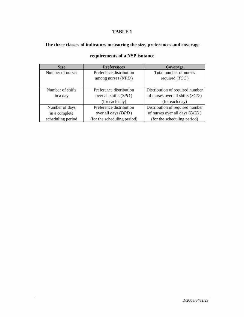
given values of the pre-defined indicators on the problem complexity. To that purpose, we

have generated small-sized NSP instances with the complexity indicators as given in table

4. Using 5 instances for each problem class, we obtain 46,875 data instances.

Insert Table 4 about here

The simple IP model contains the following case-specific constraints:

Number of assignments per nurse equals 5

minimum 2 consecutive working days per nurse

minimum 2 identical consecutive working shifts per nurse

The hardness of a problem instance is typically measured by the amount of CPU-

time that a solution procedure needs to find an exact solution for the problem at hand. It is

therefore of great importance to possess a set of problem characteristics that discriminates

between easy and hard instances and that acts as a predictor of the computational effort of

the procedures. If good predictions of the required CPU-time for different solution

procedures were available, it would be possible to a priori select the fastest solution

procedure, based on the simple calculation of these problem characteristics. The following

tables display the average CPU time (Avg.) required to solve the problem instances to

optimality and the number of instances for which a feasible solution exists (#Sol). Each

table contains the required CPU time for the complexity indicators (either preference

related or coverage related) and the number of instances that could be solved to optimality

within a pre-determined time of 180 seconds.

Table 5 displays the one-dimensional effect of the six indicators on the required

CPU-time to solve the problem instances to optimality. Tables 5, 6, 7 and 8 clarify the

effects of the different indicators on problem complexity (measured by the CPU-time).

19

Insert Table 5 about here

The effect of NPD shows an increasing pattern on the CPU-time. Indeed, the more

nurses express an identical preference for a particular shift, the more conflicts between

nurses exist, resulting in an increasing problem complexity.

The SPD shows a hard-easy-hard transition effect, and has been further explained in

combination with NPD, as shown in table 6. For low NPD values, the table shows a

decreasing effect for increasing SPD-values. In general, low NPD values results in a few

conflicts between nurses, and hence, in a rather easy schedule. Combined with high SPD

values results in a clear nurse preference for each shift of the day and hence, there are not

much conflicts, neither between the different nurses nor between their shift preferences on

each day. However, a low SPD value means that nurses are indifferent between shifts, and

hence it is not a priori clear which shift assignment is best for each nurse. The table shows

an opposite behaviour for high NPD values (which result in a higher complexity anyway).

Both low and high SPD values results in a conflict between nurses. In the former, all nurses

have an identical preference for all shifts, and hence, a switch for a nurse to another shift

does not influence the total preference cost but might resolve some case-specific constraint

violations. High SPD values results in a clear conflict between the shifts, since all nurses

express an identical preference for each shift. As a result, the (preference) cost of switching

a particular nurse to his/her second or third choice results in an increase of the preference

cost. The effect between NPD and DPD shows a similar behaviour as table 6, although

somewhat less outspoken, as shown in table 7.

Insert Table 6 and Table 7 about here

The TCC measures the constrainedness of the problem instances, and has a positive

correlation with problem complexity. If more nurses are required by the hospital, then the

freedom to schedule a subset of nurses on a particular shift/day without violating case-

specific constraints is dramatically reduced. Increasing values for DCD result in an

20

increasing complexity. Table 8 further clarifies the effect of DCD on the CPU-time, in

combination with the different settings for the TCC complexity indicator.

Insert Table 8 about here

This table reveals that the DCD has a negative impact on the CPU-time for low

TCC-values, and an opposite behaviour for medium or high values for TCC. Low TCC-

values and high DCD values result in tight coverage requirements for a small number of

days while all other days do not require any nurses. Hence, only a small number of days are

constrained, which results in much freedom to schedule the nurses over the complete time

horizon. On the other hand, high DCD values with high TCC values result in tight coverage

requirements for almost all days. Hence, a careful trade-off needs to be made to schedule

the nurses without violating many case-specific constraints.

The effect of SCD shows, in general, an easy-hard-easy transition, i.e. an increasing

(from low to medium values) followed by a decreasing (from medium to high values)

effect, on the CPU-time. Low SCD values mean that the coverage requirements are almost

equally distributed among the shifts, and hence, the probability of violating case-specific

constraints (like the consecutiveness constraints) is rather low. As the SCD value goes up,

violating these constraints is more likely, resulting in a higher problem complexity.

However, large values for SCD either results in easy schedules or infeasible schedules,

which explains the decreasing trend of the CPU-time. Indeed, all daily nurse requirements

occur on one single shift, which results in either an almost unconstrained problem instance

(there is no much choice than assigning nurses to this shift) or infeasible instances (due to

the limited choice and the consecutiveness and succession constraints, no feasible

assignment can be found). In appendix C, we tested the significance of the mean differences

by means of a one-way ANOVA test. Moreover, we extended the table by a post hoc

analysis to detect which mean values are different. The appropriate post hoc test was

selected based on the homogeneity of variances indicated by Levene's test for homogeneity

of variances.

21

5.2. A CHAID regression tree

In order to gain further insights on the influence of the proposed indicators on

problem complexity, we clustered our data instances based on the required CPU-time in a

way that reduces variation. This categorization is performed using a decision tree based on

the CHAID algorithm (Chi-square automatic interaction detection (Kass, 1980)) of which

the goal is to create a concise model which a priori predicts the hardness of new problem

instances based on their characteristics. CHAID investigates the effects of independent

variables on a dependent variable. Starting with all observations in a single group and a set

of independent variables, the observations are subsequently split into two or more groups

by the same or an alternative independent variable until further splitting will not reduce the

variation of the dependent variable. The splitting is performed by the independent variable

that is judged to be most important in reducing the total variation in the dependent variable.

The criterion for evaluating a splitting rule is based on a statistical significance test, namely

an F-test with a p-value of 0.05 as a stopping rule. Furthermore, the split is performed

subject to a limit of 5 branches (which is equal to the (maximal) number of different values

for each indicator of table 4) and a limit of minimal 10 observations assigned to each

branch. For these criteria, the best split is the one with the smallest p-value. The decision

tree, presented in appendix D, is created using a training data set (records sampled from the

entire dataset of table 4) and validated on a testing dataset (remaining records). The dataset

was randomly split into a training and a testing dataset, 70 – 30 respectively. For each split

the splitting variable and the resulting branches with their corresponding split values are

indicated. The tree counts 29 splitting nodes and 49 end nodes (leaves) which are

designated by a number. The descriptive statistics (average; standard deviation) for the

leaves are indicated below the tree.

In order to visualize the discriminative power and to give an indication of the

predictive power of the decision tree, we generated new data instances by NSPGen based

on the values for the complexity indicators for 10 different end nodes. Furthermore, we

generated data instances with neighbouring values for some of these classes. The data

instances of classes 11, 12, 13 and 14 are created in the vicinity of classes 2, 3, 9 and 10,

respectively (and hence, the “end node” column values correspond to each other). The

22

values for the complexity indicators for newly generated problem instances for the

designated end nodes are indicated in table 9.

Insert Table 9 about here

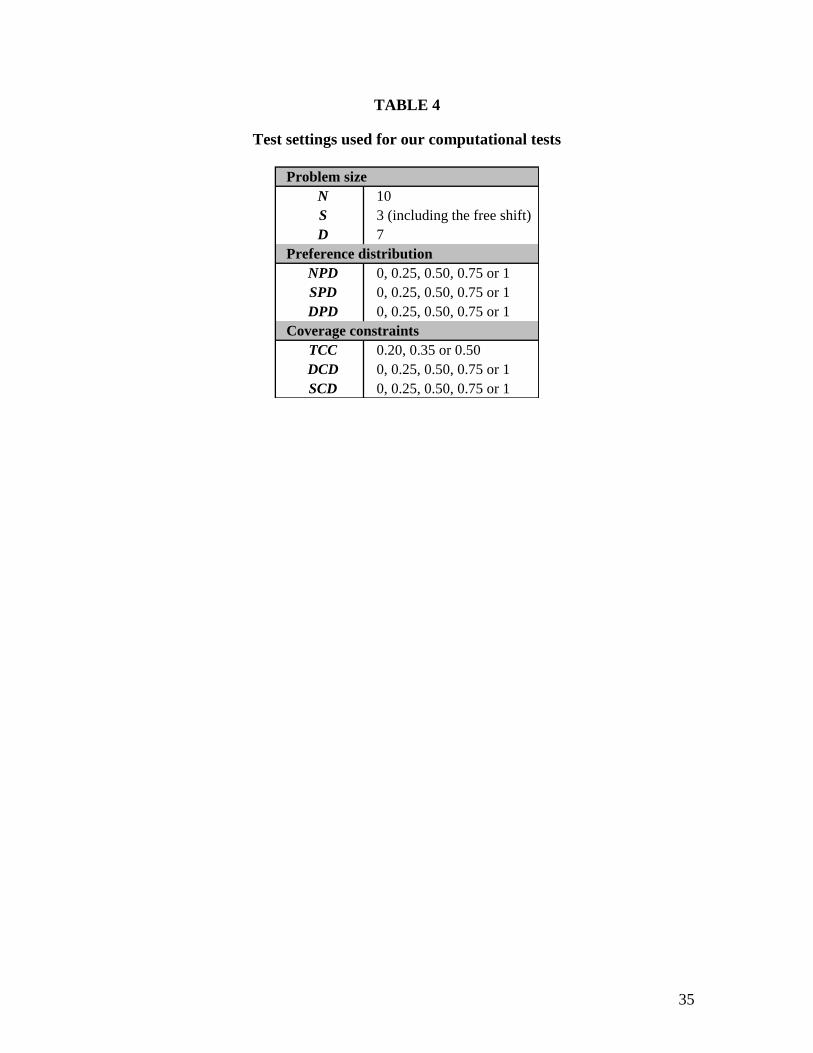
The required CPU-time to solve these data instances to optimality are presented in

figure 1. This figure reveals that instances within a class are rather homogeneous with

respect to the computational performance, while the CPU-time varies between different

classes. Furthermore, instances generated with neighbouring values for the complexity

indicators have more or less the same behaviour in computational complexity. Comparing

the required CPU-time to solve the newly generated data instances to optimality with the

computational results upon which the decision tree in appendix D is built exposes the

predictive power of the decision tree and the proposed complexity indicators.

Insert Figure 1 about here

6. CONCLUSIONS

In this paper, we presented three classes of indicators to characterise nurse

scheduling problem instances. The first class describes the size of the problem instances,

measured by the number of nurses, number of shifts and number of days of the roster

matrix. The second class consists of three indicators to characterise the preference structure

of the roster matrix. The last class represents the coverage constraints of the roster.

We have presented a simple, yet efficient generation approach to generate NSP

instances with given values for the aforementioned indicators. This generator allows

researchers to generate instances that can be used to test existing and newly developed

state-of-the-art procedures. Moreover, the generator has been used by Vanhoucke and

Maenhout (2005) to create a benchmark dataset in order to facilitate future research

comparison of newly developed procedures. Both the generator and the benchmark dataset

can be downloaded from www.projectmanagement.ugent.be/nsp.php.

23

Finally, we have used a straightforward IP model to test the influence of the

proposed complexity indicators on the complexity of the nurse scheduling problem

instances. The results show promising effects of the indicator settings on the required CPU-

time to solve the problem instances, both for the preference related and the coverage related

indicators. Inspired by these results, we would like to call for using the proposed dataset to

test newly developed procedures to facilitate comparison with current state-of-the-art

procedures.

Our future intensions are threefold. First, we will investigate the explanatory and

predictive power of the proposed indicators in depth. Based on the preliminary results of

section 5, we believe that the indicators can predict problem complexity into more detail

(e.g. by investigating three-or-more dimensional effects or a more detailed investigation of

the classification trees). Classification and regression trees have been successfully used in

other areas of health care (Smith et al, 1992; Harper and Shahani, 2002; Garbe et al, 1995;

Ridley et al, 1998; Harper and Winslett, 2006). These trees classify individual observations

in groups based on simple splitting rules and allow the prediction of the outcome of interest

of new observations based on known parameter values of the associated class. Secondly, we

want to develop new approaches to solve the NSP and compare existing state-of-the-art

procedures on our dataset. In doing so, we will investigate the occurrence of phase

transitions in nurse scheduling problems that give an indication of dramatic changes in

problem complexity. In doing so, we can a-priori select the fastest and best solution

procedures based on some simple calculations of the indicators. Last, we will investigate

the influence of different case-specific constraints on the performance of an algorithm and

the influence of the constructed schedule. The relation between the proposed indicators and

the specific constraints might reveal some interesting results.

24

REFERENCES

Burke E.K., De Causmaecker P., Vanden Berghe G., and Van Landeghem H., 2004, “The

state of the art of nurse rostering”, Journal of Scheduling, 7, 441-499.

Cheang, B., Li, H., Lim, A., and Rodrigues, B., 2003, “Nurse rostering problems – a

bibliographic survey”, European Journal of Operational Research, 151, 447-460.

Elmaghraby, S.E., and Herroelen, W., 1980, “On the measurement of complexity in activity

networks”, European Journal of Operational Research, 5, 223-234.

Garbe, C., Buttner, P., Bertz, J., Burg, G., d'Hoedt, B., Drepper, H., Guggenmoos-

Holzmann, I., Lechner, W., Lippold, A., Orfanos, C.E., 1995, “Primary cutaneous

melanoma. Identification of prognostic groups and estimation of individual prognosis for

5093 patients”, Cancer, 75, 2484-2491.

Harper, P.R., and Winslett, D.J., 2006, “Classification trees: A possible method for

maternity risk grouping”, European Journal of Operational Research, 169, 146-156.

Harper, P.R., and Shahani, A.K., 2002, “Modelling for the planning and management of

bed capacities in hospitals”, Journal of the Operational Research Society, 53, 11-18.

Kass, G.V., 1980, “An exploratory technique for investigating large quantities of

categorical data”, Journal of the royal statistical society series C - Applied Statistics, 29,

119-127.

Koop, G.J., 1988, “Multiple shift workforce lower bounds”, Management Science, 34,

1221-1230.

Labro, E., and Vanhoucke, M., 2005, “A simulation analysis of errors in the design of

costing systems”, Working paper, Ghent University.

Osogami, T., and Imai, H., 2000, “Classification of Various Neighbourhood Operations for

the Nurse Scheduling Problem”, Lecture Notes in Computer Science, 1969, 72-83.

25

Ridley, S., Jones, S., Shahani, A.K., Brampton, W., Nielsen, M., and Rowan, K., 1998,

“Classification trees for iso-resource grouping in intensive care”, Anaesthesia, 53, 833-840.

Schrage, L., 1995, “LINDO: Optimization software for linear programming”, LINDO

Systems Inc.: Chicago, IL.

Sitompul, D. and Randhawa, S., 1990, “Nurse scheduling models: a state-of-the-art

review”, Journal of the Society of Health Systems, 2, 62-72.

Smith, M.E., Baker, C.R., Branch, L.G., Walls, R.C., Grimes, R.M., Karklins, J.M.,

Kashner, M., Burrage, R., Parks, A., and Rogers, P, 1992, “Case-mix groups for hospital-

based home care”, Medical Care, 30, 1992, 1-16.

Vanhoucke, M. and Maenhout, B., 2005, “NSPLib – A nurse scheduling problem library: a

tool to evaluate (meta-)heuristic procedures”, submitted to proceedings for the 31st Annual

Meeting of the working group on Operations Research Applied to Health Services.

Vanhoucke, M., Coelho, J.S., Tavares, L.V. and Debels, D., 2004, “On the morphological

structure of a network”, Working paper 04/272, Ghent University

Warner H.W., 1976, “Scheduling Nursing Personnel According to Nursing Preference: A

Mathematical Approach”, Operations Research, 24, 842-856.

26

APPENDIX A

The complexity indicators

In this appendix, we define a general measure of variance that will be used to describe three

complexity indicators in the paper. The measure of variance is defined as

max

1

max

m

t

t

w

xx

with m

x

x

m

t

t 1 the average value of all xt‘s. Consequently, it

measures the distribution of all xt values (t = 1, …, m) by calculating the total absolute

deviations w and max. w measures the total absolute deviation of all xt values (i.e. (x1,

x2,…xm)) from the average m

x

x

m

t

t 1 as follows:

m

t

tw xx1

. max is used to denote the

maximal possible value of w. By dividing w by max, we make sure that our measure of

variance lies between zero and one inclusive. The maximal deviation max depends on the

maximal allowable value (u) of each variable xt. max can be shown to be equal to

u

x

nxxuxu

x

xu

m

t

tm

t

t

m

t

t

1

1

1

max 1mod [1]

If no constraining maximal xt values (i.e. u =

m

t

tx1

) are imposed, this formula collapses

to xmxxm

t

t *)1()(1

max

. [2]

This occurs in a situation where one of the xt’s is at its maximum value of u =

m

t

tx1

(first

term) and all the other (m - 1) terms are equal to zero. The intuition behind the general

formula for max [1] is as follows. The first term measures the deviation for all xt’s that can

be put at their maximum value of u. The second term measures the variance for the xt, if

any, with a value between x and u. The third term sets the remainder of the xt’s to zero.

27

The measure of variance is used for three complexity indicators, i.e. the NPD, the DCD and

the SCD.

A.1 The NPD

The NPD distributes the different preferences l (from 1 to S) among nurses, and therefore, xt

=

N

i

ily1

(i.e. x1 =

N

i

iy1

1 , x2 =

N

i

iy1

2 , …, xD =

N

i

iSy1

), S

Nx and m = S. The total sum of

all nurses for the different preferences, i.e.

S

l

N

i

ily1 1

equals N and therefore, no explicit

upper value needs to be imposed (the upper value u of

N

i

ily1

equals N, which is always

guaranteed since

S

l

N

i

ily1 1

= N). Consequently, equation [1] collapses to equation [2] and is

equal to S

NN

22

A.2 The DCD

The DCD distributes the total coverage requirement for a complete scheduling period to the

individual days, and therefore, xt =

S

k

jkr1

(i.e. x1 =

S

k

kr1

1 , x2 =

S

k

kr1

2 , …, xD =

S

k

kr1

2 ),

D

r

rx

D

j

S

k

jk

1 1

and m = D. The maximal coverage per day

S

k

jkr1

equals N (u = N) and

hence equation [1] collapses to

N

rDDrrNrD

N

rDrN 1modmax

rNrDDrN

rDrN

mod)1(2

28

A.3 The SCD

The SCD distributes the daily coverage requirement to the individual shift, and therefore, xt

= jkr (i.e. x1 = rj1, x2 = rj2, …, xS = rjS), S

r

rx

S

k

jk

j

1 and m = S. The maximal value u for

jkr but is always guaranteed since NrS

k

jk 1

. Therefore, no explicit upper value needs to

be taken into consideration, and equation [2] collapses to jj rrS 22 .

29

APPENDIX B

Example preference matrices with extreme settings for NPD/SPD/DPD

0/0/0 Day 1 Day 2 Day 3

Nurse S1 S2 S3 S1 S2 S3 S1 S2 S3

1 2 2 2 2 2 2 2 2 2

2 2 2 2 2 2 2 2 2 2

3 2 2 2 2 2 2 2 2 2

4 1 1 1 1 1 1 1 1 1

5 1 1 1 1 1 1 1 1 1

6 1 1 1 1 1 1 1 1 1

7 3 3 3 3 3 3 3 3 3

8 3 3 3 3 3 3 3 3 3

9 3 3 3 3 3 3 3 3 3

0/0/1 Day 1 Day 2 Day 3

Nurse S1 S2 S3 S1 S2 S3 S1 S2 S3

1 2 2 2 1 1 1 3 3 3

2 2 2 2 1 1 1 3 3 3

3 2 2 2 1 1 1 3 3 3

4 1 1 1 3 3 3 2 2 2

5 1 1 1 3 3 3 2 2 2

6 1 1 1 3 3 3 2 2 2

7 3 3 3 2 2 2 1 1 1

8 3 3 3 2 2 2 1 1 1

9 3 3 3 2 2 2 1 1 1

0/1/0 Day 1 Day 2 Day 3

Nurse S1 S2 S3 S1 S2 S3 S1 S2 S3

1 2 1 3 2 1 3 2 1 3

2 2 1 3 2 1 3 2 1 3

3 2 1 3 2 1 3 2 1 3

4 1 3 2 1 3 2 1 3 2

5 1 3 2 1 3 2 1 3 2

6 1 3 2 1 3 2 1 3 2

7 3 2 1 3 2 1 3 2 1

8 3 2 1 3 2 1 3 2 1

9 3 2 1 3 2 1 3 2 1

0/1/1 Day 1 Day 2 Day 3

Nurse S1 S2 S3 S1 S2 S3 S1 S2 S3

1 2 3 1 1 2 3 3 1 2

2 2 3 1 1 2 3 3 1 2

3 2 3 1 1 2 3 3 1 2

4 1 2 3 3 1 2 2 3 1

5 1 2 3 3 1 2 2 3 1

6 1 2 3 3 1 2 2 3 1

7 3 1 2 2 3 1 1 2 3

8 3 1 2 2 3 1 1 2 3

9 3 1 2 2 3 1 1 2 3

1/1/0 Day 1 Day 2 Day 3

Nurse S1 S2 S3 S1 S2 S3 S1 S2 S3

1 1 2 3 1 2 3 1 2 3

2 1 2 3 1 2 3 1 2 3

3 1 2 3 1 2 3 1 2 3

4 1 2 3 1 2 3 1 2 3

5 1 2 3 1 2 3 1 2 3

6 1 2 3 1 2 3 1 2 3

7 1 2 3 1 2 3 1 2 3

8 1 2 3 1 2 3 1 2 3

9 1 2 3 1 2 3 1 2 3

1/0/1 Day 1 Day 2 Day 3

Nurse S1 S2 S3 S1 S2 S3 S1 S2 S3

1 2 2 2 3 3 3 1 1 1

2 2 2 2 3 3 3 1 1 1

3 2 2 2 3 3 3 1 1 1

4 2 2 2 3 3 3 1 1 1

5 2 2 2 3 3 3 1 1 1

6 2 2 2 3 3 3 1 1 1

7 2 2 2 3 3 3 1 1 1

8 2 2 2 3 3 3 1 1 1

9 2 2 2 3 3 3 1 1 1

1/1/0 Day 1 Day 2 Day 3

Nurse S1 S2 S3 S1 S2 S3 S1 S2 S3

1 1 2 3 1 2 3 1 2 3

2 1 2 3 1 2 3 1 2 3

3 1 2 3 1 2 3 1 2 3

4 1 2 3 1 2 3 1 2 3

5 1 2 3 1 2 3 1 2 3

6 1 2 3 1 2 3 1 2 3

7 1 2 3 1 2 3 1 2 3

8 1 2 3 1 2 3 1 2 3

9 1 2 3 1 2 3 1 2 3

1/1/1 Day 1 Day 2 Day 3

Nurse S1 S2 S3 S1 S2 S3 S1 S2 S3

1 1 2 3 3 1 2 2 3 1

2 1 2 3 3 1 2 2 3 1

3 1 2 3 3 1 2 2 3 1

4 1 2 3 3 1 2 2 3 1

5 1 2 3 3 1 2 2 3 1

6 1 2 3 3 1 2 2 3 1

7 1 2 3 3 1 2 2 3 1

8 1 2 3 3 1 2 2 3 1

9 1 2 3 3 1 2 2 3 1

30

APPENDIX C

ANOVA table for the test results of sectio 4.2 (the significance of the meand

differences by means of one-way ANOVA-test)

NPD SPD DPD SCD DCD

ANOVA < 0.001** < 0.001** < 0.001** < 0.001** < 0.001**

Levene's Test < 0.001** < 0.001** < 0.001** < 0.001** < 0.001**

Post Hoc

0 vs 0.25 0.992 < 0.001** 0.057 0.524 1.000

0 vs 0.5 0.903 0.865 0.147 < 0.001** 0.013*

0 vs 0.75 < 0.001** 0.628 < 0.001** < 0.001** < 0.001**

0 vs 1 < 0.001** < 0.001** < 0.001** 1.000 < 0.001**

0.25 vs 0.5 1.000 < 0.001** < 0.001** < 0.001** 0.070

0.25 vs 0.75 < 0.001** < 0.001** < 0.001** 0.116 < 0.001**

0.25 vs 1 < 0.001** < 0.001** < 0.001** 0.877 < 0.001**

0.5 vs 0.75 < 0.001** 1.000 0.201 0.797 0.018*

0.5 vs 1 < 0.001** < 0.001** 0.070 < 0.001** < 0.001**

0.75 vs 1 < 0.001** < 0.001** 1.000 < 0.001** 0.268

TCC

ANOVA < 0.001**

Levene's Test < 0.001**

Post Hoc

0.2 vs 0.35 0.006*

0.2 vs 0.5 < 0.001**

0.35 vs 0.5 < 0.001** * The p-value is smaller than 0.05

** The p-value is smaller than 0.01

(a) An LSD test or Dunnett T3 test is used as a Post Hoc Test whether the H0 hypothesis of the Levene's test

for homogenity of variances is respectively accepted or rejected

D/2005/6482/29

APPENDIX D

Decision tree: The resulting CHAID regression tree

1: (2.21; 4.59) 7: (2.17; 1.95) 13: (13.73; 41.71) 19: (8.46; 35.50) 25: (11.13; 34.96) 31: (15.11; 43.90) 37: (0.73; 2.18) 43: (9.43; 26.08) 49: (47.26; 71.89) 2: (0.50; 3.17) 8: (0.73; 1.43) 14: (3.37; 15.81) 20: (0.50; 1.13) 26: (8.00; 20.86) 32: (24.18; 54.15) 38: (1.70; 2.84) 44: (14.38; 35.91)

3: (0.29; 0.82) 9: (1.40; 4.83) 15: (4.95; 7.94) 21: (7.24; 2.51) 27: (2.27; 10.58) 33: (9.84; 35.34) 39: (6.45; 21.77) 45: (18.90; 44.73) Node number: (average CPU; standard deviation)

4: (1.60; 9.58) 10: (0.96; 1.51) 16: (4.51; 19.72) 22: (4.15; 3.55) 28: (7.92; 22.69) 34: (16.96; 47.76) 40: (9.04; 23.57) 46: (9.11; 21.68) 5: (0.94; 5.26) 11: (1.27; 2.71) 17: (1.32; 7.23) 23: (2.49; 10.59) 29: (3.53; 10.15) 35: (40.32; 72.99) 41: (23.94; 55.73) 47: (18.93; 48.88)

6: (0.71; 3.17) 12: (1.61; 5.99) 18: (1.04; 3.39) 24: (5.62; 16.46) 30: (9.44; 25.22) 36: (12.19; 41.79) 42: (4.69; 14.91) 48: (36.28; 66.40)

DPD

≤ 0.5 = 0.75 = 0 ≥ 0.25 ≤ 0.25 = 0.5 = 0.75 = 1 = 0.2 = 0.35 = 0.5 ≤ 0.25 ≥ 0.5

DCD NPD

TCC

= 0 = 0.25 = 0.5 = 0.75 = 1 = 0 = 0.25 = 0.5 = 0.75 = 1 ≤ 0.5 ≥ 0.75 ≤ 0.75 = 1 ≤ 0.75 = 1 ≤ 0.5 = 0.75 ≤ 0.25 ≥ 0.5 ≤ 0.5 = 0.75

≤ 0.5 = 0.75

NPD

≤ 0.25 ≤ 0.75 = 1

SCD

SPD DCD SCD NPD SPD NPD

SPD

SPD

≤ 0.5 = 0.75 = 1

DCD TCC DCD

≤ 0.75 = 1 = 0.2 = 0.35 = 0.5 ≤ 0.5 ≥ 0.75

NPD

≤ 0.75 = 1

TCC DPD DPD SPD

= 0 ≥ 0.25 ≤ 0.25 = 0.5 ≥ 0.75 ≤ 0.5 = 0.75 = 0 ≥ 0.25 ≤ 0.5 ≥ 0.75 ≤ 0.25 = 0.5 ≥ 0.75 = 0 = 0.25 = 0.5 = 0.75 = 1

NPD SPD SCD SCD SCD

SPD DPD

= 0.2 = 0.35 = 0.5 ≤ 0.25 ≤ 0.75 = 1

31 32 33 34 35 36 37 40 41 42 43 44 46 47

29 30

25 14

1

15

16

18 19 20

21 22 23 24 26

27 28

38 39 45 48 49

2 3 4 5 6 7 8 9 10 11 12 13 17

D/2005/6482/29

TABLE 1

The three classes of indicators measuring the size, preferences and coverage

requirements of a NSP isntance

Size Preferences Coverage

Number of nurses Preference distribution Total number of nurses

among nurses (NPD ) required (TCC )

Number of shifts Preference distribution Distribution of required number

in a day over all shifts (SPD ) of nurses over all shifts (SCD )

(for each day) (for each day)

Number of days Preference distribution Distribution of required number

in a complete over all days (DPD ) of nurses over all days (DCD )

scheduling period (for the scheduling period) (for the scheduling period)

33

TABLE 2

The different NPD scenarios for 15 nurses and three shifts

k NPD l = 1 l = 2 l = 3

1 0.80 13 1 1

2 0.50 3 2 10

3 0.20 5 3 7

34

TABLE 3

The four-days preference matrix (top) and coverage requirements (bottom) with

known values for the different indicators

Day 1 Day 2 Day 3 Day 4

S1 S2 S3 S1 S2 S3 S1 S2 S3 S1 S2 S3

3 3 3 2 3 3 1 3 2 2 1 3

1 1 1 2 2 3 1 1 3 2 3 1

3 3 3 1 1 1 1 3 3 2 3 1

3 2 2 2 2 2 1 1 2 2 1 3

3 3 3 2 1 1 3 3 1 3 2 2

3 1 1 2 1 1 1 1 2 2 1 3

3 3 3 2 2 3 1 3 2 2 1 3

3 3 2 2 1 1 1 1 2 2 1 3

3 3 1 2 1 1 1 3 3 2 1 3

3 3 1 2 1 2 1 1 3 2 3 2

3 3 3 3 3 3 1 3 2 2 1 1

3 3 3 2 1 2 1 1 3 1 2 2

3 1 1 2 1 1 1 1 1 2 1 1

3 3 3 2 1 1 2 3 1 2 1 2

2 2 2 2 1 2 1 1 2 2 1 3

3 3 3 1 2 3 4 1 1 0 9 0

35

TABLE 4

Test settings used for our computational tests

Problem size

N 10

S 3 (including the free shift)

D 7

Preference distribution

NPD 0, 0.25, 0.50, 0.75 or 1

SPD 0, 0.25, 0.50, 0.75 or 1

DPD 0, 0.25, 0.50, 0.75 or 1

Coverage constraints

TCC 0.20, 0.35 or 0.50

DCD 0, 0.25, 0.50, 0.75 or 1

SCD 0, 0.25, 0.50, 0.75 or 1

36

TABLE 5

The effect of the indicators on the required CPU-time

Avg. #Sol Avg. #Sol Avg. #Sol Avg. #Sol Avg. #Sol

0 3.101 8,380 5.231 8,365 5.007 8,418 4.885 9,367 4.569 9,375

0.25 3.321 8,405 4.090 8,400 4.182 8,425 5.436 9,108 4.690 9,120

0.5 3.416 8,382 5.630 8,389 5.822 8,366 6.942 8,380 5.504 8,471

0.75 5.406 8,379 5.750 8,404 6.696 8,346 6.347 7,908 6.663 7,761

1 13.296 8,387 7.842 8,375 6.848 8,378 4.980 7,170 7.689 7,206

DCDNPD SPD DPD SCD

Avg. #Sol

0.2 3.348 15,416

0.35 4.943 14,080

0.5 9.499 12,437

TCC

37

TABLE 6

The two-dimensional effect of NPD and SPD on the required CPU-time

NPD

SPD Avg. #Sol Avg. #Sol Avg. #Sol Avg. #Sol Avg. #Sol

0 4.625 1,680 5.557 1,683 5.199 1,665 5.141 1,659 5.630 1,678

0.25 3.785 1,668 3.494 1,674 3.266 1,688 3.259 1,686 6.640 1,684

0.5 2.372 1,688 2.935 1,678 2.506 1,682 5.230 1,664 15.136 1,677

0.75 2.303 1,684 2.199 1,695 3.236 1,671 6.163 1,681 14.914 1,673

1 2.425 1,660 2.422 1,675 2.887 1,676 7.228 1,689 24.208 1,675

0 0.25 10.5 0.75

38

TABLE 7

The two-dimensional effect of NPD and DPD on the required CPU-time

NPD

DPD Avg. #Sol Avg. #Sol Avg. #Sol Avg. #Sol Avg. #Sol

0 4.252 1,693 3.149 1,688 3.792 1,675 5.301 1,676 8.538 1,686

0.25 2.485 1,667 2.882 1,688 3.147 1,697 4.660 1,704 7.754 1,669

0.5 2.992 1,669 3.150 1,663 3.614 1,683 6.703 1,672 12.617 1,679

0.75 2.936 1,685 3.364 1,677 3.303 1,649 6.082 1,665 17.799 1,670

1 2.827 1,666 4.055 1,689 3.223 1,678 4.294 1,662 19.768 1,683

10.5 0.750 0.25

39

TABLE 8

The two-dimensional effect of TCC and DCD on the required CP-time

DCD

TCC Avg. #Sol Avg. #Sol Avg. #Sol Avg. #Sol Avg. #Sol

0.2 3.684 3,125 3.490 3,125 3.793 3,125 2.891 3,102 2.847 2,939

0.35 4.690 3,125 5.163 3,125 4.513 2,927 4.539 2,522 5.943 2,381

0.5 5.333 3,125 5.480 2,870 8.914 2,419 14.644 2,137 17.438 1,886

0.75 10 0.25 0.5

40

TABLE 9

10 classes of data instances with different indicator values

Class NPD SPD DPD TCC SCD DCD End node

1 ≤ 0.5 0 0 - 1 0.2 0 - 1 0 - 1 1

2 0.75 0.25 ≤ 0.25 0.2 0 - 1 0 - 1 8

3 0.75 0 - 1 ≥ 0.75 0.2 0 - 1 0 - 1 14

4 ≤ 0.75 0 0 - 1 0.35 0 - 1 0 - 1 15

5 ≤ 0.75 ≤ 0.25 0 - 1 0.5 ≤ 0.5 0.5 26

6 ≤ 0.75 0 - 1 0 - 1 0.5 0 1 33

7 ≤ 0.75 0 - 1 0 - 1 0.5 0.25 1 34

8 1 ≤ 0.25 0 - 1 0.2 0 - 1 0 - 1 38

9 1 ≤ 0.25 0 - 1 0.35 0 - 1 0 - 1 39

10 1 0.5 - 0.75 ≥ 0.5 0 - 1 0 - 1 0 - 1 45

11 0.75 - 0.8 0.2 - 0.25 0.2 - 0.25 0.2 0 - 1 0 - 1 8

12 0.75 - 0.8 0 - 1 0.75 0.15 - 0.2 0 - 1 0 - 1 14

13 1 0.2 - 0.25 0 - 1 0.3 - 0.35 0 - 1 0 - 1 39

14 1 0.6 ≥ 0.5 0 - 1 0 - 1 0 - 1 45

41

FIGURE 1

The required CPU-time for each class for the NSP

1 2 3 4 5 6 7 8 9 10 11 12 13 14

25

20

15

10

5

0

CPU (s)