28

CHAPTER 3

MATHEMATICAL MODELING OF HYDEL AND STEAM

POWER SYSTEMS CONSIDERING GT DYNAMICS

3.1 INTRODUCTION

This chapter focuses on the mathematical state space modeling of

all configurations involved in both single machine and multimachine hydel

and steam power systems considering the effect of respective governor -

turbine dynamics. Based on the state variables selected, the state matrices are

developed for all the models considered. The damping controller model is

also explained in this chapter.

3.2 POWER SYSTEM MODEL INVESTIGATED

A classical model for synchronous generator is developed with the

following assumptions (Prabha Kundur 2008).

1. The mechanical power input is taken as constant.

2. Natural damping (D) in the system is included in modeling.

3. The generator is modeled as a constant voltage source behind a

transient reactance.

A worst case analysis with the following modified assumptions is

incorporated in the modeling of the system and in the simulation experiments

conducted in this research work.

29

1. The mechanical power input (GT dynamics effect) variations

are included in the modeling.

2. Natural damping (D) in the system is assumed to be very

negligible.

The third assumption is incorporated in this work, as considered in

the classical model.

Figure 3.1 Single machine infinite bus power system model

Figure 3.1 represents the single machine infinite bus power system

model.

This model is developed by assuming the generator with constant

voltage source behind a transient reactance Xd’. Xd’ represents the direct axis

transient reactance of the synchronous generator. Here the generator (hydel or

steam) supply power to the infinite bus through an external impedance Z.The

generator terminal voltage is represented by VT.

Figure 3.2 represents the three machine nine bus power system

model taken for analysis in this work.

30

Figure 3.2 Three machine nine bus power system model

For all the mathematical modeling and simulation, the Heffron-

Phillips block diagram that describes the complete system dynamics of

synchronous generator has been implemented in this work. Figure 3.3

represents the Heffron-Phillips block diagram of the synchronous generator.

Figure 3.3 Heffron-Phillips generator model with PSDC

31

Here the model is equipped with PSDC in the excitation feedback

loop to provide supplementary signal to the system. The block EXC(s)

represent the excitation system model provided in the system. The IEEE Type

1 excitation and IEEE ST1A type excitation system models are used in this

work (IEEE Standards 2005).The detailed explanations of these two types are

explained in section (3.4) of this chapter.

All the data used for simulation of test power systems are listed in

Appendix 2 of this work (Anderson and Fouad 2008).

3.3 DAMPING CONTROLLER MODEL

The basic function of a power system damping controller is to

provide required damping to the electromechanical oscillations by controlling

its excitation using auxiliary stabilizing signal. The damping controller model

is represented in Figure 3.4. It consists of the washout block, gain block and

the cascaded identical phase compensation block(Bikash Pal and Balarko

Chaudhuri 2005).The Gain (Ks) and the time constants of the phase

compensation block are tuned effectively, so that the damping controller

provide the required damping torque to damp the power oscillations. The

input to the controller is the rotor speed deviation and output is the

damping control signal ( UE) given to generator- excitation system feedback

loop.

Figure 3.4 Power system damping controller model

32

The transfer function of the damping controller model is given by

w 31s

w 2 4

U sT 1 sT1 sTE K1 sT 1 sT 1 sT

(3.1)

where Ks = Damping controller gain

Tw = Washout time constant

T1, T2, T3, T4 = Time constants of the damping controller

The washout block functions as a high pass filter, which prevents

steady changes in speed from modifying the field voltage. The washout time

constant may be anywhere in the range of 1 to 20 seconds (Prabha Kundur

2008,Abido 2002, Shayeghi et al 2008).Tw is taken as 20 seconds in this

work.

3.4 STATE SPACE MODELING OF SINGLE MACHINE

HYDEL AND STEAM POWER SYSTEMS

The state space representation of power system provide an effective

and compact way to model and analyze the small signal stability of the system

models considered.

The dynamic linearized state space equation used for modeling the

power systems is given by

x Ax Bu (3.2)

where x = State variable vector

A, B = State matrix and Input matrix respectively.

33

3.4.1 Modeling of Single Machine Hydel Power System

In all the classical model analysis of single and multimachine

systems, the mechanical input power is assumed as constant. But in this work,

hydel governor and turbine model (mechanical power input) is included along

with the hydel generator model for mathematical modeling, simulation and

analysis.

In case of single machine hydel power system modeling, a 247.5

MVA, 16 KV, 180 rev/min hydel generator equipped with governor and

turbine is taken as the test system. In this work, the following two hydel

models are taken for analysis.

1. Hydel model (H1)

2. Hydel model (H2)

In H1 model, hydel generator is equipped with hydel governor and

turbine. The transient droop compensation block is not included in the hydel

governor model. The IEEE Type 1 excitation (rotating exciter type) is taken

in this model.

In H2 model, hydel generator is equipped with hydel governor and

turbine. The transient droop compensation block is included in the hydel

governor model. The IEEE ST1A excitation (static exciter type) is taken in

this model.

3.4.1.1 Hydel system H1 model

Figure 3.5 represents the hydel governor and turbine used in hydel

H1 model.TGH and TWH are the time constants of hydel governor and turbine

respectively. Here, the output Tm of hydel GT model is given as input to the

34

Heffron-Phillips generator model, as in Figure 3.3. RP represent the steady

state speed droop. The transfer function for hydel governor and turbine are

shown in Figure 3.5.

Figure 3.5 Hydel governor and turbine (for H1 model)

Figure 3.6 IEEE Type 1 Excitation system model

For this model, the generator is equipped with IEEE Type 1

excitation system shown in Figure 3.6. This excitation model represents

rotating exciter configuration and it consists of exciter, amplifier and

Excitation system stabilizer(ESS).The ESS is used to increase the stable

region of operation of excitation system.KA and TA represent the gain and

time constant of the amplifier. KE and TE represent the gain and time constant

of the exciter. KF and TF represent the gain and time constant of ESS.

The state space equation of model (H1) is given by

35

H1 H1 H1 H1 H1m mx A x B u (3.3)

where m = Number of hydel generators, here m=1.

AH1,BH1 = State matrix & input matrix of hydel H1 model.

xH1 = State variable vector of hydel H1model.

Equation (3.4) and (3.5) indicate the state variables selected for this

model for open loop and closed loop analysis.

[xH1]OPEN = [ Eq’, EFD VR VE Xe, Tm]T

(3.4)

[xH1]CLOSED = [ Eq’, EFD VR VE Xe, Tm, P1 P2 UE]T

(3.5)

where = Incremental change in Rotor speed

= Incremental change in power angle

Eq’ = Incremental change in generator voltage

EFD = Incremental change in field voltage

VR = Incremental change in amplified voltage

VE = Incremental change in output of excitation system stabilizer

Xe = Incremental change in output of hydel governor

Tm = Incremental change in mechanical power input.

In Equation (3.5), P1 P2 UE represent the state variables

involved in the closed loop PSDC model, also presented in Figure 3.4.

3.4.1.2 Hydel system H2 model

Figure 3.7 represents the hydel governor and turbine model

connected to the Heffron generator model. In this H2 model, the transient

droop compensation block is added between hydel governor and turbine

36

block. This block with a long resetting time is added to have stable control

performance of the system. The resetting time constant (TR) is typically 5

seconds (Prabha Kundur 2008).RT represents the transient state speed

droop. Xe’ represents the incremental change in output of Transient droop

compensation block.

The hydel generator in this model is equipped with IEEE ST1A

type excitation system. Figure 3.8 represents the IEEE ST1A type excitation

system model.

Figure 3.7 Hydel governor and turbine (for H2 model)

This model represents the static potential source controlled rectifier

excitation system. By considering KE=1 and TE=0 in the exciter block of

IEEE Type 1 excitation system model, the IEEE ST1A model is developed.

The main advantages of this model compared to the Type 1 excitation system

are: Instantaneous response, inexpensive, easily maintainable and reduction of

state variables in the modeling.

37

Figure 3.8 IEEE ST1A type Excitation system model

Figure 3.9 represents the complete state space model of the hydel

power system with hydel generator, governor- turbine and PSDC. Pd in

Figure 3.9 indicate the load change disturbance given to the system for

simulation and analysis.

The state space equation of model (H2) is given by

H2 H2 H2 H2 H2m mx A x B u (3.6)

where m = Number of hydel generators, here m=1.

AH2 = State matrix of hydel system H2 model.

xH2 and BH2 = State variable vector and input matrix involved.

Equation (3.7) and (3.8) indicate the state variables selected for this

model.

[xH2]OPEN = [ Eq’, EFD VE Xe, Xe’, Tm]T

(3.7)

[xH2]CLOSED = [ Eq’, EFD VE Xe, Xe’, Tm, P1 P2 UE]T

(3.8)

38

Figure 3.9 Complete state space model of hydel generator with GT dynamics and PSDC

39

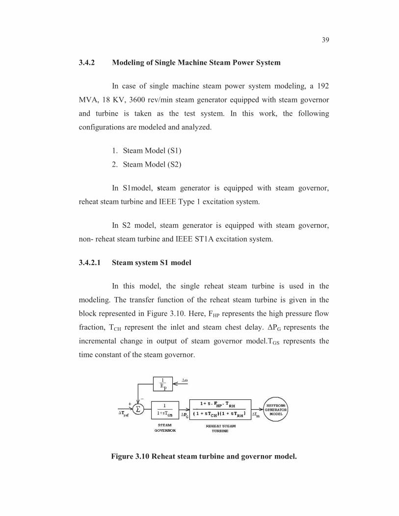
3.4.2 Modeling of Single Machine Steam Power System

In case of single machine steam power system modeling, a 192

MVA, 18 KV, 3600 rev/min steam generator equipped with steam governor

and turbine is taken as the test system. In this work, the following

configurations are modeled and analyzed.

1. Steam Model (S1)

2. Steam Model (S2)

In S1model, steam generator is equipped with steam governor,

reheat steam turbine and IEEE Type 1 excitation system.

In S2 model, steam generator is equipped with steam governor,

non- reheat steam turbine and IEEE ST1A excitation system.

3.4.2.1 Steam system S1 model

In this model, the single reheat steam turbine is used in the

modeling. The transfer function of the reheat steam turbine is given in the

block represented in Figure 3.10. Here, FHP represents the high pressure flow

fraction, TCH represent the inlet and steam chest delay. PG represents the

incremental change in output of steam governor model.TGS represents the

time constant of the steam governor.

Figure 3.10 Reheat steam turbine and governor model.

40

The responses of the reheat turbines are significantly slower than

those that of non-reheat turbines. The main reason is that, the reheater time

constant will have more time delay compared to non-reheat type turbines. The

reheater time constant (TRH) used in this modeling is 6 seconds (IEEE

Standards 2005).This steam system S1 model is equipped with IEEE Type 1

Excitation system.

The state space equation of model (S1) is given by

S1 S1 S1 S1 S1n nx A x B u (3.9)

where n = Number of steam generators, here n=1.

AS1 = State matrix of steam system S1 model.

xS1 and BS1 = State variable vector and input matrix involved.

Equation (3.10) and (3.11) indicate the state variables selected for

this model.

[xS1]OPEN = [ Eq’, EFD VR VE PG Tm]T

(3.10)

[xS1]CLOSED = [ Eq’, EFD VR VE PG Tm, P1 P2 UE]T

(3.11)

3.4.2.2 Steam system S2 model

In this model, the single non-reheat steam turbine has been used in

the modeling. The transfer function of the non-reheat steam turbine is given in

the block given in Figure 3.11. By substituting, the time constant TRH =0 in

the reheat turbine transfer function (Figure 3.10), the transfer function for the

non-reheat turbine has been obtained. Here, the non-reheat time constant is

represented by TTS.

41

Figure 3.11 Non-Reheat Steam turbine and governor model

The state space equation of model (S2) is given by

S2 S2 S2 S2 S2n nx A x B u (3.12)

where n = Number of steam generators, here n=1.

AS2 = State matrix of this steam system model (S2).

XS2 and BS2 = State variable vector and input matrix involved.

Equation (3.13) and (3.14) indicate the state variables selected for

this model.

[xS2]OPEN = [ Eq’, EFD VE PG Tm]T

(3.13)

[xS2]CLOSED = [ Eq’, EFD VE PG Tm, P1 P2 UE]T

(3.14)

42

Table 3.1 Consolidated state variables and state order of hydel and steam

power systems

S.

NoSystem

State variables for various system models

H1

Model

H2

model

S1

model

S2

model

1 Generator , , , ,

2 Excitation

system

Eq’, EFD,

VR VE

Eq’, EFD,

VE

Eq’, EFD,

VR VE

Eq’, EFD,

VE

3 GT Xe, Tm Xe,

Xe’, Tm

PG,

Tm

PG,

Tm

4 PSDC P1 P2,

UE

P1 P2,

UE

P1 P2,

UE

P1 P2,

UE

5 Open loop

State order

8x8 8x8 8x8 7x7

6 Closed loop

State order

11x11 11x11 11x11 10x10

Table 3.1 represents the consolidated view of the various state

variables involved in generator, excitation system, Governor-Turbine and

damping controller of all the models involved in hydel and steam power

systems.

Figure 3.12 represents the complete state space model of the steam

generator equipped with governor-turbine model and PSDC. The state

matrices are developed for all the models involved in both hydel and steam

power systems. The state matrices are given in Appendix 1.

43

Figure 3.12 Complete state space model of steam generator with GT dynamics and PSDC

44

3.5 STATE SPACE MODELING OF MULTIMACHINE HYDEL

AND STEAM POWER SYSTEMS

In this work, three machine nine bus power system model

(Figure 3.2) is taken as the test system for modeling, simulation and analysis.

The single machine Heffron-Phillips generator model (Figure 3.3) is extended

to perform the modeling of multimachine system. Because of the interaction

among various generators in the multimachine system, the branches and loops

of the single machine generator model become multiplied.

For instance, the constant K1 in the single machine model becomes

K1ij,i=1,2…n; j=1,2….n in the multimachine modeling. In this work, n will be

equal to 3, representing the number of generators in the multimachine system

considered. Similarly all the K constants (K1 to K6), damping factor D,inertia

M and the state variables used in the single machine model are generalized for

n-machine notation. Figure 3.13 represents the state space model of

multimachine power system.

Figure 3.13 State space model of multimachine power system

45

For the linearized state space modeling of three machine nine bus

system, the same state space Equations (3.3, 3.6, 3.9 and 3.12) used for

various single machine hydel and steam configurations are implemented for

the multimachine system modeling.

3.6 SUMMARY

In this chapter, a detailed mathematical state space modeling of all

the configurations involved in both single machine and multimachine hydel

and steam power systems considering the effect of governor and turbine

dynamics has been presented. Also, the modeling of damping controller has

been presented. These various hydel and steam power system models form the

basis for all the simulation experiments carried out in this work.