Chapter  2  –  Loads  on  Structures    

�Our  objective  is  to  design  a  structure  that  will  be  able  to  withstand  all  the  loads  to  which  it  is  subjected  while  serving  its  intended  purpose  through  its  intended  life  span.    To  do  so,  �we  must  consider  all  loads  that  can  realistically  be  expected  to  act  on  the  structure  during  its  planned  life  span.    Three  classes  of  Loading  

• Dead  Loads  • Live  Loads  • Environmental  Loads  

 2.1  Dead  Loads    Dead  Loads  are  gravity  loads  of  constant  magnitudes  and  fixed  positions  that  act  permanently  on  the  structure    

     

Example  2.1:    The  floor  beam  is  used  to  support  the  6  ft  width  of  a  lightweight  plain  concrete  slab  having  a  thickness  of  4  in.    The  slab  serves  as  a  portion  of  the  ceiling  for  the  floor  below  and  its  bottom  is  coated  with  plaster.    Furthermore,  an  8  ft  high,  12  in  thick  lightweight  solid  concrete  block  wall  is  directly  over  the  top  flange  of  the  beam.    Determine  the  loading  on  the  beam  measured  per  foot  of  length  of  the  beam  

 

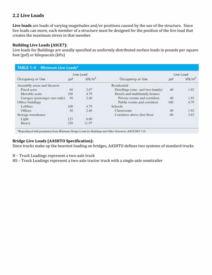
2.2  Live  Loads    Live  loads  are  loads  of  varying  magnitudes  and/or  positions  caused  by  the  use  of  the  structure.    Since  live  loads  can  move,  each  member  of  a  structure  must  be  designed  for  the  position  of  the  live  load  that  creates  the  maximum  stress  in  that  member.    Building  Live  Loads  (ASCE7):  Live  loads  for  Buildings  are  usually  specified  as  uniformly  distributed  surface  loads  in  pounds  per  square  foot  (psf)  or  kilopascals  (kPa)    

   Bridge  Live  Loads  (AASHTO  Specification):  Since  trucks  make  up  the  heaviest  loading  on  bridges,  AASHTO  defines  two  systems  of  standard  trucks    H  –  Truck  Loadings  represent  a  two-­‐axle  truck  HS  –  Truck  Loadings  represent  a  two-­‐axle  tractor  truck  with  a  single-­‐axle  semitrailer    

   

Railroad  Live  Loads  (AREMA  Manual  for  Railway  Engineering):    

   

2.3  Impact    When  live  loads  are  applied  rapidly  to  a  structure  they  cause  larger  stresses  than  those  that  would  be  produced  if  the  same  loads  had  been  applied  gradually.    To  account  for  the  increase  in  stress  due  to  impact,  the  live  loads  expected  to  cause  a  dynamic  effect  on  structures  are  increased  by  certain  impact  percentages  or  impact  factors.    2.4  Wind  Loads  

 Wind  loads  are  produced  by  the  flow  of  wind  around  the  structure.        The  Magnitude  of  wind  loads  depend  on      

Geographical  Location     Nearby  Obstructions   Geometry  and  Vibrational  Characteristics  of  the  Structure  

 ASCE  7  –  05  Determination  of  wind  loads:    

qz  =  0.00256KzKztKdV2I    

where  • qz  =  velocity  pressure  at  height  z  (psf)  • V  =  the  velocity  in  mph  of  a  3  second  gust  of  wind  measured  33  ft  above  the  ground.    Specific  

values  depend  upon  the  category  of  the  structure  obtained  from  a  wind  map.    For  example,  the  interior  portion  of  the  continental  US  reports  a  wind  speed  of  105  mph  if  the  structure  is  an  agricultural  or  storage  building,  since  it  is  of  low  risk  to  human  life  in  the  event  of  a  failure.    The  wind  speed  is  120  mph  for  cases  where  the  structure  is  a  hospital,  since  its  failure  would  cause  substantial  loss  of  human  life.  

• Kz  =  the  velocity  pressure  exposure  coefficient,  which  is  a  function  of  height  and  depends  upon  the  ground  terrain.    Table  1-­‐5  lists  values  for  a  structure  which  is  located  in  open  terrain  with  scattered  low-­‐lying  obstructions  

• Kzt  =  a  factor  that  accounts  for  wind  speed  increases  due  to  hills  and  escarpments.    For  flat  ground  Kzt  =  1.0  

• Kd  =  a  factor  that  accounts  for  the  direction  of  the  wind.    It  is  used  only  when  the  structure  is  subjected  to  a  combination  of  loads.    For  wind  acting  along,  Kd  =  1.0  

 qz  =  Velocity  pressure  at  height  z  (psf)  

Kz  =  velocity  pressure  exposure  coefficient  Kzt  =  Topographic  factor  

Kd  =  Wind  directionality  factor  V  =  wind  speed  (open  terrain  33  ft  above  ground  level)  

I  =  Importance  factor    

   

   

Design  Wind  Pressure  for  Enclosed  Buildings  of  any  height:    

€

p = qGCp − qh GCpi( )    

Where  • q  =  qz  for  the  windward  wall  at  height  z  above  the  ground,  and  q  =  qh  for  the  leeward  walls,  side  

walls,  and  roof,  where  z  =  h,  the  mean  height  of  the  roof  • G  =  a  wind-­‐gust  effect  factor,  which  depends  upon  the  exposure.    For  example,  for  a  rigid  structure,  

G    =  0.85  • Cp  =  a  wall  or  roof  pressure  coefficient  determined  from  a  table  • (GCpi)  =  the  internal  pressure  coefficient,  which  depends  upon  the  type  of  openings  in  the  building.    

For  fully  enclosed  buildings  (GCpi)  =  ±0.18.    Here  signs  indicate  that  either  positive  or  negative  (suction)  pressure  can  occur  within  the  building  

 

   

Example  2.2:    The  enclosed  building  shown  is  used  for  storage  purposes  and  is  located  outside  of  Chicago  Illinois  on  open  flat  terrain.    When  the  wind  is  directed  as  shown  determine  the  design  wind  pressure  acting  on  the  roof  and  sides  of  the  building  using  the  ASCE  7-­‐  10  Specifications.    

 

2.5  Snow  Loads    Design  Loadings  depend  upon  

• Building  shape  • Roof  geometry  • Wind  exposure  • Location  • Importance  • Whether  or  not  its  heated  

 In  the  case  of  a  flat  roof  (slope  <  5%)  the  pressure  loading  can  be  obtained  by  the  following  equation    

€

pf = 0.7CeCtIspg    

• pg  =  ground  snow  loading  • Ce  =  an  exposure  factor  which  depends  upon  the  terrain.    A  fully  exposed  roof  in  an  unobstructed  

area,  Ce  =  0.8,  whereas  a  sheltered  roof  located  in  the  center  of  a  large  city,  Ce  =  1.2  • Ct  =  a  thermal  factor  which  refers  to  the  average  temperature  within  the  building.    For  unheated  

structures  kept  below  freezing  Ct  =  1.2,  whereas  if  the  roof  is  supporting  a  normally  heated  structure,  Ct  =  1.0  

• Is  =  the  importance  factor  as  it  relates  to  occupancy.    For  example  Is  =  0.80  for  agriculture  and  storage  facilities  and  Is  =  1.20  for  schools  and  hospitals  

If  pg  ≤  20psf  then  use  the  larger  value  for  pf,  either  computed  from  the  above  equation  or  from  pf  =  Ispg.    If  pg  >  20psf  ,  then  use  pf  =  Is  (20psf)  

Example  2.3:    The  unheated  storage  facility  shown  is  located  on  flat  open  terrain  in  southern  Illinois,  where  the  specified  ground  snow  load  is  15  psf.    Determine  the  design  snow  load  on  the  roof  which  has  a  slope  of  4%    

 

2.6  Earthquake  Loads    During  an  earthquake  the  foundation  of  the  structure  moves  with  the  ground,  the  above  ground  portion  of  the  structure  resists  the  motion  causing  the  structure  to  vibrate  in  the  horizontal  direction.    These  vibrations  create  horizontal  shear  forces  in  the  structure.    For  an  accurate  prediction  of  the  stresses  a  dynamic  analysis  must  be  performed;  however,  for  low  to  medium  height  buildings,  a  static  analysis  can  be  performed.    The  dynamic  loads  are  approximated  by  a  set  of  static  forces  that  are  applied  laterally  to  the  structure.    

€

V = CsW  • V  =  total  lateral  force  or  base  shear  • Cs  =  seismic  response  coefficient  • W  =  dead  load  of  the  structure  

 

€

Cs =SDSR /IE

 

• Cs  =  the  spectral  response  acceleration  for  short  periods  of  vibration  • R  =  a  response  modification  factor  that  depends  upon  the  ductilityof  the  structure.    Steel  frame  

members  which  are  highly  ductile  can  have  a  value  as  high  as  8,  whereas  reinforced  concrete  frames  can  have  a  value  as  low  as  3.  

• Ie  =  the  importance  factor  that  depends  upon  the  use  of  the  building.    For  example,  I3  =  1  for  agriculture  and  storage  facilities  and  Ie  =  1.5  for  hospitals  and  other  essential  facilities  

 2.7  Hydrostatic  and  Soil  Pressures    Structures  used  to  retain  water  must  be  designed  to  resist  hydrostatic  pressure.    Underground  structures  must  be  designed  to  resist  soil  pressure.    Soil  pressure  consists  of  both  a  vertical  (weight  of  the  soil)  and  horizontal  component.    The  horizontal  component  is  much  less  then  the  vertical  component.    When  portions  of  the  structure  sit  below  the  water  table,  they  must  be  designed  to  counter  act  the  combined  effect  of  hydrostatic  pressure  and  soil  pressure.    2.8  Thermal  and  Other  Effects    Other  effects  such  as  temperature  changes,  blasts,  shrinkage  of  material,  fabrication  errors,  and  differential  settlements  of  supports  may  also  induce  stresses  in  the  structure.    Although  they  are  not  addressed  in  most  building  codes  in  cases  where  they  involve  significant  stresses  they  should  be  considered  in  design.    2.9  Load  Combinations    Probable  combinations  of  loads  must  be  considered  in  design.    To  do  so  ASCE  7  recommends  certain  load  combinations  depending  upon  the  type  of  structural  design  being  used.    ASD  (Allowable-­‐  stress  design)  Allowable  stress  design  combines  material  and  load  uncertainties  into  a  single  factor  of  safety.      Typical  load  combinations  include  

• dead  load  • 0.6(dead  load)  +  0.6(wind  load)  • 0.6(dead  load)  +  0.7(earthquake  load)  

 

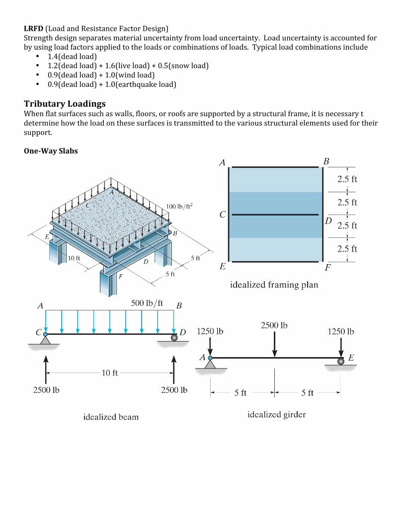
LRFD  (Load  and  Resistance  Factor  Design)  Strength  design  separates  material  uncertainty  from  load  uncertainty.    Load  uncertainty  is  accounted  for  by  using  load  factors  applied  to  the  loads  or  combinations  of  loads.    Typical  load  combinations  include  

• 1.4(dead  load)  • 1.2(dead  load)  +  1.6(live  load)  +  0.5(snow  load)  • 0.9(dead  load)  +  1.0(wind  load)  • 0.9(dead  load)  +  1.0(earthquake  load)  

 Tributary  Loadings  When  flat  surfaces  such  as  walls,  floors,  or  roofs  are  supported  by  a  structural  frame,  it  is  necessary  t  determine  how  the  load  on  these  surfaces  is  transmitted  to  the  various  structural  elements  used  for  their  support.    One-­Way  Slabs  

   

Other  types  of  systems  may  also  be  considered  one-­‐way.    For  the  following  floor  system:      

   

According  to  the  ACI  318  code,  if  L2  >  L1  and  if  the  span  ratio  (L2/L1)  >  2,  the  slab  will  behave  as  a  one-­‐way  slab.    Two-­Way  Slabs    

 

When  working  with  a  two-­‐way  slab  that  is  not  square  our  beams  and  girders  will  have  trapezoidal  and  triangular  distributed  loading.  

 

Example  2.4:    The  floor  of  a  classroom  is  to  be  supported  by  the  bar  joists  shown.    Each  joist  is  15  ft  long  and  they  are  spaced  2.5  ft  on  centers.    The  floor  itself  is  to  be  made  from  lightweight  concrete  that  is  4  in.  thick.    Neglect  the  weight  of  the  joists  and  the  corrugated  metal  deck  and  determine  the  load  that  acts  along  each  joist.  

 

Example  2.5:    The  concrete  girders  of  the  parking  garage  shown  span  30  ft  and  are  15  ft  on  center.    If  the  floor  slab  is  5  in.  thick  and  made  of  reinforced  stone  concrete  and  the  specified  live  load  is  50  psf,  determine  the  distributed  load  the  floor  system  transmits  to  each  interior  girder.