Chapter2 Basics in Conformal Field Theory - Semantic … · 6 2 Basics in Conformal Field Theory Fig. 2.1 Conformal transformation in two dimensions ... symmetric part b ... translation

Chapter 2Basics in Conformal Field Theory

The approach for studying conformal field theories is somewhat different from theusual approach for quantum field theories. Because, instead of starting with a clas-sical action for the fields and quantising them via the canonical quantisation or thepath integral method, one employs the symmetries of the theory. In the spirit ofthe so-called boot-strap approach, for CFTs one defines and for certain cases evensolves the theory just by exploiting the consequences of the symmetries. Such a pro-cedure is possible in two dimensions because the algebra of infinitesimal conformaltransformations in this case is very special: it is infinite dimensional.

In this chapter, we will introduce the basic notions of two-dimensional conformalfield theory from a rather abstract point of view. However, in Sect. 2.9, we will studyin detail three simple examples important for string theory which are given by aLagrangian action.

2.1 The Conformal Group

We start by introducing conformal transformations and determining the conditionfor conformal invariance. Next, we are going to consider flat space in d ≥ 3 di-mensions and identify the conformal group. Finally, we study in detail the caseof Euclidean two-dimensional flat space R

2,0 and determine the conformal groupand the algebra of infinitesimal conformal transformations. We also comment ontwo-dimensional Minkowski space R

1,1 in the end.

2.1.1 Conformal Invariance

Conformal Transformations

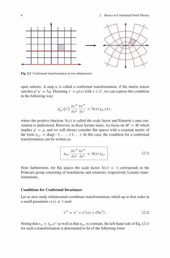
Let us consider a flat space in d dimensions and transformations thereof which lo-cally preserve the angle between any two lines. Such transformations are illustratedin Fig. 2.1 and are called conformal transformations.

In more mathematical terms, a conformal transformation is defined as follows.Let us consider differentiable maps ϕ : U → V , where U ⊂ M and V ⊂ M ′ are

Blumenhagen, R., Plauschinn, E.: Basics in Conformal Field Theory. Lect. Notes Phys. 779, 5–86(2009)DOI 10.1007/978-3-642-00450-6 2 c© Springer-Verlag Berlin Heidelberg 2009

6 2 Basics in Conformal Field Theory

Fig. 2.1 Conformal transformation in two dimensions

open subsets. A map ϕ is called a conformal transformation, if the metric tensorsatisfies ϕ∗g′ = �g. Denoting x ′ = ϕ(x) with x ∈ U , we can express this conditionin the following way:

g′ρσ

(

x ′) �x ′ρ

�xμ

�x ′σ

�xν= �(x) gμν(x) ,

where the positive function �(x) is called the scale factor and Einstein’s sum con-vention is understood. However, in these lecture notes, we focus on M ′ = M whichimplies g′ = g, and we will always consider flat spaces with a constant metric ofthe form ημν = diag(−1, . . . ,+1, . . .). In this case, the condition for a conformaltransformation can be written as

ηρσ

�x ′ρ

�xμ

�x ′σ

�xν= �(x) ημν . (2.1)

Note furthermore, for flat spaces the scale factor �(x) = 1 corresponds to thePoincare group consisting of translations and rotations, respectively Lorentz trans-formations.

Conditions for Conformal Invariance

Let us next study infinitesimal coordinate transformations which up to first order ina small parameter ε(x) � 1 read

x ′ρ = xρ + ερ(x) + O(ε2) . (2.2)

Noting that εμ = ημνεν as well as that ημν is constant, the left-hand side of Eq. (2.1)

for such a transformation is determined to be of the following form:

2.1 The Conformal Group 7

ηρσ

�x ′ρ

�xμ

�x ′σ

�xν= ηρσ

(

δρμ + �ερ

�xμ+ O(ε2)

)(

δσν + �εσ

�xν+ O(ε2)

)

= ημν + ημσ

�εσ

�xν+ ηρν

�ερ

�xμ+ O(ε2)

= ημν +(

�εμ

�xν+ �εν

�xμ

)

+ O(ε2) .

The question we want to ask now is, under what conditions is the transformation(2.2) conformal, i.e. when is Eq. (2.1) satisfied? Introducing the short-hand notation

��xμ = �μ, from the last formula we see that, up to first order in ε, we have to demandthat

�μεν + �νεμ = K (x) ημν ,

where K (x) is some function. This function can be determined by tracing the equa-tion above with ημν

ημν(

�μεν + �νεμ

)

= K (x) ημνημν

2 �μεμ = K (x) d .

Using this expression and solving for K (x), we find the following restriction on thetransformation (2.2) to be conformal:

�μεν + �νεμ = 2

d

(

� · ε)

ημν , (2.3)

where we employed the notation �μεμ = � · ε. Finally, the scale factor can be readoff as �(x) = 1 + 2

d (� · ε) + O(ε2).

Some Useful Relations

Let us now derive two useful equations for later purpose. First, we modify Eq. (2.3)by taking the derivative �ν and summing over ν. We then obtain

�ν(

�μεν + �νεμ

)

= 2

d�ν(

� · ε)

ημν

�μ

(

� · ε) + � εμ = 2

d�μ

(

� · ε)

with � = �μ�μ. Furthermore, we take the derivative �ν to find

�μ�ν

(

� · ε) + � �νεμ = 2

d�μ�ν

(

� · ε)

. (2.4)


After interchanging μ ↔ ν, adding the resulting expression to Eq. (2.4) and usingEq. (2.3) we get

2 �μ�ν

(

� · ε) + �

(

2

d

(

� · ε)

ημν

)

= 4

d�μ�ν

(

� · ε)

,

⇒(

ημν � + (d − 2) �μ�ν

)

(� · ε) = 0 .

Finally, contracting this equation with ημν gives

(d − 1) � (� · ε) = 0 . (2.5)

The second expression we want to use later is obtained by taking derivatives �ρ

of Eq. (2.3) and permuting indices

�ρ�μεν + �ρ�νεμ = 2

dημν �ρ(� · ε) ,

�ν�ρεμ + �μ�ρεν = 2

dηρμ �ν(� · ε) ,

�μ�νερ + �ν�μερ = 2

dηνρ �μ(� · ε) .

Subtracting then the first line from the sum of the last two leads to

2 �μ�νερ = 2

d

(−ημν�ρ + ηρμ�ν + ηνρ�μ

)(

� · ε)

. (2.6)

2.1.2 Conformal Group in d ≥ 3

After having obtained the condition for an infinitesimal transformations to be con-formal, let us now determine the conformal group in the case of dimension d ≥ 3.

Conformal Transformations and Generators

We note that Eq. (2.5) implies that (�·ε) is at most linear in xμ, i.e. (�·ε) = A+Bμxμ

with A and Bμ constant. Then it follows that εμ is at most quadratic in xν and so wecan make the ansatz:

εμ = aμ + bμνxν + cμνρ xνxρ , (2.7)

where aμ, bμν, cμνρ � 1 are constants and the latter is symmetric in the last twoindices, i.e. cμνρ = cμρν . We now study the various terms in Eq. (2.7) separatelybecause the constraints for conformal invariance have to be independent of theposition xμ.


• The constant term aμ in Eq. (2.7) is not constrained by Eq. (2.3). It describes in-finitesimal translations x ′μ = xμ + aμ, for which the generator is the momentumoperator Pμ = −i�μ.

• In order to study the term of Eq. (2.7) which is linear in x , we insert (2.7) intothe condition (2.3) to find

bνμ + bμν = 2

d

(

ηρσ bσρ

)

ημν .

From this expression, we see that bμν can be split into a symmetric and an anti-symmetric part

bμν = α ημν + mμν ,

where mμν = −mνμ. The symmetric term αημν describes infinitesimal scaletransformations x ′μ = (1 + α) xμ with generator D = −i xμ�μ. The anti-symmetric part mμν corresponds to infinitesimal rotations x ′μ = (δμ

ν + mμν) xν

with generator being the angular momentum operator Lμν = i(xμ�ν − xν�μ).• The term of Eq. (2.7) at quadratic order in x can be studied by inserting Eq. (2.7)

into expression (2.6). We then calculate

� · ε = bμμ + 2 cμ

μρ xρ ⇒ �ν

(

� · ε) = 2 cμ

μν ,

from which we find that

cμνρ = ημρbν + ημνbρ − ηνρbμ with bμ = 1

dcρ

ρμ .

The resulting transformations are called Special Conformal Transformations(SCT) and have the following infinitesimal form:

x ′μ = xμ + 2(

x · b)

xμ − (

x · x)

bμ . (2.8)

The corresponding generator is written as Kμ = −i(

2 xμ xν�ν − (

x · x)

�μ

)

.

We have now identified the infinitesimal conformal transformations. However, in or-der to determine the conformal group, we will need the finite conformal transforma-tions which are summarised in Table 2.1 together with the corresponding generators.

Focus on Special Conformal Transformations

For the finite Special Conformal Transformation shown in Table 2.1, one can checkthat expression (2.8) is its infinitesimal version by expanding the denominator forsmall bμ. Furthermore, the scale factor for SCTs is computed as

�(x) =(

1 − 2 (b · x) + (b · b)(x · x))2

.


Table 2.1 Finite conformal transformations and corresponding generators

Transformations Generators

translation x ′μ = xμ + aμ Pμ = −i �μ

dilation x ′μ = α xμ D = −i xμ�μ

rotation x ′μ = Mμν xν Lμν = i

(

xμ�ν − xν�μ

)

SCT x ′μ = xμ−(x ·x)bμ

1−2(b·x)+(b·b)(x ·x) Kμ = −i(

2xμxν�ν − (x · x)�μ

)

Let us also note that for finite Special Conformal Transformations, we can re-writethe expression in Table 2.1 as follows:

x ′μ

x ′ · x ′ = xμ

x · x− bμ .

From this relation, we see that the SCTs can be understood as an inversion of xμ,followed by a translation bμ, and followed again by an inversion. An illustration intwo dimensions is shown in Fig. 2.2.

Finally, we observe that the finite Special Conformal Transformations given inTable 2.1 are not globally defined. In particular, for a given non-zero vector bμ, thereis a point xμ = 1

b·b bμ such that

1 − 2 (b · x) + (b · b)(x · x) = 0 .

Taking into account also the numerator, one finds that xμ is mapped to infinity whichdoes not belong to R

d,0 or Rd−1,1. Therefore, in order to define the finite conformal

transformations globally, one considers the so-called conformal compactificationsof R

d,0 or Rd−1,1, where additional points are included such that the conformal

xµ

xµ

x · x

x′µ

x′µ

x′ · x′−bµ

− 1+1

Fig. 2.2 Illustration of a finite Special Conformal Transformation


transformations are globally defined. We will not go into further detail here, butcome back to this issue in Sect. 2.1.3.

The Conformal Group and Algebra

Before we identify the conformal group and the conformal algebra for the case ofdimensions d ≥ 3, let us first define these objects and point out a subtle difference.

Definition 1. The conformal group is the group consisting of globally defined,invertible and finite conformal transformations (or more concretely, conformal dif-feomorphisms).

Definition 2. The conformal algebra is the Lie algebra corresponding to the con-formal group.

Note that the algebra consisting of generators of infinitesimal conformal transfor-mations contains the conformal algebra as a subalgebra, but it is larger in general.We will encounter an example of this fact in the case of two Euclidean dimensions.

Determining the Conformal Group

Let us finally determine the conformal group for dimensions d ≥ 3. Since the groupis closely related to its algebra, we will concentrate on the later. With the help ofTable 2.1, we can fix the dimension of the algebra by counting the total numberof generators. Keeping in mind that Lμν is anti-symmetric, we find N = d + 1 +d(d−1)

2 + d = (d+2)(d+1)2 . Guided by this result, we perform the definitions

J μ,ν = Lμν , J−1,μ = 12

(

Pμ − Kμ

)

,

J−1,0 = D , J 0,μ = 12

(

Pμ + Kμ

)

.

One can then verify that Jm,n with m, n = −1, 0, 1, . . . , (d−1) satisfy the followingcommutation relations:

[

Jmn, Jrs] = i

(

ηms Jnr + ηnr Jms − ηmr Jns − ηns Jmr)

. (2.9)

For Euclidean d-dimensional space Rd,0, the metric ηmn used above is ηmn =

diag(−1, 1, . . . , 1) and so we identify Eq. (2.9) as the commutation relations ofthe Lie algebra so(d + 1, 1). Similarly, in the case of R

d−1,1, the metric is ηmn =diag(−1,−1, 1, . . . , 1) for which Eq. (2.9) are the commutation relations of the Liealgebra so(d, 2). These two examples are illustrations of the general result that

For the case of dimensions d = p + q ≥ 3, the conformal group of Rp,q

is SO(p + 1, q + 1).


2.1.3 Conformal Group in d = 2

Let us now study the conformal group for the special case of two dimensions. Wewill work with an Euclidean metric in a flat space but address the case of Lorentziansignature in the end.

Conformal Transformations

The condition (2.3) for invariance under infinitesimal conformal transformations intwo dimensions reads as follows:

�0 ε0 = +�1 ε1 , �0 ε1 = −�1 ε0 , (2.10)

which we recognise as the familiar Cauchy–Riemann equations appearing in com-plex analysis. A complex function whose real and imaginary parts satisfy Eq. (2.10)is a holomorphic function (in some open set). We then introduce complex variablesin the following way:

z = x0 + i x1 , ε = ε0 + iε1 , �z = 12

(

�0 − i�1)

,

z = x0 − i x1 , ε = ε0 − iε1 �z = 12

(

�0 + i�1)

.

Since ε(z) is holomorphic, so is f (z) = z + ε(z) from which we conclude that

A holomorphic function f (z) = z + ε(z) gives rise to an infinitesimaltwo-dimensional conformal transformation z �→ f (z).

This implies that the metric tensor transforms under z �→ f (z) as follows:

ds2 = dz dz �→ � f

�z

� f

�zdz dz ,

from which we infer the scale factor as∣

∣� f�z

∣

∣

2.

The Witt Algebra

As we have observed above, for an infinitesimal conformal transformation in twodimensions the function ε(z) has to be holomorphic in some open set. However, it isreasonable to assume that ε(z) in general is a meromorphic function having isolatedsingularities outside this open set. We therefore perform a Laurent expansion ofε(z) around say z = 0. A general infinitesimal conformal transformation can thenbe written as


z′ = z + ε(z) = z +∑

n∈Z

εn(−zn+1

)

,

z′ = z + ε(z) = z +∑

n∈Z

εn(−zn+1) ,

where the infinitesimal parameters εn and εn are constant. The generators corre-sponding to a transformation for a particular n are

ln = −zn+1�z and ln = −zn+1�z . (2.11)

It is important to note that since n ∈ Z, the number of independent infinitesimalconformal transformations is infinite. This observation is special to two dimensionsand we will see that it has far-reaching consequences.

As a next step, let us compute the commutators of the generators (2.11) in orderto determine the corresponding algebra. We calculate

[

lm, ln] = zm+1�z

(

zn+1�z) − zn+1�z

(

zm+1�z)

= (n + 1) zm+n+1�z − (m + 1) zm+n+1�z

= −(m − n) zm+n+1�z

= (m − n) lm+n ,

[

lm, ln] = (m − n) lm+n ,

[

lm, ln] = 0 .

(2.12)

The first commutation relations define one copy of the so-called Witt algebra, andbecause of the other two relations, there is a second copy which commutes with thefirst one. We can then summarise our findings as follows:

The algebra of infinitesimal conformal transformations in an Euclideantwo-dimensional space is infinite dimensional.

Note that, since we can identify two independent copies of the Witt algebra gener-ated by Eq. (2.11), it is customary to treat z and z as independent variables whichmeans that we are effectively considering C

2 instead of C. We will come back tothis point in Sect. 2.2.

Global Conformal Transformations

Let us now focus on the copy of the Witt algebra generated by {ln} and observe thaton the Euclidean plane R

2 � C, the generators ln are not everywhere defined. Inparticular, there is an ambiguity at z = 0 and it turns out to be necessary not to work


on C but on the Riemann sphere S2 � C∪{∞} being the conformal compactificationof R

2.But even on the Riemann sphere, not all of the generators (2.11) are well defined.

For z = 0, we find that

ln = −zn+1�z, non-singular at z = 0 only for n ≥ −1 .

The other ambiguous point is z = ∞ which is, however, part of the Riemann sphereS2. To investigate the behaviour of ln there, let us perform the change of variablez = − 1

wand study w → 0. We then observe that

ln = −(

− 1

w

)n−1

�w, non-singular at w = 0 only for n ≤ +1 ,

where we employed that �z = (−w)2�w. We therefore arrive at the conclusion that

Globally defined conformal transformations on the Riemann sphere S2 =C ∪ ∞ are generated by {l−1, l0, l+1}.

The Conformal Group

After having determined the operators generating global conformal transformations,we will now determine the conformal group.

• As it is clear from its definition, the operator l−1 generates translations z �→ z+b.• For the operator l0, let us recall that l0 = −z �z . Therefore, l0 generates trans-

formations z �→ a z with a ∈ C. In order to get a geometric intuition of suchtransformations, we perform the change of variables z = reiφ to find

l0 = −1

2r�r + i

2�φ , l0 = −1

2r�r − i

2�φ .

Out of those, we can form the linear combinations

l0 + l0 = −r�r and i(

l0 − l0) = −�φ , (2.13)

and so we see that l0 + l0 is the generator for two-dimensional dilations and thati(l0 − l0) is the generator of rotations.

• Finally, the operator l+1 corresponds to Special Conformal Transformationswhich are translations for the variable w = − 1

z . Indeed, c l1z = −c z2 is theinfinitesimal version of the transformations z �→ z

c z+1 which corresponds tow �→ w − c.

In summary, we have argued that the operators {l−1, l0, l+1} generate transforma-tions of the form


z �→ az + b

cz + dwith a, b, c, d ∈ C . (2.14)

For this transformation to be invertible, we have to require that ad − bc is non-zero. If this is the case, we can scale the constants a, b, c, d such that ad − bc =1. Furthermore, note that the expression above is invariant under (a, b, c, d) �→(−a,−b,−c,−d). From the conformal transformations (2.14) together with theserestrictions, we can then infer that

The conformal group of the Riemann sphere S2 = C ∪ ∞ is the Mobiusgroup SL(2, C)/Z2.

Virasoro Algebra

Let us now come back to the Witt algebra of infinitesimal conformal transforma-tions. As it turns out, this algebra admits a so-called central extension. Withoutproviding a mathematically rigorous definition, we state that the central extensiong = g ⊕ C of a Lie algebra g by C is characterised by the commutation relations

[

x, y]

g= [

x, y]

g+ c p(x, y) , x, y ∈ g ,

[

x, c]

g= 0 , x, y ∈ g ,

[

c, c]

g= 0 , c ∈ C ,

where p : g × g → C is bilinear. Central extensions of algebras are closely re-lated to projective representations which are common to Quantum Mechanics. Inthe following, we are going to allow for such additional structure.

More concretely, let us denote the elements of the central extension of the Wittalgebra by Ln with n ∈ Z and write their commutation relations as

[

Lm, Ln] = (m − n) Lm+n + cp(m, n) . (2.15)

Of course, a similar analysis can be carried out for the generators ln ↔ Ln . Theprecise form of p(m, n) is determined in the following way:

• First, from Eq. (2.15) it is clear that p(m, n) = −p(n, m) in order for p(m, n) tobe compatible with the anti-symmetry of the Lie bracket.

• We also observe that one can always arrange for p(1,−1) = 0 and p(n, 0) = 0by a redefinition

Ln = Ln + cp(n, 0)

nfor n �= 0 , L0 = L0 + cp(1,−1)

2.

Indeed, for the modified generators we see that the p(n, m) vanishes


[

Ln,L0] = n Ln + cp(n, 0) = n Ln ,

[

L1,L−1] = 2 L0 + cp(1,−1) = 2L0 .

• Next, we compute the following particular Jacobi identity:

0 = [[

Lm, Ln]

, L0] + [[

Ln, L0]

, Lm] + [[

L0, Lm]

, Ln]

0 = (m − n) cp(m + n, 0) + n cp(n, m) − m cp(m, n)

0 = (m + n) p(n, m)

from which we infer that in the case n �= −m, we have p(n, m) = 0. Therefore,the only non-vanishing central extensions are p(n,−n) for |n| ≥ 2.

• We finally calculate the following Jacobi identity:

0 = [[

L−n+1, Ln]

, L−1] + [[

Ln, L−1]

, L−n+1] + [[

L−1, L−n+1]

, Ln]

0 = (−2n + 1) cp(1,−1) + (n + 1) cp(n − 1,−n + 1) + (n − 2) cp(−n, n)

which leads to a recursion relation of the form

p(n,−n) = n + 1

n − 2p(n − 1,−n + 1) = . . .

= 1

2

(

n + 1

3

)

= 1

12(n + 1)n(n − 1)

where we have normalised p(2,−2) = 12 . This normalisation is chosen such that

the constant c has a particular value for the standard example of the free bosonwhich we will study in Sect. 2.9.1.

The central extension of the Witt algebra is called the Virasoro algebra and theconstant c is called the central charge. In summary,

The Virasoro algebra Virc with central charge c has the commutationrelations

[

Lm, Ln] = (m − n) Lm+n + c

12(m3 − m) δm+n,0 . (2.16)

Remarks

• Without providing a rigorous mathematical definition, we note that above wehave computed the second cohomology group H 2 of the Witt algebra. It is gen-erally true that H 2(g, C) classifies the central extensions of an algebra g moduloredefinitions of the generators. However, for semi-simple finite dimensional Liealgebras, one finds that their second cohomology group vanishes and so in thiscase there do not exist any central extensions.

2.2 Primary Fields 17

• Since p(m, n) = 0 for m, n = −1, 0,+1, it is still true that L−1 generatestranslations, L0 generates dilations and rotations, and that L+1 generates Spe-cial Conformal Transformations. Therefore, also {L−1, L0, L1} are generators ofSL(2, C)/Z2 transformations. This just reflects the above mentioned fact that thefinite-dimensional Lie algebras do not have any non-trivial central extensions.

• By computing ||L−m | 0〉||2 = 〈0 |L+m L−m | 0〉 = c12 (m3 − m), one observes that

only for c �= 0 there exist non-trivial representations of the Virasoro algebra. Wehave not yet provided the necessary techniques to perform this calculation but wewill do so in the rest of this chapter.

• In this section, we have determined the conformal transformations and theconformal algebra for two-dimensional Euclidean space. However, for a two-dimensional flat space–time with Lorentzian signature, one can perform a similaranalysis. To do so, one defines light-cone coordinates u = −t +x and v = +t +xwhere t denotes the time direction and x the space direction. In these variables,we find

ds2 = −dt2 + dx2 = du dv ,

and conformal transformations are given by u �→ f (u) and v �→ g(v) lead-ing to ds ′2 = �u f �vg du dv. Therefore, the algebra of infinitesimal conformaltransformations is again infinite dimensional.

2.2 Primary Fields

In this section, we will establish some basic definitions for two-dimensional confor-mal field theories in Euclidean space.

Complexification

Let us start with an Euclidean two-dimensional space R2 and perform the natural

identification R2 � C by introducing complex variables z = x0 + i x1 and

z = x0 − i x1. From Eq. (2.12), we have seen that we can identify two commutingcopies of the Witt algebra which naturally extend to the Virasoro algebra. Since thegenerators of the Witt algebras are expressed in terms of z and z, it turns out to beconvenient to consider them as two independent complex variables. For the fields φ

of our theory, this complexification R2 → C

2 means

φ(

x0, x1) −→ φ

(

z, z)

,

where {x0, x1} ∈ R2 and {z, z} ∈ C

2. However, note that at some point we have toidentify z with the complex conjugate z∗ of z.


Definition of Chiral and Primary Fields

Definition 3. Fields only depending on z, i.e. φ(z), are called chiral fields and fieldsφ(z) only depending on z are called anti-chiral fields. It is also common to usethe terminology holomorphic and anti-holomorphic in order to distinguish betweenchiral and anti-chiral quantities.

Definition 4. If a field φ(z, z) transforms under scalings z �→ λz according to

φ(

z, z) �→ φ′(z, z

) = λh λhφ(

λ z, λz)

,

it is said to have conformal dimensions (h, h).

Definition 5. If a field transforms under conformal transformations z �→ f (z) ac-cording to

φ(

z, z) �→ φ′(z, z

) =(� f

�z

)h(� f

�z

)hφ(

f (z), f (z))

, (2.17)

it is called a primary field of conformal dimension (h, h). If Eq. (2.17) holds only forf ∈ SL(2, C)/Z2, i.e. only for global conformal transformations, then φ is called aquasi-primary field.

Note that a primary field is always quasi-primary but the reverse is not true.Furthermore, not all fields in a CFT are primary or quasi-primary. Those fields arecalled secondary fields.

Infinitesimal Conformal Transformations of Primary Fields

Let us now investigate how a primary field φ(z, z) behaves under infinitesimalconformal transformations. To do so, we consider the map f (z) = z + ε(z) withε(z) � 1 and compute the following quantities up to first order in ε(z):

(

� f

�z

)h

= 1 + h �zε(z) + O(ε2) ,

φ(

z + ε(z), z) = φ(z) + ε(z) �zφ(z, z) + O(ε2) .

Using these two expressions in the definition of a primary field (2.17), we obtain

φ(z, z) �→ φ(z, z) +(

h �zε + ε�z + h �zε + ε�z

)

φ(z, z) ,

and so the transformation of a primary field under infinitesimal conformal transfor-mations reads

δ ε,ε φ(z, z) =(

h �zε + ε �z + h �zε + ε �z

)

φ(z, z) . (2.18)

2.3 The Energy–Momentum Tensor 19

2.3 The Energy–Momentum Tensor

Usually, a Field Theory is defined in terms of a Lagrangian action from which onecan derive various objects and properties of the theory. In particular, the energy–momentum tensor can be deduced from the variation of the action with respect tothe metric and so it encodes the behaviour of the theory under infinitesimal trans-formations gμν �→ gμν + δgμν with δgμν � 1.

Since the algebra of infinitesimal conformal transformations in two dimensionsis infinite dimensional, there are strong constraints on a conformal field theory. Inparticular, it turns out to be possible to study such a theory without knowing theexplicit form of the action. The only information needed is the behaviour underconformal transformations which is encoded in the energy–momentum tensor.

Implication of Conformal Invariance

In order to study the energy–momentum tensor for CFTs, let us recall Noether’stheorem which states that for every continuous symmetry in a Field Theory, there isa current jμ which is conserved, i.e. �μ jμ = 0. Since we are interested in theorieswith a conformal symmetry xμ �→ xμ + εμ(x), we have a conserved current whichcan be written as

jμ = Tμν εν , (2.19)

where the tensor Tμν is symmetric and is called the energy–momentum tensor. Sincethis current is preserved, we obtain for the special case εμ = const. that

0 = �μ jμ = �μ(

Tμν εν) = (

�μTμν

)

εν ⇒ �μTμν = 0 . (2.20)

For more general transformations εμ(x), the conservation of the current (2.19) im-plies the following relation:

0 = �μ jμ = (

�μTμν

)

εν + Tμν

(

�μεν)

= 0 + 1

2Tμν

(

�μεν + �νεμ) = 1

2Tμνη

μν(

� · ε) 2

d= 1

dTμ

μ(

� · ε)

,

where we used Eq. (2.3) and the fact that Tμν is symmetric. Since this equation hasto be true for arbitrary infinitesimal transformations ε(z), we conclude

In a conformal field theory, the energy–momentum tensor Tμν is trace-less, that is, Tμ

μ = 0.


Specialising to Two Euclidean Dimensions

Let us now investigate the consequences of a traceless energy–momentum tensorfor two-dimensional CFTs in the case of Euclidean signature. To do so, we againperform the change of coordinates from the real to the complex ones shown on p. 12.Using then Tμν = �xα

�xμ�xβ

�xν Tαβ for x0 = 12 (z + z) and x1 = 1

2i (z − z), we find

Tzz = 1

4

(

T00 − 2i T10 − T11)

,

Tzz = 1

4

(

T00 + 2i T10 − T11)

,

Tzz = Tzz = 1

4

(

T00 + T11) = 1

4Tμ

μ = 0 ,

where for Tzz we used that ημν = diag(+1,+1) together with Tμμ = 0. Employing

the latter relation also for the left-hand side, we obtain

Tzz = 1

2

(

T00 − i T10)

, Tzz = 1

2

(

T00 + i T10)

. (2.21)

Using finally the condition for translational invariance (2.20), we find

�0T00 + �1T10 = 0 , �0T01 + �1T11 = 0 , (2.22)

from which it follows that

�zTzz = 1

4

(

�0 + i�1)(

T00 − iT10) = 1

4

(

�0T00 + �1T10 + i�1 T00︸︷︷︸

= −T11

− i�0 T10︸︷︷︸

= T01

) = 0 ,

where we used Eq. (2.22) and Tμμ = 0. Similarly, one can show that �zTzz = 0

which leads us to the conclusion that

The two non-vanishing components of the energy–momentum tensor area chiral and an anti-chiral field

Tzz(z, z) =: T (z) , Tzz(z, z) =: T (z) .

2.4 Radial Quantisation

Motivation and Notation

In the following, we will focus our studies on conformal field theories defined onEuclidean two-dimensional flat space. Although this choice is arbitrary, for con-creteness we denote the Euclidean time direction by x0 and the Euclidean space

2.4 Radial Quantisation 21

direction by x1. Furthermore, note that theories with a Lorentzian signature can beobtained from the Euclidean ones via a Wick rotation x0 → i x0.

Next, we compactify the Euclidean space direction x1 on a circle of radius Rwhich we will mostly choose as R = 1. The CFT we obtain in this way is thus de-fined on a cylinder of infinite length for which we introduce the complex coordinatew defined as

w = x0 + i x1 , w ∼ w + 2π i ,

where we also indicated the periodic identification. Let us emphasise that the theoryon the cylinder is the starting point for our following analysis. This is also natu-ral from a string theory point of view, since the world-sheet of a closed string inEuclidean coordinates is a cylinder.

Mapping the Cylinder to the Complex Plane

After having explained our initial theory, we now introduce the concept of radialquantisation of a two-dimensional Euclidean CFT. To do so, we perform a changeof variables by mapping the cylinder to the complex plane in order to employ thepower of complex analysis. In particular, this mapping is achieved by

z = ew = ex0 · eix1, (2.23)

which is a map from an infinite cylinder described by x0 and x1 to the complexplane described by z (see Fig. 2.3). The former time translations x0 �→ x0 + a arethen mapped to complex dilation z �→ eaz and the space translations x1 �→ x1 + bare mapped to rotations z �→ eibz.

As it is known from Quantum Mechanics, the generator of time translations isthe Hamiltonian which in the present case corresponds to the dilation operator.

x0

x1x0

x1

z

Fig. 2.3 Mapping the cylinder to the complex plane


Similarly, the generator for space translations is the momentum operator corre-sponding to rotations. Recalling Eq. (2.13) together with the observation that thecentral extension for L0 and L0 vanishes, we find that

H = L0 + L0 , P = i(

L0 − L0)

. (2.24)

Asymptotic States

We now consider a field φ(z, z) with conformal dimensions (h, h) for which we canperform a Laurent expansion around z0 = z0 = 0

φ(z, z) =∑

n,m∈Z

z−n−h z−m−h φn,m , (2.25)

where the additional factors of h and h in the exponents can be explained by themap (2.23), but also lead to scaling dimensions (n, m) for φn,m . The quantisation ofthis field is achieved by promoting the Laurent modes φn,m to operators. This pro-cedure can be motivated by considering the theory on the cylinder and performing aFourier expansion of φ(x0, x1). As usual, upon quantisation the Fourier modes areconsidered to be operators which, after mapping to the complex plane, agree withthe approach above.

Next, we note that via Eq. (2.23) the infinite past on the cylinder x0 = −∞ ismapped to z = z = 0. This motivates the definition of an asymptotic in-state |φ〉 tobe of the following form:

∣

∣φ⟩ = lim

z,z→0φ(z, z)

∣

∣0⟩

. (2.26)

However, in order for Eq. (2.26) to be non-singular at z = 0, that is, to be a well-defined asymptotic in-state, we require

φn,m

∣

∣0⟩ = 0 for n > −h, m > −h . (2.27)

Using this restriction together with the mode expansion (2.25), we can simplifyEq. (2.26) in the following way:

∣

∣φ⟩ = lim

z,z→0φ(z, z)

∣

∣0⟩ = φ−h,−h

∣

∣0⟩

. (2.28)

Hermitian Conjugation

In order to obtain the hermitian conjugate φ† of a field φ, we note that in Euclideanspace there is a non-trivial action on the Euclidean time x0 = i t upon hermitianconjugation. Because of the complex conjugation, we find x0 �→ −x0 while theEuclidean space coordinate x1 is left invariant. For the complex coordinate z =

2.5 The Operator Product Expansion 23

exp(x0+i x1), hermitian conjugation thus translates to z �→ 1/z, where we identifiedz with the complex conjugate z∗ of z. We then define the hermitian conjugate of afield φ as

φ†(z, z) = z−2h z−2h φ

(

1

z,

1

z

)

. (2.29)

Performing a Laurent expansion of the hermitian conjugate field φ† gives us thefollowing result:

φ†(z, z) = z−2h z−2h∑

n,m∈Z

z+n+h z+m+h φn,m =∑

n,m∈Z

z+n−h z+m−h φn,m , (2.30)

and if we compare this expression with the hermitian conjugate of Eq. (2.25), wesee that for the Laurent modes we find

(

φn,m)† = φ−n,−m . (2.31)

Let us finally define a relation similar as Eq. (2.26) for an asymptotic out-statesof a CFT. Naturally, this is achieved by using the hermitian conjugate field whichreads

⟨

φ∣

∣ = limz,z→0

⟨

0∣

∣ φ†(z, z) = limw,w→∞

w2h w 2h⟨

0∣

∣ φ(w,w) ,

where we employed Eq. (2.29) together with z = w−1 and z = w−1. However, bythe same reasoning as above, in order for the asymptotic out-state to be well defined,we require

⟨

0∣

∣ φn,m = 0 for n < h, m < h .

Recalling for instance Eq. (2.30), we can then simplify the definition of the out-stateas follows:

⟨

φ∣

∣ = limw,w→∞

w2h w 2h⟨

0∣

∣ φ(w,w) = ⟨

0∣

∣ φ+h,+h . (2.32)

2.5 The Operator Product Expansion

In this section, we will study in more detail the energy–momentum tensor andthereby introduce the operator formalism for two-dimensional conformal field the-ories.


Conserved Charges

To start, let us recall that since the current jμ = Tμνεν associated to the conformal

symmetry is preserved, there exists a conserved charge which is expressed in thefollowing way:

Q =∫

dx1 j0 at x0 = const. . (2.33)

In Field Theory, this conserved charge is the generator of symmetry transformationsfor an operator A which can be written as

δA = [

Q, A]

,

where the commutator is evaluated at equal times. From the change of coordinates(2.23), we infer that x0 = const. corresponds to |z| = const. and so the integralover space

∫

dx1 in Eq. (2.33) gets transformed into a contour integral. With theconvention that contour integrals

∮

dz are always counter clockwise, the naturalgeneralisation of the conserved charge (2.33) to complex coordinates reads

Q = 1

2π i

∮

C

(

dz T (z) ε(z) + dz T (z) ε(z))

. (2.34)

This expression allows us now to determine the infinitesimal transformation of afield φ(z, z) generated by a conserved charge Q. To do so, we compute δφ = [Q, φ]which, using Eq. (2.34), becomes

δ ε,ε φ(w,w) = 1

2π i

∮

Cdz

[

T (z)ε(z), φ(w,w)] + 1

2π i

∮

Cdz

[

T (z)ε(z), φ(w,w)]

.

(2.35)

Radial Ordering

Note that there is some ambiguity in Eq. (2.35) because we have to decide whetherw and w are inside or outside the contour C. However, from quantum field theorywe know that correlation functions are only defined as a time ordered product. Con-sidering the change of coordinates (2.23), in a CFT the time ordering becomes aradial ordering and thus the product A(z)B(w) does only make sense for |z| > |w|.To this end, we define the radial ordering of two operators as

R(

A(z) B(w))

:={

A(z) B(w) for |z| > |w| ,

B(w) A(z) for |w| > |z| .

With this definition, it is clear that we have to interpret an expression such asEq. (2.35) in the following way:


∮

dz[

A(z), B(w)] =

∮

|z|>|w|dz A(z) B(w) −

∮

|z|<|w|dz B(w) A(z)

=∮

C(w)dz R

(

A(z) B(w))

,

(2.36)

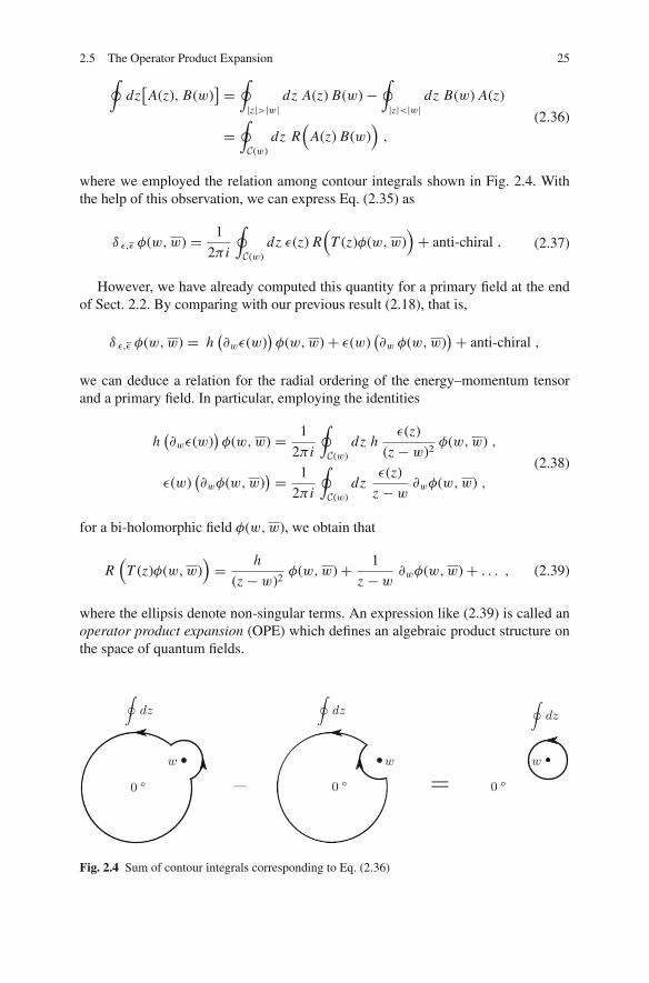
where we employed the relation among contour integrals shown in Fig. 2.4. Withthe help of this observation, we can express Eq. (2.35) as

δ ε,ε φ(w,w) = 1

2π i

∮

C(w)dz ε(z) R

(

T (z)φ(w,w))

+ anti-chiral . (2.37)

However, we have already computed this quantity for a primary field at the endof Sect. 2.2. By comparing with our previous result (2.18), that is,

δ ε,ε φ(w,w) = h(

�wε(w))

φ(w,w) + ε(w)(

�w φ(w,w)) + anti-chiral ,

we can deduce a relation for the radial ordering of the energy–momentum tensorand a primary field. In particular, employing the identities

h(

�wε(w))

φ(w,w) = 1

2π i

∮

C(w)dz h

ε(z)

(z − w)2φ(w,w) ,

ε(w)(

�wφ(w,w)) = 1

2π i

∮

C(w)dz

ε(z)

z − w�wφ(w,w) ,

(2.38)

for a bi-holomorphic field φ(w,w), we obtain that

R(

T (z)φ(w,w))

= h

(z − w)2φ(w,w) + 1

z − w�wφ(w,w) + . . . , (2.39)

where the ellipsis denote non-singular terms. An expression like (2.39) is called anoperator product expansion (OPE) which defines an algebraic product structure onthe space of quantum fields.

∮dz

∮dz

∮dz

www

0 ° 0 ° 0 °– =

Fig. 2.4 Sum of contour integrals corresponding to Eq. (2.36)


To ease our notation, in the following, we will always assume radial ordering fora product of fields, i.e. we write A(z)B(w) instead of R(A(z)B(w)). Furthermore,with the help of Eq. (2.39) we can give an alternative definition of a primary field:

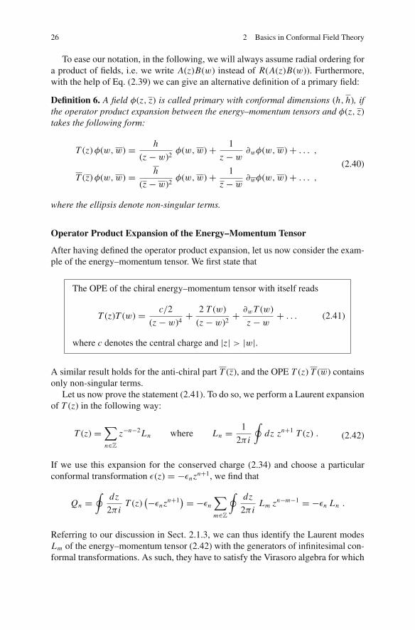
Definition 6. A field φ(z, z) is called primary with conformal dimensions (h, h), ifthe operator product expansion between the energy–momentum tensors and φ(z, z)takes the following form:

T (z) φ(w,w) = h

(z − w)2φ(w,w) + 1

z − w�wφ(w,w) + . . . ,

T (z) φ(w,w) = h

(z − w)2φ(w,w) + 1

z − w�wφ(w,w) + . . . ,

(2.40)

where the ellipsis denote non-singular terms.

Operator Product Expansion of the Energy–Momentum Tensor

After having defined the operator product expansion, let us now consider the exam-ple of the energy–momentum tensor. We first state that

The OPE of the chiral energy–momentum tensor with itself reads

T (z)T (w) = c/2

(z − w)4+ 2 T (w)

(z − w)2+ �wT (w)

z − w+ . . . (2.41)

where c denotes the central charge and |z| > |w|.

A similar result holds for the anti-chiral part T (z), and the OPE T (z) T (w) containsonly non-singular terms.

Let us now prove the statement (2.41). To do so, we perform a Laurent expansionof T (z) in the following way:

T (z) =∑

n∈Z

z−n−2Ln where Ln = 1

2π i

∮

dz zn+1 T (z) . (2.42)

If we use this expansion for the conserved charge (2.34) and choose a particularconformal transformation ε(z) = −εnzn+1, we find that

Qn =∮

dz

2π iT (z)

(−εnzn+1) = −εn

∑

m∈Z

∮

dz

2π iLm zn−m−1 = −εn Ln .

Referring to our discussion in Sect. 2.1.3, we can thus identify the Laurent modesLm of the energy–momentum tensor (2.42) with the generators of infinitesimal con-formal transformations. As such, they have to satisfy the Virasoro algebra for which


we calculate

[

Lm, Ln] =

∮

dz

2π i

∮

dw

2π izm+1 wn+1

[

T (z), T (w)]

=∮

C(0)

dw

2π iwn+1

∮

C(w)

dz

2π izm+1 R

(

T (z)T (w))

=∮

C(0)

dw

2π iwn+1

∮

C(w)

dz

2π izm+1

(

c/2

(z − w)4+ 2 T (w)

(z − w)2+ �wT (w)

z − w

)

=∮

C(0)

dw

2π iwn+1

(

(m + 1)m(m − 1) wm−2 c

2 · 3!

+ 2 (m + 1) wm T (w) + wm+1�wT (w))

=∮

dw

2π i

(

c

12

(

m3 − m)

wm+n−1

+ 2 (m + 1) wm+n+1 T (w) + wm+n+2 �wT (w)

)

= c

12

(

m3 − m)

δm,−n + 2 (m + 1) Lm+n

+ 0 −∮

dw

2π i(m + n + 2) T (w) wm+n+1

︸︷︷︸

= (m + n + 2) Lm+n

= (m − n) Lm+n + c

12

(

m3 − m)

δm,−n ,

where we performed an integration by parts to evaluate the �wT (w) term. Therefore,we have shown that Eq. (2.41) is the correct form of the OPE between two energy–momentum tensors.

Conformal Transformations of the Energy–Momentum Tensor

To end this section, we will investigate the behaviour of the energy–momentumtensor under conformal transformations. In particular, by comparing the OPE (2.41)with the definition (2.40), we see that for non-vanishing central charges, T (z) is nota primary field. But, one can show that under conformal transformations f (z), theenergy–momentum tensor behaves as

T ′(z) =

(

� f

�z

)2

T(

f (z)) + c

12S(

f (z), z)

, (2.43)

where S(w, z) denotes the Schwarzian derivative


S(w, z) = 1

(�zw)2

(

(

�zw)(

�3zw

) − 3

2

(

�2zw

)2)

.

We will not prove Eq. (2.43) in detail but verify it on the level of infinitesimalconformal transformations f (z) = z +ε(z). In order to do so, we first use Eq. (2.37)with the OPE of the energy–momentum tensor (2.41) to find

δ ε T (z) = 1

2π i

∮

C(z)dw ε(w) T (w) T (z)

= 1

2π i

∮

C(z)dw ε(w)

(

c/2

(w − z)4+ 2 T (z)

(w − z)2+ �z T (z)

w − z+ . . .

)

= c

12�3

zε(z) + 2 T (z) �zε(z) + ε(z) �zT (z) . (2.44)

Let us compare this expression with Eq. (2.43). For infinitesimal transformationsf (z) = z + ε(z), the leading order contribution to the Schwarzian derivative reads

S(

z + ε(z), z) = 1

(1 + �zε)2

(

(

1 + �zε)

�3zε − 3

2

(

�2zε)2)

� �3zε(z) .

The variation of the energy–momentum tensor can then be computed as

δ ε T (z) = T ′(z) − T (z)

=(

1 + �zε(z))2(

T (z) + ε(z) �zT (z))

+ c

12�3

zε(z) − T (z)

= c

12�3

zε(z) + 2 T (z) �zε(z) + ε(z) �zT (z) ,

which is the same as in Eq. (2.44). We have thus verified Eq. (2.43) at the level ofinfinitesimal conformal transformations.

Remarks

• The calculation on p. 27 shows that the singular part of the OPE of the chiralenergy–momentum tensors T (z) is equivalent to the Virasoro algebra for themodes Lm .

• Performing a computation along the same lines as on p. 27, one finds that for achiral primary field φ(z), the holomorphic part of the OPE (2.40) is equivalent to

[

Lm, φn] = (

(h − 1)m − n)

φm+n (2.45)

for all m, n ∈ Z. If relations (2.40) and (2.45) hold only for m = −1, 0,+1, thenφ(z) is called a quasi-primary field.

2.6 Operator Algebra of Chiral Quasi-Primary Fields 29

• Applying the relation (2.45) to the Virasoro algebra (2.16) for valuesm = −1, 0,+1, we see that the chiral energy–momentum tensor is a quasi-primary field of conformal dimension (h, h) = (2, 0). In view of Eq. (2.25), thisobservation also explains the form of the Laurent expansion (2.42).

• It is worth to note that the Schwarzian derivative S(w, z) vanishes for SL(2, C)transformations w = f (z) in agreement with the fact that T (z) is a quasi-primaryfield.

2.6 Operator Algebra of Chiral Quasi-Primary Fields

The objects of interest in quantum field theories are n-point correlation functionswhich are usually computed in a perturbative approach via either canonical quan-tisation or the path integral method. In this section, we will see that the exact two-and three-point functions for certain fields in a conformal field theory are alreadydetermined by the symmetries. This will allow us to derive a general formula for theOPE among quasi-primary fields.

2.6.1 Conformal Ward Identity

In quantum field theory, so-called Ward identities are the quantum manifestation ofsymmetries. We will now derive such an identity for the conformal symmetry oftwo-dimensional CFTs on general grounds. For primary fields φi , we calculate

⟨

∮

dz

2π iε(z) T (z) φ1(w1, w1) . . . φN (wN , wN )

⟩

(2.46)

=N∑

i=1

⟨

φ1(w1, w1) . . .(

∮

C(wi )

dz

2π iε(z) T (z) φi (wi , wi )

)

. . . φN (wN , wN )⟩

=N∑

i=1

⟨

φ1(w1, w1) . . .(

hi �ε(wi ) + ε(wi ) �wi

)

φi (wi , wi ) . . . φN (wN , wN )⟩

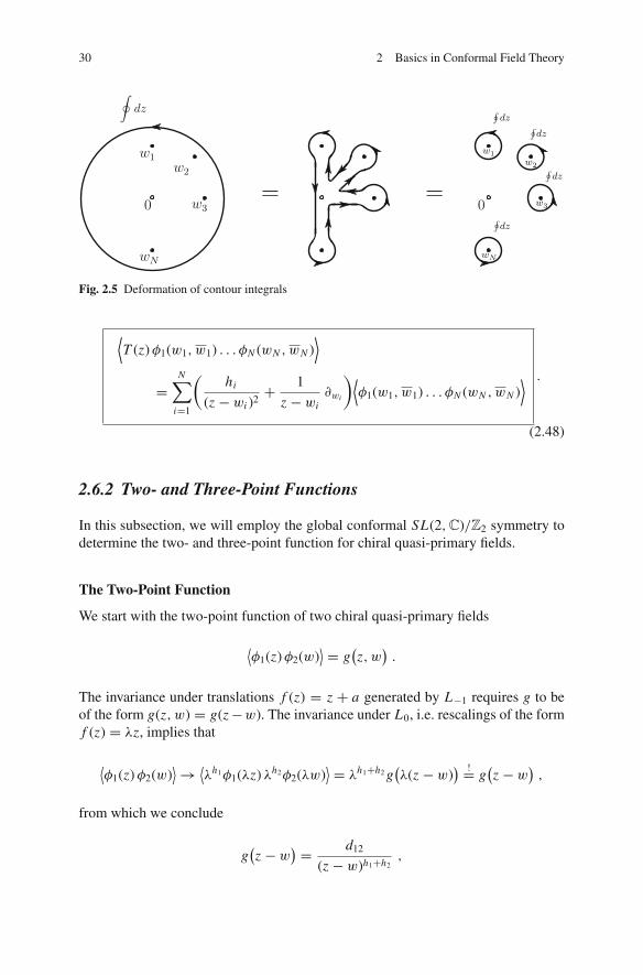
where we have applied the deformation of the contour integrals illustrated in Fig. 2.5and used Eq. (2.37). Employing then the two relations shown in Eq. (2.38), we canwrite

0 =∮

dz

2π iε(z)

[

⟨

T (z) φ1(w1, w1) . . . φN (wN , wN )⟩

(2.47)

−N∑

i=1

(

hi

(z − wi )2+ 1

z − wi�wi

)

⟨

φ1(w1, w1) . . . φN (wN , wN )⟩

]

Since this must hold for all ε(z) of the form ε(z) = −zn+1 with n ∈ Z, the integrandmust already vanish and we arrive at the Conformal Ward identity


= =0

w1w2

w3

wN

∮dz

0

w1w2

w3

wN

dz

dz

dz

dz

∮∮

∮

∮

Fig. 2.5 Deformation of contour integrals

⟨

T (z) φ1(w1, w1) . . . φN (wN , wN )⟩

=N∑

i=1

(

hi

(z − wi )2+ 1

z − wi�wi

)

⟨

φ1(w1, w1) . . . φN (wN , wN )⟩ .

(2.48)

2.6.2 Two- and Three-Point Functions

In this subsection, we will employ the global conformal SL(2, C)/Z2 symmetry todetermine the two- and three-point function for chiral quasi-primary fields.

The Two-Point Function

We start with the two-point function of two chiral quasi-primary fields

⟨

φ1(z) φ2(w)⟩ = g

(

z, w)

.

The invariance under translations f (z) = z + a generated by L−1 requires g to beof the form g(z, w) = g(z −w). The invariance under L0, i.e. rescalings of the formf (z) = λz, implies that

⟨

φ1(z) φ2(w)⟩ → ⟨

λh1φ1(λz) λh2φ2(λw)⟩ = λh1+h2 g

(

λ(z − w)) != g

(

z − w)

,

from which we conclude

g(

z − w) = d12

(z − w)h1+h2,


where d12 is called a structure constant. Finally, the invariance of the two-pointfunction under L1 essentially implies the invariance under transformations f (z) =− 1

z for which we find

⟨

φ1(z) φ2(w)⟩ → ⟨ 1

z2h1

1

w2h2φ1

(−1

z

)

φ2(− 1

w

)⟩

= 1

z2h1w2h2

d12(− 1

z + 1w

)h1+h2

!= d12

(z − w)h1+h2

which can only be satisfied if h1 = h2. We therefore arrive at the result that

The SL(2, C)/Z2 conformal symmetry fixes the two-point function oftwo chiral quasi-primary fields to be of the form

⟨

φi (z) φ j (w)⟩ = di j δhi ,h j

(z − w)2hi. (2.49)

As an example, let us consider the energy–momentum tensor T (z). From theOPE shown in Eq. (2.41) (and using the fact that one-point functions of conformalfields on the sphere vanish), we find that

⟨

T (z) T (w)⟩ = c/2

(z − w)4.

The Three-Point Function

After having determined the two-point function of two chiral quasi-primary fieldsup to a constant, let us now consider the three-point function. From the invarianceunder translations, we can infer that

⟨

φ1(z1) φ2(z2) φ3(z3)⟩ = f (z12, z23, z13) ,

where we introduced zi j = zi − z j . The requirement of invariance under dilationcan be expressed as

⟨

φ1(z1) φ2(z2) φ3(z3)⟩ → ⟨

λh1φ1(λz1) λh2φ2(λz2) λh3φ3(λz3)⟩

= λh1+h2+h3 f ( λz12, λz23, λz13 )!= f ( z12, z23, z13 )

from which it follows that


f (z12, z23, z13) = C123

za12 zb

23 zc13

,

with a + b + c = h1 + h2 + h3 and C123 some structure constant. Finally, from theSpecial Conformal Transformations, we obtain the condition

1

z2h11 z2h2

2 z2h33

(z1z2)a (z2z3)b (z1z3)c

za12 zb

23 zc13

= 1

za12 zb

23 zc13

.

Solving this expression for a, b, c leads to

a = h1 + h2 − h3 , b = h2 + h3 − h1 , c = h1 + h3 − h2 ,

and so we have shown that

The SL(2, C)/Z2 conformal symmetry fixes the three-point function ofchiral quasi-primary fields up to a constant to

⟨

φ1(z1) φ2(z2) φ3(z3)⟩ = C123

zh1+h2−h312 zh2+h3−h1

23 zh1+h3−h213

. (2.50)

Remarks

• Using the SL(2, C)/Z2 global symmetry, it is possible to map any three points{z1, z2, z3} on the Riemann sphere to {0, 1,∞}.

• The results for the two- and three-point function have been derived using onlythe SL(2, C)/Z2 � SO(3, 1) symmetry. As we have mentioned before, the con-formal group SO(3, 1) extends to higher dimensions R

d,0 as SO(d + 1, 1). Byanalogous reasoning, the two- and three-point functions for CFTs in dimensionsd > 2 then have the same form as for d = 2.

• In order for the two-point function (2.49) to be single-valued on the complexplane, that is, to be invariant under rotations z �→ e2π i z, we see that the conformaldimension of a chiral quasi-primary field has to be integer or half-integer.

2.6.3 General Form of the OPE for Chiral Quasi-Primary Fields

General Expression for the OPE

The generic form of the two- and three-point functions allows us to extract the gen-eral form of the OPE between two chiral quasi-primary fields in terms of other


quasi-primary fields and their derivatives1. To this end we make the ansatz

φi (z) φ j (w) =∑

k,n≥0

Cki j

ani jk

n!

1

(z − w)hi +h j −hk−n�nφk(w) , (2.51)

where the (z−w) part is fixed by the scaling behaviour under dilations z �→ λz. Notethat we have chosen our ansatz such that an

i jk only depends on the conformal weightshi , h j , hk of the fields i, j, k (and on n), while Ck

i j contains further information aboutthe fields.

Let us now take w = 1 in Eq. (2.51) and consider it as part of the followingthree-point function:

⟨ (

φi (z) φ j (1))

φk(0)⟩

=∑

l,n≥0

Cli j

ani jl

n!

1

(z − 1)hi +h j −hl−n

⟨

�nφl(1) φk(0)⟩

.

Using then the general formula for the two-point function (2.49), we find for thecorrelator on the right-hand side that

⟨

�nz φl(z)φk(0)

⟩

∣

∣

∣

z=1= �n

z

(

dlk δhl ,hk

z2hk

)∣

∣

∣

∣

z=1

= (−1)n n!

(

2hk + n − 1

n

)

dlk δhl ,hk .

We therefore obtain

⟨

φi (z) φ j (1) φk(0)⟩ =

∑

l,n≥0

Cli j dlk an

i jk

(

2hk + n − 1

n

)

(−1)n

(z − 1)hi +h j −hk−n. (2.52)

However, we can also use the general expression for the three-point function (2.50)with values z1 = z, z2 = 1 and z3 = 0. Combining then Eq. (2.50) with Eq. (2.52),we find

∑

l,n≥0

Cli j dlk an

i jk

(

2hk + n − 1

n

)

(−1)n

(z − 1)hi +h j −hk−n!= Ci jk

(z − 1)hi +h j −hk zhi +hk−h j,

∑

l,n≥0

Cli j dlk an

i jk

(

2hk + n − 1

n

)

(−1)n (z − 1)n != Ci jk(

1 + (z − 1))hi +hk−h j

.

Finally, we use the following relation with x = z − 1 for the term on the right-handside of the last formula:

1 The proof that the OPE of two quasi-primary fields involves indeed just other quasi-primaryfields and their derivatives is non-trivial and will not be presented.


1

(1 + x)H=

∞∑

n=0

(−1)n

(

H + n − 1

n

)

xn .

Comparing coefficients in front of the (z − 1) terms, we can fix the constants Cli j

and ani jk and arrive at the result that

The OPE of two chiral quasi-primary fields has the general form

φi (z) φ j (w) =∑

k,n≥0

Cki j

ani jk

n!

1

(z − w)hi +h j −hk−n�nφk(w) (2.53)

with coefficients

ani jk =

(

2hk + n − 1

n

)−1(hk + hi − h j + n − 1

n

)

,

Ci jk = Cli j dlk .

General Expression for the Commutation Relations

The final expression (2.53) gives a general form for the OPE of chiral quasi-primaryfields. However, as we have seen previously, the same information is encoded inthe commutation relations of the Laurent modes of the fields. We will not derivethese commutators but just summarise the result. To do so, we recall the Laurentexpansion of chiral fields φi (z)

φi (z) =∑

m

φ(i)m z−m−hi ,

where the conformal dimensions hi of a chiral quasi-primary field are always integeror half-integer. Note that here i is a label for the fields and m ∈ Z or m ∈ Z + 1

2denotes a particular Laurent mode. After expressing the modes φ(i)m as contourintegrals over φi (z) and performing a tedious evaluation of the commutator, onearrives at the following compact expression for the algebra:

[

φ(i)m, φ( j)n] =

∑

k

Cki j pi jk(m, n) φ(k)m+n + di j δm,−n

(

m + hi − 1

2hi − 1

)

(2.54)

with the polynomials


pi jk(m, n) =∑

r,s ∈ Z+0

r+s=hi +h j −hk−1

Ci jkr,s ·

(−m + hi − 1

r

)

·(−n + h j − 1

s

)

,

Ci jkr,s = (−1)r

(

2hk − 1)

!(

hi + h j + hk − 2)

!

s−1∏

t=0

(

2hi − 2 − r − t)

r−1∏

u=0

(

2h j − 2 − s − u)

.

(2.55)

Remarks

• Note that on the right-hand side of Eq. (2.54), only fields with conformal dimen-sion hk < hi + h j can appear. This can be seen by studying the coefficients(2.55).

• Furthermore, because the polynomials pi jk depend only on the conformal di-mensions hi , h j , h j of the fields i, j, k, it is also common to use the conformaldimensions as subscripts, that is, phi h j h j .

• The generic structure of the chiral algebra of quasi-primary fields (2.53) is ex-tremely helpful for the construction of extended symmetry algebras. We willconsider such so-called W algebras in Sect. 3.7.

• Clearly, not all fields in a conformal field theory are quasi-primary and so theformulas above do not apply for all fields! For instance, the derivatives �nφk(z)of a quasi-primary field φ(z) are not quasi-primary.

Applications I: Two-Point Function Revisited

Let us now consider four applications of the results obtained in this section. First,with the help of Eq. (2.54), we can compute the norm of a state φ(i)−n|0〉. Assumingn ≥ h, we obtain

∣

∣

∣

∣ φ(i)−n

∣

∣0⟩ ∣

∣

∣

∣

2 = ⟨

0∣

∣ φ†(i)−n φ(i)−n

∣

∣0⟩

= ⟨

0∣

∣ φ(i)+n φ(i)−n

∣

∣0⟩

= ⟨

0∣

∣

[

φ(i)+n, φ(i)−n]∣

∣0⟩

= C jii phi hi h j (n,−n)

⟨

0∣

∣ φ( j)0

∣

∣0⟩ + dii

(

n + hi − 1

2hi − 1

)

= dii

(

n + hi − 1

2hi − 1

)

.

Employing then Eq. (2.28) as well as Eq. (2.32), we see that the norm of a state|φ〉 = φ−h |0〉 is equal to the structure constant of the two-point function

⟨

φ∣

∣φ⟩ = ⟨

0∣

∣φ+h φ−h

∣

∣0⟩ = dφφ . (2.56)


Applications II: Three-Point Function Revisited

Let us also determine the structure constant of the three-point function betweenchiral quasi-primary fields. To do so, we write Eq. (2.50) as

C123 = zh1+h2−h312 zh2+h3−h1

23 zh1+h3−h213

⟨

φ1(z1) φ2(z2) φ3(z3)⟩

,

and perform the limits z1 → ∞, z3 → 0 while keeping z2 finite. Using then again(2.28) as well as (2.32), we find

C123 = limz1→∞ lim

z3→0zh1+h2−h3

12 zh2+h3−h123 zh1+h3−h2

13

⟨

φ1(z1) φ2(z2) φ3(z3)⟩

= limz1→∞ lim

z3→0z2h1

1 zh2+h3−h12

⟨

φ1(z1) φ2(z2) φ3(z3)⟩

=zh2+h3−h12

⟨

0∣

∣ φ(1)+h1 φ2(z2) φ(3)−h3

∣

∣0⟩

.

Because the left-hand side of this equation is a constant, the right-hand side can-not depend on z2 and so only the z0

2 term does give a non-trivial contribution. Wetherefore conclude that

C123 = ⟨

0∣

∣ φ(1)+h1 φ(2)h3−h1 φ(3)−h3

∣

∣0⟩

. (2.57)

Applications III: Virasoro Algebra

After studying the two- and three-point function, let us now turn to the Virasoroalgebra and determine the structure constants Ck

i j and di j . From the general expres-sion (2.54), we infer the commutation relations between the Laurent modes of theenergy–momentum tensor to be of the following form:

[

Lm, Ln] = C L

L L p222(m, n) Lm+n + dL L δm,−n

(

m + 1

3

)

,

where in view of the final result, we identified CkL L = 0 for k �= L . Note also that the

subscripts of pi jk denote the conformal weight of the chiral fields involved. Usingthe explicit expression (2.55) for pi jk and recalling from p. 29 that the conformaldimension of T (z) is h = 2, we find

p222(m, n) = C2221,0

(−m + 1

1

)

+ C2220,1

(−n + 1

1

)

with coefficients C222r,s of the form

C2221,0 = (−1)1 · 3!

4!· 2 = −1

2and C222

0,1 = (−1)0 · 3!

4!· 2 = +1

2.

Putting these results together, we obtain for the Virasoro algebra

2.7 Normal Ordered Products 37

[

Lm, Ln] = C L

L L

m − n

2Lm+n + dL L δm,−n

m3 − m

6.

If we compare with Eq. (2.16), we can fix the two unknown constants as

dL L = c

2, C L

L L = 2 . (2.58)

Applications IV: Current Algebras

Finally, let us study the so-called current algebras. The definition of a current in atwo-dimensional conformal field theory is the following:

Definition 7. A chiral field j(z) with conformal dimension h = 1 is called a current.A similar definition holds for the anti-chiral sector.

Let us assume we have a theory with N quasi-primary currents ji (z) where i =1, . . . , N . We can express these fields as a Laurent series ji (z) = ∑

n∈Zz−n−1 j(i)n in

the usual way and determine the algebra of the Laurent modes j(i)n using Eq. (2.54)

[

j(i)m, j( j)n] =

∑

k

Cki j p111(m, n) j(k)m+n + di j m δm,−n . (2.59)

From Eq. (2.55), we compute p111(m, n) = 1 and so it follows that Cki j = −Ck

ji dueto the anti-symmetry of the commutator.

Next, we perform a rotation among the fields such that the matrix di j is diag-onalised, and by a rescaling of the fields we can achieve di j → k δi j where k issome constant. Changing then the labels of the fields from subscript to superscriptand denoting the constants Ck

i j in the new basis by f i jk , we can express the algebraEq. (2.59) as

[

j im, j j

n

] =∑

l

f i jl j lm+n + k m δi j δm,−n , (2.60)

where f i jl are called structure constants and k is called the level. As it turns out,the algebra (2.60) is a generalisation of a Lie algebra called a Kac–Moody algebrawhich is infinite dimensional. conformal field theories based on such algebras pro-vide many examples of abstract CFTs which we will study in much more detail inChap. 3.

2.7 Normal Ordered Products

Operations on the field space of a theory are provided by the action of derivatives�φi , �2φi , . . . and by taking products of fields at the same point in space–time. Asknown from quantum field theory, since the φi are operators, we need to give an


ordering prescription for such products. This will be normal ordering which inQFT language means “creation operators to the left”.

In this section, we will illustrate that the regular part of an OPE provides a notionof normal ordering for the product fields.

Normal Ordering Prescription

Let us start by investigating what are the creation and what are the annihilationoperators in a CFT. To do so, we recall Eq. (2.27) which reads

φn,m

∣

∣0⟩ = 0 for n > −h, m > −h . (2.61)

From here we can see already that we can interpret operators φn,m with n > −h orm > −h as annihilation operators.

However, in order to explore this point further, let us recall from Eq. (2.24) thatthe Hamiltonian is expressed in terms of L0 and L0 as H = L0 + L0, which moti-vates the notion of “chiral energy” for the L0 eigenvalue of a state. For the specialcase of a chiral primary, let us calculate

L0 φn

∣

∣0⟩ = (

L0 φn − φn L0) ∣

∣0⟩ = [

L0, φn] ∣

∣0⟩ = −n φn

∣

∣0⟩

, (2.62)

where we employed Eq. (2.45) as well as L0 |0〉 = 0. Taking into account (2.61),we see that the chiral energy is bounded from below, i.e. only values (h + m) withm ≥ 0 are allowed. Requiring that creation operators should create states withpositive energy, we conclude that

φn with n > −h are annihilation operators ,

φn with n ≤ −h are creation operators .

The anti-chiral sector can be included by following the same arguments for L0.Coming then back to the subject of this paragraph, the normal ordering prescriptionis to put all creation operators to the left.

Normal Ordered Products and OPEs

After having discussed the normal ordering prescription for operators in a conformalfield theory, let us state that

The regular part of an OPE naturally gives rise to normal ordered prod-ucts (NOPs) which can be written in the following way:

φ(z) χ (w) = sing. +∞∑

n=0

(z − w)n

n!N(

χ�nφ)

(w) . (2.63)

2.7 Normal Ordered Products 39

The notation for normal ordering we will mainly employ is N (χφ), however, it isalso common to use : φχ :, (φχ ) or [φχ ]0. In the following, we will verify thestatement above for the case n = 0.

Let us first use Eq. (2.63) to obtain an expression for the normal ordered productof two operators. To do so, we apply 1

2π i

∮

dz(z − w)−1 to both sides of Eq. (2.63)which picks out the n = 0 term on the right-hand side leading to

N(

χ φ)

(w) =∮

C(w)

dz

2π i

φ(z)χ (w)

z − w. (2.64)

However, we can also perform a Laurent expansion of N (χφ) in the usual waywhich gives us

N(

χ φ)

(w) =∑

n∈Z

w−n−hφ−hχ

N(

χ φ)

n ,

N(

χ φ)

n =∮

C(0)

dw

2π iwn+hφ+hχ −1 N

(

χ φ)

(w) , (2.65)

where we also include the expression for the Laurent modes N (χ φ)n . Let us nowemploy the relation (2.64) in Eq. (2.65) for which we find

N(

χ φ)

n =∮

C(0)

dw

2π iwn+hφ+hχ−1

∮

C(w)

dz

2π i

φ(z)χ (w)

z − w(2.66)

=∮

dw

2π iwn+hφ+hχ−1

(∮

|z|>|w|

dz

2π i

φ(z)χ (w)

z − w︸︷︷︸

I1︸︷︷︸

I2

−∮

|z|<|w|

dz

2π i

χ (w)φ(z)

z − w

)

where we applied the deformation of contour integrals formulated in Eq. (2.36).Expressing φ and χ as a Laurent series, the term I1 can be evaluated as

I1 =∮

|z|>|w|

dz

2π i

1

z − w

∑

r,s

z−r−hφ

w−s−hχ

φr χs

=∮

|z|>|w|

dz

2π i

1

z

∑

p≥0

(

w

z

)p∑

r,s

z−r−hφ

w−s−hχ

φr χs

=∮

|z|>|w|

dz

2π i

∑

p≥0

∑

r,s

z−r−hφ−p−1w−s−hχ +p φr χs .

Note that we employed 1z−w

= 1z(1−w/z) as well as the geometric series to go from

the first to the second line and that only the z−1 term gives a non-zero contribution.Thus, performing the integral over dz leads to a δ-function setting r = −hφ − p and


so the integral I2 reads

I2 =∮

dw

2π i

∑

p≥0

∑

s

w−s−hχ +p+n+hφ+hχ−1 φ−hφ−p χs ,

for which again only the w−1 term contributes and therefore s = p + n + hφ . Wethen arrive at the final expression for the first term in N (χφ)n

I2 =∑

p≥0

φ−hφ−p χhφ+n+p =∑

k≤−hφ

φk χn−k .

For the second term, we perform a similar calculation to find∑

k>−hφ χn−kφk , whichwe combine into the final result for the Laurent modes of normal ordered products

N(

χ φ)

n =∑

k>−hφ

χn−k φk +∑

k≤−hφ

φk χn−k . (2.67)

Here we see that indeed the φk in the first term are annihilation operators at the rightand that the φk in the second term are creation operators at the left. Therefore, theregular part of an OPE contains normal ordered products.

Useful Formulas

For later reference, let us now consider a special case of a normal ordered product.In particular, let us compute N (χ�φ)n and N (�χφ)n for which we note that theLaurent expansion of say �φ can be inferred from φ in the following way:

�φ(z) = �∑

n

z−n−h φn =∑

n

(−n − h) z−n−(h+1) φn . (2.68)

Replacing φ → �φ in Eq. (2.66), using the Laurent expansion (2.68) and performingthe same steps as above, one arrives at the following results:

N(

χ �φ)

n =∑

k>−hφ−1

(−hφ − k)

χn−k φk +∑

k≤−hφ−1

(−hφ − k)

φk χn−k ,

N(

�χ φ)

n =∑

k>−hφ

(−hχ − n + k) χn−k φk +∑

k≤−hφ

(−hχ − n + k) φk χn−k .

(2.69)

Normal Ordered Products of Quasi-Primary Fields

Let us also note that normal ordered products of quasi-primary fields are in generalnot quasi-primary, but can be projected to such. To illustrate this statement, weconsider the example of the energy–momentum tensor. Recalling the OPE (2.41)

2.8 The CFT Hilbert Space 41

together with Eq. (2.63), we can write

T (z)T (w) = c/2

(z − w)4+ 2 T (w)

(z − w)2+ �T (w)

z − w+ N

(

T T)

(w) + . . . . (2.70)

However, using the general expression for the OPE of two quasi-primary fieldsshown in Eq. (2.53), we observe that there is a �2T term at (z −w)0 with coefficient

CTT T

a2222

2!where a2

222 =(

5

2

)−1(3

2

)

= 3

10and CT

T T = 2 .

(2.71)

But, since the index k in Eq. (2.53) runs over all quasi-primary fields of the theory,we expect also other terms at order (z − w)0. If we denote these by N (T T ), we findfrom Eq. (2.70) that

N(

T T) = N

(

T T) + 3

10�2T .

One can easily check that �2T is not a quasi-primary field, and by computing forinstance [Lm, N (T T )n] and comparing with Eq. (2.45), one arrives at the same con-clusion for N (T T ). However, we note that

N(

T T) = N

(

T T) − 3

10�2T (2.72)

actually is a quasi-primary normal ordered product. Moreover, it turns out that thisprocedure can be iterated which allows one to write the entire field space in termsof quasi-primary fields and derivatives thereof.

2.8 The CFT Hilbert Space

In this section, we are going summarise some general properties of the Hilbert spaceof a conformal field theory.

The Verma Module

Let us consider again the chiral energy–momentum tensor. For the Laurent expan-sions of T (z) and �T (z) as well as for the corresponding asymptotic in-states, wefind


T (z) =∑

n∈Z

z−n−2 Ln ←→ L−2

∣

∣0⟩

,

�T (z) =∑

n∈Z

(−n − 2) z−n−3 Ln ←→ L−3

∣

∣0⟩

,

where we employed the relation (2.28). The state corresponding to the normalordered product of two energy–momentum tensors can be determined as follows.From the Laurent expansion

N(

T T) =

∑

n∈Z

z−n−4 N(

T T)

n,

we see that only the mode with n = −4 gives a well-defined contribution in thelimit z → 0. But from the general expression for the normal ordered product (2.67),we obtain

N(

T T)

n =∑

k>−2

Ln−k Lk +∑

k≤−2

Lk Ln−k ,

where the first sum vanishes when applied to |0〉 and the second sum acting on thevacuum only contributes for n − k ≤ −2. Taking into account that n = −4 fromabove, we find

N(

T T)

−4

∣

∣0⟩ = L−2 L−2

∣

∣0⟩

and N(

T T) ←→ L−2 L−2

∣

∣0⟩

.

Finally, we note that using Eq. (2.69), one can similarly show N(

T �T) ↔ L−3L−2|0〉.

These examples motivate the following statement:

For each state |�〉 in the so-called Verma module

{

Lk1 . . . Lkn

∣

∣0⟩

: ki ≤ −2}

,

we can find a field F ∈ {

T, �T, . . . , N (. . .)}

with the property thatlimz→0 F(z) |0〉 = |�〉.

Conformal Family

Let us consider now a general (chiral) primary field φ(z) of conformal dimension h.This field gives rise to the state |φ〉 = |h〉 = φ−h |0〉 which, due to the definition ofa primary field (2.45), satisfies

Ln

∣

∣φ⟩ = [

Ln, φ−h] ∣

∣0⟩ =

(

h (n + 1) − n)

φ−h+n

∣

∣0⟩ = 0 , (2.73)

2.8 The CFT Hilbert Space 43

for n > 0. Without providing detailed computations, we note that the modes ofthe energy–momentum tensor with n < 0 acting on a state |h〉 correspond to thefollowing fields:

Field State Level

φ(z) φ−h |0〉 = |h〉 0

�φ L−1φ−h |0〉 1

�2φ L−1L−1φ−h |0〉 2

N(

T φ)

L−2φ−h |0〉 2

�3φ L−1L−1L−1φ−h |0〉 3

N(

T �φ)

L−2L−1φ−h |0〉 3

N(

�T φ)

L−3φ−h |0〉 3

. . . . . . . . .

(2.74)

The lowest lying state in such a tower of states, that is |h〉, is called a highest weightstate. From Eq. (2.74), we conclude furthermore that

Each primary field φ(z) gives rise to an infinite set of descendant fieldsby taking derivatives �k and taking normal ordered products with T . Theset of fields

[

φ(z)]

:={

φ , �φ , �2φ , . . . , N(

T φ)

, . . .}

is called a conformal family which is also denoted by{

Lk1 . . . Lkn φ(z) :ki ≤ −1

}

.

Remarks

• Referring to the table in Eq. (2.74), note that there are P(n) different states atlevel n where P(n) is the number of partitions of n. The generating function forP(n) will be important later and reads

∞∏

n=1

1

1 − qn=

∞∑

N=0

P(N ) q N .

• For unitary theories, we know that the norm of all states has to be non-negative. Inparticular, recalling Eq. (2.56), for the structure constant of a two-point functionthis implies dφφ ≥ 0, where φ is a primary field. Let us then consider the normof the state L−1|φ〉 for which we compute


∣

∣

∣

∣ L−1

∣

∣φ⟩ ∣

∣

∣

∣

2 = ⟨

φ∣

∣ L+1 L−1

∣

∣φ⟩ = ⟨

φ∣

∣

[

L+1, L−1]∣

∣φ⟩ = ⟨

φ∣

∣ 2L0

∣

∣φ⟩ = 2 h dφφ,

where we employed Eq. (2.73) as well as the Virasoro algebra (2.16). In order forthis state to have non-negative norm, we see that h ≥ 0. Therefore, a necessarycondition for a theory to be unitary is that the conformal weights of all primaryfields are non-negative.

2.9 Simple Examples of CFTs

So far, we have outlined part of the generic structure of conformal field theorieswithout any reference to a Lagrangian formulation. In particular, we introducedCFTs via OPEs, respectively, operator algebras which, as we will see later, is ex-tremely powerful for studying CFTs and in certain cases leads to a complete solutionof the dynamics. However, to make contact with the usual approach to quantum fieldtheories and because they naturally appear in string theory, let us consider threesimple examples of conformal field theories given in terms of a Lagrangian action.

2.9.1 The Free Boson

Motivation

Let us start with a real massless scalar field X (x0, x1) defined on a cylinder givenby x0 ∈ R and x1 ∈ R subject to the identification x1 � x1 + 2π . The action forsuch a theory takes the following form:

S = 1

4πκ

∫

dx0 dx1√

|h| hαβ �α X�β X

= 1

4πκ

∫

dx0 dx1(

(

�x0 X)2 + (

�x1 X)2)

(2.75)

where h = det hαβ with hαβ = diag(+1,+1), and κ is some normalisation constant.This is the (Euclideanised) world-sheet action (in conformal gauge) of a string mov-ing in a flat background with coordinate X . Since in this theory there is no mass termsetting a scale, we expect this action to be conformally invariant.

In order to study the action (2.75) in more detail, as we have seen in Sect. 2.4, itis convenient to map the cylinder to the complex plane which is achieved by

z = ex0 · eix1. (2.76)

Performing this change of variables for the action (2.75) and denoting the new fieldsby X (z, z), we find

2.9 Simple Examples of CFTs 45

S = 1

4πκ

∫

dz dz√

|g| gab �a X�b X (2.77)

= 1

4πκ

∫

dz dz �X · �X (2.78)

with a, b standing for z and z. Note that here and in the following we will use thenotation � = �z and � = �z interchangeably. Furthermore, in going from Eq. (2.77)to Eq. (2.78), we employed the explicit form of the metric gab which we obtainedvia gab = �xα

�xa�xβ

�xb hαβ and which reads

gab =[

0 12zz

12zz 0

]

, gab =[

0 2zz2zz 0

]

.

Basic Properties

In the last paragraph, we have provided a connection between the string theorynaturally defined on a cylinder and the example of the free boson defined on thecomplex plane. From a conformal field theory point of view, however, we do notneed this discussion but can simply start from the action (2.78)

S = 1

4πκ

∫

dz dz �X · �X . (2.79)

The equation of motion for this action is derived by varying S with respect to X .We thus calculate

0 = δX S

= 1

4πκ

∫

dz dz

(

�δX · �X + �X · �δX

)

= 1

4πκ

∫

dz dz

(

�(

δX · �X)

− δX · ��X + �(

�X · δX)

− ��X · δX

)

= − 1

2πκ

∫

dz dz δX(

��X)

which has to be satisfied for all variations δX . Therefore, we obtain the equation ofmotion as

� � X (z, z) = 0 ,

from which we conclude that

j(z) = i �X (z, z) is a chiral field,

j(z) = i �X (z, z) is an anti-chiral field.(2.80)


Next, we are going to determine the conformal properties of the fields in theaction (2.79). In particular, this action is invariant under conformal transformationsif the field X (z, z) has vanishing conformal dimensions, that is, X ′(z, z) = X (w,w).Let us then compute

S −→ 1

4πκ

∫

dz dz �z X ′(z, z) · �z X ′(z, z)

= 1

4πκ

∫

�z

�wdw

�z

�wdw

�w

�z�w X (w,w) · �w

�z�w X (w,w)

= 1

4πκ

∫

dw dw �w X (w,w) · �w X (w,w)

which indeed shows the invariance of the action (2.79) under conformal transforma-tions if X (z, z) has conformal dimensions (h, h) = (0, 0). Moreover, by consideringagain the calculation above, we can conclude that the fields (2.80) are primary withdimensions (h, h) = (1, 0) and (h, h) = (0, 1) respectively. Finally, because we areconsidering a free theory, the engineering dimensions of the fields argued for aboveis the same as the dimension after quantisation.

Two-Point Function and Laurent Mode Algebra

Let us proceed and determine the propagator K (z, z, w,w) = 〈X (z, z)X (w,w)〉 ofthe free boson X (z, z) from the action (2.79). To do so, we note that K (z, z, w,w)in the present case has to satisfy

�z �z K (z, z, w,w) = −2πκ δ(2)(z − w) .

Using the representation of the δ-function 2πδ(2) = �z z−1, one can then check thatthe following expression is a solution to this equation:

K (z, z, w,w) = ⟨

X (z, z) X (w,w)⟩ = −κ log

∣

∣z − w∣

∣

2, (2.81)

which gives the result for the two-point function of X (z, z). In particular, by com-paring with Eq. (2.49), we see again that the free boson itself is not a quasi-primaryfield. However, from the propagator above we can deduce the two-point function ofsay two chiral fields j(z) by applying derivatives �z and �w to Eq. (2.81)

−⟨

�z X (z, z) �w X (w,w)⟩ = −κ�z�w

(

− log(

z − w) − log

(

z − w)

)

⟨

j(z) j(w)⟩ = κ

(z − w)2, (2.82)

and along similar lines we obtain the result in the anti-chiral sector as well as〈 j(z) j(w)〉 = 0. We can then summarise that the normalisation constant of thetwo-point function is d j j = κ .


Let us finally recall our discussion on p. 37 about current algebras and determinethe algebra of the Laurent modes of j(z). Since we only have one such (chiral)current in our theory, the anti-symmetry of Ck

i j = −Ckji implies C j

j j = 0 whichleads us to

[

jm, jn] = κ m δm+n,0 . (2.83)

The Energy–Momentum Tensor

We will now turn to the energy–momentum tensor for the theory of the free boson.Since we have an action for our theory, we can actually derive this quantity. Wedefine the energy–momentum tensor for the action (2.77) in the following way:

Tab = 4πκ γ1√|g|

δ Sδgab

, (2.84)

where we have allowed for a to be determined normalisation constant γ and a, bstand for z and z respectively. Performing the variation of the action (2.77) using

δ√

|g| = −1

2

√

|g| gab δgab ,

we find the following result:

Tzz = γ �X�X , Tzz = Tzz = 0 , Tzz = γ �X�X .

However, for a quantum theory we want the expectation value of the energy–momentum tensor to vanish and so we take the normal ordered expression. Fo-cussing only on the chiral part, this reads

T (z) = γ N(

�X�X)

(z) = γ N(

j j)

(z) .

The constant γ can be fixed via the requirement that j(z) is a primary field ofconformal dimension h = 1 with respect to T (z). To do so, we expand the energy–momentum tensor as T (z) = ∑

n∈Zz−n−2 Ln and find for the Laurent modes

Ln = γ N(

j j)

n = γ∑

k>−1

jn−k jk + γ∑

k≤−1

jk jn−k , (2.85)

where we used the expression for normal ordered products derived in Sect. 2.7.Recalling the Laurent expansion (2.84) of j(z), we can compute the following com-mutator:


[

Lm, jn] = γ

[

N(

j j)

m, jn]

= γ∑

k>−1

(

jm−k[

jk, jn] + [

jm−k, jn]

jk)

+ γ∑

k≤−1

(

jk[

jm−k, jn] + [

jk, jn]

jm−k

)

= γ κ(∑

k>−1

jm−k k δk,−n + (m − k) δm−k,−n jk

+∑

k≤−1

jk (m − k) δm−k,−n + k δk,−n jm−k

)

= − 2γ κn jm+n ,

where we employed Eq. (2.83). If we compare this expression with Eq. (2.45), wesee that for 2γ κ = 1 this is the commutator of Lm with a primary field of conformaldimension h = 1. Therefore, we can conclude that the energy–momentum tensorreads

T (z) = 1

2κN(

j j)

(z) . (2.86)

The Central Charge

After having determined the energy–momentum tensor T (z) up to a constant, wecan now ask what is the central charge of the free boson conformal field theory. Todetermine c we employ the Virasoro algebra to compute

⟨

0∣

∣L+2L−2

∣

∣0⟩ = ⟨

0∣

∣

[

L2, L−2]∣

∣0⟩ = c

2, (2.87)

where we used that Ln|0〉 = 0 for n > −2. Next, we recall L∓2 = 12κ

N ( j j)∓2 fromwhich we find

L−2

∣

∣0⟩ = 1

2κj−1 j−1

∣

∣0⟩

,⟨

0∣

∣L+2 = 1

2κ

⟨

0∣

∣

(

j2 j0 + j1 j1)

= 1

2κ

⟨

0∣

∣ j1 j1 ,

where we used that⟨

0∣

∣ j2 j0 = −⟨

0∣

∣ j0 j2 = 0. Employing these expressions inEq. (2.87), we obtain


c

2= 1

4κ2

⟨

0∣

∣ j1 j1 j−1 j−1

∣

∣0⟩

= 1

4κ2

(

⟨

0∣

∣ j1 j−1 j1 j−1

∣

∣0⟩ + ⟨

0∣

∣ j1[

j1, j−1]

︸︷︷︸

κ

j−1

∣

∣0⟩

)

= 1

4κ2

(

⟨

0∣

∣

[

j1, j−1][

j1, j−1]∣

∣0⟩ + κ

⟨

0∣

∣

[

j1, j−1]∣

∣0⟩

)

= 1

4κ22κ2 = 1

2

where we employed [ j1, j−1] = κ as well as that jk |0〉 = 0 for k > −1 and that〈0| jk = 0 for k < 1. We have therefore shown

The conformal field theory of a free boson has central charge c = 1.

Remarks

• Let us make contact with our discussion in Sect. 2.6.3 and compare our resultsto Eq. (2.58). First, by recalling equation (2.56) we obtain from Eq. (2.87) thatdL L = c

2 . Second, with the help of Eq. (2.57) we can determine CL L L as follows:

CL L L = ⟨

0∣

∣L2 L0 L−2

∣

∣0⟩ = ⟨

0∣

∣L2[

L0, L−2]∣

∣0⟩ = 2

⟨

0∣

∣L2 L−2

∣

∣0⟩ = 2

c

2= c

where we also employed Eq. (2.87). Finally, referring to p. 34, we use Cki j =

Ci jl (dlk)−1 to find C LL L = 2 which is in agreement with Eq. (2.58). Therefore, as

expected, the Laurent modes of the energy–momentum tensor (2.86) of the freeboson satisfy the Virasoro algebra.

• Note that on p. 16, we have chosen the normalisation of the central extensionp(2,−2) in such a way that we obtain c = 1 for the free boson.

• Usually, one chooses the normalisation constant κ to be κ = 1 in order tosimplify various expressions such as

⟨

j(z) j(w)⟩ = 1

(z − w)2and T (z) = 1

2N(

j j)

(z) . (2.88)

Centre of Mass Position and Momentum

Let us come back to the chiral and anti-chiral currents from Eq. (2.80) and recallonce more their Laurent expansion

j(z) = i �X (z) =∑

n∈ Z

jnz−n−1 , j(z) = i �X (z) =∑

n∈ Z

j nz−n−1 ,

which we can integrate to find


X (z, z) = x0 − i(

j0 ln z + j0 ln z)

+ i∑

n �=0

1

n

(

jn z−n + j n z−n)

. (2.89)

If we identify z with the complex conjugate z∗ of z, then the field X is defined onthe complex plane. As such, it has to be invariant under rotations z �→ e2π i z which,referring to Eq. (2.89), implies that

j0 = j0 . (2.90)

However, as we will see in Sect. 4.2.2, for the free boson X (z, z) compactified on acircle, this relation will be modified.

Let us furthermore recall from the beginning of this section that the example ofthe free boson can be related to string theory. In particular, using the mapping (2.76),we can express Eq. (2.89) in terms of coordinates x0 and x1 on the cylinder

X(

x0, x1) = x0 − i

(

j0 + j0

)

x0 + (

j0 − j0

)

x1

+ i∑

n �=0

1

n

(

jn e−n(x0+i x1) + j n e−n(x0−i x1))

.

Computing the centre of mass momentum π0 of a string, we obtain

π0 = 1

4π

∫ 2π

0dx1 �X

(

x0, x1)

�(−i x0

) = j0 + j0

2= j0 , (2.91)

where the additional factor of (−i) is due to the fact that we are working withEuclidean signature. Similarly, the following expression

1

2π

∫ 2π

0dx1 X

(

x0 = 0, x1) = x0

shows that x0 is the centre of mass coordinate of a string. Performing then the usualquantisation, not only jn and j n are promoted to operators but also x0. Since x0 andπ0 are the position, and momentum operator, respectively, we naturally impose thecommutation relation

[

x0 , π0] = i . (2.92)

Vertex Operator

As we have mentioned earlier, the free boson X (z, z) is not a conformal field sinceits conformal dimensions vanish (h, h) = (0, 0). However, using X (z, z) we candefine the so-called vertex operators which have non-vanishing conformal weights.


The vertex operator V (z, z) =: eiαX (z,z) : is a primary field of confor-mal dimension (h, h) = ( α2

2 , α2

2 ) with respect to the energy–momentumtensors T (z) = 1

2 N ( j j)(z) and T (z) = 12 N ( j j)(z).

Here we have used the notation : . . . : to denote the normal ordering which is alsocommon in the literature. In the following, we will verify that this vertex operatorhas indeed the conformal dimensions stated above.

To do so, we start by making the expression for the vertex operator more concreteusing Eq. (2.89). Keeping in mind that jn for n > −1 are annihilation operators, wecan perform the normal ordering to obtain

V (z, z) = exp

(

iαx0 − α∑

n≤−1

jnn

z−n

)

· exp

(

απ0 ln z − α∑

n≥1

jnn

z−n

)

· v(z) ,

(2.93)

where for convenience we have put all the anti-holomorphic dependence into v(z).Next, let us compute the j0 eigenvalue of this vertex operator which we can inferfrom [ j0, V ]. Because of [ jm, jn] = m δm,−n , we see that j0 commutes with all jnand so we only need to evaluate

[

j0, eiαx0] =

∞∑

k=0

(iα)k

k!

[

j0, xk0

]

︸︷︷︸

= k (−i) xk−10

= −∞∑

k=1

i (iα)k

(k − 1)!xk−1

0 = −i (iα) eiαx0 ,

(2.94)

where we employed Eq. (2.92). We therefore find that [ j0, V ] = αV . Recalling thenour definition Eq. (2.28) of an asymptotic state and computing

j0∣

∣α⟩ = lim

z,z→0

[

j0, Vα(z, z)] ∣

∣0⟩ = lim

z,z→0α V (z, z)

∣

∣0⟩ = α

∣

∣α⟩

,

we see that the j0 eigenvalue of the vertex operator (2.93) is α.Now, we are going to determine the conformal dimension of the vertex opera-

tor (2.93) by computing the commutator [L0, V ]. To do so, let us first recall fromEq. (2.88) the explicit form of L0

L0 = 1

2j0 j0 + 1

2

∑

k≥1

j−k jk + 1

2

∑

k≤−1

jk j−k .

Next, we note again that only j0 has non-trivial commutation relations with x0 sowe find for the first factor in Eq. (2.93)

[

L0, eiαx0] = 1

2

[

j0 j0, eiαx0] = α

2

(

j0 eiαx0 + eiαx0 j0)

. (2.95)


For the terms in Eq. (2.93) involving the modes jn with n �= 0, let us define

J− = −∑

n≤−1

jnn

z−n , J+ = −∑

n≥1

jnn

z−n ,

for which we calculate using [L0, jn] = −n jn

[

L0, J−] =∑

n≤−1

jn z−n = z �z J− ,[

L0, J+] = z �z J+ .

Performing then the series expansion of the exponential and employing our findingsfrom above, we can evaluate

[

L0, eα J−] =∞∑

k=0

αk

k!

[

L0,(

J−)k]

=∞∑

k=0

αk

k!k z

(

�J−) (J−)k−1

=∞∑

k=0

αk

k!z �

(

(

J−)k)

= z �(

eα J−),

and we find a similar result for J+. Observing finally that [L0, v(z)] = 0, we arenow in the position to calculate the full commutator of L0 and V (z, z) to determinethe conformal dimension of V (z, z)

[

L0, V (z, z)] = [

L0, eiαx0]

eα J−zαπ0 eα J+

v + eiαx0[

L0, eα J−]zαπ0 eα J+

v

+ eiαx0 eα J−[L0, zαπ0

]

eα J+v + eiαx0 eα J−

zαπ0[

L0, eα J+]v

= α

2

(

j0eiαx0 + eiαx0 j0)


v + eiαx0(

z�zeα J−)

zαπ0 eα J+v

+ 0 + eiαx0 eα J−zαπ0

(

z�zeα J+)

v

= α

2

(



v + z�V (z, z)

− eiαx0 eα J−(z�z zαπ0

)

eα J+v

= α

2

(



v + z�V (z, z)

− α eiαx0 j0 eα J−zαπ0 eα J+

v

= α

2

[

j0, eiαx0]


v + z�V (z, z)

= α2

2V (z, z) + z �V (z, z)

where we used Eqs. (2.94) and (2.95). Let us then again recall our definition (2.28)of an asymptotic state in terms of an operator and compute


L0

∣

∣α⟩ = lim

z,z→0

[

L0, Vα(z, z)] ∣

∣0⟩ = lim

z,z→0

(

α2

2V (z, z) + z �V (z, z)

)

∣

∣0⟩

= α2

2lim

z,z→0V (z, z)

∣

∣0⟩ = α2

2

∣

∣α⟩

.

The conformal weight of a vertex operator Vα(z, z) therefore is h = α2

2 , and a sim-ilar result is obtained in the anti-chiral sector. This verifies our statement from thebeginning of this paragraph regarding the conformal weights of the vertex operator.In order to show that V (z, z) is a primary field, one can compute along similar linesthe commutator [Lm, V (z, z)] |0〉 and compare with the definition of a primary fieldgiven in Eq. (2.45).

Next, let us note that the action of a free boson (2.79) is invariant under trans-formations X (z, z) �→ X (z, z) + a where a is an arbitrary constant. In order for thecorrelator of two vertex operators 〈 Vα Vβ 〉 to respect this symmetry, we infer fromthe definition Vα = : eiαX : the condition α + β = 0. Recalling then our discussionin Sect. 2.6.2 and keeping in mind that Vα(z, z) is a primary field, for the two-pointfunction of two vertex operators we find

⟨

V−α(z, z) Vα(w,w)⟩ = 1

(z − w)α2 (z − w)α2 .

Here we have included the result for the anti-holomorphic sector, which can beobtained in a similar fashion as the holomorphic part. However, we will study non-holomorphic OPEs in much more detail in Sect. 2.12. Since α + β = 0, for thetwo-point function of vertex operators with equal j0 eigenvalues, we have

⟨

V+α V+α

⟩ = ⟨

V−α V−α

⟩ = 0 .

Let us also mention that the current j(z) = i�X (z, z) is conserved and that theconserved charge is Q = ∮

dz2π i j(z) = j0. We can thus interpret α as the charge of

an vertex operator Vα(z, z) and the requirement α + β = 0 as charge conservation.In passing, we note that vertex operators play a very important role in string

theory, where the charge α is interpreted as the space–time momentum along thespace–time direction X . The condition of charge conservation then corresponds tomomentum conservation in space–time.

Current Algebra

After having verified the conformal dimension of the vertex operator Vα =: eiαX :to be (h, h) = ( α2

2 , α2

2 ), let us now turn to the special case α = ±√2 for which

V±√2(z, z) has conformal dimension (h, h) = (1, 1). Therefore, following our def-

inition from p. 37, these fields are currents. In order to simplify our discussion inthis paragraph, let us focus only on the holomorphic part of the vertex operator(including the position operator x0) which we write as


j±(z) = : e±i√

2X : ,

and study the current algebra of j±(z) and j(z) = i(�X )(z). On p. 37, we havegiven the general form of a current algebra of quasi-primary fields which we recallfor convenience

[

j(i)m, j( j)n] =

∑

k

Cki j j(k)m+n + di j m δm,−n , Ck

i j = −Ckji .

Let us then determine the normalisation constants of the two-point function di j . Bythe argument that the overall j0 charge in a correlation function should vanish, wesee that

d j j = d+− = d−+ = 1 , d j± = d± j = 0 ,

where we use subscripts ± for j±(z) and employed the usual normalisation. Next,using Eq. (2.57) as well as relations (2.26) and (2.28), we can compute

C+ j− = ⟨

0∣

∣ j+1 j0 j−

−1

∣

∣0⟩ = lim

z→0

⟨

0∣

∣ j+1 j0 V−√

2(z)∣

∣0⟩

= −√

2⟨

0∣

∣ j+1 j−

−1

∣

∣0⟩

= −√

2 d+− = −√

2 ,

and a similar computation leads to C− j+ = +√2. Noting that also for the three-

point function the overall j0 charge has to vanish and using the relation Ci jk =Cl

i j dlk together with the anti-symmetry of Cki j , we can determine the non-vanishing

structure constants to be

C+j+ = −C+

+ j = +√

2 , C−j− = −C−

− j = −√

2 , C j+− = −C j

−+ .

The only unknown constant C j+− can be fixed using the relation Ci jk = Cl

i j dlk fromp. 34 in the following way:

C j+− = C+− j d j j = C−

− j d−+ d j j =√

2 · 1 · 1

1=

√2 .

Combining all these results, we can finally write down the current algebra of j±(z)and j(z) which reads

[

jm, jn] = m δm+n,0 ,

[

j±m , j±

n

] = 0 ,

[

jm, j±n

] = ±√2 j±

m+n ,[

j+m , j−

n

] = √2 jm+n + m δm+n,0 .

(2.96)


However, in order to highlight the underlying structure, let us make the followingdefinitions:

j1 = 1√2

(

j+ + j−) , j2 = 1√2i

(

j+ − j−) , j3 = j .

The commutation relations for the Laurent modes of the new currents are deter-mined using the relations in Eq. (2.96). We calculate for instance

[

j1m, j2

n

] = 1

2i

(

−[

j+m , j−

n

] + [

j−m , j+

n

]

)

= 1

2i

(−2√

2 jm+n) = +i

√2 j3

m+n ,

[

j3m, j1

n

] = 1√2

[

j3m, j+

n + j−n

] = 1√2

(√2 j+

m+n −√

2 j−m+n

) = +i√

2 j2m+n ,

[

j1m, j1

n

] = 1

2

(

[

j+m , j−

n

] + [

j−m , j+

n

]

)

= 1

2(m − n) δm+n,0 = m δm+n,0 ,

from which we infer the general expression

[

j im, j j

n

] = +i√

2∑

k

εi jk j km+n + m δi j δm,−n

where εi jk is the totally anti-symmetric tensor. These commutation relations define

the su(2) Kac–Moody algebra at level k = 1, which is usually denoted as su(2)1.These algebras are discussed in Chap. 3 in more generality. Furthermore, this currentalgebra is related to the theory of the free boson X compactified on a radius R = 1√

2which we will study in Sect. 4.2.2.

Hilbert Space

Let us note that the Hilbert space of the free boson theory contains for instance thefollowing chiral states:

level 1 : j−1

∣

∣0⟩

,

level 2 : j−2

∣

∣0⟩

, j−1 j−1

∣

∣0⟩

,

level 3 : j−3

∣

∣0⟩

, j−2 j−1

∣

∣0⟩

, j−1 j−1 j−1

∣

∣0⟩

,

. . . . . .

(2.97)

where we have used that [ j−m, j−n] = 0 for m, n ≥ 0. Taking also the anti-chiralsector as well as [ jm, j n] = 0 into account, we can conclude that the Hilbert spaceof the free boson theory is

H = {

Fock space freely generated by j−n, j−m for n, m ≥ 1}

.


The number of states at each level N is given by the number of partitions P(N ) ofN whose generating function we have already encountered at the end of Sect. 2.8.The generating function for the degeneration of states at each level N in the chiralsector therefore is

Z(q) =∏

n≥1

1

1 − qn=

∞∑

N=0

P(N ) q N . (2.98)

Combining now the chiral and anti-chiral sectors, we obtain

Z(q, q) =∏

n≥1

1

(1 − qn)(1 − qn).

In Chap. 4, we will identify such expressions with partition functions of conformalfield theories and relate them to modular forms.

2.9.2 The Free Fermion

Motivation

As a second example for a conformal field theory, we will study the action of afree Majorana fermion in two-dimensional Minkowski space with metric hαβ =diag(+1,−1)

S = 1

4πκ

∫

dx0 dx1√

|h| (−i) � γ α �α � , (2.99)

where κ is a normalisation constant. Here, � is defined as � = �†γ 0 where †denotes hermitian conjugation and the {γ α} are two-by-two matrices satisfying theClifford algebra

γ α γ β + γ β γ α = 2 hαβ 12 ,

with 12 the two-by-two unit matrix. There are various representations of γ -matricessatisfying this algebra which are, however, equivalent. We make the followingchoice:

γ 0 =(

0 11 0

)

, γ 1 =(

0 1−1 0

)

,

for which the Majorana condition becomes that the components ψ,ψ of the spinor� are real. We then perform a Wick rotation x1 → i x1 under which the partialderivative transforms as �1 → −i�1. Effectively, the Wick rotation means choosingthe γ -matrices


γ 0 =(

0 11 0

)

, γ 1 =(

0 −ii 0

)

,

and we furthermore note that the Wick rotation introduces an additional factor of ifor Eq. (2.99). We can simplify the action (2.99) by observing

γ 0 γ μ �μ = γ 0(

γ 0�0 + γ 1�1) =

(

�0 + i�1 00 �0 − i�1

)

= 2

(

�z 00 �z

)

,

where we have defined z = x0 + i x1. As we have seen before, it is convenientto work with fields depending on complex variables and so we write the Majoranaspinors as

� =(

ψ(z, z)

ψ(z, z)

)

.

Note that ψ(z, z) and ψ(z, z) are still real fields, in particular ψ† = ψ and ψ† = ψ .

Employing then the various arguments above, we can write the action (2.99) after aWick rotation in the following way:

S = 1

4πκ

∫

dz dz√

|g| 2 �†(

�z 00 �z

)

�

= 1

4πκ

∫

dz dz(

ψ � ψ + ψ � ψ)

(2.100)

where we used that the components of the metric g, obtained from hαβ via thechange of coordinates z = x0 + i x1, read

gab =[

0 12

12 0

]

, gab =[

0 22 0

]

. (2.101)

Basic Properties

From a conformal field theory point of view, we do not necessarily need the deriva-tion above but can simply start from the action (2.100)

S = 1

4πκ

∫

dz dz(

ψ � ψ + ψ � ψ)

. (2.102)

The equations of motion for this theory are obtained by varying the action withrespect to the fields ψ and ψ which reads


0 = δψ S = 1

4πκ

∫

d2z(

δψ �ψ + ψ�(

δψ)

)

= 1

4πκ

∫

d2z(

δψ �ψ + �(

ψδψ) − (

�ψ)

δψ)

= 1

2πκ

∫

d2z δψ �ψ

where we performed a partial integration on the second term and noted that fermionicfields anti-commute. Since the equation above has to be satisfied for all variationsδψ , we find for the equations of motion

�ψ = �ψ = 0 , (2.103)

where we also included the result for the variation with respect to δψ obtained alongsimilar lines. We can then conclude that ψ = ψ(z) is a chiral field and ψ = ψ(z) isan anti-chiral field.

Next, we will determine the conformal properties of the fields ψ(z) and ψ(z). Byperforming similar steps as for the example of the free boson, we see that the action(2.102) is invariant under conformal transformations if the fields ψ and ψ are pri-mary with conformal dimensions (h, h) = ( 1

2 , 0), and (h, h) = (0, 12 ) respectively.

Let us verify this observation by computing

S −→ 1

4πκ

∫

dz dz(

ψ ′(z, z) �z ψ ′(z, z) + ψ′(z, z) �z ψ

′(z, z)

)

= 1

4πκ

∫

�z

�wdw

�z

�wdw

(

(

�w

�z

) 12

ψ(w,w)�w

�z�w

(

�w

�z

) 12

ψ(w,w)

+(

�w

�z

) 12

ψ(w,w)�w

�z�w

(

�w

�z

) 12

ψ(w,w)

)

= 1

4πκ

∫

dw dw(

ψ(w,w) �w ψ(w,w) + ψ(w,w) �w ψ(w,w))

which shows that the action is indeed invariant under conformal transformations ifψ and ψ are primary fields of conformal dimension 1

2 . Furthermore, because we arestudying a free theory, the engineering dimension 1

2 agrees with the dimension inthe quantum theory.

Finally, let us note that due to the fermionic nature of fields in our theory, thereare two different possibilities for their behaviour under rotations by 2π . In particular,focussing on the chiral sector, on the complex plane we have

ψ(e2π i z) = +ψ(z) Neveu–Schwarz sector (NS),

ψ(e2π i z) = −ψ(z) Ramond sector (R).(2.104)


Radial Ordering and Laurent Expansion

Let us recall that our theory of the free fermion is defined on the complex planewith coordinate z = x0 + i x1, where x0 and x1 are coordinates of R

2. However, wehave seen in Sect. 2.4 and explicitly for the example of the free boson, the quantumtheory is usually defined on a cylinder of infinite length. Without providing a de-tailed derivation, let us just assume we started on a cylinder and have performed themapping to the complex plane giving us our present theory.

This allows us in particular to introduce the concept of radial ordering also forthe fermions. Taking into account the fermionic nature of the fields, we define

R(

�(z)�(w))

:={+�(z) �(w) for |z| > |w| ,

−�(w) �(z) for |w| > |z| .(2.105)

Next, keeping in mind the conformal weight 12 of our fields, we can perform a Lau-

rent expansion of ψ(z) in the usual way

ψ(z) =∑

r

ψr z−r− 12 , (2.106)

and similarly for the anti-chiral field. However, due to the two possibilities shownin Eq. (2.104), the values for r differ between the Neveu–Schwarz and Ramondsectors. It is easy to see that the following choice is consistent with Eq. (2.104):

r ∈ Z + 12 Neveu–Schwarz sector (NS),

r ∈ Z Ramond sector (R).

OPE and Laurent Mode Algebra

Recalling our discussion on p. 34 together with the observation that ψ(z) is a pri-mary field of conformal dimension 1

2 , we can determine the following OPE:

ψ(z) ψ(w) = κ

z − w+ · · · , (2.107)

where the ellipsis denote non-singular terms. The normalisation constant of thetwo-point function κ is the same as in the action (2.102) which can be verified bycomputing the propagator of Eq. (2.102). Note furthermore that this OPE respectsthe fermionic property of ψ since interchanging z ↔ w leads to a minus sign on theright-hand side which is obtained on the left-hand side by interchanging fermions.This fact also explains why there is no single fermion ψ(z) on the right-hand sidebecause (z − w)−

12 ψ(z) would not respect the fermionic nature of the OPE.

Let us now determine the algebra of the Laurent modes of ψ(z). To do so, werecall that the modes in Eq. (2.106) can be expressed in the following way:


ψr =∮

dz

2π iψ(z) zr− 1

2 .

Because the fields under consideration are fermions, we are going to evaluateanti-commutators between the modes ψr and not commutators. Knowing the OPE(2.107), keeping in mind the radial ordering (2.105) and the deformation of contourintegrals illustrated in Fig. 2.4, we calculate

{

ψr , ψs} =

∮

dz

2π i

∮

dw

2π i

{

ψ(z), ψ(w)}

zr− 12 ws− 1

2

=∮

dw

2π iws− 1

2

(∮

|z|>|w|

dz

2π iψ(z)ψ(w) zr− 1

2

−∮

|z|<|w|

dz

2π i− ψ(w)ψ(z) zr− 1

2

)

=∮

dw

2π iws− 1

2

∮

C(w)

dz

2π iR(

ψ(z)ψ(w))

︸︷︷︸

κz−w

zr− 12

= κ

∮

dw

2π iwr+s−1

= κ δr+s,0 . (2.108)

Energy–Momentum Tensor

Let us also determine the energy–momentum tensor from the action (2.102). Forfermionic theories, the definition of Tab differs from the bosonic expression (2.84)and we would have to introduce additional structure to state the explicit form. Letus therefore provide a different but equivalent way to obtain the energy–momentumtensor. The canonical energy–momentum tensor for a theory with fields φi andLagrangian L is defined as

T cμν = 8πκ γ

(

−ημν L +∑

i

�L�(

�μφi)�νφi

)

,

where we allowed for a to be determined normalisation constant γ . However, ingeneral T c is not symmetric but can be made so using the equations of motion.

For the action (2.102), we can compute the canonical energy–momentum tensorusing the metric (2.101) together with the observation that �z = 2 �z as well as�z = 2 �z . We then find

Tzz = γ ψ �ψ , Tzz = −γ ψ �ψ , Tzz = −γ ψ �ψ , Tzz = γ ψ �ψ .

We see that so far, the energy–momentum tensor is not symmetric, but usingEq. (2.103) shows that Tzz = Tzz = 0. In this way, we have arrived at the result


which we would have obtained using a modified form of Eq. (2.84). Focussing thenonly on the chiral part T (z) = Tzz and using at the quantum level the normal orderedexpression, we find

T (z) = γ N(

ψ �ψ)

. (2.109)

To compute the Laurent modes Lm = γ N (ψ�ψ)m of T (z), we note that the deriva-tion in Sect. 2.7 leading to expressions for normal ordered products was done forbosonic fields. For fermionic fields, we need to take into account the modified ra-dial ordering prescription (2.105). Performing then the same analysis, we find forEq. (2.67) in the case of fermionic fields

N(

ψ θ)

r = −∑

s>−hθ

ψr−s θs +∑

s≤−hφ

θs ψr−s . (2.110)

However, employing the same reasoning also for our expression involving deriva-tives (2.69), we can express the Laurent modes of the energy–momentum tensor(2.109) in the following way:

Lm = γ∑

s>− 32

ψm−s ψs

(

s + 1

2

)

− γ∑

s≤− 32

ψs ψm−s

(

s + 1

2

)

. (2.111)

Let us now fix the constant γ by requiring ψ(z) to be a primary field of conformaldimension 1

2 with respect to the energy–momentum tensor (2.109). We thereforecalculate the commutator between the modes Lm and the Laurent modes of the fieldψ(z)

[

Lm, ψr] = + γ

∑

s>− 32

[

ψm−sψs, ψr]

(

s + 1

2

)

− γ∑

s≤− 32

[

ψsψm−s, ψr]

(

s + 1

2

)

= + γ∑

s>− 32

(

s + 1

2

)(

ψm−s{

ψs, ψr} − {

ψm−s, ψr}

ψs

)

− γ∑

s≤− 32

(

s + 1

2

)(

ψs{

ψm−s, ψr} − {

ψs, ψr}

ψm−s

)

= + γ κ∑

s>− 32

(

s + 1

2

)(

ψm−s δs,−r − ψs δm−s,−r

)

− γ κ∑

s≤− 32

(

s + 1

2

)(

ψs δm−s,−r − ψm−s δs,−r

)


= + γ κ

((

−r + 1

2

)

ψm+r −(

m + r + 1

2

)

ψm+r

)

= + γ κ(−m − 2r

)

ψm+r .

If we then choose γ κ = 12 , we find

[

Lm, ψr] =

(

−m

2− r

)

ψm+r ,

and by comparing with Eq. (2.45), we indeed see that ψ(z) is a primary field ofconformal dimension h = 1

2 with respect to the energy–momentum tensor (2.109).In order to simplify the following formulas, let us in the following choose the usualnormalisation:

κ = +1 .

The Central Charge

We will now compute the central charge c of the free fermion theory and start byrecalling a general expression derived previously from the Virasoro algebra

⟨

0∣

∣ L2 L−2

∣

∣0⟩ = c

2.

From Eq. (2.111), we then infer that

L−2 |0〉 = 1

2ψ− 3

2ψ− 1

2

∣

∣0⟩

,⟨

0∣

∣ L2 = 1

2

⟨

0∣

∣

(

ψ 32ψ 1

2+ 2 ψ 1

2ψ 3

2

)

= 1

2

⟨

0∣

∣

(

{

ψ 32, ψ 1

2

} + ψ 12ψ 3

2

)

= 1

2

⟨

0∣

∣ ψ 12ψ 3

2,

and so we calculate using the anti-commutation relations (2.108)

c

2= ⟨

0∣

∣ L2 L−2

∣

∣0⟩ = 1

4

⟨

0∣

∣ ψ 12

ψ 32

ψ− 32

ψ− 12

∣

∣0⟩

= 1

4

⟨

0∣

∣ ψ 12

{

ψ 32, ψ− 3

2

}

ψ− 12

∣

∣0⟩ − 0

= 1

4

⟨

0∣

∣

{

ψ 12, ψ− 1

2

}∣

∣0⟩ − 0 = 1

4.

We therefore conclude that

The central charge of the conformal field theory given by a real freefermion is c = 1

2 .


Complex Fermions and Bosonisation

Let us now turn to a system with two real chiral fermions ψ (1)(z) and ψ (2)(z) whichwe combine into a complex chiral fermion in the following way:

�(z) = 1√2

(

ψ (1)(z) + iψ (2)(z))

. (2.112)

Note that we will always work with chiral quantities so we can denote the complexconjugate of �(z) by �(z) which has, however, no relation with the anti-chiral partor the notation in Eq. (2.99). Furthermore, similarly to the real case, we can expand�(z) in a Laurent series as �(z) = ∑

r �r z−r− 12 and we can easily check that the

modes satisfy

{

�r , �s} = {

�r , �s} = 0 ,

{

�r , �s} = δr+s,0 ,

where we applied the same expansion also for �(z). However, besides these twochiral fields of conformal dimension h = 1

2 , we find now an additional field in thetheory which is expressed as

j(z) = N(

� �)

(z) = −i N(

ψ (1)ψ (2))

(z) . (2.113)

In order to write j(z) in terms of the real fermions ψ (1,2)(z), we have used thatN (ψ (a)ψ (b)) = −N (ψ (b)ψ (a)) with a, b = 1, 2. To verify this relation at the levelof Laurent modes, we write out the normal ordered product (2.110) and perform thechange s → −s + r in the summation index

N(

ψ (a)ψ (b))

r = −∑

s>− 12

ψ(a)r−sψ

(b)s +

∑

s≤− 12

ψ (b)s ψ

(a)r−s

= −∑

s<r+ 12

ψ (a)s ψ

(b)r−s +

∑

s≥r+ 12

ψ(b)r−sψ

(a)s

= −∑

s≤− 12

ψ (a)s ψ

(b)r−s +

∑

s>− 12

ψ(b)r−sψ

(a)s −

r− 12

∑

s= 12

{

ψ (a)s , ψ

(b)r−s

}

= −N(

ψ (b)ψ (a))

r .

Note that the sum over {ψ (a), ψ (b)} = δab δr,0 in the last line gives no contributionsince the summand is only non-zero for r = 0 for which the sum disappears. Fur-thermore, because the modes in general do not (anti-)commute, one has to be carefulwhen changing the summation index.


Let us proceed and perform a series expansion of Eq. (2.113) as j(z) =∑

n jnz−n−1 and investigate the algebra of the modes jn . Writing out the normalordered product and noting that ψ (1)

r and ψ (2)s anti-commute, we find

jm = −i∑

r∈Z+ 12

ψ(1)m−rψ

(2)r .

Here and in the rest of this paragraph, we concentrate on fermions in the Neveu–Schwarz sector with half-integer modes but the result in the Ramond sector is ob-tained in a similar fashion. Employing then that the energy–momentum tensor of�(z) is a sum of the individual ones, we calculate

[

Lm, jn] =

∑

s∈Z+ 12

[

L (1)m + L (2)

m ,−i ψ(1)n−s ψ (2)

s

]

=∑

s∈Z+ 12

(

−i[

L (1)m , ψ

(1)n−s

]

ψ (2)s − i ψ

(1)n−s

[

L (2)m , ψ (2)

s

]

)

=∑

s∈Z+ 12

(

−(

−m

2− n + s

)

i ψ(1)m+n−s ψ (2)

s − i ψ(1)n−s

(

−m

2− s

)

ψ(2)m+s

)

= − n jm+n ,

where in going from the third to the last line we performed a redefinition s → s −min the last summand. Note that this equation is the statement that j(z) defined aboveis a primary field of conformal dimension h = 1 and thus a current. Let us thenmove on and determine the current algebra

[

jm, jn] =

∑

r,s∈Z+ 12

−[

ψ(1)m−s ψ (2)

s , ψ(1)n−r ψ (2)

r

]

=∑

r,s∈Z+ 12

(

ψ(1)m−sψ

(1)n−r

{

ψ (2)s , ψ (2)

r

} − ψ (2)r ψ (2)

s

{

ψ(1)n−r , ψ

(1)m−s

}

)

=∑

r∈Z+ 12

(

ψ(1)m+rψ

(1)n−r − ψ (2)

r ψ(2)n+m−r

)

.

In order to proceed, we have to perform a careful analysis of the first term in thesum above. As mentioned above, because of the fermions do in general not anti-commute, we cannot simply shift the summation index but have to also take care ofthe normal ordering. We find


∑

r∈Z+ 12

ψm+rψn−r =∑

r≤− 12 +n

ψm+r ψn−r +∑

r≥ 12 +n

ψm+r ψn−r

=∑

r≤− 12 +n

ψm+r ψn−r −∑

r≥ 12 +n

ψn−r ψm+r +∑

r≥ 12 +n

{

ψm+r , ψn−r}

=− 1

2 +n∑

r= 12 −m

ψm+r ψn−r +∑

r≥ 12 +n

δm+n,0 =∑

r≥ 12 +n

δm+n,0 ,

where the step from the second to the third line can be understood by relabellingr → −r + n − m in the second sum. Furthermore, the last step is easily verifiedusing the anti-commutation relation for fermions. With this result, we arrive at

[

jm, jn] =

∑

r≥ 12 +n

δm+n,0 −∑

r≥ 12 +m+n

δm+n,0 =− 1

2 +m+n∑

r= 12 +n

δm+n,0 = m δm+n,0 .

A current satisfying this algebra is called a U (1) current and we will study suchtheories in more detail in Chap. 3. However, let us finally determine the U (1) chargeof the complex fermion �(z) and its complex conjugate �(z). To do so, we calculate

[

jm, �s] =

∑

r∈Z+ 12

[

−iψ (1)m−rψ

(2)r ,

1√2

(

ψ (1)s + iψ (2)

s

)

]

= 1√2

∑

r∈Z+ 12

(

i{

ψ(1)m−r , ψ

(1)s

}

ψ (2)r + ψ

(1)m−r

{

ψ (2)r , ψ (2)

s

}

)

= +�m+s ,

and for �(z), we find along the same lines that [ jm, �s] = −�m+s . Therefore, thecomplex fields carry charge ±1 under the current j(z). Let us now summarise thealgebra generated by the complex fermions �(z) and �(z) defined in Eq. (2.112)and the current j(z) defined in Eq. (2.113) as

{

�m, �n} = δm+n,0 ,

{

�m, �n} = {

�m, �n} = 0 ,

[

jm, jn] = m δm+n,0 ,

[

Lm, jn] = −n jm+n ,

[

jm, �s] = +�m+s ,

[

jm, �s] = −�m+s .

(2.114)

Note that this algebra can also be realised by a free boson X (z, z) compactifiedon a circle of radius R = 1 for which, focussing only on the holomorphic part, wehave the following fields:


j(z) = i �X (z, z) , j±(z) = V±1(z) =: e±i X : .

As we have seen before, the chiral field j(z) has conformal dimension h = 1 andfor the vertex operators j±(z), we find h = 1

2 using h = α2

2 with α = ±1. Thealgebra of j(z) and j±(z) can be determined using the general expressions (2.54)and (2.55) for the commutation relations of quasi-primary fields. In particular, theonly non-vanishing constants pi jk(m, n) of Eq. (2.55) are found to be

p 12 1 1

2(m, n) = 1 , p111(m, n) = 1 ,

where the subscripts label the conformal dimension of the fields. By the same argu-ment as before, since the overall charge in a correlation function has to vanish, wefind for the two-point functions that

d j j = d+− = d−+ = 1 , d j± = d±± = 0 ,

where we employed the usual normalisation. Applying the same argument to thethree-point function, we find that C− j+ = −C+ j− = 1. Together with the anti-symmetry Ck

i j = −Ckji and the relation Cl

i j dlk = Cki j , we conclude that the non-

vanishing structure constants are

C+j+ = −C+

+ j = +1 , C−j− = −C−

− j = −1 .

Using these results in the general expression (2.54), we can easily write the downthe algebra of Laurent modes of the fields j(z) and j±(z)

[

jm, jn] = m δm+n ,

[

j+m , j−

n

] = δm+n,0 ,

[

jm, j±n

] = ± j±m+n ,

[

j±m , j±

n

] = 0 .

By comparing with Eq. (2.114), we see that the algebra of a complex fermion canindeed be realised in terms of a free boson.

It is not surprising that a theory of a boson can equivalently be expressed as atheory of two fermions, but it is very special to conformal field theories that we canalso express the fermions in terms of the boson. This is called the bosonisation of acomplex fermion. We note in passing that this intriguing relation has been used inthe so-called covariant lattice approach to string theory model building.

Hilbert Space

Let us finally turn to the Hilbert space H of the free fermion theory. For the Neveu–Schwarz sector, we find the following chiral states:


∣

∣0⟩

, ψ− 12

∣

∣0⟩

, ψ− 12ψ− 1

2︸︷︷︸

= 0

∣

∣0⟩

, ψ− 32

∣

∣0⟩

, ψ− 32ψ− 1

2

∣

∣0⟩

, . . . ,

where we have used that {ψr , ψs} = δr,−s . In particular, due to Fermi-statistics, eachmode ψr can only appear once. Taking also the anti-chiral sector into account, wecan conclude that in the Neveu–Schwarz sector, the Hilbert space is

HNS = {

Fock space freely generated by ψ−r , ψ−s for r, s ≥ 12

}

.

The generating function for the degeneration of states at each level N in the chiralsector can be shown to be of the form

ZNS(q) =∏

r≥0

(

1 + qr+ 12

)

=∑

N∈ 12 Z

P(N ) q N .

We will perform a detailed study of these expressions in Chap. 4. In the Ramondsector, that is, for r ∈ Z, there will be fermionic zero modes ψ0 which deserve aspecial treatment. This issue will be discussed in Sect. 4.2.4.

2.9.3 The (b,c) Ghost Systems

After having studied the free boson and the free fermion conformal field theories,we will now briefly consider the (b, c) ghost system which plays an important rolein the covariant quantisation of the bosonic string.

Basic Properties

Let us start on the complex plane for which we have the metric shown in Eq. (2.101).The action of the (b, c) ghost system reads

S = 1

4π

∫

d2z(

bzz �zcz + bzz �zcz)

, (2.115)

where �z = 2�z and �z = 2�z due to the metric (2.101). Here the fields b and c areprimary free bosonic fields of conformal dimension hb = 2 and hc = −1 satisfyingthe wrong spin-statistics relation, that is, they are anti-commuting bosons.

The equation of motion is obtained in the usual way by varying the action abovewith respect to b and c. Since the calculation is similar to the ones we have presentedpreviously, we just state the results


�z bzz = 0 ⇒ bzz = b(z) ,

�z bzz = 0 ⇒ bzz = b(z) ,

�z cz = 0 ⇒ cz = c(z) ,

�z cz = 0 ⇒ cz = c(z) ,

where we also indicated a new notation for the holomorphic and anti-holomorphicfields. Taking into account the conformal dimensions of these fields, we perform aLaurent expansion in the following way:

b(z) =∑

n∈Z

bn z−n−2 , c(z) =∑

n∈Z

cn z−n+1 ,

and similarly for the anti-chiral fields. Note also that the modes satisfy bn |0〉 = 0for n > −2 and cn |0〉 = 0 for n > 1.

Let us finally determine the propagator of this theory given by the action (2.115).The condition to be satisfied for the propagator as well as its solution read

�z⟨

b(z)c(w)⟩ = 4π δ(2)(z − w) ⇒ ⟨

b(z)c(w)⟩ = 1

z − w.

Recalling Eq. (2.53) and taking into account the anti-commuting property of thefields, we can conclude that the OPE has the form

b(z)c(w) = 1

z − w+ . . . ,

from which we can determine the anti-commutation relation of the Laurent modesby employing bn = 1

2π i

∮

dz zn+1b(z) as well as cn = 12π i

∮

dz zn−2c(z). We thenfind

{

bm, cn} = δn+m,0 ,

{

bm, bn} = 0 ,

{

cm, cn} = 0 . (2.116)

Energy–Momentum Tensor and Central Charge

As we have argued on general grounds, the energy–momentum tensor has conformaldimension h = 2 which of course also applies to the (b, c) ghost system. Withoutproviding a detailed derivation for the energy–momentum tensor, we simply makean ansatz for T (z) similar to the free fermion

T (z) = α N(

b �c) + β N

(

�b c)

,

and fix the constants α and β by requiring hb = 2 and hc = 1. Using our formulafor the Laurent modes of normal ordered products involving derivatives (2.69) andkeeping in mind the anti-commuting property of the fields, we find


Lm = + α

(

−∑

k>0

bm−k ck (+1 − k) +∑

k≤0

(+1 − k) ck bm−k

)

+ β

(

−∑

k>1

bm−k ck (−2 − m + k) +∑

k≤1

ck bm−k (−2 − m + k)

)

.

(2.117)

With the help of the anti-commutation relations (2.116), we can then compute

L0

∣

∣b⟩ = L0 b−2

∣

∣0⟩ = {

L0, b−2}∣

∣0⟩ = α b−2

{

c2, b−2}∣

∣0⟩ = α

∣

∣b⟩

L0

∣

∣c⟩ = L0 c1

∣

∣0⟩ = {

L0, c1}∣

∣0⟩ = −β c1

{

b−1, c1}∣

∣0⟩ = −β

∣

∣c⟩

from which we conclude that α = 2 and β = 1. Knowing the energy–momentumtensor, we can finally compute the central charge of the (b, c) ghost system. As inthe previous examples, we first note that L2L−2|0〉 = c

2 |0〉. From Eq. (2.117), wefind

L−2

∣

∣0⟩ = 2 c0 b−2

∣

∣0⟩ + c1 b−3

∣

∣0⟩

.

Furthermore, we have

L2 = 2

(

−∑

k>0

b2−k ck (−k + 1) +∑

k≤0

(−k + 1) ck b2−k

)

+(

−∑

k>1

(−(2 − k) − 2) b2−k ck +∑

k≤1

(−(2 − k) − 2) ck b2−k

)

.

The only terms in L2 which do not commute with L−2 and therefore do not anni-hilate |0〉 are those involving (c2, b0) as well as those with (c3, b−1). We thereforeextract the relevant expressions from L2 in the following way:

L2 = 2(

b0c2 + 2 b−1c3) + (

2 b0c2 + b−1c3) + . . . = 4 b0 c2 + 5 b−1 c3 + . . .

from which we calculate

L2 L−2

∣

∣0⟩ = 8 b0 c2 c0 b−2

∣

∣0⟩ + 5 b−1 c3 c1 b−3

∣

∣0⟩ = (−8 − 5)

∣

∣0⟩ = −13

∣

∣0⟩

.

Comparing now with L2L−2|0〉 = c2 |0〉, we arrive at the result that

The central charge of the (b, c) ghost system conformal field theory isc = −26.


Remark

The result that the (b, c) ghost system has central charge c = −26 is the reasonfor the statement that the bosonic string is free of anomalies only in D = 26 flatspace–time dimensions, because the CFT of a single free boson has central chargec = 1. For Superstring Theory, each free boson Xμ is paired with one free fermionψμ, where μ = 0, . . . , D. In this case, in addition to the (b, c) ghost system, alsocommuting fermionic ghosts (β, γ ) of conformal dimensions (3/2,−1/2) have tobe included. The central charge of this sector is determined as c = 11, so that thesuperstring can be consistently quantised in D = 2

3 (26−11) = 10 dimensions wherethe factor 2

3 comes from the central charge c = 1+ 12 = 3

2 of a single boson–fermionpair.

2.10 Highest Weight Representations of the Virasoro Algebra

After having studied in detail three examples of conformal field theories, our aimin the present section is to study the representation theory of the symmetry algebraA ⊕ A on general grounds. Here, A denotes the chiral sector, while A stands forthe anti-chiral part. In particular, we will focus on the minimal case with A and Abeing the Virasoro algebra generated by T (z) and T (z), respectively. However, it ispossible for CFTs to have larger symmetry algebras, for instance the so-called Walgebras, which we will consider in Sect. 3.7.

Highest Weight Representations and Verma Module

Analogously to the su(2) spin algebra in Quantum Mechanics, we want to constructhighest weight representations (HWR) of the Virasoro algebra. As we have seen inEqs. (2.62) and (2.73), a highest weight state |h〉 corresponding to a primary fieldof conformal dimension h has the property

Ln

∣

∣h⟩ = 0 for n > 0 ,

L0

∣

∣h⟩ = h

∣

∣h⟩

,(2.118)

so that the action of Ln for n < 0 on the state |h⟩ creates new states. The set of allthese states is called the Verma module Vh,c, where h stands for the highest weightstate |h〉 and c is the central charge of the Virasoro algebra. The lowest level statesin the Verma module Vh,c are

L−1

∣

∣h⟩

, L−2

∣

∣h⟩

, L−1L−1

∣

∣h⟩

, L−3

∣

∣h⟩

, . . . .

Roughly speaking, the Verma module Vh,c is the set of states corresponding to theconformal family

[

φ(z)]

of a primary field φ(z) with conformal dimension h.

2.10 Highest Weight Representations of the Virasoro Algebra 71

Depending on the combination (h, c), there can be states of vanishing or even ofnegative norm in a Verma module. For unitary theories, the later should be absentand vanishing norm states should be removed from Vh,c. However, it turns out thatstates of vanishing norm generate an independent Verma module which is “orthog-onal” to the parent one. We will not go into further detail but refer to the existingliterature.

Null States and the Kac-Determinant

To illustrate how to determine zero-norm states in a Verma module, we are goingto consider a simple example from linear algebra. Suppose we have a vector |v〉in a real n-dimensional vector space with basis vectors |a〉. Note that in particular,this basis does not need to be orthonormal. We then express our vector as |v〉 =∑n

a=1 λa |a〉 where not all λa are zero. The condition for |v〉 to have vanishingnorm is

0 = || v ||2 =n

∑

a,b=1

λa 〈 a | b 〉 λb =n

∑

a,b=1

λa Mab λb = →λ

TM

→λ

where we defined the elements of the matrix M as Mab = 〈a|b〉. This expression

is zero if→λ is an eigenvector of M with eigenvalue zero. The number of such (lin-

early independent) eigenvectors is given by the number of roots of the equationdet M = 0.

Let us now come back to the null states in the Verma module. Analogously tothe example above, to decide whether there exist zero-norm states, we are going tocompute the so-called Kac-determinant at level N . We denote the correspondingmatrix as MN (h, c) where the entries are defined as the product of states in theVerma module

⟨

h∣

∣

∏

i

L+ki

∏

j

L−m j

∣

∣h⟩

,∑

i

ki =∑

j

m j = N ,

with all ki , m j ≥ 0. Note that the condition on the right-hand side guaranteesthat we are considering only states at level N . For two states at different level,the corresponding matrix element vanishes because the net number of operators∑

i ki − ∑

j m j is non-zero and so only creation or only annihilation operatorssurvive.

Let us illustrate this procedure for the first and second level. For N = 1, we haveonly one state in the Verma module and so we find

M1(h, c) = ⟨

h∣

∣ L1 L−1

∣

∣h⟩ = 2

⟨

h∣

∣ L0

∣

∣h⟩ = 2 h .

The Kac-determinant is therefore trivially


det M1(h, c) = 2 h .

Here we see that for h = 0, we have one null state at level N = 1. At level N = 2,there are the two states L−2 |h〉 and L−1 L−1 |h〉 in the Verma module. For theelements of the two-by-two matrix M2(h, c), we use Eq. (2.118) to calculate

⟨

h∣

∣ L2 L−2

∣

∣h⟩ = ⟨

h∣

∣

c

2+ 4 L0

∣

∣h⟩ = 4 h + c

2,

⟨

h∣

∣ L1 L1 L−2

∣

∣h⟩ = ⟨

h∣

∣ L1 · 3 L−1

∣

∣h⟩ = 6 h ,

⟨

h∣

∣ L2 L−1 L−1

∣

∣h⟩ = ⟨

h∣

∣ 3 L1 · L−1

∣

∣h⟩ = 6 h ,

⟨

h∣

∣ L1 L1 L−1 L−1

∣

∣h⟩ = ⟨

h∣

∣ L1[

L1, L−1]

L−1

∣

∣h⟩ + ⟨

h∣

∣ L1 L−1 L1 L−1

∣

∣h⟩

= ⟨

h∣

∣ L1 2 L0 L−1

∣

∣h⟩ + ⟨

h∣

∣

[

L1, L−1] [

L1, L−1] ∣

∣h⟩

= 2⟨

h∣

∣ L1[

L0, L−1] ∣

∣h⟩ + 4 h2 + 4 h2

= 4 h + 8 h2 .

For the Kac-determinant at level N = 2, we then find

det M2(c, h) = det

(

4h + c2 6h

6h 4h(2h + 1)

)

= 32 h

(

h2 − 5

8h + 1

8hc + 1

16c

)

.

The roots of det M2(c, h) are the following:

h1,1 = 0 ,

h1,2 = 5 − c

16− 1

16

√

(

1 − c)(

25 − c)

,

h2,1 = 5 − c

16+ 1

16

√

(

1 − c)(

25 − c)

,

where our notation will become clear in the following. We can then write the Kac-determinant as

det M2(c, h) = 32(

h − h1,1(c)) (

h − h1,2(c)) (

h − h2,1(c))

.

In summary, at level N = 2, we found three states of vanishing norm where the rooth1,1 = 0 is due to the null state at level 1. This is a general feature: if a null state|h + n〉 occurs at level n, then at level N > n there are P(N − n) resulting nullstates. Here P(n) is again the number of partitions of n.

V. Kac found and proved the general formula for the determinant det MN (c, h) atarbitrary level N .


The so-called Kac-determinant at level N reads

det MN (c, h) = αN

∏

p,q≤Np,q>0

(

h − h p,q (c))P(N−pq)

with

h p,q (m) =(

(m + 1) p − mq)2 − 1

4 m (m + 1), m = −1

2± 1

2

√

25 − c

1 − c.

Here, αN is a positive constant and we note that in general, m is not an integer butcomplex. For c < 1, one conventionally chooses the branch m ∈ (0,∞); however,h p,q possesses the symmetry {p → m − p, q → m + 1 − q} so that det MN isindependent of the choice of branch in m as it can be compensated by p ↔ q.

Unitary Representations

So far, we have focused on the null states in a Verma module. However, to findunitary representations we have to exclude also the regions in the (h, c)-plane wherestates of negative norm appear. We will not discuss all the details but just summarisethe results.

h

c

h3,1

h1,3

h2,1

h3,2

h1,2

h2,3

h2,4

h4,2

1

14

12

1

Fig. 2.6 Some curves h p,q (c) of vanishing Kac-determinant. Unitary representations are labelledby a dot


• For c > 1 and h ≥ 0, there are no zeros and all eigenvalues of MN are positive.Therefore, unitary representations can exist.

• In the case of c = 1, one finds det MN = 0 for h = n2

4 where n ∈ Z.• The region c < 1 and h ≥ 0 is much more complicated. It can be shown that all

points which do not lie on a curve h p,q (c) where det MN = 0 are non-unitary. Amore careful analysis reveals that in fact non-negative states are absent only oncertain intersection points of such vanishing curves. This is illustrated in Fig. 2.6where the dots stand for unitary representations.

We can summarise the results as follows:

For the case of c < 1 and h ≥ 0, the discrete set of points where unitaryrepresentations are not excluded occur at values of c

c = 1 − 6

m(m + 1)m = 3, 4, . . . .

To each c there are only(m

2

)

allowed values of h

h p,q (m) =(

(m + 1) p − mq)2 − 1

4 m (m + 1)(2.119)

with 1 ≤ p ≤ m − 1 and 1 ≤ q ≤ m.

So far, this condition is only necessary. But we will see later that concrete con-formal field theories can indeed be found.Because of the severe constraints on unitary CFTs, only a discrete set of valuesc with a finite number of highest weight representations survive. conformal fieldtheories with this latter property are known to exist only for rational values of thecentral charge and are therefore called Rational CFTs or RCFTs.

Examples

To close this section, let us consider some examples for the case c < 1 and h ≥ 0.For m = 3, we find c = 1

2 as well as 1 ≤ p ≤ 2 and 1 ≤ q ≤ 3. The possible valuesof h p,q are then conveniently organised in the so-called conformal grid

q ↑12 01

161

16

0 12 → p


which in the present case describes the critical point of the second-order phase tran-sition of the Ising model. For the case of m = 4, we find c = 7

10 which is thetri-critical Ising model. The conformal grid is displayed below.

32

710 0

35

380

110

110

318

35

0 716

32

Finally, for m = 5, we get c = 45 which is the three states Potts model.

Remarks

• Note that for deriving the results in this section, we have not referred at any stageto a concrete realisation of a CFT, but have solely exploited the consequences ofconformal symmetry. This shows the far-reaching consequences of the conformalsymmetry in two dimensions.

• For Euclidean CFTs and their application to statistical models, unitarity, that is,reflection positivity, is not a necessary condition. Weakening this constraint andallowing for states with negative norm, the representation theory of the Virasoroalgebra contains a more general discrete series of RCFTs. These are given by thecentral charges

c = 1 − 6(p − q)2

p q(2.120)

with the p, q ≥ 2 and p, q relatively coprime. The finite set of highest weightsis given by

hr,s(p, q) = (p r − q s)2 − (p − q)2

4 p q

with 1 ≤ r ≤ q − 1 and 1 ≤ s ≤ p − 1. Unless |p − q| = 1, there alwaysexist highest weight states of negative norm, and the unitary series is preciselygiven by p = m + 2, q = m + 3 with m ≥ 1. As an example, note that themodel (p, q) = (5, 2) with central charge c = −22/5 describes the Yang–Leeedge singularity.

• Note that the theories defined by Eq. (2.120) are called minimal models. In thecase of p = m + 2, q = m + 3 with m ≥ 1, i.e. if the theory is unitary, they arecalled unitary (minimal) models.


2.11 Correlation Functions and Fusion Rules

In this section, we are going to discuss one of the most powerful results of theboot-strap approach to CFTs. We will see that the appearance of null states in theunitary models with 0 < c < 1 severely restricts the form of the OPEs between theprimary fields φ(p,q).

Null States at Level Two

We start by discussing the null states at level N = 2. Note that in the previoussection, we did not determine their precise form, however, in general such a state isa linear combination written in the following way:

L−2

∣

∣h⟩ + a L−1 L−1

∣

∣h⟩ = 0 . (2.121)

If we apply L1 to this equation, we can fix the constant a as

0 = [

L1, L−2] ∣

∣h⟩ + a

[

L1, L−1 L−1] ∣

∣h⟩

= 3 L−1

∣

∣h⟩ + a

(

2 L0 L−1 + 2 L−1 L0)∣

∣h⟩

= (

3 + 2a(

2h + 1) )

L−1

∣

∣h⟩ ⇒ a = − 3

2(2h + 1)

where we used that L−1|h〉 �= 0 for h �= 0. Next, we apply L2 to Eq. (2.121) in orderto determine the allowed values for h

0 = [

L2, L−2] ∣

∣h⟩ + a

[

L2, L−1 L−1] ∣

∣h⟩

=(

4 L0 + c

2

)

∣

∣h⟩ + a L−1

[

L2, L−1] ∣

∣h⟩ + a

[

L2, L−1]

L−1

∣

∣h⟩

=(

4 h + c

2

)

∣

∣h⟩ + 6ah

∣

∣h⟩

=(

4h + c

2+ 6ah

)

∣

∣h⟩ ⇒ c = 2h

2h + 1

(

5 − 8h)

.

Therefore, we have shown that for a theory with central charge c = 2h2h+1 (5 − 8h)

the null state at level N = 2 satisfies

(

L−2 − 3

2(2h + 1)L2

−1

)

∣

∣h⟩ = 0 . (2.122)

Let us quickly check Eq. (2.122) for the unitary series from the last section. Wefound that in theories with central charges c = 1 − 6

m(m+1) , m ≥ 3, there is a highestweight at level two characterised by

h2,1(m) =(

2(m + 1) − m)2 − 1

4 m (m + 1)= (m + 2)2 − 1

4 m (m + 1).

2.11 Correlation Functions and Fusion Rules 77

Solving this equation for m leads to m = 34h−1 , which gives a central charge c =

2h(5−8h)2h+1 in agreement with our result above.

Descendant Fields and Correlation Functions

We already mentioned that the fields in the Verma module obtained by acting withLm are called descendant fields and we will now formalise the concept of descen-dants to some extend. Given a primary field φ(w), the descendant fields L−nφ forn > 0 are defined to be the fields appearing in the OPE

T (z) φ(w) =∑

n≥0

(z − w)n−2L−n φ(w) .

Performing a contour integration, we find for the descendant fields

L−n φ(w) =∮

dz

2π i

1

(z − w)n−1T (z) φ(w) . (2.123)

If the conformal dimension of φ is integer, we can determine the descendant fieldsfor the first values of n from Eq. (2.40) as

L0 φ(w) = h φ(w) , L−1 φ(w) = �φ(w) , L−2 φ(w) = N(

φ T)

(w) . (2.124)

Let us now derive an expression for the correlator of a descendant field witha number of other primaries. For convenience, we work with chiral primaries,however, the result for the anti-chiral part is obtained along similar lines. We useEq. (2.123) for the descendant field and the deformation of contours illustrated inFig. 2.7 to find

⟨

L−n φ(w) φ1(w1) . . . φN (wN )⟩

=∮

C(w)

dz

2π i(z − w)1−n

⟨ (

T (z) φ(w))

φ1(w1) . . . φN (wN )⟩

= −N∑

i=1

∮

C(wi )

dz

2π i(z − w)1−n

⟨

φ(w) φ1(w1) . . .(

T (z) φi (wi ))

. . . φN (wN )⟩

= −N∑

i=1

∮

C(wi )

dz

2π i(z − w)1−n ×

×(

hi

(z − wi )2+ 1

z − wi�wi

)

⟨

φ(w) φ1(w1) . . . φN (wN )⟩

= −N∑

i=1

(

(1 − n)(

wi − w)−n

hi + (

wi − w)1−n

�wi

)

⟨

φ(w) φ1(w1) . . . φN (wN )⟩

,


= =

Fig. 2.7 Transformation of contour integrals on the sphere. Note that the orientation on the veryright is clock-wise so the residue picks up a minus sign

where from the third to the fourth line we used the OPE of a primary field and in thelast step we employed the residue theorem. We have therefore shown that

The correlator involving a descendant field L−nφ can be computed fromthe correlator involving the corresponding primary field φ by applyingthe differential operator L−n in the following way:

⟨

L−n φ(w) φ1(w1) . . . φN (wN )⟩ = L−n

⟨

φ(w) φ1(w1) . . . φN (wN )⟩

where the operator L−n has the form

L−n =N∑

i=1

(

(n − 1) hi

(wi − w)n− 1

(wi − w)n−1�wi

)

. (2.125)

Two Particular Examples

Let us consider again Eq. (2.122) for a null state at level two. We see that the corre-sponding descendant field

L−2 φ(z) − 3

2 (2h + 1)L2

−1 φ(z)

is a null field where L2−1 φ(z) is understood as

(

L−1(L−1φ))

(z) = �2φ(z). Further-more, this relation implies an expression for the differential operators L−n acting oncorrelation functions involving φ(z), i.e.

0 =(

L−2 − 3

2 (2h + 1)L2

−1

)

⟨

φ(w) φ1(w1) . . . φN (wN )⟩

.

From Eq. (2.124), we recall that L−1 φ(w) = �w φ(w) and therefore L−1 acts as �w.Employing then the definition (2.125) for L−2, we find

2.11 Correlation Functions and Fusion Rules 79

0 =(

N∑

i=1

(

hi

(wi − w)2− 1

wi − w�wi

)

− 3

2 (2h + 1)�2

w

)

⟨

φ(w) φ1(w1) . . . φN (wN )⟩

.

(2.126)

Working out this differential equation for the example of the two-point functionyields

0 =(

h

(w1 − w)2− 1

w1 − w�w1 − 3

2 (2h + 1)�2

w1

)

d

(w − w1)2h

0 =(

h + 2h − 3

2 (2h + 1)2h (2h + 1)

)

d

(w − w1)2h+2,

and we realise that it is trivially satisfied. However, for the three-point function wewill find a non-trivial condition. Recalling the precise form of this correlator

⟨

φ(w) φ1(w1) φ2(w2)⟩ = Cφ φ1 φ2

(w − w1)h+h1−h2 (w1 − w2)h1+h2−h (w − w2)h+h2−h1,

and inserting it into the differential equation (2.126), after a tedious calculation oneobtains the following constraint on the conformal weights {h, h1, h2}:

2 (2h + 1) (h + 2h2 − h1) = 3 (h − h1 + h2) (h − h1 + h2 + 1) .

This expression can be solved for h2 leading to

h2 = 1

6+ h

3+ h1 ± 2

3

√

h2 + 3hh1 − 1

2h + 3

2h1 + 1

16. (2.127)

Fusion Rules for Unitary Minimal Models

Next, let us apply Eq. (2.127) to the primary fields φ(p,q) of the rational mod-els with central charges c(m) studied in Sect. 2.10. In particular, if we chooseh = h2,1(m) and h1 = h p,q (m) then the two solutions for h2 are precisely{h p−1,q (m), h p+1,q (m)}. Therefore, at most two of the coefficients Cφφ1φ2 of a three-point function will be non-zero. The OPE of φ2 = φ(2,1) with any other primary fieldφ(p,q) in a unitary minimal model is then restricted to be of the form

[

φ(2,1)] × [

φ(p,q)] = [

φ(p+1,q)] + [

φ(p−1,q)]

, (2.128)


where [φ(p,q)] denotes the conformal family descending from φ(p,q)2. Still, the co-

efficients Cφφ1φ2 could be zero, but at most two other conformal families appear onthe right-hand side of Eq. (2.128).

This strategy can be generalised to higher level null states. Without detailedderivation, we note the final result that the conformal families in a unitary minimalmodel form a closed algebra

[

φ(p1,q1)] × [

φ(p2,q2)] =

p1+p2−1∑

k=1+|p1−p2|k+p1+p2 odd

q1+q2−1∑

l=1+|q1−q2|l+q1+q2 odd

[

φ(k,l)]

.(2.129)

These are the so-called fusion rules for the conformal families in the unitary minimalmodels of the Virasoro algebra.

Let us briefly illustrate these rules for the Ising model, i.e. for m = 3. We labelthe relevant fields φ(p,q) as

φ(1,1) = 1 , φ(1,2) = σ , φ(1,3) = ε ,

φ(2,3) = 1 , φ(2,2) = σ , φ(2,1) = ε .

Using the formula above, we then find

[1] × [σ ] = [σ ] , [ε] × [ε] = [1] , [σ ] × [σ ] = [1] + [ε] ,

[1] × [ε] = [ε] , [ε] × [σ ] = [σ ] .

Fusion Algebra

The fusion rules (2.129) for the unitary minimal models of the Virasoro algebracan be generalised to arbitrary RCFTs. In particular, the OPE between conformalfamilies [φi ] and [φ j ] gives rise to the concept of a Fusion algebra

[ φi ] × [ φ j ] =∑

k

N ki j [ φk ] (2.130)

where N ki j ∈ Z

+0 . Furthermore, one finds N k

i j = 0 if and only if Ci jk = 0, and forunitary minimal models of Vir(h,c), we get N k

i j ∈ {0, 1}.Let us note that the algebra (2.130) is commutative as well as associative and

that the vacuum representation [1] containing just the energy–momentum tensor as

2 Let us make clear how to interpret Eq. (2.128). This equation means that the OPE between afield in the conformal family of φ(2,1) and a field in the conformal family of φ(p,q) involves onlyfields belonging to the conformal families of φ(p+1,q) and φ(p−1,q). However, more work is neededto determine the precise form of the OPE.

2.12 Non-Holomorphic OPE and Crossing Symmetry 81

well as its descendants is the unit element because N ki1 = δik . Commutativity of

Eq. (2.130) implies N ki j = N k

ji , and for the consequences of associativity consider

[ φi ] × (

[ φ j ] × [ φk ]) = [ φi ] ×

∑

l

N ljk [ φl ] =

∑

l,m

Nljk N m

il [ φm ]

(

[ φi ] × [ φ j ]) × [ φk ] =

∑

l,m

Nli j N m

lk [ φm ] ,

from which we conclude that

∑

l

N lk j N m

il =∑

l

N li j N m

lk .

Defining finally the matrices (N i ) jk := N ki j , we can write this formula as

N i N k = N k N i . (2.131)

We will come back to these fusion rules in the discussion of one-loop partitionfunctions, where we will find an intriguing relation between the fusion coefficientsN k

i j and the so-called modular S-matrix.

2.12 Non-Holomorphic OPE and Crossing Symmetry

In this chapter, so far we have mainly focussed on the chiral sector of two-dimensional conformal field theories. However, for non-chiral fields the structureis very similar and so we can briefly summarise it here.

Two- and Three-Point Functions

In particular, the results for the two- and three-point functions of chiral quasi-primary fields φi (z) carry over directly to non-chiral fields φi (z, z). The two-pointfunction is determined by the SL(2, C)/Z2 × SL(2, C)/Z2 conformal symmetry upto a normalisation factor as

⟨

φ1(z1, z1) φ2(z2, z2)⟩ = d12

zh1+h212 zh1+h2

12

δh1,h2 δh1,h2,

where again z12 is defined as z12 = z1 − z2 and similarly for z12. The three-pointfunction is fixed up to the structure constant C123 in the following way:


⟨

φ1(z1, z1) φ2(z2, z2) φ3(z3, z3)⟩ =

= C123

zh1+h2−h312 zh2+h3−h1

23 zh1+h3−h213 zh1+h2−h3

12 zh2+h3−h123 zh1+h3−h2

13

.

OPE of Primary Fields

The general form of the OPE of two non-chiral quasi-primary fields can be deter-mined following the same steps as for the case of chiral fields studied in Sect. 2.6.3.The OPE takes the form

φi (z, z) φ j (w,w) =∑

p

∑

{k,k}C p

i j

βp,{k}

i j βp,{k}

i j φ{k,k}p (w,w)

(z − w)hi +h j −h p−K (z − w)hi +h j −h p−K, (2.132)

where the multi-index {k, k} labels all the descendant fields

{

L−k1 . . . L−kn L−k1 . . . L−kn φp(z, z)}

in the conformal family of the primary field φp(z, z). Moreover, we have introducedK = ∑

i ki and K = ∑

i ki as well as the coefficients βp,{k}

i j and βp,{k}

i j . The latergovern the coupling of the descendants and depend only on the central charge of thetheory as well as on the conformal dimensions of the fields involved3. Therefore, inprinciple, the only unknown parameters are the structure constants C p

i j among theprimary fields.

Four-Point Functions and Crossing Symmetry

However, from the operator algebra point of view there are additional constraints forthe structure constants C p

i j coming from Jacobi identities (see also Sect. 3.7). At thelevel of the OPE, these constraints arise from what is called crossing symmetries.These appear first at the level of four-point functions to which we turn now. Due tothe SL(2, C)/Z2 × SL(2, C)/Z2 symmetry, a general four-point function

G(

z, z) = ⟨

φi (z1, z1) φ j (z2, z2) φl(z3, z3) φm(z4, z4)⟩

(2.133)

can only depend on the so-called crossing ratios

x = z12 z34

z13 z24, x = z12 z34

z13 z24.

3 We will compute some of these coefficients in Sect. 3.7, when we discuss the construction of Walgebras.

2.12 Non-Holomorphic OPE and Crossing Symmetry 83

∑p

CpijC

plm =

∑q

CqimCq

jl

j

i

l

m

p

j

i

l

m

q

Fig. 2.8 Illustration of the crossing symmetry for four-point functions

This can be made plausible for instance by using the conformal symmetry to mapthe four points zi to z1 = 0, z2 = x , z3 = 1 and z4 = ∞ and similarly for zi . Onecan then evaluate the amplitude (2.133) in several different ways.

• First, one can employ the OPE for φi (z1, z1) φ j (z2, z2) and then the one forφl(z3, z3) φm(z4, z4). As a result, the amplitude (2.133) can be expressed as

G(

z, z) =

∑

p

C pi j C p

lm F lmi j (p | x) F lm

i j (p | x) , (2.134)

where the contributions of the descendants of the primary field φp factorise into aholomorphic and an anti-holomorphic piece. These in general quite complicatedexpressions F lm

i j (p | x) are called conformal blocks and depend only on the con-formal dimensions of the primary fields involved and on the central charge of theCFT.

• One can evaluate the four-point function (2.133) also by first using the OPE forφ j (z2, z2) φl(z3, z3). Effectively this means exchanging φ j (z2, z2) and φm(z4, z4)which on the level of crossing ratios is achieved by x �→ 1 − x . The resultingfour-point amplitude can now be expressed as

G(

z, z) =

∑

p

C pim C p

jl Fjl

im(p | 1 − x) F jlim(p | 1 − x) . (2.135)

• Similarly, one can first evaluate the OPE φ j (z2, z2) φm(z4, z4) which leads to thefollowing form of the four-point amplitude:

G(

z, z) = x−2h j x−2h j

∑

p

C pil C p

jm F jmil

(

p | 1

x

)

F jmil

(

p | 1

x

)

. (2.136)

Equating the three expressions (2.134), (2.135) and (2.136) for the four-point func-tion gives a number of consistency conditions for the structure constants C p

i j amongthe primary fields. These so-called crossing symmetry conditions are depicted inFig. 2.8.


In the boot-strap approach to quantum field theories the hope is that these condi-tions eventually determine all such structure constants, so that the whole theory issolved. In the case of chiral fields with necessarily (half-)integer conformal dimen-sions, these crossing symmetry conditions are equivalent to the Jacobi-identity forthe corresponding operator algebra.

2.13 Fusing and Braiding Matrices

In the previous section, we have discussed the crossing symmetry of the four-pointfunction of primary fields. For RCFTs a simplification occurs, as there are onlya finite number of conformal families which can propagate as intermediate states.This means that the conformal blocks for the three different channels form a finite-dimensional vector space. The crossing symmetry then says that the different classesof conformal blocks are nothing else than three different choices of basis which mustbe related by linear transformations. We can therefore write

F kli j (p | x) =

∑

q

B[

j ki l

]

p,qF jl

ik

(

q | 1

x

)

. (2.137)

The matrices B are called braiding matrices and in the example above {i, j, k, l}are indices of B while (p, q) denote a particular matrix element. For the secondcrossing symmetry, one similarly defines the so-called fusing matrices

F kli j (p | x) =

∑

q

F[

j ki l

]

p,qF jk

il (q | 1 − x) . (2.138)

It is very useful to introduce a graphical notation for these two transformations,which also clarifies the choice of name for them. The braiding matrices defined inEq. (2.137) are depicted as

i l

j k

p=

q

Bpq i l

k j

q

∑

and the fusing matrices defined in Eq. (2.138) as

i l

j k

p=

∑q

Fpq i lq j

k

2.13 Fusing and Braiding Matrices 85

These matrices satisfy two important identities which can be derived by consideringa five-point function and successively applying the braiding, and fusing operations,respectively. Again the origin of these relation is more transparent using the graphi-cal notation. First, the commutativity of the diagram

mi

j l k

r q

mi

j k l

r s

mi

k j l

p s

mi

l j k

u q

mi

l k j

u t

mi

k l j

p t

leads to the so-called hexagon identify for the braiding matrices

∑

p

B[

j ki s

]

rpB[

j lp m

]

stB[

k li t

]

pu=

∑

q

B[

k lr m

]

sqB[

j li q

]

ruB[

j ku m

]

qt,

which is very similar to the Yang–Baxter equation arising for integrable models.Similarly, the commutativity of the diagram

mi

l

tk

j

s

mi

lkj

r s

mir

j

pl

k

mi

k

u

t

l

j

mi

j

u pl

k


implies a pentagon identity for the fusing matrices

F[

j ki s

]

r tF[

t li m

]

su=

∑

p

F[

k lr m

]

spF[

j pi m

]

ruF[

j ku l

]

pt.

We will see in Sect. 4.3 that the pentagon identity also plays a very important rolein the proof of the so-called Verlinde formula.

Further Reading

1. A. A. Belavin, A. M. Polyakov, and A. B. Zamolodchikov, “Infinite conformal symmetry intwo-dimensional quantum field theory,” Nucl. Phys. B241 (1984) 333–380.

2. D. Friedan, E. J. Martinec, and S. H. Shenker, “Conformal invariance, supersymmetry andstring theory,” Nucl. Phys. B271 (1986) 93.

3. D. Friedan, Z.-a. Qiu, and S. H. Shenker, “Conformal invariance, unitarity and two-dimensional critical exponents,” Phys. Rev. Lett. 52 (1984) 1575–1578.

4. G. W. Moore and N. Seiberg, “Lectures on RCFT,”. Presented at Trieste Spring School (1989).5. G. W. Moore and N. Seiberg, “Polynomial equations for rational conformal field theories,”

Phys. Lett. B212 (1988) 451.

http://www.springer.com/978-3-642-00449-0

Documents

Chapter2 Basics in Conformal Field Theory - Semantic … · 6 2 Basics in Conformal Field Theory Fig. 2.1 Conformal transformation in two dimensions ... symmetric part b ... translation