Embed Size (px)
Citation preview
Moduli Space of (0,2) Conformal Field Theories
by
Marco Bertolini
Department of PhysicsDuke University
Date:Approved:
M. Ronen Plesser, Supervisor
Ayana T. Arce
Paul S. Aspinwall
Gleb Finkelstein
Thomas C. Mehen
Dissertation submitted in partial fulfillment of the requirements for the degree ofDoctor of Philosophy in the Department of Physics
in the Graduate School of Duke University2016
Abstract
Moduli Space of (0,2) Conformal Field Theories
by
Marco Bertolini
Department of PhysicsDuke University
Date:Approved:
M. Ronen Plesser, Supervisor
Ayana T. Arce
Paul S. Aspinwall
Gleb Finkelstein
Thomas C. Mehen
An abstract of a dissertation submitted in partial fulfillment of the requirements forthe degree of Doctor of Philosophy in the Department of Physics
in the Graduate School of Duke University2016

Copyright c© 2016 by Marco BertoliniAll rights reserved except the rights granted by the
Creative Commons Attribution-Noncommercial Licence
Abstract
In this thesis we study aspects of (0,2) superconformal field theories (SCFTs), which
are suitable for compactification of the heterotic string. In the first part, we study
a class of (2,2) SCFTs obtained by fibering a Landau-Ginzburg (LG) orbifold CFT
over a compact Kahler base manifold. While such models are naturally obtained as
phases in a gauged linear sigma model (GLSM), our construction is independent of
such an embedding. We discuss the general properties of such theories and present
a technique to study the massless spectrum of the associated heterotic compactifica-
tion. We test the validity of our method by applying it to hybrid phases of GLSMs
and comparing spectra among the phases. In the second part, we turn to the study
of the role of accidental symmetries in two-dimensional (0,2) SCFTs obtained by RG
flow from (0,2) LG theories. These accidental symmetries are ubiquitous, and, unlike
in the case of (2,2) theories, their identification is key to correctly identifying the IR
fixed point and its properties. We develop a number of tools that help to identify such
accidental symmetries in the context of (0,2) LG models and provide a conjecture
for a toric structure of the SCFT moduli space in a large class of models. In the final
part, we study the stability of heterotic compactifications described by (0,2) GLSMs
with respect to worldsheet instanton corrections to the space-time superpotential
following the work of Beasley and Witten. We show that generic models elude the
vanishing theorem proved there, and may not determine supersymmetric heterotic
vacua. We then construct a subclass of GLSMs for which a vanishing theorem holds.
iv
Contents
Abstract iv
List of Tables ix
Acknowledgements x
1 Introduction 1
1.1 From supergravity onto the worldsheet . . . . . . . . . . . . . . . . . 2
1.1.1 Heterotic supergravity . . . . . . . . . . . . . . . . . . . . . . 3
1.1.2 The non-linear sigma model . . . . . . . . . . . . . . . . . . . 6
1.1.3 Stringy geometry . . . . . . . . . . . . . . . . . . . . . . . . . 7
1.2 Superconformal algebras . . . . . . . . . . . . . . . . . . . . . . . . . 10
1.2.1 The Sugawara decomposition . . . . . . . . . . . . . . . . . . 13
1.3 Spacetime and worldsheet supersymmetry . . . . . . . . . . . . . . . 14
1.4 Organization of the thesis . . . . . . . . . . . . . . . . . . . . . . . . 19
2 (2,2) hybrid conformal field theories 22
2.1 Introduction . . . . . . . . . . . . . . . . . . . . . . . . . . . . . . . . 22
2.2 A geometric perspective . . . . . . . . . . . . . . . . . . . . . . . . . 24
2.3 Action and symmetries . . . . . . . . . . . . . . . . . . . . . . . . . . 26
2.3.1 Multiplets . . . . . . . . . . . . . . . . . . . . . . . . . . . . . 26
2.3.2 The (2,2) hybrid action . . . . . . . . . . . . . . . . . . . . . . 27
2.3.3 Symmetries . . . . . . . . . . . . . . . . . . . . . . . . . . . . 31
v
2.3.4 The quantum theory and the hybrid limit . . . . . . . . . . . 35
2.4 Massless spectrum of heterotic hybrids . . . . . . . . . . . . . . . . . 36
2.4.1 Spacetime generalities . . . . . . . . . . . . . . . . . . . . . . 37
2.4.2 Left-moving symmetries in cohomology . . . . . . . . . . . . . 39
2.4.3 Reduction to a curved bc´ βγ system . . . . . . . . . . . . . 40
2.4.4 Massless states in the hybrid limit . . . . . . . . . . . . . . . . 42
2.5 Twisted sector geometry . . . . . . . . . . . . . . . . . . . . . . . . . 47
2.5.1 (R,R) sectors . . . . . . . . . . . . . . . . . . . . . . . . . . . 47
2.5.2 The k “ 1 sector . . . . . . . . . . . . . . . . . . . . . . . . . 49
2.5.3 k ą 1 (NS,R) sectors . . . . . . . . . . . . . . . . . . . . . . . 58
2.5.4 Comments on CPT . . . . . . . . . . . . . . . . . . . . . . . 62
2.6 Examples . . . . . . . . . . . . . . . . . . . . . . . . . . . . . . . . . 65
2.6.1 A hybrid with no large radius . . . . . . . . . . . . . . . . . . 67
2.6.2 The orbi-bundle . . . . . . . . . . . . . . . . . . . . . . . . . . 71
2.6.3 A positive line bundle . . . . . . . . . . . . . . . . . . . . . . 74
2.7 Discussion . . . . . . . . . . . . . . . . . . . . . . . . . . . . . . . . . 77
3 Accidents in (0,2) Landau-Ginzburg models 80
3.1 Introduction . . . . . . . . . . . . . . . . . . . . . . . . . . . . . . . . 80
3.2 A glance at (0,2) Landau-Ginzburg theories . . . . . . . . . . . . . . 84
3.3 Accidents . . . . . . . . . . . . . . . . . . . . . . . . . . . . . . . . . 91
3.3.1 Accidents in (2,2) Landau-Ginzburg orbifolds . . . . . . . . . 92
3.3.2 A contrived (2,2) example . . . . . . . . . . . . . . . . . . . . 92
3.3.3 A simple (0,2) example . . . . . . . . . . . . . . . . . . . . . . 93
3.3.4 Puzzles from enhanced symmetries . . . . . . . . . . . . . . . 95
3.3.5 Enhanced symmetries of (2,2) LG theories . . . . . . . . . . . 96
vi
3.3.6 Subtleties for heterotic vacua . . . . . . . . . . . . . . . . . . 98
3.4 Marginal deformations of a unitary (2,0) SCFT . . . . . . . . . . . . 100
3.4.1 Basic results . . . . . . . . . . . . . . . . . . . . . . . . . . . . 100
3.4.2 A few consequences . . . . . . . . . . . . . . . . . . . . . . . . 103
3.4.3 Deformations and left-moving abelian currents . . . . . . . . . 107
3.5 Toric geometry of the deformation space . . . . . . . . . . . . . . . . 109
3.5.1 The toric conjecture . . . . . . . . . . . . . . . . . . . . . . . 110
3.5.2 Enhanced toric symmetries . . . . . . . . . . . . . . . . . . . . 113
3.5.3 Examples . . . . . . . . . . . . . . . . . . . . . . . . . . . . . 116
3.5.4 Summary and further thoughts . . . . . . . . . . . . . . . . . 121
3.6 Outlook . . . . . . . . . . . . . . . . . . . . . . . . . . . . . . . . . . 122
4 Worldsheet instantons and linear models 124
4.1 Introduction . . . . . . . . . . . . . . . . . . . . . . . . . . . . . . . . 124
4.2 The linear model . . . . . . . . . . . . . . . . . . . . . . . . . . . . . 126
4.3 The argument . . . . . . . . . . . . . . . . . . . . . . . . . . . . . . . 131
4.3.1 The quintic . . . . . . . . . . . . . . . . . . . . . . . . . . . . 133
4.3.2 A counter-example . . . . . . . . . . . . . . . . . . . . . . . . 134
4.4 The vanishing theorem . . . . . . . . . . . . . . . . . . . . . . . . . . 136
4.4.1 O model gauge instanton moduli space . . . . . . . . . . . . . 137
4.4.2 A classical symmetry . . . . . . . . . . . . . . . . . . . . . . . 138
4.5 Outlook . . . . . . . . . . . . . . . . . . . . . . . . . . . . . . . . . . 141
A Hybrid geometry 143
A.1 An example . . . . . . . . . . . . . . . . . . . . . . . . . . . . . . . . 143
A.2 Vertical Killing vectors . . . . . . . . . . . . . . . . . . . . . . . . . . 146
A.3 A little sheaf cohomology . . . . . . . . . . . . . . . . . . . . . . . . . 147
vii
A.4 Massless spectrum of a (0,2) CY NLSM . . . . . . . . . . . . . . . . . 152
B Obstructions to marginal couplings 155
B.1 An F-term obstruction . . . . . . . . . . . . . . . . . . . . . . . . . . 155
B.2 A D-term obstruction in a heterotic vacuum . . . . . . . . . . . . . . 156
C GLSMs details 159
C.1 Linear model conventions . . . . . . . . . . . . . . . . . . . . . . . . . 159
C.1.1 (0,2) superspace . . . . . . . . . . . . . . . . . . . . . . . . . . 159
C.1.2 Field content . . . . . . . . . . . . . . . . . . . . . . . . . . . 159
C.1.3 The action . . . . . . . . . . . . . . . . . . . . . . . . . . . . . 161
C.2 The half-twist . . . . . . . . . . . . . . . . . . . . . . . . . . . . . . . 163
Bibliography 166
Biography 173
viii
List of Tables
2.1 Weights and charges of the fields. . . . . . . . . . . . . . . . . . . . . 40
2.2 Quantum numbers for the octic model. . . . . . . . . . . . . . . . . . 53
2.3 Quantum numbers for the X “ Op´2q ‘O‘4 Ñ P1 model. . . . . . . 67
2.4 Quantum numbers for the X “ Op´52q ‘Op´32q Ñ P3 model. . . 72
2.5 Quantum numbers for the X “ Op´3,´3q ‘Op1, 1q Ñ F0 model. . . 76
ix
Acknowledgements
First of all, I would like to thank Ronen Plesser for the guidance, the knowledge, the
patience and for being not just an advisor, but also a friend. For showing me what
research really is about, and how to make (hard) work and fun not only coexist, but
also coincide.
I would like to thank Ilarion Melnikov, for countless discussions and for patiently
teaching me the value of being careful. I would like to thank Paul Aspinwall for
teaching me most of the mathematics I know in a way I can remember it.
During my graduate career I had the privilege of visiting wonderful places that
help me grow as a physicist. In particular, a special thanks to the Kavli Institute for
Theoretical Physics at UC, Santa Barbara, as well as to the Perimeter Institute for
Theoretical Physics, for long-term hospitality during my graduate studies.
I would like to thank my collaborators on projects that have not beed included
on this thesis, Peter Merkx and Dave Morrison, as well as the many people during
these years whom I asked dumb questions and from which I received smart answers
in return.
I would like to thank my fellow students at Duke. Without you these years would
have been much longer and much emptier. Some of you were extra special to me:
Ben, my mentor, probably you are the only person ever that I admired without being
envious (I’m a bit jealous though now that you are about to tie the knot); Venkitesh,
every time I think I completely know you, you manage to surprise me, so I can’t wait
x
for the next one (also probably you are freaking out that I am mentioning you in
my thesis); Chris, our lunch/dinner (dis)adventures are still legend; Ting, our grand
YeYe, thanks for begin there in the darkest moments, without ever asking why or
demanding anything back.
I wouldn’t be here without the support of my parents. Mamma e papa, non sarei
qui senza di voi e lo sapete. Quando sono partito anni fa non saprei se ce l’avrei fatta,
e anche se non e stato tutto rosa e fiori, siamo quasi arrivati al traguardo di questo
capitolo. Non so come ringraziarvi di tutto l’appoggio incondizionato. Vi voglio un
bene che non vi immaginate. Il futuro per adesso non sembra molto semplice, e ogni
giorno che passa che sono lontano fa male sempre di piu. Spero solo di farcela anche
stavolta, so che voi ci siete e sarete sempre.
My bro Andrea. You know, sometimes it would make me feel better if you weren’t
so mature so young. It would make my life of ”older brother the younger brother
looks up to” much easier. But so it goes. Then thanks for teaching me that it is
never too early for begin mature, and at the same time for reminding me of the
passion of doing things, as sometimes I forget we do things because we like them.
Sono davvero tanto fiero di te, qualunque cosa farai, continua a farla cosı.
Last, but definitely not least, Lynn, meine Liebe. Getting to know you was the
best thing that happened to me. Thank you for your sacrifices, for your beauty and
for your love. Sorry for my unfairnesses, my confusions and my complaints. You are
worth it all. I can’t wait for more.
xi
1
Introduction
Perhaps the most striking example of the fruitful interaction between physics and
geometry is general relativity, where classical geometry is key and guide in predicting
and understanding phenomena like singularities and more generally the structure of
spacetime. One would expect that string theory, as a quantum theory of gravity,
should be equipped with its own geometric tools and intuitions which would con-
stitute the mathematical framework for developing the theory. As it stands, the
definition of this mathematical framework is a formidable challenge even at the clas-
sical level. In order to better understand this statement, we should recall that in
string theory there are two different quantities, gs and α1, which can be thought
as expansion parameters. The former, known as the string coupling, is the vacuum
expectation value of the dilaton field and it can be considered the stringy generaliza-
tion of ~ in quantum field theory (QFT). The loop expansion of Feynman diagrams
in QFT is replaced in string theory by a sum over worldsheet topologies, where gs
is a weight for these different topologies. The classical limit, which we referred to
above, is defined by taking gs Ñ 0, and it corresponds to string theory formulated
on a spherical worldsheet. The second quantity, α1, is merely a scale that controls
1
the auxiliary quantum field theory defined on a worldsheet of fixed genus.
The full formulation of string theory should describe the theory for general values
of both these “parameters”. In fact, even in the classical limit gs Ñ 0, the geometry
that characterizes string theory is far from the classical Riemannian geometry under-
lying general relativity or Yang-Mills theory. We refer to this new set of geometric
tools as stringy geometry, and we reserve the term quantum geometry for the full
quantum formulation of string theory.
In this thesis we will focus on compactifications of the E8ˆE8 heterotic string
preserving N “ 1 supersymmetry in four dimensions in the classical limit gs Ñ 0.
The main reason for us to focus on this subset in the space of superstring theories
is that the choice of gauge bundle gives rise to phenomenologically intriguing mod-
els, with gauge groups in the four-dimensional spacetime that embed the Standard
Model’s. Moreover, these degrees of freedom are well-described by the worldsheet ap-
proach we wish to pursue. Other superstring theories, upon compactification to lower
dimensions, can give rise to phenomenologically attractive gauge groups. However,
these are obtained by D-branes wrapping circles in the non-compact dimensions, in
general together with orbifold planes. These features do not have clear worldsheet
corresponding degrees of freedom, thus this set of compactifications is hard to analyze
via the methods of this thesis.
In the rest of this chapter we will start from the field theory limit of string theory
(gs Ñ 0, α1 Ñ 0) and work our way up to the subject of interest for this thesis,
namely (0,2) superconformal field theories in two dimensions.
1.1 From supergravity onto the worldsheet
A natural place to start the analysis of the compactification of the heterotic string is
in some large radius limit, if available. The goal of this section is to show that this
subset of compactifications, while certainly interesting, merely constitutes a corner of
2
a larger landscape. In fact, we will be mostly interested in the worldsheet approach
to heterotic compactifications, which will lead us to the study of conformal field
theories as a tool to explore the stringy geometry of the moduli space.
However, we find it instructive to first give a swift review of the supergravity
approach to hetorotic compactifications as well as some spacetime aspects.
1.1.1 Heterotic supergravity
The bosonic massless string spectrum of the E8ˆE8 heterotic string theory in ten
dimensions consists of the following:
• The metric GMN ;
• The heterotic B-field B2. Its field strength is given by H3;
• The E8ˆE8 gauge-field AM . Its field strength is given by F2;
• The dilaton Φ.
Here the indices M,N “ 1, . . . , 10, parametrize the ten dimensional target space.
The fermion content of the theory is given by the gravitino ΨM , the dilatino λ and
the gaugino χ. While the main body of this thesis will consider compactifications to
10´d dimensions, for now we want to study the low-energy behavior of the heterotic
string in ten dimensions. This theory has N “ 1 supersymmetry, that is, it is
invariant under the action of 16 supercharges 1. This high degree of supersymmetry
completely determines the low-energy action, whose bosonic part is given by2
S “1
2κ2
ż
d10x?´Ge´2Φ
„
R ` 4|BµΦ|2 ´1
2|H3|
2´α1
4
`
tr|F2|2´ tr|R2|
2˘
, (1.1)
1 This is also true for type I, and indeed the low-energy actions are the same, except that theheterotic theory does not admit R-R fields.
2 For notation and more details we refer to [19].
3
where R is the scalar curvature, R2 is the Riemann tensor 2-form, and the field
strengh H3 is twisted by
H3 “ dB2 `α1
4pωCS
L ´ ωCSYMq . (1.2)
The two ωCS terms are the Lorentz and Yang-Mills Chern-Simons terms respectively
ωCSL “ tr
ˆ
ω ^ ω `2
3ω ^ ω ^ ω
˙
, ωCSYM “ tr
ˆ
A^ A`2
3A^ A^ A
˙
, (1.3)
where ω is the spin connection. The field H3 satisfies a Bianchi identity
dH3 “α1
4
`
tr|R2|2´ tr|F2|
2˘
. (1.4)
The supersymmetry variations of the fermions of the theory are
δΨM “
ˆ
BM `1
4ωNPM ΓNP
˙
ε´1
8HNPMΓNP ε ,
δλ “ ´1
2?
2
ˆ
ΓMBMΦ´1
12HMNPΓMNP
˙
ε ,
δχ “ ´1
8FMNΓMNε . (1.5)
A solution is supersymmetric if the variations above vanish. The appearance of H3
in the first equation in (1.5) gives it the interpretation of torsion.
Now we are ready to start considering possible supersymmetric solutions obeying
(1.4). We restrict our attention to the case of interest, that is when the target space
factors as R1,3 ˆ X, where X is a six-dimensional internal manifold. In this case,
solving (1.5) implies that X is complex with Hermitian form Jµν such that
H3 “i
2pB ´ BqJ ,
JµνFµν “ Fµν “ Fµν “ 0 . (1.6)
The indices µ, ν and their barred counterparts parametrize the complex coordinates
of the internal manifold X. The first equation is the statement that if H3 ‰ 0, X is
4
non-Kahler and the Bianchi identity now reads
iBBJ “α1
4
`
tr|R2|2´ tr|F2|
2˘
. (1.7)
Throughout the rest of this thesis, we will only consider the case of torsion-free
models, so the space X will be Kahler. We therefore restrict ourselves to the case
H3 “ 0 from here on. With this assumption, the second equation of (1.5) implies
that the dilaton is constant, while the vanishing of the variation of Ψµ forces ε to be
covariantly constant on X. This amounts to the fact that X has SUp3q holonomy,
which is equivalent to the space being Kahler and Ricci flat, which in turn means
that X has vanishing first Chern class. That is, X is a Calabi-Yau manifold. Now
we need to analyze the second line of (1.5), which constrains the bundle F over X.
The equations Fµν “ Fµν “ 0 imply that the bundle is homolorphic, while the first
equation is referred to as Hermitian-Yang-Mills. When the manifold is Kahler, there
is a powerful result known as the Donaldson-Uhlenbeck-Yau theorem. This theorem
states that given a holomorphic vector bundle over a Kahler space the second line
of (1.5) admits solutions when the bundle is poly-stable. Stability is a topological
condition which in rough terms can be stated as follows: a vector bundle is said
to be stable if it is more ample than any proper sub-bundle3. This definition of
stability is not rigorous, but we will not need a more precise definition of stability
for the purpose of this thesis. In Chapter 4, when studying the linear sigma model
approach to (0,2) models, we will assume the existence of such a stable bundle over
the Calabi-Yau threefold. Moreover, a bundle is said to be poly-stable if it splits as
a direct sum of stable bundles. Finally, the Bianchi identity can be recast as the
topological condition ch2pFq “ ch2pTXq, where TX is the tangent bundle of X.
3 In the case of bundles over a Riemann surface, we say that W is a stable bundle if and only ifdegpW q rankpW q ą degpV q rankpV q for each proper sub-bundle V of W .
5
1.1.2 The non-linear sigma model
A different approach, which exploits the underlying worldsheet theory, is the non-
linear sigma model. This is a two dimensional theory of maps φi : Σ Ñ X, where
X is a Riemannian manifold equipped with a metric g and a closed two-form B,
and Σ is a Riemann surface. In addition, we have the superpartners of φi, which
we denote as ψi and which transform as Grassman-valued sections of the pullback
of the tangent bundle of X, K12 b φ˚pTXq, and a set of left-moving fermions γI ,
which instead transform as sections of K´ 12 bφ˚pEq, where E is a holomorphic vector
bundle over X. Here, K is the canonical line bundle of Σ. The action for this theory
is given by
S “1
2πα1
ż
Σ
d2z
„
1
2gipBφ
iBφ
` Bφ
Bφiq `BipBφ
iBφ
´ Bφ
Bφiq ` giψ
Dzφ
i
`HIJγJDzγ
I`RJIiγ
JγIψiψı
, (1.8)
where the covariant derivative Dz is constructed by pulling back the Christoffel
connection on TX , and the covariant derivative Dz is constructed by pulling back
the Hermitian connection constructed from the metric H on X. See also [81] for
notation and a generalization of (1.8) to comprise H-fluxes.
Let us have a look at the symmetries of this theory. If X is complex Kahler, then
the theory posseses (0,2) supersymmetry, which is enhanced to (2,2) supersymmetry
when E “ TX . One way to see this is that in this case the action can be explicitly
written in (0,2) (or (2,2)) superspace, and (1.8) becomes the component action ob-
tained by evaluating the superderivatives. Conformal invariance, on the other hand,
is a much tricker business, as in general (1.8) does not possess this symmetry. A
way to check this is to consider the metric g as a coupling constant and compute
the β function with respect to it. As a result, at lowest order in α1 the β function is
proportional to the Ricci tensor of X. Hence, a necessary condition for conformality
6
is X to be a Calabi-Yau manifold. We have thus recovered, from the worldsheet
perspective, one of the conditions that characterized the heterotic supergravity solu-
tions. In fact, one can push this further. If one computes the β function with respect
to the two-form B and the metric g at the appropriate order in α1 one recovers (1.5)
(we are ignoring the dilaton dependent part of the action here, but this extends to it
as well). We then see the relation between the non-linear sigma model and the super-
gravity approaches: constraints from conformal invariance translate into spacetime
equations of motion.
1.1.3 Stringy geometry
The discussion up to this point is valid in the field theory regime, where the curva-
ture of the background is small compared to the string scale. When the curvature
becomes large, this approximation is not valid anymore, and we need to substitute
our geometric interpretation by the properties of abstract conformal field theory. In
other words, instead of considering the target space to be R1,3 ˆX, we will consider
more in general R1,3ˆCFT, where the “internal” conformal field theory must satisfy
some constraints, for example a fixed central charge. These conformal field theories
naturally come with a moduli space, that is there exists a collection of operators that
we can use to deform the theory to reach a nearby conformal field theory. We refer
to these operators as exactly marginal. The study of different aspects of this moduli
space is the subject of this thesis.
We can start characterizing the moduli space by restricting ourselves to theories
that posses (2,2) superconformal symmetry. These theories come with a moduli space
that it is locally a product of two factors, which have a geometrical interpretation
when the conformal field theory is realized as a non-linear sigma model with a Calabi-
Yau target space. In fact, the two different types of marginal operators correspond
to the two different kinds of deformations that preserve the Calabi-Yau condition,
7
namely Kahler and complex structure deformations.
We can picture the Kahler moduli space for a given Calabi-Yau X as a cone, given
by elements of J P H2pX,Rq satisfying certain positivity properties. Moreover, by
adding the contribution of the two-form B, the relevant object becomes the so-called
complexified Kahler form J`iB. Its corresponding complexified Kahler moduli space
is also described by a cone, whose walls, in real codimension one, are parametrized
by metrics that fail to satisfy the positivity properties and therefore should lead to
a singular theory of some sort.
In order to briefly describe the complex structure moduli space, let us consider
the simple case of a Calabi-Yau given as a hypersurface in a (weighted) projective
space. The equation that defines the hypersurface depends on some coefficients, and
different choices for these correspond to different choices for the complex structure,
modulo the field redefinitions that act on the coordinates. The locus where the
Calabi-Yau is singular is referred to as the discriminant locus, and it is a complex
codimension one sublocus.
This picture is unsatisfactory for different reasons. For example, what happens
when we shrink the area of a given curve, or in other words when we move towards
the wall of the complexified Kahler cone? The problem in probing this regime is
that perturbation theory is not reliable anymore, as one of the scales in the theory,
namely the size of the shrinking curve, is now comparable to the string scale.
Mirror symmetry [53] provides an elegant answer to this, as under mirror sym-
metry the complex structure moduli space and the complexified Kahler moduli space
get exchanged in the mirror Calabi-Yau rX. Thus, the region near to the wall in X
is mapped to a particular complex structure in rX, which comes with the advantage
that now we are free to choose any Kahler form. In particular, we can pick a Kahler
form deep in the Kahler cone, where the perturbative analysis (in rX) is valid. The
resolution of the puzzle is provided by the previous paragraph: the singular theories
8
in the complex structure of rX are a complex codimension one sublocus of the com-
plex structure moduli space of rX. Translating back to X, this means that the locus
of singular theories in the complex Kahler moduli space is complex codimension one
as well. In particular, the theories near and on the wall of the Kahler cone are gen-
erally well-behaved, and we can ask what happens if we cross the wall. What we
discover is that, by a mathematical procedure called flop, we enter into the Kahler
cone for a topologically different, but birationally equivalent, Calabi-Yau [10]. By
choosing a path that does not intersect the singular locus, this process is smooth in
the sense that the conformal field theory makes sense for any point along the path.
Thus we uncovered two properties of stringy geometry: topology chance is a smooth
process and perfectly well defined physics can arise from singular geometries (as in
orbifolds).
If one wants to study compactifications of type II string theory, one might be
quite satisfied with this picture, at least from a theoretical point of view in the
context of perturbative string theory. However, if we want to study compactifications
of the heterotic strings, this does not suffice even at the perturbative level. In fact,
while a theory with (2,2) superconformal symmetry can be completed to a consistent
heterotic vacuum, the moduli space Mp2,2q of (2,2) theories is only a sub-locus of
the moduli space of a more generic heterotic compactification. In fact, as we will
show in the next section, N “ 1 supersymmetry in spacetime requires at least (0,2)
superconformal symmetry on the worldsheet, and we will denote this general moduli
space as Mp0,2q.
The natural first step in this exploration is towards howMp2,2q sits insideMp0,2q,
and which properties extend off the (2,2) locus. One can then imagine starting from
a theory exhibiting (2,2) symmetry and considering small deformations that preserve
only (0,2) symmetry. Again referring to the case of a Calabi-Yau manifold described
by a hypersurface in some toric variety, these moduli correspond to deforming the
9
bundle for the left-moving fermions away from the tangent bundle. The study of
various aspects of these deformations has been carried out by various groups in the
past decade. There are two main lessons we can extrapolate from this body of work.
The first one is that, despite some technical challenges, many properties that hold
on the (2,2) locus keep holding in the deformed theory [11, 76, 17]. For this reason
we are especially interested in exploring theories which do not exhibit a (2,2) locus,
as it is for these theories that we expect many more exotic things to happen. The
second lesson is that even in this confined area there are many issues that are not yet
resolved. For example, at the moment there is not a complete generalization of the
mirror map to the bundle moduli, even though some steps have been made towards
it [80, 78].
The author hopes to have provided convincing evidence that the study of these
matters, despite being a classic topic in string theory, is both important and in need
of more profound understanding. Except in some special cases, it is very hard to give
a global description of this moduli space. For this reason we will follow a different
approach: we will study limiting points/corners in the moduli space, and develop
techniques to compute physically interesting quantities. By comparing these features
between different corners it is then possible to learn more about the structure and
the global properties of the moduli space.
1.2 Superconformal algebras
In this section we are going to provide some basics about supersymmetric CFTs
in two dimensions. The conformal group in two dimensions is somehow special, as
the local conformal group is infinite dimensional. The word local here means that
not all of these transformations are well-defined on the Riemann sphere P1. The
transformations that are well defined comprise the global conformal group, which
is isomorphic to SOp3, 1q » SLp2,CqZ2. These transformations are translations,
10
dilations and special conformal transformations, and they are realized on the states
of the CFT by the operators L´1, L0 and L1 respectively. These satisfy the algebra
rL1, L´1s “ 2L0 , rL0, L˘1s “ ¯L˘1 . (1.9)
An central notion is the one of a primary operator. An operator Φpz, zq is said to be
primary if it transforms as
Φpz, zq Ñ
ˆ
Bf
Bz
˙hΦˆ
Bf
Bz
˙hΦ
Φpfpzq, fpzqq (1.10)
under the transformation
z Ñ fpzq , z Ñ fpzq . (1.11)
If (1.10) holds only when (1.11) are restricted to global conformal transformations,
we say that Φ is quasi-primary.
The most important object in any CFT is the energy-momentum tensor, which
has the following OPE with itself
T pzqT pwq „c2
pz ´ wq4`
2T pwq
pz ´ wq2`BT pwq
z ´ w. (1.12)
Each of the terms on the RHS of the above OPE has a specific meaning. The first
term indicates the fact that T pwq is not a primary operator unless the central charge
vanishes, c “ 0. However, it is quasi-primary, i.e., SLp2,Cq primary, for any value
of c. The second term means that T pzq is an operator of weight (2,0). It is then
possible to expand the energy-momentum tensor in modes as
T pzq “ÿ
n
Lnz´n´2 , (1.13)
where the summand ´2 in the exponent is appropriate for operators of weight h “ 2.
The modes L0,˘1 are precisely the generators of the global conformal transformations
in (1.9). An equivalent way of phrasing the information contained in the OPE (1.12)
is in terms of commutators of the modes
rLn, Lms “ pn´mqLn`m `c
12npn2
´ 1qδn,´m . (1.14)
11
Since OPEs and (anti-)commutators provide the same content about the algebra,
henceforth we will stick to the former. Now we want to extend the above non-
supersymmetric algebra to posses N “ 1 supersymmetry. This is possible if there is
an operator Gpzq of weight (3/2,0), the worldsheet superpartner of T pzq, with the
following OPEs
T pzqGpwq „32Gpwq
pz ´ wq2`BGpwq
z ´ w,
GpzqGpwq „2c3
pz ´ wq3`
2T pwq
z ´ w, (1.15)
and (1.12) still holds. This algebra is further enhanced to N “ 2 SUSY when it is
possible to write 4
Gpzq “1?
2G`pzq `
1?
2G´pzq , (1.16)
with OPE
G`pzqG´pwq „2c3
pz ´ wq3`
2Jpwq
pz ´ wq2`
2T pwq ` BJpwq
z ´ w,
G˘pzqG˘pwq „ 0 ,
T pzqG˘pwq „˘G˘pwq
z ´ w. (1.17)
We see the appearance of a operator Jpzq which is a current of weight (1,0), therefore
we need to complete the algebra
T pzqJpwq „Jpwq
pz ´ wq2`BJpwq
z ´ w,
JpzqG˘pwq „˘G˘pwq
z ´ w,
JpzqJpwq „c3
pz ´ wq2. (1.18)
4 We are ignoring a possible phase between the two terms.
12
1.2.1 The Sugawara decomposition
We have seen the appearance of a up1q current in the N “ 2 superconformal algebra
above. This has some very peculiar consequences that we will use abundantly in the
work presented in this thesis. In fact, even when the supersymmetry structure of
the algebra does not provide us with a natural candidate for such a up1q symmetry,
as happens on the left-moving side in a (0,2) SCFT, we will restrict our attention to
models for which the existence of such a current is guaranteed. In this section, we
are going to sketch some of its properties.
The Jpzq current of weight (1,0) that appeared above is the simplest example of
a Kac-Moody (KM) algebra, corresponding to a up1q algebra. In general, the OPE
is given by
JpzqJpwq “r
z ´ w, (1.19)
where r ą 0 is known as the level of the algebra, and we assume r P Z. In the
SCFTs we will consider in this work, r will be related to the rank of the gauge
bundle associated to the corresponding heterotic compactification. A field is KM
primary if and only if
JpzqΦpwq „ qΦpwq
z ´ w. (1.20)
We will now describe how it is possible to “factorize” this KM dependence. We will
use this fact in the next section to prove a crucial fact for a SCFT to describe a
N “ 1 SUSY heterotic compactification in d “ 4 dimensions. Let us represent the
KM current as J “ i?rBH, where H is a free chiral boson. Now, a KM primary
field Φ with charge q under the Up1q and weights ph, hq can be decomposed as
Φpzq “ exppiq?rHqpzqpΦpzq , (1.21)
where pΦpzq is KM neutral and has weights ph ´ q22r, hq. This is the Sugawara
decomposition.
13
1.3 Spacetime and worldsheet supersymmetry
The bosonic string theory has a number of features that historically made the theory
not suitable for realizing a conceivable model of particle physics 5. The two main
issues are the following:
1. The closed string spectrum has a tachyon. This means that the vacuum of
the theory is unstable, or in other words that we are considering the theory
around a local maximum of the potential. Also the open string spectrum has
its own tachyons, but these are somehow more benign. In fact, they have
been interpreted as the decay of D-branes into closed string-radiation (see for
example [62]).
2. The spacetime spectrum does not contain fermions. This is a substantial prob-
lem if we want string theory to generate the particle content of the Standard
Model.
This leads us into the study of superstring theories. There are two approaches to
this, namely supersymmetry on the worldsheet (RNS formalism) or supersymme-
try in spacetime (GS formalism). It is easy to show that they are equivalent in
ten dimensional Minkowski spacetime, but since the main point of this thesis is to
further the understanding of string compactifications from the point of view of the
worldsheet, we are naturally going to implement the former approach.
This thesis aims at studying properties of (0,2) SCFTs relevant for heterotic
compactifications. It is perhaps useful to review the classic result [43] that relates
(0,2) SCFTs on the worldsheet and N “ 1 SUSY in d “ 4 spacetime. For ease
of exposition we will switch our convention and consider the left-moving part of
the algebra to be supersymmetric. We now assume (1,0) SUSY on the worldsheet,
5 This statement is not entirely fair, because half of the worldsheet theory in the heterotic stringis indeed purely bosonic.
14
as it is necessary for a consistent string background [57], and show that N “ 1
spacetime SUSY corresponds to (2,0) SUSY on the worldsheet. We start by writing
the spacetime supercurrents
V α´ 1
2pzq “ e´φ2SαΣpzq , V
α
´ 12pzq “ e´φ2SαΣpzq , (1.22)
where α “ p˘12,˘1
2q and α “ p˘1
2,¯1
2q, and the spacetime supercharges are
Qα “
¿
dzV α´ 1
2pzq , Qα “
¿
dzVα
´ 12pzq . (1.23)
Let us explain what these quantities are. Qα and Qα are Weyl spinors representing
the four supercharges of N “ 1 SUSY in d “ 4, which satisfy the algebra
tQα, Qβu “ σµαβPµ , tQα, Qβu “ tQα, Qβu “ 0 , (1.24)
where the index µ parametrizes the Minkowski spacetime. The currents (1.22) are
built out of three different pieces: expp´12φq is a spin field for the pβ, γq Faddeev-
Popov ghost SCFT that one introduces when gauge-fixing the Polyakov path-integral
for the superstring; the terms Sα and Sα are Weyl spin fields for the fermions cor-
responding to the flat four dimensional Minkowski directions; finally, Σ and Σ are
fields in the internal SCFT. Although our main focus will be on these internal fields,
we need to determine first the OPEs for the spin fields. This is easily done by consid-
ering first the bosonization of the spin fields (this is already explicit for the ghosts),
i.e., by writing the spin fields as the exponential of free bosons. Then, the dimen-
sions of the fields and their OPEs just follow from the ones for the bosonic fields
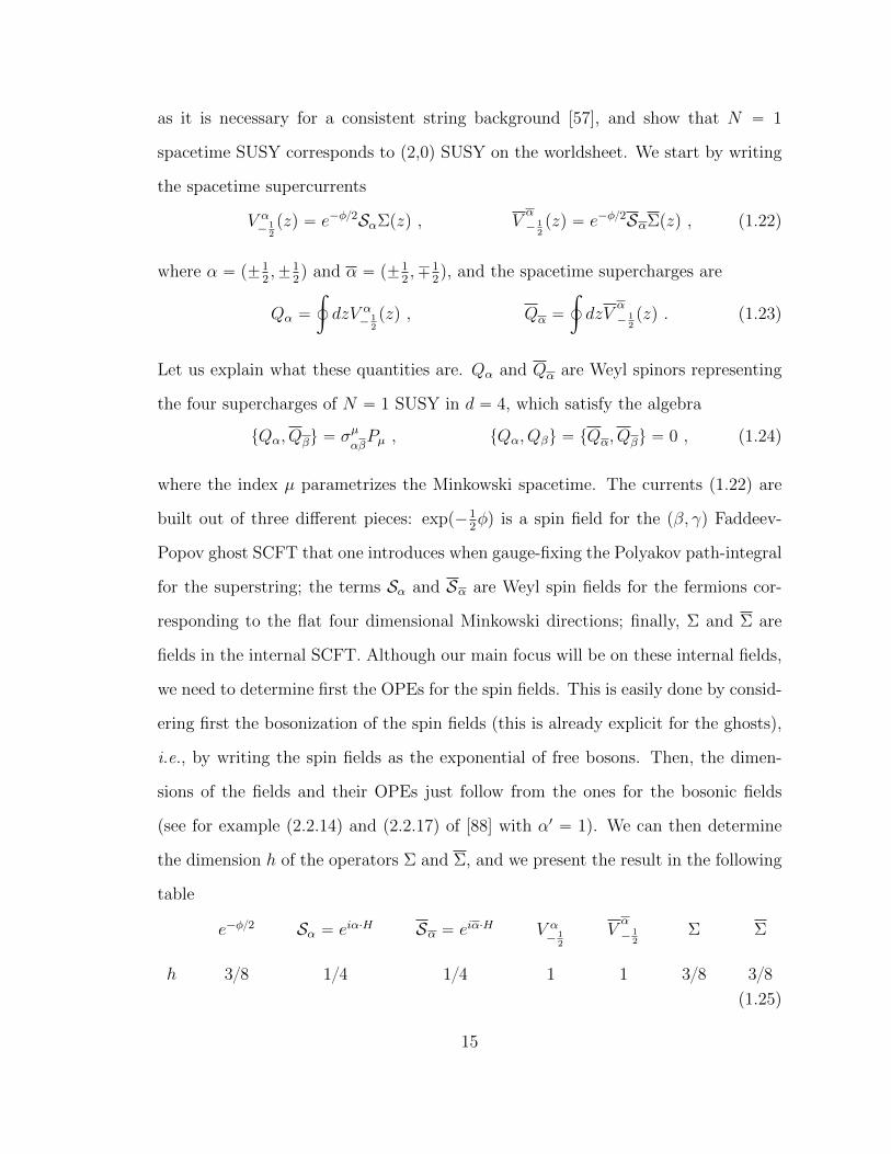
(see for example (2.2.14) and (2.2.17) of [88] with α1 “ 1). We can then determine
the dimension h of the operators Σ and Σ, and we present the result in the following
table
e´φ2 Sα “ eiα¨H Sα “ eiα¨H V α´ 1
2
Vα
´ 12
Σ Σ
h 38 14 14 1 1 38 38
(1.25)
15
The OPEs are
expp´1
2φqpzq expp´
1
2φqpwq „
expp´φq
pz ´ wq14,
SαSα „ σµαβψµpwq ,
SαSβ „ηαβI
pz ´ wq12, (1.26)
where I is the identity operator and similarly for Sα. Now, (1.24) determines the Σ
and Σ OPEs
ΣpzqΣpwq „ pz ´ wq34Opwq ` ¨ ¨ ¨ ,
ΣpzqΣpwq „ pz ´ wq34Opwq ` ¨ ¨ ¨ ,
ΣpzqΣpwq „I
pz ´ wq´34, (1.27)
where O and O are some dimension 3/2 operators. For example, the first equation
of (1.24) implies that
`
e´φ2SαΣ˘
pzq`
e´φ2SαΣ˘
pwq „expp´φq
pz ´ wq14σµαβψµpwqΣpzqΣpwq (1.28)
has a simple pole proportional to σµαβ
. The other two equations follow similarly by
imposing that the second set of equalities in (1.24) are satisfied.
At this point, we implement our assumption that we have already a N “ 1
SCFT on the worldsheet, that is, we have operators T pzq and Gpzq satisfying (1.12)
and (1.15) for c “ 9. A first result that will be useful later on comes from the
supersymmetry invariance of the gravitino vertex operator exppφqGpzq. In other
words`
e´φ2SαΣ˘
pzq`
eφG˘
pwq „ pz ´ wq12 expp12φqSαpwqΣpzqGpwq (1.29)
must have no single pole. This means that the most singular term in the OPEs
ΣpzqGpwq and ΣpzqGpwq must be proportional to pz ´ wq´12.
16
In order to study the next order in the ΣΣ OPE we consider the four-point
function
fpz1, z2, z3, z4q “ xΣpz1qΣpz2qΣpz3qΣpz4qy . (1.30)
The OPEs (1.27) and SLp2,Cq invariance constrain the above function to be
fpz1, z2, z3, z4q “
ˆ
z13z24
z12z14z23z34
˙34
. (1.31)
We can expand this expression as z12 Ñ 0 and we obtain
fpz1, z2, z3, z4q “ z´3412 z
´3434
„
1`3
4
z12z43
z23z24
` ¨ ¨ ¨
. (1.32)
The second order in the expansion signals the presence of an operator of dimension
´14` 2p38q “ 1 in the ΣΣ OPE
ΣpzqΣpwq „I
pz ´ wq´34` pz ´ wq14
1
2Jpwq , (1.33)
thus J is a up1q Kac-Moody current. In particular, we can see that Σ and Σ have
charge ˘32 under this symmetry
JpzqΣpwq „32Σpwq
z ´ w,
JpzqΣpwq „´32Σpwq
z ´ w. (1.34)
This is particularly nice, since we are starting to gain the structure of a more general
algebra. It is possible to implement the Sugawara decomposition described in the
previous section to all the operators we considered so far in the theory. In practice,
let us write Jpzq “ i?
3BHpzq, where Hpzq is a free scalar. From (1.34) we see that
Σ “ exppi?
32Hq and similarly Σ “ expp´i?
32Hq. For these there is no need
to multiply the exponential by a J-neutral operator because the dimensions already
17
work out. Instead, G does not have a definite charge under J , and we decompose it
as follows
G “ÿ
q
exppiq?
3HqGq0 . (1.35)
We can use these representations to determine for which values of q we are able to
reproduce the OPE between Σ and Σ with G. For example, in the case of ΣpzqGpwq
we find
´
exppi?
32HqΣ0
¯
pzq
˜
ÿ
q
exppiq?
3HqGq0
¸
pwq „ÿ
q
pz ´ wqq2 ¨ ¨ ¨ , (1.36)
from which we conclude that q “ ´1. The same analysis with Σ gives q “ 1, therefore
we have found a decomposition G “ 1?2pG``G´q analogous to (1.16), which satisfies
JpzqG˘pwq „˘G˘pwq
z ´ w. (1.37)
The above OPE can be rewritten as
GpwqJpzq „ ´1?
2
G`pwq ´G´pwq
z ´ w, (1.38)
that is pJ,´?
2G` `?
2G´q assemble in a primary N “ 1 superfield. It is then
convenient to define G ” 1?2pG`pwq ´G´pwqq which means that
GpzqGpwq „ ´12Jpwq
pz ´ wq2´
14BJpwq
z ´ w. (1.39)
For the last part of the argument it is convenient to expand the operators in modes
Gpzq “1
2
ÿ
r
Grz´r´32 , Gpzq “
1
2
ÿ
r
Grz´r´32 , Jpzq “
ÿ
n
Jnz´n´1 . (1.40)
These satisfy the relations
rJn, Jms “c
3mδm,´n, rJn, Grs “ Gn`r, rJn, Grs “ Gn`r, tGr, Gsu “ ps´ rqJr`s,
(1.41)
18
which follow from (1.18), (1.38) and (1.39). Now we compute
tGr, Gsu “ trJ0, Grs, Gsu “ J0GrGs ´GrJ0Gs `GsJ0Gr ´GsGrJ0
“ ´tGr, rJ0, Gssu ` rJ0, tGr, Gsus “ ´tGr, Gsu ´ pr ´ sqrJ0, Jr`ss
´ tGr, Gsu , (1.42)
which, translated back into the OPE language, yields
GpzqGpwq „ GpzqGpwq . (1.43)
This means that the GG and GG OPEs have the same singular terms. This fact
combined with (1.39) yield the remaining relations in (1.17). We have thus recovered
the structure of a N “ 2 superconformal algebra, proving the claim that N “ 1 SUSY
in spacetime implies (2,0) SUSY on the worldsheet.
1.4 Organization of the thesis
The remainder of this thesis is divided into three parts.
The work described in Chapter 2 is published in [27] and it was carried out in
collaboration with Ilarion Melnikov and Ronen Plesser. In this chapter we undertake
the study of hybrid theories with (2,2) supersymmetry. Roughly, a hybrid model is
a Landau-Ginzburg orbifold fibered non-trivially over a compact Kahler base. Al-
though the existence of such theories was known for more then two decades, their
properties have remained largely unexplored until recent years. In this work, we
present an intrinsic definition of a hybrid theory, that is independent of a GLSM
embedding. In order to do so, we derive several geometric constraints that charac-
terize the flow of the theory in the IR to a non-trivial fixed point. We also present
a method to compute the massless spectrum of the theory, which corresponds to
first-order deformations of the theory.
The work described in Chapter 3 is published in [26] and it was carried out in
collaboration with Ilarion Melnikov and Ronen Plesser. In this chapter we study
19
RG flows of (0,2) Landau-Ginzburg models. The superpotential of the UV theory
does not get renormalized under the RG flow, while the corrections to the kinetic
terms are believed to be irrelevant. This fact makes the problem very tractable,
as the IR behavior of the theory is encoded only in the superpotential. The UV
theory has in general a set of field redefinitions consistent with the symmetries of
the action, and the endpoints of RG flows corresponding to theories in the same
orbit of field redefinitions must coincide. If the UV superpotential admits a point
of enhanced symmetry, the R-symmetry at the conformal point might differ from
the naıve one of the UV theory for general values of the superpotential. This rather
simple observation has two striking consequences: first, the moduli space of the
theory is stratified according to basins of attraction of orbits of enhanced symmetry;
second, the conformal manifold describing a theory with the naıve UV properties
(central charges, etc.) might be empty. In this work, we study these “accidents” in
the context of (0,2) Landau-Ginzburg orbifolds, and, for a large subclass of theories,
we propose a geometric conjecture for the conformal manifold.
The work described in Chapter 4 is published in [25] and it was carried out in
collaboration with Ronen Plesser. In this chapter we undertake a study of α1 non-
perturbative corrections in the context of gauged-linear sigma models (GLSMs). It
is well known that, while most calculations are done in some appropriate large radius
limit (see for example the spectrum computation of Chapter 2), instanton effects are
important, as they can lift classically flat directions and they might destabilize the
vacuum and ruin conformal invariance. Indeed, at first it was thought that this was
the destiny of a general (0,2) model [35]. It was then shown that (0,2) models are non-
perturbatively stable when the gauge bundle splits non-trivially over every rational
curve in the Calabi-Yau [40]. Furthermore, there can be cases where the individual
instantons do contribute but these contributions sum up to zero [11]. It was argued in
the context of (0,2) GLSMs, that this is indeed the case [17]. However, the argument,
20
while elegant and powerful, was not fully exploited and the only concrete evidence
was based on a very simple example. In this work, we show that the argument does
not apply to all linear models, and we provide a counterexample. We then conclude
by proving a theorem that defines a class of linear models that are truly conformally
invariant.
21
2
(2,2) hybrid conformal field theories
2.1 Introduction
Just what is a hybrid anyway? In constructing two-dimensional superconformal field
theories (SCFTs) relevant for superstring vacua we are used to two sorts of massless
fluctuating fields: those corresponding to a non-linear sigma model (NLSM), and
those corresponding to a Landau-Ginzburg (LG) theory. The former define a clas-
sically conformally invariant system. Under favorable conditions, e.g. a Calabi-Yau
target space and world-sheet supersymmetry, the background fields can be chosen
to preserve superconformal invariance, and when the background is weakly coupled
in a “large radius limit” (i.e. the background fields have small gradients), the the-
ory reduces to a free-field limit. The latter have superpotential interactions that
explicitly break scale invariance; however, under favorable conditions, e.g. a quasi-
homogeneous superpotential, the IR limit of such a theory defines a non-trivial SCFT.
In each case, the utility of the description is two-fold: at a fundamental level, we
can use the weakly coupled UV theory to define a SCFT; as a practical matter, the
weakly coupled description, combined with non-renormalization theorems that follow
22
from supersymmetry, allow us to identify and compute certain protected quantities
such as chiral rings and massless spectra of the associated string vacua in terms of
the UV degrees of freedom.
By now the reader has surely guessed what is meant by a hybrid [97, 10]: it
is a two-dimensional theory that includes both types of massless fluctuating fields:
ones that have classically conformally invariant NLSM self-interactions, as well as
some that self-interact via a superpotential; of course an interesting hybrid also has
interactions between the two types of degrees of freedom. A hybrid is a fibered
theory, where the fiber is a LG theory with potential whose coefficients depend on
the fields of the base NLSM. The potential is chosen so that its critical point set is
the base target space. We then have two important questions: what are the criteria
for a hybrid theory to flow to a SCFT? how do we generalize NLSM/LG techniques
to compute physical quantities?
It is well-known that all of these descriptions— large radius limits of NLSMs,
Landau-Ginzburg orbifolds (LGOs), and hybrid loci—arise as phases of (2,2), and
more generally (0,2) gauged linear sigma models (GLSMs) [97]. The GLSM phi-
losophy is that each phase should yield a limiting locus where at least protected
quantities should be amenable to computation via the UV weakly-coupled field the-
ory description. Such techniques are known for large radius NLSM and LGO phases
but not for more general phases. In this work, we take a step in developing techniques
for what we will call the “good hybrid” phases of a GLSM.1
Although this does not cover a generic GLSM phase, and there are perhaps
good reasons [8] that we should not expect a simple description for a generic phase,
it does increase the set of special points in the moduli space amenable to exact
computations; this can lead to useful insights into stringy moduli space as in [11, 7,
1 Along the way we obtain a simple and direct description of the massless spectrum for the largeradius limit of a (0,2) NLSM — an application to CY NLSMs with non-standard embedding maybe found in appendix A.4 .
23
4, 28]. In addition, our definition of a good hybrid model, although inspired by the
GLSM construction, will not explicitly invoke the GLSM. Thus, we are in principle
providing a new class of UV theories that can lead to SCFTs without a known GLSM
embedding.
In this chapter we will focus on hybrid theories with (2,2) world-sheet supersym-
metry that are suitable for supersymmetric string compactification, i.e. ones with
integral Up1qLˆUp1qR R-symmetry charges; as in the case of LGO string vacua, this
is achieved by taking an appropriate orbifold.
While such models offer a good point of departure, it is clear that a more general
(0,2) hybrid framework will be both computationally useful and conceptually illu-
minating. While we are not going to tackle (0,2) hybrids in this thesis, for now we
note that just like (2,2) LG models, the hybrids incorporate a class of Lagrangian
deformations away from the (2,2) locus. These are obtained by smoothly deforming
the (2,2) superpotential to a more general (0,2) form.
In what follows, we first give a broad geometric description of (2,2) hybrids,
construct a Lagrangian for a good hybrid model and study its symmetries. With
that basic structure in hand, we turn to a technique, valid in the large base volume
limit and generalizing the well-known (2,2) and (0,2) LGO results of [61, 41], to
compute the massless heterotic spectrum of a hybrid compactification. We then
apply the techniques to a number of examples and conclude with a brief discussion
of applications and further directions.
2.2 A geometric perspective
The geometric setting for our theory is a (2,2) NLSM constructed with (2,2) chiral
superfields. Consider a Kahler manifold Y0 equipped with a holomorphic function—
the superpotential W—chosen so that its critical point set is a compact subset B Ă
Y0. More precisely, dW , a holomorphic section of the cotangent bundle T ˚Y0 , has
24
the property that dW´1p0q “ B Ă Y0. We call this the potential condition. A LG
model, with Y0 » Cn and B being the origin, is a familiar example. A compact Y0
necessarily has a trivial superpotential, and the resulting theory is just a standard
compact NLSM.
We say a geometry satisfying the potential condition has a hybrid model iff the
local geometry for B Ă Y0 can be modeled by Y — the total space of a rank n
holomorphic vector bundle X Ñ B over a compact smooth Kahler base B of complex
dimension d. The point of this definition is that the superpotential interactions will
lead to a suppression of finite fluctuations of fields away from B, so that the low
energy physics of the original NLSM will be well-approximated by the restriction
to the hybrid model. Our main task will be to describe this low energy physics,
and in what follows we will concentrate on the hybrid model geometry Y . In many
examples (e.g. the LG theories) Y » Y0, but our results apply to the more general
situation where Y is simply a local model. A simple example of a hybrid geometry,
where X “ Op´2q over B “ P1, is presented in appendix A.1.
In order to be reasonably confident that the low energy limit of a hybrid model
is a (2,2) SCFT, we will need the geometry to satisfy several additional conditions
intimately related to the existence of chiral symmetries and GSO projections. It will
be easiest to discuss these after we introduce the explicit Lagrangian realization of
this geometry. In our examples these features will already be present in the “UV”
completion of the hybrid model, offered either by Y0 or some other high energy
description such as a GLSM.2
A final geometric comment, relevant for heterotic applications, concerns (0,2)-
preserving deformations of these theories. (2,2) theories often admit a class of smooth
(0,2) deformations, where the left-moving fermions couple to a vector bundle E Ñ Y ,
a deformation of TY , and the (0,2) superpotential is encoded by a holomorphic section
2 It would be interesting to find hybrid examples where these features emerge accidentally.
25
J P ΓpE˚q with J´1p0q “ B. In the hybrid case there exist (0,2) deformations where
E “ TY but dJ ‰ 0; such a (0,2) superpotential cannot be integrated to a (2,2)
superpotential W . Turning these on leads to a simple class of (0,2) hybrid models.
2.3 Action and symmetries
In this section we construct the (2,2) SUSY UV action for a hybrid model and
analyze its symmetries. We begin with the necessary superspace formalism for a
flat Euclidean world-sheet with coordinates pz, zq. Since we are interested in (0,2)
deformations of (2,2) theories, it will be convenient for us to work with both (2,2) and
(0,2) superspaces.3 Let’s start with the latter. Introducing Grassmann coordinates
θ and θ, we obtain the supercharges
Q “ ´ BBθ` θBz, Q “ ´ B
Bθ` θBz, (2.1)
where Bz ” BBz. These form a representation of the (0,2) SUSY algebra: Q2 “
Q2“ 0 and tQ,Qu “ ´2Bz. The supercharges are graded by a Up1qR symmetry that
assigns charge q “ 1 to θ, and they anticommute with the supercovariant derivatives
D “ B
Bθ` θBz, D “ B
Bθ` θBz, (2.2)
that satisfy D2 “ D2“ 0 and tD,Du “ 2Bz.
To build a (2,2) superspace we introduce additional Grassmann variables θ1, θ1
and form Q1, Q1, as well as D1 and D1, by replacing pθ, θ, Bzq Ñ pθ1, θ1, Bzq, where
Bz “ BBz. These supercharges and derivatives are graded by Up1qL that assigns
charge q “ 1 to θ1.
2.3.1 Multiplets
We are interested in Kahler hybrid models with target space Y , and these can be
constructed by using bosonic chiral (2,2) superfields and their conjugate anti-chiral
3 Our superspace conventions are those of [81]; more details may be found in [39] or [95].
26
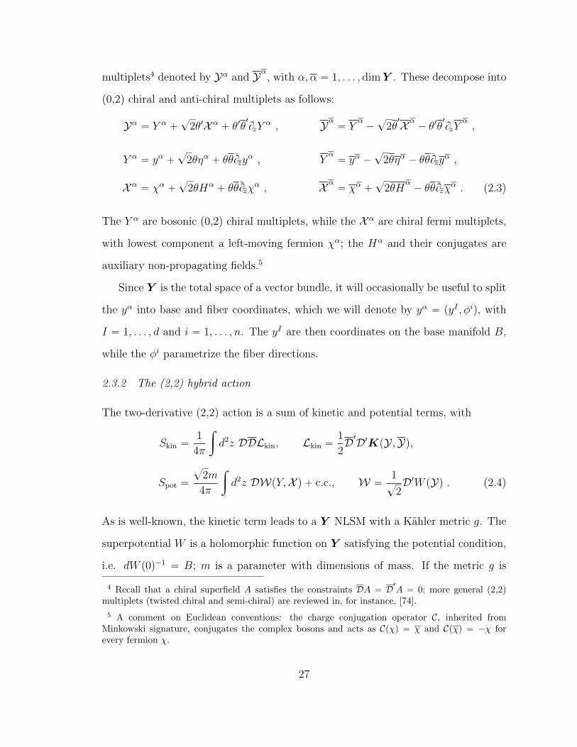
multiplets4 denoted by Yα and Yα, with α, α “ 1, . . . , dimY . These decompose into
(0,2) chiral and anti-chiral multiplets as follows:
Yα “ Y α`?
2θ1X α` θ1θ
1BzY
α , Yα “ Yα´?
2θ1X α
´ θ1θ1BzY
α,
Y α“ yα `
?2θηα ` θθBzy
α , Yα“ yα ´
?2θηα ´ θθBzy
α ,
X α“ χα `
?2θHα
` θθBzχα , X α
“ χα `?
2θHα´ θθBzχ
α . (2.3)
The Y α are bosonic (0,2) chiral multiplets, while the X α are chiral fermi multiplets,
with lowest component a left-moving fermion χα; the Hα and their conjugates are
auxiliary non-propagating fields.5
Since Y is the total space of a vector bundle, it will occasionally be useful to split
the yα into base and fiber coordinates, which we will denote by yα “ pyI , φiq, with
I “ 1, . . . , d and i “ 1, . . . , n. The yI are then coordinates on the base manifold B,
while the φi parametrize the fiber directions.
2.3.2 The (2,2) hybrid action
The two-derivative (2,2) action is a sum of kinetic and potential terms, with
Skin “1
4π
ż
d2z DDLkin, Lkin “1
2D1D1KpY ,Yq,
Spot “
?2m
4π
ż
d2z DWpY,X q ` c.c., W “1?
2D1W pYq . (2.4)
As is well-known, the kinetic term leads to a Y NLSM with a Kahler metric g. The
superpotential W is a holomorphic function on Y satisfying the potential condition,
i.e. dW p0q´1 “ B; m is a parameter with dimensions of mass. If the metric g is
4 Recall that a chiral superfield A satisfies the constraints DA “ D1A “ 0; more general (2,2)multiplets (twisted chiral and semi-chiral) are reviewed in, for instance, [74].
5 A comment on Euclidean conventions: the charge conjugation operator C, inherited fromMinkowski signature, conjugates the complex bosons and acts as Cpχq “ χ and Cpχq “ ´χ forevery fermion χ.
27
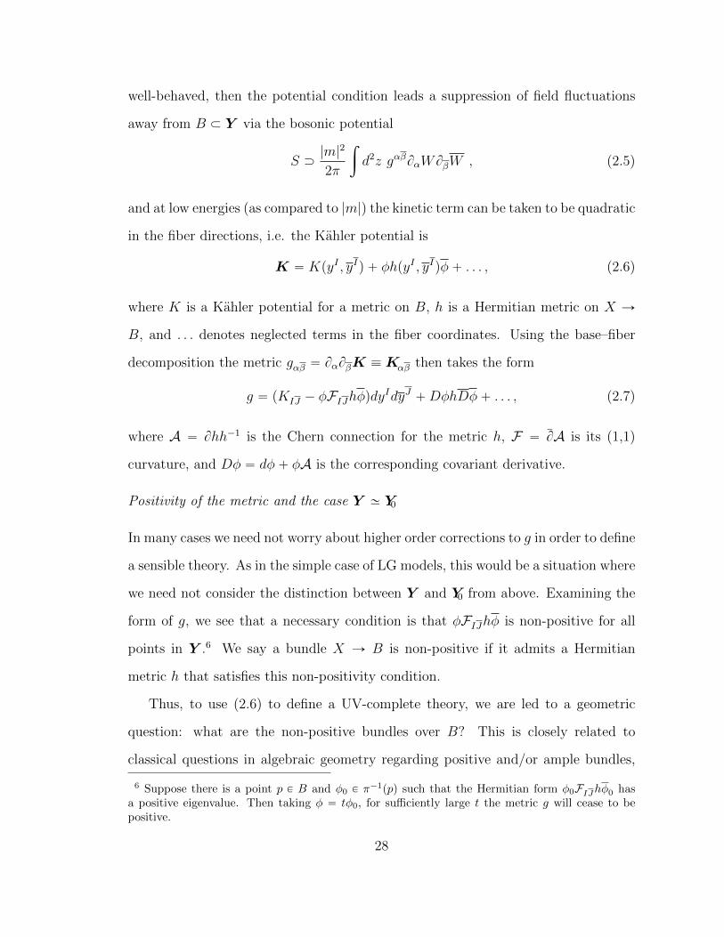
well-behaved, then the potential condition leads a suppression of field fluctuations
away from B Ă Y via the bosonic potential
S Ą|m|2
2π
ż
d2z gαβBαWBβW , (2.5)
and at low energies (as compared to |m|) the kinetic term can be taken to be quadratic
in the fiber directions, i.e. the Kahler potential is
K “ KpyI , yIq ` φhpyI , yIqφ` . . . , (2.6)
where K is a Kahler potential for a metric on B, h is a Hermitian metric on X Ñ
B, and . . . denotes neglected terms in the fiber coordinates. Using the base–fiber
decomposition the metric gαβ “ BαBβK ”Kαβ then takes the form
g “ pKIJ ´ φFIJhφqdyIdyJ `DφhDφ` . . . , (2.7)
where A “ Bhh´1 is the Chern connection for the metric h, F “ BA is its (1,1)
curvature, and Dφ “ dφ` φA is the corresponding covariant derivative.
Positivity of the metric and the case Y » Y0
In many cases we need not worry about higher order corrections to g in order to define
a sensible theory. As in the simple case of LG models, this would be a situation where
we need not consider the distinction between Y and Y0 from above. Examining the
form of g, we see that a necessary condition is that φFIJhφ is non-positive for all
points in Y .6 We say a bundle X Ñ B is non-positive if it admits a Hermitian
metric h that satisfies this non-positivity condition.
Thus, to use (2.6) to define a UV-complete theory, we are led to a geometric
question: what are the non-positive bundles over B? This is closely related to
classical questions in algebraic geometry regarding positive and/or ample bundles,
6 Suppose there is a point p P B and φ0 P π´1ppq such that the Hermitian form φ0FIJhφ0 has
a positive eigenvalue. Then taking φ “ tφ0, for sufficiently large t the metric g will cease to bepositive.
28
and using those classical results we can easily find sufficient conditions for non-
positivity. Recall that a line bundle LÑ B is said to be positive if its (1,1) curvature
form is positive; it is said to be negative if the dual bundle L˚ is positive [54, 73].
Taking X “ ‘iLi, a sum of negative and trivial line bundles, leads to many examples
of non-positive bundles.
We should stress two points: first, even this set of examples leads to many pre-
viously unexplored SCFTs. Second, more generally, we do not need to assume that
Y » Y0 or that g has no higher-order terms in the fibers. The low energy limit of a
UV theory with a hybrid model will be well-described by our action, and the poten-
tial condition will imply that the fiber corrections to the metric will not be important
to the low energy physics. We will analyze one such example below, where X is a
sum of a positive and a negative bundle.
(0,2) action
Since we are interested in heterotic applications as well as (0,2) deformations, it is
useful to have the manifestly (0,2) supersymmetric action obtained by integrating
over θ1, θ1
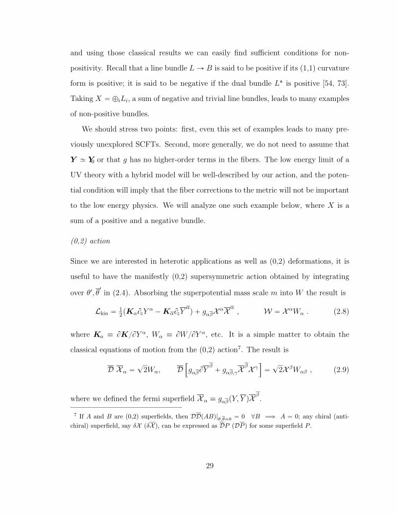
in (2.4). Absorbing the superpotential mass scale m into W the result is
Lkin “12pKαBzY
α´KαBzY
αq ` gαβX αX α
, W “ X αWα . (2.8)
where Kα ” BKBY α, Wα ” BW BY α, etc. It is a simple matter to obtain the
classical equations of motion from the (0,2) action7. The result is
D X α “?
2Wα, D”
gαβBYβ` gαβ,γX
βX γı
“?
2X βWαβ , (2.9)
where we defined the fermi superfield X α ” gαβpY, Y qXβ.
7 If A and B are (0,2) superfields, then DDpABq|θ,θ“0 “ 0 @B ùñ A “ 0; any chiral (anti-
chiral) superfield, say δX (δX ), can be expressed as DP (DP ) for some superfield P .
29
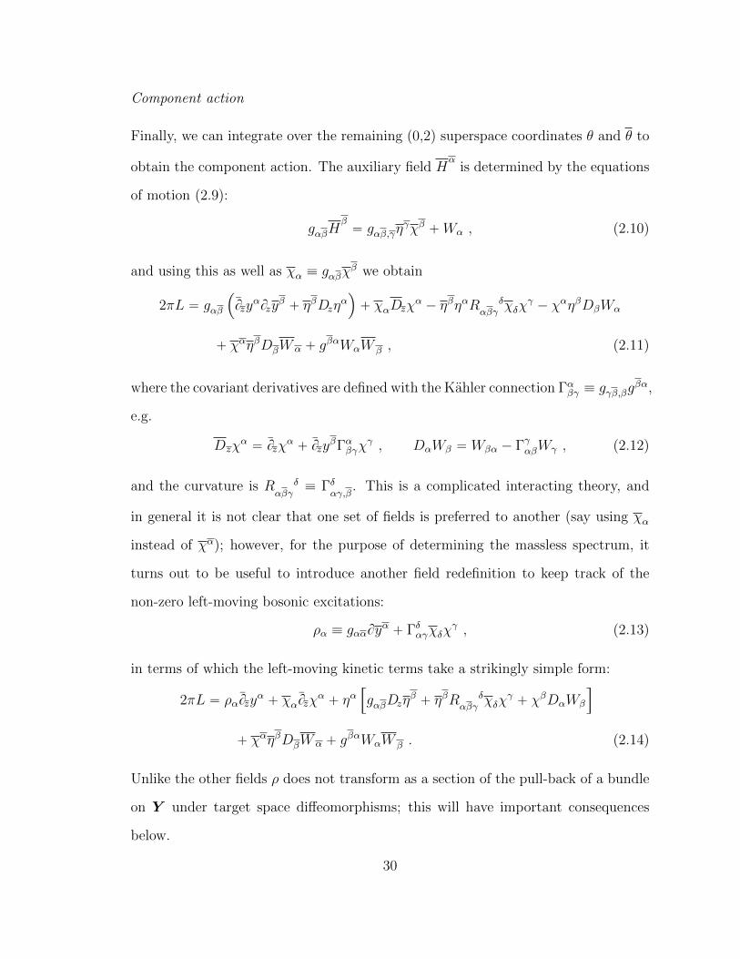
Component action
Finally, we can integrate over the remaining (0,2) superspace coordinates θ and θ to
obtain the component action. The auxiliary field Hα
is determined by the equations
of motion (2.9):
gαβHβ“ gαβ,γη
γχβ `Wα , (2.10)
and using this as well as χα ” gαβχβ we obtain
2πL “ gαβ
´
BzyαBzy
β` ηβDzη
α¯
` χαDzχα´ ηβηαR δ
αβγχδχ
γ´ χαηβDβWα
` χαηβDβWα ` gβαWαW β , (2.11)
where the covariant derivatives are defined with the Kahler connection Γαβγ ” gγβ,βgβα,
e.g.
Dzχα“ Bzχ
α` Bzy
βΓαβγχγ , DαWβ “ Wβα ´ ΓγαβWγ , (2.12)
and the curvature is R δαβγ
” Γδαγ,β
. This is a complicated interacting theory, and
in general it is not clear that one set of fields is preferred to another (say using χα
instead of χα); however, for the purpose of determining the massless spectrum, it
turns out to be useful to introduce another field redefinition to keep track of the
non-zero left-moving bosonic excitations:
ρα ” gααByα` Γδαγχδχ
γ , (2.13)
in terms of which the left-moving kinetic terms take a strikingly simple form:
2πL “ ραBzyα` χαBzχ
α` ηα
”
gαβDzηβ` ηβR δ
αβγχδχ
γ` χβDαWβ
ı
` χαηβDβWα ` gβαWαW β . (2.14)
Unlike the other fields ρ does not transform as a section of the pull-back of a bundle
on Y under target space diffeomorphisms; this will have important consequences
below.
30
2.3.3 Symmetries
We now examine the symmetries of the hybrid Lagrangian.
The Q supercharge
Our action respects (2,2) SUSY generated by the superspace operators Q and Q, as
well as their left-moving images. We define the action of the corresponding operators
Q and Q by
?2rξQ` ξQ, As ” ´ξQA´ ξQA, (2.15)
where ξ is an anti-commuting parameter and A is any superfield. In order to avoid
writing the graded commutator, we will use a condensed notation ξQ ¨A ” rξQ, As.
For our subsequent study of the right-moving Ramond ground states, we will be
particularly interested in the action of Q. Using the superfields in (2.3), we obtain
Q ¨ yα “ 0, Q ¨ χα “ 0, Q ¨ ηα “ Bzyα , Q ¨Hα
“ Bzχα ,
Q ¨ yα “ ´ηα , Q ¨ χα “ Hα, Q ¨ ηα “ 0 , Q ¨H
α“ 0 . (2.16)
The action of the remaining supercharges is easily obtained from this one by conju-
gation and/or switching left- and right-moving fermions. Eliminating the auxiliary
fields by their equations of motion we obtain
Q ¨ yα “ 0 , Q ¨ χα “ 0 , Q ¨ ηα “ Bzyα ,
Q ¨ yα “ ´ηα , Q ¨ χα “ Wα , Q ¨ ηα “ 0 . (2.17)
From (2.9) it follows that up to the η equations of motion we also have Q ¨ ρα “
χβWβα. Hence we can decompose Q as Q “ Q0 `QW , where the non-trivial action
is
Q0 ¨ yα“ ´ηα , Q0 ¨ η
α“ Bzy
α , QW ¨ χα “ Wα , QW ¨ ρα “ χβWβα . (2.18)
31
These satisfy Q2
0 “ Q2
W “ tQ0,QW u “ 0.8 Q0 is the supercharge for the NLSM
with W “ 0, while QW incorporates the effect of a non-trivial potential.
Chiral Up1q symmetries
The Up1qL ˆ Up1qR symmetries play an important role in relating the UV hybrid
model to the IR physics of the corresponding SCFT. In the classical NLSM with
W “ 0 the presence of these symmetries is a consequence of the existence of an
integrable, metric-compatible complex structure on Y . In terms of component fields,
the symmetries leave the bosonic fields invariant, while rotating the fermions as
follows:
Up1q0L : δ0Lη “ 0, δ0
Lχ “ ´iεχ ; Up1q0R : δ0Rη “ ´iεη, δ0
Rχ “ 0 , (2.19)
where ε is an infinitesimal real parameter. These naive symmetries are explicitly
broken by the superpotential, but they can be improved if the geometry pY , gq
admits a holomorphic Killing vector V satisfying LVW “ W .9 V generates a non-
chiral symmetry action
δV Yα“ iεV α
pY q, δV Yα“ ´iεV
αpY q; δVX α
“ iεV α,βX β , δVX
α“ ´iεV
α
,βXβ,
(2.20)
and it is easy to see that δL,R ” δ0L,R ` δV are symmetries of the classical action.
While Up1qdiag Ă Up1qL ˆ Up1qR has a non-chiral action on the fermions and
hence is non-anomalous, Up1qL is a chiral symmetry that will be anomaly free iff
c1pTY q “ 0, a condition satisfied when Y is a non-compact Calabi-Yau manifold, i.e.
8 If we keep the terms in Q ¨ ρ proportional to η equations of motion and decompose that intoa W -independent and W -dependent contributions, we find that the decomposition Q “ Q0 `QW
into a pair of nilpotent anti-commuting operators holds without use of equations of motion; for usthe result of (2.18) will be sufficient.
9 Holomorphic Killing vectors satisfy V α,β“ 0 and LV g “ 0. They are a familiar topic in
supersymmetry—see, e.g., Appendix D of [94]. Note that on a compact Kahler manifold a Killingvector field is holomorphic, but this can fail on a non-compact manifold. Killing vectors on Kahlermanifolds are further discussed in [14, 83].
32
Y has a trivial canonical bundle KY » OY . In what follows we assume KY is indeed
trivial (this is stronger than c1pTY q “ 0). When X “ ‘iLi, a sum of line bundles
such that biLi is negative, then since KY “ KB bi L˚i the anti-canonical class of B
is very ample and B is Fano.10
In what follows we will denote the conserved charge for Up1qL (Up1qR) by J0 (J0)
and its eigenvalues on various operators and states by q (q).
R-symmetries for good hybrid models
We would like to identify the UV Up1qL ˆ Up1qR symmetries described above with
their counterparts in the conjectured IR SCFT. As usual, there is a small subtlety in
doing this when V is not unique. In practice this is easily achieved by picking a suffi-
ciently generic superpotential and more generally, one could use c-extremization [23]
to fix Up1qL ˆ Up1qR up to the usual caveats of accidental IR symmetries.
More importantly, in order for the UV R-symmetry of the hybrid model to be a
good guide to the IR physics, we need V to be a vertical vector field, i.e. LV π˚pωq “ 0
for all forms ω P Ω‚pBq, and in particular the Up1qLˆUp1qR symmetries fix B point-
wise. We denote a model where this is the case a good hybrid. As we show in
Appendix A.2 this implies
V “řni“1qiφ
i BBφi` c.c. (2.21)
for some real charges qi. The qi have to be compatible with the transition functions
definingX Ñ B, and since LVW “ W , andW is polynomial in every patch, qi P Qě0.
In a LG theory, i.e B a point, standard results show that if the potential condition
is satisfied then without loss of generality 0 ă qi ď 12 [69, 67]. More generally,
the potential condition requires that W pyI , φq, thought of locally as a LG potential
for the fiber fields φ depending on the “parameters” yI , should be non-singular in a
10 A variety is Fano iff its anti-canonical class is ample; Fano varieties are quite special: for instanceHipB,Oq “ 0 for i ą 0, PicpBq » H2pB,Zq; in addition, they are classified in dimension d ď 3 andadmit powerful criteria for evaluating positivity of bundles [73].
33
small neighborhood of any generic point in B. Hence, the range of allowed qi is the
same for a hybrid theory as it is for LG models.
The orbifold action
Our main interest in the hybrid SCFTs is for applications to supersymmetric com-
pactification of type II or heterotic string theories. For left-right symmetric theories
this requires the existence of Up1qL ˆ Up1qR symmetries with integral q, q charges
of all (NS,NS) sector states [15]. Our hybrid theory, if it flows as expected to a
c “ c “ 9 SCFT in the IR will not satisfy this condition. Fortunately, the solution
is the same as it is for Gepner models [51] or LG orbifolds [92, 58]: we gauge the
discrete symmetry Γ generated by expr2πiJ0s, where J0 denotes the conserved Up1qL
charge; since all fields have q´q P Z, the orbifold by Γ is sufficient to obtain integral
charges.
In the line bundle case with qi “ nidi we then see that Γ » ZN , with N the least
common multiple of pd1, . . . , dnq. Since Γ is embedded in a continuous non-anomalous
symmetry we expect the resulting orbifold to be a well-defined quantum field theory,
and the resulting orbifold SCFT will be suitable for a string compactification.
In addition to the introduction of twisted sectors and the projection, the orbifold
has one important consequence for the physics of hybrid models: it allows us to
consider more general “orbi-bundles,” where the fiber in X Ñ B is of the form CnΓ,
and the transition functions are defined up to the orbifold action. For instance, we
will examine a theory with B “ P3 and X “ Op´52q‘Op´32q, where the orbifold
Γ “ Z2 reflects both of the fiber coordinates.11
11 A GLSM embedding of this hybrid model is given in section 2.5 of [1] .
34
2.3.4 The quantum theory and the hybrid limit
Having defined the classical hybrid model’s Lagrangian and discussed its symmetries,
we now discuss the quantum theory. To orient ourselves in the issues involved, let’s
recall the case of (2,2) LG models — the simplest examples of hybrids. These theories
have a Lagrangian description at some renormalization scale µ as a free kinetic term
for chiral multiplets, and a superpotential interaction with dimensionful couplings
m. The theory is weakly coupled when µ " m, and we can use the Lagrangian
and (approximately) free fields to describe the theory. The low energy limit µ Ñ 0
is then strongly coupled, and while W is protected by SUSY non-renormalization
theorems, the kinetic term receives a complicated but irrelevant set of corrections.
There is by now overwhelming evidence that these do flow to the expected SCFTs,
in accordance with the original proposals [75, 93], and computations of RG-invariant
quantities allow us to use the weakly coupled µ " m description to describe exactly
the SCFT’s (c,c) chiral ring and more generally the Q-cohomology. Furthermore,
the results extend to LGOs suitable for string compactification.12
There is a small IR subtlety in using the weakly coupled LG description: the
theory at W “ 0 is non-compact and has all the usual difficulties associated with
non-compact bosons. This is of course not very subtle since the theory is free;
however, more to the point, in using the weakly coupled description we still keep
track of the R-charges and weights that follow from the superpotential and do not
consider states supported away from the W “ 0 locus.
A more general hybrid theory has a similar structure, except that now there are
two sorts of couplings: the superpotential couplings mµ, as well as the choice of
Kahler class on the base B. Although the latter coupling is typically encoded in
the kinetic D-term, it can also be expressed as a deformation of the twisted chiral
12 These typically have non-trivial (a,c) rings encoded in the twisted sectors, and that ring structureis not easy to access directly via the LG orbifold description.
35
superpotential. Hence, the Kahler class and superpotential couplings do not receive
quantum corrections. Of course we do expect corrections to the D-terms, but these
should be irrelevant just as they are in the LG case. Moreover, there is good evidence,
based on GLSM constructions, that the hybrid models with a GLSM UV completion
should flow to SCFTs with expected properties (i.e. correct central charges and R-
symmetries), and we expect the same to hold for more general hybrid models. As
in the LG case, the strict W “ 0 limit may be subtle, perhaps even more so, since
it may require us to specify additional details about the geometry of Y . However,
we may use the same cure for these IR subtleties as we do in the LG case: use the
R-charges and weights encoded by the superpotential and restrict attention to field
configurations and states supported on B.
Assuming a hybrid model does flow to an expected SCFT, we would like to
have techniques to evaluate RG-invariant quantities such as the Q-cohomology. It
is here that there will be important conceptual and technical differences from the
LG case due to the non-trivial base geometry B. For instance, we expect the Q-
cohomology to depend on the choice of Kahler class on B. While there will not
be a perturbative dependence, we do in general expect corrections from world-sheet
instantons wrapping non-trivial cycles in B. These corrections are suppressed when
B is large, which leads us to define the hybrid analogue of the large radius limit of a
NLSM: the hybrid limit, where the Kahler class of B is taken to be arbitrarily deep
in its Kahler cone. In what follows, we will study the Q-cohomology of a hybrid
model in the hybrid limit.
2.4 Massless spectrum of heterotic hybrids
In this section we develop techniques to evaluate the massless spectrum for a com-
pactification of the E8ˆE8 heterotic string based on a c “ c “ 9 (2,2) hybrid SCFT.13
13 The SOp32q case can be handled in an entirely analogous fashion.
36
We first review the standard prescription [51, 92, 61] to obtain a modular invariant
theory and identify world-sheet Ramond ground states with massless fermions in
spacetime. We then discuss how to enumerate these ground states by studying the
Q cohomology in the hybrid limit.
2.4.1 Spacetime generalities
In order to describe a heterotic string compactification, we complete our hybrid
c “ c “ 9 N “ p2, 2q SCFT internal theory to a critical heterotic theory by adding
ten left-moving fermions (with fermion number Fλ) that realize an sop10q level 1
current algebra, a left-moving level 1 hidden e8 current algebra, and the free c “ 4,
c “ 6 theory of the uncompactified spacetime R1,3.
A modular invariant theory is obtained by performing left- and right- GSO pro-
jections. The left-moving GSO projection onto eiπJ0p´qFλ “ 1 is responsible for
enhancing the linearly realized up1qL ‘ sop10q gauge symmetry to the full e6. The
right-moving GSO projection has a similar action, combining J0 with the fermion
number of the R1,3 theory. Its immediate spacetime consequence is N “ 1 space-
time supersymmetry, or equivalently, a relation, via spectral flow, between states in
right-moving Neveu-Schwarz and Ramond sectors. Spacetime fermions arise in the
(NS,R) and (R,R) sectors, and supersymmetry allows us to identify the full spectrum
of supermultiplets in the spacetime theory from these states.
The spacetime theory obtained by this procedure will have a model-independent
set of massless fermions: the gauginos of the hidden e8, the gravitino, and the dilatino.
In what follows we focus on the model-dependent massless spectrum. In particular,
the hidden e8 degrees of freedom are always restricted to their NS ground state and
just make a contribution to the left-moving zero-point energy.
On-shell string states have vanishing left- and right-moving energies. For massless
states there is no contribution to L0 from the R1,3 free fields; massless fermions are
37
thus states in the (R,R) and (NS,R) sectors with vanishing left-moving and right-
moving energies. In the (R,R) sector, massless states are associated to the ground
states in the internal theory, related by spectral flow to (NS,NS) operators comprising
the “chiral rings” [93] of the theory. Massless states in the (NS,R) sector include
states related to these by left-moving spectral flow as well as additional states. The
main result of [61] is a method for describing these states in LGO theories, which we
here extend to hybrids. This relies on the familiar fact that since
tQ,Qu “ 2L0 ; Q2“ Q
2“ 0 (2.22)
the kernel of L0 is isomorphic to the cohomology of Q.
The right-moving GSO projection is onto states with q P Z ` 12; those with
q “ ´12 (q “ 12) correspond to chiral (anti-chiral) multiplets, while states with
q “ ˘32 are gauginos in vector multiplets. The Up1qL charge q determines the e6
representation according to the decomposition
e6 Ą sop10q ‘ up1q
78 “ 450 ‘ 16´32 ‘ 1632 ‘ 10
27 “ 1612 ‘ 10´1 ‘ 12
27 “ 16´12 ‘ 101 ‘ 1´2 . (2.23)
As in the LG orbifold case [92, 61], the GSO projection can be combined with the
hybrid orbifold of Γ “ ZN to an orbifold by Z2 ˙ ZN – Z2N . Therefore we need to
study the 2N sectors twisted by rexppiπJ0qsk, k “ 0, . . . , 2N ´ 1.14 Spacetime CPT
exchanges the k-th and the p2N ´ kq-th sectors, and CPT invariance means we can
restrict our analysis to the k “ 0, 1, . . . , N . sectors. The states arising in (R,R) (k
even) sectors give rise to e6-charged matter. This is easy to see since in this case the
ground states of the sop10q current algebra transform in 16‘16. Massless e6-singlets
14 That is, schematically, in the k-th twisted sector fields satisfy φpze2πi, ze´2πiq “
rexppiπJ0qskφpz, zq. We will make these periodicities more precise shortly.
38
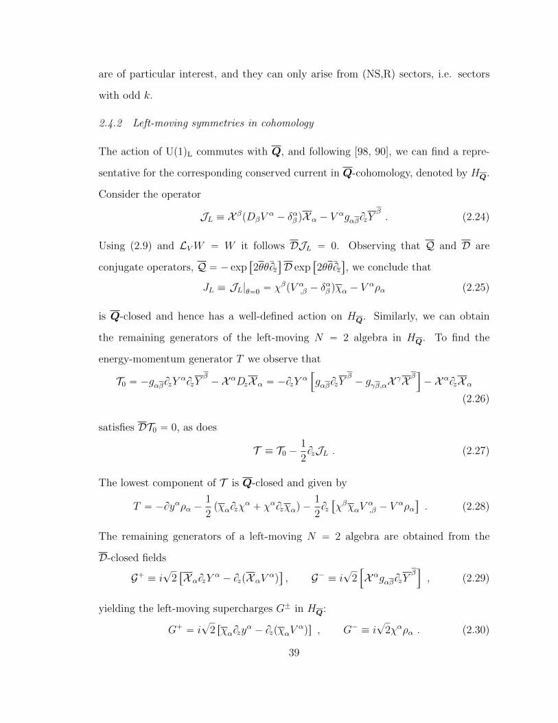
are of particular interest, and they can only arise from (NS,R) sectors, i.e. sectors
with odd k.
2.4.2 Left-moving symmetries in cohomology
The action of Up1qL commutes with Q, and following [98, 90], we can find a repre-
sentative for the corresponding conserved current in Q-cohomology, denoted by HQ.
Consider the operator
JL ” X βpDβV
α´ δαβ qX α ´ V
αgαβBzYβ. (2.24)
Using (2.9) and LVW “ W it follows DJL “ 0. Observing that Q and D are
conjugate operators, Q “ ´ exp“
2θθBz‰
D exp“
2θθBz‰
, we conclude that
JL ” JL|θ“0 “ χβpV α,β ´ δ
αβ qχα ´ V
αρα (2.25)
is Q-closed and hence has a well-defined action on HQ. Similarly, we can obtain
the remaining generators of the left-moving N “ 2 algebra in HQ. To find the
energy-momentum generator T we observe that
T0 “ ´gαβBzYαBzY
β´ X αDzX α “ ´BzY
α”
gαβBzYβ´ gγβ,αX γX β
ı
´ X αBzX α
(2.26)
satisfies DT0 “ 0, as does
T ” T0 ´1
2BzJL . (2.27)
The lowest component of T is Q-closed and given by
T “ ´Byαρα ´1
2pχαBzχ
α` χαBzχαq ´
1
2Bz“
χβχαVα,β ´ V
αρα‰
. (2.28)
The remaining generators of a left-moving N “ 2 algebra are obtained from the
D-closed fields
G` ” i?
2“
X αBzYα´ BzpX αV
αq‰
, G´ ” i?
2”
X αgαβBzYβı
, (2.29)
yielding the left-moving supercharges G˘ in HQ:
G` “ i?
2 rχαBzyα´ BzpχαV
αqs , G´ ” i
?2χαρα . (2.30)
39
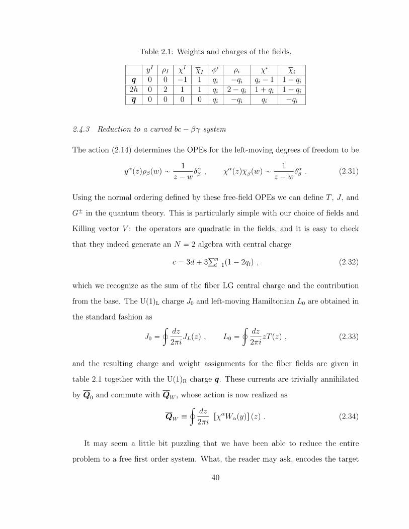
Table 2.1: Weights and charges of the fields.
yI ρI χI χI φi ρi χi χiq 0 0 ´1 1 qi ´qi qi ´ 1 1´ qi2h 0 2 1 1 qi 2´ qi 1` qi 1´ qiq 0 0 0 0 qi ´qi qi ´qi
2.4.3 Reduction to a curved bc´ βγ system
The action (2.14) determines the OPEs for the left-moving degrees of freedom to be
yαpzqρβpwq „1
z ´ wδαβ , χαpzqχβpwq „
1
z ´ wδαβ . (2.31)
Using the normal ordering defined by these free-field OPEs we can define T , J , and
G˘ in the quantum theory. This is particularly simple with our choice of fields and
Killing vector V : the operators are quadratic in the fields, and it is easy to check
that they indeed generate an N “ 2 algebra with central charge
c “ 3d` 3řni“1p1´ 2qiq , (2.32)
which we recognize as the sum of the fiber LG central charge and the contribution
from the base. The Up1qL charge J0 and left-moving Hamiltonian L0 are obtained in
the standard fashion as
J0 “
¿
dz
2πiJLpzq , L0 “
¿
dz
2πizT pzq , (2.33)
and the resulting charge and weight assignments for the fiber fields are given in
table 2.1 together with the Up1qR charge q. These currents are trivially annihilated
by Q0 and commute with QW , whose action is now realized as
QW ”
¿
dz
2πirχαWαpyqs pzq . (2.34)
It may seem a little bit puzzling that we have been able to reduce the entire
problem to a free first order system. What, the reader may ask, encodes the target
40
space geometry, for example? The answer, familiar from [85, 99], is that the free
field theory description only applies patch by patch in field-space. That is, we cover
Y with open sets Ua and local coordinates xαa , and on each Uab “ Ua X Ub ‰ H
xb “ xbpxaq, and we define the holomorphic transition functions
pTbaqαβ ”
BxαbBxβa
, pSbaqαβγ ” pT´1ba q
αδ pTbaq
δβ,γ . (2.35)
The left-moving fields then patch according to
yαb “ xαb pyaq , χαb “ pTbaqαβχ
βa , χbα “ pT
´1ba q
βαχaβ ,
ρbα “: pT´1ba q
βα
“
ρbβ ´ Sδbaβγχδχγ‰
: , (2.36)
where the transition functions are evaluated at ya, e.g. Tba “ Tbapyaq. Note that the
patching of ρ requires a normal-ordering due to singularities in the y ´ ρ and χ´ χ
OPEs. Of course there are similar transformations for the right-moving fields y and
η, η. For instance, the ηI transform as sections of y˚pTBq.15
These transition functions require a careful analysis when we expand about world-
sheet instanton configurations, i.e. non-trivial holomorphic maps Σ Ñ Y . This,
together with non-trivial fermi zero modes in the background of an instanton will
lead to world-sheet instanton corrections to Q0.16 These corrections vanish in the
hybrid limit where we expand about constant maps Bzy “ Bzy “ 0, and the only
non-trivial Q0 action is on the anti-holomorphic zero modes Q0 ¨ yα0 “ ´η
α0 . In fact,
since the ηı are Q-exact, as far as cohomology is concerned, we can safely ignore
the ηı as well as the anti-holomorphic bosonic fiber zero modes φı
0. So, the only
non-trivial Q0 action is on the base anti-holomorphic zero modes: Q0 ¨ yI0 “ ´η
I0. In
what follows we will drop the zero mode subscript on these right-moving fields with
the understanding that y and η will denote the base antiholomorphic zero modes.
15 As we are working on a flat world-sheet throughout this chapter, we do not keep track of theworld-sheet spinor properties of the fermionic degrees of freedom.
16 Since QW is associated to a chiral superpotential, we do not expect it to be corrected by world-sheet instantons.
41
2.4.4 Massless states in the hybrid limit
Our task now is to work out, in each twisted sector, the set of GSO-even states
that belong to HQ and carry left-moving energy E “ 0. We construct the relevant
states (i.e. the only ones with required energy and charges) in the Hilbert space
as polynomials in the fermions and non-zero bosonic oscillator modes tensored with
wavefunctions of the bosonic zero modes. In a generic twisted sector the bosonic
zero modes correspond to the compact base B, while in less generic sectors there can
be additional bosonic zero modes. However, since the non-compact bosonic modes
will be lifted by the superpotential, in what follows all bosonic wavefunctions will be
taken to be polynomial in the fiber fields.
The operators T and JL can be used to grade the states according to their energy
E and left-moving charge q, and we can evaluate Q-cohomology on the states of
fixed E and q. An important simplification comes from working in the right-moving
Ramond ground sector. A look at (2.18) shows that, as far as Q-cohomology is
concerned, we can neglect any states containing oscillators in Bzyα, as well as any
non-zero mode of ηα. We choose the Ramond ground state annihilated by the zero
modes of ηα, so our states will be constructed without ηα or right-moving bosonic
oscillators. We will call the resulting space of states the restricted Hilbert space H.
In general this will be infinite-dimensional even at fixed E and q.
Twisted modes and ground state quantum numbers
In this section we provide expressions for E, q and q of the states in a fixed twisted
sector. For simplicity, we work out the case X “ ‘iLi. The result extends imme-
diately to orbi-bundles of the form X “ ‘iLxii for xi P Q. It should be possible to
treat the case of more general X at the price of additional notation.
The first task is to describe the mode expansions of the fields and the quantum
numbers of the ground states |ky. While we can restrict to right-moving (i.e. anti-
42
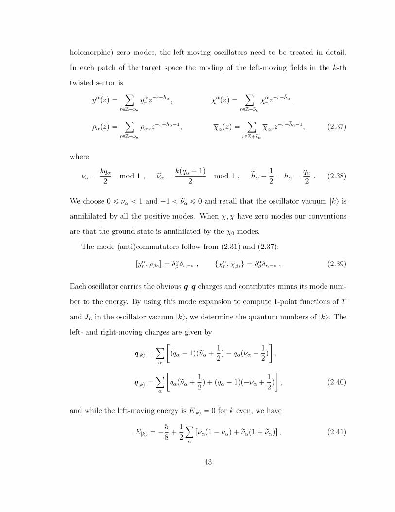
holomorphic) zero modes, the left-moving oscillators need to be treated in detail.
In each patch of the target space the moding of the left-moving fields in the k-th
twisted sector is
yαpzq “ÿ
rPZ´να
yαr z´r´hα , χαpzq “
ÿ
rPZ´rνα
χαr z´r´rhα ,
ραpzq “ÿ
rPZ`να
ραrz´r`hα´1, χαpzq “
ÿ
rPZ`rνα
χαrz´r`rhα´1, (2.37)
where
να “kqα2
mod 1 , rνα “kpqα ´ 1q
2mod 1 , rhα ´
1
2“ hα “
qα2. (2.38)
We choose 0 ď να ă 1 and ´1 ă rνα ď 0 and recall that the oscillator vacuum |ky is
annihilated by all the positive modes. When χ, χ have zero modes our conventions
are that the ground state is annihilated by the χ0 modes.
The mode (anti)commutators follow from (2.31) and (2.37):
ryαr , ρβss “ δαβ δr,´s , tχαr , χβsu “ δαβ δr,´s . (2.39)
Each oscillator carries the obvious q, q charges and contributes minus its mode num-
ber to the energy. By using this mode expansion to compute 1-point functions of T
and JL in the oscillator vacuum |ky, we determine the quantum numbers of |ky. The
left- and right-moving charges are given by
q|ky “ÿ
α
„
pqα ´ 1qprνα `1
2q ´ qαpνα ´
1
2q
,
q|ky “ÿ
α
„
qαprνα `1
2q ` pqα ´ 1qp´να `
1
2q
, (2.40)
and while the left-moving energy is E|ky “ 0 for k even, we have
E|ky “ ´5
8`
1
2
ÿ
α
rναp1´ ναq ` rναp1` rναqs , (2.41)
43
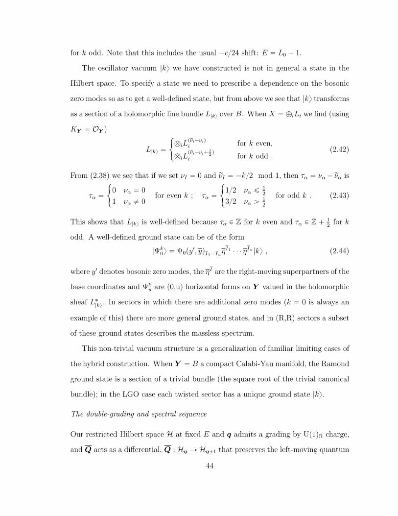
for k odd. Note that this includes the usual ´c24 shift: E “ L0 ´ 1.
The oscillator vacuum |ky we have constructed is not in general a state in the
Hilbert space. To specify a state we need to prescribe a dependence on the bosonic
zero modes so as to get a well-defined state, but from above we see that |ky transforms
as a section of a holomorphic line bundle L|ky over B. When X “ ‘iLi we find (using
KY “ OY )
L|ky “
#
biLprνi´νiqi for k even,
biLprνi´νi`
12q
i for k odd .(2.42)
From (2.38) we see that if we set νI “ 0 and rνI “ ´k2 mod 1, then τα “ να´ rνα is
τα “
#
0 να “ 0
1 να ‰ 0for even k ; τα “
#
12 να ď12
32 να ą12
for odd k . (2.43)
This shows that L|ky is well-defined because τα P Z for k even and τα P Z ` 12
for k
odd. A well-defined ground state can be of the form
|Ψk0y “ Ψ0py
1, yqI1¨¨¨IuηI1 ¨ ¨ ¨ ηIu |ky , (2.44)
where y1 denotes bosonic zero modes, the ηI are the right-moving superpartners of the
base coordinates and Ψku are (0,u) horizontal forms on Y valued in the holomorphic
sheaf L˚|ky. In sectors in which there are additional zero modes (k “ 0 is always an
example of this) there are more general ground states, and in (R,R) sectors a subset
of these ground states describes the massless spectrum.
This non-trivial vacuum structure is a generalization of familiar limiting cases of
the hybrid construction. When Y “ B a compact Calabi-Yau manifold, the Ramond
ground state is a section of a trivial bundle (the square root of the trivial canonical
bundle); in the LGO case each twisted sector has a unique ground state |ky.
The double-grading and spectral sequence
Our restricted Hilbert space H at fixed E and q admits a grading by Up1qR charge,
and Q acts as a differential, Q : Hq Ñ Hq`1 that preserves the left-moving quantum
44
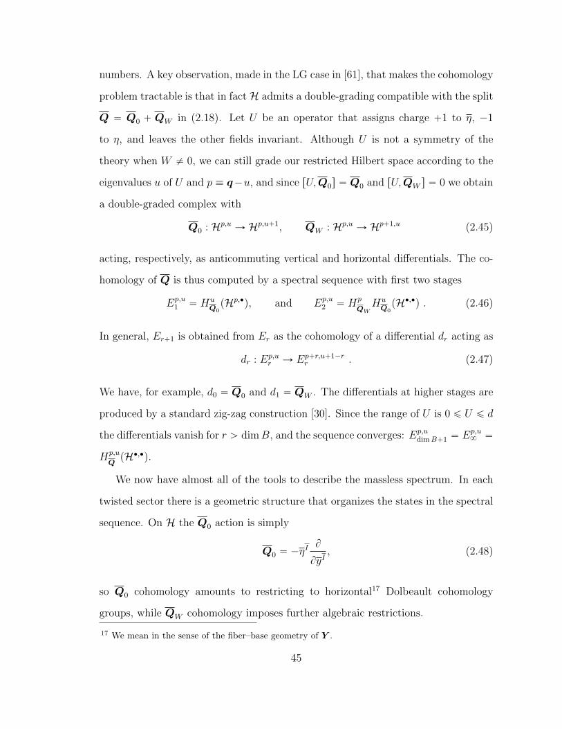
numbers. A key observation, made in the LG case in [61], that makes the cohomology
problem tractable is that in factH admits a double-grading compatible with the split
Q “ Q0 ` QW in (2.18). Let U be an operator that assigns charge `1 to η, ´1
to η, and leaves the other fields invariant. Although U is not a symmetry of the
theory when W ‰ 0, we can still grade our restricted Hilbert space according to the
eigenvalues u of U and p ” q´u, and since rU,Q0s “ Q0 and rU,QW s “ 0 we obtain
a double-graded complex with
Q0 : Hp,uÑ Hp,u`1, QW : Hp,u
Ñ Hp`1,u (2.45)
acting, respectively, as anticommuting vertical and horizontal differentials. The co-
homology of Q is thus computed by a spectral sequence with first two stages
Ep,u1 “ Hu
Q0pHp,‚
q, and Ep,u2 “ Hp
QWHu
Q0pH‚,‚q . (2.46)
In general, Er`1 is obtained from Er as the cohomology of a differential dr acting as
dr : Ep,ur Ñ Ep`r,u`1´r
r . (2.47)
We have, for example, d0 “ Q0 and d1 “ QW . The differentials at higher stages are
produced by a standard zig-zag construction [30]. Since the range of U is 0 ď U ď d
the differentials vanish for r ą dimB, and the sequence converges: Ep,udimB`1 “ Ep,u
8 “
Hp,u
QpH‚,‚q.
We now have almost all of the tools to describe the massless spectrum. In each
twisted sector there is a geometric structure that organizes the states in the spectral
sequence. On H the Q0 action is simply
Q0 “ ´ηI B
ByI, (2.48)
so Q0 cohomology amounts to restricting to horizontal17 Dolbeault cohomology
groups, while QW cohomology imposes further algebraic restrictions.
17 We mean in the sense of the fiber–base geometry of Y .
45
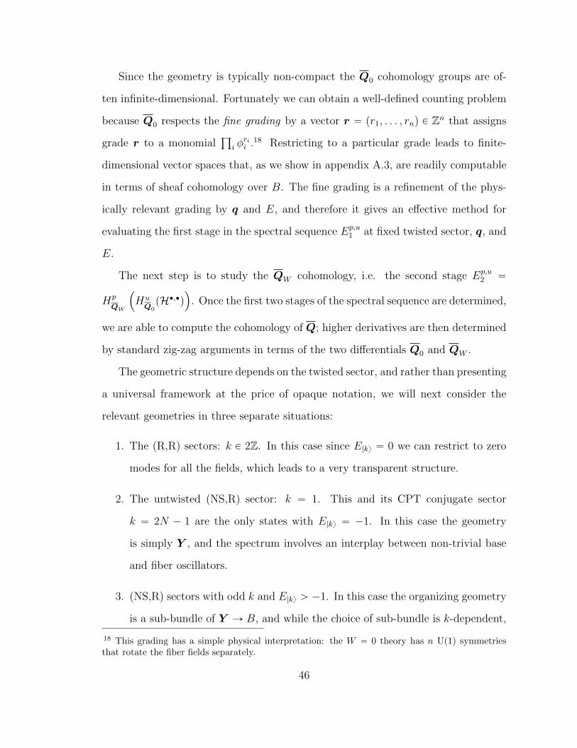
Since the geometry is typically non-compact the Q0 cohomology groups are of-
ten infinite-dimensional. Fortunately we can obtain a well-defined counting problem
because Q0 respects the fine grading by a vector r “ pr1, . . . , rnq P Zn that assigns
grade r to a monomialś
i φrii .18 Restricting to a particular grade leads to finite-
dimensional vector spaces that, as we show in appendix A.3, are readily computable
in terms of sheaf cohomology over B. The fine grading is a refinement of the phys-
ically relevant grading by q and E, and therefore it gives an effective method for
evaluating the first stage in the spectral sequence Ep,u1 at fixed twisted sector, q, and
E.
The next step is to study the QW cohomology, i.e. the second stage Ep,u2 “
Hp
QW
´
HuQ0pH‚,‚q
¯
. Once the first two stages of the spectral sequence are determined,
we are able to compute the cohomology of Q; higher derivatives are then determined
by standard zig-zag arguments in terms of the two differentials Q0 and QW .
The geometric structure depends on the twisted sector, and rather than presenting
a universal framework at the price of opaque notation, we will next consider the
relevant geometries in three separate situations:
1. The (R,R) sectors: k P 2Z. In this case since E|ky “ 0 we can restrict to zero
modes for all the fields, which leads to a very transparent structure.
2. The untwisted (NS,R) sector: k “ 1. This and its CPT conjugate sector
k “ 2N ´ 1 are the only states with E|ky “ ´1. In this case the geometry
is simply Y , and the spectrum involves an interplay between non-trivial base
and fiber oscillators.
3. (NS,R) sectors with odd k and E|ky ą ´1. In this case the organizing geometry
is a sub-bundle of Y Ñ B, and while the choice of sub-bundle is k-dependent,
18 This grading has a simple physical interpretation: the W “ 0 theory has n Up1q symmetriesthat rotate the fiber fields separately.
46
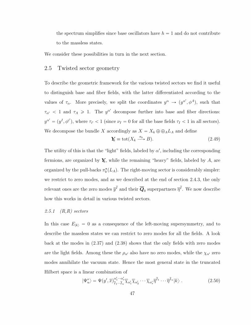
the spectrum simplifies since base oscillators have h “ 1 and do not contribute
to the massless states.
We consider these possibilities in turn in the next section.
2.5 Twisted sector geometry
To describe the geometric framework for the various twisted sectors we find it useful
to distinguish base and fiber fields, with the latter differentiated according to the
values of τα. More precisely, we split the coordinates yα Ñ pyα1
, φAq, such that
τα1 ă 1 and τA ě 1. The yα1
decompose further into base and fiber directions:
yα1
“ pyI , φi1
q, where τi1 ă 1 (since νI “ 0 for all the base fields τI ă 1 in all sectors).
We decompose the bundle X accordingly as X “ Xk ‘‘ALA and define
Yk ” totpXkπkÝÑ Bq. (2.49)
The utility of this is that the “light” fields, labeled by α1, including the corresponding
fermions, are organized by Yk, while the remaining “heavy” fields, labeled by A, are
organized by the pull-backs π˚kpLAq. The right-moving sector is considerably simpler:
we restrict to zero modes, and as we described at the end of section 2.4.3, the only
relevant ones are the zero modes yI and their Q0 superpartners ηI . We now describe
how this works in detail in various twisted sectors.
2.5.1 (R,R) sectors
In this case E|ky “ 0 as a consequence of the left-moving supersymmetry, and to
describe the massless states we can restrict to zero modes for all the fields. A look
back at the modes in (2.37) and (2.38) shows that the only fields with zero modes
are the light fields. Among these the ρα1 also have no zero modes, while the χα1 zero
modes annihilate the vacuum state. Hence the most general state in the truncated
Hilbert space is a linear combination of
|Ψsuy “ Ψpy1, xq
α11¨¨¨α1s
I1¨¨¨Iuχα11χα12 ¨ ¨ ¨χα1sη
I1 ¨ ¨ ¨ ηIu |ky . (2.50)
47
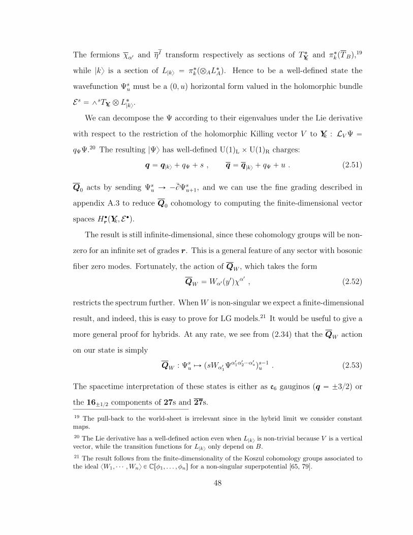
The fermions χα1 and ηI transform respectively as sections of T ˚Yk and π˚kpTBq,19
while |ky is a section of L|ky “ π˚kpbAL˚Aq. Hence to be a well-defined state the
wavefunction Ψsu must be a p0, uq horizontal form valued in the holomorphic bundle
Es “ ^sTYk b L˚|ky.
We can decompose the Ψ according to their eigenvalues under the Lie derivative
with respect to the restriction of the holomorphic Killing vector V to Yk : LV Ψ “
qΨΨ.20 The resulting |Ψy has well-defined Up1qL ˆ Up1qR charges:
q “ q|ky ` qΨ ` s , q “ q|ky ` qΨ ` u . (2.51)
Q0 acts by sending Ψsu Ñ ´BΨs
u`1, and we can use the fine grading described in
appendix A.3 to reduce Q0 cohomology to computing the finite-dimensional vector
spaces H‚rpYk, E‚q.
The result is still infinite-dimensional, since these cohomology groups will be non-
zero for an infinite set of grades r. This is a general feature of any sector with bosonic
fiber zero modes. Fortunately, the action of QW , which takes the form
QW “ Wα1py1qχα
1
, (2.52)
restricts the spectrum further. WhenW is non-singular we expect a finite-dimensional
result, and indeed, this is easy to prove for LG models.21 It would be useful to give a
more general proof for hybrids. At any rate, we see from (2.34) that the QW action
on our state is simply
QW : Ψsu ÞÑ psWα11
Ψα11α12¨¨¨α
1sqs´1u . (2.53)
The spacetime interpretation of these states is either as e6 gauginos (q “ ˘32) or
the 16˘12 components of 27s and 27s.
19 The pull-back to the world-sheet is irrelevant since in the hybrid limit we consider constantmaps.
20 The Lie derivative has a well-defined action even when L|ky is non-trivial because V is a verticalvector, while the transition functions for L|ky only depend on B.
21 The result follows from the finite-dimensionality of the Koszul cohomology groups associated tothe ideal xW1, ¨ ¨ ¨ ,Wny P Crφ1, . . . , φns for a non-singular superpotential [65, 79].
48
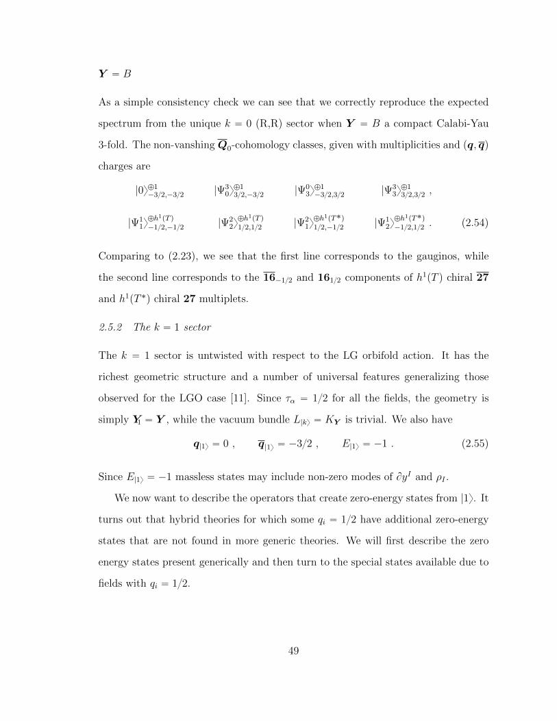
Y “ B
As a simple consistency check we can see that we correctly reproduce the expected
spectrum from the unique k “ 0 (R,R) sector when Y “ B a compact Calabi-Yau
3-fold. The non-vanshing Q0-cohomology classes, given with multiplicities and pq, qq
charges are
|0y‘1´32,´32 |Ψ3
0y‘132,´32 |Ψ0
3y‘1´32,32 |Ψ3
3y‘132,32 ,
|Ψ11y‘h1pT q´12,´12 |Ψ2
2y‘h1pT q12,12 |Ψ2
1y‘h1pT˚q12,´12 |Ψ1
2y‘h1pT˚q´12,12 . (2.54)
Comparing to (2.23), we see that the first line corresponds to the gauginos, while
the second line corresponds to the 16´12 and 1612 components of h1pT q chiral 27
and h1pT ˚q chiral 27 multiplets.
2.5.2 The k “ 1 sector
The k “ 1 sector is untwisted with respect to the LG orbifold action. It has the
richest geometric structure and a number of universal features generalizing those
observed for the LGO case [11]. Since τα “ 12 for all the fields, the geometry is
simply Y1 “ Y , while the vacuum bundle L|ky “ KY is trivial. We also have
q|1y “ 0 , q|1y “ ´32 , E|1y “ ´1 . (2.55)
Since E|1y “ ´1 massless states may include non-zero modes of ByI and ρI .
We now want to describe the operators that create zero-energy states from |1y. It
turns out that hybrid theories for which some qi “ 12 have additional zero-energy
states that are not found in more generic theories. We will first describe the zero
energy states present generically and then turn to the special states available due to
fields with qi “ 12.
49
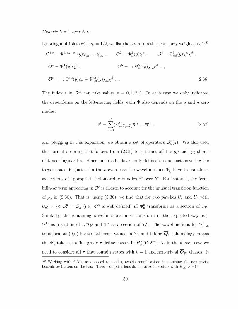
Generic k “ 1 operators
Ignoring multiplets with qi “ 12, we list the operators that can carry weight h ď 1:22
O1,s“ Ψ1sα1¨¨¨αspyqχα1
¨ ¨ ¨χαs , O2“ Ψ2
αpyqχα , O3
“ Ψ3αβpyqχ
αχβ ,
O4“ Ψ4
αpyqByα , O5
“ : Ψ5αβ pyqχαχ
β : ,
O6“ : Ψ6α
pyqρα `Ψ6α,βpyqχαχ
β : . (2.56)
The index s in O1s can take values s “ 0, 1, 2, 3. In each case we only indicated
the dependence on the left-moving fields; each Ψ also depends on the y and η zero
modes:
Ψt“
dÿ
u“0
pΨtuqI1¨¨¨Iu
ηI1 ¨ ¨ ¨ ηIu , (2.57)
and plugging in this expansion, we obtain a set of operators Otupzq. We also used
the normal ordering that follows from (2.31) to subtract off the yρ and χχ short-
distance singularities. Since our free fields are only defined on open sets covering the
target space Y , just as in the k even case the wavefunctions Ψt0 have to transform
as sections of appropriate holomorphic bundles E t over Y . For instance, the fermi
bilinear term appearing in O8 is chosen to account for the unusual transition function
of ρα in (2.36). That is, using (2.36), we find that for two patches Ua and Ub with
Uab ‰ H O6b “ O6
a (i.e. O6 is well-defined) iff Ψ60 transforms as a section of TY .
Similarly, the remaining wavefunctions must transform in the expected way, e.g.
Ψ1s0 as a section of ^sTY and Ψ2
0 as a section of T ˚Y . The wavefunctions for Ψtuą0
transform as (0,u) horizontal forms valued in E t, and taking Q0 cohomology means
the Ψtu taken at a fine grade r define classes in H‚
rpY , E‚q. As in the k even case we
need to consider all r that contain states with h “ 1 and non-trivial QW classes. It
22 Working with fields, as opposed to modes, avoids complications in patching the non-trivialbosonic oscillators on the base. These complications do not arise in sectors with E|ky ą ´1.
50
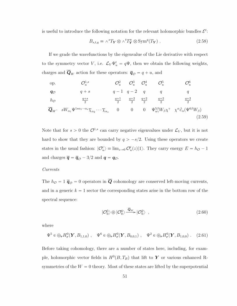
is useful to introduce the following notation for the relevant holomorphic bundles E t:
Bs,t,q ” ^sTY b^
tT ˚Y b SymqpTY q . (2.58)
If we grade the wavefunctions by the eigenvalue of the Lie derivative with respect
to the symmetry vector V , i.e. LV Ψtu “ qΨ, then we obtain the following weights,
charges and QW action for these operators: qO “ q ` u, and
op. O1,su O2
u O3u O4
u O5u O6
u
qO q ` s q ´ 1 q ´ 2 q q q
hOq`s
2q`1
2q`2
2q`2
2q`2
2q`2
2
QW ¨ sWα1Ψ1sα1¨¨¨αsχα2¨ ¨ ¨χαs 0 0 0 Ψ5β
uγWβχγ χαBαpΨ
6βWβq
(2.59)
Note that for s ą 0 the O1,s can carry negative eigenvalues under LV , but it is not
hard to show that they are bounded by q ą ´s2. Using these operators we create
states in the usual fashion: |Otuy ” limzÑ0Otupzq|1y. They carry energy E “ hO ´ 1
and charges q “ qO ´ 32 and q “ qO.
Currents
The hO “ 1 qO “ 0 operators in Q cohomology are conserved left-moving currents,
and in a generic k “ 1 sector the corresponding states arise in the bottom row of the
spectral sequence:
|O50y ‘ |O6
0yQW // |O2
0y , (2.60)
where
Ψ5P ‘rH
0rpY , B1,1,0q , Ψ6
P ‘rH0rpY , B0,0,1q , Ψ2
P ‘rH0rpY , B1,0,0q . (2.61)
Before taking cohomology, there are a number of states here, including, for exam-
ple, holomorphic vector fields in H0pB, TBq that lift to Y or various enhanced R-
symmetries of the W “ 0 theory. Most of these states are lifted by the superpotential
51
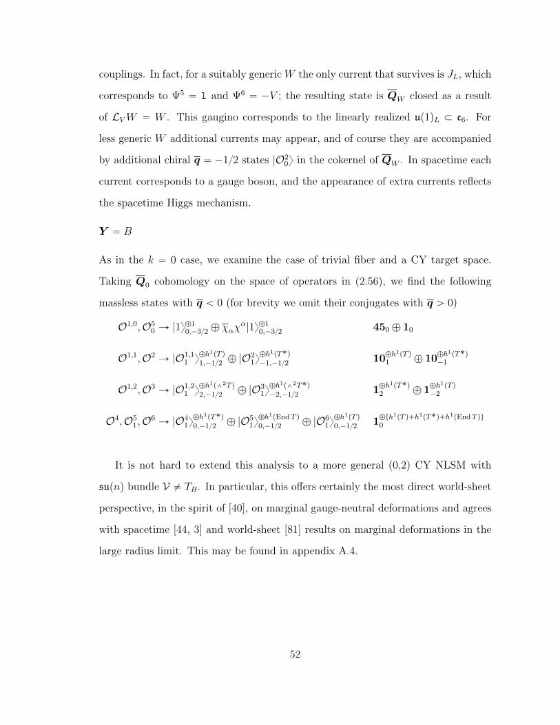
couplings. In fact, for a suitably generic W the only current that survives is JL, which
corresponds to Ψ5 “ 1 and Ψ6 “ ´V ; the resulting state is QW closed as a result
of LVW “ W . This gaugino corresponds to the linearly realized up1qL Ă e6. For
less generic W additional currents may appear, and of course they are accompanied
by additional chiral q “ ´12 states |O20y in the cokernel of QW . In spacetime each
current corresponds to a gauge boson, and the appearance of extra currents reflects
the spacetime Higgs mechanism.
Y “ B
As in the k “ 0 case, we examine the case of trivial fiber and a CY target space.
Taking Q0 cohomology on the space of operators in (2.56), we find the following
massless states with q ă 0 (for brevity we omit their conjugates with q ą 0)
O1,0,O50 Ñ |1y‘1
0,´32 ‘ χαχα|1y‘1
0,´32 450 ‘ 10
O1,1,O2Ñ |O1,1
1 y‘h1pT q1,´12 ‘ |O
21y‘h1pT˚q´1,´12 10
‘h1pT q1 ‘ 10
‘h1pT˚q´1
O1,2,O3Ñ |O1,2
1 y‘h1p^2T q2,´12 ‘ |O3
1y‘h1p^2T˚q´2,´12 1
‘h1pT˚q2 ‘ 1
‘h1pT q´2
O4,O51,O6
Ñ |O41y‘h1pT˚q0,´12 ‘ |O5
1y‘h1pEndT q0,´12 ‘ |O6
1y‘h1pT q0,´12 1
‘th1pT q`h1pT˚q`h1pEndT qu0
It is not hard to extend this analysis to a more general (0,2) CY NLSM with
supnq bundle V ‰ TB. In particular, this offers certainly the most direct world-sheet
perspective, in the spirit of [40], on marginal gauge-neutral deformations and agrees
with spacetime [44, 3] and world-sheet [81] results on marginal deformations in the
large radius limit. This may be found in appendix A.4.
52
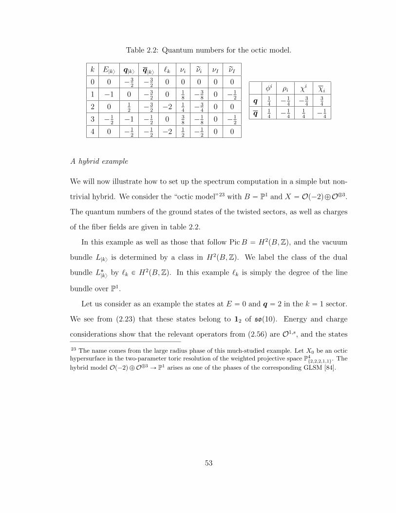
Table 2.2: Quantum numbers for the octic model.
k E|ky q|ky q|ky `k νi rνi νI rνI
0 0 ´32
´32
0 0 0 0 0
1 ´1 0 ´32
0 18
´38
0 ´12
2 0 12
´32
´2 14
´34
0 0
3 ´12
´1 ´12
0 38
´18
0 ´12
4 0 ´12
´12
´2 12
´12
0 0
φi ρi χi χi
q 14
´14´3
434
q 14
´14
14
´14
A hybrid example
We will now illustrate how to set up the spectrum computation in a simple but non-
trivial hybrid. We consider the “octic model”23 with B “ P1 and X “ Op´2q‘O‘3.
The quantum numbers of the ground states of the twisted sectors, as well as charges
of the fiber fields are given in table 2.2.
In this example as well as those that follow PicB “ H2pB,Zq, and the vacuum
bundle L|ky is determined by a class in H2pB,Zq. We label the class of the dual
bundle L˚|ky by `k P H
2pB,Zq. In this example `k is simply the degree of the line
bundle over P1.
Let us consider as an example the states at E “ 0 and q “ 2 in the k “ 1 sector.
We see from (2.23) that these states belong to 12 of sop10q. Energy and charge
considerations show that the relevant operators from (2.56) are O1,s, and the states
23 The name comes from the large radius phase of this much-studied example. Let X0 be an octichypersurface in the two-parameter toric resolution of the weighted projective space P4
t2,2,2,1,1u. The
hybrid model Op´2q ‘O‘3 Ñ P1 arises as one of the phases of the corresponding GLSM [84].
53
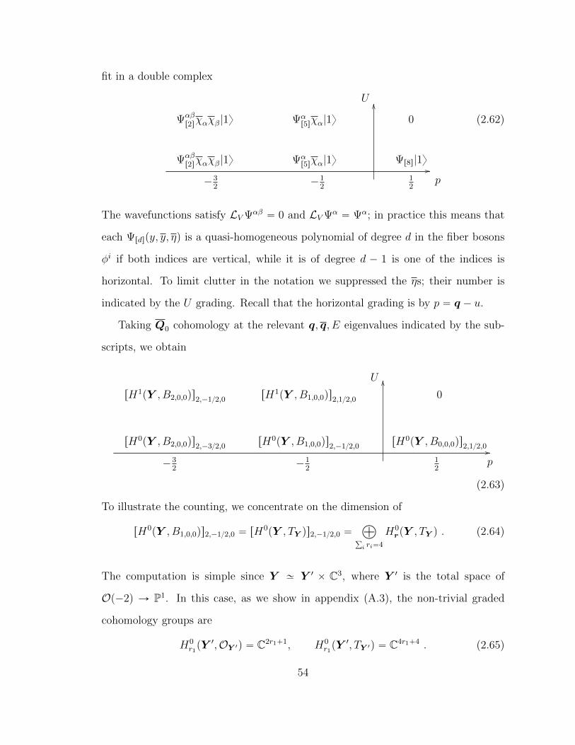
fit in a double complex
Ψαβr2sχαχβ|1y Ψα
r5sχα|1y 0
Ψαβr2sχαχβ|1y Ψα
r5sχα|1y Ψr8s|1y//
OO
´32
´12
12
p
U
(2.62)
The wavefunctions satisfy LV Ψαβ “ 0 and LV Ψα “ Ψα; in practice this means that
each Ψrdspy, y, ηq is a quasi-homogeneous polynomial of degree d in the fiber bosons
φi if both indices are vertical, while it is of degree d ´ 1 is one of the indices is
horizontal. To limit clutter in the notation we suppressed the ηs; their number is
indicated by the U grading. Recall that the horizontal grading is by p “ q ´ u.
Taking Q0 cohomology at the relevant q, q, E eigenvalues indicated by the sub-
scripts, we obtain
rH1pY , B2,0,0qs2,´12,0 rH1pY , B1,0,0qs2,12,0 0
rH0pY , B2,0,0qs2,´32,0 rH0pY , B1,0,0qs2,´12,0 rH0pY , B0,0,0qs2,12,0 //
OO
´32
´12
12
p
U
(2.63)
To illustrate the counting, we concentrate on the dimension of
rH0pY , B1,0,0qs2,´12,0 “ rH
0pY , TY qs2,´12,0 “
à
ř
i ri“4
H0rpY , TY q . (2.64)
The computation is simple since Y » Y 1 ˆ C3, where Y 1 is the total space of
Op´2q Ñ P1. In this case, as we show in appendix (A.3), the non-trivial graded
cohomology groups are
H0r1pY 1,OY 1q “ C2r1`1, H0
r1pY 1, TY 1q “ C4r1`4 . (2.65)
54
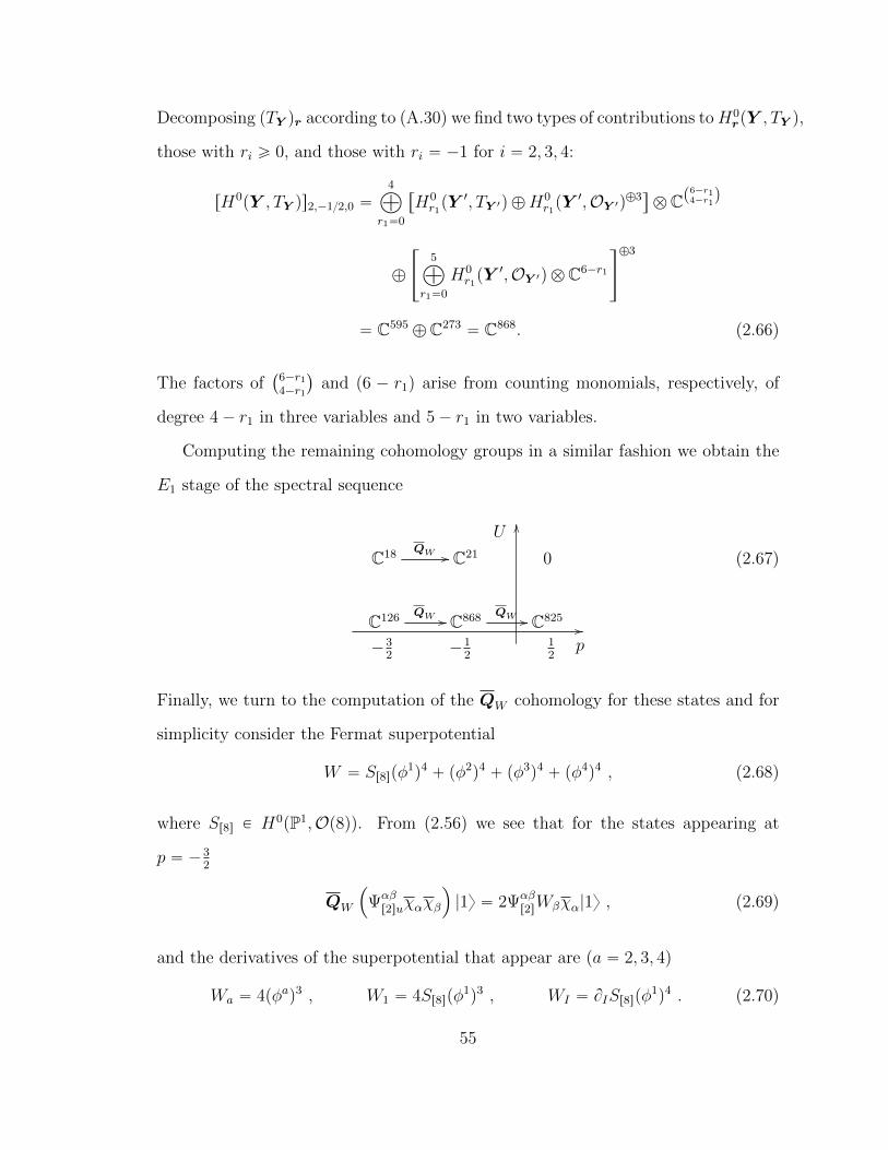
Decomposing pTY qr according to (A.30) we find two types of contributions toH0rpY , TY q,
those with ri ě 0, and those with ri “ ´1 for i “ 2, 3, 4:
rH0pY , TY qs2,´12,0 “
4à
r1“0
“
H0r1pY 1, TY 1q ‘H
0r1pY 1,OY 1q
‘3‰
b Cp6´r14´r1q
‘
«
5à
r1“0
H0r1pY 1,OY 1q b C6´r1
ff‘3
“ C595‘ C273
“ C868. (2.66)
The factors of`
6´r14´r1
˘
and p6 ´ r1q arise from counting monomials, respectively, of
degree 4´ r1 in three variables and 5´ r1 in two variables.
Computing the remaining cohomology groups in a similar fashion we obtain the
E1 stage of the spectral sequence
C18 QW // C21 0
C126 QW // C868 QW // C825//
OO
´32
´12
12
p
U
(2.67)
Finally, we turn to the computation of the QW cohomology for these states and for
simplicity consider the Fermat superpotential
W “ Sr8spφ1q4` pφ2
q4` pφ3
q4` pφ4
q4 , (2.68)
where Sr8s P H0pP1,Op8qq. From (2.56) we see that for the states appearing at
p “ ´32
QW
´
Ψαβr2suχαχβ
¯
|1y “ 2Ψαβr2sWβχα|1y , (2.69)
and the derivatives of the superpotential that appear are (a “ 2, 3, 4)
Wa “ 4pφaq3 , W1 “ 4Sr8spφ1q3 , WI “ BISr8spφ
1q4 . (2.70)
55
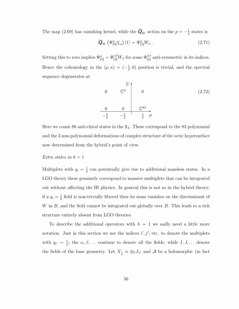
The map (2.69) has vanishing kernel, while the QW action on the p “ ´12
states is
QW
`
Ψαr5sχα
˘
|1y “ Ψαr5sWα . (2.71)
Setting this to zero implies Ψαr5s “ Φαβ
r2sWβ for some Φαβr2s anti-symmetric in its indices.
Hence the cohomology in the pp, uq “ p´12, 0q position is trivial, and the spectral
sequence degenerates at
0 C3 0
0 0 C83//
OO
´32
´12
12
p
U
(2.72)
Here we count 86 anti-chiral states in the 12. These correspond to the 83 polynomial
and the 3 non-polynomial deformations of complex structure of the octic hypersurface
now determined from the hybrid’s point of view.
Extra states in k “ 1
Multiplets with qi “12
can potentially give rise to additional massless states. In a
LGO theory these genuinely correspond to massive multiplets that can be integrated
out without affecting the IR physics. In general this is not so in the hybrid theory:
if a qi “12
field is non-trivially fibered then its mass vanishes on the discriminant of
W in B, and the field cannot be integrated out globally over B. This leads to a rich
structure entirely absent from LGO theories.
To describe the additional operators with h “ 1 we sadly need a little more
notation. Just in this section we use the indices i1, j1, etc. to denote the multiplets
with qi1 “12; the α, β, . . . continue to denote all the fields, while I, J, . . . denote
the fields of the base geometry. Let X 12” ‘i1Li1 and A be a holomorphic (in fact
56
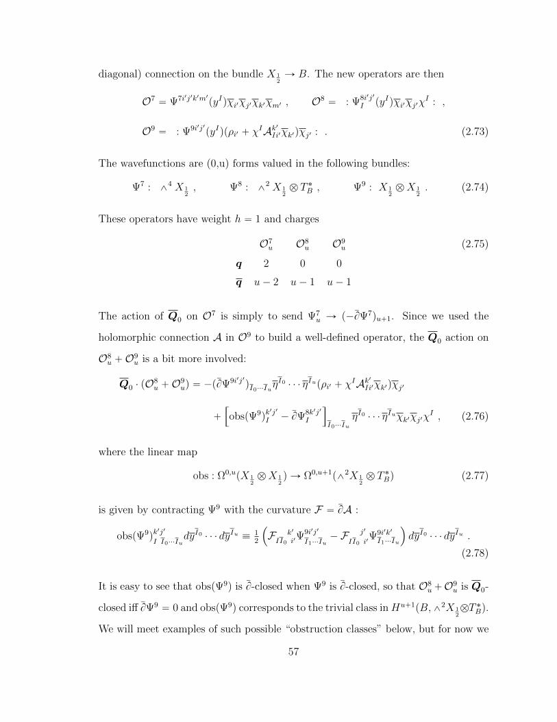
diagonal) connection on the bundle X 12Ñ B. The new operators are then
O7“ Ψ7i1j1k1m1
pyIqχi1χj1χk1χm1 , O8“ : Ψ8i1j1
I pyIqχi1χj1χI : ,
O9“ : Ψ9i1j1
pyIqpρi1 ` χIAk1Ii1χk1qχj1 : . (2.73)
The wavefunctions are (0,u) forms valued in the following bundles:
Ψ7 : ^4 X 1
2, Ψ8 : ^
2 X 12b T ˚B , Ψ9 : X 1
2bX 1
2. (2.74)
These operators have weight h “ 1 and charges
O7u O8
u O9u
q 2 0 0
q u´ 2 u´ 1 u´ 1
(2.75)
The action of Q0 on O7 is simply to send Ψ7u Ñ p´BΨ7qu`1. Since we used the
holomorphic connection A in O9 to build a well-defined operator, the Q0 action on
O8u `O9
u is a bit more involved:
Q0 ¨ pO8u `O9
uq “ ´pBΨ9i1j1qI0¨¨¨Iu
ηI0 ¨ ¨ ¨ ηIupρi1 ` χIAk1Ii1χk1qχj1
`
”
obspΨ9qk1j1
I ´ BΨ8k1j1
I
ı
I0¨¨¨IuηI0 ¨ ¨ ¨ ηIuχk1χj1χ
I , (2.76)
where the linear map
obs : Ω0,upX 1
2bX 1
2q Ñ Ω0,u`1
p^2X 1
2b T ˚Bq (2.77)
is given by contracting Ψ9 with the curvature F “ BA :
obspΨ9qk1j1
I I0¨¨¨IudyI0 ¨ ¨ ¨ dyIu ” 1
2
´
F k1
II0 i1Ψ9i1j1
I1¨¨¨Iu´ F j1
II0 i1Ψ9i1k1
I1¨¨¨Iu
¯
dyI0 ¨ ¨ ¨ dyIu .
(2.78)
It is easy to see that obspΨ9q is B-closed when Ψ9 is B-closed, so that O8u`O9
u is Q0-
closed iff BΨ9 “ 0 and obspΨ9q corresponds to the trivial class inHu`1pB,^2X 12bT ˚Bq.
We will meet examples of such possible “obstruction classes” below, but for now we
57
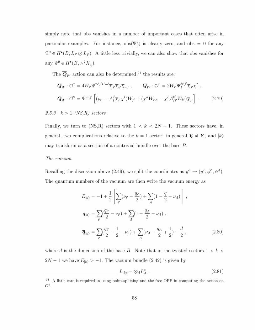
simply note that obs vanishes in a number of important cases that often arise in
particular examples. For instance, obspΨ9dq is clearly zero, and obs “ 0 for any
Ψ9 P H‚pB,Lj1 b Lj1q. A little less trivially, we can also show that obs vanishes for
any Ψ9 P H‚pB,^2X 12q.
The QW action can also be determined;24 the results are:
QW ¨O7“ 4Wi1Ψ
7i1j1k1m1χj1χk1χm1 , QW ¨O8“ 2Wi1Ψ
8i1j1
I χj1χI ,
QW ¨O9“ Ψ9i1j1
”
pρi1 ´Ai1
I χi1χIqWj1 ` pχ
αWi1α ´ χIAk1Ii1Wk1qχj1
ı
. (2.79)
2.5.3 k ą 1 (NS,R) sectors
Finally, we turn to (NS,R) sectors with 1 ă k ă 2N ´ 1. These sectors have, in
general, two complications relative to the k “ 1 sector: in general Yk ‰ Y , and |ky
may transform as a section of a nontrivial bundle over the base B.
The vacuum
Recalling the discussion above (2.49), we split the coordinates as yα Ñ pyI , φi1
, φAq.
The quantum numbers of the vacuum are then write the vacuum energy as
E|ky “ ´1`1
2
«
ÿ
i1
pνi1 ´qi1
2q `
ÿ
A
p1´q
2´ νAq
ff
,
q|ky “ÿ
i1
pqi1
2´ νi1q `
ÿ
A
p1´qA2´ νAq ,
q|ky “ÿ
i1
pqi1
2´
1
2´ νi1q `
ÿ
A
pνA ´qA2`
1
2q ´
d
2, (2.80)
where d is the dimension of the base B. Note that in the twisted sectors 1 ă k ă
2N ´ 1 we have E|ky ą ´1. The vacuum bundle (2.42) is given by
L|ky “ bAL˚A . (2.81)
24 A little care is required in using point-splitting and the free OPE in computing the action onO9.
58
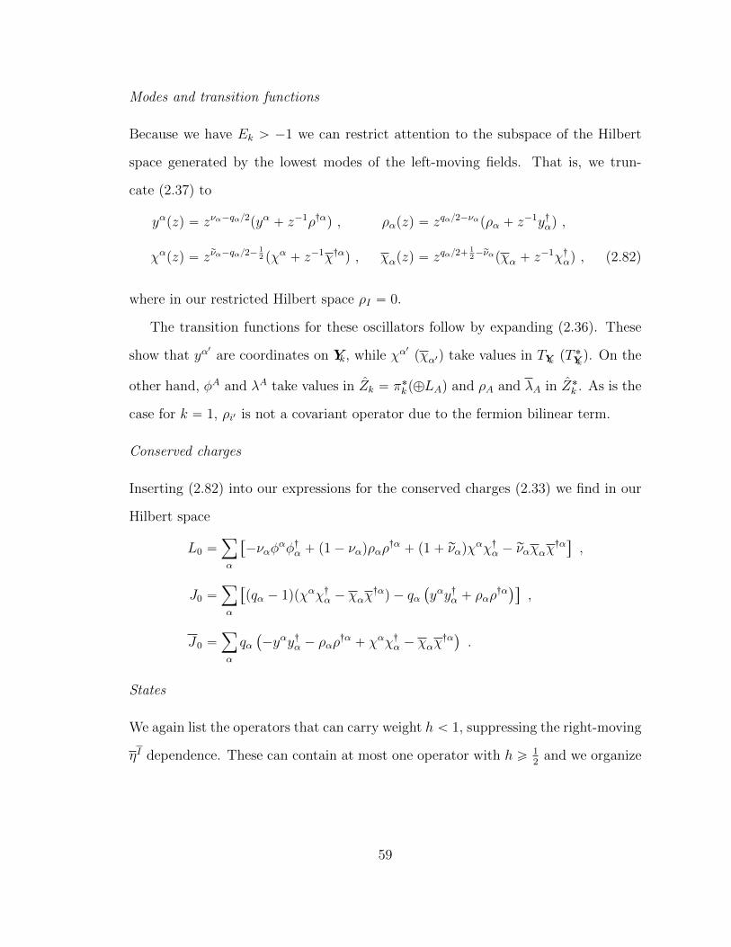
Modes and transition functions
Because we have Ek ą ´1 we can restrict attention to the subspace of the Hilbert
space generated by the lowest modes of the left-moving fields. That is, we trun-
cate (2.37) to
yαpzq “ zνα´qα2pyα ` z´1ρ:αq , ραpzq “ zqα2´ναpρα ` z´1y:αq ,
χαpzq “ zrνα´qα2´12 pχα ` z´1χ:αq , χαpzq “ zqα2`
12´rναpχα ` z
´1χ:αq , (2.82)
where in our restricted Hilbert space ρI “ 0.
The transition functions for these oscillators follow by expanding (2.36). These
show that yα1
are coordinates on Yk, while χα1
(χα1) take values in TYk (T ˚Yk). On the
other hand, φA and λA take values in Zk “ π˚kp‘LAq and ρA and λA in Z˚k . As is the
case for k “ 1, ρi1 is not a covariant operator due to the fermion bilinear term.
Conserved charges
Inserting (2.82) into our expressions for the conserved charges (2.33) we find in our
Hilbert space
L0 “ÿ
α
“
´ναφαφ:α ` p1´ ναqραρ
:α` p1` rναqχ
αχ:α ´ rναχαχ:α‰
,
J0 “ÿ
α
“
pqα ´ 1qpχαχ:α ´ χαχ:αq ´ qα
`
yαy:α ` ραρ:α˘‰
,
J0 “ÿ
α
qα`
´yαy:α ´ ραρ:α` χαχ:α ´ χαχ
:α˘
.
States
We again list the operators that can carry weight h ă 1, suppressing the right-moving
ηI dependence. These can contain at most one operator with h ě 12
and we organize
59
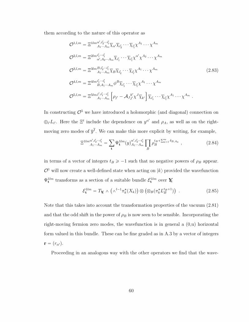
them according to the nature of this operator as
O1,l,m“ Ξ1lmα
1,i12¨¨¨i1l
A1¨¨¨Amχα1χi12 ¨ ¨ ¨χi1lχ
A1 ¨ ¨ ¨χAm
O2,l,m“ Ξ2lmi
11¨¨¨i
1l
α1,A2¨¨¨Amχi11 ¨ ¨ ¨χi1lχ
α1χA2 ¨ ¨ ¨χAm
O3,l,m“ Ξ3lmB,i
12¨¨¨i
1l
A1¨¨¨AmχBχi12 ¨ ¨ ¨χi1lχ
A1 ¨ ¨ ¨χAm (2.83)
O4,l,m“ Ξ4lmi
11¨¨¨i
1l
B,A1¨¨¨AmφBχi11 ¨ ¨ ¨χi1lχ
A1 ¨ ¨ ¨χAm
O5,l,m“ Ξ5lmj
1,i11¨¨¨i1l
A1¨¨¨Am
”
ρj1 ´AJk1
j1χJχk1
ı
χi11 ¨ ¨ ¨χi1lχA1 ¨ ¨ ¨χAm .
In constructing O5 we have introduced a holomorphic (and diagonal) connection on
‘i1Li1 . Here the Ξt include the dependence on yα1
and ρA, as well as on the right-
moving zero modes of yI . We can make this more explicit by writing, for example,
Ξ1lmα1,i12¨¨¨i
1l
A1¨¨¨Am“ÿ
t
Ψ1lmt pyq
α1,i12¨¨¨i1l
A1¨¨¨Am
ź
B
ρtB`
řma“1 δB,Aa
B , (2.84)
in terms of a vector of integers tB ě ´1 such that no negative powers of ρB appear.
O1 will now create a well-defined state when acting on |ky provided the wavefunction
Ψ1lmt transforms as a section of a suitable bundle E1lm
t over Yk
E1lmt “ TYk ^
`
^l´1π˚kpXkq
˘
b`
bBpπ˚kL
tB`1B q
˘
. (2.85)
Note that this takes into account the transformation properties of the vacuum (2.81)
and that the odd shift in the power of ρB is now seen to be sensible. Incorporating the
right-moving fermion zero modes, the wavefunction is in general a (0,u) horizontal
form valued in this bundle. These can be fine graded as in A.3 by a vector of integers
r “ prα1q.
Proceeding in an analogous way with the other operators we find that the wave-
60
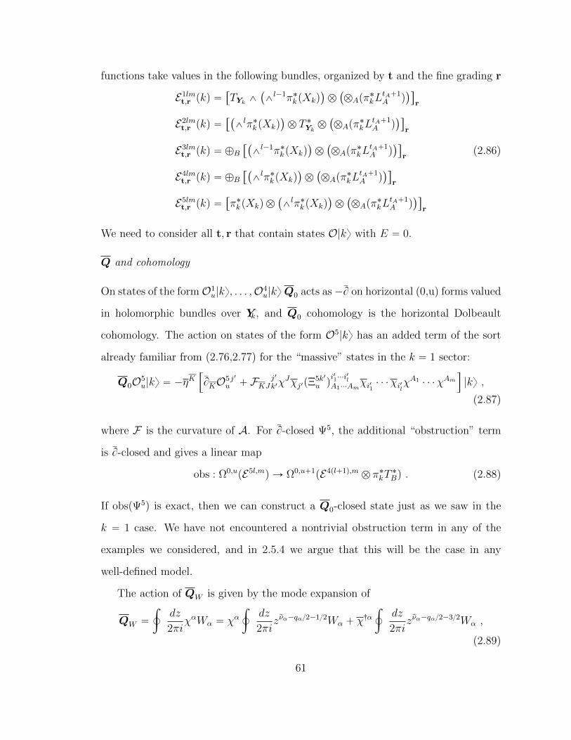
functions take values in the following bundles, organized by t and the fine grading r
E1lmt,r pkq “
“
TYk ^`
^l´1π˚kpXkq
˘
b`
bApπ˚kL
tA`1A q
˘‰
r
E2lmt,r pkq “
“`
^lπ˚kpXkq
˘
b T ˚Yk b`
bApπ˚kL
tA`1A q
˘‰
r
E3lmt,r pkq “ ‘B
“`
^l´1π˚kpXkq
˘
b`
bApπ˚kL
tA`1A q
˘‰
r(2.86)
E4lmt,r pkq “ ‘B
“`
^lπ˚kpXkq
˘
b`
bApπ˚kL
tA`1A q
˘‰
r
E5lmt,r pkq “
“
π˚kpXkq b`
^lπ˚kpXkq
˘
b`
bApπ˚kL
tA`1A q
˘‰
r
We need to consider all t, r that contain states O|ky with E “ 0.
Q and cohomology
On states of the formO1u|ky, . . . ,O4
u|kyQ0 acts as ´B on horizontal (0,u) forms valued
in holomorphic bundles over Yk, and Q0 cohomology is the horizontal Dolbeault
cohomology. The action on states of the form O5|ky has an added term of the sort
already familiar from (2.76,2.77) for the “massive” states in the k “ 1 sector:
Q0O5u|ky “ ´η
K”
BKO5uj1` FKJ
j1
k1χJχj1pΞ
5k1
u qi11¨¨¨i
1l
A1¨¨¨Amχi11 ¨ ¨ ¨χi1lχ
A1 ¨ ¨ ¨χAmı
|ky ,
(2.87)
where F is the curvature of A. For B-closed Ψ5, the additional “obstruction” term
is B-closed and gives a linear map
obs : Ω0,upE5l,m
q Ñ Ω0,u`1pE4pl`1q,m
b π˚kT˚Bq . (2.88)
If obspΨ5q is exact, then we can construct a Q0-closed state just as we saw in the
k “ 1 case. We have not encountered a nontrivial obstruction term in any of the
examples we considered, and in 2.5.4 we argue that this will be the case in any
well-defined model.
The action of QW is given by the mode expansion of
QW “
¿
dz
2πiχαWα “ χα
¿
dz
2πizrνα´qα2´12Wα ` χ
:α
¿
dz
2πizrνα´qα2´32Wα ,
(2.89)
61
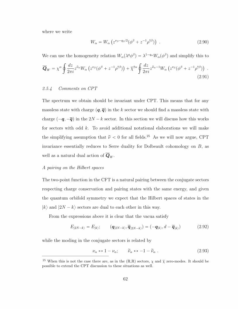
where we write
Wα “ Wα
`
zνβ´qβ2pφβ ` z´1ρ:βq˘
. (2.90)
We can use the homogeneity relation Wαpλqφβq “ λ1´qαWαpφ
βq and simplify this to
QW “ χα¿
dz
2πizrναWα
`
zνβpφβ ` z´1ρ:βq˘
` χ:α¿
dz
2πizrνα´1Wα
`
zνβpφβ ` z´1ρ:βq˘
.
(2.91)
2.5.4 Comments on CPT
The spectrum we obtain should be invariant under CPT. This means that for any
massless state with charge pq, qq in the k sector we should find a massless state with
charge p´q,´qq in the 2N ´ k sector. In this section we will discuss how this works
for sectors with odd k. To avoid additional notational elaborations we will make
the simplifying assumption that rν ă 0 for all fields.25 As we will now argue, CPT
invariance essentially reduces to Serre duality for Dolbeault cohomology on B, as
well as a natural dual action of QW .
A pairing on the Hilbert spaces
The two-point function in the CFT is a natural pairing between the conjugate sectors
respecting charge conservation and pairing states with the same energy, and given
the quantum orbifold symmetry we expect that the Hilbert spaces of states in the
|ky and |2N ´ ky sectors are dual to each other in this way.
From the expressions above it is clear that the vacua satisfy
E|2N´ky “ E|ky; pq|2N´ky, q|2N´kyq “ p´q|ky, d´ q|kyq (2.92)
while the moding in the conjugate sectors is related by
να Ø 1´ να; rνα Ø ´1´ rνα . (2.93)
25 When this is not the case there are, as in the (R,R) sectors, χ and χ zero-modes. It should bepossible to extend the CPT discussion to these situations as well.
62
This implies that the fields φi1
for which τ “ 12 in the k sector have τ “ 32 in the
conjugate 2N ´ k sector, and vice versa, so that we have
Yk “ totp‘i1Li1ÑBq L|ky “ bAL˚A
Y2N´k “ totp‘LAÑBq L|2N´ky “ bi1L˚i1 . (2.94)
In particular L|ky b L|2N´ky “ K˚B. For any state with weight h and charge pq, qq in
the k sector, we can find a state with the same weight and charge p´q, d´ qq in the
2N ´ k sector by exchanging the oscillator excitations according to
yα Ø ρα χα Ø χα . (2.95)
This is enough to show that at the level of left-moving oscillators the two-point
function leads to a pairing between the state spaces defined above, which respects q
and violates q by d. If we denote Htlmt,r pkq “ ΓpE tlmt,r pkqq, then the pairing takes the
form
H1‘2‘3lmt,rpkq ˆH1‘2‘3ml
r,tp2N ´ kq Ñ C
H4lmt,r pkq ˆH5ml
r,t p2N ´ kq Ñ C , (2.96)
Q0 and Serre duality
The pairing descends to Q0 cohomology, and in a reasonable physical theory this
must be nondegenerate. This will be the case if
H‚
Q0
`
Hlmk pt, rq
˘
“
”
Hd´‚
Q0
`
Hml2N´kpr, tq
˘
ı˚
. (2.97)
For the first line in (2.96), in which Q0 acts as ´B, this is in fact equivalent to Serre
duality. For simplicity let’s see first how this works in H111r,t . The fine grading on
H‚pTYkq can be obtained from the long exact sequence (LES) following from the
short exact sequence (SES) (A.29)
0 // ‘ipπ˚kLiqr`xi
// pTYkqr// pπ˚kTBqr
// 0 , (2.98)
63
which we here encounter twisted by a vector bundle (so still exact) as
0 // ‘ipπ˚kLiqr`xi b
pVt // pTYkqr bpVt // pπ˚kTBqr b
pVt // 0 , (2.99)
where
pVt “ π˚k“
‘B`
bApLtA`1A q
˘‰
. (2.100)
The bundles on either end of the SES are pulled back from B, and we can use (A.20)
to compute their cohomology. Thus
H‚r
´
Yk,‘ipπ˚kLiqr`xi b
pVt
¯
“ H‚`
B,‘i,B`
bApLtA`1A q b
`
bjpL˚j qrj˘˘˘
, (2.101)
while
H‚r
´
Yk, pπ˚k TBqr b
pVt
¯
“ H‚`
B, TB b`
‘B`
bApLtA`1A q b
`
bjpL˚j qrj˘˘˘˘
. (2.102)
Recalling that KB “ bαLα, these are Serre dual, respectively, to
Hd´‚`
B,‘i,B`
bApL˚Aq
tA b`
bjpLjqrj`1
˘˘˘
“ Hd´‚´
Y2N´k,‘i,B
´
π˚2N´kpL˚Aqt´yA b
´
bjpLrj`1j q
¯¯¯
(2.103)
and
Hd´‚´
B, T ˚B b´
‘B
´
bApL˚Aq
tA b
´
bjpLrj`1j q
¯¯¯¯
“ Hd´‚`
Y2N´k,`
π˚2N´k T˚B
˘
tb`
‘jpπ˚2N´kpLjq
rj`1q˘˘
. (2.104)
Inserting this result into the dual LES we find
H‚ppTYkqr b
pVtq “”
Hd´‚ppTY2N´kqt b
pVrqı˚
(2.105)
with a suitable natural definition for pVr.
Higher powers of the tangent/cotangent bundles are fine graded by recursively
using the same SES and the dual, so recursively applying this argument we find
that Serre duality implies CPT in the sense above whenever we can use Q0 “ ´B.
This argument will fail if nontrivial obstruction classes arise in (2.87), because no
such obstruction can arise for the dual states in H4. We conclude that in reasonable
physical theories there will be no nontrivial obstructions in the twisted sectors.
64
QW and CPT
Given that the cohomology of Q0 produces a spectrum consistent with CPT, we can
also show that the action of QW is consistent with this. Consider a monomial in Wα
that contributes to QW in the k sector a term
χαź
β
“
pφβqmβpρ:βqnβ‰
. (2.106)
This means thatÿ
β
rνβ,kpmβ ` nβq ´ nβs “ ´rνα,k ´ 1 . (2.107)
Using (2.93) we see that this impliesÿ
β
rνβ,2N´kpmβ ` nβq ´mβs “ÿ
β
r´νβ,kpmβ ` nβq ` nβs “ rνα,k ` 1 “ ´rνα,2N´k ,
(2.108)
which means that the same monomial contributes a term
χ:αź
β
“
pφβqnβpρ:βqmβ‰
(2.109)
to QW in the 2N ´ k sector. This acts in precisely the appropriately dual way on
the states as mapped above, showing that CPT is maintained as a symmetry after
taking QW cohomology.
2.6 Examples
In this section we will apply the techniques developed in the previous sections to a
number of hybrid examples. In each case we will focus on characterizing first order
deformations that preserve (0,2) superconformal invariance and the e8‘ e6 spacetime
gauge symmetry.
The infinitesimal deformations which preserve (2,2) symmetry parametrize the
tangent space of the (2,2) moduli space. They are not obstructed and in a large
65
radius limit are identified with complex structure and complexified Kahler moduli of
the CY. There is a well-known correspondence between the (2,2) moduli and the e6-
charged matter, and we will borrow the large radius notation by denoting the number
of chiral 27’s and 27’s in the hybrid computation by h1,1 and h2,1 respectively.
More interesting are the deformations which only preserve (0,2) superconformal
invariance. The computation of the number of massless gauge singlets associated to
these deformations, which we indicate asM, is the main goal of this section. These
singlets arise in (NS,R), i.e. the odd k sectors. In the following we will compute M
in three examples that illustrate a number of technical and conceptual points.
1. For the first example we choose the simplest possible base, i.e. B “ P1. This is
a good warm-up for more difficult cases and is of interest in its own right since
the model can be found as a phase of a GLSM without a large radius limit in
its Kahler moduli space. In fact, it can be shown [6] that h1,1 “ 1, and the
only other phase is a LGO.
2. In the second example we describe a model in the broader orbi-bundle set-up
with B “ P3. It will be clear that most of our discussion above was restricted
to the case in which X is a sum of line bundles solely for ease of exposition.
This example also give us a chance to compute a higher order differential (it
will turn out to be zero).
3. In the last example we consider the case in which one of the line bundles
defining X is positive, and B “ F0 is not a projective space.
While our construction does not depend on a GLSM embedding, all of these
models do arise as phases of a GLSM. That gives us the possibility to compare the
hybrid spectrum with the spectrum known in other phases. What we discover is that
while in the hybrid limit extra singlets appear at a particular complex structure or
66
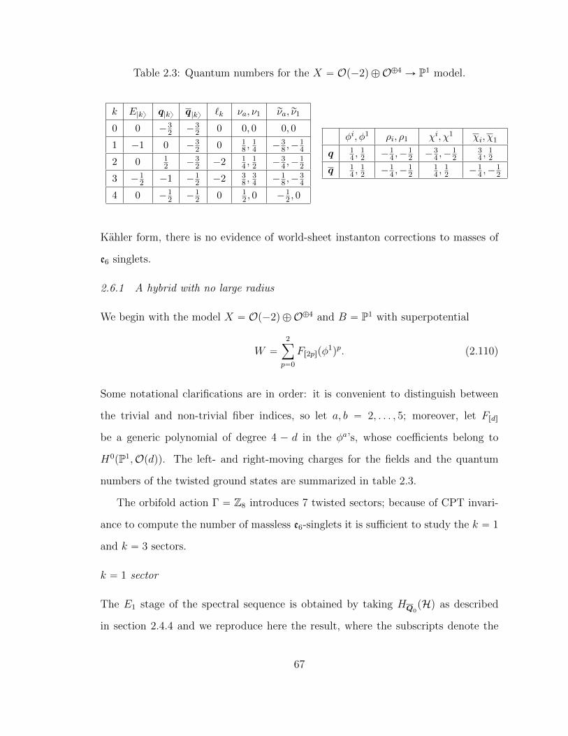
Table 2.3: Quantum numbers for the X “ Op´2q ‘O‘4 Ñ P1 model.
k E|ky q|ky q|ky `k νa, ν1 rνa, rν1
0 0 ´32 ´3
2 0 0, 0 0, 0
1 ´1 0 ´32 0 1
8 ,14 ´3
8 ,´14
2 0 12 ´3
2 ´2 14 ,
12 ´3
4 ,´12
3 ´12 ´1 ´1
2 ´2 38 ,
34 ´1
8 ,´34
4 0 ´12 ´1
2 0 12 , 0 ´1
2 , 0
φi, φ1 ρi, ρ1 χi, χ1 χi, χ1
q 14 ,
12 ´1
4 ,´12 ´3
4 ,´12
34 ,
12
q 14 ,
12 ´1
4 ,´12
14 ,
12 ´1
4 ,´12
Kahler form, there is no evidence of world-sheet instanton corrections to masses of
e6 singlets.
2.6.1 A hybrid with no large radius
We begin with the model X “ Op´2q ‘O‘4 and B “ P1 with superpotential
W “
2ÿ
p“0
Fr2pspφ1qp. (2.110)
Some notational clarifications are in order: it is convenient to distinguish between
the trivial and non-trivial fiber indices, so let a, b “ 2, . . . , 5; moreover, let Frds
be a generic polynomial of degree 4 ´ d in the φa’s, whose coefficients belong to
H0pP1,Opdqq. The left- and right-moving charges for the fields and the quantum
numbers of the twisted ground states are summarized in table 2.3.
The orbifold action Γ “ Z8 introduces 7 twisted sectors; because of CPT invari-
ance to compute the number of massless e6-singlets it is sufficient to study the k “ 1
and k “ 3 sectors.
k “ 1 sector
The E1 stage of the spectral sequence is obtained by taking HQ0pHq as described
in section 2.4.4 and we reproduce here the result, where the subscripts denote the
67
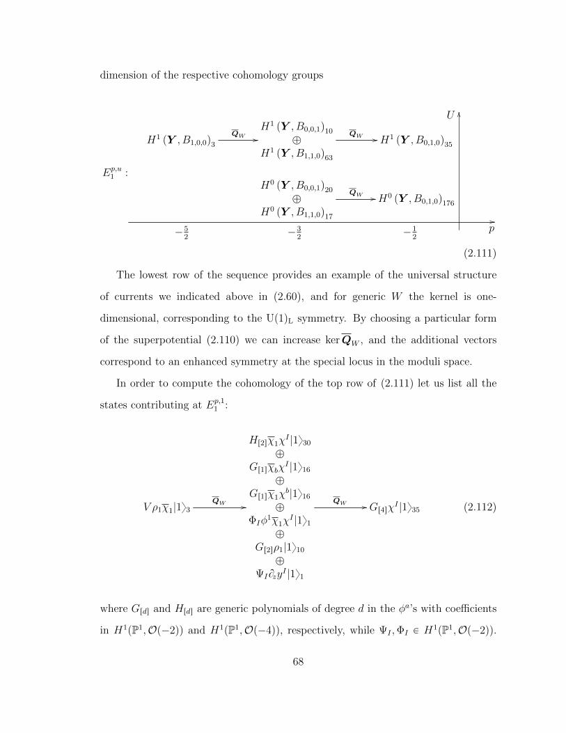
dimension of the respective cohomology groups
Ep,u1 :
H1 pY , B1,0,0q3QW //
H1 pY , B0,0,1q10
‘
H1 pY , B1,1,0q63
QW // H1 pY , B0,1,0q35
H0 pY , B0,0,1q20
‘
H0 pY , B1,1,0q17
QW // H0 pY , B0,1,0q176
//
OO
´32
´52
´12
p
U
(2.111)
The lowest row of the sequence provides an example of the universal structure
of currents we indicated above in (2.60), and for generic W the kernel is one-
dimensional, corresponding to the Up1qL symmetry. By choosing a particular form
of the superpotential (2.110) we can increase kerQW , and the additional vectors
correspond to an enhanced symmetry at the special locus in the moduli space.
In order to compute the cohomology of the top row of (2.111) let us list all the
states contributing at Ep,11 :
V ρ1χ1|1y3QW //
Hr2sχ1χI |1y30
‘
Gr1sχbχI |1y16
‘
Gr1sχ1χb|1y16
‘
ΦIφ1χ1χ
I |1y1‘
Gr2sρ1|1y10
‘
ΨIBzyI |1y1
QW // Gr4sχI |1y35 (2.112)
where Grds and Hrds are generic polynomials of degree d in the φa’s with coefficients
in H1pP1,Op´2qq and H1pP1,Op´4qq, respectively, while ΨI ,ΦI P H1pP1,Op´2qq.
68
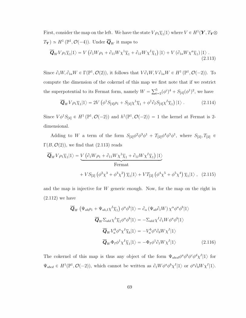
First, consider the map on the left. We have the state V ρ1χ1|1y where V P H1pY , TYb
TY q » H1 pP1,Op´4qq. Under QW it maps to
QWV ρ1χ1|1y “ V`
B1Wρ1 ` B11Wχ1χ1 ` B1IWχIχ1
˘
|1y ` V pB1aWχaχ1q |1y .(2.113)
Since B1W, B1aW P ΓpP1,Op2qq, it follows that V B1W,V B1aW P H1 pP1,Op´2qq. To
compute the dimension of the cokernel of this map we first note that if we restrict
the superpotential to its Fermat form, namely W “ř5i“2pφ
iq4 ` Sr4spφ1q2, we have
QWV ρ1χ1|1y “ 2V`
φ1Sr4sρ1 ` Sr4sχ1χ1 ` φ
1BISr4sχ
Iχ1
˘
|1y . (2.114)
Since V φ1Sr4s P H1 pP1,Op´2qq and h1pP1,Op´2qq “ 1 the kernel at Fermat is 2-
dimensional.
Adding to W a term of the form Sr2sφ2φ3φ1 ` Tr2sφ
4φ5φ1, where Sr2s, Tr2s P
ΓpB,Op2qq, we find that (2.113) reads
QWV ρ1χ1|1y “ V`
B1Wρ1 ` B11Wχ1χ1 ` B1IWχIχ1
˘
|1yloooooooooooooooooooooooooomoooooooooooooooooooooooooon
Fermat
` V Sr2s`
φ2χ3` φ3χ2
˘
χ1|1y ` V Tr2s`
φ4χ5` φ5χ4
˘
χ1|1y , (2.115)
and the map is injective for W generic enough. Now, for the map on the right in
(2.112) we have
QW
`
Ψabρ1 `Ψab,IχIχ1
˘
φaφb|1y “ Bα pΨabB1W qχαφaφb|1y
QWΣabIχIχ1φ
aφb|1y “ ´ΣabIχIB1Wφaφb|1y
QWVba φ
aχIχb|1y “ ´Vba φ
aBbWχI |1y
QWΦIφ1χIχ1|1y “ ´ΦIφ
1B1WχI |1y (2.116)
The cokernel of this map is thus any object of the form ΨabcdφaφbφcφdχI |1y for
Ψabcd P H1pP1,Op´2qq, which cannot be written as B1WφaφbχI |1y or φaBbWχI |1y.
69
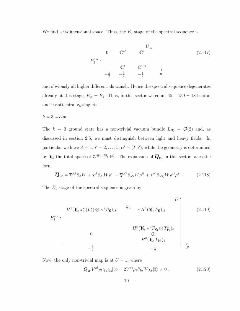
We find a 9-dimensional space. Thus, the E2 stage of the spectral sequence is
Ep,u2 :
0 C45 C9
C1 C139//
OO
´52
´32
´12
p
U
(2.117)
and obviously all higher differentials vanish. Hence the spectral sequence degenerates
already at this stage, E8 “ E2. Thus, in this sector we count 45` 139 “ 184 chiral
and 9 anti-chiral e6-singlets.
k “ 3 sector
The k “ 3 ground state has a non-trivial vacuum bundle L|3y “ Op2q and, as
discussed in section 2.5, we must distinguish between light and heavy fields. In
particular we have A “ 1, i1 “ 2, . . . , 5, α1 “ pI, i1q, while the geometry is determined
by Y3, the total space of O‘4 π3ÝÑ P1. The expansion of QW in this sector takes the
form
QW “ χA:BAW ` χABAiWρi: ` χα1:Bα1iWρi: ` χα
1
Bα1ijWρi:ρj: . (2.118)
The E1 stage of the spectral sequence is given by
Ep,u1 :
H1pY3, π˚3 pL
˚6q b ^
2TY3q18QW // H1pY3, TY3q16
0H0pY3,^
2TY3 b T˚Y3q6
‘
H0pY3, TY3q1 //
OO
´32
´12
p
U
(2.119)
Now, the only non-trivial map is at U “ 1, where
QWVabρ1χaχb|3y “ 2V abρ1B1aWχb|3y ‰ 0 . (2.120)
70
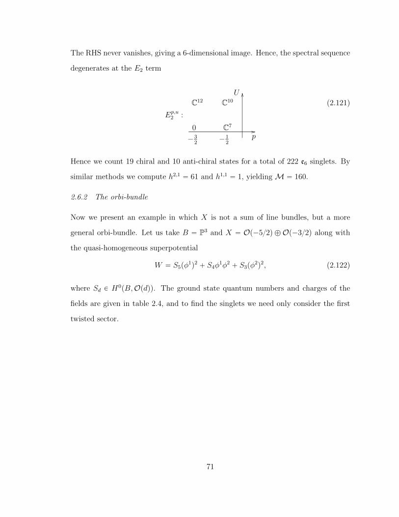
The RHS never vanishes, giving a 6-dimensional image. Hence, the spectral sequence
degenerates at the E2 term
Ep,u2 :
C12 C10
0 C7//
OO
´32
´12
p
U
(2.121)
Hence we count 19 chiral and 10 anti-chiral states for a total of 222 e6 singlets. By
similar methods we compute h2,1 “ 61 and h1,1 “ 1, yielding M “ 160.
2.6.2 The orbi-bundle
Now we present an example in which X is not a sum of line bundles, but a more
general orbi-bundle. Let us take B “ P3 and X “ Op´52q ‘ Op´32q along with
the quasi-homogeneous superpotential
W “ S5pφ1q2` S4φ
1φ2` S3pφ
2q2, (2.122)
where Sd P H0pB,Opdqq. The ground state quantum numbers and charges of the
fields are given in table 2.4, and to find the singlets we need only consider the first
twisted sector.
71
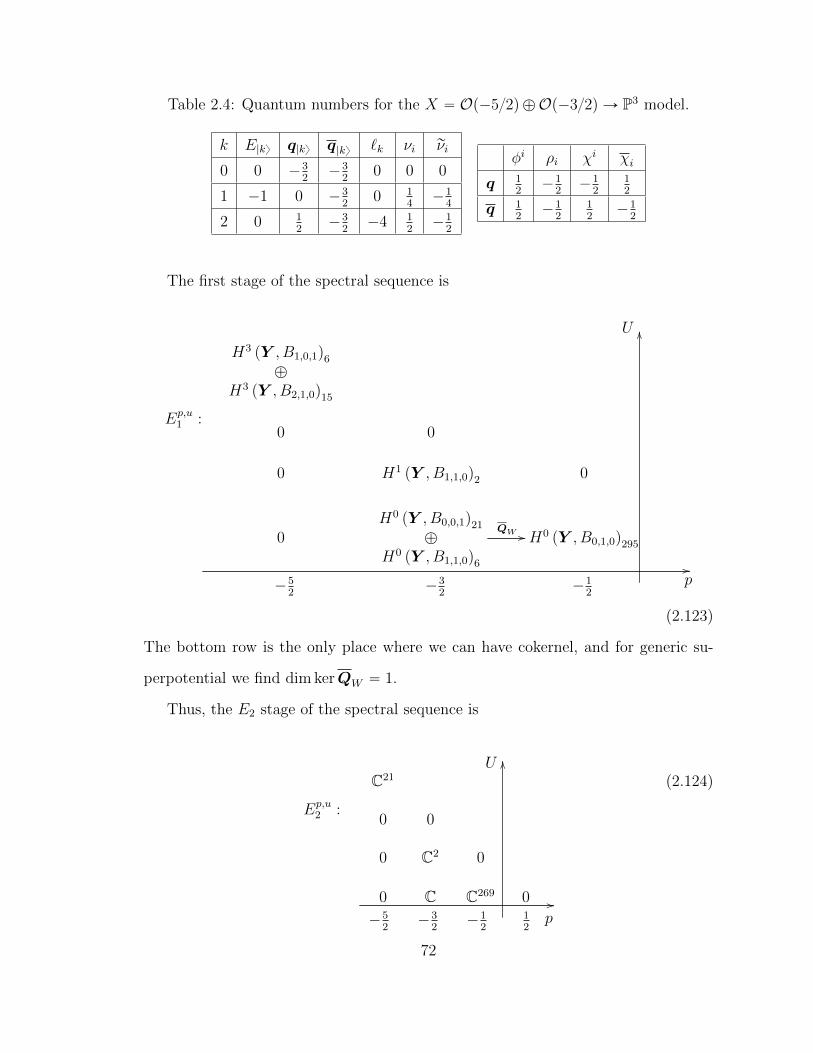
Table 2.4: Quantum numbers for the X “ Op´52q ‘Op´32q Ñ P3 model.
k E|ky q|ky q|ky `k νi rνi
0 0 ´32
´32
0 0 0
1 ´1 0 ´32
0 14
´14
2 0 12
´32
´4 12
´12
φi ρi χi χi
q 12
´12´1
212
q 12
´12
12
´12
The first stage of the spectral sequence is
Ep,u1 :
H3 pY , B1,0,1q6‘
H3 pY , B2,1,0q15
0 0
0 H1 pY , B1,1,0q2 0
0H0 pY , B0,0,1q21
‘
H0 pY , B1,1,0q6
QW // H0 pY , B0,1,0q295
//
OO
´52
´32
´12
p
U
(2.123)
The bottom row is the only place where we can have cokernel, and for generic su-
perpotential we find dim kerQW “ 1.
Thus, the E2 stage of the spectral sequence is
Ep,u2 :
C21
0 0
0 C2 0
0 C C269 0 //
OO
´52
´32
´12
12
p
U(2.124)
72
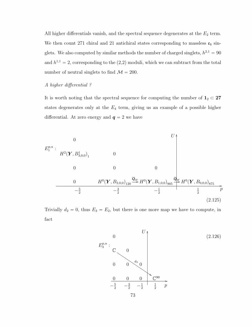
All higher differentials vanish, and the spectral sequence degenerates at the E2 term.
We then count 271 chiral and 21 antichiral states corresponding to massless e6 sin-
glets. We also computed by similar methods the number of charged singlets, h2,1 “ 90
and h1,1 “ 2, corresponding to the (2,2) moduli, which we can subtract from the total
number of neutral singlets to find M “ 200.
A higher differential ?
It is worth noting that the spectral sequence for computing the number of 12 Ă 27
states degenerates only at the E4 term, giving us an example of a possible higher
differential. At zero energy and q “ 2 we have
Ep,u1 :
0
H2pY , B13,0,0q1
0
0 0 0
0 H0pY , B2,0,0q120
QW // H0pY , B1,0,0q905
QW // H0pY , B0,0,0q875 //
OO
´52
´32
´12
12
p
U
(2.125)
Trivially d2 “ 0, thus E3 “ E2, but there is one more map we have to compute, in
fact
Ep,u3 :
0
C
d3
$$
0
0 0 0
0 0 0 C90//
OO
´52
´32
´12
12
p
U(2.126)
73
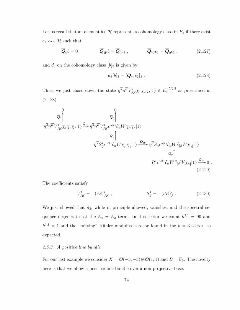
Let us recall that an element b P H represents a cohomology class in E3 if there exist
c1, c2 P H such that
Q0b “ 0 , QW b “ Q0c1 , QW c1 “ Q0c2 , (2.127)
and d3 on the cohomology class rbs3 is given by
d3rbs3 “ rQW c2s3 . (2.128)
Thus, we just chase down the state ηJηKV IJKχ1χ2χI |1y P E
´52,33 as prescribed in
(2.128)
0 0
ηJηKV IJKχ1χ2χI |1y
QW //
Q0
OO
ηJηKV IJKεαβγBαWχβχγ|1y
Q0
OO
ηJSIJεαβγBαWχβχγ|1y
Q0
OO
QW // ηJSIJεαβγBαWBrβWχγs|1y
RIεαβγBαWBrβWχγs|1y
Q0
OO
QW // 0 .
(2.129)
The coefficients satisfy
V IJK“ ´pBSqI
JK, SI
J“ ´pBRqI
J. (2.130)
We just showed that d3, while in principle allowed, vanishes, and the spectral se-
quence degenerates at the E4 “ E2 term. In this sector we count h2,1 “ 90 and
h1,1 “ 1 and the “missing” Kahler modulus is to be found in the k “ 3 sector, as
expected.
2.6.3 A positive line bundle
For our last example we consider X “ Op´3,´3q‘Op1, 1q and B “ F0. The novelty
here is that we allow a positive line bundle over a non-projective base.
74
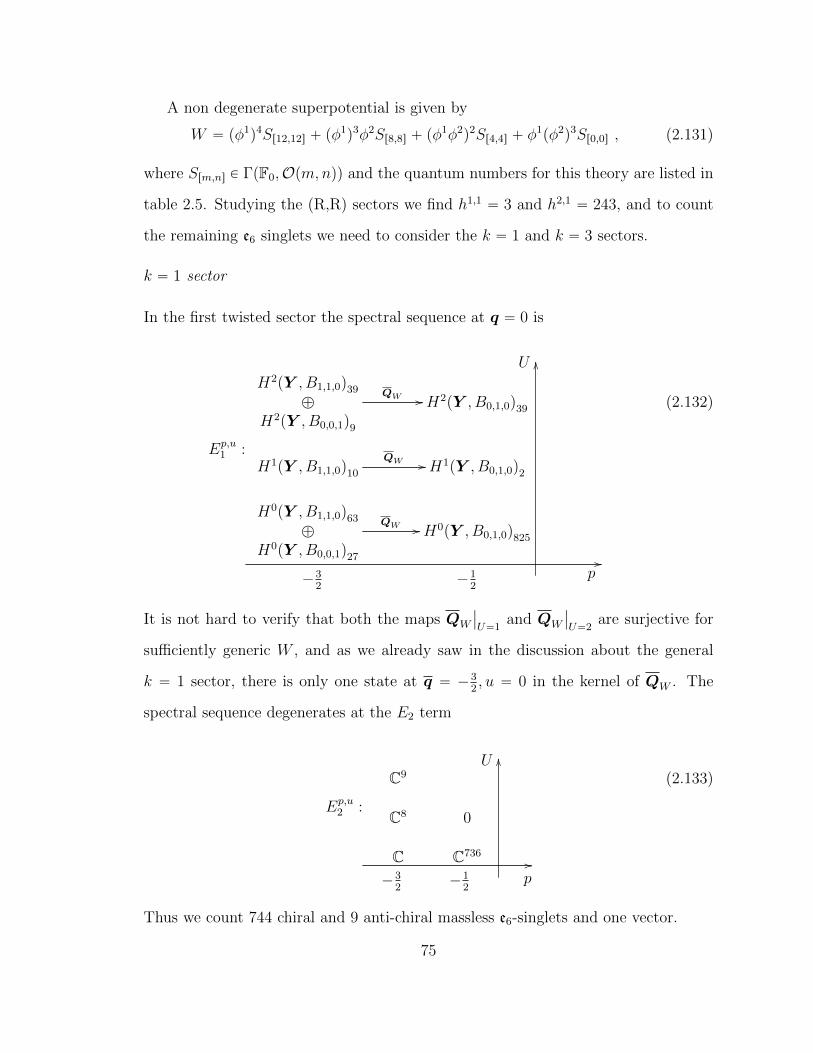
A non degenerate superpotential is given by
W “ pφ1q4Sr12,12s ` pφ
1q3φ2Sr8,8s ` pφ
1φ2q2Sr4,4s ` φ
1pφ2q3Sr0,0s , (2.131)
where Srm,ns P ΓpF0,Opm,nqq and the quantum numbers for this theory are listed in
table 2.5. Studying the (R,R) sectors we find h1,1 “ 3 and h2,1 “ 243, and to count
the remaining e6 singlets we need to consider the k “ 1 and k “ 3 sectors.
k “ 1 sector
In the first twisted sector the spectral sequence at q “ 0 is
Ep,u1 :
H2pY , B1,1,0q39
‘
H2pY , B0,0,1q9
QW // H2pY , B0,1,0q39
H1pY , B1,1,0q10
QW // H1pY , B0,1,0q2
H0pY , B1,1,0q63
‘
H0pY , B0,0,1q27
QW // H0pY , B0,1,0q825
//
OO
p
U
´32
´12
(2.132)
It is not hard to verify that both the maps QW
ˇ
ˇ
U“1and QW
ˇ
ˇ
U“2are surjective for
sufficiently generic W , and as we already saw in the discussion about the general
k “ 1 sector, there is only one state at q “ ´32, u “ 0 in the kernel of QW . The
spectral sequence degenerates at the E2 term
Ep,u2 :
C9
C8 0
C C736//
OO
p
U
´32
´12
(2.133)
Thus we count 744 chiral and 9 anti-chiral massless e6-singlets and one vector.
75
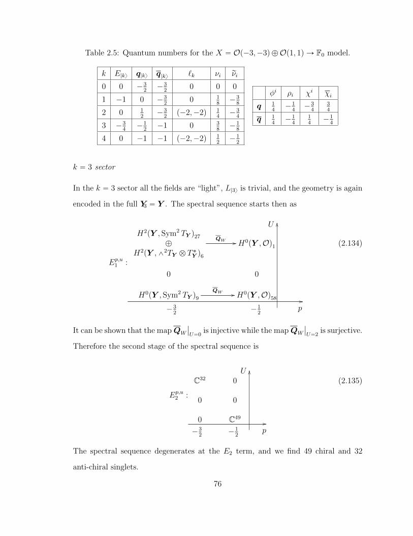
Table 2.5: Quantum numbers for the X “ Op´3,´3q ‘Op1, 1q Ñ F0 model.
k E|ky q|ky q|ky `k νi rνi
0 0 ´32
´32
0 0 0
1 ´1 0 ´32
0 18
´38
2 0 12
´32
p´2,´2q 14
´34
3 ´34
´12
´1 0 38
´18
4 0 ´1 ´1 p´2,´2q 12
´12
φi ρi χi χi
q 14
´14´3
434
q 14
´14
14
´14
k “ 3 sector
In the k “ 3 sector all the fields are “light”, L|3y is trivial, and the geometry is again
encoded in the full Y3 “ Y . The spectral sequence starts then as
Ep,u1 :
H2pY , Sym2 TY q27
‘
H2pY ,^2TY b T˚Y q6
QW // H0pY ,Oq1
0 0
H0pY , Sym2 TY q9QW // H0pY ,Oq58 //
OO
´32
´12
p
U
(2.134)
It can be shown that the mapQW
ˇ
ˇ
U“0is injective while the mapQW
ˇ
ˇ
U“2is surjective.
Therefore the second stage of the spectral sequence is
Ep,u2 :
C32 0
0 0
0 C49//
OO
p
U
´32
´12
(2.135)
The spectral sequence degenerates at the E2 term, and we find 49 chiral and 32
anti-chiral singlets.
76
Summarizing, we count 834 massless chiral e6-singlets and once we subtract the
moduli we obtain M “ 588.
2.7 Discussion
We have described a class of perturbative vacua for heterotic string compactifications
and a limit in which their properties are computable. We have illustrated these
computations in models with (2,2) world-sheet supersymmetry, although the methods
clearly extend to more general (0,2) theories.
Our class of (2,2) models fits in with a number of other constructions. To describe
this we proceed in increasing dimension d of the base B and assume this is Fano.
For d “ 1 this means B “ P1 and the c “ 6 LGO theory on the fiber determines a
one-parameter family of K3 compactifications. Models with no large radius limit in
the Kahler moduli space, such as the first example in section 2.6, are obtained when
the monodromies of the family are not simultaneously geometrical in any duality
frame. It seems likely that any such model would be obtained as a limit in some
GLSM, but we have not shown this.
For d “ 2 the base is a del Pezzo surface and the c “ 3 LGO theory on the fiber
can be interpreted as determining in Weierstrass form an elliptic fibration over B.
This can be smooth if the discriminant is nonsingular in B, in which case the model
will have a large-radius limit. It is not clear how to construct a GLSM embedding
for a hybrid with a non-toric base.
For d “ 3 there are many possible choices for B, but the c “ 0 LGO theory
is quadratic, and hence appears to be trivial. Since the fiber fields are massive at
generic points on the base, one might think the low-energy theory would be a NLSM
with target space B, but this cannot be correct, as this would not be conformally
invariant. This naıve discussion omits the orbifold action. Since at low energy there
are no excitations in the fiber direction, one can try [2] to describe the resulting
77
model as a NLSM with target space a double cover of B branched over the singular
locus of W py, φq considered as a function of φ only . This leads to a geometric
interpretation of the limiting point we called the hybrid limit. It is not directly
related to a symplectic quotient construction and, if the model has a large-radius
limit, it is not birational to the target space at this limit. The relationship between
the two descriptions is unclear. It would be interesting to study, among other things,
the behavior of the D-brane spectrum and moduli in a type-IIA compactification
near such a hybrid limit.
The models we have studied have been “good” hybrids, in which the R-symmetry
does not act on the base. Limiting points of GLSMs often produce hybrids for which
this does not hold. The hybrid limit for “good” hybrids is expected to lie at infi-
nite distance in the moduli space of SCFTs; it should be possible to determine the
approximate moduli space metric in the hybrid limit. We expect that the approx-
imation should improve as the hybrid limit is approached and the distance to the
hybrid limit deep in the Kahler cone of B will diverge. It would be interesting to
verify this in detail. In [8] “pseudo” hybrids were defined as hybrid limits lying at
finite distance; the behavior of the D-brane spectrum near these limits was found
to be quite different from that expected near a “good” hybrid. It seems natural to
conjecture that “good” hybrids and “true” (not “pseudo”) hybrid limits coincide.
Although we focused on models with (2,2) world-sheet supersymmetry, the meth-
ods extend naturally to a much larger class of models with (0,2) supersymmetry. This
larger class presents an array of interesting questions. As a first foray in this direc-
tion, the massless e6 singlets in (NS,R) sectors belong to (anti-) chiral multiplets
containing massless scalars. Expectation values for these represent marginal defor-
mations of the world-sheet SCFT preserving (0,2) supersymmetry. We do not at
present have effective techniques to determine which of these are exactly marginal,
and the structure of the moduli space of (0,2) SCFTs is still largely unknown.
78
In general one expects [35, 40] that away from the hybrid limit the (0,2) models
we construct will be destabilized by world-sheet instantons wrapping cycles in B. In
some classes of models this expectation has been thwarted, and the anticipated cor-
rections are absent [91, 16, 17]. Even in cases in which no known argument precludes
such corrections they have been found less generally than one might expect [11, 7].
It would be very interesting to investigate this issue in the context of hybrid models,
in which the structure of the relevant instantons – associated to rational curves in
B rather than in a Calabi–Yau threefold, may provide a simpler context for their
study.
More generally, we can construct (0,2) hybrid models that are not deformations
of (2,2) models by taking the left-moving fermions to be sections of a holomorphic
bundle E Ñ Y and a (0,2) superpotential given by a section J P ΓpE˚q with J´1p0q “
B. It is to be expected that most such models will not have a limit in which they
are described by a (0,2) NLSM or one in which they reduce to a (0,2) LGO theory,
so that these will determine a large class of new perturbative vacua of the heterotic
string.
79
3
Accidents in (0,2) Landau-Ginzburg models
3.1 Introduction
The construction and classification of conformal field theories (CFTs) plays a key role
in modern quantum field theory. One approach is to solve the conformal bootstrap.1
Another approach that has proven useful is to study the low energy (or IR) limits of
renormalization group (RG) flows from known CFTs. This has challenges of its own,
since the IR dynamics often involves emergent degrees of freedom and interactions.
Nevertheless, as already indicated in the seminal work of [100, 63, 75, 93], it is
often possible to identify certain classes of operators and their OPEs and correlators
of an IR CFT with corresponding objects in terms of the UV degrees of freedom. This
is especially useful when the UV theory is asymptotically free, since then perturbative
computations can provide information about a non-trivial CFT without a notion of
a weak coupling. The identification of UV and IR data is simplified when some
amount of supersymmetry is preserved along the RG flow: SUSY constraints lead to
1 This is difficult in practice and can be carried out analytically only in theories with enormouslyenlarged symmetries like the WN algebras of the minimal models [22]. Recently progress hasbeen made with numeric techniques, for example in applications to the three-dimensional Isingmodel [48, 47].
80
well-known simplifications such as the relation between dimensions and R-charges of
chiral operators and non-renormalization theorems. For instance, in two dimensional
theories with (2,2) SUSY these simplifications are responsible for many well-known
phenomena such as mirror symmetry and the Calabi-Yau (CY) / Landau-Ginzburg
(LG) correspondence [56], and the identification of UV and IR data is a key tool in
exploration and exploitation of these two-dimensional gems.
Such techniques rely on the assumption that accidental symmetries that might
emerge in the IR limit do not invalidate the identification of operators in the IR with
their UV avatars. This assumption is well-tested in (2,2) theories but is also often
applied to theories with only (0,2) supersymmetry. For instance, it is key to various
gauged linear sigma model constructions of (0,2) CFTs corresponding to heterotic
string vacua [97, 41, 91, 39].
In this chapter we show that the assumption cannot be taken for granted in
(0,2) theories, and the resulting “accidents” have drastic consequences for the IR
physics and the relation between UV parameters and IR data. The examples we
consider are (0,2) Landau-Ginzburg theories, and we identify a class of accidental
symmetries of (0,2) LG RG flows by studying the space of F-term UV couplings
modulo field redefinitions. We find that these accidental symmetries significantly
modify the analysis of the IR theory. For instance, the spectrum of chiral operators
and even the IR central charge are in general modified. This invalidates certain UV
theories from giving good models for (0,2) SCFTs appropriate for a heterotic string
vacuum—we examine an example taken from [41].
A classic (2,2) example
To describe the challenges of (0,2) accidents more precisely, it is useful to review
the successes of the (2,2) theories. Consider the quintic (2,2) LG model with chiral
81
superpotential
W “ α0X50 ` α1X
51 ` ¨ ¨ ¨ ` α4X
54 ´ 5α5X0X1 ¨ ¨ ¨X4 .
Here the Xi are (2,2) chiral superfields and the αa are complex parameters. This
theory flows to a c “ c “ 9 (2,2) SCFT.2 The complex parameter
ψ “ α55pα0α1 ¨ ¨ ¨α4q
´1
is invariant under C˚ rescalings of the chiral superfieldsXi and labels a one-parameter
family of IR CFTs. At generic values of ψ the IR fixed point is a well-behaved CFT,
and small changes in ψ correspond to small marginal deformations of the CFT, where
“small” refers to the distance in the Zamolodchikov metric. At special values of ψ
the CFT can become singular. For instance, ψ “ 1 is a finite distance singularity
—the analogue of a conifold point. This can be detected in the UV description: the
theory develops a family of supersymmetric vacua with Xi “ const., and these signal
a non-compact CFT: a theory with a continuum spectrum of conformal dimensions.
Another point, ψ “ 8 is an infinite-distance singularity.
The quotient of the UV parameter space by field redefinitions is a complicated
object [9, 33] with singularities and non-separated points. For instance, we can take
the limit α0 Ñ 0 and α5 Ñ 0 while keeping ψ constant so as to obtain a product of
four minimal models coupled to a free chiral superfield X0, with c “ c “ 3p3 ` 25q.
Fortunately, all such bad points are singular CFTs. The bad points corresponding to
various infinite distance singularities and “wrong” central charges are easily identified
in terms of the UV data: they all correspond to singular superpotentials with a
continuum of supersymmetric vacua and therefore a continuum of states in the IR
CFT. Away from such points the quotient is sensible and describes (2,2) marginal
deformations of the IR theory.
2 A Z5 orbifold of the theory describes a (2,2) non-linear sigma model with target space the quinticCY hypersurface in P4 at a special value of the complexified Kahler parameter. A complex structureparameter of the geometry is then related to the LG parameter ψ.
82
Similar considerations apply to more general (2,2) gauged linear sigma models,
and with the parametrization of the smooth CFTs in terms of the UV parameters
in hand, localization and topological field theory techniques can be used to compute
certain correlators and chiral spectra in the CFT in terms of the weakly coupled UV
Lagrangian.
(0,2) challenges
As we will show in section 3.3, the situation is more delicate in (0,2) theories, even
in the relatively simple class of LG models (we review these in section 3.2). The
essential difference is that we lack the simple diagnostic we had for a “bad” point in
(2,2) theories. It is not sufficient to exclude UV parameters that lead to flat directions
in the potential, and the identification of UV parameters with marginal deformations
of the CFT requires (at least) a study of loci with enhanced symmetry. Unlike in
(2,2) examples, accidental symmetries can emerge for non-singular UV potentials,
thereby complicating the description of IR physics in terms of the UV data. Unlike
in (2,2) theories a family of smooth UV potentials with each potential preserving
the same R-symmetry along the RG flow need not correspond to a family of CFTs
related by truly marginal deformations.
Fortunately, at least in (0,2) LG models it appears that we have enough control
to identify accidental symmetries and special loci in the parameter space by gen-
eralizing the (2,2) paradigm of parametrizing the IR fixed points by the space of
UV parameters modulo field redefinitions. This uncovers a rich structure of (0,2)
RG flows and of the space of marginal deformations of (0,2) fixed points and will
undoubtedly play a role in quantitatively descriptions of (0,2) moduli spaces.
Once we have identified a (0,2) LG theory with some particular IR fixed point, it
is useful to develop the correspondence between deformations of the UV Lagrangian
and (0,2) conformal perturbation theory. In section 3.4 we describe some properties
83
of (0,2) conformal perturbation theory independent of any embedding of the CFT in
a critical heterotic string. This section can be read independently from the rest of
the chapter. We use these observations in section 3.5 to describe a conjecture for the
global structure of the moduli space of (0,2) SCFTs with expected central charge in
terms of the UV data for what we term plain (0,2) LG models.
3.2 A glance at (0,2) Landau-Ginzburg theories
We begin with a quick review of (0,2) LG theories following [41, 66, 79].3 We work
in Euclidean signature and a (0,2) superspace with coordinates pz, z, θ, θq. The UV
theory consists of n bosonic chiral multiplets Φi “ φi ` . . . , and N fermionic chiral
multiplets ΓA “ γA` . . ., as well as their conjugate anti-chiral multiplets. These are
given a free kinetic term and a (0,2) SUSY potential term as interactions:
Lint “
ż
dθ W ` h.c. , W “ m0
ř
A ΓAJApΦq , (3.1)
where m0 has mass dimension 1 and the JA are polynomial in the Φi. This is the
simplest example of a (0,2) SUSY asymptotically free theory: for energies E " m0
the theory is well-described by the set of free fields. Conversely, when E ! m0 the
interactions become important and lead to non-trivial IR dynamics that depend on
n,N , as well as the choice of ideal J “ xJ1, . . . , JNy Ă CrΦ1, . . . ,Φns. What can we
say about the IR limit of this theory?
A basic constraint comes from the gravitational anomaly. In the UV the central
charges are easy to determine: each Φ multiplet contains a complex boson and a
right-moving Weyl fermion, while each Γ contains a left-moving Weyl fermion and
an auxiliary field. Hence, we have cUV “ 2n`N , cUV “ 3n. The RG flow induced by
W will decrease the central charges, but since it is Lorentz-invariant, it will preserve
the difference c´ c “ N ´ n.
3 Our superspace conventions are those of [79].
84
Another basic property of the theory is the set of global symmetries. The free
theory has a large global symmetry that commutes with (0,2) SUSY: namely, Upnqˆ
UpNq rotations of the chiral superfields. In addition we have the R-symmetry that
rotates θ and leaves the lowest components of the superfields φi and γA invariant.
The interactions break these symmetries. For completely generic JA the remaining
symmetry just Up1q0R – an R-symmetry that assigns charge `1 to θ and γA and
charge 0 to φi.
Properties of the superpotential
A key feature of (0,2) LG theories is that the holomorphic superpotential obeys
the same non-renormalization properties as the, perhaps more familiar N=1 d=4
Wess-Zumino model’s superpotential. The kinetic term, on the other hand, is a
full superspace derivative and will receive complicated corrections along the RG
flow. However, just as in (2,2) theories, we expect these corrections to be irrelevant
provided that the fields Φ and Γ all acquire non-trivial scaling dimensions. In order
to relate these scaling dimensions to properties of the UV theory, we will assume
that the interactions preserve an additional global Up1q symmetry, which we will call
Up1qL, under which ΓA have charges QA, while the Φi carry charges qi. This will be
the case if and only if the ideal is quasi-homogeneous, i.e.
JAptqiΦiq “ t´QAJApΦq (3.2)
for all t P C˚. We will demand that the ideal is zero-dimensional, i.e. JApΦq “ 0 for
all A if and only if Φ “ 0. If it is not then the theory necessarily has a non-compact
set of supersymmetric vacua labeled by vevs of the bosonic fields. We will call such
superpotentials singular. We are interested in “compact” CFTs and exclude this
possibility.4
4 A CFT is compact if its spectrum is such that for every fixed real ∆ there is a finite number offields with dimension less than ∆.
85
Another important property of the superpotential is that typically some of its
parameters are not, in fact, F-terms. To see this, consider a perturbation of the form
δW “ř
A ΓAδJA around a theory with W0 “ř
A ΓAJA. In the undeformed theory,
if we assume canonical kinetic terms, the equations of motion read
DΓA“ JApΦq , DBzΦi “
ÿ
A
ΓABJABΦi
, (3.3)
where D is the antichiral superspace derivative D “ Bθ` θBz. A more general kinetic
term leads to more complicated expressions under the D derivative of the left-hand
sides of the equations.5 Hence, a first order deformation of W of the form
δJA “ÿ
B
MBA pΦqJBpΦq `
ÿ
i
BJABΦi
FipΦq (3.4)
is equivalent up to equations of motion to a D-term deformation.
The LG assumption that the D-terms are irrelevant along the flow implies that
any two UV theories with superpotentials related by a holomorphic field redefinition
lead to the same IR fixed point. Hence, any two UV superpotentials that are related
by a holomorphic field redefinition belong to the same universality class.
(2,2) LG theories
The (0,2) theory will have an enhanced left-moving SUSY when N “ n, so that
in the free limit we can combine pΓi,Φiq into (2,2) chiral multiplets X i, and when
Ji “ BW BΦi for some potential W . In that case, we can rewrite the theory in a
manifestly (2,2) supersymmetric fashion with a chiral superpotential W pXq. The
quasi-homogeneity conditions set Qi “ qi ´ 1, and the resulting central charge is
given by the famous
c “ 3ÿ
i
p1´ 2qiq . (3.5)
5 In a NLSM such total derivatives are more subtle than in this LG setting, as they are usuallyonly sensible patch by patch in target space. Indeed, marginal deformations of NLSMs are suchF-terms that cannot be globally recast as D-terms [18, 81].
86
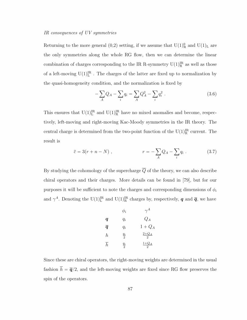
IR consequences of UV symmetries
Returning to the more general (0,2) setting, if we assume that Up1q0R and Up1qL are
the only symmetries along the whole RG flow, then we can determine the linear
combination of charges corresponding to the IR R-symmetry Up1qIRR as well as those
of a left-moving Up1qIRL . The charges of the latter are fixed up to normalization by
the quasi-homogeneity condition, and the normalization is fixed by
´ÿ
A
QA ´ÿ
i
qi “ÿ
A
Q2A ´
ÿ
i
q2i . (3.6)
This ensures that Up1qIRL and Up1qIRR have no mixed anomalies and become, respec-
tively, left-moving and right-moving Kac-Moody symmetries in the IR theory. The
central charge is determined from the two-point function of the Up1qIRR current. The
result is
c “ 3pr ` n´Nq , r “ ´ÿ
A
QA ´ÿ
i
qi . (3.7)
By studying the cohomology of the supercharge Q of the theory, we can also describe
chiral operators and their charges. More details can be found in [79], but for our
purposes it will be sufficient to note the charges and corresponding dimensions of φi
and γA. Denoting the Up1qIRL and Up1qIRR charges by, respectively, q and q, we have
φi γA
q qi QA
q qi 1`QA
h qi2
2`QA2
h qi2
1`QA2
Since these are chiral operators, the right-moving weights are determined in the usual
fashion h “ q2, and the left-moving weights are fixed since RG flow preserves the
spin of the operators.
87
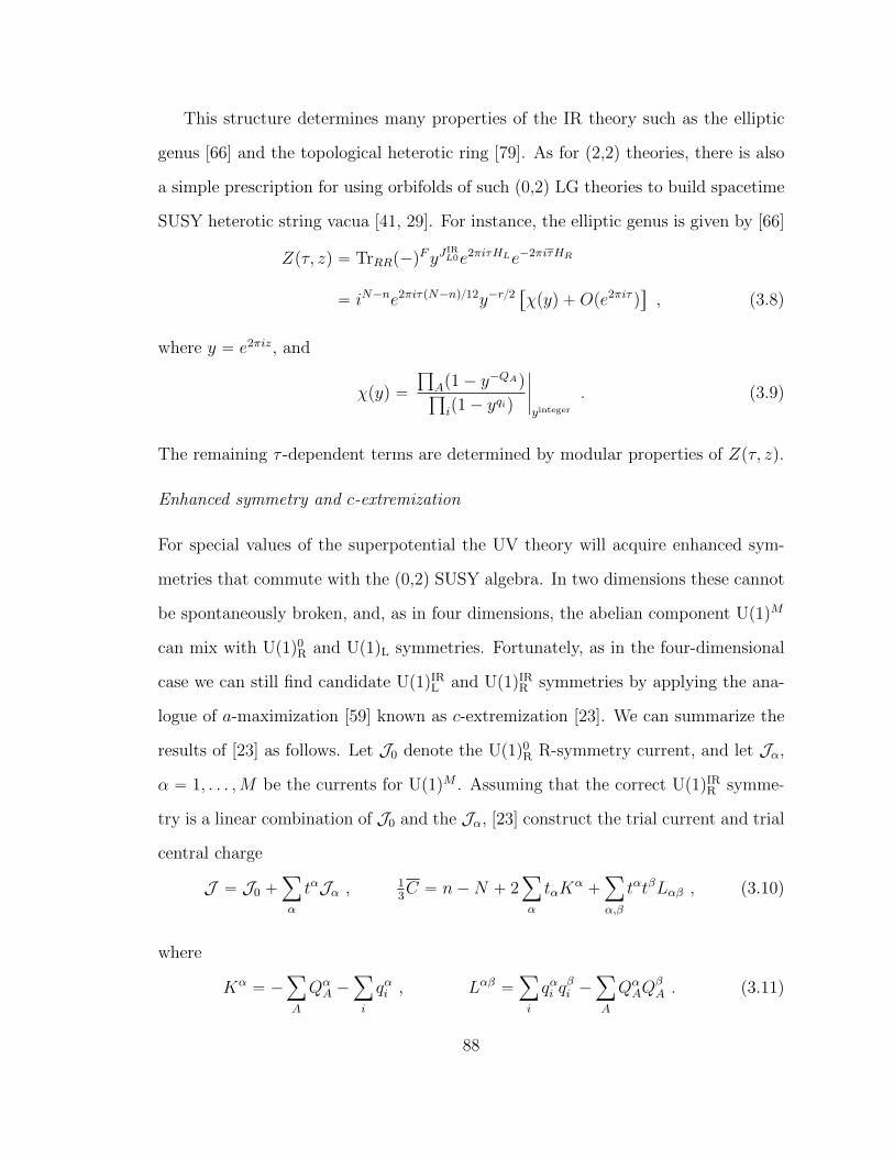
This structure determines many properties of the IR theory such as the elliptic
genus [66] and the topological heterotic ring [79]. As for (2,2) theories, there is also
a simple prescription for using orbifolds of such (0,2) LG theories to build spacetime
SUSY heterotic string vacua [41, 29]. For instance, the elliptic genus is given by [66]
Zpτ, zq “ TrRRp´qFyJ
IRL0e2πiτHLe´2πiτHR
“ iN´ne2πiτpN´nq12y´r2“
χpyq `Ope2πiτq‰
, (3.8)
where y “ e2πiz, and
χpyq “
ś
Ap1´ y´QAq
ś
ip1´ yqiq
ˇ
ˇ
ˇ
ˇ
yinteger
. (3.9)
The remaining τ -dependent terms are determined by modular properties of Zpτ, zq.
Enhanced symmetry and c-extremization
For special values of the superpotential the UV theory will acquire enhanced sym-
metries that commute with the (0,2) SUSY algebra. In two dimensions these cannot
be spontaneously broken, and, as in four dimensions, the abelian component Up1qM
can mix with Up1q0R and Up1qL symmetries. Fortunately, as in the four-dimensional
case we can still find candidate Up1qIRL and Up1qIRR symmetries by applying the ana-
logue of a-maximization [59] known as c-extremization [23]. We can summarize the
results of [23] as follows. Let J0 denote the Up1q0R R-symmetry current, and let Jα,
α “ 1, . . . ,M be the currents for Up1qM . Assuming that the correct Up1qIRR symme-
try is a linear combination of J0 and the Jα, [23] construct the trial current and trial
central charge
J “ J0 `ÿ
α
tαJα , 13C “ n´N ` 2
ÿ
α
tαKα`ÿ
α,β
tαtβLαβ , (3.10)
where
Kα“ ´
ÿ
A
QαA ´
ÿ
i
qαi , Lαβ “ÿ
i
qαi qβi ´
ÿ
A
QαAQ
βA . (3.11)
88
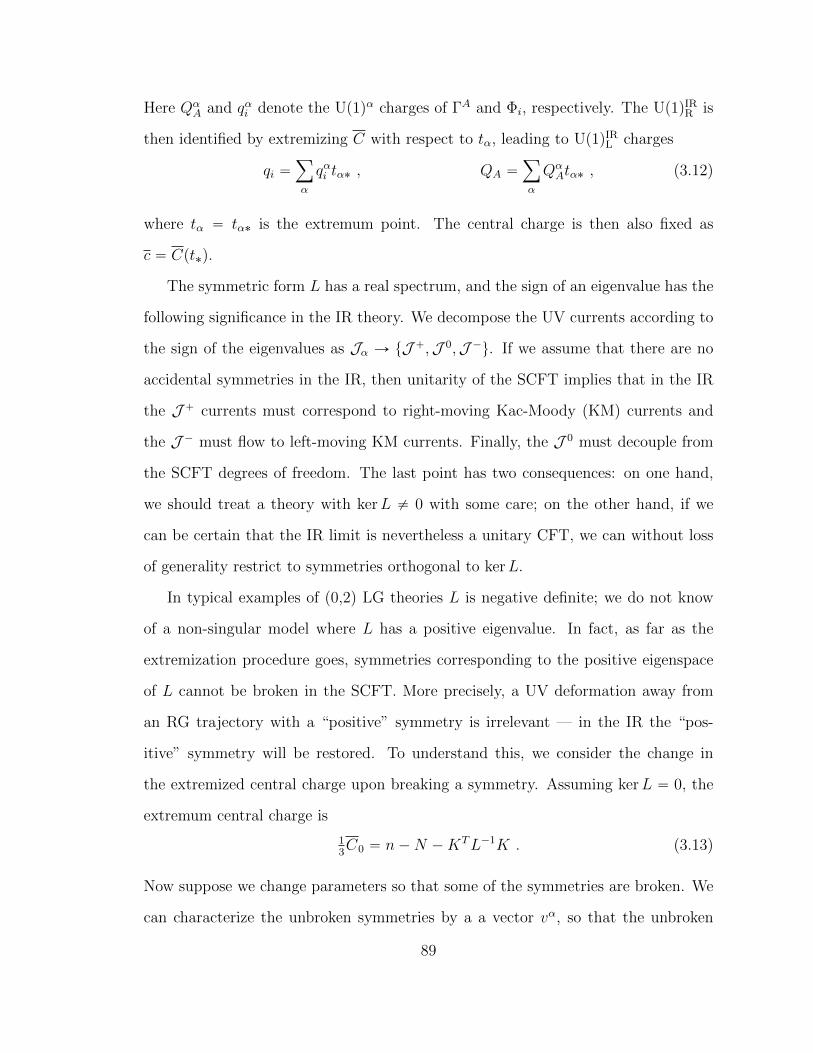
Here QαA and qαi denote the Up1qα charges of ΓA and Φi, respectively. The Up1qIRR is
then identified by extremizing C with respect to tα, leading to Up1qIRL charges
qi “ÿ
α
qαi tα˚ , QA “ÿ
α
QαAtα˚ , (3.12)
where tα “ tα˚ is the extremum point. The central charge is then also fixed as
c “ Cpt˚q.
The symmetric form L has a real spectrum, and the sign of an eigenvalue has the
following significance in the IR theory. We decompose the UV currents according to
the sign of the eigenvalues as Jα Ñ tJ `,J 0,J ´u. If we assume that there are no
accidental symmetries in the IR, then unitarity of the SCFT implies that in the IR
the J ` currents must correspond to right-moving Kac-Moody (KM) currents and
the J ´ must flow to left-moving KM currents. Finally, the J 0 must decouple from
the SCFT degrees of freedom. The last point has two consequences: on one hand,
we should treat a theory with kerL ‰ 0 with some care; on the other hand, if we
can be certain that the IR limit is nevertheless a unitary CFT, we can without loss
of generality restrict to symmetries orthogonal to kerL.
In typical examples of (0,2) LG theories L is negative definite; we do not know
of a non-singular model where L has a positive eigenvalue. In fact, as far as the
extremization procedure goes, symmetries corresponding to the positive eigenspace
of L cannot be broken in the SCFT. More precisely, a UV deformation away from
an RG trajectory with a “positive” symmetry is irrelevant — in the IR the “pos-
itive” symmetry will be restored. To understand this, we consider the change in
the extremized central charge upon breaking a symmetry. Assuming kerL “ 0, the
extremum central charge is
13C0 “ n´N ´KTL´1K . (3.13)
Now suppose we change parameters so that some of the symmetries are broken. We
can characterize the unbroken symmetries by a a vector vα, so that the unbroken
89
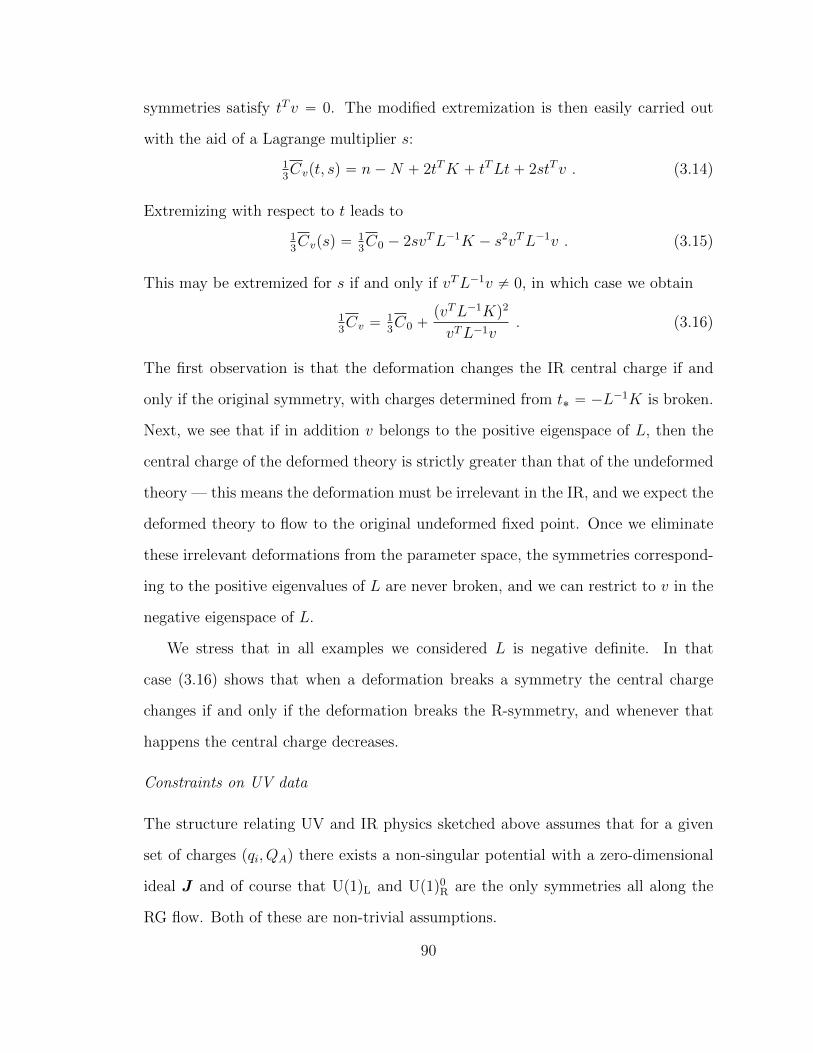
symmetries satisfy tTv “ 0. The modified extremization is then easily carried out
with the aid of a Lagrange multiplier s:
13Cvpt, sq “ n´N ` 2tTK ` tTLt` 2stTv . (3.14)
Extremizing with respect to t leads to
13Cvpsq “
13C0 ´ 2svTL´1K ´ s2vTL´1v . (3.15)
This may be extremized for s if and only if vTL´1v ‰ 0, in which case we obtain
13Cv “
13C0 `
pvTL´1Kq2
vTL´1v. (3.16)
The first observation is that the deformation changes the IR central charge if and
only if the original symmetry, with charges determined from t˚ “ ´L´1K is broken.
Next, we see that if in addition v belongs to the positive eigenspace of L, then the
central charge of the deformed theory is strictly greater than that of the undeformed
theory — this means the deformation must be irrelevant in the IR, and we expect the
deformed theory to flow to the original undeformed fixed point. Once we eliminate
these irrelevant deformations from the parameter space, the symmetries correspond-
ing to the positive eigenvalues of L are never broken, and we can restrict to v in the
negative eigenspace of L.
We stress that in all examples we considered L is negative definite. In that
case (3.16) shows that when a deformation breaks a symmetry the central charge
changes if and only if the deformation breaks the R-symmetry, and whenever that
happens the central charge decreases.
Constraints on UV data
The structure relating UV and IR physics sketched above assumes that for a given
set of charges pqi, QAq there exists a non-singular potential with a zero-dimensional
ideal J and of course that Up1qL and Up1q0R are the only symmetries all along the
RG flow. Both of these are non-trivial assumptions.
90
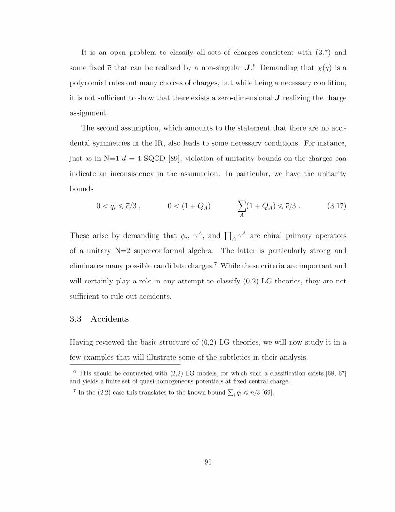
It is an open problem to classify all sets of charges consistent with (3.7) and
some fixed c that can be realized by a non-singular J .6 Demanding that χpyq is a
polynomial rules out many choices of charges, but while being a necessary condition,
it is not sufficient to show that there exists a zero-dimensional J realizing the charge
assignment.
The second assumption, which amounts to the statement that there are no acci-
dental symmetries in the IR, also leads to some necessary conditions. For instance,
just as in N=1 d “ 4 SQCD [89], violation of unitarity bounds on the charges can
indicate an inconsistency in the assumption. In particular, we have the unitarity
bounds
0 ă qi ď c3 , 0 ă p1`QAqÿ
A
p1`QAq ď c3 . (3.17)
These arise by demanding that φi, γA, and
ś
A γA are chiral primary operators
of a unitary N=2 superconformal algebra. The latter is particularly strong and
eliminates many possible candidate charges.7 While these criteria are important and
will certainly play a role in any attempt to classify (0,2) LG theories, they are not
sufficient to rule out accidents.
3.3 Accidents
Having reviewed the basic structure of (0,2) LG theories, we will now study it in a
few examples that will illustrate some of the subtleties in their analysis.
6 This should be contrasted with (2,2) LG models, for which such a classification exists [68, 67]and yields a finite set of quasi-homogeneous potentials at fixed central charge.
7 In the (2,2) case this translates to the known boundř
i qi ď n3 [69].
91
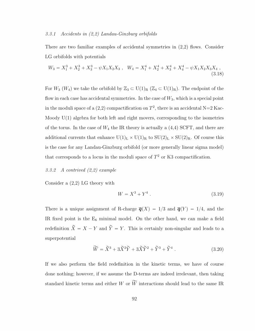
3.3.1 Accidents in (2,2) Landau-Ginzburg orbifolds
There are two familiar examples of accidental symmetries in (2,2) flows. Consider
LG orbifolds with potentials
W3 “ X31 `X
32 `X
33 ´ ψX1X2X3 , W4 “ X4
1 `X42 `X
43 `X
44 ´ ψX1X2X3X4 ,
(3.18)
For W3 (W4) we take the orbifold by Z3 Ă Up1qR (Z4 Ă Up1qR). The endpoint of the
flow in each case has accidental symmetries. In the case ofW3, which is a special point
in the moduli space of a (2,2) compactification on T 2, there is an accidental N=2 Kac-
Moody Up1q algebra for both left and right movers, corresponding to the isometries
of the torus. In the case of W4 the IR theory is actually a (4,4) SCFT, and there are
additional currents that enhance Up1qL ˆUp1qR to SUp2qL ˆ SUp2qR. Of course this
is the case for any Landau-Ginzburg orbifold (or more generally linear sigma model)
that corresponds to a locus in the moduli space of T 2 or K3 compactification.
3.3.2 A contrived (2,2) example
Consider a (2,2) LG theory with
W “ X3` Y 4 . (3.19)
There is a unique assignment of R-charge qpXq “ 13 and qpY q “ 14, and the
IR fixed point is the E6 minimal model. On the other hand, we can make a field
redefinition rX “ X ´ Y and rY “ Y . This is certainly non-singular and leads to a
superpotential
ĂW “ rX3` 3 rX2
rY ` 3 rX rY 2` rY 3
` rY 4 . (3.20)
If we also perform the field redefinition in the kinetic terms, we have of course
done nothing; however, if we assume the D-terms are indeed irrelevant, then taking
standard kinetic terms and either W or ĂW interactions should lead to the same IR
92
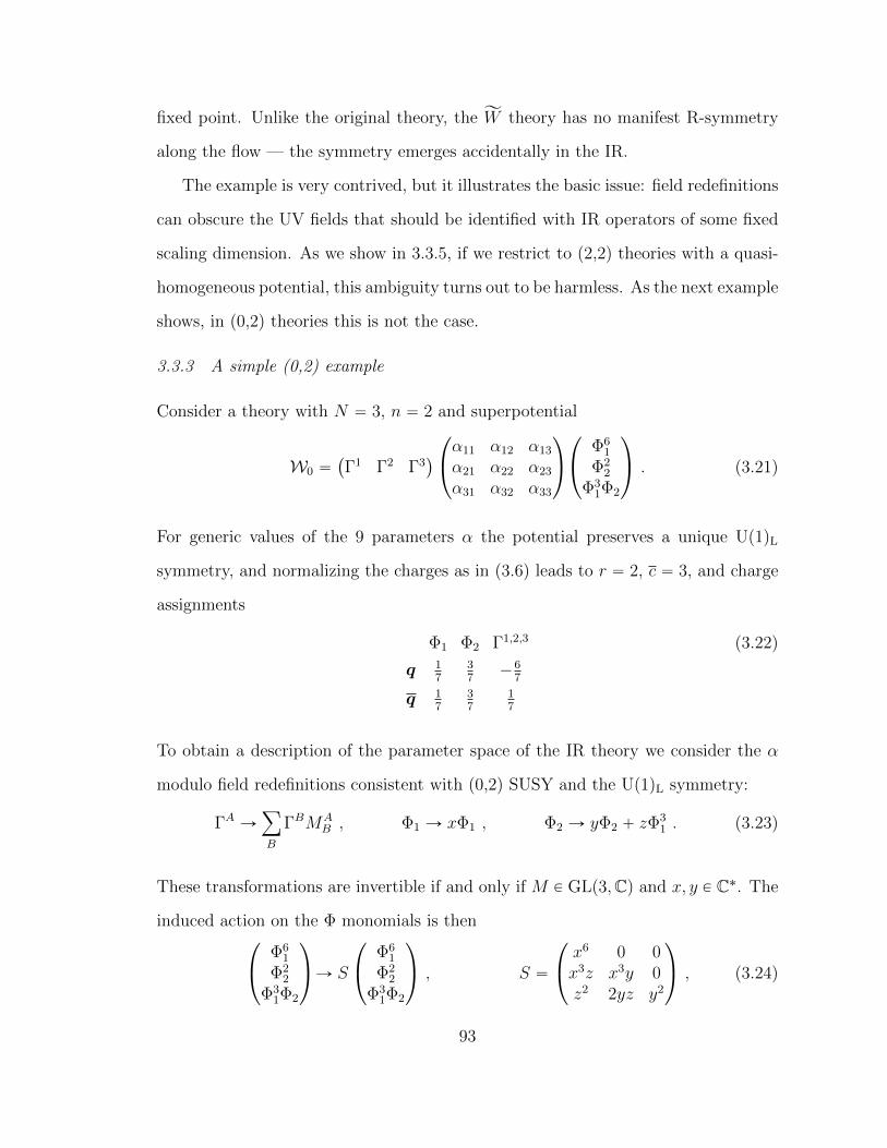
fixed point. Unlike the original theory, the ĂW theory has no manifest R-symmetry
along the flow — the symmetry emerges accidentally in the IR.
The example is very contrived, but it illustrates the basic issue: field redefinitions
can obscure the UV fields that should be identified with IR operators of some fixed
scaling dimension. As we show in 3.3.5, if we restrict to (2,2) theories with a quasi-
homogeneous potential, this ambiguity turns out to be harmless. As the next example
shows, in (0,2) theories this is not the case.
3.3.3 A simple (0,2) example
Consider a theory with N “ 3, n “ 2 and superpotential
W0 “`
Γ1 Γ2 Γ3˘
¨
˝
α11 α12 α13
α21 α22 α23
α31 α32 α33
˛
‚
¨
˝
Φ61
Φ22
Φ31Φ2
˛
‚ . (3.21)
For generic values of the 9 parameters α the potential preserves a unique Up1qL
symmetry, and normalizing the charges as in (3.6) leads to r “ 2, c “ 3, and charge
assignments
Φ1 Φ2 Γ1,2,3
q 17
37
´67
q 17
37
17
(3.22)
To obtain a description of the parameter space of the IR theory we consider the α
modulo field redefinitions consistent with (0,2) SUSY and the Up1qL symmetry:
ΓA Ñÿ
B
ΓBMAB , Φ1 Ñ xΦ1 , Φ2 Ñ yΦ2 ` zΦ3
1 . (3.23)
These transformations are invertible if and only if M P GLp3,Cq and x, y P C˚. The
induced action on the Φ monomials is then¨
˝
Φ61
Φ22
Φ31Φ2
˛
‚Ñ S
¨
˝
Φ61
Φ22
Φ31Φ2
˛
‚ , S “
¨
˝
x6 0 0x3z x3y 0z2 2yz y2
˛
‚ , (3.24)
93
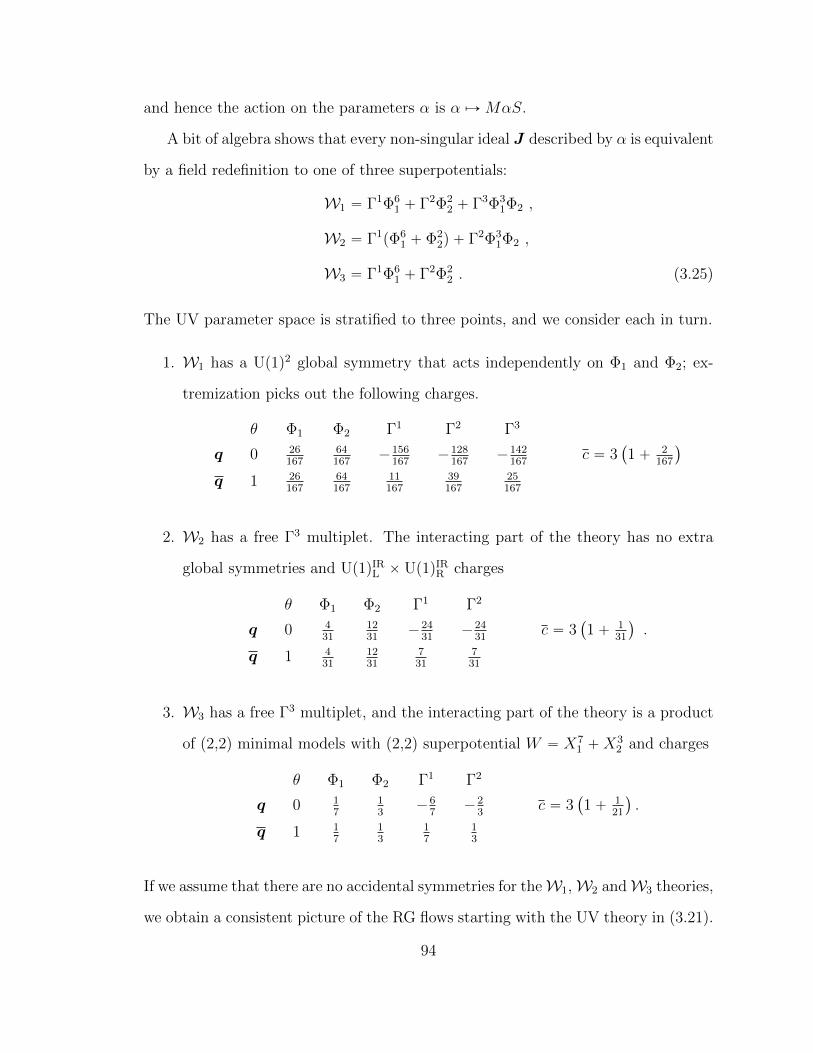
and hence the action on the parameters α is α ÞÑMαS.
A bit of algebra shows that every non-singular ideal J described by α is equivalent
by a field redefinition to one of three superpotentials:
W1 “ Γ1Φ61 ` Γ2Φ2
2 ` Γ3Φ31Φ2 ,
W2 “ Γ1pΦ6
1 ` Φ22q ` Γ2Φ3
1Φ2 ,
W3 “ Γ1Φ61 ` Γ2Φ2
2 . (3.25)
The UV parameter space is stratified to three points, and we consider each in turn.
1. W1 has a Up1q2 global symmetry that acts independently on Φ1 and Φ2; ex-
tremization picks out the following charges.
θ Φ1 Φ2 Γ1 Γ2 Γ3
q 0 26167
64167
´156167
´128167
´142167
c “ 3`
1` 2167
˘
q 1 26167
64167
11167
39167
25167
2. W2 has a free Γ3 multiplet. The interacting part of the theory has no extra
global symmetries and Up1qIRL ˆ Up1qIRR charges
θ Φ1 Φ2 Γ1 Γ2
q 0 431
1231
´2431
´2431
c “ 3`
1` 131
˘
.
q 1 431
1231
731
731
3. W3 has a free Γ3 multiplet, and the interacting part of the theory is a product
of (2,2) minimal models with (2,2) superpotential W “ X71 `X
32 and charges
θ Φ1 Φ2 Γ1 Γ2
q 0 17
13
´67
´23
c “ 3`
1` 121
˘
.
q 1 17
13
17
13
If we assume that there are no accidental symmetries for theW1,W2 andW3 theories,
we obtain a consistent picture of the RG flows starting with the UV theory in (3.21).
94
There are three basins of attraction; each has a central charge c ą 3, a set of charges
consistent with unitarity bounds and no marginal deformations. Moreover, we can
construct interpolating RG flows W3 ÑW2 ÑW1 by adding relevant deformations
to the superpotentials. However, W1 has no Up1qL-invariant relevant deformations
that make it flow to a putative c “ 3 theory described by W0.
We conclude that (0,2) LG RG flows have accidental symmetries, and identifying
these is key in order to correctly pinpoint even basic properties of the IR theory. For
instance, we see in the example at hand that no point in the UV parameter space
leads to an IR theory with c “ 3 and r “ 2.
3.3.4 Puzzles from enhanced symmetries
There are two questions that probably occur to our erudite reader. First, what’s the
big deal? One has to take account of field redefinitions when discussing the parameter
space of a theory, and it seems that all we learned here is that the parameter space
is smaller than one may have naively thought. Second, is it not perverse to discover
some accidental symmetries associated toW1,2,3 versusW0 but then blithely assume
that W1,2,3 do not themselves suffer from accidents?
There is a pragmatic answer to the second question: we assume there are no
accidents unless we are able to identify some paradox in the putative description of
the IR physics in terms of the UV parameters. In our example we find such a paradox:
while a generic W has a unique global symmetry in the UV, there are special points
with enhanced symmetries and a central charge that exceeds the putative c “ 3 of
the generic W ! Once we take into account the accidental symmetries, we discover
that the enhanced symmetries are unavoidable, and there is no c “ 3 theory that
can be reached within the parameter space of these UV theories. It is also easy to
construct paradoxical examples that would violate unitarity bounds unless one takes
accidents into account [79].
95
The answer to the first question is contained in this pragmatic perspective. The
“big deal” is that in the examples with which we are most familiar, namely the (2,2)
LG theories, one never encounters these enhanced symmetry puzzles: although there
are plenty of points with enhanced symmetries, these never mix with Up1qIRR , and
the central charge does not jump for any choice of non-singular (2,2) superpotential.
We discuss this in detail in the next section.
3.3.5 Enhanced symmetries of (2,2) LG theories
Consider a (2,2) LG theory with a quasi-homogeneous (2,2) superpotential W pXq
obeying W ptqiXiq “ tW pXq. Unless W satisfies an independent quasi-homogeneity
condition, the (2,2) R-symmetries are fixed uniquely, giving charge q “ qi to Φi and
Γi, where pΦi,Γiq are the (0,2) components of the (2,2) multiplet Xi. Without loss
of generality we can restrict attention to 0 ă qi ă 12.8 A special case occurs when
we can split the fields tXiu Ñ tXau Y tXpu so that W “ W 1pXaq `W 2pXpq. This
leads to an enhanced symmetry, but the enhancement is very large: on both the left
and right we obtain two N “ 2 superconformal algebras with c1 and c2 that add up
to the total c. The enhanced right-moving Up1q symmetry is not part of an N=2
Kac-Moody algebra: there are two commuting N=2 superconformal algebras, and
each Up1q is the lowest component of a different N “ 2 algebra. Thinking of this
theory as a (0,2) LG model and carrying out c-extremization leads to the same result
for c and charges of the chiral fields.
We will now show that in non-singular (2,2) theories this is the only way that
enhanced symmetries occur. Hence, there are no (2,2) accidents.
A necessary and sufficient condition to be able to perform the split tXiu Ñ
tXau Y tXpu and W “ W 1pXaq `W 2pXpq is that the matrix of second derivatives
8 We assume qi ą 0. In that case for a non-singular potential any fields with qi ě 12 can beeliminated by their equations of motion.
96
Wki is block diagonal in the two sets of variables. 9 Since we understand the symmetry
enhancement in that case, we assume that Wki has no non-trivial block.10 We will
now show that no additional symmetry is possible when W is non-singular. The
argument uses three facts.
1. A non-singular W can satisfy at most one linearly independent quasi-homogeneous
relation. To see this, suppose the contrary. By taking linear combinations of two
relations we arrive atř
i αiXiWi “ 0. We can now split the fields Xi according to
αi ą 0, αi ă 0, or αi “ 0: tXiu Ñ tYau Y tZsu Y tUαu and recast the relation as
ÿ
a
βaYaWa “ÿ
s
γsZsWs , (3.26)
where βa, γm ą 0. Without loss of generality we may assume β1 “ 1 ě βa for a ‰ 1.
Every monomial in W that contains Y1 must contain at least one Z. Hence, W will
be singular unless W Ą Y m1 Zs for some s, say s “ 1. Similarly, dW |Y“0 will be
independent of Z1 unless W Ą Zp1Ya for some a, which requires βa “ γ1p “ pm ą 1,
where the last inequality follows since W has no quadratic terms in the fields. That
is in contradiction with βa ď 1, so the theory must be singular.
2. Suppose we have a symmetry of the (2,2) theory that commutes with the (0,2)
SUSY algebra. This means that there are charges Q1i and q1i such that
´Q1iWi “ÿ
j
q1jXjWij ùñ ´Q1iWik “ q1kWki `ÿ
j
qjXjWjik .
Exchanging i and k in the second equation and taking the difference, we obtain
pQ1k ´ q1kqWki “ WkipQ
1i ´ q
1iq .
9 We use the shorthand Wi “ BW BXi, Wki “ BW BXkBXi , etc.
10 Take the n ˆ n matrix Wki and set to 1 all non-zero components. The result is a symmetricmatrix Aki that is the adjacency matrix for a graph G on n nodes, with each Aki ‰ 0 specifying apath in the graph from node k to node i. The statement that there is no non-trivial block is simplythat G is connected.
97
This means that whenever Wki ‰ 0 we need Q1k ´ q1k “ Q1i ´ q
1i.
11
3. The (2,2) superpotential satisfies
pq1i ´Q1iqW ´
ÿ
j
q1jXjWj “ U i ,
where U i is independent of X i. This follows by integrating the quasi-homogeneity
condition obeyed by Wi.
Using these observations, we now complete the argument as follows. Since Wki
does not contain a non-trivial block, we see from the second fact that for all k, i
Q1k ´ q1k “ Q1i ´ q1i. Combining this with the third fact, we find that W satisfies a
quasi-homogeneity relation W ptq1jXjq “ tq
1i´Q
1iW pXq; the first fact then implies that
either q1i “ cqi and q1i ´Q1i “ c, or W is singular.
3.3.6 Subtleties for heterotic vacua
We have seen that the identification of UV parameters with a deformation space of
an IR CFT, while reasonably well understood for (2,2) theories, is more subtle for
(0,2) theories. The difference is that while in non-singular (2,2) theories enhanced
symmetries are always associated to a decomposition of the UV theory into non-
interacting components, this is not the case for (0,2) models. An enhanced symmetry
of a (0,2) model does generically mix with the naive Up1qR, so that the enhanced
symmetry point has a different central charge from what one might expect naively.
As illustrated by the example in section 3.3.3, the RG fixed points of a (0,2) model
need not realize any CFT with the naive central charge.
There are situations where the consequences are more benign: there is a choice
of UV parameters that leads to a CFT with the expected IR symmetries, but even
then the identification of UV parameters with marginal deformations of the IR theory
requires a careful study of the field redefinition orbits on the space of UV parameters.
11 This is trivially satisfied for the usual (2,2) Up1qL, where Qi “ qi ´ 1.
98
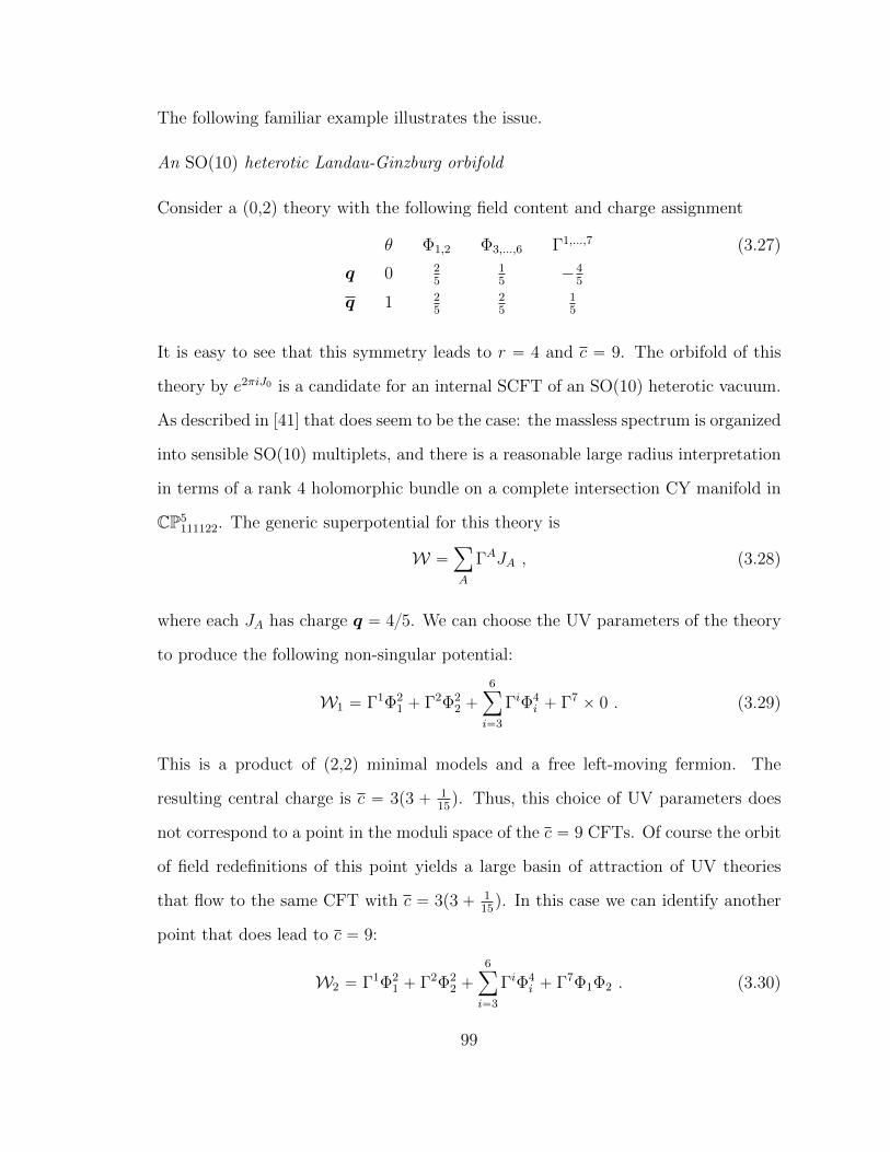
The following familiar example illustrates the issue.
An SOp10q heterotic Landau-Ginzburg orbifold
Consider a (0,2) theory with the following field content and charge assignment
θ Φ1,2 Φ3,...,6 Γ1,...,7
q 0 25
15
´45
q 1 25
25
15
(3.27)
It is easy to see that this symmetry leads to r “ 4 and c “ 9. The orbifold of this
theory by e2πiJ0 is a candidate for an internal SCFT of an SOp10q heterotic vacuum.
As described in [41] that does seem to be the case: the massless spectrum is organized
into sensible SOp10q multiplets, and there is a reasonable large radius interpretation
in terms of a rank 4 holomorphic bundle on a complete intersection CY manifold in
CP5111122. The generic superpotential for this theory is
W “ÿ
A
ΓAJA , (3.28)
where each JA has charge q “ 45. We can choose the UV parameters of the theory
to produce the following non-singular potential:
W1 “ Γ1Φ21 ` Γ2Φ2
2 `
6ÿ
i“3
ΓiΦ4i ` Γ7
ˆ 0 . (3.29)
This is a product of (2,2) minimal models and a free left-moving fermion. The
resulting central charge is c “ 3p3 ` 115q. Thus, this choice of UV parameters does
not correspond to a point in the moduli space of the c “ 9 CFTs. Of course the orbit
of field redefinitions of this point yields a large basin of attraction of UV theories
that flow to the same CFT with c “ 3p3` 115q. In this case we can identify another
point that does lead to c “ 9:
W2 “ Γ1Φ21 ` Γ2Φ2
2 `
6ÿ
i“3
ΓiΦ4i ` Γ7Φ1Φ2 . (3.30)
99
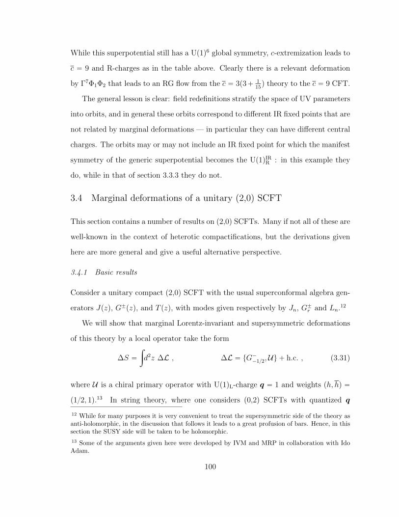
While this superpotential still has a Up1q6 global symmetry, c-extremization leads to
c “ 9 and R-charges as in the table above. Clearly there is a relevant deformation
by Γ7Φ1Φ2 that leads to an RG flow from the c “ 3p3` 115q theory to the c “ 9 CFT.
The general lesson is clear: field redefinitions stratify the space of UV parameters
into orbits, and in general these orbits correspond to different IR fixed points that are
not related by marginal deformations — in particular they can have different central
charges. The orbits may or may not include an IR fixed point for which the manifest
symmetry of the generic superpotential becomes the Up1qIRR : in this example they
do, while in that of section 3.3.3 they do not.
3.4 Marginal deformations of a unitary (2,0) SCFT
This section contains a number of results on (2,0) SCFTs. Many if not all of these are
well-known in the context of heterotic compactifications, but the derivations given
here are more general and give a useful alternative perspective.
3.4.1 Basic results
Consider a unitary compact (2,0) SCFT with the usual superconformal algebra gen-
erators Jpzq, G˘pzq, and T pzq, with modes given respectively by Jn, G˘r and Ln.12
We will show that marginal Lorentz-invariant and supersymmetric deformations
of this theory by a local operator take the form
∆S “
ż
d2z ∆L , ∆L “ tG´´12,Uu ` h.c. , (3.31)
where U is a chiral primary operator with Up1qL-charge q “ 1 and weights ph, hq “
p12, 1q.13 In string theory, where one considers (0,2) SCFTs with quantized q
12 While for many purposes it is very convenient to treat the supersymmetric side of the theory asanti-holomorphic, in the discussion that follows it leads to a great profusion of bars. Hence, in thissection the SUSY side will be taken to be holomorphic.
13 Some of the arguments given here were developed by IVM and MRP in collaboration with IdoAdam.
100
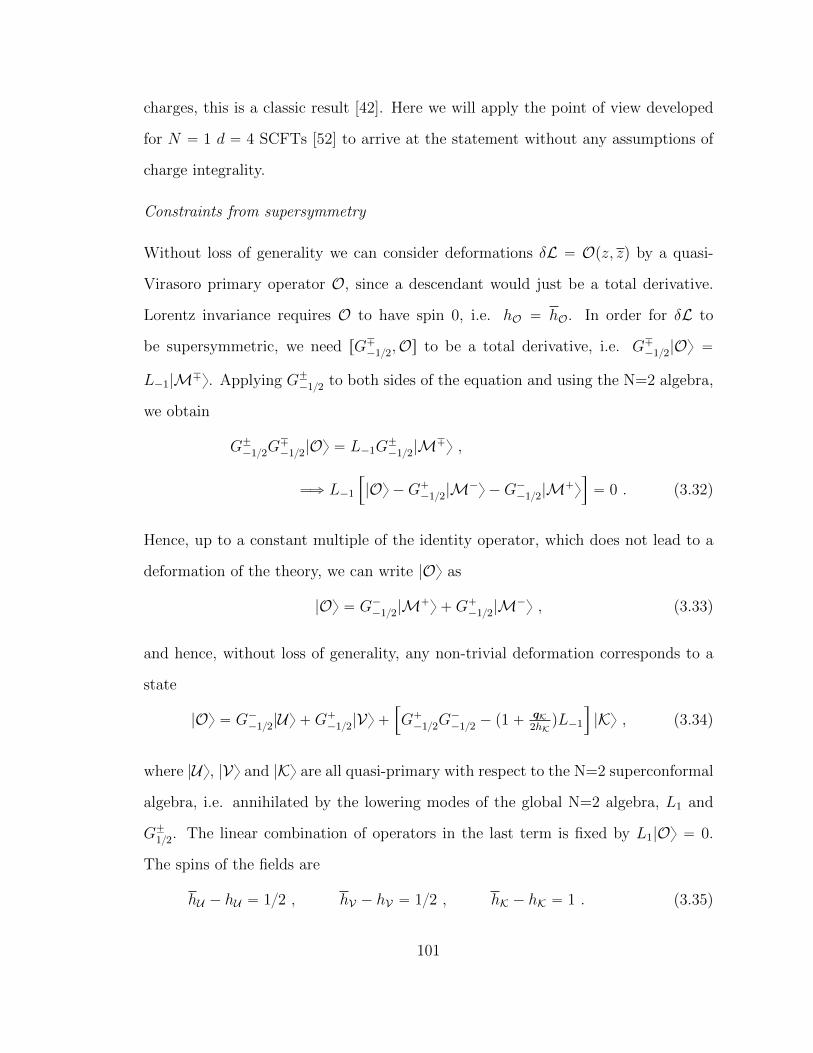
charges, this is a classic result [42]. Here we will apply the point of view developed
for N “ 1 d “ 4 SCFTs [52] to arrive at the statement without any assumptions of
charge integrality.
Constraints from supersymmetry
Without loss of generality we can consider deformations δL “ Opz, zq by a quasi-
Virasoro primary operator O, since a descendant would just be a total derivative.
Lorentz invariance requires O to have spin 0, i.e. hO “ hO. In order for δL to
be supersymmetric, we need rG¯´12,Os to be a total derivative, i.e. G¯
´12|Oy “
L´1|M¯y. Applying G˘´12 to both sides of the equation and using the N=2 algebra,
we obtain
G˘´12G
¯
´12|Oy “ L´1G˘
´12|M¯y ,
ùñ L´1
”
|Oy ´G`´12|M
´y ´G´
´12|M`y
ı
“ 0 . (3.32)
Hence, up to a constant multiple of the identity operator, which does not lead to a
deformation of the theory, we can write |Oy as
|Oy “ G´´12|M
`y `G`
´12|M´y , (3.33)
and hence, without loss of generality, any non-trivial deformation corresponds to a
state
|Oy “ G´´12|Uy `G
`
´12|Vy `”
G`´12G
´
´12 ´ p1`qK2hKqL´1
ı
|Ky , (3.34)
where |Uy, |Vy and |Ky are all quasi-primary with respect to the N=2 superconformal
algebra, i.e. annihilated by the lowering modes of the global N=2 algebra, L1 and
G˘12. The linear combination of operators in the last term is fixed by L1|Oy “ 0.
The spins of the fields are
hU ´ hU “ 12 , hV ´ hV “ 12 , hK ´ hK “ 1 . (3.35)
101
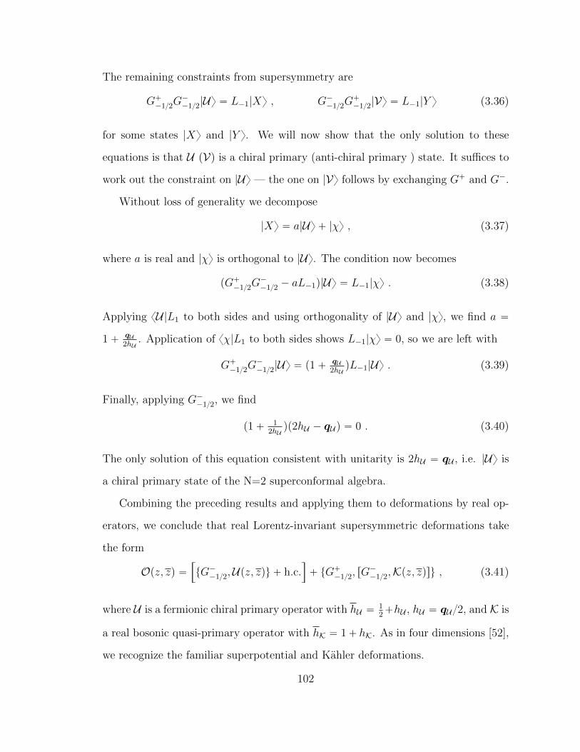
The remaining constraints from supersymmetry are
G`´12G
´
´12|Uy “ L´1|Xy , G´´12G
`
´12|Vy “ L´1|Y y (3.36)
for some states |Xy and |Y y. We will now show that the only solution to these
equations is that U (V) is a chiral primary (anti-chiral primary ) state. It suffices to
work out the constraint on |Uy — the one on |Vy follows by exchanging G` and G´.
Without loss of generality we decompose
|Xy “ a|Uy ` |χy , (3.37)
where a is real and |χy is orthogonal to |Uy. The condition now becomes
pG`´12G
´
´12 ´ aL´1q|Uy “ L´1|χy . (3.38)
Applying xU |L1 to both sides and using orthogonality of |Uy and |χy, we find a “
1` qU2hU
. Application of xχ|L1 to both sides shows L´1|χy “ 0, so we are left with
G`´12G
´
´12|Uy “ p1`qU2hUqL´1|Uy . (3.39)
Finally, applying G´´12, we find
p1` 12hUqp2hU ´ qUq “ 0 . (3.40)
The only solution of this equation consistent with unitarity is 2hU “ qU , i.e. |Uy is
a chiral primary state of the N=2 superconformal algebra.
Combining the preceding results and applying them to deformations by real op-
erators, we conclude that real Lorentz-invariant supersymmetric deformations take
the form
Opz, zq “”
tG´´12,Upz, zqu ` h.c.
ı
` tG`´12, rG
´
´12,Kpz, zqsu , (3.41)
where U is a fermionic chiral primary operator with hU “12`hU , hU “ qU2, and K is
a real bosonic quasi-primary operator with hK “ 1` hK. As in four dimensions [52],
we recognize the familiar superpotential and Kahler deformations.
102
Marginal operators
If we impose in addition that the perturbation is marginal, we obtain the constraints
qU “ 1 and hK “ 0. The latter implies that L´1|Ky “ 0, i.e. Kpzq is an anti-
holomorphic conserved current that leads to a trivial deformation of the action. We
arrive at the result (3.31).
3.4.2 A few consequences
The preceding analysis, when combined with some basic assumptions about super-
conformal perturbation theory, leads to important constraints on (2,0) SCFTs. The
key feature is that we can use a (2,0) superspace to recast the marginal deformations
into the form
∆S “
ż
d2z
ż
dθ αiUi ` h.c. , (3.42)
where αi denote the couplings and Ui are denote the chiral primary marginal fermi su-
perfields. Assuming there exists a manifestly supersymmetric regularization scheme
for conformal perturbation theory, the renormalized action at a renormalization scale
µ must take the form
∆Lren “
ż
d2θ
«
Zapα, α;µqJa `
ÿ
A
µ2´dAKA
ff
`
"ż
dθ“
pαi ` δαipα;µqqUi ` ζIpα;µqUI
‰
` h.c.
*
. (3.43)
At the conformal point (α “ 0) the Ja and KA are real operators of dimension
∆a “ 2 and ∆A ą 2, while the Ui and UI are chiral primary operators with q “ 1
and q ą 1 respectively.14 The first line is parallels the N “ 1 d “ 4 situation;
however, the second line is new, following from the fact that the UiUj OPE will in
14 Compactness of the CFT ensures a gap in dimensions between Ja and KA, as well as betweenUi and UI .
103
general have singular z dependence. Of course supersymmetry still requires that the
renormalization of the superpotential should be holomorphic in the parameters.
Marginal irrelevance
Marginal deformations preserve the R-symmetry of the original SCFT. Hence, the
unitarity bound hU ě q2 implies that a marginal deformation is at worst marginally
irrelevant and never marginally relevant.
D-terms and F-terms
Assuming that conformal perturbation theory is renormalizable, the terms involving
the KA and UI do not arise, and scale invariance of the theory is equivalent to
Dapα, αq ” µ
B
BµZa“ 0 and F
ipαq ” µ
B
Bµδαi “ 0. (3.44)
A two-dimensional unitary compact scale-invariant theory is automatically confor-
mal [87], so every deformation satisfying these “D-term” and “F-term” constraints
is exactly marginal.
The “D-term” obstructions to marginality are exactly the same as in the d “ 4
case studied in [52] — such a scale dependence requires the breaking of a global
right-moving symmetry. This is easy to understand at leading order in conformal
perturbation theory. In the presence of abelian currents Ja, the OPE of U with its
conjugate takes the form
Uipz, zqU pw,wq „gi
pz ´ wqpz ´ wq2`
giqiaJ
apw,wq
pz ´ wqpz ´ wq` . . . , (3.45)
where Ja“ γabJ b, and zzxJapzqJ bp0qy “ γab in the undeformed theory. This leads
to a logarithmic divergence in conformal perturbation theory proportional to
ż
d2wG`´12G
´
´12
ż
d2z|αi|2qiaJ
apw,wq
pz ´ wqpz ´ wq„ log µˆ |αi|2qiaJ
apw,wq , (3.46)
104
which corresponds to the leading order D-term proportional to
Da “ÿ
i
|αi|2qia . (3.47)
In applications to heterotic compactifications such a symmetry necessarily corre-
sponds to a gauge boson in the space-time theory, and the space-time picture of the
breaking is just the Higgs mechanism: the obstruction to marginality of a coupling
α that breaks a right-moving symmetry is encoded in a space-time D-term potential.
We believe that in (0,2) LG models without an orbifold there are no F-term
obstructions. The reason is simple: the free field UV presentation of the theory
comes with the usual non-renormalization theorems for the superpotential, so the
only divergences we expect to encounter will correspond to D-term counter-terms.
The two sources of obstruction are in one to one correspondence with the two
ways in which a short chiral primary multiplet can combine into a long multiplet
of (2,0) SUSY. Suppose we consider an infinitesimal (2,0) SUSY deformation under
which a marginal chiral primary state |Uy acquires weights ph, hq “ p12` ε
2, 1 ` ε
2q.
In this case |Uy is no longer chiral primary, and by a choice of basis we can consider
two separate cases:
G`´12|Uy ‰ 0 , G´12|Uy “ 0 , or G`
´12|Uy “ 0 , G´12|Uy ‰ 0 . (3.48)
In other words, |Uy remains primary but is no longer chiral, or it remains chiral but
fails to be primary. The first case corresponds to an F-term obstruction, where at
ε “ 0 we have two chiral primary superfields pU ,Fq with qU “ 1 and qF “ 2 and
h “ 1, while for ε ą 0 we find a complex long multiplet with lowest component |Uy
and G`´12|Uy “
?ε|Fy.15 The second case corresponds to a D-term obstruction,
where at ε “ 0 we have chiral primary superfields U , its anti-chiral conjugate U ,
15 In a c “ 9 theory with spectral flow there is a canonical F for every U in the theory. Indeed, asobserved in [12, 36, 42], the F (2,0) superfields can be used to construct vertex operators for thespace-time auxiliary fields residing in chiral multiplets of the associated four-dimensional theory.
105
and a Kac-Moody current J ; for ε ą 0 we obtain a long real multiplet with lowest
component J and descendants G`´12|Jy “
?ε|Uy and G´
´12|Jy “?ε|Uy.
In particular, we see that there are no F-term obstructions if the undeformed
theory has no chiral primary operators with q “ 2 and h “ 1. This is the case, for
instance, in every (2,0) SCFT with c ă 6. If there are also no left-moving Kac-Moody
symmetries then every (2,0) marginal deformation must remain exactly marginal. In
appendix B.1 we mention a simple example illustrating an F-term obstruction at
c “ 9.
Kahler geometry of the moduli space
One can use the same reasoning as in [52] to argue that the space of truly marginal
deformations of a (2,0) SCFT must be a Kahler manifold. This is because the D-term
constraints and the quotient by global symmetries lead to a toric quotient on the
space of marginal couplings, while the F-term constraints are manifestly holomorphic
constraints, restricting the truly marginal directions to a Kahler subvariety of the
toric variety. In heterotic compactification this can of course be argued either from
the space-time heterotic supergravity or by using additional assumptions of a (2,0)
SCFT with integral charges [86]. The argument given here is more direct and general.
Application to (2,2) theories
The case of a (2,2) SCFT and its (2,2)-preserving deformations is much simpler.
There are two types of superpotential deformations: the chiral and the twisted chiral.
The former corresponds to deformations by chiral primary (c,c) ring operators, while
the latter by the (a,c) ring operators. Supersymmetry implies that twisted chiral
parameters can never show up in the renormalized chiral superpotential and vice-
versa. Moreover, the OPE of the (c,c) and (a,c) chiral primaries with themselves is
non-singular, so that neither potential is corrected—there are no F-term obstructions
106
to marginality. Hence, all marginal (c,c) and (a,c) symmetry-preserving deformations
are truly marginal. This is again a familiar story in string applications [35, 42] .
Accidents beyond field redefinitions
We can now see that the field redefinitions of (0,2) LG theories do not describe all
accidents. It is not the case that every direction transverse to field redefinition orbits
corresponds to a marginal deformation of the IR theory. This is due to the possibility
that marginal deformations of a (0,2) theory can turn out to be marginally irrelevant.
In (0,2) LG theories this is due to D-term obstructions where a Up1q symmetry is
broken by turning on operators with a definite sign of the Up1q charge. We give an
example of this phenomenon in a well-known heterotic vacuum in appendix B.2.
3.4.3 Deformations and left-moving abelian currents
As a final application of the preceding results, we consider the interplay between
deformations of a (2,0) SCFT and left-moving currents.
A (2,0) SCFT may possess a KM algebra on the SUSY side of the world-sheet
in addition to the Up1qL current JL in the N “ 2 multiplet. Such structures are
familiar from heterotic compactifications preserving 8 space-time supercharges in four
dimensions — when realized geometrically these correspond to geometries π : X Ñ
K3 — principal T 2 fibrations over a base K3 [20, 82]. In each such case we can use
a Sugawara-like decomposition to decompose the N “ 2 world-sheet superconformal
algebra (SCA) into two commuting sets of generators, one associated to the KM
algebra, and the other corresponding to the remaining degrees of freedom.
Suppose we have an abelian current algebra Up1q with current J1. There are two
ways that the decomposition can work. If J does not belong to a multiplet of the
Ac SCA, then we must have a decomposition
Ac “ A1c1 ‘A2c2 , (3.49)
107
where c “ c1 ` c2, and the lowest components of the N=2 multiplets of A1 and A2
are obtained by appropriate linear combinations of JL and J1. We are familiar with
such examples from above: this happens whenever the LG theory decomposes into
a product of two non-interacting theories.
If J does belong to a multiplet of A, then it must be accompanied by a second
Up1q Kac-Moody current J2, as well as weight h “ 12 operators ψ1 and ψ2. Together
these arrange themselves into a well-known c “ 3 unitary representation of N “ 2:
JL “: ψψ : , G` “?
2ψ , G´ “?
2ψ , T “: : ´12p: ψBψ : ` : ψBψ :q ,
(3.50)
where ψ and have the free-field OPEs
ψpzqψpwq „ pz ´ wq´1, pzqpwq „ pz ´ wq´2. (3.51)
This is equivalent to the holomorphic sector of a T 2 (1,0) non-linear sigma model,
and we will call it Afree3 .
There is a key difference between these two generalizations. In the first case,
there are generally deformations that can break the extra left-moving symmetry —
in (2,2) LG this happens when we move away from a Gepner point to a more generic
theory. In the second case such breaking is impossible. To see this, we just need
to apply what we learned about the structure of SUSY deformations in conformal
perturbation theory. Since our algebra splits as
Ac “ A1c´3 ‘Afree3 , (3.52)
a marginal deformation has a similar decomposition
U “ U 1 ` Sψ , (3.53)
where U 1 is a chiral primary operator with h “ 1 and q1 “ 1, while S is a (0,1)
current. The deformation of the action is then
G´´12 ¨ U “ G1´
´12 ¨ U1`?
2S . (3.54)
This is neutral with respect to JL, and . More generally, any relevant deformation
must be of the form U “ U 1 with q1 ă 1.
108
3.5 Toric geometry of the deformation space
In the previous sections we saw that accidental symmetries play an important role in
(0,2) Landau-Ginzburg theories, and more generally, in (0,2) SCFTs. In this section
we will describe a conjecture that allows us to account for these accidents in a certain
class of (0,2) LG theories. In that context our goal is to describe the moduli space
M of IR fixed points corresponding to a class of UV data determined by a choice of
charges qi and QA which have the expected central charge
c “ 3pn´N ` rq , r “ ´ÿ
A
QA ´ÿ
i
qi . (3.55)
To do so, we need to perform two steps:
1. decompose the UV parameter space into orbits under the action of field redef-
initions;
2. determine which orbits contribute to M.
The result is expected to be a (typically singular) Kahler space. In general these
are rather formidable tasks. The group of field redefinitions is rather large and
the space of orbits is non-separable. A reasonable geometry can only emerge after
implementing the second task. This involves excluding two types of orbits:
• Along a discriminant locus ∆ in parameter space, the superpotential is singular.
The discriminant will clearly be invariant under field redefinitions, and orbits
contained in ∆ will not contribute to M.
• For some non-singular values of the parameters, the theory will have accidental
symmetries in the IR. As we have seen, in some cases these symmetries will
mix nontrivially with the R-symmetry and the central charge of the IR fixed
point will be larger than c. Thus, these orbits as well need to be excluded from
M.
109
In general, the second step is difficult even if one restricts attention to symmetries
which act diagonally on the UV fields. Detecting the basin of attraction of some
component of the IR moduli space with central charge c1 ą c requires a determination
of the R-symmetry along each such component to find which deformations away from
this locus are in fact irrelevant.
3.5.1 The toric conjecture
There is a simpler version of both of these problems that may be tractable. The
group of field redefinitions always contains an abelian subgroup, the complexification
of the Up1qnˆUp1qN subgroup of the global symmetry of the free kinetic terms, that
corresponds to rescaling the chiral fields of the theory. In particular, if we write the
most general superpotential in our class as
W “ÿ
A
ΓAÿ
mP∆A
αAmź
i
Φmii , (3.56)
where
∆A “ tm P Zn |ř
imiqi “ ´QAu (3.57)
describes the lattice points in the Newton polytope for JA, then the field redefinitions
Φi ÞÑ tiΦi , ΓA ÞÑ τAΓA (3.58)
lead to a TC “ pC˚qN´n`1 action16 on the space of UV parameters Y “ Cř
A |∆A|
αAm ÞÑ τAś
i tmii ˆ αAm . (3.59)
We will refer to these as toric field redefinitions.
We now restrict attention to these toric actions in both of the tasks listed above.
Namely, we decompose the parameter space into TC orbits and exclude those orbits
that either lie in ∆ or exhibit accidental symmetries contained in TC and lead to
16 The rank of the C˚ action is reduced by 1 due to the quasi-homogeneity of W.
110
c1 ą c. The result, which we will call MT , will in some cases be equivalent to M,
but in general the two will differ. We will comment on this further below.
The action of the compact torus T Ă TC , given by restricting to |t| “ |τ | “ 1 ,
determines a moment map µ “ pλ; Λq : Y Ñ RN`n with
λi “ÿ
A
ÿ
mP∆A
mi|αAm|2 , ΛA “
ÿ
mP∆A
|αAm|2 . (3.60)
Quasi-homogeneity of W implies that the image lies in the hyperplaneÿ
i
qiλi `ÿ
A
QAΛA “ 0 . (3.61)
The image of µ is the intersection of this hyperplane with a cone, determined by the
charges, inside the positive orthant in RN`n. This intersection is itself a cone pΣ, of
dimension N ` n ´ 1. The level sets of µ determine a selection of orbits: generic
orbits will be N ` n ´ 1 dimensional, but the action will degenerate along points
with a non-trivial stabilizer subgroup, leading to orbits of smaller dimension.17 More
precisely, the cone pΣ can be subdivided into a fan Σ, such that the collection of orbits
containing a point for which µpαq “ µ˚ is determined by the cone of Σ that contains
µ˚. This is the secondary fan for the T action. We now have enough structure to
state our conjecture.
Conjecture
The toric moduli space MT is the complement of the discriminant subvariety ∆ in
a toric variety
V “ µ´1pλ˚,Λ˚qT , (3.62)
where
λ˚i “ 1´ qi , Λ˚A “ 1`QA . (3.63)
17 There are orbifold singularities when the subgroup is discrete; we will focus on continuousstabilizer subgroups.
111
This is a rather strong statement, and we will not provide a complete proof but
rather some evidence for it. Some ideas on a possible derivation are discussed in sec-
tion 3.5.4. We will motivate the conjecture by combining our results and observations
from above with some facts about toric varieties.
We should note a few important points. First, V may turn out to be empty.
Second, while we claim that V z∆ describes MT as a variety, we do not make any
statement about the relation between the Zamolodchikov metric on the space of
marginal couplings and the metric on V obtained by the Kahler quotient. Finally,
in this chapter we will be concerned with orbits of continuous field redefinitions. In
general there will be additional discrete quotients that identify points in MT .
Combinatorics of the secondary fan
Codimension-one cones in Σ are associated with orbits containing a point at which a
single C˚ Ă TC is unbroken. More precisely, Gpq1,Q1q “ C˚ Ă TC acting with charges
q1i, Q1A on the chiral superfields will fix points at which
|αAm|2pQ1A `
ř
imiq1iq “ 0 for all A, m P ∆A . (3.64)
The µ-image of the TC orbits of such points will lie in a cone σpq1,Q1q generated by the
charge vectors of the αAm fixed by Gpq1,Q1q. Thus, the codimension-one cones of Σ are
determined by one-dimensional subgroups for which σpq1,Q1q has dimension N `n´ 2
and lies in the hyperplaneÿ
A
Q1AΛA `ÿ
i
q1iλi “ 0 . (3.65)
In terms of W the codimension-one cones of Σ correspond to subgroups for which
we can write a (possibly singular) family of models fixed precisely by pC˚q2. Cones
of higher codimension in the fan are boundaries of these cones and arise at the
intersections of these hyperplanes.18 Points in the interior of some cone of the fan (of
18 Note that this does not imply that cones of higher codimension correspond to models with largerunbroken symmetry: values of µ at the intersection of two codimension-one cones can be in the
112
any codimension) lie in the image of a collection of orbits determined by that cone.
Our conjecture is thus equivalent to the statement that the µ-image of the TC orbits
of models with central charge c intersects the cone σ˚ containing µ˚ in its interior.
A cone σ P Σ can be specified by its relation to the codimension-one cones σpq1,Q1q.
For each of these, σ either lies inside σpq1,Q1q, in which case µ P σ satisfy (3.65), or it
lies on one side or the other, meaning (3.65) is satisfied as a strict inequality for all
µ P σ. To prove our claim we thus need to show that orbits of points in parameter
space corresponding to models with central charge c are precisely those containing
in their image points satisfying the inequalities satisfied by µ˚. To do this we must
consider all codimension-one cones of Σ. We classify these by the nature of the
models exhibiting the enhanced symmetry.
3.5.2 Enhanced toric symmetries
Symmetries realized by a non-singular potential
Consider first the case of one-parameter subgroups of TC for which the generic point in
the locus they fix corresponds to a nonsingular model with a Up1q2 global symmetry.
The IR R-symmetry can then be determined by c-extremization as
qi “ tqi ` sq1i , QA “ tQA ` sQ
1A , (3.66)
where
L
ˆ
t´ 1s
˙
“
ˆ
0ř
i q1iλ˚i `
ř
AQ1AΛ˚A
˙
. (3.67)
L is the negative-definite 2ˆ 2 matrix defined in (3.11) and pq,Qq are normalized as
in (3.6). We now distinguish two situations.
1. c1 “ c. Ifÿ
i
q1iλ˚i `
ÿ
A
Q1AΛ˚A “ 0 , (3.68)
image of two distinct TC orbits, each of which is fixed by a different subgroup.
113
then the IR symmetry is given by pq;Qq, and the TC orbit of the model with enhanced
symmetry is a point in V . In this case, we can apply conformal perturbation theory
to deformations of this theory. The symmetry-breaking couplings αAm (those van-
ishing on the locus exhibiting enhanced symmetry) parameterize classically marginal
deformations away from the symmetric theory. The analysis of section 4 shows that
in fact some of these will be marginally irrelevant, and the moduli space is given to
first order in the symmetry-breaking couplings by the vanishing of the D-term for
the broken symmetry. We can write this explicitly here as
D “ÿ
A,nP∆A
pQ1A `ÿ
i
miq1iq|αAm|
2
“ÿ
i
q1iλi `ÿ
A
Q1AΛA . (3.69)
This holds at leading order in conformal perturbation theory about the symmetric
point, and our conjecture amounts here to the statement that higher order correc-
tions do not qualitatively modify the structure of the symplectic quotient that leads
to the variety V : while the metric may be modified, which orbits are kept and which
are excluded is not changed by higher order corrections. This implies that points in
V are TC orbits containing points whose image under µ lies in the cone σpq1,Q1q. We
see from (3.68) that this condition is satisfied by µ˚.
2. c1 ą c. If (3.68) is not satisfied, the central charge c1 determined by extremization
will be larger than c, and the TC orbit of the model with enhanced symmetry is not
a point of V . Moreover, the symmetry-breaking parameters αAm are not marginal
couplings in this theory. Solving (3.67) we find
s “ ´r
detL
˜
ÿ
i
q1iλ˚i `
ÿ
A
Q1AΛ˚A
¸
. (3.70)
Without loss of generality we can choose the sign of pq1, Q1q so that s is negative. Since
114
by construction all our couplings are invariant under pq;Qq, and by assumption L is
negative definite, the sign of the charge under the IR R-symmetry is then the opposite
of the charge under pq1, Q1q. Thus, couplings αAm for which Q1A`ř
imiq1i ą 0 will be
relevant deformations of the model with enhanced symmetry, while couplings with
the opposite charge will be irrelevant; couplings preserving the enhanced symmetry
are marginal. The TC orbits of points in parameter space corresponding to irrelevant
deformations of the symmetric model will not be points in V : as discussed above
they will exhibit an accidental symmetry in the IR and a central charge c1. Orbits
for which at least one relevant coupling is nonzero are characterized precisely by the
fact that they contain points for which the moment map satisfies
ÿ
i
q1iλi `ÿ
A
Q1AΛA ą 0 . (3.71)
This specifies one side of the hyperplane associated to the enhanced symmetry, and,
as we have shown, this is the side on which the point µ˚ lies.
Symmetries without a smooth realization
If every enhanced symmetry were realized by a non-singular W the discussion above
would suffice. In general, however, there are codimension-one cones in Σ associated
to one-parameter subgroups of TC for which it is not possible to construct a non-
singularW exhibiting the symmetry. In these cases the RG trajectories exhibiting the
enhanced symmetry along the flow are singular, and we cannot use their properties
to determine the local structure of the moduli space.
A simple example of this is given by the symmetry acting as ΓA Ñ τΓA for some
A with all the other fields invariant. This fixes the locus JA “ 0 which will in general
be singular (it will always be singular when n “ N). In this case, the corresponding
hyperplane is ΛA “ 0, and the associated codimension-one cone lies on the boundary
of pΣ.
115
More interesting is the case of a codimension-one cone in the interior of pΣ to
which the methods of the previous section do not apply. Our conjecture here is that
whenever the enhanced symmetry does not satisfy (3.68), non-singular models will
only exist when at least one symmetry-breaking coupling whose charge under the
broken symmetry is in accord with the sense of the inequality is non-zero. In parallel
with the second discussion in the previous subsection, TC orbits associated to points
in V will be those containing points whose image under µ lies on the side of the
hyperplane which contains the point µ˚.
There will also be codimension-one cones in Σ associated to one-parameter sub-
groups for which there is no non-singular model exhibiting the symmetry, but which
satisfy (3.68). Here as well we can classify the symmetry-breaking couplings by their
charge under the broken symmetry. In this case, we conjecture that non-singular
models will have nonzero values for at least one coupling of each sign. Restricting
to models with non-zero couplings of only one sign (as well as the neutral couplings)
will produce a singular model. The space of TC orbits associated to points in V
in this case will not be toric. It can, however, be described as the complement of
the symmetric locus (a component of ∆) in a (singular) toric variety. This contains
orbits containing points whose image under µ lies in the cone σpq1,Q1q. When we ex-
clude the singular symmetric locus here, we find precisely orbits that have nonzero
symmetry-breaking couplings with both signs of the broken charge. The point µ˚
clearly lies in this hyperplane.
3.5.3 Examples
A few examples may be helpful at this point. We proceed from a simple example
for which our methods produce correctly the actual moduli space to models demon-
strating their limitations.
116
A plain model
Consider first the class of models with n “ N “ 2 and charges
Φ1 Φ2 Γ1 Γ2
q 14
16´3
4´5
6
(3.72)
and c3 “ r “ 1` 16. The most general superpotential is
W “ Γ1`
α11φ31 ` α12φ1φ
32
˘
` Γ2`
α21φ52 ` α22φ
21φ
22
˘
, (3.73)
and the discriminant is
∆ “ α11α21 pα11α21 ´ α12α22q . (3.74)
This is an example of what we call a plain model: the torus TC includes all field
redefinitions consistent with the symmetry, so our toric considerations will in fact
generate the moduli space M itself.
The torus T “ Up1q3 action on C4 is characterized by the charges and moment
map components
D α11 α12 α21 α22
λ1 3 1 0 2
λ2 0 3 5 2
Λ1 1 1 0 0
Λ2 0 0 1 1
(3.75)
where the latter satisfy
3λ1 ` 2λ2 “ 9Λ1 ` 10Λ2 . (3.76)
There are six codimension-one cones in Σ. Only two of these are realized by non-
singular models; the remaining four comprise the boundaries of pΣ given by Λ1 ą
0 and Λ2 ą 0, as well as λ2 ´ 2Λ2 ą 0 and λ1 ´ Λ1 ą 0.
117
There are two codimension-one cones in the interior of pΣ. Consider first the
symmetry pq1;Q1q “ p1, 0;´3, 0q, which satisfies (3.68). The non-singular models
realizing this symmetry have α12 “ α22 “ 0. In fact the model reduces to a product
of two (2,2) minimal models and, as expected, the central charge is c. The symmetry
determined by pq1, Q1q “ p´1, 1;´2, 0q, for whichř
i q1iλ˚i `
ř
AQ1AΛ˚A ă 0, fixes mod-
els with α11 “ α22 “ 0.19 Under the broken symmetry, α11 is negatively charged and
α22 positively charged. We see from (3.74) that, in accordance with the conjecture,
non-singular models require a non-zero value for the negatively charged coupling.
The moduli spaceM is thus determined. We can fix two of the generators of TC
by setting α11 “ α21 “ 1, and the remaining couplings parameterize the toric variety
V “ C with invariant coordinate z “ α12α22. The moduli space is M “ V zr∆ where
the discriminant reduces in these coordinates to 1´ z.
A non-plain model
We can also consider the model with n “ N “ 2 and charges given by
Φ1 Φ2 Γ1 Γ2
q 46471
115471
´460471
´230471
(3.77)
with c3 “ r “ 1 ` 58471
. The most general superpotential invariant under this
symmetry is
W “ Γ1pα11Φ10
1 ` α12Φ51Φ2
2 ` α13Φ42q ` Γ2
pα21Φ51 ` α22Φ2
2q , (3.78)
and the discriminant is
∆ “ α11α222 ´ α12α21α22 ` α13α
221 . (3.79)
The torus T “ Up1q3 action on C5 is characterized by the charges and moment
19 Note that this symmetry leads a 2 ˆ 2 L matrix that is not negative-definite; however, thecorresponding superpotential is singular.
118
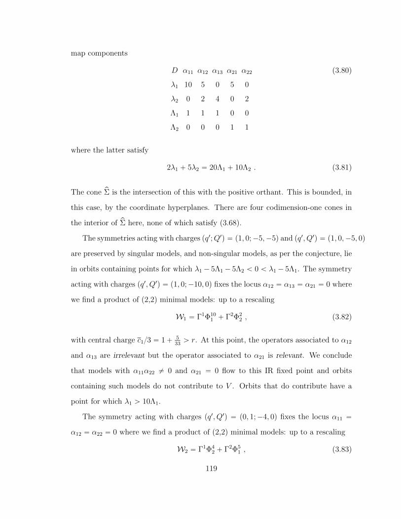
map components
D α11 α12 α13 α21 α22
λ1 10 5 0 5 0
λ2 0 2 4 0 2
Λ1 1 1 1 0 0
Λ2 0 0 0 1 1
(3.80)
where the latter satisfy
2λ1 ` 5λ2 “ 20Λ1 ` 10Λ2 . (3.81)
The cone pΣ is the intersection of this with the positive orthant. This is bounded, in
this case, by the coordinate hyperplanes. There are four codimension-one cones in
the interior of pΣ here, none of which satisfy (3.68).
The symmetries acting with charges pq1;Q1q “ p1, 0;´5,´5q and pq1, Q1q “ p1, 0,´5, 0q
are preserved by singular models, and non-singular models, as per the conjecture, lie
in orbits containing points for which λ1´ 5Λ1´ 5Λ2 ă 0 ă λ1´ 5Λ1. The symmetry
acting with charges pq1, Q1q “ p1, 0;´10, 0q fixes the locus α12 “ α13 “ α21 “ 0 where
we find a product of (2,2) minimal models: up to a rescaling
W1 “ Γ1Φ101 ` Γ2Φ2
2 , (3.82)
with central charge c13 “ 1` 533ą r. At this point, the operators associated to α12
and α13 are irrelevant but the operator associated to α21 is relevant. We conclude
that models with α11α22 ‰ 0 and α21 “ 0 flow to this IR fixed point and orbits
containing such models do not contribute to V . Orbits that do contribute have a
point for which λ1 ą 10Λ1.
The symmetry acting with charges pq1, Q1q “ p0, 1;´4, 0q fixes the locus α11 “
α12 “ α22 “ 0 where we find a product of (2,2) minimal models: up to a rescaling
W2 “ Γ1Φ42 ` Γ2Φ5
1 , (3.83)
119
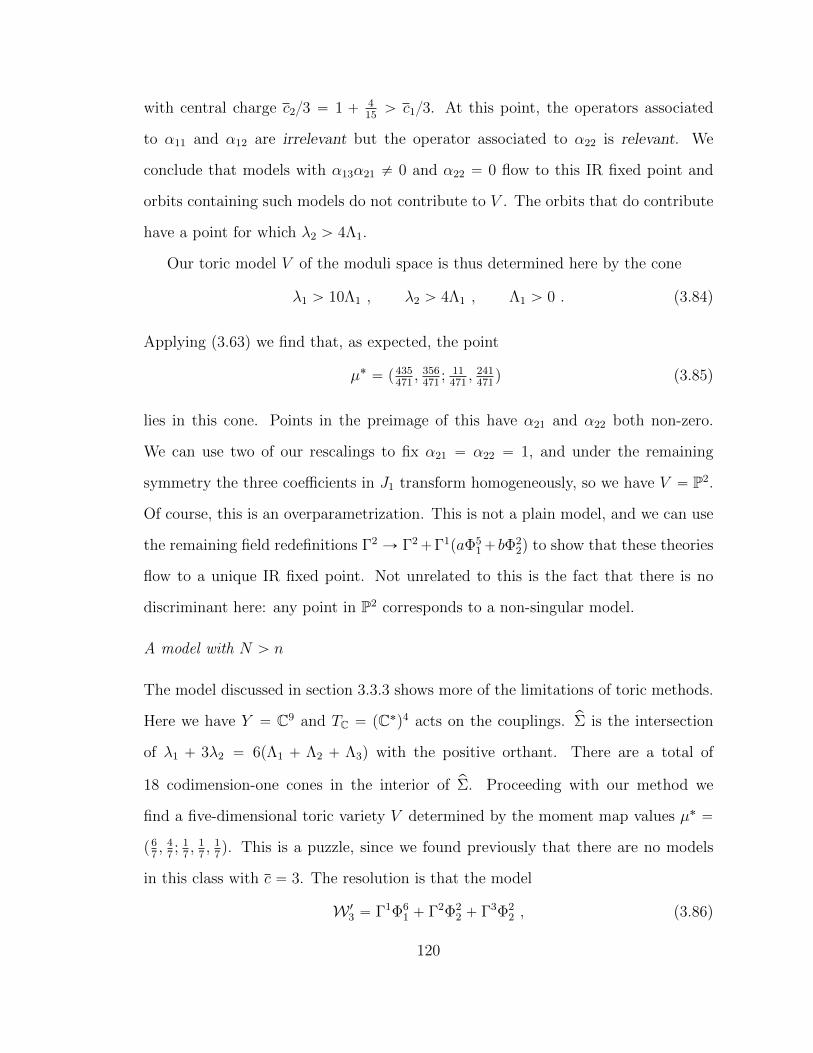
with central charge c23 “ 1 ` 415ą c13. At this point, the operators associated
to α11 and α12 are irrelevant but the operator associated to α22 is relevant. We
conclude that models with α13α21 ‰ 0 and α22 “ 0 flow to this IR fixed point and
orbits containing such models do not contribute to V . The orbits that do contribute
have a point for which λ2 ą 4Λ1.
Our toric model V of the moduli space is thus determined here by the cone
λ1 ą 10Λ1 , λ2 ą 4Λ1 , Λ1 ą 0 . (3.84)
Applying (3.63) we find that, as expected, the point
µ˚ “ p435471, 356
471; 11
471, 241
471q (3.85)
lies in this cone. Points in the preimage of this have α21 and α22 both non-zero.
We can use two of our rescalings to fix α21 “ α22 “ 1, and under the remaining
symmetry the three coefficients in J1 transform homogeneously, so we have V “ P2.
Of course, this is an overparametrization. This is not a plain model, and we can use
the remaining field redefinitions Γ2 Ñ Γ2`Γ1paΦ51`bΦ
22q to show that these theories
flow to a unique IR fixed point. Not unrelated to this is the fact that there is no
discriminant here: any point in P2 corresponds to a non-singular model.
A model with N ą n
The model discussed in section 3.3.3 shows more of the limitations of toric methods.
Here we have Y “ C9 and TC “ pC˚q4 acts on the couplings. pΣ is the intersection
of λ1 ` 3λ2 “ 6pΛ1 ` Λ2 ` Λ3q with the positive orthant. There are a total of
18 codimension-one cones in the interior of pΣ. Proceeding with our method we
find a five-dimensional toric variety V determined by the moment map values µ˚ “
p67, 4
7; 1
7, 1
7, 1
7q. This is a puzzle, since we found previously that there are no models
in this class with c “ 3. The resolution is that the model
W 13 “ Γ1Φ6
1 ` Γ2Φ22 ` Γ3Φ2
2 , (3.86)
120
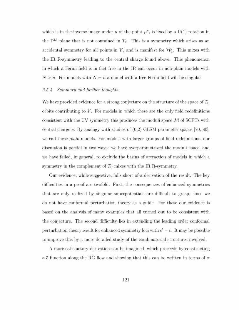
which is in the inverse image under µ of the point µ˚, is fixed by a Up1q rotation in
the Γ2,3 plane that is not contained in TC. This is a symmetry which arises as an
accidental symmetry for all points in V , and is manifest for W 13. This mixes with
the IR R-symmetry leading to the central charge found above. This phenomenon
in which a Fermi field is in fact free in the IR can occur in non-plain models with
N ą n. For models with N “ n a model with a free Fermi field will be singular.
3.5.4 Summary and further thoughts
We have provided evidence for a strong conjecture on the structure of the space of TC
orbits contributing to V . For models in which these are the only field redefinitions
consistent with the UV symmetry this produces the moduli spaceM of SCFTs with
central charge c. By analogy with studies of (0,2) GLSM parameter spaces [70, 80],
we call these plain models. For models with larger groups of field redefinitions, our
discussion is partial in two ways: we have overparametrized the moduli space, and
we have failed, in general, to exclude the basins of attraction of models in which a
symmetry in the complement of TC mixes with the IR R-symmetry.
Our evidence, while suggestive, falls short of a derivation of the result. The key
difficulties in a proof are twofold. First, the consequences of enhanced symmetries
that are only realized by singular superpotentials are difficult to grasp, since we
do not have conformal perturbation theory as a guide. For these our evidence is
based on the analysis of many examples that all turned out to be consistent with
the conjecture. The second difficulty lies in extending the leading order conformal
perturbation theory result for enhanced symmetry loci with c1 “ c. It may be possible
to improve this by a more detailed study of the combinatorial structures involved.
A more satisfactory derivation can be imagined, which proceeds by constructing
a c function along the RG flow and showing that this can be written in terms of α
121
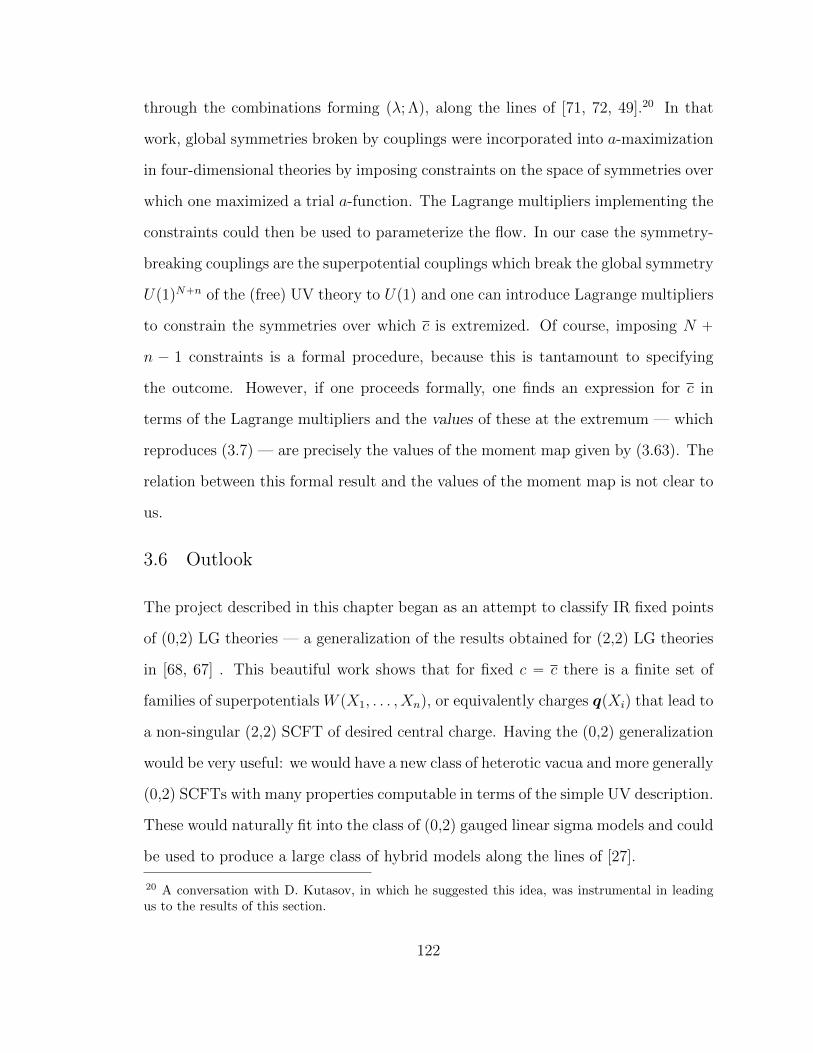
through the combinations forming pλ; Λq, along the lines of [71, 72, 49].20 In that
work, global symmetries broken by couplings were incorporated into a-maximization
in four-dimensional theories by imposing constraints on the space of symmetries over
which one maximized a trial a-function. The Lagrange multipliers implementing the
constraints could then be used to parameterize the flow. In our case the symmetry-
breaking couplings are the superpotential couplings which break the global symmetry
Up1qN`n of the (free) UV theory to Up1q and one can introduce Lagrange multipliers
to constrain the symmetries over which c is extremized. Of course, imposing N `
n ´ 1 constraints is a formal procedure, because this is tantamount to specifying
the outcome. However, if one proceeds formally, one finds an expression for c in
terms of the Lagrange multipliers and the values of these at the extremum — which
reproduces (3.7) — are precisely the values of the moment map given by (3.63). The
relation between this formal result and the values of the moment map is not clear to
us.
3.6 Outlook
The project described in this chapter began as an attempt to classify IR fixed points
of (0,2) LG theories — a generalization of the results obtained for (2,2) LG theories
in [68, 67] . This beautiful work shows that for fixed c “ c there is a finite set of
families of superpotentials W pX1, . . . , Xnq, or equivalently charges qpXiq that lead to
a non-singular (2,2) SCFT of desired central charge. Having the (0,2) generalization
would be very useful: we would have a new class of heterotic vacua and more generally
(0,2) SCFTs with many properties computable in terms of the simple UV description.
These would naturally fit into the class of (0,2) gauged linear sigma models and could
be used to produce a large class of hybrid models along the lines of [27].
20 A conversation with D. Kutasov, in which he suggested this idea, was instrumental in leadingus to the results of this section.
122
What we learned is that, in contrast to the (2,2) case, it is not enough to classify
non-singular (0,2) potentials realizing a particular set of Up1qLˆUp1qR charges. For
instance, the model studied section 3.3.3 would naively realize a c “ 4, c “ 3 (0,2)
SCFT that could correspond to some rather exotic 8-dimensional heterotic vacuum.
In fact no such IR fixed point is obtained for any choice of the UV parameters. This is
a general lesson for building UV models of (0,2) SCFTs: a check of UV R-symmetry
anomalies is not enough, and while the UV theory may well flow somewhere (i.e
to an SCFT with c ą 0), it may wind up far (i.e. at infinite distance) from the
expectations of the model builder. We expect this to be a general lesson applicable
to the wider class of gauged linear sigma models. In exploring that latter point it
should be interesting to study in detail GLSMs with LG phases that exhibit accidents
and extrapolate their consequences to large radius geometries.
For a class of models—the plain LG theories—we were able to obtain a com-
pelling conjecture for a global description of the (0,2) moduli spaceM realizing the
expected central charge. While the resulting combinatorial structure is consistent
with a case-by-case analysis of field redefinitions and their orbits in examples, we
were not able to prove it in generality. Progress on both testing and proving the
conjecture could be made by developing a better understanding of the combinatorial
structure of quasi-homogeneous (0,2) superpotentials, as well as developing Lagrange
multiplier techniques and trial c functions. A classification of plain LG theories seems
achievable; this would yield a large playground to explore LG RG flows and could give
hints to the more general classification problem. Finally, it should be illuminating
to relate our work to studies of RG flows with redundant couplings, e.g. [21].
123
4
Worldsheet instantons and linear models
4.1 Introduction
A natural starting point for exploring the moduli space of (0,2) heterotic compactifi-
cations is the study of the geometry of holomorphic vector bundles V over Calabi-Yau
(CY) manifolds M . Under suitable conditions such bundles determine, to all orders
in α1, a supersymmetric heterotic vacuum. For a long time it has been known [35]
that worldsheet instantons wrapping rational curves in M in principle generate a
potential which destabilizes the vacuum. In rather special cases, such as models
with (2,2) supersymmetry [42] or some specially fine-tuned (0,2) models [38, 40], the
correction terms vanish for each instanton separately, but this is not true in more
generic models [24, 31, 7].
In this context, heterotic compactifications obtained as gauged linear sigma mod-
els (GLSMs) [97] have received special attention, as they are believed to be stable
under worldsheet instantons, even in the generic case in which the contributions of
individual instantons do not vanish. This claim is then a nontrivial vanishing theo-
rem about the total contribution from each instanton class. This was first proposed
124
in [91] and further studied in [17] 1. This work suggests that in these models the
corrections vanish even when the contributions of individual instantons do not. If
true, this would guarantee the existence of a vast playground for tackling issues of
(0,2) moduli spaces.
Essentially, these arguments rely on the fact that in heterotic vacua determined by
(0,2) theories the space-time superpotential for gauge singlets can be determined by
a correlator C computed in a (half-) twisted version of the model. Unlike the twisted
versions of (2,2) theories, this is not a topological field theory, but the simplifications
associated with the existence of a nilpotent scalar charge, such as the decoupling of
exact operators from the correlators of closed operators, carry over to this case and
show that C depends holomorphically on the relevant worldsheet couplings.
This holomorphy together with compactness arguments can be used to show that
the correlator vanishes identically. The argument of [91] used the fact that the
parameter space of the GLSM is compact (or has a natural compactification). C
was shown to be a global section of a holomorphic bundle of negative curvature. If
nonzero, this must exhibit poles, which in this theory arise from the finite-energy
configurations with very large field values which occur at special loci in the parameter
space. At these loci the model is indeed singular, but the large-field region can be
studied semiclassically to demonstrate that these configurations do not lead to any
singularities in C. The absence of poles shows that this vanishes identically. This
was pursued explicitly in a simple example, but the argument did not appear to rely
on details of this example so seemed likely to generalize.
In turn, the argument of [17] relied on the compactness of an appropriate moduli
space of instantons. More precisely, these authors used the fact that the contribu-
tion to C at any fixed instanton number can be related to a calculation in a model
in which many of the worldsheet couplings vanish. In this model, the moduli space
1 In [16] an argument along rather different lines was pursued.
125
of instantons is compact, and a zero-mode counting argument shows that the contri-
bution to C vanishes. Here too, detailed calculations were done in simple examples
but the argument seemed very robust and likely to hold in general.
In this chapter, we follow up on this work with a systematic study of the condi-
tions under which the vanishing theorem of [17] applies. We find that in a generic
gauged linear sigma model the argument that the moduli space of instantons is com-
pact fails, reviving the question of whether these models are in fact destabilized
by worldsheet instantons. We do not resolve this question. We are, however, able
to construct an extensive class of models for which the argument holds – a sizable
playground, if not as extensive as had been hoped.
The rest of the chapter is organized as follows. In Section 4.2 we review the
construction of (0,2) linear models relevant for our analysis. In Section 4.3 we show
that there exist models for which the vanishing of the space-time superpotential for
gauge singlets is not guaranteed and we present an example in detail. In Section
4.4 we prove a vanishing theorem for a particular subclass of (0,2) linear models. In
Section 4.5 we end with some implications of this work and future directions.
4.2 The linear model
Our tool for investigating the issue of instanton corrections in this chapter is the
(0,2) gauged linear sigma model. For a suitably constructed bundle V on a CY space
M presented as a complete intersection HA “ 0 in a Fano toric variety V ,2 the IR
worldsheet dynamics is expected to be the same as that of an Abelian gauge theory
with (0,2) supersymmetry. In this section we are going to review the construction
of the (0,2) linear model [97] in order to establish notation and define the class of
models we consider. More details can be found in appendix C.1.
The linear models we consider are gauge theories with gauge group Up1qR, along
2 We recall that a variety V is Fano if and only if the anticanonical bundle KV of V is ample.
126
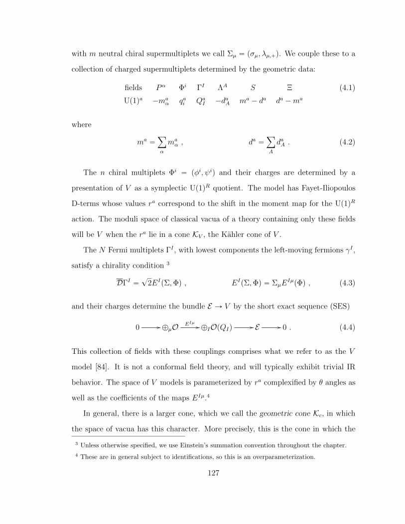
with m neutral chiral supermultiplets we call Σµ “ pσµ, λµ,`q. We couple these to a
collection of charged supermultiplets determined by the geometric data:
fields Pα Φi ΓI ΛA S Ξ
Up1qa ´maα qai Qa
I ´daA ma ´ da da ´ma
(4.1)
where
ma“ÿ
α
maα , da “
ÿ
A
daA . (4.2)
The n chiral multiplets Φi “ pφi, ψiq and their charges are determined by a
presentation of V as a symplectic Up1qR quotient. The model has Fayet-Iliopoulos
D-terms whose values ra correspond to the shift in the moment map for the Up1qR
action. The moduli space of classical vacua of a theory containing only these fields
will be V when the ra lie in a cone KV , the Kahler cone of V .
The N Fermi multiplets ΓI , with lowest components the left-moving fermions γI ,
satisfy a chirality condition 3
DΓI “?
2EIpΣ,Φq , EI
pΣ,Φq “ ΣµEIµpΦq , (4.3)
and their charges determine the bundle E Ñ V by the short exact sequence (SES)
0 // ‘µO EIµ // ‘IOpQIq // E // 0 . (4.4)
This collection of fields with these couplings comprises what we refer to as the V
model [84]. It is not a conformal field theory, and will typically exhibit trivial IR
behavior. The space of V models is parameterized by ra complexified by θ angles as
well as the coefficients of the maps EIµ.4
In general, there is a larger cone, which we call the geometric cone Kc, in which
the space of vacua has this character. More precisely, this is the cone in which the
3 Unless otherwise specified, we use Einstein’s summation convention throughout the chapter.
4 These are in general subject to identifications, so this is an overparameterization.
127
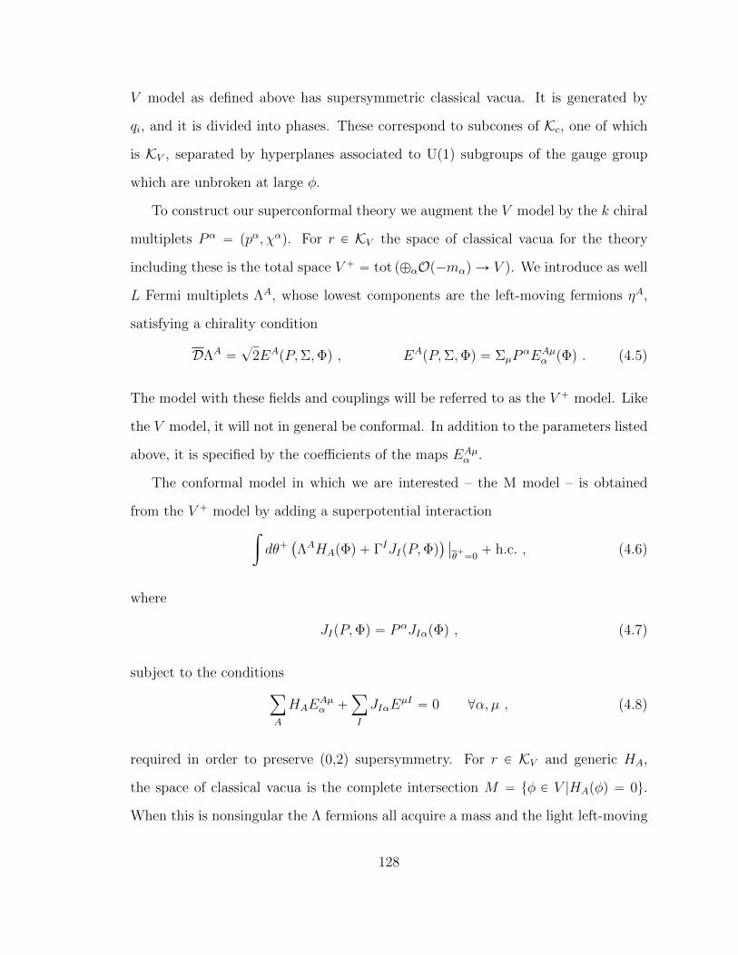
V model as defined above has supersymmetric classical vacua. It is generated by
qi, and it is divided into phases. These correspond to subcones of Kc, one of which
is KV , separated by hyperplanes associated to Up1q subgroups of the gauge group
which are unbroken at large φ.
To construct our superconformal theory we augment the V model by the k chiral
multiplets Pα “ ppα, χαq. For r P KV the space of classical vacua for the theory
including these is the total space V ` “ tot p‘αOp´mαq Ñ V q. We introduce as well
L Fermi multiplets ΛA, whose lowest components are the left-moving fermions ηA,
satisfying a chirality condition
DΛA“?
2EApP,Σ,Φq , EA
pP,Σ,Φq “ ΣµPαEAµ
α pΦq . (4.5)
The model with these fields and couplings will be referred to as the V ` model. Like
the V model, it will not in general be conformal. In addition to the parameters listed
above, it is specified by the coefficients of the maps EAµα .
The conformal model in which we are interested – the M model – is obtained
from the V ` model by adding a superpotential interaction
ż
dθ``
ΛAHApΦq ` ΓIJIpP,Φq˘ ˇ
ˇ
θ`“0` h.c. , (4.6)
where
JIpP,Φq “ PαJIαpΦq , (4.7)
subject to the conditions
ÿ
A
HAEAµα `
ÿ
I
JIαEµI“ 0 @α, µ , (4.8)
required in order to preserve (0,2) supersymmetry. For r P KV and generic HA,
the space of classical vacua is the complete intersection M “ tφ P V |HApφq “ 0u.
When this is nonsingular the Λ fermions all acquire a mass and the light left-moving
128
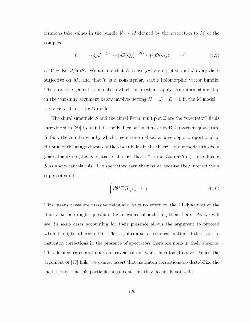
fermions take values in the bundle V Ñ M defined by the restriction to M of the
complex
0 // ‘µO EIµ // ‘IOpQIqJIα // ‘αOpmαq // 0 , (4.9)
as V “ Ker JImE. We assume that E is everywhere injective and J everywhere
surjective on M , and that V is a nonsingular, stable holomorphic vector bundle.
These are the geometric models to which our methods apply. An intermediate step
in the vanishing argument below involves setting H “ J “ E “ 0 in the M model –
we refer to this as the O model.
The chiral superfield S and the chiral Fermi multiplet Ξ are the “spectator” fields
introduced in [39] to maintain the Kahler parameters ra as RG invariant quantities.
In fact, the counterterm by which r gets renormalized at one-loop is proportional to
the sum of the gauge charges of the scalar fields in the theory. In our models this is in
general nonzero (this is related to the fact that V ` is not Calabi–Yau). Introducing
S as above cancels this. The spectators earn their name because they interact via a
superpotential
ż
dθ`ΞSˇ
ˇ
θ`“0` h.c. . (4.10)
This means these are massive fields and have no effect on the IR dynamics of the
theory, so one might question the relevance of including them here. As we will
see, in some cases accounting for their presence allows the argument to proceed
where it might otherwise fail. This is, of course, a technical matter. If there are no
instanton corrections in the presence of spectators there are none in their absence.
This demonstrates an important caveat to our work, mentioned above. When the
argument of [17] fails, we cannot assert that instanton corrections do destabilize the
model, only that this particular argument that they do not is not valid.
129
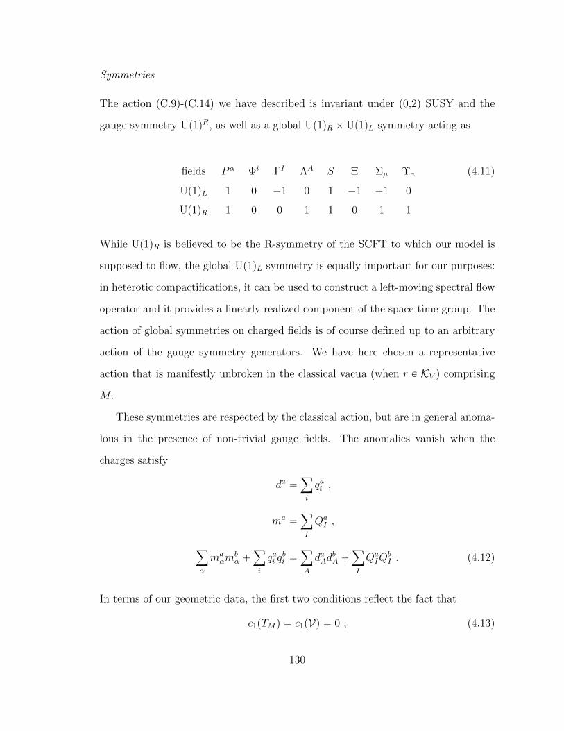
Symmetries
The action (C.9)-(C.14) we have described is invariant under (0,2) SUSY and the
gauge symmetry Up1qR, as well as a global Up1qR ˆ Up1qL symmetry acting as
fields Pα Φi ΓI ΛA S Ξ Σµ Υa
Up1qL 1 0 ´1 0 1 ´1 ´1 0
Up1qR 1 0 0 1 1 0 1 1
(4.11)
While Up1qR is believed to be the R-symmetry of the SCFT to which our model is
supposed to flow, the global Up1qL symmetry is equally important for our purposes:
in heterotic compactifications, it can be used to construct a left-moving spectral flow
operator and it provides a linearly realized component of the space-time group. The
action of global symmetries on charged fields is of course defined up to an arbitrary
action of the gauge symmetry generators. We have here chosen a representative
action that is manifestly unbroken in the classical vacua (when r P KV ) comprising
M .
These symmetries are respected by the classical action, but are in general anoma-
lous in the presence of non-trivial gauge fields. The anomalies vanish when the
charges satisfy
da “ÿ
i
qai ,
ma“ÿ
I
QaI ,
ÿ
α
maαm
bα `
ÿ
i
qai qbi “
ÿ
A
daAdbA `
ÿ
I
QaIQ
bI . (4.12)
In terms of our geometric data, the first two conditions reflect the fact that
c1pTMq “ c1pVq “ 0 , (4.13)
130
while the quadratic condition implies
ch2pTMq “ ch2pVq . (4.14)
Under these conditions, the M model is believed to flow at low energies to a nontrivial
superconformal field theory which is in the same moduli space as the nonlinear
sigma model determined by the pair pM,Vq. Nonperturbative effects (worldsheet
instantons) which can destroy conformal invariance are captured by GLSM gauge
instantons, which are the subject of our investigation here.
4.3 The argument
Let us first review the argument prescribed in [17] for the vanishing of the instanton
contributions to the superpotential W for space-time gauge singlets in a (0,2) linear
sigma model.
The goal is to probe for a background space-time superpotential W . A simple
and direct way to achieve this is to compute the correlator Cabc “ xRaRbRcy, where
Ra is the vertex operator representative for the Kahler modulus Ra of V . In fact, for
each instanton the exponential factor eI0 , where I0 is the instanton classical action,
contains all the dependence on Ra [35, 37]. The correlator Cabc computes the third
derivatives of W with respect to Ra, thus it determines W up to quadratic terms
in the Ra. These terms are forbidden by standard α1 non-renormalization theorems,
hence Cabc determines W directly.
The computation is most easily done in the half-twisted model (see appendix
C.2). In this model, the supercharge Q` becomes a nilpotent scalar symmetry gen-
erator, and correlators of Q`-closed operators can be computed in its cohomology.
On a genus-zero worldsheet, the twist can be realized by spectral flow insertions
and calculations in the twisted model produce suitable correlators of the untwisted
(physical) model.
131
In order to determine the linear model representative of the space-time mode Ra
we restrict our attention to the (0,2) gauge multiplets. In fact, Ra appears in the
linear model through a F-I term. Moreover, gauge singlets must have qL “ 0 and
bosonic vertex operators have qR “ 1. Finally,
Q`λa,´ “ 0 , Q`λa,´ “1
2pDa ´ ifa,01q (4.15)
determine Ra “ λa,´.
The first step of the argument is to show that Cabc vanishes in the O model.
The idea is that the theory without superpotential has a very large symmetry,
G “ Up1q‘pn`N`k`L`2q, where each matter superfield is rotated separately, and the
vertex operators Ra are invariant under this. This symmetry is generically broken
by superpotential couplings down to Up1qL. If the zero-mode path integral measure
5 in nontrivial topological sectors turns out not to be invariant under G, i.e. the
symmetry is anomalous, then contributions to the invariant correlator Cabc from this
sector will vanish. In practice, we follow [17] and construct a Up1q subgroup of
G that is rendered anomalous in all topological sectors by the twisting procedure,
demonstrating that Cabc “ 0 identically in the O model.
The second step uses the fact that Cabc depends holomorphically on J, H and E.
One can then examine the contribution at arbitrary order in an expansion in these
couplings. If there is no term that can possibly absorb the fermion zero-modes in
the anomalous measure, then the correlator vanishes identically. This computation
can be performed in each topological sector of the path integral.
In the untwisted model, the limiting point J “ H “ E “ 0 is of course highly
singular. Both σ and p acquire zero-modes and the space of classical vacua is non-
compact. Such a singularity can invalidate the order-by-order calculation described
5 We recall that the path integral for a correlator of Q`-invariant operators localizes on fixed lociof Q`, given by zero-modes.
132
above. The key observation of [17] is that in suitable examples these dangerous zero-
modes are absent in the half-twisted model. For example, the bosons σ always have
zero-modes, but in the twisted model (see appendix C.2) these fields acquire a spin
and their zero-modes are absent. In general, as we shall see below, p zero-modes are
not completely removed by the twisting.
Another approach was presented in [17], where the vanishing of Cabc at any in-
stanton number follows from an appropriate counting of fermi zero-modes in the
half-twisted model. This was applied in detail for heterotic compactifications de-
scribed by half-linear sigma models, but it also extends to linear models as well.
However, as pointed out above, the same assumption of compactness is required for
this argument to be valid. For definiteness, we present our analysis of the linear
model following the approach of [17] reviewed above, as our results will not depend
on this choice.
4.3.1 The quintic
Let us review how all of this works for the linear model describing the deformations
of the tangent bundle TM over the quintic hypersurface M in V “ P4. The gauge
charges for the (2,2) multiplets Φi “ pΦi,Γiq and P “ pP,Λq are
fields P Φ1 Φ2 Φ3 Φ4 Φ5
Up1q ´5 1 1 1 1 1
(4.16)
The Kahler cone KV “ Kc here is simply given by r ě 0 and the relevant instantons
are defined by K_V “ tn ě 0u. The O model has as a target space the total space
of the anticanonical bundle on V , tot pOp´5q Ñ P4q. First of all, we check that the
moduli space of gauge instantons for this model is compact. Indeed, we verify that
there are no holomorphic sections of
p Ø ΓpK12 bOp´5nqq , (4.17)
133
and thus p has no zero-modes. This, together with the fact that there are no zero-
modes of σ shows that the space of zero-modes is compact in any topological sector.
Next, by looking at the degree of the line bundles of the half-twisted model in (C.21)
we see that the relevant fermions zero-modes are
fields ψi
γi η χ
bundle Opnq Opn´ 1q Op5nq Op5n´ 1q
# z.m. n` 1 n 5n` 1 5n
(4.18)
The fermion contribution to the zero-mode path-integral measure is then given by
dµF “ dλ´dηdχź
i
dψidγi . (4.19)
Now, the O model is invariant under a symmetry Up1qC which assigns charge `1
to the multiplets Φi and leaves everything else invariant. Under this symmetry the
measure above transforms with charge `5. Hence, the correlator C vanishes in the
O model. The holomorphic superpotential couplings are given by
LYuk
ˇ
ˇ
J“H“E“0“ ´γiEiλ` ` γ
iJiχ` ηH,jψj , (4.20)
where H is a quintic polynomial defining the hypersurface M , Ji are generic quartic
polynomials and Ei are generic linear polynomials subject to (4.8). Clearly, each
coupling transforms under Up1qC with either charge +5 or is neutral. By the argu-
ment above the correlator C vanishes in the full theory and there are no instanton
corrections to the space-time superpotential.
4.3.2 A counter-example
Let us consider a two-parameter model with the following charge assignments
fields Φ1,2,3 Φ4,5 Φ6,7 Λ1 Λ2 Γ1,2 Γ3 Γ4,5,6,7 P 1 P 2
Up1q1 1 1 0 ´3 ´2 2 1 0 ´4 ´1
Up1q2 1 0 1 ´3 ´2 0 1 1 ´2 ´3
(4.21)
134
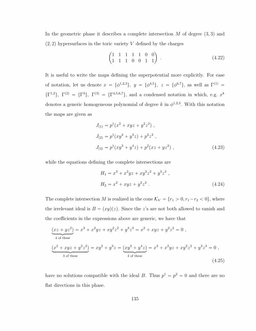
In the geometric phase it describes a complete intersection M of degree p3, 3q and
p2, 2q hypersurfaces in the toric variety V defined by the charges
ˆ
1 1 1 1 1 0 01 1 1 0 0 1 1
˙
. (4.22)
It is useful to write the maps defining the superpotential more explicitly. For ease
of notation, let us denote x “ tφ1,2,3u, y “ tφ4,5u, z “ tφ6,7u, as well as Γp1q “
tΓ1,2u, Γp2q “ tΓ3u, Γp3q “ tΓ4,5,6,7u, and a condensed notation in which, e.g. xk
denotes a generic homogeneous polynomial of degree k in φ1,2,3. With this notation
the maps are given as
Jp1q “ p1px2
` xyz ` y2z2q ,
Jp2q “ p1pxy2
` y3zq ` p2z2 ,
Jp3q “ p1pxy3
` y4zq ` p2pxz ` yz2
q , (4.23)
while the equations defining the complete intersections are
H1 “ x3` x2yz ` xy2z2
` y3z3 ,
H2 “ x2` xyz ` y2z2 . (4.24)
The complete intersection M is realized in the cone KV “ tr1 ą 0, r1´r2 ă 0u, where
the irrelevant ideal is B “ pxyqpzq. Since the z’s are not both allowed to vanish and
the coefficients in the expressions above are generic, we have that
pxz ` yz2q
loooomoooon
4 of these
“ x3` x2yz ` xy2z2
` y3z3“ x2
` xyz ` y2z2“ 0 ,
px2` xyz ` y2z2
qloooooooooomoooooooooon
3 of these
“ xy2` y3z “ pxy3
` y4zqlooooomooooon
4 of these
“ x3` x2yz ` xy2z2
` y3z3“ 0 ,
(4.25)
have no solutions compatible with the ideal B. Thus p1 “ p2 “ 0 and there are no
flat directions in this phase.
135
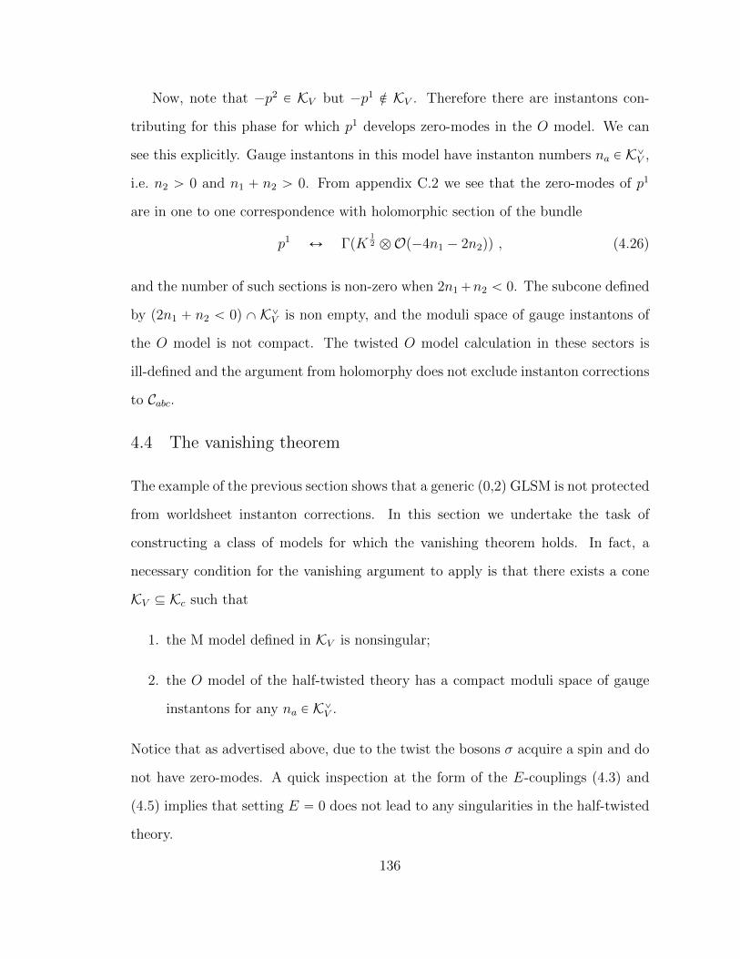
Now, note that ´p2 P KV but ´p1 R KV . Therefore there are instantons con-
tributing for this phase for which p1 develops zero-modes in the O model. We can
see this explicitly. Gauge instantons in this model have instanton numbers na P K_V ,
i.e. n2 ą 0 and n1 ` n2 ą 0. From appendix C.2 we see that the zero-modes of p1
are in one to one correspondence with holomorphic section of the bundle
p1Ø ΓpK
12 bOp´4n1 ´ 2n2qq , (4.26)
and the number of such sections is non-zero when 2n1`n2 ă 0. The subcone defined
by p2n1 ` n2 ă 0q X K_V is non empty, and the moduli space of gauge instantons of
the O model is not compact. The twisted O model calculation in these sectors is
ill-defined and the argument from holomorphy does not exclude instanton corrections
to Cabc.
4.4 The vanishing theorem
The example of the previous section shows that a generic (0,2) GLSM is not protected
from worldsheet instanton corrections. In this section we undertake the task of
constructing a class of models for which the vanishing theorem holds. In fact, a
necessary condition for the vanishing argument to apply is that there exists a cone
KV Ď Kc such that
1. the M model defined in KV is nonsingular;
2. the O model of the half-twisted theory has a compact moduli space of gauge
instantons for any na P K_V .
Notice that as advertised above, due to the twist the bosons σ acquire a spin and do
not have zero-modes. A quick inspection at the form of the E-couplings (4.3) and
(4.5) implies that setting E “ 0 does not lead to any singularities in the half-twisted
theory.
136
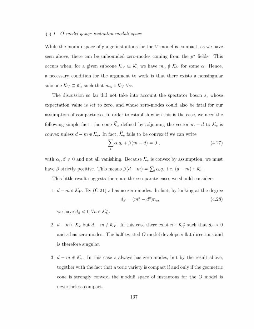
4.4.1 O model gauge instanton moduli space
While the moduli space of gauge instantons for the V model is compact, as we have
seen above, there can be unbounded zero-modes coming from the pα fields. This
occurs when, for a given subcone KV Ď Kc we have mα R KV for some α. Hence,
a necessary condition for the argument to work is that there exists a nonsingular
subcone KV Ď Kc such that mα P KV @α.
The discussion so far did not take into account the spectator boson s, whose
expectation value is set to zero, and whose zero-modes could also be fatal for our
assumption of compactness. In order to establish when this is the case, we need the
following simple fact: the cone pKc defined by adjoining the vector m ´ d to Kc is
convex unless d´m P Kc. In fact, pKc fails to be convex if we can writeÿ
i
αiqi ` βpm´ dq “ 0 , (4.27)
with αi, β ě 0 and not all vanishing. Because Kc is convex by assumption, we must
have β strictly positive. This means βpd´mq “ř
i αiqi, i.e. pd´mq P Kc.
This little result suggests there are three separate cases we should consider:
1. d´m P KV . By (C.21) s has no zero-modes. In fact, by looking at the degree
dS “ pma´ daqna, (4.28)
we have dS ď 0 @n P K_V .
2. d´m P Kc but d´m R KV . In this case there exist n P K_V such that dS ą 0
and s has zero-modes. The half-twisted O model develops s-flat directions and
is therefore singular.
3. d ´ m R Kc. In this case s always has zero-modes, but by the result above,
together with the fact that a toric variety is compact if and only if the geometric
cone is strongly convex, the moduli space of instantons for the O model is
nevertheless compact.
137
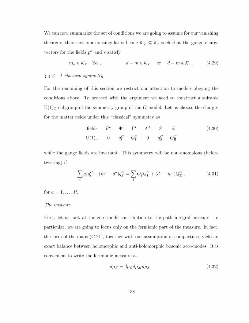
We can now summarize the set of conditions we are going to assume for our vanishing
theorem: there exists a nonsingular subcone KV Ď Kc such that the gauge charge
vectors for the fields pα and s satisfy
mα P KV @α , d´m P KV or d´m R Kc . (4.29)
4.4.2 A classical symmetry
For the remaining of this section we restrict our attention to models obeying the
conditions above. To proceed with the argument we need to construct a suitable
Up1qC subgroup of the symmetry group of the O model. Let us choose the charges
for the matter fields under this “classical” symmetry as
fields Pα Φi ΓI ΛA S Ξ
Up1qC 0 qCi QCI 0 qCS QC
Ξ
(4.30)
while the gauge fields are invariant. This symmetry will be non-anomalous (before
twisting) if
ÿ
i
qai qCi ` pm
a´ daqqCS “
ÿ
I
QaIQ
CI ` pd
a´ma
qQCΞ , (4.31)
for a “ 1, . . . , R.
The measure
First, let us look at the zero-mode contribution to the path integral measure. In
particular, we are going to focus only on the fermionic part of the measure. In fact,
the form of the maps (C.21), together with our assumption of compactness yield an
exact balance between holomorphic and anti-holomorphic bosonic zero-modes. It is
convenient to write the fermionic measure as
dµF “ dµGdµMdµS , (4.32)
138
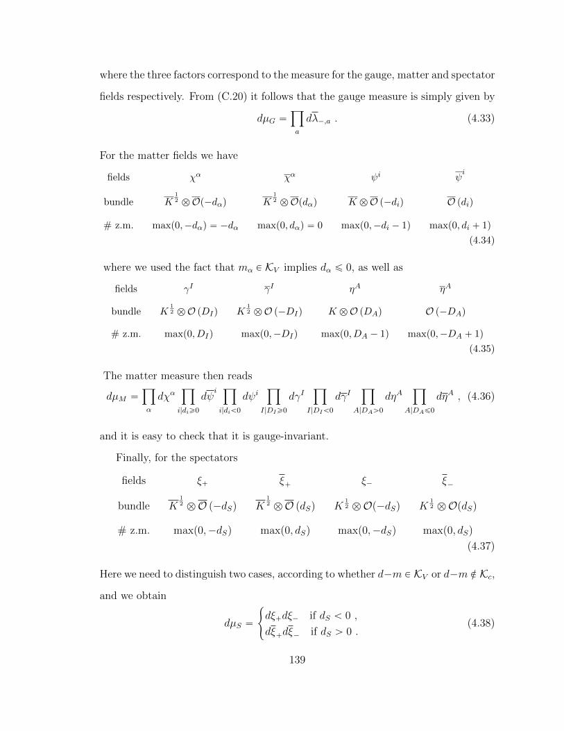
where the three factors correspond to the measure for the gauge, matter and spectator
fields respectively. From (C.20) it follows that the gauge measure is simply given by
dµG “ź
a
dλ´,a . (4.33)
For the matter fields we have
fields χα χα ψi ψi
bundle K12 bOp´dαq K
12 bOpdαq K bO p´diq O pdiq
# z.m. maxp0,´dαq “ ´dα maxp0, dαq “ 0 maxp0,´di ´ 1q maxp0, di ` 1q
(4.34)
where we used the fact that mα P KV implies dα ď 0, as well as
fields γI γI ηA ηA
bundle K12 bO pDIq K
12 bO p´DIq K bO pDAq O p´DAq
# z.m. maxp0, DIq maxp0,´DIq maxp0, DA ´ 1q maxp0,´DA ` 1q
(4.35)
The matter measure then reads
dµM “ź
α
dχαź
i|diě0
dψi ź
i|diă0
dψiź
I|DIě0
dγIź
I|DIă0
dγIź
A|DAą0
dηAź
A|DAď0
dηA , (4.36)
and it is easy to check that it is gauge-invariant.
Finally, for the spectators
fields ξ` ξ` ξ´ ξ´
bundle K12 bO p´dSq K
12 bO pdSq K
12 bOp´dSq K
12 bOpdSq
# z.m. maxp0,´dSq maxp0, dSq maxp0,´dSq maxp0, dSq
(4.37)
Here we need to distinguish two cases, according to whether d´m P KV or d´m R Kc,
and we obtain
dµS “
#
dξ`dξ´ if dS ă 0 ,
dξ`dξ´ if dS ą 0 .(4.38)
139
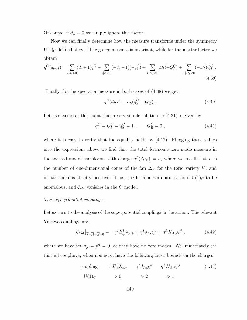
Of course, if dS “ 0 we simply ignore this factor.
Now we can finally determine how the measure transforms under the symmetry
Up1qC defined above. The gauge measure is invariant, while for the matter factor we
obtain
qCpdµM q “ÿ
i|diě0
pdi ` 1qqCi `ÿ
i|diă0
p´di ´ 1qp´qCi q `ÿ
I|DIě0
DIp´QCI q `
ÿ
I|DIă0
p´DIqQCI .
(4.39)
Finally, for the spectator measure in both cases of (4.38) we get
qCpdµSq “ dSpqCS `Q
CΞ q , (4.40)
Let us observe at this point that a very simple solution to (4.31) is given by
qCi “ QCI “ qCS “ 1 , QC
Ξ “ 0 , (4.41)
where it is easy to verify that the equality holds by (4.12). Plugging these values
into the expressions above we find that the total fermionic zero-mode measure in
the twisted model transforms with charge qCpdµF q “ n, where we recall that n is
the number of one-dimensional cones of the fan ∆V for the toric variety V , and
in particular is strictly positive. Thus, the fermion zero-modes cause Up1qC to be
anomalous, and Cabc vanishes in the O model.
The superpotential couplings
Let us turn to the analysis of the superpotential couplings in the action. The relevant
Yukawa couplings are
LYuk
ˇ
ˇ
J“H“E“0“ ´γIEI
,µλµ,` ` γIJIαχ
α` ηAHA,jψ
j , (4.42)
where we have set σµ “ pα “ 0, as they have no zero-modes. We immediately see
that all couplings, when non-zero, have the following lower bounds on the charges
couplings γIEI,µλµ,` γIJIαχ
α ηAHA,jψj
Up1qC ě 0 ě 2 ě 1
(4.43)
140
In particular, we note that these values are all non-negative and therefore it is not
possible to absorb the zero-modes in excess in the measure by bringing down fermion
terms from the action. The correlator Cabc thus vanishes at all orders in the super-
potential couplings, which concludes the proof that instantons do not contribute to
the space-time superpotential in our class of models.
Note that we ignored the anti-holomorphic functions J, H and E in (4.42). This
is in fact legitimate since, as observed above, half-twisted correlators of Q`-closed
operators have a holomorphic dependence on J, H and E.
4.5 Outlook
In this chapter, we investigated the details of the elegant argument of [17] for the
absence of instanton corrections to the space-time superpotential in heterotic com-
pactifications based on (0,2) GLSMs. We have not been able to extend the argument
to the most general case.
The immediate question raised is: are some of these vacua in fact destabilized
by instantons? One clear way to resolve this would be to produce an argument
that holds in more generality. It is possible, however, that no such argument can
be found and that in fact instanton corrections do arise. One way to detect such
corrections would be an indirect approach, in which properties of the solution, such
as the dimension of the space of massless gauge-neutral scalar fields, are compared
at different limiting points in the moduli space. A more direct approach would be
to compute the instanton contributions explicitly. Perhaps the GLSM can provide
a framework within which these calculations, which have proved difficult in general,
are tractable.
On the other hand, we have now an extensive class of (0,2) models which are truly
conformally invariant. These can be used to explore the moduli space of (0,2) theories
without a (2,2) locus, extending recent work that has focused on deformations of
141
(2,2) models [76, 5, 45]. In particular, one could look for special loci, e.g. good
hybrid models [27] or Landau-Ginzburg points and hope to learn something about
the structure of the resulting theories. In particular, hybrid models could be a
promising laboratory for explicit computations of worldsheet instantons, given the
simpler structure of rational curves on the lower dimensional base instead than on a
CY three-fold.
We have shown in Chapter 3 that other “bad” things can happen in (0,2) models
[26]. In particular, it is shown, in the context of Landau-Ginzburg models, that the
common assumption that accidental IR symmetries do not spoil the correspondence
between operators in the IR and the ones in the UV is not guaranteed in (0,2) models.
When this occurs, the structure of the conformal manifold is dramatically modified.
There is a priori no reason that would prevent the same phenomenon from happening
in a generic phase of a GLSM. For example, one could realize one of the “accidental”
LG theories as a phase of a GLSM and study how this pathology is realized in the
geometric phase. This could shed new light on the conditions for the data pM,Vq to
lead to consistent heterotic backgrounds.
142
Appendix A
Hybrid geometry
A.1 An example
Let B “ P1 and take Y to be the total space of X “ Op´2q Ñ P1. We cover Y by
two patches Uu and Uv, with local coordinates pu, φuq and pv, φvq, respectively :
u “ v´1, φu “ v2φv on Uu X Uv “ C˚. (A.1)
The projection π : Y Ñ B is simply pu, φuq Ñ u and pv, φvq Ñ v in the two patches.
The transition function for σ “ σ1uBu ` σ
2uBφu , a section of TY , is
`
σ1u σ2
u
˘
“`
σ1v σ2
v
˘
ˆ
´v´2 2vφv0 v2
˙
. (A.2)
TY belongs to a family of rank 2 holomorphic bundles Vε Ñ Y with transition
function
`
σ1u σ2
u
˘
“`
σ1v σ2
v
˘
Mε , Mε ”
ˆ
´v´2 2εvφv0 v2
˙
. (A.3)
When ε “ 0 the bundle splits: Vε“0 “ π˚Op2q ‘ π˚Op´2q; more generally Vε is an
irreducible rank 2 bundle over Y .
143
An example of a quasi-homogeneous superpotential depending on a parameter α
is
Wu “ pα ` u8qφ4
u , Wv “ pαv8` 1qφ4
v . (A.4)
Clearly Wu “ Wv on the overlap. Computing the gradient in the two patches, we
obtain
dWu “ 8u7φ4udu` 4pα ` u8
qφ3udφu , dWv “ 8αv7φ4
vdv ` 4pαv8` 1qφ3
vdφv .(A.5)
It is then easy to see that for α ‰ 0 we have dW´1p0q “ B. A more general
superpotential respecting the same quasi-homogeneity is
Wu “ Supuqφ4u , Wv “ Svpvqφ
4v , (A.6)
where Su,v is the restriction of Σ P H0pB,Op8qq to Uu,v. The potential condition is
satisfied for generic choices of Σ.
We can see how the fibration affects the naive chiral ring Rp of the LG fiber theory
over a point p P B: dimRp jumps in complex co-dimension 1 but stays finite if the
potential condition is satisfied. In our example Ru “ t1, φu, φ2uu for u8`α ‰ 0, while
at the 8 special points R “ t1, φu, φ2u, φ
3uu. If α “ 0 then the potential condition is
violated, and dimR0 “ 8.
A (0,2) deformation
Taking the left-moving bundle to be E “ Vε, we obtain a class of (0,2) theories. The
most general (0,2) superpotential that respects the same quasi-homogeneity as dW ,
J P ΓpE˚q, takes the form
Ju “
ˆ
Tupuqφ4u
4Supuqφ3u
˙
, Jv “
ˆ
Tvpvqφ4v
4Svpvqφ3v
˙
, (A.7)
where S and T are holomorphic functions constrained by Ju “ M´1ε Jv when u ‰ v.
Su,v are restrictions of Σ as above, while Tu,v are given by
Tupuq “ ´ rΣˇ
ˇ
ˇ
u` 8εu´1
pSupuq ´ Sup0qq , Tvpvq “ rΣˇ
ˇ
ˇ
v` 8εv7Sup0q , (A.8)
144
where rΣ P H0pB,Op6qq. The potential condition is satisfied for generic Σ and rΣ.
Setting ε “ 1 and Tu “ BuSu, we recover the (2,2) potential from above. On the
other hand, taking ε “ 0, we see that T is just given by restriction of holomorphic
sections of Op6q.
We can compare the number of holomorphic deformation parameters in the (2,2)
or (0,2) superpotentials. W depends on 9 holomorphic parameters specifying section
Σ. The more generic (0,2) superpotential J , on the other hand, depends on 16
parameters, independent of ε; as a check, we see that demanding that J is integrable
to W reduces the parameters to 9.
Metrics for Y and E
It is well known that Y admits an ALE Kahler Ricci-flat metric with Kahler poten-
tial 1
KCY “?
1` L`1
2log
?1` L´ 1
?1` L` 1
, L ” 4φφp1` uuq2 . (A.9)
This is obviously well-defined with respect to the patching. To leading order in the
fiber coordinates, we find that up to irrelevant constants
KCY “ K `Op|φ|4q, K “ logp1` uuq ` p1` uuq2φφ . (A.10)
K leads to a complete non-Ricci-flat metric on X:
gX “
ˆ
guu guφgφu gφφ
˙
“
ˆ
p1` uuq´2 ` 2p1` 2uuqφφ 2uφp1` uuq
2uφp1` uuq p1` uuq2
˙
. (A.11)
To Op|φ|4q this agrees with the Kahler metric obtained by symplectic reduction from
C3.
1 Constructions of such metrics for line bundles over Pn´1, which generalize the classic work ofEguchi and Hanson [46], go back to [32, 50]; [55] gives an elegant generalization for line bundlesover symmetric spaces. These are also the only explicitly known ALE metrics with SUpnq n ě 3holonomy [60].
145
We can also endow E with a Hermitian metric. In our example with E “ Vε, a
convenient choice is
pσ, τq ” σGτ , G “ˆ
p1` uuq´2 ` 2εεp1` 2uuqφφ 2εuφp1` uuq
2εuφp1` uuq p1` uuq2
˙
. (A.12)
Setting ε “ 1, we obtain a Hermitian, in fact Kahler, metric on TY . Setting φ “ 0
we obtain the bundles restricted to B. As we might expect, TY |B “ Vε|B “ Op2q ‘
Op´2q.
The explicit Ricci-flat metric on Y is fairly complicated, and generalizations to
other spaces are typically not available. Fortunately, we do not need the explicit
form of the metric for our analysis: by construction the superpotential restricts low
energy field configurations to B, and the details of the metric on Y away from the
base become irrelevant to the IR physics.
A.2 Vertical Killing vectors
In this appendix we examine holomorphic vertical Killing vectors on Y and prove
that with our assumptions they act homogeneously on the fiber directions.
Let V “ V α B
Byα` c.c. be an holomorphic vector field on Y , i.e. V α
,β“ 0. Then
the Killing equation for a Kahler metric gαβ takes the form
BγpgαβVαq ` BβpgγαV
αq “ 0 . (A.13)
Using the base/fiber decomposition yα “ puI , φiq, the hybrid metric has components
gIJ “ GIJ ` φhIJφ, giJ “ himJφm, gI “ φmhmI , gi “ hi . (A.14)
Since V is vertical, we have V “ V i BBφi` c.c., and a moment’s thought shows that
V ipu, φq transforms as a section of π˚pXq. In this case the Killing equation reduces
to
BγpgiβViq ` BβpgγıV
ıq “ 0 , (A.15)
146
and decomposing it further along base/fiber directions leads to two non-trivial con-
ditions. First, from β, γ “ , k we obtain
BkVi` hiBV
ı
hkı “ 0 . (A.16)
Since h is φ-independent and BmVı
“ 0, we conclude that
V i“ Aikpuqφ
k`Bi
puq, Aı
k “ pAikq˚“ ´hıiAki hkk . (A.17)
The latter restriction on A P H0pB,X b X˚q, combined with its holomorphy leads
to DJA “ 0. The remaining non-trivial conditions are obtained by taking β, γ “ J, k
in the Killing equation, and they lead to DJB “ 0 for B P H0pB,Xq.
So, we have learned that vertical automorphic Killing vectors are characterized
by covariantly constant sections A P ΓpX bX˚q and B P ΓpXq, with the additional
restriction
pAikq˚“ ´hıiAki hkk . (A.18)
In fact, we can always shift away the global section B by a redefinition of the φi;
moreover, for a generic choice of metric h the only solution for A is a diagonal anti-
Hermitian u-independent matrix; demanding LVW “ W will fix the eigenvalues (up
to an overall i) to be the charges qi.
A.3 A little sheaf cohomology
In this section we present some useful results for reducing sheaf cohomology on Y
to computations on the base B in the case that X “ ‘iLi. In order to compute Q0
cohomology we need an effective method to evaluate
H‚rpY , π
˚pEq b ^sTY b^tT ˚Y q, (A.19)
where E is some bundle (or more generally sheaf) on B, and r is the restriction to
fine grade r. Recall that the grading r P Zn assigns to every monomialś
i φrii grade
147
r “ pr1, . . . , rnq; in particular φi has grade xi with pxiqj “ δij. Since Y is non-
compact the grade restriction is necessary to obtain a well-posed counting problem.
For instance, the structure sheaf OY clearly has infinite-dimensional cohomology
group H0pY ,OY q.
Graded cohomology of a pulled-back sheaf
Suppose s “ t “ 0 in (A.19). As we now show,
H‚rpY , π
˚pEqq » H‚
pB, E b Lrq, (A.20)
where Lr Ñ B is the line bundle Lr ” bipL˚i qri .
The proof follows from the basic geometry. First, to describe the line bundles
Li Ñ B, we work with a cover U “ tUau for B with local coordinates uIa in each
patch, so that on overlaps Uab ‰ H sections of Li satisfy
λibpubq “ λiapuaqgiabpuaq , (A.21)
where the giab are the transition functions defining the bundle Li. The sections σa of
a sheaf E Ñ B satisfy
σbpubq “ σapuaqGabpuaq , (A.22)
where the Gab are the transition functions for E , and sections of π˚pEq Ñ Y patch
as
σbpub, φbq “ σapua, φaqGabpuaq , (A.23)
with φib “ φiagiabpuaq . Since the transition functions for π˚pEq are identical to the
transition functions for E over B, at fixed grade (A.23) takes the formź
i
pφibqriξbpubq “
ź
i
pφiaqriξapuaqGabpuaq ðñ ξbpubq “ ξapuaqGabpuaq
ź
i
“
giabpuaq‰´ri .
(A.24)
Hence the space of sections of π˚pEqr over Y is isomorphic to the space of sections
of E b Lr over B. The grading is compatible with Cech cohomology (i.e. with
defining chains for higher intersections Ua1¨¨¨ak and taking cohomology of the Cech
differential), and (A.20) holds.
148
The tangent bundle
Having reduced the graded cohomology of a pull-back sheaf to a cohomology problem
on the base, we now turn to the tangent bundle. This is of course not in general the
pull-back of a sheaf from B, as we explictly saw in appendix A.1. However, TY fits
into a short exact sequence
0 // π˚pXq // TY // π˚pTBq // 0 . (A.25)
This is easy to see explicitly. In an open neighborhood Ua a vector field Σ takes the
form
Σa “ VaB
Bua` νa
B
Bφa, (A.26)
and on overlaps Uab
Vb “ VaBubBua, νb “ νagab ` φaLV gab , (A.27)
where gab are the transition functions for X. Hence, we see that a section ν of X
lifts to a section of TY with V “ 0, while a section of TY at φ “ 0 yields a section of
TB.
This short exact sequence can be decomposed with respect to the fine grading.
Working again in the case X “ ‘iLi, the transition functions for sections of TY can
be written explicitly as
pσ0b , σ
1b , . . . , σ
nb q “ pσ
0a, σ
1a, . . . , σ
na q
¨
˚
˚
˚
˚
˚
˝
BubBua
φ1aBg
1ab φ2
aBg2ab ¨ ¨ ¨ φnaBg
nab
0 g1ab 0 ¨ ¨ ¨ 0
0 0 g2ab ¨ ¨ ¨ 0
......
.... . .
...0 0 0 ¨ ¨ ¨ gnab
˛
‹
‹
‹
‹
‹
‚
. (A.28)
Hence, sections of TY also admit a fine grading, which we define
pΣqr ” pσ0r, σ
1r`x1
, σ2r`x2
, . . . , σnr`xnq . (A.29)
This means the short exact sequence for TY can be decomposed according to r as
0 // ‘ipπ˚Liqr`xi
// pTY qr // pπ˚TBqr // 0 . (A.30)
149
Using the induced long exact sequence on cohomology, together with (A.20), we can
evaluate H‚rpY , TY q. Taking appropriate products one can generalize this result to
compute all desired cohomology groups in (A.19).
We should mention one small subtlety in grading the sections of TY : from (A.29)
we see that there can be non-trivial contributions for ri “ ´1. More precisely,
pTY qr “ 0 whenever any ri ă ´1 or ri “ rj “ ´1, and if a single ri “ ´1 we have
pTY qr “ pπ˚Liqr`xi , (A.31)
in which case H‚rpY , TY q “ H‚pB,Lrq.
Application to X “ Op´2q and B “ P1
In this case the grading is one-dimensional r “ prq, the grading bundle is Ls “
pOp´2q˚qs “ Op2sq, and for any r ě 0 the structure sheaf cohomology is
H0r pY ,OY q “ H0
pB,Op2rqq » C2r`1 , Hqr pY ,OY q “ 0, for q ą 0 . (A.32)
For the tangent sheaf the short exact sequence
0 // pπ˚Op´2qqr`1// pTY qr // pπ˚Op2qqr // 0 (A.33)
leads to the long exact sequence in cohomology
0 // H0pB,Op2rqq // H0r pY , TY q // H0pB,Op2r ` 2qq
H1pB,Op2rqq // H1r pY , TY q // H1pB,Op2r ` 2qq // 0
(A.34)
At grade 0 we obtain
0 // C // H00 pY , TY q // C3
0 // H10 pY , TY q // 0 // 0
(A.35)
150
Hence, H00 pY , TY q » C4, and H1
0 pY , TY q “ 0. More generally, for any non-negative
grade
H0r pY , TY q “ H0
r pB,Op2rqq ‘H0r pB,Op2r ` 2qq » C4r`4, H1
r pY , TY q “ 0 .(A.36)
A note on horizontal representatives
In order to evaluate Q0 cohomology we needed to study the finely graded Dolbeault
cohomology of horizontal forms on Y valued in a holomorphic sheaf F . One might
wonder what is the relationship between these horizontal forms and more general
Dolbeault classes in Hp0,uq
BpY ,Fq. In fact, every such class has a horizontal repre-
sentative, which is why our results on finely graded cohomology describe horizontal
Dolbeault cohomolgy as well. This is rather intuitive, since the fiber space is simply
Cn (or CnΓ for orbi-bundles), but for completeness we give a sketch of the proof.2
The statement is trivial at u “ 0, so we consider u “ 1. Let τ P ker B X
Ωp0,1qpY ,OY q. In any patch Ua we have
τa “ ωaIduIa ` σaıdφ
ı
a . (A.37)
We define ηapua, ua, φa, φαq via the line integral
ηα “
ż φa
0
dzıσaıpua, ua, φa, zq . (A.38)
Since Bτ “ 0 implies σaı, “ σa,ı, the line integral does not depend on the choice
of contour from 0 to φ; moreover, a change of variables zı “ gıbayı in the integral
shows that ηa “ ηb on any Uab ‰ H, so that η patches to a function on Y . Therefore
τ 1 “ τ ´ Bη is a (0,1) horizontal form, and a moment’s thought shows that Bτ 1 “ 0
implies that it has a holomorphic dependence on the fiber coordinates.
One can generalize the argument to u ą 1 and more general holomorphic sheaf
2 This essentially follows the standard proof [30] that HkdRpRn,Rq “ 0 for k ą 0.
151

F Ñ Y . The analogous construction yields η, a section of Ωp0,u´1qpY ,Fq, such that
τ 1 “ τ ´ Bη is a horizontal representative of rτ s P Hp0,uq
BpY ,Fq.
A.4 Massless spectrum of a (0,2) CY NLSM
In this appendix we apply the first-order techniques developed in section 2.4.3 to
marginal deformations of (0,2) NLSMs with CY target space B and a left-moving
SUpnq bundle V . We assume ch2pVq “ ch2pTBq and V is a stable bundle. This
ensures that the NLSM is conformally invariant to all orders in α1 perturbation
theory [96, 35]. Our techniques allow us to determine the massless spectrum to all
orders in α1. The results for the (R,R) sector and for the gauge-charged matter
are exactly the same as those obtained by a Born-Oppenheimer approach in [40].
However, the massless gauge-neutral chiral matter has to our best knowledge not
been studied directly in the NLSM. The first-order formulation of Q0 cohomology
turns out to be perfectly suited to this task and should be thought of as a first step
in systematically including any non-perturbative world-sheet effects.
In parallel with the analysis of the k “ 1 sector in section 2.5.2, we first list
the operators that can give rise to massless singlets. We need to slightly alter our
notation in comparison to the TB “ V analysis of section 2.5.2; just in this appendix
we use I, J, . . . for tangent/cotangent indices, while the α, β indices will refer to
sections of the left-moving bundle V and its dual V˚. We will continute to denote
the bosonic coordinates by y, y. Thus, χα (χα) transforms as a section of the pullback
of V (V˚). In particular, the χ kinetic term is
2πL Ą χαDzχα“ χαpBzχ
α` Bzy
IAαIβχβq , (A.39)
where A is a HYM connection on V with traceless curvature F “ BA.
Using the connection, we can easily describe the full set of operators that can give
rise to gauge-netural massless states in the (NS,R) sector (we ignore the universal
152
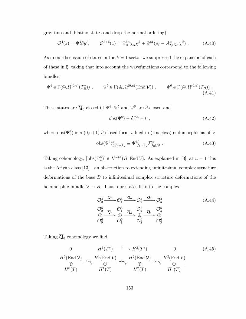
gravitino and dilatino states and drop the normal ordering):
O4pzq “ Ψ4
IByI , O5`6
pzq “ Ψ5αβ χαχ
β`Ψ6I
pρI ´AαIβχαχβq . (A.40)
As in our discussion of states in the k “ 1 sector we suppressed the expansion of each
of these in η; taking that into account the wavefunctions correspond to the following
bundles:
Ψ4P Γp‘uΩ
p0,uqpT ˚Bqq , Ψ5
P Γp‘uΩp0,uq
pEndVqq , Ψ6P Γp‘uΩ
p0,uqpTBqq .
(A.41)
These states are Q0 closed iff Ψ4, Ψ5 and Ψ6 are B-closed and
obspΨ6q ` BΨ5
“ 0 , (A.42)
where obspΨ6uq is a (0,u+1) B-closed form valued in (traceless) endomorphisms of V
obspΨ6qαβJ0¨¨¨Ju
” Ψ6IrJ1¨¨¨Ju
FαJ0sIβ
. (A.43)
Taking cohomology, robspΨ6uqs P H
u`1pB,EndVq. As explained in [3], at u “ 1 this
is the Atiyah class [13]—an obstruction to extending infinitesimal complex structure
deformations of the base B to infinitesimal complex structure deformations of the
holomorphic bundle V Ñ B. Thus, our states fit into the complex
O40
Q0 // O41
Q0 // O42
Q0 // O43
O50
‘
O60
Q0 //O5
1
‘
O61
Q0 //O5
2
‘
O62
Q0 //O5
3
‘
O63
(A.44)
Taking Q0 cohomology we find
0 H1pT ˚q 0 // H2pT ˚q 0
H0pEndVq‘
H0pT q
obs0 //H1pEndVq
‘
H1pT q
obs1 //H2pEndVq
‘
H2pT q
obs2 //H3pEndVq
‘
H3pT q.
(A.45)
153
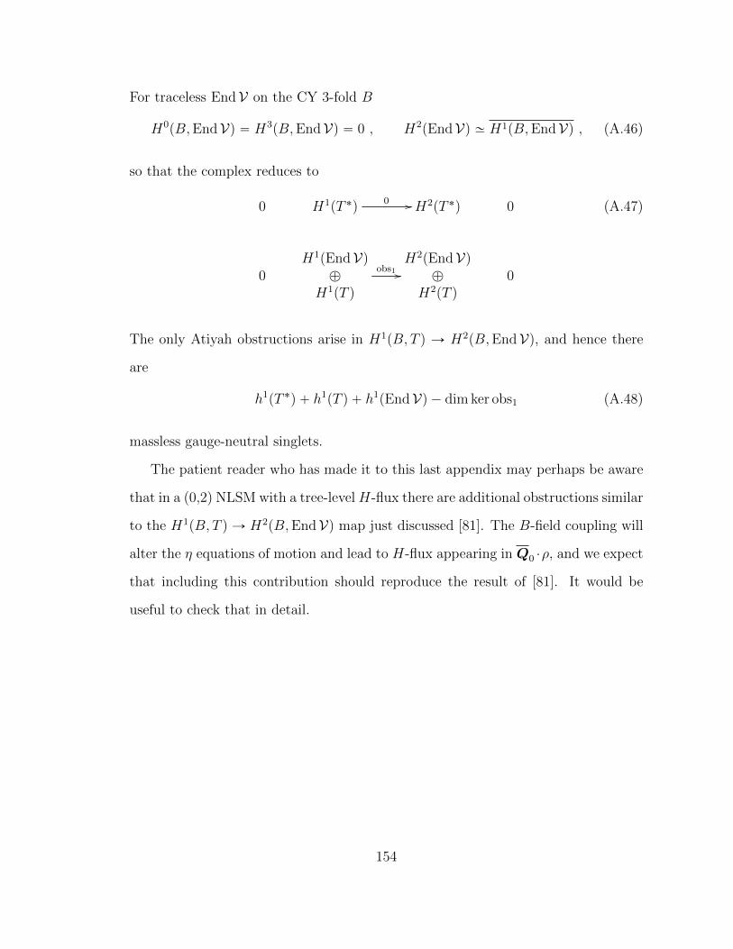
For traceless EndV on the CY 3-fold B
H0pB,EndVq “ H3
pB,EndVq “ 0 , H2pEndVq » H1pB,EndVq , (A.46)
so that the complex reduces to
0 H1pT ˚q0 // H2pT ˚q 0
0H1pEndVq
‘
H1pT q
obs1 //H2pEndVq
‘
H2pT q0
(A.47)
The only Atiyah obstructions arise in H1pB, T q Ñ H2pB,EndVq, and hence there
are
h1pT ˚q ` h1
pT q ` h1pEndVq ´ dim ker obs1 (A.48)
massless gauge-neutral singlets.
The patient reader who has made it to this last appendix may perhaps be aware
that in a (0,2) NLSM with a tree-levelH-flux there are additional obstructions similar
to the H1pB, T q Ñ H2pB,EndVq map just discussed [81]. The B-field coupling will
alter the η equations of motion and lead to H-flux appearing in Q0 ¨ρ, and we expect
that including this contribution should reproduce the result of [81]. It would be
useful to check that in detail.
154
Appendix B
Obstructions to marginal couplings
B.1 An F-term obstruction
In this section we give an example, taken from [11], that illustrates both D-term and
F-term obstructions to marginal couplings. The setting is a (2,2) LG orbifold (LGO)
compactification of the heterotic string with a superpotential
W “ X40 `X
41 `X
42 `X
83 `X
84 ` ψX0X1X2X3X4 ` ε∆W . (B.1)
Here ψ and ε are parameters and ∆W is a generic polynomial with q “ 1. Marginal
(2,0) deformations of the LGO correspond to massless E6-neutral space-time chiral
multiplets. We can compute the massless spectrum exactly as a function of the
complex parameters in the superpotential using the technique developed in [61].
This leads to the following results.
1. Setting ψ “ ε “ 0 leads to a Up1q4 right-moving Kac-Moody algebra and 298
marginal (2,0) deformations. We now turn on the (2,2)-preserving ψ and ε de-
formations and investigate what happens to the remaining (2,0) deformations.
From above we know that at worst the marginal (2,0) deformations can become
marginally irrelevant.
155
2. With ψ ‰ 0 but ε “ 0 the Up1q4 symmetry is broken, and the number of
marginal (2,0) deformations is 298´ 4´ 6 “ 288. While 4 of the 10 marginally
irrelevant deformations are associated to the broken symmetries the 6 others
are not.
3. Finally, turning on ε ‰ 0 does not break any continuous symmetries, but the
number of marginal (2,0) deformations decreases to 288´ 6 “ 282.
Note however, that all the singlets lifted by F-terms correspond to twisted sectors
of the LGO. This is consistent with there being no F-term obstructions in pure LG
theories.
B.2 A D-term obstruction in a heterotic vacuum
Consider now the (2,2) quintic LG theory coupled to a free left-moving fermion with
W “
5ÿ
i“1
ΓiJipΦq “5ÿ
i“1
ΓipΦ4i ` ψ
ź
j‰i
Φjq ` Γ6ˆ 0 . (B.2)
The interacting fields have their usual Up1qL charges qi “ 15 and Qi “ ´45, and
for ψ ‰ 0 there are no extra Up1q symmetries in addition to Up1qL ˆUp1qR ˆUp1q6,
where Up1q6 is the symmetry associated to the free Γ6. This flows to a conformal
field theory with r “ 4 and c “ 9, and we can now consider deformations of the IR
theory from the general perspective of deforming by chiral primary operators. In the
(2,2) theory we have a good understanding of the map between the IR chiral primary
marginal operators and the UV data, so we can identify the marginal deformations
of the IR theory with the space of possible W modulo field redefinitions. If we keep
Γ6 free, we find a 301–dimensional space of deformations.
We can also include deformations of the form Γ6J6, where J6 is some generic
degree 5 polynomial. Although these break the Up1q6 symmetry, they preserve the
central charge and the Up1qL ˆUp1qR quantum numbers of the fields. In particular,
156
Γ6 has the quantum numbers of a free field. Including these J6 deformations yields
a 402-dimensional space of marginal deformations away from the (2,2) r “ 4 c “ 9
fixed point.
Are all of these 402 marginal deformations exactly marginal? While all of the 301
deformations of the Ji are truly marginal, the 101 extra deformations associated to
J6 ‰ 0 are marginally irrelevant. This is completely clear from the conformal pertur-
bation theory discussion we gave in the text. All of these break the Up1q6 symmetry,
and every symmetry-breaking coupling has the same sign of Up1q6 charge. Let us
now see how the same result is recovered from a heterotic space-time perspective.
Heterotic insights
The Z5 orbifold of the LG theory just described, combined with an appropriate
heterotic GSO projection leads to a well-understood heterotic vacuum: the LG point
in the moduli space of the quintic compactification with standard embedding. The
massless fields of the resulting space-time N=1 d “ 4 supergravity theory consist
of the supergravity multiplet, the axio-dilaton chiral multiplet, the e6‘ e8 vector
multiplets, 326 gauge-neutral chiral multiplets, and a e6 charged chiral spectrum
27 ‘ 27‘101
. The 301 deformations of the Ji described above correspond to e6-
preserving marginal deformations in the untwisted sector of the orbifold. These
remain truly marginal for any value of the Kahler modulus (itself in a twisted sector),
and at large radius they are the 101 complex structure deformations of the CY
quintic, as well as 200 of the 224 deformations of the tangent bundle. As reviewed
in [77], there are many arguments for why these deformations are truly marginal.
The 101 deformations associated with the J6 couplings also have a simple space-
time interpretation: they correspond to sop10q-singlet components of the 27‘101
.
Turning on these deformations corresponds to Higgsing e6 Ñ sop10q. This makes it
obvious that the deformations are marginally irrelevant. Under the decomposition
157
of e6 Ą sop10q ‘ up1q, we have
27 “ 16´12 ‘ 101 ‘ 1´2 . (B.3)
The sop10q singlets all have charge ´2 under the broken up1q, and hence have a
D-term space-time potential. This is an example of a “D-term” obstruction to a
marginal coupling being exactly marginal.
Since the deformation only involves world-sheet fields in untwisted sector of the
orbifold, it is clear by the orbifold inheritance principle that this obstruction to
marginality lifts to the un-orbifolded quintic LG model and matches the confor-
mal perturbation theory result. In the orbifold theory it is possible to find exactly
marginal deformations that Higgs e6 Ñ sop10q [34], but they involve an interplay
between marginal couplings in twisted and untwisted sectors [77].
158
Appendix C
GLSMs details
C.1 Linear model conventions
C.1.1 (0,2) superspace
We work in (0,2) superspace1 with coordinate x˘, θ`, θ`
. The supercharges are given
by
Q` “B
Bθ`` iθ
`∇` , Q` “ ´B
Bθ`´ iθ`∇` , (C.1)
where B` “ BBx` and ∇` is the covariant gauge derivative. We also have the
superderivatives
D` “B
Bθ`´ iθ
`∇` , D` “ ´B
Bθ`` iθ`∇` . (C.2)
The non-trivial anti-commutation relations are
tQ`,Q`u “ ´2i∇` , tD`,D`u “ 2i∇` . (C.3)
C.1.2 Field content
There are two types of multiplets in the (0,2) models we consider in this work.
1 More details may be found in [94].
159
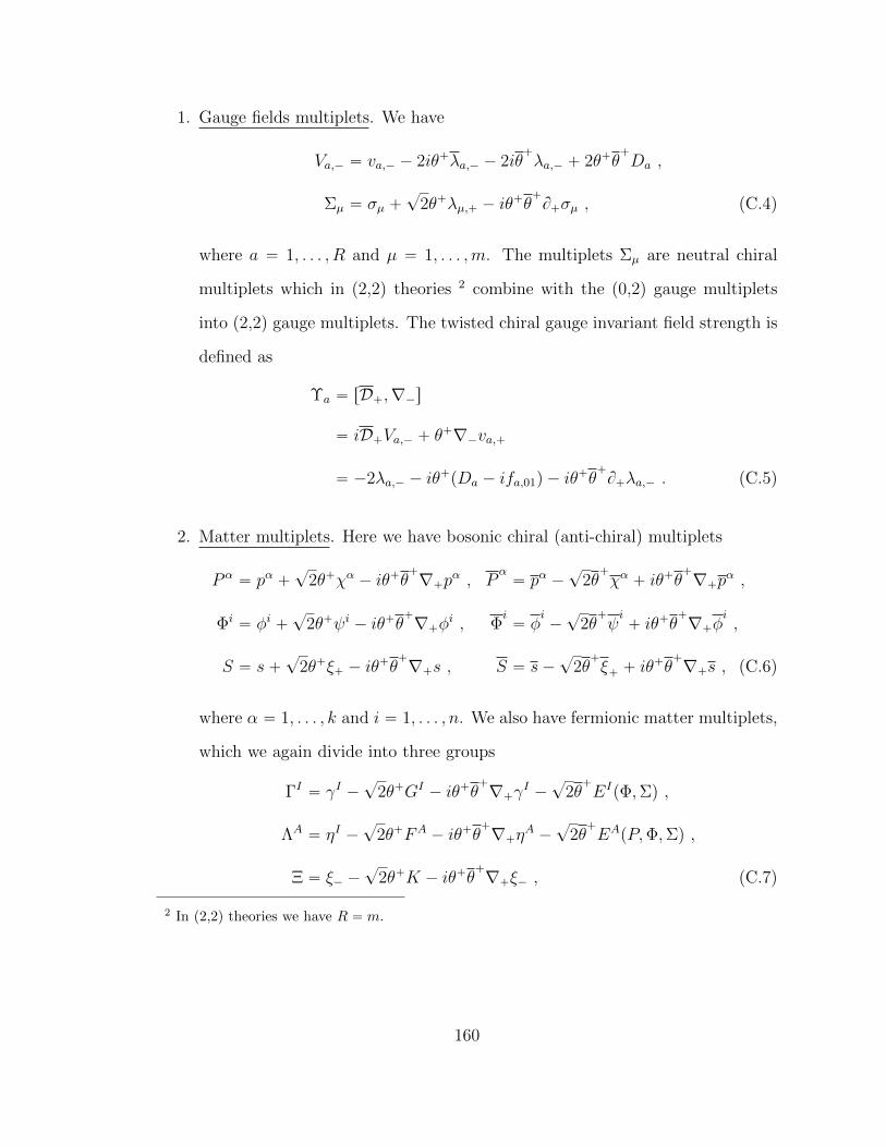
1. Gauge fields multiplets. We have
Va,´ “ va,´ ´ 2iθ`λa,´ ´ 2iθ`λa,´ ` 2θ`θ
`Da ,
Σµ “ σµ `?
2θ`λµ,` ´ iθ`θ`B`σµ , (C.4)
where a “ 1, . . . , R and µ “ 1, . . . ,m. The multiplets Σµ are neutral chiral
multiplets which in (2,2) theories 2 combine with the (0,2) gauge multiplets
into (2,2) gauge multiplets. The twisted chiral gauge invariant field strength is
defined as
Υa “ rD`,∇´s
“ iD`Va,´ ` θ`∇´va,`
“ ´2λa,´ ´ iθ`pDa ´ ifa,01q ´ iθ
`θ`B`λa,´ . (C.5)
2. Matter multiplets. Here we have bosonic chiral (anti-chiral) multiplets
Pα“ pα `
?2θ`χα ´ iθ`θ
`∇`pα , Pα“ pα ´
?2θ`χα ` iθ`θ
`∇`pα ,
Φi“ φi `
?2θ`ψi ´ iθ`θ
`∇`φi , Φi“ φ
i´?
2θ`ψi` iθ`θ
`∇`φi,
S “ s`?
2θ`ξ` ´ iθ`θ`∇`s , S “ s´
?2θ`ξ` ` iθ
`θ`∇`s , (C.6)
where α “ 1, . . . , k and i “ 1, . . . , n. We also have fermionic matter multiplets,
which we again divide into three groups
ΓI “ γI ´?
2θ`GI´ iθ`θ
`∇`γI ´?
2θ`EIpΦ,Σq ,
ΛA“ ηI ´
?2θ`FA
´ iθ`θ`∇`ηA ´
?2θ`EApP,Φ,Σq ,
Ξ “ ξ´ ´?
2θ`K ´ iθ`θ`∇`ξ´ , (C.7)
2 In (2,2) theories we have R “ m.
160
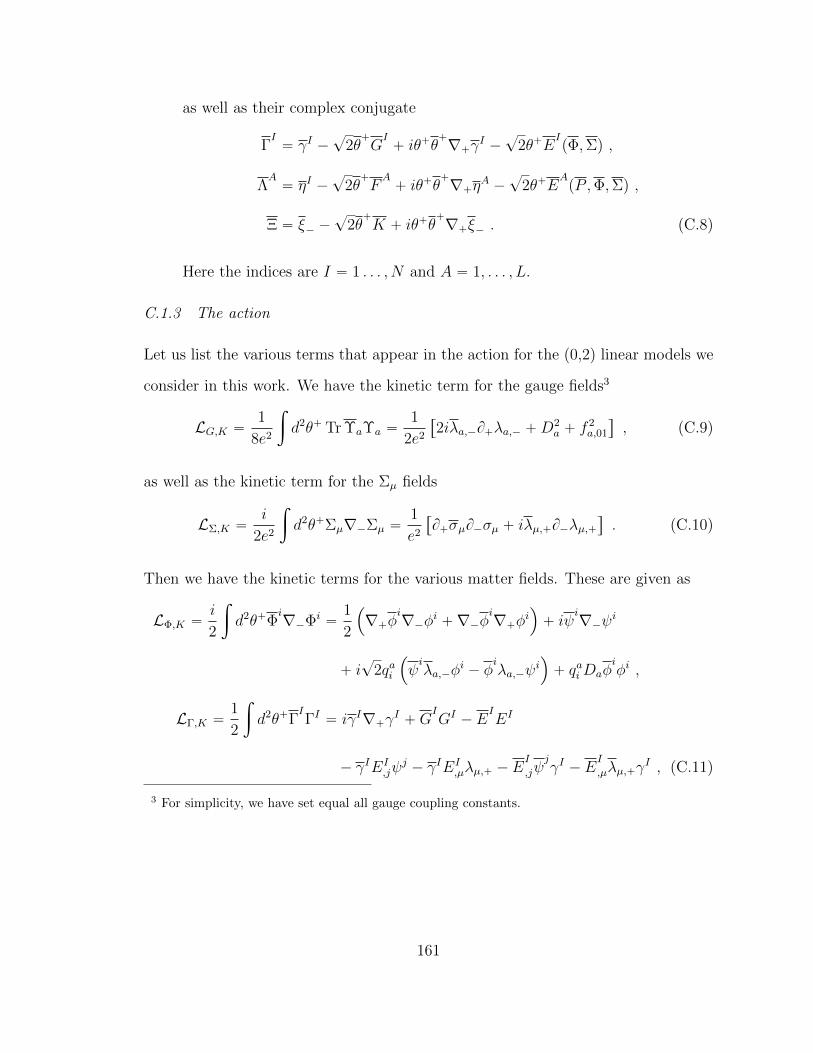
as well as their complex conjugate
ΓI“ γI ´
?2θ`GI` iθ`θ
`∇`γI ´?
2θ`EIpΦ,Σq ,
ΛA“ ηI ´
?2θ`FA` iθ`θ
`∇`ηA ´?
2θ`EApP ,Φ,Σq ,
Ξ “ ξ´ ´?
2θ`K ` iθ`θ
`∇`ξ´ . (C.8)
Here the indices are I “ 1 . . . , N and A “ 1, . . . , L.
C.1.3 The action
Let us list the various terms that appear in the action for the (0,2) linear models we
consider in this work. We have the kinetic term for the gauge fields3
LG,K “1
8e2
ż
d2θ` Tr ΥaΥa “1
2e2
“
2iλa,´B`λa,´ `D2a ` f
2a,01
‰
, (C.9)
as well as the kinetic term for the Σµ fields
LΣ,K “i
2e2
ż
d2θ`Σµ∇´Σµ “1
e2
“
B`σµB´σµ ` iλµ,`B´λµ,`‰
. (C.10)
Then we have the kinetic terms for the various matter fields. These are given as
LΦ,K “i
2
ż
d2θ`Φi∇´Φi
“1
2
´
∇`φi∇´φi `∇´φ
i∇`φi¯
` iψi∇´ψi
` i?
2qai
´
ψiλa,´φ
i´ φ
iλa,´ψ
i¯
` qaiDaφiφi ,
LΓ,K “1
2
ż
d2θ`ΓIΓI “ iγI∇`γI `G
IGI´ E
IEI
´ γIEI,jψ
j´ γIEI
,µλµ,` ´ EI
,jψjγI ´ E
I
,µλµ,`γI , (C.11)
3 For simplicity, we have set equal all gauge coupling constants.
161
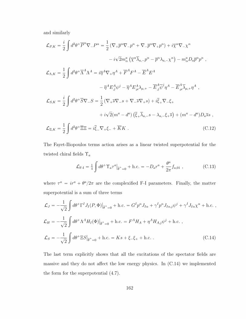
and similarly
LP,K “i
2
ż
d2θ`Pα∇´Pα
“1
2p∇`pα∇´pα `∇´pα∇`pαq ` iχα∇´χα
´ i?
2maα
`
χαλa,´pα´ pαλa,´χ
α˘
´maαDap
αpα ,
LΛ,K “1
2
ż
d2θ`ΛA
ΛA“ iηA∇`ηA ` F
AFA
´ EAEA
´ ηAEA,jψ
j´ ηAEA
,µλµ,` ´ EA
,jψjηA ´ E
A
,µλµ,`ηA ,
LS,K “i
2
ż
d2θ`S∇´S “1
2p∇`s∇´s`∇´s∇`sq ` iξ`∇´ξ`
` i?
2pma´ daq
`
ξ`λa,´s´ λa,´ξ`s˘
` pma´ daqDass ,
LΞ,K “1
2
ż
d2θ`ΞΞ “ iξ´∇`ξ´ `KK . (C.12)
The Fayet-Iliopoulos terms action arises as a linear twisted superpotential for the
twisted chiral fields Υa
LF-I “14
ż
dθ`Υaτaˇ
ˇ
θ`“0` h.c. “ ´Dar
a`θa
2πfa,01 , (C.13)
where τa “ ira ` θa2π are the complexified F-I parameters. Finally, the matter
superpotential is a sum of three terms
LJ “ ´1?
2
ż
dθ`ΓIJIpP,Φqˇ
ˇ
θ`“0` h.c. “ GIpαJIα ` γ
IpαJIα,jψj` γIJIαχ
α` h.c. ,
LH “ ´1?
2
ż
dθ`ΛAHIpΦqˇ
ˇ
θ`“0` h.c. “ FAHA ` η
AHA,jψj` h.c. ,
LS “ ´1?
2
ż
dθ`ΞSˇ
ˇ
θ`“0` h.c. “ Ks` ξ´ξ` ` h.c. . (C.14)
The last term explicitly shows that all the excitations of the spectator fields are
massive and they do not affect the low energy physics. In (C.14) we implemented
the form for the superpotential (4.7).
162
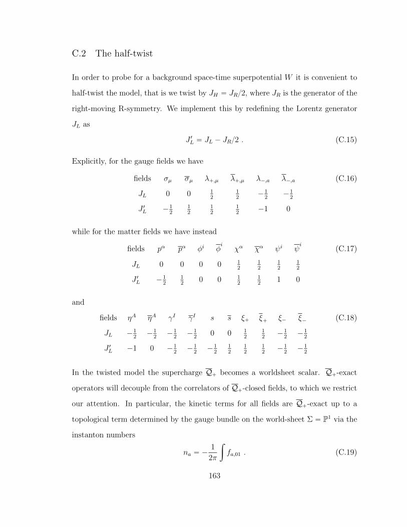
C.2 The half-twist
In order to probe for a background space-time superpotential W it is convenient to
half-twist the model, that is we twist by JH “ JR2, where JR is the generator of the
right-moving R-symmetry. We implement this by redefining the Lorentz generator
JL as
J 1L “ JL ´ JR2 . (C.15)
Explicitly, for the gauge fields we have
fields σµ σµ λ`,µ λ`,µ λ´,a λ´,a
JL 0 0 12
12
´12
´12
J 1L ´12
12
12
12
´1 0
(C.16)
while for the matter fields we have instead
fields pα pα φi φi
χα χα ψi ψi
JL 0 0 0 0 12
12
12
12
J 1L ´12
12
0 0 12
12
1 0
(C.17)
and
fields ηA ηA γI γI s s ξ` ξ` ξ´ ξ´
JL ´12
´12
´12
´12
0 0 12
12
´12
´12
J 1L ´1 0 ´12
´12
´12
12
12
12
´12
´12
(C.18)
In the twisted model the supercharge Q` becomes a worldsheet scalar. Q`-exact
operators will decouple from the correlators of Q`-closed fields, to which we restrict
our attention. In particular, the kinetic terms for all fields are Q`-exact up to a
topological term determined by the gauge bundle on the world-sheet Σ “ P1 via the
instanton numbers
na “ ´1
2π
ż
fa,01 . (C.19)
163
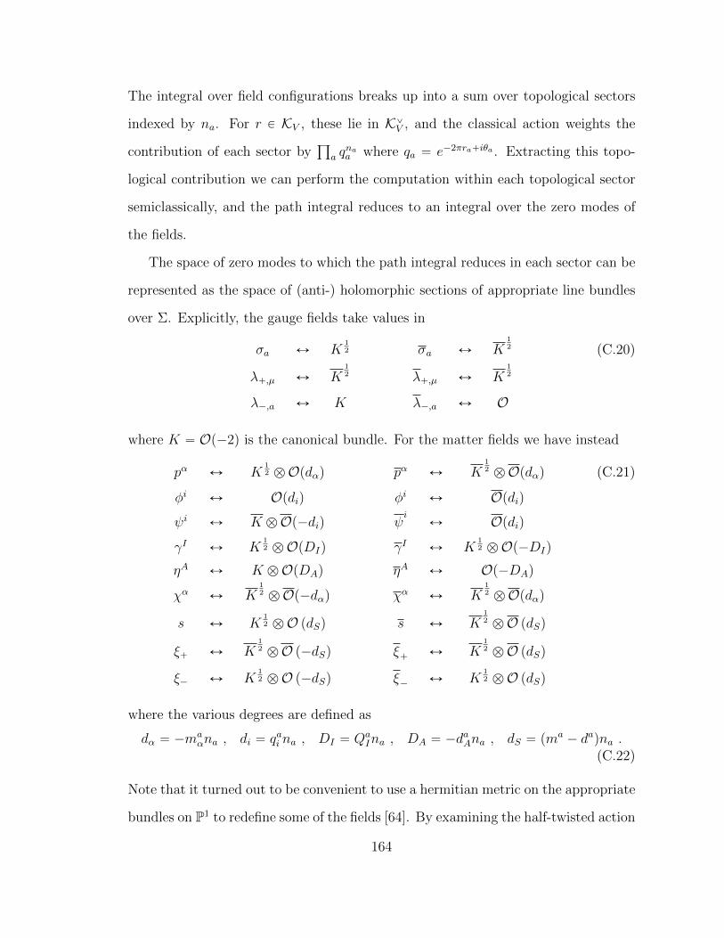
The integral over field configurations breaks up into a sum over topological sectors
indexed by na. For r P KV , these lie in K_V , and the classical action weights the
contribution of each sector byś
a qnaa where qa “ e´2πra`iθa . Extracting this topo-
logical contribution we can perform the computation within each topological sector
semiclassically, and the path integral reduces to an integral over the zero modes of
the fields.
The space of zero modes to which the path integral reduces in each sector can be
represented as the space of (anti-) holomorphic sections of appropriate line bundles
over Σ. Explicitly, the gauge fields take values in
σa Ø K12 σa Ø K
12
λ`,µ Ø K12 λ`,µ Ø K
12
λ´,a Ø K λ´,a Ø O
(C.20)
where K “ Op´2q is the canonical bundle. For the matter fields we have instead
pα Ø K12 bOpdαq pα Ø K
12 bOpdαq
φi Ø Opdiq φi Ø Opdiq
ψi Ø K bOp´diq ψi
Ø Opdiq
γI Ø K12 bOpDIq γI Ø K
12 bOp´DIq
ηA Ø K bOpDAq ηA Ø Op´DAq
χα Ø K12 bOp´dαq χα Ø K
12 bOpdαq
s Ø K12 bO pdSq s Ø K
12 bO pdSq
ξ` Ø K12 bO p´dSq ξ` Ø K
12 bO pdSq
ξ´ Ø K12 bO p´dSq ξ´ Ø K
12 bO pdSq
(C.21)
where the various degrees are defined as
dα “ ´maαna , di “ qai na , DI “ Qa
Ina , DA “ ´daAna , dS “ pm
a´ daqna .
(C.22)
Note that it turned out to be convenient to use a hermitian metric on the appropriate
bundles on P1 to redefine some of the fields [64]. By examining the half-twisted action
164
it is possible to show that the couplings τa as well as H, J and E only appear in
Q`-exact terms. One very important consequence of this for us is that in the half-
twisted theory, correlators of Q`-closed operators are holomorphic in J, H and E,
thus for the purpose of our computations we can set J “ H “ E “ 0.
165
Bibliography
[1] Addington, N. and Aspinwall, P. S. (2013), “Categories of Massless D-Branes anddel Pezzo Surfaces,” .
[2] Addington, N., Segal, E., and Sharpe, E. (2012), “D-brane probes, brancheddouble covers, and noncommutative resolutions,” .
[3] Anderson, L. B., Gray, J., Lukas, A., and Ovrut, B. (2011), “The Atiyah classand complex structure stabilization in heterotic Calabi-Yau compactifications,” .
[4] Aspinwall, P. S. (2011), “A McKay-like correspondence for (0,2)-deformations,”.
[5] Aspinwall, P. S. and Gaines, B. (2014), “Rational Curves and (0,2)-Deformations,” .
[6] Aspinwall, P. S. and Greene, B. R. (1995), “On the geometric interpretation ofN=2 superconformal theories,” Nucl.Phys., B437, 205–230.
[7] Aspinwall, P. S. and Plesser, M. R. (2011), “Elusive worldsheet instantons inheterotic string compactifications,” .
[8] Aspinwall, P. S. and Ronen Plesser, M. (2009), “Decompactifications and Mass-less D-Branes in Hybrid Models,” .
[9] Aspinwall, P. S., Greene, B. R., and Morrison, D. R. (1993), “The monomialdivisor mirror map,” Internat. Math. Res. Notices, pp. 319–337.
[10] Aspinwall, P. S., Greene, B. R., and Morrison, D. R. (1994), “Calabi-Yau modulispace, mirror manifolds and spacetime topology change in string theory,” Nucl.Phys., B416, 414–480.
[11] Aspinwall, P. S., Melnikov, I. V., and Plesser, M. R. (2012), “(0,2) Elephants,”JHEP, 1201, 060.
[12] Atick, J. J., Dixon, L. J., and Sen, A. (1987), “String Calculation of Fayet-Iliopoulos d Terms in Arbitrary Supersymmetric Compactifications,” Nucl.Phys.,B292, 109–149.
166
[13] Atiyah, M. F. (1957), “Complex analytic connections in fibre bundles,” Trans.AMS, 85, 181–207.
[14] Ballmann, W. (2006), Lectures on Kahler manifolds, ESI Lectures in Mathe-matics and Physics, European Mathematical Society (EMS), Zurich.
[15] Banks, T., Dixon, L. J., Friedan, D., and Martinec, E. J. (1988), “Phenomenol-ogy and conformal field theory or can string theory predict the weak mixing angle?”Nucl. Phys., B299, 613–626.
[16] Basu, A. and Sethi, S. (2003), “World-sheet stability of (0,2) linear sigma mod-els,” Phys. Rev., D68, 025003.
[17] Beasley, C. and Witten, E. (2003), “Residues and world-sheet instantons,”JHEP, 10, 065.
[18] Beasley, C. and Witten, E. (2005), “New instanton effects in supersymmetricQCD,” JHEP, 0501, 056.
[19] Becker, K. and Sethi, S. (2009), “Torsional heterotic geometries,” Nucl. Phys.,B820, 1–31.
[20] Becker, K., Becker, M., Fu, J.-X., Tseng, L.-S., and Yau, S.-T. (2006), “Anomalycancellation and smooth non-Kaehler solutions in heterotic string theory,” Nucl.Phys., B751, 108–128.
[21] Behr, N. and Konechny, A. (2014), “Renormalization and redundancy in 2dquantum field theories,” JHEP, 1402, 001.
[22] Belavin, A., Polyakov, A. M., and Zamolodchikov, A. (1984), “Infinite conformalsymmetry in two-dimensional quantum field theory,” Nucl.Phys., B241, 333–380.
[23] Benini, F. and Bobev, N. (2013), “Exact two-dimensional superconformal R-symmetry and c-extremization,” Phys.Rev.Lett., 110, 061601.
[24] Berglund, P., Candelas, P., de la Ossa, X., Derrick, E., Distler, J., et al. (1995),“On the instanton contributions to the masses and couplings of E(6) singlets,”Nucl.Phys., B454, 127–163.
[25] Bertolini, M. and Plesser, M. R. (2015), “Worldsheet instantons and (0,2) linearmodels,” JHEP, 08, 081.
[26] Bertolini, M., Melnikov, I. V., and Plesser, M. R. (2014a), “Accidents in (0,2)Landau-Ginzburg theories,” JHEP, 12, 157.
[27] Bertolini, M., Melnikov, I. V., and Plesser, M. R. (2014b), “Hybrid conformalfield theories,” JHEP, 1405, 043.
167
[28] Blumenhagen, R. and Rahn, T. (2011), “Landscape study of target space dualityof (0,2) heterotic string models,” JHEP, 1109, 098.
[29] Blumenhagen, R., Schimmrigk, R., and Wisskirchen, A. (1996), “The (0,2) Ex-actly Solvable Structure of Chiral Rings, Landau-Ginzburg Theories, and Calabi-Yau Manifolds,” Nucl. Phys., B461, 460–492.
[30] Bott, R. and Tu, L. W. (1982), Differential forms in algebraic topology, vol. 82of Graduate Texts in Mathematics, Springer-Verlag, New York.
[31] Braun, V., Kreuzer, M., Ovrut, B. A., and Scheidegger, E. (2007), “Worldsheetinstantons and torsion curves. Part A: Direct computation,” JHEP, 10, 022.
[32] Calabi, E. (1979), “Metriques kahleriennes et fibres holomorphes,” Ann. Sci.Ecole Norm. Sup. (4), 12, 269–294.
[33] Cox, D. A. and Katz, S. (2000), “Mirror symmetry and algebraic geometry,”Providence, USA: AMS (2000) 469 p.
[34] Dine, M. and Seiberg, N. (1988), “Are (0,2) models string miracles?”Nucl.Phys., B306, 137.
[35] Dine, M., Seiberg, N., Wen, X. G., and Witten, E. (1986), “NonperturbativeEffects on the String World Sheet,” Nucl. Phys., B278, 769.
[36] Dine, M., Ichinose, I., and Seiberg, N. (1987a), “F Terms and d Terms in StringTheory,” Nucl. Phys., B293, 253.
[37] Dine, M., Seiberg, N., Wen, X. G., and Witten, E. (1987b), “NonperturbativeEffects on the String World Sheet. 2,” Nucl. Phys., B289, 319.
[38] Distler, J. (1987), “Resurrecting (2,0) Compactifications,” Phys. Lett., B188,431–436.
[39] Distler, J. (1995), “Notes on (0,2) superconformal field theories,” .
[40] Distler, J. and Greene, B. R. (1988), “Aspects of (2,0) string compactifications,”Nucl. Phys., B304, 1.
[41] Distler, J. and Kachru, S. (1994), “(0,2) Landau-Ginzburg theory,” Nucl. Phys.,B413, 213–243.
[42] Dixon, L. J. (1987), “Some world sheet properties of superstring compactifi-cations, on orbifolds and otherwise,” Lectures given at the 1987 ICTP SummerWorkshop in High Energy Physics and Cosmology, Trieste, Italy, Jun 29 - Aug 7,1987.
168
[43] Dixon, L. J., Friedan, D., Martinec, E. J., and Shenker, S. H. (1987), “TheConformal Field Theory of Orbifolds,” Nucl. Phys., B282, 13–73.
[44] Donagi, R. and Wijnholt, M. (2009), “Higgs bundles and UV completion inF-theory,” .
[45] Donagi, R., Lu, Z., and Melnikov, I. V. (2014), “Global aspects of (0,2) modulispace: toric varieties and tangent bundles,” .
[46] Eguchi, T., Gilkey, P. B., and Hanson, A. J. (1980), “Gravitation, gauge theoriesand differential geometry,” Phys.Rept., 66, 213.
[47] El-Showk, S., Paulos, M. F., Poland, D., Rychkov, S., Simmons-Duffin, D., et al.(2012), “Solving the 3D Ising Model with the Conformal Bootstrap,” Phys.Rev.,D86, 025022.
[48] El-Showk, S., Paulos, M. F., Poland, D., Rychkov, S., Simmons-Duffin, D.,et al. (2014), “Solving the 3d Ising Model with the Conformal Bootstrap II. c-Minimization and Precise Critical Exponents,” .
[49] Erkal, D. and Kutasov, D. (2010), “a-Maximization, Global Symmetries andRG Flows,” .
[50] Freedman, D. and Gibbons, G. (1981), “Remarks on supersymmetry and Kahlergeometry,” in Superspace and supergravity, eds. S. Hawking and M. Rocek, Cam-bridge University Press.
[51] Gepner, D. (1987), “Exactly solvable string compactifications on manifolds ofSU(N) holonomy,” Phys.Lett., B199, 380–388.
[52] Green, D., Komargodski, Z., Seiberg, N., Tachikawa, Y., and Wecht, B. (2010),“Exactly marginal deformations and global symmetries,” JHEP, 1006, 106.
[53] Greene, B. R. and Plesser, M. R. (1990), “Duality in Calabi-Yau moduli space,”Nucl. Phys., B338, 15–37.
[54] Griffiths, P. and Harris, J. (1978), Principles of algebraic geometry, Wiley-Interscience [John Wiley & Sons], New York, Pure and Applied Mathematics.
[55] Higashijima, K., Kimura, T., and Nitta, M. (2003), “Construction of supersym-metric nonlinear sigma models on noncompact Calabi-Yau manifolds with isome-try,” Nucl.Phys.Proc.Suppl., 117, 867–869.
[56] Hori, K., Katz, S., Klemm, A., Pandharipande, R., Thomas, R., Vafa, C., Vakil,R., and Zaslow, E. (2003), Mirror symmetry, vol. 1 of Clay Mathematics Mono-graphs, American Mathematical Society, Providence, RI, With a preface by Vafa.
169
[57] Hull, C. M. and Witten, E. (1985), “Supersymmetric sigma models and theheterotic string,” Phys. Lett., B160, 398–402.
[58] Intriligator, K. A. and Vafa, C. (1990), “Landau-Ginzburg Orbifolds,”Nucl.Phys., B339, 95–120.
[59] Intriligator, K. A. and Wecht, B. (2003), “The exact superconformal R-symmetry maximizes a,” Nucl. Phys., B667, 183–200.
[60] Joyce, D. D. (2000), Compact manifolds with special holonomy, Oxford Mathe-matical Monographs, Oxford University Press, Oxford.
[61] Kachru, S. and Witten, E. (1993), “Computing the complete massless spectrumof a Landau- Ginzburg orbifold,” Nucl. Phys., B407, 637–666.
[62] Kapustin, A. and Li, Y. (2003), “Topological correlators in Landau-Ginzburgmodels with boundaries,” Adv. Theor. Math. Phys., 7, 727–749.
[63] Kastor, D. A., Martinec, E. J., and Shenker, S. H. (1989), “RG Flow in N=1Discrete Series,” Nucl. Phys., B316, 590–608.
[64] Katz, S. H. and Sharpe, E. (2006), “Notes on certain (0,2) correlation functions,”Commun. Math. Phys., 262, 611–644.
[65] Kawai, T. and Mohri, K. (1994), “Geometry of (0,2) Landau-Ginzburg orb-ifolds,” Nucl. Phys., B425, 191–216.
[66] Kawai, T., Yamada, Y., and Yang, S.-K. (1994), “Elliptic genera and N=2superconformal field theory,” Nucl.Phys., B414, 191–212.
[67] Klemm, A. and Schimmrigk, R. (1994), “Landau-Ginzburg string vacua,”Nucl.Phys., B411, 559–583.
[68] Kreuzer, M. and Skarke, H. (1992a), “No mirror symmetry in Landau-Ginzburgspectra!” Nucl.Phys., B388, 113–130.
[69] Kreuzer, M. and Skarke, H. (1992b), “On the classification of quasihomogeneousfunctions,” Commun.Math.Phys., 150, 137.
[70] Kreuzer, M., McOrist, J., Melnikov, I. V., and Plesser, M. (2011), “(0,2) defor-mations of linear sigma models,” JHEP, 1107, 044.
[71] Kutasov, D. (2003), “New results on the ’a theorem’ in four-dimensional super-symmetric field theory,” .
[72] Kutasov, D. and Schwimmer, A. (2004), “Lagrange multipliers and couplings insupersymmetric field theory,” Nucl.Phys., B702, 369–379.
170
[73] Lazarsfeld, R. (2004), Positivity in algebraic geometry. I, vol. 48 of A Series ofModern Surveys in Mathematics, Springer-Verlag, Berlin.
[74] Lindstrom, U., Rocek, M., von Unge, R., and Zabzine, M. (2007), “GeneralizedKahler manifolds and off-shell supersymmetry,” Commun.Math.Phys., 269, 833–849.
[75] Martinec, E. J. (1989), “Algebraic Geometry and Effective Lagrangians,” Phys.Lett., B217, 431.
[76] McOrist, J. and Melnikov, I. V. (2009), “Summing the instantons in half-twistedlinear sigma models,” JHEP, 02, 026.
[77] McOrist, J. and Melnikov, I. V. (2012), “Old issues and linear sigma models,”Adv.Theor.Math.Phys., 16, 251–288.
[78] Melnikov, I., Sethi, S., and Sharpe, E. (2012a), “Recent Developments in (0,2)Mirror Symmetry,” SIGMA, 8, 068.
[79] Melnikov, I. V. (2009), “(0,2) Landau-Ginzburg models and residues,” JHEP,09, 118.
[80] Melnikov, I. V. and Plesser, M. R. (2011), “A (0,2) mirror map,” JHEP, 1102,001.
[81] Melnikov, I. V. and Sharpe, E. (2011), “On marginal deformations of (0,2) non-linear sigma models,” Phys.Lett., B705, 529–534.
[82] Melnikov, I. V., Minasian, R., and Theisen, S. (2012b), “Heterotic flux back-grounds and their IIA duals,” .
[83] Moroianu, A. (2007), Lectures on Kahler geometry, vol. 69, Cambridge Univer-sity Press, Cambridge.
[84] Morrison, D. R. and Ronen Plesser, M. (1995), “Summing the instantons: quan-tum cohomology and mirror symmetry in toric varieties,” Nucl. Phys., B440, 279–354.
[85] Nekrasov, N. A. (2005), “Lectures on curved beta-gamma systems, pure spinors,and anomalies,” .
[86] Periwal, V. and Strominger, A. (1990), “Kahler geometry of the space of N=2superconformal field theories,” Phys.Lett., B235, 261.
[87] Polchinski, J. (1988), “Scale and conformal Invariance in quantum field theory,”Nucl.Phys., B303, 226.
171
[88] Polchinski, J. (2007), String theory. Vol. 1: An introduction to the bosonic string,Cambridge University Press.
[89] Seiberg, N. (1995), “Electric - magnetic duality in supersymmetric nonAbeliangauge theories,” Nucl. Phys., B435, 129–146.
[90] Silverstein, E. and Witten, E. (1994), “Global U(1) R symmetry and conformalinvariance of (0,2) models,” Phys. Lett., B328, 307–311.
[91] Silverstein, E. and Witten, E. (1995), “Criteria for conformal invariance of (0,2)models,” Nucl. Phys., B444, 161–190.
[92] Vafa, C. (1989), “String Vacua and Orbifoldized L-G Models,” Mod. Phys. Lett.,A4, 1169.
[93] Vafa, C. and Warner, N. P. (1989), “Catastrophes and the Classification ofConformal Theories,” Phys. Lett., B218, 51.
[94] Wess, J. and Bagger, J. (1992), Supersymmetry and supergravity, PrincetonUniversity Press.
[95] West, P. (1990), Introduction to supersymmetry and supergravity, World Scien-tific, Singapore.
[96] Witten, E. (1986), “New Issues in Manifolds of SU(3) Holonomy,” Nucl. Phys.,B268, 79.
[97] Witten, E. (1993), “Phases of N = 2 theories in two dimensions,” Nucl. Phys.,B403, 159–222.
[98] Witten, E. (1994), “On the Landau-Ginzburg description of N=2 minimal mod-els,” Int. J. Mod. Phys., A9, 4783–4800.
[99] Witten, E. (2005), “Two-dimensional models with (0,2) supersymmetry: Per-turbative aspects,” .
[100] Zamolodchikov, A. (1986), “Conformal symmetry and multicritical points intwo-dimensional quantum field theory. (In Russian),” Sov.J.Nucl.Phys., 44, 529–533.
172
Biography
My name is Marco Bertolini, and I was born in Reggio Emilia, Italy, on June 25,
1985. I completed my high school degree at Liceo Scientifico Aldo Moro in Reggio
Emilia. I earned a BS in Physics from Universita degli Studi di Parma under the
supervision of Professor Roberto De Pietri. In the same department, I obtained a MS
in Theoretical Physics under the supervision of Dott. Luca Griguolo. Then, I joined
the graduate program at Duke University where I have been studying string theory
for the past five years under the supervision of Professor Ronen Plesser. My passion
for the subject will bring me to Japan, where I will hold a postdoctoral position at
Kavli IPMU.
173