Chapter two: Behavior of Centrifugal Pumps in Operation

Chap te r | two

Behaviorof Centrifugal

Pumps in Operation2.1 CHARACTERISTICS OF CENTRIFUGAL PUMPS

The characteristic curves indicate the behavior of a pump under chang-

ing operating conditions (Fig. 2.1). The head H, power input P and effi-

ciency h at constant speed n are plotted against the flow rateQ (Fig. 2.2).Figure 2.3 shows the head-capacity curves (Q–H curves) at various

speeds and the iso-efficiency curves.

Dependent on the specific speed, the slope of the head characteristicvaries from flat (low specific speed) to steep (high specific speed); see

Fig. 2.4.

Radial impellers cover the specific speed range up to about nq = 120(NSUSA = 6200).

Mixed-flow impellers are feasible from nq = 40 to about nq = 200

(NSUSA = 2000�10 000).Axial-flow impellers with very steep (but often unstable) characteris-

tics are built with specific speeds nq = 160 to about nq = 350

(NSUSA = 8000 to 18 000) (see Fig. 2.1).A head-capacity curve of a centrifugal pump is said to be stablewhen

the head curve rises steadily from high flow towards shut-off, i.e. there is

always a negative slope dH/dQ. For any given head there is a uniqueintersection with the Q–H curve. Pumps with low specific speeds are

prone to flat Q–H curves or even a slight instability. Axial-flow pumps

(high specific speed) usually have a flow range with a distinct instability,within which it is not permissible to operate (see Fig. 2.1).

On radial pumps, stable characteristics can be obtained by the

following measures:. small impeller outlet angle;. extended return vanes on multistage pumps;. relatively large impeller outlet width;. small number of vanes.

27

Centrifugal Pump Handbook. DOI: 10.1016/B978-0-7506-8612-9.00002-4

Figure 2.5 shows an unstable characteristic, the Q–H curves beingintersected twice by the pump characteristic when, for example, the grid

frequency drops. The pump may revert to minimum or zero flow with a

risk of overheating because the power input to the pump is then con-verted into heat.

Pumps with unstable characteristics may interact with the system in

closed circuits, leading to flow oscillations (surge) and possibly pipevibrations. Stable characteristics are a fundamental requirement for

the automatic control of centrifugal pumps.

2.2 CONTROL OF CENTRIFUGAL PUMPS

2.2.1 Piping system characteristic

The head to be overcome consists of a static component Hgeo which is

independent of the flow rate, and a head loss Hdyn increasing with thesquare of the flow and depending on pipework layout, pipe diameter

and length. The sum HA = Hgeo + Hdyn represents the head required by

the system at any given flow rate. The resulting curve HA = f(Q) is termedthe ‘‘system curve’’ (Fig. 2.6). Centrifugal pumps adjust themselves auto-

matically to the intersection of the system and head characteristics. The

operating point is given by the intersection of the Q–H curve with thesystem characteristic.

In many applications the static head is zero, and the system head is

entirely due to hydraulic losses.

2.2.2 Pump control

Pump output may be controlled by the following methods:

1. Throttling

Figure 2.1 Typical shapes of the characteristics of centrifugal pumps

28 Behavior of Centrifugal Pumps in Operation

2. Switching pumps on or offa. with pumps operating in parallel

b. or with pumps operating in series

3. Bypass control4. Speed control

Figure 2.2 Typical pump characteristics with various impeller diametersand constant speed

Control of Centrifugal Pumps 29

5. Impeller vane adjustment6. Pre-rotation control

7. Cavitation control.

2.2.2.1 THROTTLINGClosing a throttle valve in the discharge line increases the flow resistance

in the system. The system characteristic becomes steeper and intersects

the pump characteristic at a lower flow rate. To avoid a reduction of theNPSHA, throttling is not admissible in the suction pipe.

Figure 2.3 Typical pumpcharacteristics for constant impeller diameter andvariable speed


Throttling control (Fig. 2.7) is generally employed where the requiredflow rate deviates from the nominal flow for short periods of operation.

The power input P0 in kWh per m3 liquid pumped increases with

falling flow rate:

P0 ¼ r � H

367 � hkWh

m3

� �¼ const:

H

h

r in kg=dm3

H in m

i.e. P0 depends only on the ratio H/h.

Figure 2.4 Influence of specific speed on the shape of the characteristics


This reasoning demonstrates that throttling control ought to be employ-ed mainly on radial pumps with nq � �40 (NSUSA � 2000), because these

have a flatter H-to-Q characteristic and are better suited for such control.

With high specific speeds (nq > 100, NSUSA > 5000) this control iswasteful of energy because the power input to the pump rises when

throttling is effected. Even the driver may be overloaded that way. More-

over, the flow conditions in the pump deteriorate at low flow rates,causing uneven running.

2.2.2.2 STARTING AND STOPPING PUMPSParallel operationWhere the pumping requirement varies, it may be desirable to employ

several small pumps instead of a few large units. When the required flow

Figure 2.5 Influence of an unstable characteristic on the operatingbehavior of a pump under frequency variation

Figure 2.6 System characteristic


rate drops, one ormore pumps are stopped. The remainder then operatecloser to their best efficiency point.

With a given suction head and flow rate, a greater number of

pumps may sometimes yield benefits because higher pump speedcan then be adopted enabling pump costs to be lowered. The opti-

mum number of pumps must be chosen in the light of the constraints

of the system (space requirements, costs of auxiliary equipment anderection).

Parallel operation is conditional upon a steadily rising pump head

curve.With Hgeo � Hdyn, operating pumps in series is not advisable

(Fig. 2.8a). If one pump shuts down, consideration must be given to

how far the remaining pump can run out to the right and whether theNPSH available covers the NPSH required (Fig. 2.8).

At the same time the driver power must be sufficient to ensure pump

runout with adequate margin.Positive displacement pumps can also be run in parallel with centri-

fugal pumps. A positive displacement pump has an H–Q characteristic

which is almost vertical. Here again Q values for the same head areadded, giving the combined characteristic plotted in Fig. 2.9. The inter-

section of the system head curvewith the combined pump characteristic

is the duty point. By combining centrifugal and positive displacementpumps, one disadvantage of the latter (no throttle control) can be com-

pensated partially.

Figure 2.7 Throttling control and power input at constant rpm


Figure 2.8 Series and parallel operation

Figure 2.9 Reciprocating and centrifugal pumps operating in parallel


Series operationWhen flow-dependent losses are dominating, i.e. Hgeo � Hdyn, pumpsmay be operated in series. The reason for this will be clear from Fig. 2.8c.

With predominantly dynamic losses, series operation is advisable

because it is still possible to deliver about 70% of the original flow ifone of 2 pumps is shut down. Moreover the pump operates with better

NPSH and good efficiency.

If, however, Hgeo � Hdyn (i.e. a mainly static system) series operationis not recommended. When one pump fails in series operation, the other

runs at lower flow and lower efficiency in a range where uneven perfor-

mance must be expected (Fig. 2.8a). In this case, pumps in paralleloperate much better and give greater flow at a higher efficiency.

Where pumps operate in series, it must be borne in mind that the

seals and casings on the downstream pump are under higher pressure.The shaft seal may have to be balanced to the suction pressure of the

upstream pump. Recirculation losses result from this, which must be

taken into account in the overall efficiency calculation.

2.2.2.3 BYPASS CONTROLIn order to vary flow, centrifugal pumps are sometimes controlled by

means of a bypass, i.e. a certain capacity is piped back to the suction

nozzle or – if large capacities are involved – to a vessel at the suction end(see also section 2.8: Minimum flow rate). The pump then operates to the

right of its optimum point (depending on the system head curve), and its

cavitation behavior must be reviewed. Owing to recirculation losses, theoverall efficiency drops markedly.

This method is used only rarely to control centrifugal pumps, and

judged by the criterion of overall efficiency, it is the least satisfactorysystem compared to speed control and throttling (Figs 2.10, 2.11 and

2.12). Bypass control is, however, employedmore often with pumpswith

Figure 2.10 Typical bypass control system


high specific speed, such as axial-flow pumps, because the power inputdrops with increasing flow.

2.2.2.4 SPEED CONTROLWhere the head required by the plant is made up wholly or mainly from

hydraulic losses, speed control is best, because pump efficiency thenremains practically constant. Though speed control is expensive, wear

on the pump and valves is less, so that the lifespan of both is generally

Figure 2.11 Various control systems with steep system head curve


increased. Furthermore, operating costs are reduced, because higherpump efficiency means less power input (Figs 2.11 and 2.12).

Unlike throttling, speed control leaves the piping system character-

istic unchanged, while the pump characteristic moves up or down inaccordance with the speed change. Two or more pumps serving a com-

mon discharge line are usually installed.

Speed control is achieved by employing the following drivingmachinery:. steam turbines

Figure 2.12 Various control systems with flat system head curve


. diesel engines

. pole-reversing electric motors

. variable-speed electric motors (slip-ring motors, frequency-controlled

or thyristor-controlled motors). electromagnetic couplings. hydraulic couplings. hydrostatic couplings. variable-speed gears.

When varying speed, the following equations hold good in accor-

dance with the law of similarity:

Q1

Q2¼ n1

n2

H1

H2¼ n1

n2

� �2 NPSH1

NPSH2¼ n1

n2

� �2

From the last of these equations it is clear that increasing the speedincreases the NPSHreq as well. A higher NPSHav must be provided.

Moreover, increasing speed increases power input approximately by

the third power of the speed. Consequently the strength of the shaftmust always be verified before increasing the speed. With small speed

changes (up to 10%) efficiency remains virtually unchanged.

With larger speed changes the velocity in the channels alters andwith it the Reynolds number. The efficiency factor must be downgraded

at lower speeds and upgraded at higher ones (see section 3.2.4: Con-

version of test results).

2.2.2.5 IMPELLER BLADE ADJUSTMENTFor axial pumps (and even semi-axial pumps of high specific speed)

impellers with adjustable blades can provide a most economical control

for duties involving a widely varying flow rate. If the demanded flow rateincreases, the impeller blade angles are increased by turning the blades

around an axis essentially perpendicular to the hub.

Figure 2.13 shows a family of characteristics for various blade set-tings with the setting angle b as parameter at a constant speed. The

higher the head, the greater is the cavitation coefficient and therefore

the required NPSH. At low flow rates the characteristics of axial pumpsare usually unstable; operation in this range must be avoided.

Impeller blade adjustment is used on water circulating pumps. Withconstant water level, these pumps can be controlled economically on the

system characteristic.

2.2.2.6 PRE-ROTATION CONTROL

For pre-rotation control, the impeller is preceded by controllable inlet

guide vanes. The pump characteristic is altered solely by varying inflowto the impeller. The setting of the pre-rotation guide imparts a circum-

ferential component to the inflowing medium, thus altering the energy

conversion process in the pump and with it the characteristic.


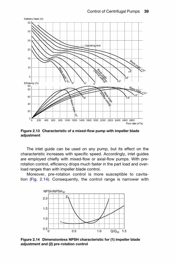
The inlet guide can be used on any pump, but its effect on thecharacteristic increases with specific speed. Accordingly, inlet guides

are employed chiefly with mixed-flow or axial-flow pumps. With pre-

rotation control, efficiency drops much faster in the part load and over-load ranges than with impeller blade control.

Moreover, pre-rotation control is more susceptible to cavita-

tion (Fig. 2.14). Consequently, the control range is narrower with

Figure 2.13 Characteristic of a mixed-flow pump with impeller bladeadjustment

Figure 2.14 Dimensionless NPSH characteristic for (1) impeller bladeadjustment and (2) pre-rotation control


this method than with impeller blade adjustment. Depending on

the shape of the system head curve, the head can be controlleddown to about 70 to 50% of its value at the best efficiency point

(Fig. 2.15).

Figure 2.15 Characteristics of a mixed-flow water circulating pump withpre-rotation control


2.2.2.7 CAVITATION CONTROLCavitation control is often used to vary the flow rate on smaller conden-sate pumps. The head per stage is generally limited to 50 m, otherwise

the pump will run too unevenly and sustain excessive cavitation wear on

the vanes. If condensate flow in the hotwell is below operating flow, thelevel will drop and with it the available NPSH, and the pump cavitates.

The break-off characteristic now intersects elsewhere with the systemhead curve, at a lower flow rate.

If the flow of condensate into the hotwell increases above the

momentary flow rate of the pump, the liquid level rises, and with it theavailable NPSH. This alters the cavitation status, and pump flow

increases (Fig. 2.16). The intersection of variable NPSHav with pump

NPSHreq at full cavitation determines the flow rate. Simplicity is theargument for this control system.

2.3 MATCHING CHARACTERISTICSTO SERVICE DATA

2.3.1 Reduction of impeller diameter (impeller trimming)

If the flow required by the system is permanently less than the pump

flow at best efficiency point, and speed control is not applicable, theimpeller can be matched to the new conditions by reducing its diam-

eter (see Fig. 2.17). On diffuser pumps, only the impeller blades are

cut (Fig. 2.17b), while on volute casing pumps, usually the impellerblades with the shrouds are turned down (Fig. 2.17a and e).

With diffuser or double-entry pumps, it is often advisable to trim the

impeller obliquely as in Fig. 2.17c or d, because such corrections usuallyyield a more stable curve.

The bigger the correction is and the higher the specific speed, the

more the pump efficiency suffers from adaptation.

Figure 2.16 Cavitation control

Matching Characteristics to Service Data 41

Bigger corrections increase pump NPSH in the overload range,because specific vane loading is raised by the reduced vane length,

affecting velocity distribution at the impeller inlet.

If only a small correction (�5%) to impeller outside diameter isnecessary, it may be assumed that the required NPSH will increase

only slightly.

When pump impeller diameters are reduced, outlet width, bladeangle and blade length are altered. The effect of this depends very

much on the design of the impeller (i.e. on its specific speed). Con-

sequently, only approximate statements can be made about theeffects of reducing the impeller diameter on characteristics.

Figure 2.17 Impeller corrections


When radial impellers are corrected, the pump characteristic altersaccording to Fig. 2.18 as follows:

Q0 ¼ Q

D0

D

!m

H0 ¼ H

D0

D

!m

wherem = 2 to 3 may be assumed:m = 2 for corrections�6%;m = 3 for

corrections �1%It should be noted that the best efficiency point lies betweenQ0 andQ,

depending on nq.

In accordance with Fig. 2.18, operating point B is joined to pointQ = 0, H = 0 by a straight line. The new operating point is found by

plotting Q0 on the Q axis or H0 on the H axis. In this way the corrected

impeller diameter can be determined.If an impeller with higher specific speed (nq > 50,NSUSA > 2500) is to

bematched, or the correction amounts tomore than 3%, thematching to

service data should be effected in stages, i.e. first turning-down to alarger diameter than the one calculated and carrying out a trial run. Only

after this is the impeller corrected to its final diameter.

2.3.2 Sharpening of impeller blade trailing edges

By sharpening the impeller blades on the suction side (also called under-

filing), the outlet angle can be enlarged to obtain up to 5% more headnear the best efficiency point, depending on the outlet angle. At least

2 mm must be left (Fig. 2.19). In this way efficiency can be improved

slightly (Fig. 2.20).Where stage pressures are high, underfiling must be carried out with

great care on account of the high static and dynamic stresses involved.

Figure 2.18 Alteration of the pump characteristic after reduction of theimpeller diameter

Matching Characteristics to Service Data 43

2.4 TORQUE/SPEED CURVES

2.4.1 Starting torque of centrifugal pumps

Normally, the centrifugal pump starting torque is so low that it does notrequire special consideration. Drivers like steam, gas and water turbines

have very high driving torques. The difference between driver and pump

torque is sufficient to accelerate a centrifugal pump to its operatingspeed in a very short time.

Figure 2.19 Sharpening of impeller blades

Figure 2.20 Influence of sharpening of impeller blades on pumpcharacteristic


Where a pump is driven by an internal combustion engine, the starter

must be sufficiently large to bring both the engine and pump up tooperating speed. However, a clutch is usually interposed to separate

the pump from the engine during startup.

Depending upon their type and size, electric motors have varioustorque characteristics (see section 7.1.4). With high power inputs in

particular, startup must therefore be investigated thoroughly at the plan-

ning stage. At around 80% of the speed the torque of an electric motormay drop to the pump torque. Acceleration torque is then nil, and the

group becomes locked into this speed. As a result, the motor takes up a

high current, with the risk of destroying the windings (Fig. 2.21). Pumptorque T is calculated as follows:

T ¼ 9549 ðP=nÞ ðNmÞP ¼ pump power input ðkWÞ n ¼ rpm

In accordance with the affinity law, the torque varies as the square of

the speed:

T2 ¼ T1ðn2=n1Þ2

To achieve initial pump breakaway, a starting torque between 10 and

25% of pump torque at best efficiency point is normally required

Figure 2.21 Starting torque curve for electric motor and pump

Torque/Speed Curves 45

because of the static friction of the moving parts involved. For vertical

pumps with long rising mains or pumps with very high inlet pressures,initial breakaway torque must be calculated specially (number of bear-

ings, thrust bearing friction, stuffing box friction, etc.).

The torque curve depends very much on specific speed, as may beseen from Fig. 2.4. Pumps with lower specific speed have a torque

characteristic that rises with flow rate, whereas pumps with high specific

speed have a characteristic that falls, as flow increases.

2.4.2 Startup (excluding pressure surge)

Centrifugal pumps may be started in four different ways.

2.4.2.1 STARTUP AGAINST CLOSED VALVEFigure 2.22 plots the startup of a centrifugal pump against a closed valve.

With comparatively high ratings, the pump must start with a minimumflow valve opened, due to the risk that liquid will evaporate inside the

pump. As soon as operating speed is reached, the discharge valve is

opened. This method is possible only on pumps with low specific speed,where the power input and torque with closed valve are less than at the

duty point.

2.4.2.2 STARTUP AGAINST CLOSED NON-RETURN VALVE WITH THEDISCHARGE VALVE OPEN (FIG. 2.23)

When starting, the non-return valve opens at point A, when the back

pressure acting on it is reached. As the speed increases, flow rate and

head follow the system curve.

2.4.2.3 STARTUP WITH DISCHARGE VALVE OPEN BUT NO STATIC HEAD (FIG. 2.24)Here, the torque curve is a parabola through duty point B, provided that

the pipe is short and that the time needed to accelerate the water columncoincides with the pump startup time.

Figure 2.22 Starting against closed valve


2.4.2.4 STARTUP WITH DISCHARGE VALVE OPEN AND PRESSUREPIPELINE DRAINED (FIG. 2.25)

Pumps with high specific speed are mostly started with the pipeline

drained. A backpressure ought to be established as quickly as possible,

if necessary by throttling with the discharge valve, to prevent high pumprunout flows where there is danger of cavitation.

Figure 2.23 Startup against closed non-return valve with discharge valveopen

Figure 2.24 Startup with discharge valve open but no geodetic head

Figure 2.25 Startup with discharge valve open and pressure pipelinedrained

Torque/Speed Curves 47

Starting up pumps of this type with the pressure pipeline filled

is also possible, provided considerable quantities are diverted via abypass.

2.5 STARTUP TIME FOR A CENTRIFUGAL PUMP

The startup time for a centrifugal pump depends on the acceleratingtorque, i.e. on the difference between the torque of the driving unit TAand the starting torque Tp required by the pump.

The accelerating torque varies with the speed (Fig. 2.26). The startuptime must therefore be calculated for individual speed increments and

then totaled:

TB ¼ TA � Tp ¼ Je ðNmÞ

where J = mass moment of inertia for all revolving parts including liquid,

related to driving speed:

J ¼ mD2

4ðkg m2Þ

where D = inertia diameter:

J2 � J1ðn1=n2Þ2 ðkgm2Þ

Figure 2.26 Calculating the startup time for a centrifugal pump


e ¼ dv=dt ¼ p

30� dndt

¼ angular acceleration of drive shaft1

s2

� �

From the above equations, startup time is calculated as follows:

tA ¼ Sti ¼ p � J30

Dn1TB1

þ Dn2TB2

þ . . . :þ DniTBi

� �ðsÞ

where J ðkgm2Þ n ðmin�1Þ TB ðNmÞ .Depending on whether the pump starts with the discharge valve

open or closed, its starting torque (Tp) and hence its startup time will

also vary.

2.6 RUNDOWN TIME FOR A CENTRIFUGALPUMP (DISREGARDING THEPRESSURE SURGE)

When the driving unit is shut down or fails, the drive torque drops to zero.

The following then holds good:

�Tp ¼ Je ðNmÞ

Tp ¼ runout torque ¼ pump starting torque ðNmÞ

J ¼ mass moment of inertia for all revolving parts related to

drive speed ðpump including liquidÞ

e ¼ dv=dt ¼ p

30� dndt

¼ angular acceleration of drive shaft1

s2

� �

From the above equations, the runout time is calculated asfollows:

tH ¼ Sti ¼ p � J30

Dn1TP1

þ Dn2TP2

þ . . . :þ DniTPi

� �ðsÞ

with J ðkgm2Þ n ðmin�1Þ Tp ðNmÞ .Depending on whether the pump is shut down with the discharge

valve open or closed, its runout torque (Tp) varies and hence its runout

time also.

Because the value Dn1/TP1 is very small immediately after shutdown,the speed drops very rapidly at first (Fig. 2.27). However, the effective

rundown time is obtained from the pressure surge calculation (see

section 4.3).

Rundown Time for A Centrifugal Pump 49

2.7 PUMPING SPECIAL LIQUIDS

2.7.1 Viscous liquids

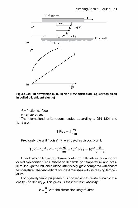
2.7.1.1 VISCOSITY DEFINITIONSIf a plate ismoved at constant speed co over a viscousmedium (Fig. 2.28),

the medium adheres to the underside of the plate and is entrained at the

speed co. The internal friction of the liquid causes the speed to vary atright angles to the direction of flow between the fixed and moving plates:

F ¼ hA � dc=dyrelated to the friction surface of the underside:

t ¼ h dc=dy

The proportionality factor h is called dynamic viscosity, with the

dimension mass/(length � time):

F ¼ h � A � dcdy

!t ¼ hdc

dy

where:

F = frictional force

h = dynamic viscosity

Figure 2.27 Runout time for a condensate pump


A = friction surfacet = shear stress

The international units recommended according to DIN 1301 and

1342 are:

1 Ps s ¼ 1kg

s m

Previously the unit ‘‘poise’’ (P) was used as viscosity unit:

1 cP ¼ 10�2 � P ¼ 10�3 kg

ms¼ 10�3 Pa s ¼ 10�2 g

cm � sLiquids whose frictional behavior conforms to the above equation are

called Newtonian fluids. Viscosity depends on temperature and pres-

sure, though the influence of the latter is negligible compared with that of

temperature. The viscosity of liquids diminishes with increasing temper-ature.

For hydrodynamic purposes it is convenient to relate dynamic vis-

cosity h to density r. This gives us the kinematic viscosity:

v ¼ h

rwith the dimension length2=time

Figure 2.28 (I) Newtonian fluid. (II) Non-Newtonian fluid (e.g. carbon blackin boiled oil, effluent sludge)

Pumping Special Liquids 51

The following units are introduced by DIN 1301 and 1342:

1mm2

s¼ 10�6 m2

s

Previously the unit ‘‘stoke’’ (St) was customary:

1 cSt ¼ 10�2 St ¼ mm2

s¼ 10�6 m2

s

Besides the official units set out above, other conventional units are inuse for kinematic viscosity:

1. Degrees Engler (E): The degree Engler expresses the ratio between

the efflux time of 200 cm3 distilled water at 20�C and of the sameamount of test liquid at 20�C (DIN 51560). The following equation is

used for conversion:

v ¼� E � 7:6 1�1=�E3ð Þ 10�6 �m2

s

� �

2. Saybolt viscosity: Saybolt seconds universal (SSU). This unit is

customary in the USA and defines the efflux time for a given quan-tity of liquid from a defined viscosity meter.

Viscosity also depends to a considerable extent on the amount of

gas dissolved in the liquid. Crude oil containing a lot of gas is less viscousthan the same oil with little gas.

2.7.1.2 PUMPING VISCOUS LIQUIDSBy virtue of their favorable properties (little pulsation, no safety valve

needed as with positive displacement pumps, simple flow control)the use of centrifugal pumps is being increasingly extended in the

chemical industry and refineries to high-viscosity media (up to about

1000 � 10�6 m2/s), although an efficiency loss must be taken into accountcompared with positive displacement pumpswith the same service data.

The economical application limit for centrifugal pumps is about (150

to 500) 10�6 m2/s; this limit very much depends on the pump size andapplication. The use of a centrifugal pump is possible up to about

1500 � 10�6 m2/s and even above. Tests are available with viscosities

up to 3000 � 10�6 m2/s. Reciprocating or rotary positive displacementpumps are employed for still higher viscosities (Fig. 2.29).

Due to increased losses, higher NPSH must be made available when

pumping liquids with viscosities appreciably higher than cold water.The pressure losses in the impeller and diffuser channels of centrif-

ugal pumps, the impeller friction and internal leakage losses, depend to alarge extent on the viscosity of the pumped liquid. Consequently, the

characteristics ascertained for water lose their validity when pumping

liquids of higher viscosity, such as oil.


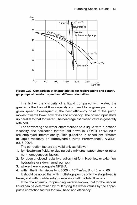
The higher the viscosity of a liquid compared with water, thegreater is the loss of flow capacity and head for a given pump at a

given speed. Consequently, the best efficiency point of the pump

moves towards lower flow rates and efficiency. The power input shiftsup parallel to that for water. The head against closed valve is generally

retained.

For converting the water characteristic to a liquid with a definedviscosity, the correction factors laid down in ISO/TR 17766 2005

are employed internationally. This guideline is based on: ‘‘Effects

of Liquid Viscosity on Rotodynamic Pump Performance’’, ANSI/HI9.6.7-2004.

The correction factors are valid only as follows:

1. for Newtonian fluids, excluding solid mixtures, paper stock or othernon-homogeneous liquids;

2. for open or closed radial hydraulics (not for mixed-flow or axial-flow

hydraulics or side-channel pumps);3. where there is adequate NPSHA;

4. within the limits: viscosity < 3000 � 10�6 m2/s; B < 40; nq < 60.

It should be noted that with multistage pumps only the stage head istaken, and with double-entry pumps only half the total flow rate.

If the characteristic for pumping water is known, that for the viscous

liquid can be determined by multiplying the water values by the appro-priate correction factors for flow, head and efficiency.

Figure 2.29 Comparison of characteristics for reciprocating and centrifu-gal pumps at constant speed and different viscosities


2.7.1.3 SIMPLIFIED INSTRUCTIONS FOR DETERMINING PUMP PERFORMANCEON A VISCOUS LIQUID WHEN PERFORMANCE ON WATER IS KNOWN

The following equations and charts are used for developing the cor-

rection factors to adjust pump water performance characteristics of rateof flow, total head, efficiency, and input power to the corresponding

viscous liquid performance.

Step 1Calculate parameter B based on the water performance best efficiency

flow (QBEP–W).Given metric units QBEP–W in m3/h, HBEP–W in m, N in rpm and Vvis in

cSt, use the following equation:

B ¼ 16:5� ðVvisÞ0:50 � ðHBEP�WÞ0:0625ðQBEP�WÞ0:375 � N0:25

Given USCS units ofQBEP–W in gpm, HBEP–W in ft, N in rpm and Vvis incSt, use the following equation:

B ¼ 26:6� ðVvisÞ0:50 � ðHBEP�WÞ0:0625ðQBEP�WÞ0:375 � N0:25

If 1.0 < B < 40, go to Step 2.

If B � 40, the correction factors derived using the equations aboveare highly uncertain and should be avoided. Instead a detailed loss

analysis method may be warranted.

If B � 1.0, set CH = 1.0 and CQ = 1.0, and then skip to Step 4.

Step 2Read the correction factor for flow (CQ) (which is also equal to thecorrection factor for head at BEP [CBEP–H]) corresponding to the water

performance best efficiency flow (QBEP–W) using the chart in Fig. 2.30.

Correct the other water performance flows (QW) to viscous flows (Qvis).

Step 3Read the head correction factors (CH) using the chart in Fig. 2.30, andthen the corresponding values of viscous head (Hvis) for flows (QW)

greater than or less than the water best efficiency flow (QBEP–W).

Step 4Determine the value for Ch from the chart in Fig. 2.31.

Step 5Calculate the values for viscous pump shaft input power (Pvis). The

following equations are valid for all rates of flow greater than zero.For flow in m3/h, head in m, shaft power in kW, and efficiency in

percent, use the equation below:

PvisQvis � Hvis�tot � s

367� hvis


For flow in gpm, head in ft, and shaft power in hp, use the equationbelow:

PvisQvis � Hvis�tot � s

3960� hvis

where s = specific gravity.

Figure 2.30 Chart of correction factors for CQ and CH based on flow andhead correction factors versus parameter B

Figure 2.31 Chart of correction factors for Ch based on the efficiency cor-rection factor versus parameter B


2.7.2 Gas/liquid mixtures

Air or gas may enter a centrifugal pump due to air-entraining vortices,

poor sealing of the inlet pipes or chemical processes.However, a centrifugal pump can handle liquids containing air or

gas only to a very limited extent. Self-priming pumps are exceptions.

Dissolved air or gas is separated from the liquid upon reduction of

Figure 2.32 Influence of air on the characteristic of a single-stage centri-fugal pump (nq = 26) with inlet pressure 2.5 bar absolute


the local pressure (Henry’s law). The air or gas can gather at the

impeller inlet or anywhere in the flow passages. When these are suffi-ciently blocked by gas accumulations the flow may collapse.

Figure 2.32 shows the influence of air on the characteristics of a

single-stage centrifugal pump with specific speed nq = 26 (NSUSA =1350). This influence depends on the suction pressure. Here, with

low inlet pressure, the characteristic already drops at VL/Q00 = 2%

(volume percentage at inlet pressure 2.5 bar absolute), especially at highand low flow rates. As the air content rises, head, flow rate, efficiency and

power input decline. The pump cannot be operated down to closed

discharge valve. If there is more than 5 to 7% gas, the flow may collapsealtogether even at best efficiency point.

For multistage pumps, the gas content limit is determined by the first

stage. Susceptibility to air influence is, however, less with regard to theshape of the characteristic, since at each subsequent stage, the gas

bubbles pass on to a higher pressure level and thus exert volume-wise

less influence on the characteristic.With increasing air content theNPSHrequired also increases as shown in Fig. 2.33.

Figure 2.33 Influence of air content on NPSH (Q = constant, n = constant)


2.7.3 Pumping hydrocarbons

2.7.3.1 INFLUENCE ON SUCTION CAPACITY (NPSH)The required NPSH for centrifugal pumps is normally determined only for

handling clean, cold water. Nevertheless, test and accumulated experi-ence have shown that pumps can handle hydrocarbons with less NPSH

than would be necessary for cold water.

The expected NPSH reduction is a function of vapor pressure andthe density of the hydrocarbons to be pumped. Figure 2.34 shows

schematically the loss of head for cold, degassed water and for a

defined hydrocarbon. With cold water, a much greater volume of vaporforms at the impeller entry at a given NPSH. This obstruction re-

duces the head. As the NPSH is reduced further, the growing vapor

volume causes an abrupt loss of head. With hydrocarbons, there is lessvolume of vapor at low NPSH, so that the loss of head is delayed and

more gradual.

Figure 2.35 depicts maximum admissible NPSH reductions for hotdegassed water and certain gas-free hydrocarbons (according to the

Hydraulic Institute). The NPSH reductions shown are based on operating

experience and experimental data.The validity of the diagram is subject to the following limitations:

1. The reduction may not exceed 50% of the NPSH necessary for cold

water, or a maximum of 3 m, whichever is smaller.2. It applies only to low-viscosity liquids and hydrocarbons free of air

and gas.3. It does not apply to transient operating conditions.

4. It applies when pumping petroleum products (mixtures of different

hydrocarbons), provided the vapor pressure of the mixture is deter-mined for the light fractions.

Figure 2.34 Loss of head with two different liquids


2.7.4 Handling solid–liquid mixtures with centrifugalpumps

By virtue of their simple design, uniform delivery, good ratio between

delivery and size and low susceptibility to trouble, centrifugal pumps arealso employed for handlingmixtures of liquids and granular solids (termed

‘‘slurries’’). For higher flow rates centrifugal pumps are also less expensive

than positive displacement pumps for comparable pumping data.A large variety of goods, including coal, iron ore, fly ash, gravel, sewage,

fish, sugarbeet, potatoes,woodpulp,paper stockandsuspensionsof lime,

can be handled by centrifugal pumps. More details are given in Chapter 9under the headings of solid-conveyance pumps, sewage pumps, pumps

for the paper industry and pumps for flue gas desulphurization plants.

Figure 2.35 Maximum admissible NPSH reduction for hot, degassed waterand certain gas-free hydrocarbons (Hydraulic Institute, 14th edition, 1983)


Attention should be drawn to the following special features:

1. Such pumps should be operated under ample NPSHA.2. The impeller channels and volute cross-sectionsmust be large enough

to allow passage of the biggest solid particles expected. Back shroud

blades must keep abrasive particles away from the stuffing box.3. Flow velocity through the impeller and volute must be kept low to

minimize abrasion, which increases with the third power of the

velocity. The heads of these centrifugal pumps are presently limitedto about 80 m. Admissible pipeline velocity depends on the density,

particle size, form and concentration of the solids involved.

4. Flow velocity through pipelines may not drop below critical settlingvelocity, otherwise the solids will be precipitated from the suspen-

sion. The minimum flow velocity must be at least 0.3 m/s above the

critical settling velocity (Fig. 2.37).5. The centrifugal pump should have a steep characteristic. If the

concentration of solids is changed, the resistance curve alters

too. If the characteristic is steep, pump delivery will then drop onlyslightly and flow velocity variation in the lines is also only slight (Fig.

2.36). Segregation of the solids is thus prevented.

6. Slurry pumps are often operated in series in order to meet thedemand for a steep characteristic.

7. When the pipeline is partly blocked by solids which have settled

upon shutdown, the pump must generate sufficient flow to get thesolids moving. The higher resistances encountered at startup must

be overcome, so that adequate flow velocity may be achieved to

resume transportation process.8. When pumping long fibers, open impellers should be used on

account of the clogging risk. The inlet edges should be profiled

and thickened so that fibers can slide off them more easily.9. Slurry pumps are subject to heavy wear. This is reflected in losses of

head, flow rate and efficiency, andmust be taken into account when

sizing the system, drivers and pumps.

Figure 2.36 Segregation of solids as a function of flow velocity at constantmixture ratio m


10. The pump materials must be selected judiciously for the liquid andsolids involved. Depending on its abrasiveness and/or corro-

siveness, rubber, plastic or enamel linings can be provided, or alter-

natively particularly hard materials must be used.Table 2.1 compares the Tyler screen sizes and mesh sizes in mm.

Table 2.2 shows the settling velocities for various solids as a function of

solid particle size.

Table 2.1 Comparison of Screen Sizes: Tyler and Mesh (mm)

Tyler standard sieve series Grade

Mesh width Mesh

inch mm

Theoreticalvalues

3

Screen

shingle

gravel

2

1.5

1.050 26.67

0.883 22.43

0.742 18.85

0.624 15.85

0.525 13.33

0.441 11.20

0.371 9.423

(Continued)

Figure 2.37 Pipeline characteristic as a function of solids concentrationand particle size


Table 2.1 Comparison of Screen Sizes: Tyler and Mesh (mm) (continued)


Mesh width Mesh

inch mm

Theoreticalvalues

0321 7.925 2.5

0263 6.68 3

0.221 5.613 3.5

0.185 4.699 4

0.156 3.962 5

0.131 3.327 6

0.110 2.794 7

0.093 2.362 8

Very

coarse

sand

0.078 1.981 9

0.065 1.651 10

0.055 1.397 12

0.046 1.168 14

0.039 0.991 16

Coarse

sand

0.0328 0.833 20

0.0276 0.701 24

0.0232 0.589 28

0.0195 0.495 32

Medium

sand

0.0164 0.417 35

0.0138 0.351 42

0.0116 0.295 48

0.0097 0.248 60

Fine

sand

0.0082 0.204 65

0.0069 0.175 80

0.0058 0.147 100

0.0049 0.124 115

0.0041 0.104 150

0.0035 0.089 170

0.0029 0.074 200

Silt0.0024 0.061 250

0.0021 0.053 270

(Continued)


Table 2.1 Comparison of Screen Sizes: Tyler and Mesh (mm) (continued)


Mesh width Mesh

inch mm

Theoreticalvalues

0.0017 0.043 325

0.0015 0.038 400

0.025 500

0.020 625

0.010 1250

0.005 2500

0.001 12500

Table 2.2 Sinking Velocities for Various Abrasive Materials

Soilgrain sizeidentification

Diameterin mm

Meshsize USfine

Sinkingvelocityin m/s

ASTM US Bureau ofSoils USDA

MIT Interna-tional

0.0002 0.00000003 Clay Clay Medium-

coarse clay

Fine clay

0.0006 0.00000028 Coarse clay Coarse clay

0.001 0.0000070

0.002 0.0000092 Fine silt Fine silt

0.005 0.0017 Silt Silt Medium-

coarse silt

Coarse silt

0.006 0.000025

0.02 0.00028 Coarse silt

0.05 270 0.0017 Fine

sand

Very fine

sand0.06 230 0.0025

0.10 150 0.070 Fine sand Fine sand Fine sand

0.20 70 0.021

0.25 60 0.026Coarse

sand

Sand Medium-

coarse sand

Medium-

coarse sand0.30 0.032

0.50 35 0.053Coarse sand Coarse sand

0.60 30 0.063

1.00 18 0.10Fine gravel Coarse sand Very coarse

sand2.00 10 0.17


2.8 MINIMUM FLOW RATE

Minimum flow rate is the lowest pump delivery that can be maintainedfor extended periods of operation without excessive wear or even

damage. Minimum flow should be distinguished from minimum

continuous flow which represents the lower limit of the preferableoperation range, where the pump is allowed to operate for an inde-

terminate time.

Minimum flow rate of centrifugal pumps is determined by the follow-ing criteria:. temperature rise due to the internal energy loss;. increased vibration due to excessive flow separation and recirculation;. increased pressure fluctuation at part load;. increased axial thrust at low flow rates;. increased radial thrust (especially with single-volute pumps).

2.8.1 Determining the minimum flow rate

2.8.1.1 ADMISSIBLE TEMPERATURE RISECentrifugal pumps convert only part of their power input into hydraulic

energy. Some of it is converted into heat energy by friction. This internalenergy loss depends very much on the flow rate through the pump, as is

shown in Fig. 2.38. The external energy losses due to bearing and stuffingbox friction are small and are ignored here. The lower the flow rate, the

lower the efficiency and hence the greater the internal energy loss

Figure 2.38 Effective energy and energy losses of a centrifugal pump


converted into heat. The temperature of the water in the pumps risesasymptotically with diminishing flow (Fig. 2.39). To avoid overheating and

possible evaporation in the pump, a certain amount of liquid (the so-

called thermal minimum flow) passes through the pump.

Figure 2.39 Temperature rise of the liquid in a pump and admissibleminimum flow rate

Minimum Flow Rate 65

The temperature rise in the pump is calculated for incompressible

flow as:

DtD ¼ 0:00981

c� H � 1

hi

� 1

� �in �C

H ¼ total head in m hi ¼ h=hm ¼ internal efficiency

c in kJ=kg � Khm ¼ mechanical efficiency

for water: c = 4.18 kJ/kg � KA temperature rise results from throttling an incompressible liquid in

the clearance of the axial thrust balancing device:

DtD ¼ 0:00981

c� DHhi

The total temperature rise including the balancing system must betaken into account when determining minimum flow, especially where

liquids are pumped close to their vaporization pressure.

More accurate calculations are advisable for compressible flows atvery high pressures (>2000 m).

With multistage pumps, the pressure behind the balancing piston or

disc must always be sufficiently far removed from the vapor pressurecorresponding to the calculated temperature.

For smaller pumps running at a temperature sufficiently far from that

corresponding to the vapor pressure, it will suffice to determineminimumflow by means of the following formula:

Qmin ¼ PðkWÞ � 3600r

kg

m3

� �� c kJ

kg � K� �

� tE � tsð Þm3

h

� �

The admissible temperature rise tE – tS is given by the existing tem-

perature tS at the suction nozzle and the admissible temperature tEbehind the balancing device. About 20�C may be taken as temperature

difference. With small pumps, the balancing flow may be adequate as

minimum flow. In such cases the Qmin calculated from the above equa-tion must be equal to or less than the balancing flow. If the calculated

Qmin exceeds the balancing flow, at least the difference between the two

must be passed through a minimum flow bypass.Thisminimum flow on small pumpsmay take the form of a continuous

flow with a throttling device (with the disadvantage of reduced overall

pump efficiency), or of flow controlled by means of an automatic recir-culation control valve or a flow meter.

Theminimum flow rate is either returned directly to the suction nozzle

(but only if the available NPSH of the pump is well above required NPSH)or into the inlet tank. The latter arrangement is recommended, because


the warmed water then mixes with the colder water in the tank. This is

particularly advisable for hot water pumps, where the temperature rise atthe impeller entry may cause a substantial loss of NPSHavail.

2.8.1.2 POOR HYDRAULIC BEHAVIOR IN THE PART LOAD RANGEThe temperature rise discussed above is not the only criterion for deter-

mining minimum flow. For small pumps (up to about 100 kW), the min-imum flow calculated by means of the above formula is sufficient. For

pumps with a power input above about 1000 kW and with high specific

speed, however, the forces due to flow recirculation at the impeller entrymay, even at 25 to 35% of the best efficiency point flow rate, be so great

that excessive vibration is excited in the pump and pipework. Higher

minimum flow rates are necessary for such pump sizes (Fig. 2.40).

Figure 2.40 Minimum flow rate guidelines as a function of specific speedand pump type for power inputs exceeding 1000 kW

Minimum Flow Rate 67

Special attentionmust be given to impellers with large eye diameters.

Though they have a better NPSHfull cavitation, the NPSH0% increases rap-idly at part load. With such impellers, reverse flow at the entry already

begins at around 40 to 60% of best point flow (Fig. 2.40).

2.8.1.3 INFLUENCE OF AXIAL AND RADIAL THRUSTThe increasing axial thrust that occurs as flow diminishes in pumpsoperating at minimum flow for extended periods of time must be accom-

modated by suitable bearings. Single-volute pumps set up high radial

thrusts under part loads, calling for appropriate precautions such asreinforcing the shaft and bearings.


Documents

Chapter two: Behavior of Centrifugal Pumps in Operation