Chapter 9: Measuring and managing interest rate risks Chapter objectives . . . . . . . . . . . . . . . . . . . . . . . . . . . . . . . . . . . . . . . . . . . . . . . . . . . . . . . 1Section 9.1. Debt service and interest rate risks . . . . . . . . . . . . . . . . . . . . . . . . . . . . . . . . 2

Section 9.1.1. Optimal floating and fixed rate debt mix . . . . . . . . . . . . . . . . . . . . 3Section 9.1.2. Hedging debt service with the Eurodollar futures contract . . . . . . . 4Section 9.1.3. Forward rate agreements . . . . . . . . . . . . . . . . . . . . . . . . . . . . . . . . 10

Section 9.2. The interest rate exposure of cash flow and earnings for financial institutions. . . . . . . . . . . . . . . . . . . . . . . . . . . . . . . . . . . . . . . . . . . . . . . . . . . . . . . . . . . . . . . 11

Section 9.3. Measuring and hedging interest rate exposures . . . . . . . . . . . . . . . . . . . . . 19Section 9.3.1. Measuring yield exposure . . . . . . . . . . . . . . . . . . . . . . . . . . . . . . 20Section 9.3.2. Improving on traditional duration . . . . . . . . . . . . . . . . . . . . . . . . 28

Section 9.3.2.A. Taking into account the slope of the term structure incomputing duration . . . . . . . . . . . . . . . . . . . . . . . . . . . . . . . . . . . 28

Section 9.3.2.B. Taking into account convexity . . . . . . . . . . . . . . . . . . . 32Section 9.3.2.C. “Maturity bins” to protect against changes in the slope and

shape of the term structure . . . . . . . . . . . . . . . . . . . . . . . . . . . . . . 37Section 9.4. Measuring and managing interest rate risk without duration . . . . . . . . . . . . 38

Section 9.4.1. Using zero coupon bond prices as risk factors . . . . . . . . . . . . . . . 41Section 9.4.2. Reducing the number of sources of risk: Factor models . . . . . . . 43Section 9.4.3. Forward curve models . . . . . . . . . . . . . . . . . . . . . . . . . . . . . . . . . 45

Section 9.5. Summary . . . . . . . . . . . . . . . . . . . . . . . . . . . . . . . . . . . . . . . . . . . . . . . . . . . 50Key concepts . . . . . . . . . . . . . . . . . . . . . . . . . . . . . . . . . . . . . . . . . . . . . . . . . . . . . . . . . . 51Review questions . . . . . . . . . . . . . . . . . . . . . . . . . . . . . . . . . . . . . . . . . . . . . . . . . . . . . . . 52Questions and exercises . . . . . . . . . . . . . . . . . . . . . . . . . . . . . . . . . . . . . . . . . . . . . . . . . . 53Technical Box 9.1. The tailing factor with the Euro-dollar futures contract . . . . . . . . . . 55Technical Box 9.2. Orange County and VaR . . . . . . . . . . . . . . . . . . . . . . . . . . . . . . . . . . 57Technical Box 9.3. Riskmetrics™ and bond prices . . . . . . . . . . . . . . . . . . . . . . . . . . . . . 59Table Box 9.1. Riskmetrics™ mapping of cash flows . . . . . . . . . . . . . . . . . . . . . . . . . . 60Table 9.1. Eurodollar futures prices. . . . . . . . . . . . . . . . . . . . . . . . . . . . . . . . . . . . . . . . . 62Table 9.2. Interest Rate Sensitivity Table for Chase Manhattan . . . . . . . . . . . . . . . . . . . 64Table 9.3. Example from Litterman and Scheinkman (1991). . . . . . . . . . . . . . . . . . . . . . 65Figure 9.1. Example of a Federal Reserve monetary policy tightening. . . . . . . . . . . . . . 66Figure 9.2. Bond price as a function of yield . . . . . . . . . . . . . . . . . . . . . . . . . . . . . . . . . . 67Figure 9.3. The mistake made using delta exposure or duration for large yield changes. 68Figure 9.4. Value of hedged bank. . . . . . . . . . . . . . . . . . . . . . . . . . . . . . . . . . . . . . . . . . 69Figure 9.5.Term Structures . . . . . . . . . . . . . . . . . . . . . . . . . . . . . . . . . . . . . . . . . . . . . . . 70Literature note . . . . . . . . . . . . . . . . . . . . . . . . . . . . . . . . . . . . . . . . . . . . . . . . . . . . . . . . . 71

Chapter 9: Measuring and managing interest rate risks

September 21, 2001

© René M. Stulz 1998, 2000, 2001

Chapter 9, page 1

Chapter objectives

At the end of this chapter, you will:

1. Understand the tradeoff between fixed and floating rate debt.

2. Be able to measure interest rate exposures.

3. Have tools to measure interest rate risks with VaR and CaR.

4. Understand how interest rate models can be used to hedge and measure interest rate risks.

Chapter 9, page 2

In 1994, interest rate increases caused a loss of $1.6 billion for Orange County, California,

ultimately leading the county to declare bankruptcy. If Orange County had measured risk properly,

this loss would most likely never have happened. In this chapter, we introduce tools to measure and

hedge interest rate risks. We show how Orange County could have used these tools. Much of our

analysis deals with how interest rate changes affect the value of bond portfolios, but we also discuss

how financial institutions as well as non-financial corporations can hedge interest rate risks associated

with their funding. Firms can alter their interest rate risks by changing the mix of fixed and floating

rate debt they have. We investigate the determinants of the optimal mix of floating and fixed rate debt

for a firm and show how a firm can use a futures contract to switch from floating rate debt to fixed

rate debt.

Financial institutions are naturally sensitive to interest rate risks. We therefore examine how

financial institutions measure and manage their exposure to interest rate changes and explain why

these institutions care about this exposure. Interest rate risks affect a firm’s cash flow as well as its

value. The techniques to measure and manage the cash flow impact and the value impact of interest

rate changes differ and are generally used by different types of institutions.

Duration is a popular approach to measure interest rate risk. We show how duration is

computed, how it is used, when it is appropriate, and how one can improve on duration. We also

present approaches to measure interest rate risk that do not rely on duration. We explain how to

estimate VaR for simple fixed income securities with and without duration.

Section 9.1. Debt service and interest rate risks

There is generally an optimal mix of floating-rate and fixed rate debt for a firm at a particular

Chapter 9, page 3

time. A Eurodollar futures contract is one instrument to hedge the interest rate risks of floating-rate

debt. An alternative financial instrument is a forward rate agreement.

Section 9.1.1. Optimal floating and fixed rate debt mix

A firm’s choice of funding is part of its risk management strategy. Non-callable fixed rate debt

has a fixed coupon payment. The debt service does not make cash flows volatile because there is no

uncertainty about payments that have to be made to service the debt. Floating rate debt has interest

rate payments tied to an index, generally an interest rate - for instance, the U.S. prime rate. The

variability of the debt service may heighten or reduce the volatility of cash flows.

A firm whose business produces revenues that are higher when interest rates are high has more

variable cash flow with fixed rate funding than with floating rate funding where the debt payments

increase with interest rates. With this type of floating-rate debt, the firm will have high interest rate

payments when its revenues are high. A firm with the same floating rate debt whose revenues fall as

interest rates increase may not be able to make interest payments when interest rates are high. Such

a firm would be better off to seek funding with interest rate payments that are inversely related to the

level of interest rates.

Debt maturities affect the interest rate sensitivity of a firm’s cash flows. Fixed rate debt that

matures in one year means that in one year the firm has to raise funds at the market rates prevailing

at that time. Hence, its cash flows in the future will depend on the rates it has to pay on this new debt.

Credit spreads firms have to pay can change over time as well. A credit spread is the difference

between the interest payment a firm has to promise and the payment it would have to make if its debt

were risk-free. This means that short-term debt makes future cash flows more volatile because the

Chapter 9, page 4

firm does not know the credit spread it will have to pay in the future.

There is no reason for a firm’s optimal financing mix to stay constant. If a firm suddenly has

too much floating rate debt, for instance, it can proceed in one of two ways. First, it can buy back

floating rate debt and issue fixed rate debt. Doing this involves floatation costs that can be substantial.

Second, the firm can hedge the interest rate risks of the floating rate debt. This transforms the floating

rate debt into fixed rate debt since the interest payments of the hedged debt do not fluctuate. Often,

hedging the interest rate risks of floating rate debt is dramatically cheaper than buying back floating

rate debt and issuing new fixed rate debt.

Or, a firm might want to move from fixed-rate debt to floating rate debt to make its debt

payments positively correlated with its operating income. Rather than buy back fixed rate debt and

issue floating rate debt, the firm might be better off using derivatives to change its debt service to

make it more like floating rate debt.

In another case, companies can sometimes issue debt offshore at lower rates. For instance,

Coca-Cola was able at times to borrow offshore in dollars at a lower rate than the U.S. Treasury could

borrow in the U.S. even though Coca-Cola debt had credit risk. Longer-term borrowing offshore is

generally available for fixed-rate debt only. Firms that want floating-rate financing but have the ability

to borrow cheaply at fixed rates offshore will often sell fixed-rate debt offshore and then transform

the fixed-rate debt into floating-rate debt using derivatives.

Section 9.1.2. Hedging debt service with the Eurodollar futures contract

Let’s now look at how a firm would change the interest rate risks of its debt service. Suppose

Steady Inc. has $100M of face value of floating rate debt. The interest rate is reset every three months

Chapter 9, page 5

at the London Interbank Offer Rate (LIBOR) prevailing on that date, called the reset date. Steady

wants to hedge the interest rate risk associated with the coupon to be set in four months and to be paid

three months later. LIBOR is the rate at which a London bank is willing to lend Eurodollars to

another London bank. Eurodollars are dollars deposited outside the U.S. and therefore not subject to

strict U.S. banking regulations. Lending and borrowing in Eurodollars is much less regulated. The

Eurodollar market offers more advantageous lending and borrowing rates than the domestic dollar

market because the cost of doing business for London banks is lower than for U.S. domestic banks.

LIBOR is provided by the British Bankers Association through a designated information

vendor. The designated information vendor polls at least eight banks from a list reviewed annually.

Each bank “will contribute the rate at which it could borrow funds, were it to do so by asking for and

then accepting inter-bank offers in reasonable market size just prior to 1100.” for various maturities.

The British Bankers Association averages the rates of the two middle quartiles of the reporting banks

for each maturity. The arithmetic average becomes the LIBOR for that day published at noon, London

time, on more than 300,000 screens globally.

LIBOR is an add-on rate paid on the principal at the end of the payment period. Suppose that

today, date t, the interest rate has just been reset, so that the interest rate is known for the next three

months. Three months from now, at date t+0.25, a new interest rate will be set for the period from

date t+0.25 to date t+0.5. The interest rate at date t+0.25 is unknown today. The interest payment for

the period from date t+0.25 to date t+0.5 is 0.25 times the 3-month LIBOR determined on the reset

date, date t+0.25, and it is paid at the end of the payment period, date t+0.5. If 3-month LIBOR at

the reset date is 6%, the payment at t+0.5 is 0.25 x 6% x100M, which is $1.5M. The general formula

for the LIBOR interest payment is (Fraction of year) x LIBOR x Principal.

Chapter 9, page 6

$100M x 0.25 x 0.06 $1.415M1 0.06

=+

100M x 0.25RL(t+0.25)Value of interest payment at beginning of payment period = (1 0.25RL(t+0.25))+

LIBOR computations use a 360-day year. Typically, the payment period starts two business

days after the reset date, so that the end of the payment period with quarterly interest payments would

be three months and two business days after the reset date. The interest rate payment for the period

from t+0.25 to t+0.5 made at date t+0.5 is equal to the principal amount, $100M, times 0.25 because

it is a quarterly payment, times LIBOR at t+0.25, which we write RL(t+0.25). To obtain the value of

that payment at the beginning of the payment period, we discount it at RL(t+0.25) for three months:

With LIBOR of 6% at t+0.25, we have:

The appropriate futures contract to hedge the interest payment for the next three months is the

Eurodollar contract. The Eurodollar futures contract is the most liquid futures contract in the world

when using open interest as a gauge of liquidity. The Eurodollar futures contract is traded on the

Chicago Mercantile Exchange. It is for a Eurodollar time deposit with three-month maturity and a $1

million principal value. The futures price is the Exchange’s index for three-month Eurodollar time

deposits. The index is 100 minus the futures yield on Eurodollar time deposits. If futures were

forwards, the futures yield would be the forward rate for Eurodollar time deposits for delivery at

maturity of the contract. Because of the daily settlement of futures, the futures yield is only

approximately equal to the forward rate. At maturity, the index is 100 minus the yield on Eurodollar

1 These banks are not the same as those the British Bankers Association uses to obtainLIBOR, so that the Eurodollar yield used for settlement is not exactly LIBOR. In our discussion,though, we ignore this issue since it is of minor importance.

Chapter 9, page 7

deposits. Each basis point increase in the index results in a gain to the long in one futures contract

worth $25. Cash settlement is used. The yield used for the cash settlement is the offered yield

obtained by the Exchange through a poll of banks.1 Table 9.1. shows the futures prices on a particular

day from the freely available 10 minute lagged updates on the Chicago Mercantile Exchange web site.

Eurodollar futures are traded to maturities of up to ten years.

Remember that Steady wants to hedge the interest rate risk of the coupon to be set in four

months. A short position in the futures contract expiring in four months quoted today at 95 allows

Steady to lock in a rate of 5% for that coupon. Since Steady will have to pay a coupon on $100M,

let’s look at a hedge consisting of a short futures position for $100M. One hundred minus the index

is called is called the implied futures yield. In this case, the implied futures yield is 5% (100 – 95).

Four months pass, and now Eurodollar deposits are offered at 6%. In this case, the index at maturity

of the contract is at 94. Since Steady is short, it makes money as the index falls. The settlement

variation (the cash flows from marking the contract to market) over the four months Steady held on

to the position is 100 basis points annualized interest (6% - 5%) for three months applied to $100M.

Hence, Steady receives 0.25 x 0.01 x $100M, which amounts to $250,000. Steady has to pay interest

on the $100M at 6% for three months, 0.25 x 0.06 x 100M, or $1.5M. The interest expense net of the

gain from the futures position will be $1.5M - $0.25M, which is $1.25M. This corresponds to an

interest rate of 5%. As long as the daily settlement feature of futures can be neglected, Steady’s hedge

eliminates the interest rate risk associated with the coupon to be set in four months.

Because of daily settlement, the $100M short futures position does not completely eliminate

Chapter 9, page 8

Steady’s risk from the coupon payment to be set in four months. The interest has to be paid three

months after the reset date, while the futures settlement variation accrues over time. To obtain a more

exact hedge, the futures hedge should be tailed. The tailing factor discussed in Chapter 6 was a

discount bond maturing at the date of the futures contract. Here, however, because interest paid on

the loan is paid three months after the maturity of the futures contract, Steady can invest the

settlement variation of the futures contract for three more months. To account for this, the tailing

factor should be the present value of a discount bond that matures three months after the maturity of

the futures contract. Computation of the tailing factor is explained in Box 9.1. The tailing factor

with the Eurodollar contract.

In our example, Steady could take a floating rate debt coupon and eliminate its interest rate

risk through a hedge. It could do this for every coupon to be paid on the hedge, making the hedged

floating rate debt equivalent to fixed rate debt. As long as there are no risks with the hedge, Steady

does not care whether it issues fixed rate debt or it issues floating rate debt that it hedges completely

against interest rate risks.

The Eurodollar futures contract lets us take fixed rate debt and make it floating as well. A long

position in the Eurodollar futures contract calls for a payment corresponding to the increase in the

implied futures yield over the life of the contract. Adding this payment to an interest payment on fixed

rate debt makes the payment a floating rate payment whose value depends on the interest rate. With

this contract, therefore, the interest rate risk of the firm’s funding is no longer tied to the debt the firm

issues. For given debt, the firm can obtain any interest rate risk exposure it thinks is optimal.

To understand how the futures contract is priced, suppose we borrow on the Euro-market for

six months and invest the proceeds on the Euro-market for three months and roll over at the end of

Chapter 9, page 9

three months into another three-month investment. The payoff from the strategy in six months

increases with the interest rate in three months which is unknown today. If we hedge the interest rate

risk with the Euro-dollar contract, our strategy has no risk (we ignore possible credit risk) and

therefore its payoff should be zero since we invested no money of our own.

The futures contract is for $1M, so we can eliminate the interest rate risk on an investment

of $1M in three months. The present value of $1M available in three months is $1M discounted at

the three-month rate. Suppose that the three-month rate is 8% annually and the six-month rate is 10%

annually. We can borrow for six months at 10% and invest the proceeds for three months at 8%. In

three months, we can reinvest the principal and the interest for three months at the prevailing rate. At

the 8% rate, the present value of $1M available in three months is $980,392. We therefore borrow

$980,392 for six months and invest that amount for three months. In six months, we have to repay

$980,392 plus 5%, or $1,029,412. To hedge, we short one Euro-dollar contract. In three months, we

have $1M that we invest for three months. Since we have to repay $1,029,412, our hedged investment

must be worth the same in six months. If our investment is worth more (ignoring the daily settlement

of futures) we make a sure profit since we bear no interest rate risk – if it is worth less, we make a

sure loss that we can transform into a sure profit by investing for six months and borrowing short-

term. The only way we end up with $1,029,412 is if the futures contract allows us to lock in an annual

rate of 11.765%. With this calculation, the futures price should therefore be 100 - 11.765, or 88.235.

The price of the futures contract of 88.235 ignores that futures contracts have daily settlement,

so that departures from that price do not represent pure arbitrage opportunities. The example shows,

however, that the key determinant of the futures price has to be the three-month forward rate implied

by the term structure of LIBOR rates.

Chapter 9, page 10

Suppose that in three months the Eurodollar rate is 15%. In that case, we lose 3.235/4 per

$100, or $8.80875, on our futures position (15% - 11.765% for three months). We therefore invest

in three months $1M - 8,808.75/1.0375 for three months at 3.75%. We end up with proceeds of

$1,029,412, which is what we would have gotten had interest rates not changed. Our hedge works out

exactly as planned.

Section 9.1.3. Forward rate agreements

A forward rate agreement (FRA) is another way to hedge interest rate risk. Forward rate

agreements (FRAs) are traded over the counter. In a FRA, the buyer commits to pay the fixed contract

rate on a given amount over a period of time, and the seller pays the reference rate (generally LIBOR)

at maturity of the contract. The principal on which the interest payment is computed is used solely

for computation – it is not exchanged at maturity – and is called the FRA’s notional amount.

Steady Inc. can enter a FRA today to hedge the interest rate risk on its coupon to be set in four

months. It would want to be the buyer paying the contract rate for three months starting in four

months. The contract rate is 5% on $100M notional starting in four months for three months. With

this contract, Steady Inc. locks in a 5% borrowing rate. This is because it would pay the 5% and the

seller would pay three-month LIBOR set in four months on $100M. Steady can then take the payment

it receives and use it to pay the debt service on its floating rate debt. It is then left with paying 5% on

its debt. The payment from the FRA is computed so that Steady receives in four months the three

month LIBOR minus 5% discounted at LIBOR for three months. This insures that the FRA is a

perfect hedge.

In other words, if the LIBOR rate is 6% in four months, the payment Steady receives in four

Chapter 9, page 11

months is 6% annual for three months minus 5% annual for the same period discounted at 6% annual

for that period. This amounts to 0.25 x 0.01 x 100M/(1 + 0.25 x 0.06), or $24,630. Steady has to make

a floating rate payment of $150,000 in seven months (which is 0.06 x 0.25 x 100M). Since Steady

receives $24,630 that it can invest for three months at 6% to have then $25,000, its net payment in

seven months is $125,000. This is the payment that Steady would have to make at a 5% rate.

Section 9.2. The interest rate exposure of cash flow and earnings for financial institutions

Financial institutions, such as banks and insurance companies, can measure and hedge the

impact of interest rate changes either on their cash flow or earnings or on their portfolio value. Any

change in portfolio value is a change in shareholder wealth. However, cash flow and earnings matter

also for shareholder wealth. For instance, regulatory capital is adversely affected by earnings losses.

Financial institutions generally use marked-to-market accounting only for some accounts. For

instance, in a bank, trading books are marked-to-market because the securities are held for sale, but

loans are not marked-to-market. When a trading book is marked-to-market, a reduction in the value

of the securities in the book has an adverse effect on the bank’s earnings. However, when interest rate

increases reduce the market value of fixed-rate loans, this reduction is not reflected in the bank’s

earnings. Consequently, a bank that is concerned about stabilizing earnings, perhaps because of

regulatory capital concerns, might be mostly concerned about the impact of interest rate changes on

interest payments it receives and has to make.

Most of a typical bank’s liabilities are deposits from customers. Its assets are commercial and

personal loans, construction loans, mortgages, and securities. A bank faces interest rate risks as well

as other risks. If interest rate risks are uncorrelated with other risks, they can be analyzed separately

Chapter 9, page 12

from other risks. If they are correlated with other risks, the bank cannot analyze its interest rate risks

separately from its total risk. Even if the bank has to consider its total risk, it is helpful for it to

understand its interest rate risks separately. Doing so can help it hedge those risks and understand the

implications for the bank of changes in interest rates.

Banks have generally used various exposure measures that tell them how their net interest

income (NII) is affected by changes in interest rates. If Safebank Corp. keeps its holdings of assets

and liabilities unchanged, a change in interest rates impacts NII only through changes in the interest

payments of its existing assets and liabilities. As interest rates change, some assets and liabilities are

affected during a period and others are not; those whose interest rates change this way are said to

reprice during that period. For instance, suppose that Safebank has adjustable-rate mortgage loans

where the mortgage rate adjusts every six months to reflect interest rate changes. The interest rate on

these mortgages was adjusted yesterday. This means that over the next period of three months, these

mortgages do not reprice - the monthly interest payment does not change to reflect a change in rates.

However, when Safebank evaluates which assets reprice in a period of six months starting in three

months, it includes these adjustable-rate mortgages among the assets that reprice over that period.

Contractual terms determine which assets and liabilities reprice over a period. For instance,

interest payments on outstanding fixed-rate mortgages never reprice, but interest payments on

outstanding deposits with short maturities reprice quickly. The net result is that a bank with a large

portfolio of fixed-rate mortgages financed with short maturity deposits therefore experiences a drop

in its interest income as interest rates increase.

A bank whose liabilities reprice faster than its assets is called liability sensitive. This is

because the increase in interest rates increases the payments made to depositors more than it increases

Chapter 9, page 13

payments received. Or, if the bank’s liabilities include a lot of time deposits for one year and more,

and its floating-rate loans reprice monthly, an increase in interest rates would increase inflows more

than outflows over the near-term and the bank would be asset sensitive.

Why would Safebank care about net interest income in this way? It may want its earnings to

be unaffected by interest rate changes. If it is liability sensitive, it can change its exposure with

financial instruments. First, it could rearrange its portfolio so that its assets are more interest-rate

sensitive. It could sell some of the fixed rate mortgages it holds and buy floating rate assets or short-

term assets. Alternatively, it could take futures positions that benefit from interest rates. Since interest

rate futures prices increase when interest rates fall, this would mean shorting interest rate futures

contracts.

There are a number of different approaches to measure the exposure of net interest income to

interest rate changes. The simplest and best-known is gap measurement. The dollar maturity gap

over a repricing interval is the amount of assets that reprice over that interval minus the amount of

liabilities that reprice over that interval. The first step in gap measurement is to choose a repricing

interval of interest.

Suppose we want to find out how Safebank’s income over the next three months is affected

by a change in interest rates over that period. The only payments affected by the change in rates are

the payments on assets and liabilities that reprice within the period. A deposit account whose interest

rate is fixed for six months has the same interest payments over the next three months irrespective

of how interest rates change over the next month. This means that to evaluate the interest-rate

sensitivity of the bank’s interest income over the next three months, we have to know only about the

assets and liabilities that reprice over the next three months.

Chapter 9, page 14

Assume Safebank Corp. has $100B in assets of which $5B assets reprice over the next three

months. It also has $10B of liabilities that reprice over that period. $5B is a measure of the bank’s

asset exposure to the change in rates and $10B is a measure of the bank’s liability exposure to the

change in rates. This bank has a dollar maturity gap of -$5B. The gap can also be expressed as a

percentage of assets. In this case, the bank has a percentage maturity gap of 5%.

Table 9.2. shows how Chase Manhattan reported gap information in its annual report for 1998.

The first row of the table gives the gap measured directly from the bank’s balance sheet. The gap from

1 to 3 months is $(37,879) million. The parentheses indicate a negative value and mean that between

1 and 3 months the bank’s liabilities that reprice exceed the assets that reprice by $37,879M.

Derivatives contracts that are not on the balance sheet of the bank affect its interest rate exposure.

Here, the derivatives add to the bank’s interest rate gap over the next three months. As a result, the

bank’s gap including off-balance sheet derivatives for that period is $42,801M.

Though the balance-sheet gap at a short maturity is negative, it becomes positive for longer

maturities. The cumulative interest rate sensitivity gap for 7-12 months is $(37,506) million. This gap

tells us that including all assets and liabilities that reprice within one year, the bank has an excess of

liabilities over assets of $37,506M. However, for 1-5 years, the cumulative gap is $8,431M because

there is a large positive gap of $45,937M for the repricing period of 1-5 years.

A drawback of gap measures is that they are static measures. They take into account the assets

and liabilities as they currently are and assumes that they will not change. This can make these

measures extremely misleading.

To see this, let’s assume now that $50B of the Safebank’s assets correspond to fixed rate

mortgages. The bank has a -$5B gap. On an annual basis, therefore, a 100 basis point decrease in rates

Chapter 9, page 15

would increase interest income by $50M since the bank’s income from assets would fall by $50M,

and its interest payments on deposits would decrease by $100M. Now, however, new mortgage rates

are more attractive for borrowers. They may refinance their mortgages. Suppose that half of the

mortgages are refinanced at the new lower rate, now 100 basis points lower than Safebank’s

outstanding mortgages. In this case, $25B of the mortgages are refinanced and hence repriced. As a

result, $25B of assets are repriced in addition to the $5B used in the gap measure. Instead of having

an exposure of -$5B, the bank has an exposure of $20B.

Using the gap measure blindly, Safebank would make a dramatic mistake in assessing its

exposure to interest rates. If it hedged its -$5B gap, hedging would actually add interest rate risk.

To hedge the -$5B gap the bank would have to go short interest rate futures so that it benefits

from an increase in rates. The true exposure is such that the bank makes a large loss when interest

rates fall, so that it would have to be long in futures. By being short, the bank adds to the loss it makes

when interest rates fall. The additional complication resulting from mortgages is, however, that the

refinancing effect is asymmetric: the bank loses income if rates fall but does not gain income if the

interest rates increase. These asymmetries have an impact on hedging.

A static measure like a gap measure is more appropriate for banks that have “sticky”

portfolios. For instance, suppose that Safebank Inc. has a portfolio of 8% mortgages when market

rates are at 12%. A 100-basis points decrease in interest rates is likely inconsequential to borrowers.

In this case, a static measure may be a good indicator of interest rate exposure. If instead market rates

are 7.5%, a 100 basis point decrease may motivate refinancings.

Other assets and liabilities can also be affected. Suppose you hold a two-year CD. One month

after buying the CD, interest rates increase sharply. Depending on the early withdrawal provisions of

Chapter 9, page 16

the CD, you might withdraw your money and incur the penalty to reinvest at the new rate. A static

measure does not help the bank to measure its exposure in this case.

Another disadvantage of the gap measure is that it presumes that the change in interest rates

is the same for all assets and liabilities that reprice within an interval. This need not be the case. There

can be caps and floors on interest payments that limit the impact of interest rate changes. It can also

be the case that some interest payments are more sensitive to rate changes than others. For instance,

the prime rate tends to be sticky and some floating rate payments can be based on sticky indexes or

lagging indexes.

A lower interest payment on a loan reduces both earnings and cash flow. There therefore is

a direct connection between a gap measure and a cash flow at risk or earnings at risk measure (the

earnings shortfall at some probability level). Suppose that Safebank has a one-year gap of -$10B and

that a useful rule of thumb for Safebank is that it can treat its cash flow as if half of the interest

payment of the assets and liabilities that reprice is at the interest prevailing at the beginning of the

year and half is at the interest rate prevailing at the end of the year. Suppose that the standard

deviation of the interest rate is fifty basis points. If the rate is 5% now and its changes are normally

distributed, there is a 5% chance that the rate in one year will be greater than 5% + 1.65 x 0.5%, or

5.825%. This means that there is a 0.05 probability of a shortfall in interest income of 0.825% x 0.5

x 10B for the year, or $41.25M. We can therefore go in a straightforward way from a gap measure

to a CaR based on gap that takes into account the distribution of the interest rate changes. This CaR

makes all the same assumptions that gap does plus the assumption that interest rate changes are

normally distributed. We know how to compute CaR for other distributions using the simulation

method, so that we can compute the gap CaR for alternate distributions of interest rates changes.

Chapter 9, page 17

Another approach is to look at the bank’s balance sheet in a more disaggregated way and

explicitly model the cash flows of the various assets and liabilities as a function of interest rates. In

this way, we can take into account the dependence of the repayment of mortgages on interest rates

as well as limits on interest payment changes embedded in many floating-rate mortgage products.

Rates for different assets and liabilities can be allowed to respond differently to interest rate shocks.

Once we have modeled the assets and liabilities, we can figure out how the bank’s NII changes with

an interest rate shock. A standard approach is to use the model to simulate the impact of changes on

NII over a period of time for a given change in interest rates, say 100 basis points or 300 basis points.

Bank One provides a good example. At the end of 1999, Bank One reported that an immediate

increase in rates of 100 bp would reduce its pretax earnings by 3.4% and that an immediate drop in

rates of 100 bp would increase its earnings by 3.7%. Bank One is fairly explicit about how it measures

the impact of interest rate changes on earnings. It examines the impact of a parallel shock of the term

structure, so that all interest rates change by 100 bp for a positive shock. It then makes a number of

assumptions about how changes in interest rates affect prepayments. It takes into account the limits

on interest payments incorporated in adjustable rate products. As part of its evaluation of a change

in interest rates on earnings and estimates the impact of change in interest rates on fee income as well

as on deposits of various kinds.

The Bank One approach assumes a parallel shift of the term structure. A parallel shift in the

term structure is an equal change in all interest rates. Events that create difficulties for banks often

involve changes in the level as well as in the shape of the term structure. For instance, if the Federal

Reserve raises interest rates, the impact will generally be stronger at the short end of the curve than

at the long end. Figure 9.1. shows the example of the dramatic 1979 increase in rates.

Chapter 9, page 18

Spreads between interest rates of same maturity can also change. Some loans might be pegged

to LIBOR while other loans might be pegged to T-bill rates. It could be that interest rates increase but

that the spread between the T-bill rates and LIBOR falls.

One way to deal with changes in the shape of the term structure and in spreads is to consider

the impact on earnings of past changes in rates corresponding to specific historical events. This is

called a stress test. Chase reports results of stress tests in its 1999 annual report. It measures the

impact on earnings of a number of scenarios. Some of these scenarios are hypothetical, corresponding

to possible changes in the term structure that are judged to be relevant. Other scenarios are historical.

In 1994, the Federal Reserve increased interest rates sharply. One of the historical scenarios

corresponds to the changes in rates in 1994. Chase concludes that the “largest potential NII stress test

loss was estimated to be approximately 8% of projected net income for full-year 2000.” These stress

tests represent an extreme outcome, in that they assume an instantaneous change in rates followed by

no management response for one year.

We saw in Chapter 8 that Monte Carlo simulation offers a good way to estimate exposures.

We could estimate the exposure of earnings to interest rates by simulating earnings using a forecast

of the joint distribution of interest rates. The advantage of such an approach over the scenario

approach is that it can take into account the probabilistic nature of interest rate changes.

In general, a bank is likely to want to compute a CaR or earnings-at-risk (EaR) measure that

takes into account other risk factors besides interest rates. If it simulates earnings or cash flows, then

it can measure its exposure to interest rates of earnings or cash flows by estimating their covariance

with relevant interest rates in the way we measured foreign exchange exposures in Chapter 8.

2 Remember that in a convex function, a straight line connecting two points on thefunction is above the function. For a concave function, the line is below.

Chapter 9, page 19

Section 9.3. Measuring and hedging interest rate exposures

Financial institutions or pension fund managers might be more concerned about the value of

their portfolio of assets and liabilities than about interest paid or received. This will be the case for

assets and liabilities that are marked to market. For an investment bank with a large trading book

marked-to-market daily, a large drop in the value of its marked-to-market assets and liabilities not

only represents a loss of shareholder wealth, but it can also create a regulatory capital deficiency,

financing problems, and possibly other greater difficulties. A pension fund manager has to make

certain that the fund can fulfill its commitments.

How does an institution like a pension fund or an investment bank measure the interest rate

risks of its portfolio of assets and liabilities? It wants to compute how the market value of assets and

liabilities changes for a given change in interest rates.

The tools we develop to measure the interest rate exposure of securities and portfolios of

securities would have allowed Orange county in early 1994 to answer questions like: Given our

portfolio of fixed income securities, what is the expected impact of a 100 basis increase in interest

rates? What is the maximum loss at a 95% confidence interval? When we can measure these impacts

of interest rate changes, we can figure out how to hedge a portfolio against interest rate changes.

One fundamental difficulty in evaluating interest rate exposures of fixed income securities is

convexity. That is, when yields are low, a small increase in yield leads to a large drop in the bond

price, but when yields are extremely high, a small increase in yield has a trivial impact. This makes

the bond price a convex function of the yield as shown in Figure 9.2.2 For a given increase in yield,

Chapter 9, page 20

the sensitivity of the bond price to yield changes falls as the yield rises, so that the bond’s yield

exposure depends on the level of the yield.

The economic reason for this is that the yield discounts future payments, so that the greater

the yield, the lower the current value of future payments. As the yield increases, payments far in the

future become less important and contribute less to the bond price. Payments near in the future

contribute more to the bond price when the yield increases, but because they are made in the near

future, they are less affected by yield changes.

Ideally, we would like to find an estimate of exposure so that exposure times the change in

yield gives us the change in the bond value whatever the current yield or the size of the change in

yield. Since the exposure of a bond changes with the yield, we cannot do this. For small yield

changes, however, the exposure is not very sensitive to the size of the yield change, so we can

reasonably keep exposure constant as we evaluate the impact of small changes yields. We start with

that approach, discuss its limitations, and show how to improve it.

Section 9.3.1. Measuring yield exposure

Consider a coupon bond with price B that pays a coupon c once a year for N years and repays

the principal M in N years. The price of the bond is equal to the bond’s cash flows discounted at the

bond yield:

(9.1.)( ) ( )B c

1 y

M

1 yi Ni 1

i N=

++

+=

=∑

In the bond price formula, each cash flow is discounted to today at the bond yield. A cash flow that

3 Technical argument. The impact of the yield change is obtained by taking the derivativeof equation (9.1) with respect to the yield. For instance, taking the derivative of the present valueof the i-th coupon with respect to yield gives us -i x c/(1+y)i+1.

Chapter 9, page 21

occurs farther in the future is discounted more, so that an increase in the yield reduces the present

value of that cash flow more than it reduces the value of cash flows accruing sooner. Consequently,

a bond whose cash flows are more spread out over time is more sensitive to yield changes than a bond

of equal value whose cash flows are received sooner.

Let’s consider the exposure of a bond to a small change in yield evaluated at the current yield.

We call exposure evaluated for a very small change in a risk factor the delta exposure to the risk

factor (see Chapter 8). We call the change in the bond price per unit change in yield evaluated for a

very small (infinitesimal) change in the yield the bond delta yield exposure. The dollar impact of a

decimal yield change )y on the bond price evaluated using the delta exposure is equal to )y times

the bond delta yield exposure. An explicit formula for the bond delta yield exposure can be derived

from the bond price formula:3

(9.2.)( )

( ) ( )

( )

i Ni Ni 1

D

i x c N x M1 y 1 yBBond delta yield exposure

1 y B

BD x M x B1 y

=

=

+ + +− = +

= − = −+

∑

Note that this expression depends on the current yield y: a change in the yield will change the bond

delta yield exposure. The term in brackets, written as D in the second line, is the bond’s duration.

The bond’s duration is the time-weighted average of the bond cash flows. It measures how the cash

Chapter 9, page 22

flows of the bond are spread over time. A bond with a greater duration than another is a bond whose

cash flows, on average, are received later, and we already discussed why such a bond is more

sensitive to the yield. Duration divided by one plus the yield, D/(1+y), is called the modified

duration, which we write MD. The change in the bond price resulting from a yield change )y is:

(9.3.)D

Change in bond price = Delta yield exposure x Change in yieldB M x B x y∆ = − ∆

The formula implies that the percentage price change is minus the duration times the change in yield.

Let’s look at an example. Suppose that we have a 25-year bond paying a 6% coupon selling

at 70.357. The yield is 9%. The modified duration of that bond is 10.62. Using equation (9.3.), we can

obtain the percentage price impact of a 10 basis point change as -10.62 x $70.3571 x 0.001, or -

$0.747. The percentage change in price is 1.06%. Computing the percentage change in price directly

using the bond price formula, we get -1.05%. Duration works well for small yield changes. For a 200-

basis point change, however, duration would imply a fall of 21.24% compared to the true fall in the

bond price of 18.03%.

When coupon payments are made once a year, duration is automatically expressed in years.

The convention with duration is to use duration expressed in years. If there are n coupon payments

per year, the discount rate for one payment period is (1+y/n) rather than (1+y). Consequently, we

replace (1+y) in equations (9.1.) and (9.2.) by (1+y/n). The resulting duration is one in terms of

payment periods. To get a duration in terms of years, we divide the duration in terms of payment

periods by n.

4 Technical point. The delta yield exposure of a bond is obtained by taking a first-orderTaylor-series expansion of the bond pricing function around the current value of the yield. Thetangent line corresponds to the straight line given by the first-order Taylor-series expansion as wevary the yield. Let B(y) be the bond price as a function of the yield and y* be the current yield. Afirst-order Taylor-series expansion is B(y) = B(y*) + By(y*)(y - y*) + Remainder. Ignoring theremainder, the first-order Taylor-series expansion of the bond price is given by a straight linewith slope By(y*). By(y*) is the bond delta yield exposure.

Chapter 9, page 23

Duration gives us an exact percentage change in the bond price and delta yield exposure gives

us an exact dollar change in the bond price for small yield changes. To see why duration and delta

yield exposure work less well for larger changes, we use Figure 9.3, which shows the bond price as

a function of the yield. Both delta yield exposure and duration use a linear approximation to

approximate a nonlinear function. More precisely, they use the slope of the tangent at the point of

approximation as shown in Figure 9.3.4 The bond price following a change in yield obtained using

delta yield exposure plots on the tangent for any change in yield. If we move up or down this tangent

line, we are very close to the bond price function for small changes in yields, so using the delta yield

exposure works well. For larger changes, the point on the tangent line can be far off the bond pricing

curve, so that the approximation is poor as can be seen in Figure 9.3. For a large increase in yields,

we get a substantially lower bond price than the actual bond price. The same is true for a large

decrease in yields. This is because the line that is tangent to the bond price at the point of

approximation is always below the function that yields the bond price.

The change in value of a portfolio is always the sum of the changes in the value of the

investments that compose the portfolio. With a flat term structure, all future cash flows to the

portfolio are discounted at the same interest rate. In this case, the yield on a bond must equal that

interest rate and all bonds have the same yield. Consequently, when we compute duration, we use the

same yield for all bonds. We can then compute the portfolio impact of a change in that yield. This

Chapter 9, page 24

assumes that the new term structure is flat also. To use duration to compute the change in value of

a portfolio associated with a change in yields, we can use duration to estimate the change in the value

of each bond in the portfolio given the change in yields. In practice, the computation will also be done

for parallel changes in yields when the term structure is not flat. In this case, different yields are used

in the duration computation, but the change in yields is the same for all bonds.

Suppose a portfolio has assets and liabilities. We have a parallel shift in the term structure.

Denote by A the value of the assets and by L the value of the liabilities, so that the value of the

portfolio is A - L. Using modified duration, the value of the assets changes by -A x MD(A))y and the

value of the liabilities changes by -L x MD(L)))y. Consequently, the change in the value of the

portfolio is:

Change in value of portfolio = [-A x MD(A) - (-L x MD(L)) ])y (9.4.)

where MD(A) is the modified duration of assets, MD(L) is the modified duration of liabilities, and )y

is the parallel shift in yields.

In equation (9.4.), we compute the change in the value of the portfolio using the modified

duration of the assets and liabilities that form the portfolio. We could have computed the duration of

the portfolio instead. The value of the portfolio is A - L, or W. The modified duration of the portfolio

is the weighted average of the modified durations of the investments in the portfolio, with each weight

being the portfolio weight of the investment. In our portfolio with assets A and liabilities L, the

portfolio weight of assets is A/W and the portfolio weight of liabilities is (-L/W). Consequently, the

modified duration of the portfolio is:

Chapter 9, page 25

(9.5.)D DA LModified duration of portfolio = M (A) + M (L) W W

−

Suppose Investbank Corp. has assets of $100M with a modified duration of five years and

liabilities of $80M with a modified duration of one year. The bank’s equity is therefore $20M. The

modified duration of the bank’s equity is 5 x (100/20) - 1 x (80/20), or 21. The market value of its

equity falls by 20 x 21 x 0.01 = $4.2M if the interest rate increases by 100 basis points.

To hedge the value of the bank’s balance sheet with futures contracts using the duration

approach, we want to take a futures position that pays off $4.2M if the interest rate increases by 100

basis points. The duration of a futures contract is measured by the duration of the underlying bond

discounted at the yield that equates the value of the underlying bond to the futures price. If there is

a futures contract with a modified duration of five years, we would have to go short that futures

contract by $84M. In this case, the impact of a 100-basis point increase on the balance sheet would

yield a futures gain of 84M x 5 x 0.01 = $4.2M. Hence, the 100 basis points increase in interest rates

would leave the value of equity unchanged.

Suppose we have a portfolio with value W and a security with price S we want to use to hedge

the portfolio against interest rate risk. To hedge, we need to take a position in security S with a

duration that cancels out the duration of the unhedged portfolio. The portfolio has modified duration

MD(W) and the security has modified duration MD(S). Therefore, we need to take a position of n units

of the security, so that:

MD(W) x W + n x MD(S) x S = 0

Chapter 9, page 26

Typically, we will want to sell the security with price S short, so that we will receive cash for nS

(assuming full use of proceeds from short sale). We can invest that cash in a money market account.

A money market account that pays every day the market interest rate for that day has no duration

because its value at the start of a day does not depend on the interest paid that day – $100 invested

in the fund earns interest at the rate R for the day, so that the value of the investment at the beginning

of the day is $100 x (1 + R)/(1 + R) = $100 whatever R. We denote by K the value of the investment

in the money market account and assume that we can short the money market account costlessly. In

this case, we must have W + nS + K = W. Solving for n, we get the volatility-minimizing duration

hedge:

Volatility-minimizing duration hedge

The volatility minimizing hedge of a portfolio with value W and modified duration MD(W) using a

security with price S and modified duration MD(S) involves taking a position of n units in the security:

(9.6.)D

D

W x M (W)Volatility-minimizing hedge= n=S x M (S)

−

Having n, we can then get the money market position K. For Investbank, we have $100M with

modified duration of five years and $80M with modified duration of one year. The portfolio has a

value of $20M and its modified duration is 21. Our hedging instrument is a security S with a price

of $92 and a modified duration of 5 years. Using our formula, we get:

Chapter 9, page 27

D

D

W x M (W) $20M x 21n = = = 0.913043MS x M (S) $92 x 5

− − −

To construct this hedge, we go short 913,043 units of the security with price of $92, for proceeds of

$84M. We invest these proceeds in a money market account that has no duration to insure that our

hedged portfolio has no duration.

Let’s now consider the case where we hedge with futures. In this case, S is the futures price,

but we pay nothing when we enter the contract (assuming we can use some portfolio assets for the

margin account), so that we do not need the money market account. The futures contract we use has

a price of 92 and modified duration of 5 years. The size of the contract is $10,000. In this case, a

change in yield of )y changes the value of a futures position of one contract by -0.92M)y, or -$4.6M

x 5)y. We want a position of n contracts so that -n x 0.92M x 5)y - 20M x 21)y = 0. S in equation

(9.7.) is the futures price times the size of the contract and is therefore equal to $920,000. S x MD(S)

is equal to 0.92M x 5, or 4.6M. n is the size of our futures position expressed in number of contracts.

Dividing -Wx MD(W) by S x MD(S) gives us -420M/4.6M, or a short position of 91.3043 contracts.

The duration hedge formula is nothing more than the minimum-volatility hedge formula

derived in Chapter 6 when the risk factor is the interest rate and its impact on a security is given by

the duration formula. To see this, note that the change in portfolio value, if the interest rate risk is the

only source of risk, is equal to the yield delta exposure times the change in the interest rate, -W x

MD(W))y, and the change in the value of the security is equal to the yield delta exposure of the

security times the change in the interest rate, -S x MD(S))y. If the change in the interest rate is a

random variable, we can use the minimum-volatility hedge ratio formula. This formula gives us a

hedge ratio which is Cov[-W x MD(W))y,-S x MD(S))y]/Var[-S x MD(S))y]. This hedge ratio is

Chapter 9, page 28

equal to W x MD(W)/[S x MD(S)]. Using our result from Chapter 6, we would go short W x

MD(W)/[S x MD(S)] units of asset with price S to hedge.

The duration approximation makes it possible to obtain a VaR measure based on duration.

Since the change in the portfolio value is -W*MD(W))y, we can interpret )y as the random change

in the interest rate. If that random change is distributed normally, the volatility of the change in

portfolio value using the duration approximation is W x MD(W) x Vol[)y]. Using the formula for

VaR, we have that there is a 5% chance that the portfolio value will be below its mean by more than

1.65 x W x MD(W) x Vol[)y]. Applying this to our example, we have 1.65 x 420M x 0.005, or

$3.465M.

Box 9.2. Orange County and VaR shows how the duration-based VaR discussed in this

section would have provided useful information to the officials of Orange County.

Section 9.3.2. Improving on traditional duration

When we estimate the change in value of a portfolio using modified duration, we assume a

small parallel shift in a flat term structure. The term structure is rarely flat, shifts in the term structure

are not always parallel, and yield changes are not always small. Does this mean that the duration

strategy is worthless? The answer is no. However, we show three ways to improve on modified

duration to make the duration strategy perform better.

Section 9.3.2.A. Taking into account the slope of the term structure in computing duration

Since a coupon bond is a portfolio of discount bonds, the duration of a coupon bond is the

duration of a portfolio of discount bonds. Each coupon’s duration has a weight in that portfolio given

Chapter 9, page 29

by the present value of the coupon as a fraction of the present value of the coupon bond.

When we use modified duration, we do not use the present value of the coupons at the

appropriate market rates to compute the bond price, but rather compute the bond price using the

bond yield as a discount rate. We therefore discount all coupons at the same rate. Obviously, if the

term structure is flat, this is not a problem since the market discount rate is also the yield of the bond.

When the term structure is not flat, however, this presents a difficulty.

Suppose the term structure slopes upward and we are using duration with a 30-year discount

bond. The bond’s yield will be higher than the discount bond appropriate for coupons paid early and

will be lower than the discount rate for coupons paid close to maturity. Modified duration, however,

will treat all coupons as if they have the same discount rate. Consequently, it will discount the late

coupons at a lower rate than they should be discounted and the early coupons at a higher rate. Since

the duration of a bond falls with the yield, using too low of a yield for the late coupons amounts to

overstating the duration associated with these coupons. Simultaneously, using too high of a yield for

the early coupons amounts to understating the duration associated with these coupons. Hence, with

an upward-sloping term structure, modified duration overstates duration for the coupons most

sensitive to the discount rate and understates duration for the coupons least sensitive to the discount

rate.

To avoid these errors, the best approach is to treat each bond cash flow separately and discount

it at the appropriate rate from the term structure. Let r(t+i) be the continuously compounded rate at

which a discount bond maturing at t+i is discounted, where today is t. The value of a coupon payment

c paid at t+i is consequently:

Chapter 9, page 30

Current value of coupon paid at t+i = Exp[-r(t+i) x i]c (9.7.)

The impact on the value of the coupon of a small change in the discount rate is:

(9.8.)Change in current value of coupon paid at t+i for interest rate change Δr(t+i)

=-i x Exp[-r(t+i) x i] x c x Δr(t+i) = -i x Current value of coupon paid at t+i x Δr(t+i)

The proportional change is the change given in equation (9.8.) divided by the current value coupon,

which amounts to -i x )r(t + i). With continuous compounding, there is no difference between

duration and modified duration. The duration of a discount bond using a continuously compounded

discount rate is the time to maturity of the discount bond. Using equation (9.8.), we can estimate the

change in the bond price from a change in the whole term structure by adding up the changes in the

present value of the coupons. Assume the bond pays coupon yearly, matures in N years, and has price

B. If )r(t + i) is the change in the rate for maturity t + i, the change in the bond price is:

(9.9.)N

r(t i) x i r(t N) x N

i 1Change in bond price i x e c x r(t+i) N x e M x r(t+N)− + − +

== − ∆ − ∆∑

The approximation in equation (9.9.) is exact for each coupon payment when the change in the

interest rate is very small (infinitesimal). It does not eliminate the approximation error resulting from

the convexity of bond prices for larger changes in interest rates. Expressing this result in terms of

duration for a shift in the term structure of ) for all rates, we have:

Chapter 9, page 31

N

i 1

F

i x P(t i) x c (N) x P(t+N) x MB x

B B

D x

=

− + − ∆ = ∆

= − ∆

∑ (9.10.)

The term in brackets, written DF, is called the Fisher-Weil duration, after the people who proposed the

formula, Lawrence Fisher and Roman Weil. It is actually what Frederick Macaulay, the father of

duration, had in mind when he talked about duration. The duration of each discount bond used to

discount the coupon and principal payments is weighted by the portfolio weight of the current value

of the payment in the bond portfolio. For instance, the i-th coupon payment’s duration has weight

P(t+i) x c/B. This formula, which can be used for any term structure, gives the exact solution for a

very small parallel shift of the term structure.

Let’s consider an example showing the difference between the modified duration and the

Fisher-Weil duration. We have a bond with a cash flow of $50 in five years and $50 in ten years. The

five-year discount bond yield is 5% and the ten-year discount bond yield is 10.763%. The value of

the bond is $55.9825. The continuously compounded yield of the bond is 8%. Let’s compute the

modified duration of the bond:

D5 x Exp[-0.08 x 5] x 50 + 10 x Exp[-0.08 x 10] x 50 M (Bond) = = 7

55.9825

With this modified duration, an increase in all interest rates of 100 basis point decreases the value of

the bond by -7 x $55.9825 x 0.01, or -$3.92244.

Now, let’s estimate the bond price change using the Fisher-Weil duration instead. We have:

Chapter 9, page 32

F5 x Exp[-0.05 x 5] x 50 + 10 x Exp[-0.1076315 x 10] x 50 D (Bond) = = 6.52

55.9825

With the Fisher-Weil duration, the bond price falls by $3.65125. There is almost a ten percent

difference in the estimated price changes. Why is that? With the modified duration, we put more

weight on the cash flow that has a higher duration because we discount it at 8% when it should be

discounted at 10.76315% and we put less weight on the cash flow with lower duration. This means

that here we overstate the true exposure to interest rate changes.

Section 9.3.2.B. Taking into account convexity

We know the duration approximation is not exact for larger interest rate changes. We can

obtain a more precise approximation of the bond price change associated with an interest rate change

by taking into account the curvature of the bond price function. Remember that the bond price

function is approximated by a straight line when we use duration (see Figure 9.3.). The straight line

on which we compute the bond price following a change in the yield is below the bond price function,

but the distance from the bond price function to the straight line increases as the bond price function

is more convex. When using duration, we therefore would like to make an adjustment that decreases

the price drop associated with an increase in yield to reflect the convexity of the bond price function.

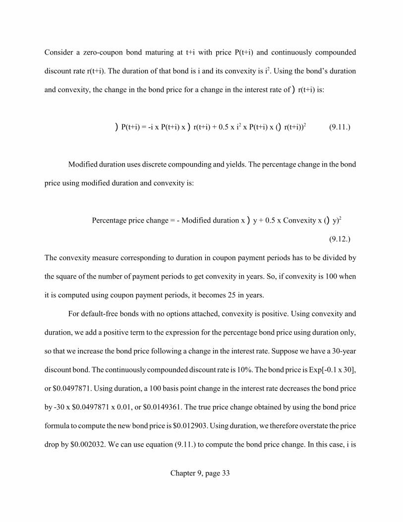
This adjustment term is called the bond’s convexity. The bond convexity is the change in the

bond’s duration for an infinitesimal change in yield. For a discount bond, the convexity is duration

squared. Convexity is expressed in the same units as the duration. Consequently, we have:

Bond price change using Fisher- Weil duration and convexity

Chapter 9, page 33

Consider a zero-coupon bond maturing at t+i with price P(t+i) and continuously compounded

discount rate r(t+i). The duration of that bond is i and its convexity is i2. Using the bond’s duration

and convexity, the change in the bond price for a change in the interest rate of )r(t+i) is:

)P(t+i) = -i x P(t+i) x )r(t+i) + 0.5 x i2 x P(t+i) x ()r(t+i))2 (9.11.)

Modified duration uses discrete compounding and yields. The percentage change in the bond

price using modified duration and convexity is:

Percentage price change = - Modified duration x )y + 0.5 x Convexity x ()y)2

(9.12.)

The convexity measure corresponding to duration in coupon payment periods has to be divided by

the square of the number of payment periods to get convexity in years. So, if convexity is 100 when

it is computed using coupon payment periods, it becomes 25 in years.

For default-free bonds with no options attached, convexity is positive. Using convexity and

duration, we add a positive term to the expression for the percentage bond price using duration only,

so that we increase the bond price following a change in the interest rate. Suppose we have a 30-year

discount bond. The continuously compounded discount rate is 10%. The bond price is Exp[-0.1 x 30],

or $0.0497871. Using duration, a 100 basis point change in the interest rate decreases the bond price

by -30 x $0.0497871 x 0.01, or $0.0149361. The true price change obtained by using the bond price

formula to compute the new bond price is $0.012903. Using duration, we therefore overstate the price

drop by $0.002032. We can use equation (9.11.) to compute the bond price change. In this case, i is

Chapter 9, page 34

equal to 30, and i squared is equal to 900. Consequently, the bond price change obtained using

equation (9.11.) is:

)P(t+i) = -i x P(t+i) x )r(t+i) + 0.5 x i2 x P(t+i) x ()r(t+i))2

= -30 x 0.0497871 x 0.01 + 0.5 x 900 x 0.0497871 x 0.0001

= 0.0126957

With the convexity adjustment, we now understate the price fall by $0.000207. Using convexity

reduces the absolute value of the mistake by a factor of 10 in this case.

Duration captures the first-order effect of interest rate changes on bond prices. The duration

hedge eliminates this first-order effect. Convexity captures the second-order effect of interest rate

changes. Setting the convexity of the hedged portfolio equal to zero eliminates this second-order

effect. To eliminate both the first-order and the second-order effects of interest rate changes, we

therefore want to take a hedge position that has the same duration and the same convexity as the

portfolio we are trying to hedge.

To understand how convexity can affect the success of a hedge, let’s go back to Investbank

Corp., but now we assume that it has a duration of 21 years and a convexity of 500 using the Fisher-

Weil duration instead of the modified duration. Suppose that we hedge with the 30-year discount

bond. This discount bond has a duration of 30 and a convexity of 900. The bank’s equity is worth

$20M. So, if we use only the 30-year bond, we have to go short $h of the discount bond, so that $h

x 30 x )r is equal to 21 x $20M x )r. The short position in the discount bond must therefore be for

0.7 x $20M, $14M. This gives Investbank Corp. a convexity of -130 (500 - 0.7 x 900). In this case,

Chapter 9, page 35

the hedged bank has negative convexity.

To see how interest rate changes affect the value of the bank, suppose the current interest rate

is 5% and the bank earns 8% on its equity over the next year if interest rates do not move. In this case,

the hedged bank’s value one year from now as a function of the interest rate then prevailing is given

in Figure 9.4. assuming that the bank has no duration and negative convexity of 130 in one year. In

this Figure, the value of the bank is a concave function of the interest rate. This value reaches a

maximum of $21.6657M at the current interest rate, which we take to be 5%. At that rate, the slope

of this function is zero if the bank is still hedged so that it has no duration. The current value of the

hedged bank’s equity, $20M, is the present value of its hedged payoff one year from now. Since the

bank value is highest if rates do not change, this means that if rates do not change, the bank value is

higher than expected and if rates change by much in either direction the bank value is lower than

expected. Hence, for the bank to earn a fair rate of return, it has to earn more than the risk-free rate

of 5% if interest rates do not change.

To improve the hedge, we can construct a hedge so that the hedged bank has neither duration

nor convexity. This requires us to use an additional hedging instrument so that we can make the

convexity of the hedged bank equal to zero. Let h be the short position in a discount bond with

maturity i and k be the short position in a discount bond with maturity j. We invest the proceeds of

the short positions in a money market instrument so that the value of the bank is unaffected by the

hedge. In this case, the hedge we need is:

Duration of unhedged bank = (h/Value of bank) x i + (k/Value of bank) x j

Convexity of unhedged bank = (h/Value of bank) x i2 + (k/Value of bank) x j2

Chapter 9, page 36

N

i 1

W P(t+i) x C(t+i)=

= ∑

Let’s use a discount bond of 30 years and one of 5 years. We then need to solve:

21 = (h/20) x 30 + (k/20) x 5

500 = (h/20) x 900 + (k/20) x 25

The solution is to have h equal to 10.5333 and k equal to 20.8002. In this case, the duration is

-(10.5333/20) x 30 + 21 - (20.8002/20) x 5, which is zero. The convexity is -(10.5333/20) x 900 +

500 - (20.8002/20) x 25, which is also zero.

We can estimate VaR using duration and convexity. Since any fixed income portfolio of

default-free bonds (with no options attached) can be decomposed into a portfolio of investments in

zero coupon bonds, we can model the random change in the value of the portfolio in a straightforward

way using the Fisher-Weil formulas for duration and convexity.

C(t+i) represents the portfolio cash flow in year t+i. For instance, if the portfolio holds one

coupon bond which makes a coupon payment at date i equal to c, C(t+i) is equal to c. In this case, the

value of the portfolio W is given by:

If we make discount bond prices depend on one interest rate only, r, then we have:

(9.13.)N N

2 2

i=1 i 1W= C(t+i) P(t+i) C(t+i) x (i x r 0.5 x i x ( r) )

=

∆ ∆ = ∆ − ∆∑ ∑

Chapter 9, page 37

Using this equation, we can then simulate the portfolio return by generating random changes in r and

use the fifth percentile portfolio value from the simulation as our VaR estimate.

Section 9.3.2.C. “Maturity bins” to protect against changes in the slope and shape of the term

structure

Duration protects a portfolio against changes in the level of the term structure. Level term

structure changes explain a large fraction of bond yield changes - at least 60% across countries. In the

U.S., level changes in the term structure explain more than 75% of the bond yield changes for U.S.

government bonds, and about 10% less for corporate bonds. In other words, we can expect to

eliminate a substantial fraction of the volatility of a bond portfolio through a duration hedge even

though not all interest rate changes correspond to level shifts in the term structure.

If all changes in yields for the assets and liabilities of a portfolio are brought about by parallel

shifts in the yield curve, the portfolio is hedged against small changes in interest rates if we make the

duration of the hedged portfolio zero. To hedge against larger changes in interest rates, we would also

choose a hedge portfolio that has a convexity of zero. With parallel shifts in the term structure, the

duration of the securities we use to hedge does not matter. This is a strength of duration, since it

allows us to use the most liquid bonds to hedge. Suppose a portfolio of $100M has a ten year

duration. We can hedge that portfolio by going short $1B of securities with one year duration. In this

case, the duration of the hedged portfolio is 10 x ($100M/$100M) - 1 x ($1B/$100M), or zero.

Alternatively, we could hedge by going short $50M of securities with a duration of 20. Whatever the

duration of the hedge, a 100 basis point increase in yields has no effect on the value of the portfolio

when its impact is evaluated using duration.

Chapter 9, page 38

If changes in the slope and shape of the term structure are a concern, it is no longer the case

that the duration of the security used to hedge does not matter. Suppose that we have a steepening of

the term structure associated with an increase in rates. The short end increases by 100 basis points

while the medium term and long term rates increase by 200 basis points. The yield of our portfolio

goes from 5% to 7%. Using duration, we lose 10 x $100M x 0.02, or $20M. If we hedged with a

security that had a one-year duration, we were short $1B of that security. Its yield increases only by

100 basis points. Therefore, we gain only $10M on our hedge, 1 x $1B x 0.01, and our hedged

portfolio loses $10M. Yet, had we hedged with the security that has a duration of 20 years, the yield

of that security would have increased by 200 basis points. Consequently, we would have gained 20

x $50M x 0.02, or $20M, so that we would have been perfectly hedged.

One way to construct a hedged portfolio whose value is insensitive to changes in the slope and

shape of the term structure is to start from the cash flows of the portfolio. We can then assign cash

flows to “maturity bins”. For instance, take all cash flows that are received or paid in a five year

period starting five years from now are put in one bin. Now, instead of hedging the whole portfolio

directly, we choose a hedging instrument that reflects discount bond rates for maturities

corresponding to the bin we are hedging and then set the duration of the bin equal to zero using that

instrument. This way the yield of the hedging instrument will move by the same amount as the yield

of the cash flows hedged.

To implement this approach, one has to have appropriate hedging instruments. In many

countries, such instruments are not available, while duration hedges can be implemented.

Section 9.4. Measuring and managing interest rate risk without duration

Chapter 9, page 39

Duration makes it possible to evaluate exactly the impact of an infinitesimal parallel shift in

the term structure. Duration requires a parallel shift and becomes less precise as the size of the shift

increases. Whether we use duration only or duration plus convexity, we have only an approximation

for interest rate changes that are not infinitesimal.

To estimate VaR, we have to use a distribution for interest rate changes. With distribution

fitted to actual data, there is some possibility of large changes in rates for which duration works

poorly. Further, changes for rates of different maturities are not perfectly correlated, so that we have

to be able to evaluate the impact of shifts in the term structure, which cannot be done with simple

duration approaches. Consequently, if we use duration to measure VaR, we ignore a potentially

important source of risk, namely risks associated with changes in the shape of the term structure. We

ignore changes in spreads among rates when we apply duration to bonds with credit risks, too. As

rates change, credit spreads can change also. For instance, there is empirical evidence that credit

spreads fall as interest rates increase. Bonds often have embedded options – for instance, the issuer

can call the bond, the holder can exchange the bond for another bond or stock, the holder can put the

bond, and so on. Whereas an institution with only high grade bonds with no embedded options may

not miss much if it uses duration, this is definitely not the case for institutions that hold bonds with

embedded options or bonds with more significant default risks.

The alternative to duration is direct consideration of the impact of interest rate changes on

prices. To see how an interest rate change affects the value of a fixed income position, we simply

compute the value of the position given the new interest rates. For instance, we can evaluate the

impact on the portfolio of a one basis point change in rates by recomputing the value of the portfolio

for that change. This approach is becoming increasingly common.

Chapter 9, page 40

A good example is the Chase Manhattan Bank. In 1999, Chase stopped reporting the gap

measures represented in Table 9.2. and started reporting the basis point value for its portfolio (BPV).

The BPV gives the change in the market value of a portfolio for a one basis point change in rates.

Before 1999, Chase used BPV for its trading portfolio only. Since 1999, it has used it more broadly

to include other assets and liabilities. Chase considers two different BPVs. First, it estimates the

impact of a one basis point change in interest rates. It reports that at the end of December 31, 1999,

the BPV for a one basis point change in rates was -$6.4M. Second, it computes the impact of a one

basis point change in spreads between liabilities and assets (basis risk). It reports that the BPV of a

one basis point change in spreads is -$10.7M.

Recomputing the portfolio value for different interest rates, we can compute the portfolio’s

VaR as well as construct minimum-volatility hedges. Computing power is the key. For instance, we

can estimate a joint distribution for the interest rates one is interested in, and use Monte Carlo

simulation to obtain draws of interest rates. For each draw of the interest rates, we compute the value

of the position. After a large number of draws, we end up with a simulated distribution of the value

of the position given the joint distribution of the interest rate changes. We can then use the fifth

percentile of that simulated distribution as our VaR and use the distribution to construct minimum-

volatility hedges. Alternatively, we could use historical changes in interest rates to obtain simulated

values of the position. This kind of approach was out of reach when Macaulay introduced his duration

measure. Repricing a fixed-income portfolio can now be implemented within minutes or hours.

A model in which all rates depend on only one random variable is called a one-factor model

of the term structure. In a one-factor model of the term structure, all rates depend on a single random

variable and are therefore perfectly correlated. The duration model is a one-factor model of the term

Chapter 9, page 41

structure; it allows only identical changes to all rates. To allow for rates to be imperfectly correlated,

we must allow for more sources of variation in rates. If we make the rates depend on two random

variables or sources of risk, we have a two-factor model of the term structure.

When we allow more sources of risk to affect interest rates, a wider range of changes in the

shape of the term structure becomes possible. Three alternate approaches to modeling interest rate risk

are possible. The first approach considers the distribution of the discount bond prices. The second

approach models spot interest rates as functions of factors. The third approach uses the distribution

of forward rates.

Section 9.4.1. Using zero coupon bond prices as risk factors

The simplest way to model the risk of a fixed income portfolio without using duration is to

simply use the joint distribution of the returns of the securities in the portfolio. If returns are normally

distributed, we know how to compute a VaR analytically. Knowing the joint distribution of the

returns of the securities, we could construct minimum-volatility hedges using the covariances and

variances of the returns of these securities.

This approach is a natural use of modern portfolio theory, but it runs into some serious

difficulties. The first difficulty is that, if we proceed this way, there are likely to be arbitrage

opportunities among our fixed-income securities. The portfolio might have many different bonds,

each with its own return. We know that to avoid arbitrage opportunities the law of one price must

hold: there can be only one price today for a dollar delivered for sure at a future date. This means that

if 20 different bonds pay a risk-free cash flow in 30 years exactly, all 20 bonds must discount that

risk-free cash flow at the same rate. This does not happen if we allow all bonds to have imperfectly

Chapter 9, page 42

correlated returns.

The second difficulty is that there are too many securities if we treat each security separately.

To eliminate arbitrage opportunities, we can start by generating discount bond prices and use

these bonds to price other bonds. This insures that all risk-free payoffs have the same prices across

bonds. This approach is popular in practice. In particular, it is the one used by Riskmetrics™. As

explained in Chapter 4, the risk model proposed by Riskmetrics™ is widely used. Riskmetrics™

makes available correlations and volatilities of the returns of selected discount bonds. Since any

default-free fixed-income security with no options attached is a portfolio of discount bonds, we can

figure the distribution of its return using Riskmetrics™. With this distribution of returns, a portfolio

of fixed-income securities is not treated differently from a portfolio of stocks. We know how to

compute the analytical VaR of portfolios of stocks, so we can compute an analytical VaR of portfolios

of discount bonds. In addition, since we know the distribution of the return of the portfolio, we can

also manage the risk of the portfolio by constructing a minimum-volatility hedge.

That the Riskmetrics™ distributions are only available for a subset of discount bonds creates

a difficulty. A country may have a five-year discount bond and a seven-year discount bond, but no

six-year discount bond. Yet, if we have a discount bond in that country, that discount will have a

coupon payment six years from now.

To use the Riskmetrics™ approach, we have to transform the coupon bond into a portfolio

of discount bonds. We therefore have to find a solution where we can know the distribution of the

return of the six–year discount bond. The approach recommended by Riskmetrics™ involves an

interpolation method that is described in Box 9.3. Riskmetrics™ and bond prices.

Chapter 9, page 43

Section 9.4.2. Reducing the number of sources of risk: Factor models

A different approach is to assume that a few risk factors explain changes in all bond prices.

The simplest such model assumes that returns on bonds depend on two factors, such as a short rate

and a longer maturity rate or a spread between long maturity and short maturity. The short rate is

intended to capture the level of the term structure and the spread or the long maturity rate capture the

steepness of the curve. When two risk factors are used to explain the term structure, we have a two-

factor model. A two-factor model explains returns on bonds better than the duration model, where

returns depend on only one factor model. A two-factor model explains about 10% to 20% more of

the returns of government bonds than the one factor model.

Factor analysis also can identify common factors that influence returns of discount bonds.

Suppose we have time-series information for a cross-section of variables, say bond returns for bonds

with different maturities. Factor analysis is a statistical technique that extracts from the data

explanatory variables, factors, that explain bond returns in a regression. Using this technique, analysts

extract factors from the data rather than pre-specify them. Litterman and Scheinkman (1991) find that

three factors explain at least 95% of the variance of the return of discount bonds. The three factors

extracted this way roughly correspond to a level effect, a steepness effect, and a curvature effect. The

level or duration effect explains at least 79.5% of the variance of the return of discount bonds. With

a time series of factor returns, we can estimate the exposure of each discount bond using a regression

of discount bond returns on factor returns.

A three-factor model like Litterman and Scheinkman’s can be used to hedge. They consider

a portfolio with a duration of zero shown in Table 9.3. That portfolio is bought on February 5, 1986,

and sold on March 5, 1986. Over that month, it loses $650,000. Using their three factors, they find

Chapter 9, page 44

that the portfolio loses $84,010 for a one-standard-deviation (monthly) shock to the level factor, gains

$6,500 for a one-standard deviation shock to the steepness factor, and loses $444,950 for a one-

standard deviation in the curvature factor. During the month, the level factor changes by -1.482

standard deviations, the steepness factor by -2.487 standard deviations, and the curvature factor by

1.453 standard deviations. To compute the total impact of these changes on the value of the portfolio,

we add up these effects:

Total change in portfolio value = -1.482 x (-$84,010) + -2.487 x $6,500 + 1.453 x (-$444,950) = -

$538,175

Since the portfolio has a duration of zero, we would predict no change in its value with a change in

rates. The problem is that duration ignores the great effect of changes in the curvature of the term

structure on the value of the portfolio. This three factor model captures this effect. To hedge the

portfolio with the three factor model, we would have to go short portfolios that mimic the factors.

For instance, we would take a position in a portfolio that mimics the curvature factor so that we gain

$444,950 for a one standard deviation move in the curvature factor. To hedge a portfolio that is

exposed to the three factors, we would therefore have to take positions in three factor mimicking

portfolios to set the exposure of the hedged portfolio to each one of the factors equal to zero.

Knowing the exposure of a position to the factors is useful for three reasons. First, if we know

the joint distribution of the factors, we can use this joint distribution to compute VaR. If the factor

returns are normally distributed, we can take a fixed-income position and compute an analytical VaR.

If the factors are normally distributed returns, and we have three factors, the return on a fixed-income

Chapter 9, page 45

position is equivalent to the return of a three-security portfolio, where each security corresponds to

a factor. We already know how to compute the VaR analytically in this case.

Second, knowing the exposure of a position to the factors allows us to construct a hedge

against this exposure. All we have to do is take a position in securities or futures contracts that have

factor loadings that cancel out the factor loadings of our fixed income position.

Finally, exposure to factors can be an active management tool. We may feel that exposure to

one of the factors is rewarding while exposure to the other factors is not. In this case, our

understanding of the factor exposures of our position and of individual securities allows us to make

sure that we are exposed to the right factor.

Section 9.4.3. Forward curve models

The duration, discount bond, and factor model approaches do not generally guarantee that

discount rates are distributed so that there cannot be arbitrage opportunities. This is unfortunate

because we do not expect to find pure arbitrage opportunities in the markets. If a term structure allows

for arbitrage opportunities, one ends up with prices that do not correspond to prices that one could

find in actual markets, and hence the value of the position one obtains is not right. A key requirement

for a term structure to exhibit no arbitrage opportunities is that if we have a discount bond that

matures at time t + i with price at t of P(t + i), and a discount bond that matures at time t + j with price

P(t + j), it must be the case that P(t + j) < P(t + i ) as maturity date t + i takes place before maturity

date t + j. The reasoning for this is straightforward. If P(t + i) is the less expensive bond, we can buy

that bond and sell the other bond short. We then make a profit today of P(t + j) - P(t + i) that we get

to keep. At date t + i, we keep the proceeds from the bond that matures in the risk-free asset. At date

Chapter 9, page 46

t + j, we use these proceeds to reverse the short sale.

The problem is that if we are not careful in generating draws of the term structure of interest

rates, we can end up with a discount bond that is more expensive than a discount bond that matures

sooner. For instance, if the one-day returns of two discount bond prices are normally distributed and

not perfectly correlated, there is always some probability that the bond with a short maturity ends up

being less expensive since one bond could increase in price and the other could fall. To avoid this

problem, we must therefore impose some structure on how term structures are generated.

A straightforward way to proceed to avoid arbitrage opportunities is to use the forward curve.

Let f(t + i) be the forward rate at t for delivery of a one-year discount bond t + i. Using continuous

compounding, f(t + i) is equal to the logarithm of P(t + i)/P(t + i + 1). The forward rates f(t + i), for

all future dates, define the forward curve. This curve differs from the term structure obtained using

yields of discount bonds or using coupon bonds. The traditional term structure curve is given by the

yields of coupon bonds. It is generally called the par curve since it gives the coupon yield of bonds

issued at par.

Figure 9.5. shows the curves for an upward-sloping term structure. For such a term structure,

the discount bond yield curve, usually called the zero (for zero coupon) curve, is above the par curve.

The yield of a par bond is a weighted average of the yields of the discount bonds that compose the

portfolio of discount bonds. The yield of the discount bond with the same maturity as the coupon

bond is the zero coupon bond in that portfolio that has the highest yield when the term structure is

upward sloping. The forward rate corresponding to the maturity of the discount bond is the six-month

rate implied by that discount bond and the one maturing six months later. With an upward-sloping

term structure, the forward rate is therefore higher than the yield of the discount bond because the

Chapter 9, page 47

yield of the discount bond increases as the maturity lengthens, which can be achieved only through

a higher implied yield for the next period of time. Figure 9.5. shows how the forward curve, the zero

curve, and the par curve relate to each other for an upward-sloping term structure.

From the forward curve, we can compute the value of any bond. To see this, note that we can

buy at t the equivalent of a coupon payment to be made at date t + i for forward delivery at date t +

i – 1.The value of the coupon payment to be made at t + i as of t + i – 1 is the coupon payment

discounted for one period. We can enter c forward contracts today where we agree to pay the forward

price at t + i – 1 for a discount bond whose value at t + i is $1. If F(t + i – 1) is the forward price today

for delivery of a discount bond at t + i – 1 that pays $1 at t + i, we pay F(t + i – 1)c at t + i – 1.

Remember that F(t + i – 1) = P(t + i)/P(t + i – 1), where P(t + i) is the price at t of a discount bond that

pays $1 at t + i. We can enter F(t + i – 1)c forward contracts to purchase discount bonds at t + i – 2

that pay each $1 at t + i – 1. By paying F(t + i – 2) x F(t + i – 1)c at t + i – 2, we therefore pay for a

portfolio of discount bonds and forward contracts that gives us c at t + i. We can then go backward

one period, so that we enter F(t + i – 2) x F(t + i – 1)c forward contracts with forward price F(t + i –

3) at t to purchase discount bonds at t + i – 3 that pays $1 at t + i – 2. Therefore, by paying F(t + i –

3) x F(t + i – 2) x F(t + i – 1)c at t + i – 3, we acquire a portfolio of discount bonds and forward

contracts that pays c at t + i. We can then work backward from t + i – 3 up to today using the forward

contracts, so that we end up with the price of the coupon today. Suppose that t + i = t + 4. Then, F(t

+ i – 3) x F(t + i – 2) x F(t + i – 1)c = F(t + 1) x F(t + 2) x F(t + 3)c. We can buy F(t + 1) x F(t + 2)

x F(t + 3)c discount bonds at t for P(t + 1) per bond that pays $1 at t + 1. Consequently, the current

value of the coupon paid at t + 4 is P(t + 1) x F(t + 1) x F(t + 2) x F(t + 3)c. Note that P(t + 1) is also

the forward price at t for immediate delivery with price F(t), so that we can write the present value

Chapter 9, page 48

Value of coupon today=F(t) x F(t+1) x F(t+2)...F(t+i 2) x F(t+i 1) x c

P(t+1) P(t+i 1) P(t+i)= ... x cP(t) P(t+i 2) P(t+i 1)

=P(t+i) x c

− −−− −

-r(t) -f(t + 1) -f(t+i 3) -f(t+i 2) -f(t+i 1)

-[r(t) + f(t + 1)... + f(t+i 3) + f(t+i 2) + f(t+i

P(t+1) P(t+i 1) P(t+i)Present value ofcoupon payment at t+i = ... x cP(t) P(t+i 2) P(t+i 1)

=e x e ...e x e x e x c=e

− − −

− −

−− −

1)] x c−

of the coupon as F(t) x F(t + 1) x F(t + 2) x F(t + 3)c. More generally, using our reasoning, we have:

(9.16.)

P(t) is the price of a discount bond that matures at t and is therefore 1. Using this expression, we can

use the forward curve to compute the value of future cash flows. We can therefore also compute the

risk of the value of the coupon today by using the distribution of the forward prices or the forward

rates since:

(9.17)

Note that the discount rate in the last line is the sum of the one-period forward rates plus the current

spot rate. If we use the forward rates, we start from the current forward rates. We can then estimate

the joint distribution of the forward rates. Having this joint distribution, we can simulate forward

curves and value the portfolio for each simulated forward curve.

There is an important difference between the forward curve approach and the approaches that

use zero-coupon bond prices or rates for various maturities. With continuous compounding, the

discount rate that applies to a bond maturing at t+i is the sum of the forward rates as we just saw.

Hence, any change in a forward rate affects the discounting rate for a discount bond with a maturity

Chapter 9, page 49

that is later than the period for which the forward rate is computed. A shock to the forward rate for

maturity t+i has a one-for-one effect on the discount rate of all discount bonds that mature later. If we

instead simulate discount bonds using the joint distribution of discount bond returns, a price

realization of the price of discount bond for one maturity could be high without affecting the price

of the discount bonds maturing later on because of the risk of the bond uncorrelated with the risk of

other bond prices. The same could be the case if one uses discount rates instead of discount bond

prices. The forward rate approach therefore insures that the no-arbitrage condition holds for the term

structure.

We can obtain simulated forward curves in essentially two ways. One way is to use the

historical changes in the forward curve. To do that, we compute either absolute changes or

proportional changes of the forward curve over past periods. If we want to estimate a one-month VaR,

we use monthly changes. Whether we use absolute or proportional changes depends on whether we

believe that the distribution of absolute or proportional changes is more stable. There are good

arguments to use proportional changes since, when interest are low, we would think that a one

hundred basis point change in rates is not as likely as when rates are low.

Computing changes using past history allows us to construct a database of changes. We can

then apply these changes to the current term structure to obtain simulated term structures for which

we compute portfolio values. The fifth percentile of these portfolio values gives us the VaR.

Alternatively, we can estimate the joint statistical distribution of changes in the forward curve

using past data. For instance, we could assume that proportional changes are jointly normally

distributed and then estimate the parameters for this joint distribution. Then, we could use that

distribution for a Monte Carlo analysis. With this analysis, we would draw forward curves and price

Chapter 9, page 50

the portfolio for these forward curves to get a VaR. We could also assume that forward rate changes

follow a factor model, so that the whole forward curve changes depend on relatively few sources of

risk.

Section 9.5. Summary

A firm’s mix of floating and fixed rate debt is a risk management tool. If the firm at a

particular time sees it has the wrong mix, it can change the mix by refinancing or by using derivatives.

We can transform floating rate debt into fixed rate debt using the Eurodollar futures contract. A

financial institution’s interest rate exposure can be evaluated in terms of the effect of interest rate

changes on income or on value. We show how one can compute CaR for a financial institution. To

compute VaR for a financial institution, we have to understand how changes in interest rates affect

the value of the securities held by that institution. Traditionally, duration has been the most popular

tool for such an assessment. There are various ways to implement the duration. Modified duration is

computed using bond yields. With the Fisher-Weil duration, we transform a coupon bond into a

portfolio of discount bonds and use the interest rates of these discount bonds to compute duration.

Finally, we can add convexity to duration to take into account the nonlinear relation between bond

prices and interest rates. Whatever duration we use, we can compute a duration-based VaR. In the last

section of the chapter, we consider ways of computing VaR and evaluating interest rate risk that do

not rely on duration but rather evaluate the impact of interest rate changes on the value of fixed-

income securities directly. One approach, proposed by Riskmetrics™, treats zero-coupon bond prices

as risk factors. Another approach treats interest rates as risk factors. The last approach treats forward

rates as risk factors.

Chapter 9, page 51

Key concepts

Forward rate agreements, notional amount, asset sensitive, LIBOR, asset sensitive, liability sensitive,

dollar maturity gap, stress test, modified duration, Fischer-Weil duration, bond convexity, interest rate

delta exposure, factor models, forward curve.

Chapter 9, page 52

Review questions

1. What is floating-rate debt?

2. What is LIBOR?

3. What is the reset date?

4. What is a FRA?

5. How do you interpret a Eurodollar Futures Index of 92?

6. What does it mean to say that a bank is liability sensitive?

7. How do you define the dollar maturity gap for the period from 1 to 5 years?

8. What is a stress test?

9. How do you estimate the impact of a change in yield on a bond price using modified duration?

10. How does Fisher-Weil duration differ from modified duration?

11. How does the additional use of convexity affect your estimate of the impact of a change in yield

on a bond price obtained using modified duration only?

12. What is BPV?

13. What is a factor model for interest rates or discount bond returns?

14. What is a forward curve model?

15. Which approach in modeling the risk of a fixed-income portfolio guarantees that there are no

arbitrage opportunities between the discount bond prices generated through a draw of a Monte Carlo

simulation?

Chapter 9, page 53

Questions and exercises

1. A firm has fixed income of $10m per year and debt with face value of $100m and twenty-year

maturity. The debt has a coupon reset every six months. The rate which determines the coupon is the

6-month LIBOR. The total coupon payment is half the 6-month LIBOR on the reset date in decimal

form times the face value. Today is the reset date. The next coupon has just been set and is to be paid

in six months. The 6-month LIBOR at the reset date is 5.5% annually. The volatility of 6-month

LIBOR is assumed to be 100 basis points annually and the term structure is flat. What is the one-year

CaR for this firm assuming that the only risk is due to the coupon payments on the debt?

2. What is the value of the debt at the reset date if the debt has no credit risk? What is the duration

of the debt at the reset date if the debt has no credit risk?

3. A position has modified duration of 25 years and is worth $100m. The term structure is flat. By

how much does the value of the position change if interest rates change by 25 basis points?

4. Suppose that you are told that the position has convexity of 200 years. How does your answer to

question 3 change?

5. Consider a coupon bond of $100m that pays coupon of $4m and has no credit risk. The coupon

payments are in 3, 9, and 15 months. The principal is paid in 15 months as well. The zero-coupon

bond prices are P(t+0.25) = 0.97531, P(t+0.75) = 0.92427, and P(t+1.25) = 0.82484. What is the

Chapter 9, page 54

current bond price? What is the forward price today for a six-month zero-coupon bond delivered in

9 months? What is the forward rate associated with that forward price?

6. Using the Fisher-Weil duration, compute the impact of a parallel shift in the yield curve of 50-basis

points? How does your answer compare to the change in the bond price you obtain by computing the

new bond price directly and subtracting it from the bond price before the parallel shift?

7. Compute the yield of the bond and then compute the modified duration using the data in question

5. What is the impact of a 50 basis points change in the yield using the modified duration? How does

it compare to your answer in question 6? How does your answer compare to the change computed

directly from the new and the old bond prices?

8. How does your answer to question 7 change if you also use convexity?

9. Assume that the volatility of the zero-coupon bond prices expressed per year in question 5 is 1%

for the 3-month bond, 3% for the 9-month bond, and 5% for the 15-month bond. The correlation

coefficients of the bonds are 0.9 between all bonds. Ignoring expected changes in value of the bonds,

what is the volatility of the bond price? Assuming that the returns of the zero-coupon bond prices are

normally distributed, what is the one-day VaR of the bond?

10. Show how the par curve, the zero curve, and the forward curve relate to each other if the term

structure is downward sloping.

Chapter 9, page 55

Technical Box 9.1. The tailing factor with the Euro-dollar futures contract

We are at date t and want to hedge an interest rate payment to be made at date t+0.5 based on an

interest rate determined at date t+0.25, the reset date. We therefore want to use a Euro-dollar futures

contract that matures at date t+0.25. Let’s define F to be the implied futures yield at date t for the

contract that matures at t. Settlement variation on the contract at t+0.25 is 0.25 x (RL(t+0.25) - F)

times the size of the short position. At t+0.25, we get to invest the settlement variation for three

months at the rate of RL(t+0.25). This means that at t+0.5 we have (1+0.25 x RL(t+0.25)) x (0.25 x

(RL(t+0.25)-F)) times the short position. We therefore want to choose a short position h such that at

t+0.5 we have no interest rate risk. The net cash flow at t+0.5 is equal to minus the interest payment

plus the proceeds of the short position:

- 0.25 x RL(t+0.25) x 100M +

h x (1+0.25 x RL(t+0.25)) x 0.25 x (RL(t+0.25)-F)

If we choose h so that at t+0.25 it is equal to 100M/(1+0.25 x RL(t+0.25)), we end up with:

- 0.25 x RL(t+0.25) x 100M +

(100M/(1+0.25 x RL(t+0.25)) x (1+0.25 x RL(t+0.25)) x (0.25 x (RL(t+0.25)-F))

= -0.25 x F x 100M

Consequently, if h is such that at date t+0.25 its value is 100M/(1+0.25 x RL(t+0.25)), we eliminate

Chapter 9, page 56

the interest rate risk and our net cash flow at date t+0.5 is equal to an interest payment based on the

futures yield known when we enter the futures contract.

To have a futures position of 100M/(1+0.25 x RL(t+0.25)) at date t+0.25, note that 1/(1+0.25

x RL(t+0.25)) at date t+0.25 is the present value of one dollar paid at t+0.5 discounted at the LIBOR

rate. This must be equivalent to the value at t of a discount bond maturing at t+0.5 which has a risk

equivalent to LIBOR time-deposits. Therefore, if we use as the tailing factor such a discount bond

that matures at t+0.5, we will have the appropriate futures position at t+0.25. At date t, we therefore

take a short position equal to 100m times the price of such a discount bond. At date t, the price of

such a bond is the price of a dollar to be paid at t+0.5 discounted at six-month LIBOR.

Chapter 9, page 57

Technical Box 9.2. Orange County and VaR

To see that a VaR computation using duration can provide extremely useful information, let’s look

at the case of Orange County. In December 1994, Orange County announced that it had lost $1.6

billion in an investment pool. The investment pool collected funds from municipalities and agencies

and invested them on their behalf. The pool kept monies to be used to finance the public activities of

the County. The amount in the pool had been $7.5 billion and was managed by the County Treasurer,

Bob Citron. As of April 30, 1994, the portfolio had an investment in securities of $19.860b with

reverse repo borrowings of $12.529b. The securities were mostly agency fixed-rate and floating rate

notes with an average maturity of about 4 years. The fund was therefore heavily levered. The

investment strategy was to borrow short-term using the repo market discussed in Chapter 2 to invest

in securities with longer duration to take advantage of the slope of the term structure. The problem

with such a strategy is that as interest rates increase, the value of the assets falls while the liabilities

do not. Valuing the securities held on April 30 at cost, we have $19,879b worth of assets. The

duration of the pool was estimated at 7.4 in a subsequent analysis. The yield of the five-year note went

from 5.22% in December 1993 to 7.83% in December 1994. Let’s assume that 7.4 is the appropriate

duration for December 1993 and that the portfolio given in the table is the one that applies at that

time. Assuming further that this duration measure is modified duration and that the yield of the 5-year

note is the appropriate yield given the duration of the pool, we have the loss to the pool for a 261 basis

points change in rates:

7.5B x 7.4 x 0.0261 = $1.406B

Chapter 9, page 58

This is quite close to the actual loss reported of $1.6B. Let’s assume that percentage changes in yields

are normally distributed. Using monthly data from January 1984 to December 1993, the volatility for

the percentage change in the yield of the 5-year note is 4.8% per month. Applying the square-root

rule, this gives us a yearly proportional volatility of 16.63%. The 5-year note had a yield of 5.22% in

December 1993, so that 16.63% of 5.22% is 0.868%. There was therefore a 5% chance that the 5-year

yield would increase by more than 1.65 x 0.868% over the coming year, or more than 1.432%. The

loss corresponding to an increase of 1.432% is given by the duration formula:

One-year VaR = 1.65 x 7.5B x 7.4 x 0.01432 = $1.31135B

In other words, as of December 1993, the one-year VaR of the Orange County pool was $1.31135B.

There was therefore a five percent chance Orange County would lose at least $1.31135B given its

investment strategy based on the assumptions of this calculation. Obviously, many refinements could

be made to this calculation. However, it shows that the duration VaR tool can be sufficient to

understand risk well enough to avoid big mistakes. It is hard to believe that the officials of Orange

County would have used the investment strategy they chose had they known the VaR estimate we just

constructed.

Sources: The Orange County debacle is described in Philippe Jorion, Big bets gone bad: Derivatives

and bankruptcy in Orange County, Academic Press, 1995. Professor Jorion also maintains a Web Site

that includes a case on Orange County involving various VaR computations for December 1994 and

useful other materials: http://www.gsm.uci.edu/~jorion/oc/case.html.

Chapter 9, page 59

Technical Box 9.3. Riskmetrics™ and bond prices

The Riskmetrics™ approach to evaluating interest rate risk involves two steps. The first step

consists in mapping cash flows from fixed income securities to the cash flows available from

Riskmetrics™. These cash flows are called vertices in the language of Riskmetrics™. In our

language, this operation amounts to matching the cash flows of default-free fixed income securities

to the cash flows of zero-coupon bonds. Through this operation, the portfolio of fixed income

securities is transformed into an equivalent portfolio of zero-coupon bonds. Its return then becomes

the return of a portfolio of zero-coupon bonds. Riskmetrics™ makes available the volatilities and the

correlations of the returns of these zero-coupon bonds. We can therefore compute an analytical VaR

using this information and using as portfolio weights the investments in the zero-coupon bonds of the

transformed portfolio.

The complication with the Riskmetrics™ approach is that there are at most 14 vertices

available - 1m, 3m, 6m, 12m, 2yr, 3yr, 4yr, 5yr, 7yr, 9yr, 10yr, 15yr, 20yr, 30yr. Obviously, a portfolio

will have cash flows with maturities that do not correspond to the vertices. For instance, a portfolio

might have a cash flow that matures in 6 years. The solution is then to attribute that cash flow to the

two adjoining vertices, 5 year and 7 year, in a way that does not affect the risk of the portfolio

compared to what it would be if we had the 6 year vertex. This means that (a) the total value of the

cash flow must not be affected by the split, (b) the market risk must be preserved, and (c) the sign

is preserved.

The implementation of the approach works by first interpolating the yields linearly. In our

example, the 6-year yield is half the 5-year and half the 7-year. With the interpolated 6-year yield, we

can compute the present value of the 6-year cash flow. The volatility of the 6-year return is computed

Chapter 9, page 60

by taking a linear interpolation of the 5-year and 7-year volatilities. We then solve for weights on the

5-year and the 7-year zeroes so that the variance of this portfolio of two zeroes has the same variance

as the 6-year return and the same value. These weights are then used to split the 6-year cash flow into

a 5-year and a 7-year cash flow. The Table Box 9.1. reproduces an example from the Riskmetrics™

manual.

Table Box 9.1. Riskmetrics™ mapping of cash flows

Problem:On July 31, 1996, we expect a cash flow occurring in 6 years of USD 100.

Data fromRiskmetrics™:

r(t+5) r(t+7)1.65std(r(t+5))

1.65std(r(t+7))

D(r(t+5),r(t+7))

5-year yield7-year yieldRiskmetrics™ volatility on the 5-year bond price returnRiskmetrics™ volatility on the 7-year bond price returnCorrelation between the 5-year andthe 7-year bond return

6.605%6.745%0.5770%

0.8095%

0.9975

Interpolation ofyields

0.5 x 6.605% + 0.5 x 6.745% 6.675%

Standarddeviation ofr(t+6)

0.5 x (0.5770%/1.65)+ 0.5 x (0.8095%/1.65)

0.4202%

Variance ofr(t+6)r(t+5)r(t+7)

1.765*10-3%1.223*10-3%2.406*10-3%

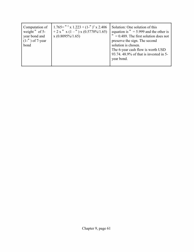
Chapter 9, page 61

Computation ofweight " of 5-year bond and(1-") of 7-yearbond

1.765= "2 x 1.223 + (1-")2 x 2.406+ 2 x " x (1 – ") x (0.5770%/1.65) x (0.8095%/1.65)

Solution: One solution of thisequation is " = 5.999 and the other is" = 0.489. The first solution does notpreserve the sign. The secondsolution is chosen. The 6-year cash flow is worth USD93.74. 48.9% of that is invested in 5-year bond.

Chapter 9, page 62

Table 9.1. Eurodollar futures prices.

EurodollarDaily Prices As of :- Wednesday, 10 May

Date Open High Low Last Chge Prev. Prev.Volume Open_Int

5/10/00 M a y00

932700

932850 932650 932775 125 1520 35446

5/10/00 J u n00

931400

931650 931350 931500 50 50676 503450

5/10/00 Jul 00 930200

930300 930200 930250 100 451 7331

5/10/00 A u g00

929350

929400 929100 929150 300 41 2540

5/10/00 S e p00

928050

928500 928000 928100 150 82742 563283

5/10/00 Oct 00 926000

926400 926000 926400 500 0 35

5/10/00 D e c00

925300

925950 925050 925450 350 74909 458937

5/10/00 M a r01

924500

925200 924250 924750 450 60037 359860

5/10/00 J u n01

923650

924400 923550 924000 500 34372 247951

5/10/00 S e p01

923400

924100 923300 923750 500 21612 186444

5/10/00 D e c01

922950

923700 922900 923300 450 10536 137124

5/10/00 M a r02

923450

924000 923300 923800 500 10597 126764

5/10/00 J u n02

923550

924000 923500 923900 550 5784 88815

5/10/00 S e p02

923600

924000 923450 923900 550 4897 87919

5/10/00 D e c02

923150

923550 922950 923450 550 4286 72646

5/10/00 M a r03

923650

924050 923350 923950 550 4950 72575

5/10/00 J u n03

923350

923750 922950 923700 600 2148 49702

5/10/00 S e p03

923150

923550 922750 923500 600 4117 49648

5/10/00 D e c03

922550

922950 922100 922900 600 1837 37798

5/10/00 M a r04

922950

923350 922500 923300 600 2019 32982

5/10/00 J u n04

922550

922950 922100 922900 600 1912 29965

5/10/00 S e p04

922250

922650 921800 922600 600 2320 25471

Chapter 9, page 63

5/10/00 D e c04

921550

921950 921100 921900 600 2557 26416

5/10/00 M a r05

921900

922300 921450 922250 600 2135 18824

5/10/00 J u n05

921300

921900 921100 921900 600 288 11228

5/10/00 S e p05

920950

921550 920750 921550 600 276 9930

5/10/00 D e c05

920250

920800 920050 920800 550 201 7055

5/10/00 M a r06

920500

921050 920300 921050 550 201 7478

5/10/00 J u n06

920350

920700 919950 920700 550 170 6494

5/10/00 S e p06

920000

920350 919600 920350 550 145 6108

5/10/00 D e c06

919300

919650 918900 919600 500 145 6085

5/10/00 M a r07

919650

919900 919150 919850 500 145 4740

5/10/00 J u n07

919000

919550 918800 919500 500 97 3798

5/10/00 S e p07

918700

919250 918500 919150 450 72 3647

5/10/00 D e c07

918000

918550 917800 918400 400 72 5130

5/10/00 M a r08

918250

918800 918050 918650 400 97 4289

5/10/00 J u n08

917900

918450 917700 918300 400 243 4593

5/10/00 S e p08

917550

918100 917350 917950 400 217 4152

5/10/00 D e c08

916850

917400 916650 917200 350 241 3180

5/10/00 M a r09

917550

917650 916900 917450 350 240 2647

5/10/00 J u n09

916550

917300 916550 917100 350 55 2554

5/10/00 S e p09

916200

916950 916200 916750 350 55 2438

5/10/00 D e c09

915500

916250 915500 916050 350 55 1724

5/10/00 M a r10

916400

916500 915750 916300 350 55 692

Composite V o l ume

Open_Int

5/9/00 389526

3319890

eRepresents net repricing effect of derivative positions, which include interest rate swaps,futures, forward rate agreements and options, that are used as part of Chase’s overall asset-liability management.

Chapter 9, page 64

Table 9.2. Interest Rate Sensitivity Table for Chase ManhattanThe balance sheet row represents the difference in value between the assets that reprice within aperiod and the liabilities that reprice during the same period.

At December 31, 1998 ( inmillions)

1-3 Months 4-6 Months 7-12 Months 1-5 years Over 5years

Balance Sheet $(37,879) $480 $6,800 $43,395 $(12,796)

Derivative Instruments AffectingInterest Rate Sensitivitye

(4,922) 803 (2,788) 2,542 4,365

Interest Rate Sensitivity Gap (42, 801) 1,283 4,012 45,937 (8,431)

Cumulative Interest RateSensitivity Gap

$(42,801) $(41,518) $(37,506) $8,431 $--

% of Total Assets (12)% (11)% (10)% 2% –%

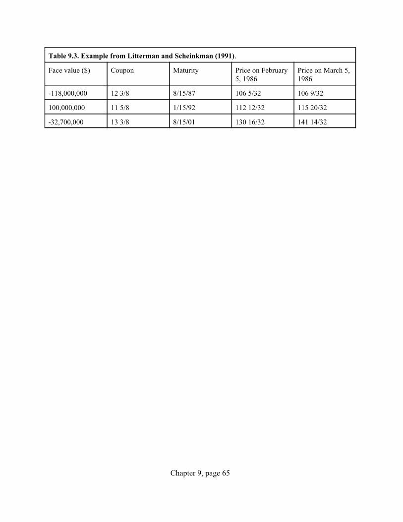
Chapter 9, page 65

Table 9.3. Example from Litterman and Scheinkman (1991).

Face value ($) Coupon Maturity Price on February5, 1986

Price on March 5,1986

-118,000,000 12 3/8 8/15/87 106 5/32 106 9/32

100,000,000 11 5/8 1/15/92 112 12/32 115 20/32

-32,700,000 13 3/8 8/15/01 130 16/32 141 14/32

Chapter 9, page 66

0%

2%4%

6%

8%

10%12%

14%

16%

0 5 10 15 20 25 30Time-to-maturity (Years)

0%2%4%6%8%

10%12%14%16%

0 5 10 15 20 25 30Time-to-maturity (Years)

Figure 9.1. Example of a Federal Reserve monetary policy tightening.

A. Term structure in March 1979. B. Term structure in March 1980.

Chapter 9, page 67

Figure 9.2. Bond price as a function of yield. This figure shows the price of a bond paying coupon annually of $5 for 30 years with principal value of $100.

Chapter 9, page 68

Figure 9.3. The mistake made using delta exposure or duration for large yield changes.

Chapter 9, page 69

Figure 9.4. Value of hedged bank. This figure shows the value of the hedged bank when the hedged bank has a duration of 21 years and aconvexity of 500. The bank is hedged with a discount bond with maturity of 30 years. This discount bond hasa duration of 30 years and a convexity of 900. The hedged bank has no duration at the current rate but hasnegative convexity. (Note that the present value of the hedged bank cannot be $20M. The present value of thehedged bank is the present value of the payoff represented in this figure. Hence, the bank will be worth morethan expected if rates do not change and will be worth less if they change by much.)

Bank value

Decimal interest rate

Chapter 9, page 70

YieldYield

Time to maturityTime to maturity00

Forward rateForward rateZeroZero--coupon yieldcoupon yieldCouponCoupon--bearingbearingbond yieldbond yield

Figure 9.5.Term Structures.

Chapter 9, page 71

Literature note

There are a large number of useful books on fixed income markets. Fabozzi (1996) provides the ideal

background. More advanced books include Ho (1990) and Van Deventer and Imai (1997). Van

Deventer and Imai (1997) have a more formal treatment of some of the arguments presented here.

Their book also covers some of the topics discussed in Chapter 14. That book also has a lot of

material on how to construct smooth term structures. Duffie (1994) reviews the issues involved in

interest rate risk management and presents the forward rate approach that we discuss in this chapter.

The paper by Litterman and Schenkman (1991) addresses the key issues involved in factor models.

Ilmanen (1992) presents an up-to-date empirical assessment of duration that supports our discussion.

Bierwag, Kaufman, and Toevs (1983) provide a nice collection of papers evaluating duration in a

scientific way. Ingersoll, Skelton, and Weil (1978) provide the Fisher-Weil duration measure

discussed in the text and relate it to the work of Macaulay. The Riskmetrics™ manual provides

complete information on how Riskmetrics™ deals with interest rate risks. Duffee (1998) shows that

credits spreads are negatively related to interest rates.