CHAPTER 8 ST 544, D. Zhang 8 Models for Matched Pairs

CHAPTER 8 ST 544, D. Zhang

8 Models for Matched Pairs

I Comparing Two Probabilities Using Dependent Proportions

• Example: Opinion relating to environment (Table 8.1 from 2000 GSS)

Cut living standard (Y2)

Yes (1) No (0)

Pay higher taxes (Y1) Yes (1) 227 132 359

No (0) 107 678 785

334 810

n = 1144 Americans. Here each subject is matched with

himself/herself to get Y1 and Y2.

We are interested in comparing π1 = P [Y1 = 1] and π2 = P [Y2 = 1].

We are not very interested in testing Y1 ⊥ Y2.

Slide 366


• If we convert table to

Yes No

Pay higher taxes 359 785 1144

Cut living standard 334 810 1144

P [Y1 = 1]: π1 = 359/1144 = 0.314

P [Y2 = 1]: π2 = 334/1144 = 0.292

Difference π1 − π2 = 0.022

var(π1 − π2)?

No way to get var(π1 − π2) if data is summarized using this table.

Need to go back to the original table!

Slide 367


I.1 Proportion difference using a matched sample

• Data and probability structure

Y2

1 0

Y1 1 n11 n12

0 n21 n22

Y2

1 0

Y1 1 π11 π12

0 π21 π22

π1 = P [Y1 = 1] = π11 + π12,

π2 = P [Y2 = 1] = π11 + π21.

Difference δ = π1 − π2 = π12 − π21.

Given data, the MLE of πij ’s: πij = nij/n

⇒δ = π12 − π21 =

n12 − n21

n.

Slide 368


var(δ) =π12(1− π12)

n+π21(1− π21)

n+

2π12π21

n

var(δ) =π12(1− π12)

n+π21(1− π21)

n+

2π12π21

n

=n12(n− n12) + n21(n− n21) + 2n12n21

n3

=(n12 + n21)− (n12 − n21)2/n

n2

• For our example,

δ = 0.022

var(δ) =(132 + 107)− (132− 107))2/1144

11442=

238.45

11442

SE(δ) =

√238.45

1144= 0.0135

Wald Test : χ2 = (0.022/0.0135)2 = 2.66

95% Wald CI of δ : 0.022± 1.96× 0.0135 = [−0.005, 0.048]

Slide 369


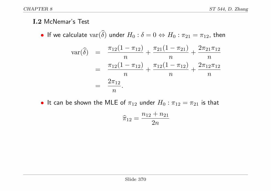
I.2 McNemar’s Test

• If we calculate var(δ) under H0 : δ = 0 ⇔ H0 : π21 = π12, then

var(δ) =π12(1− π12)

n+π21(1− π21)

n+

2π21π12

n

=π12(1− π12)

n+π12(1− π12)

n+

2π12π12

n

=2π12

n.

• It can be shown the MLE of π12 under H0 : π12 = π21 is that

π12 =n12 + n21

2n

Slide 370


⇒

var(δ)H0=

2

n× n12 + n21

2n=n12 + n21

n2

χ2 =δ2

var(δ)H0

=(n12 − n21)2/n2

(n12 + n21)/n2

=(n12 − n21)2

n12 + n21

H0∼ χ21

This is the McNemar’s test.

• For our example, McNemar’s χ2 = (132− 107)2/(132 + 107) = 2.615.

Do not reject H0 : π12 = π21 at level 0.05.

Slide 371


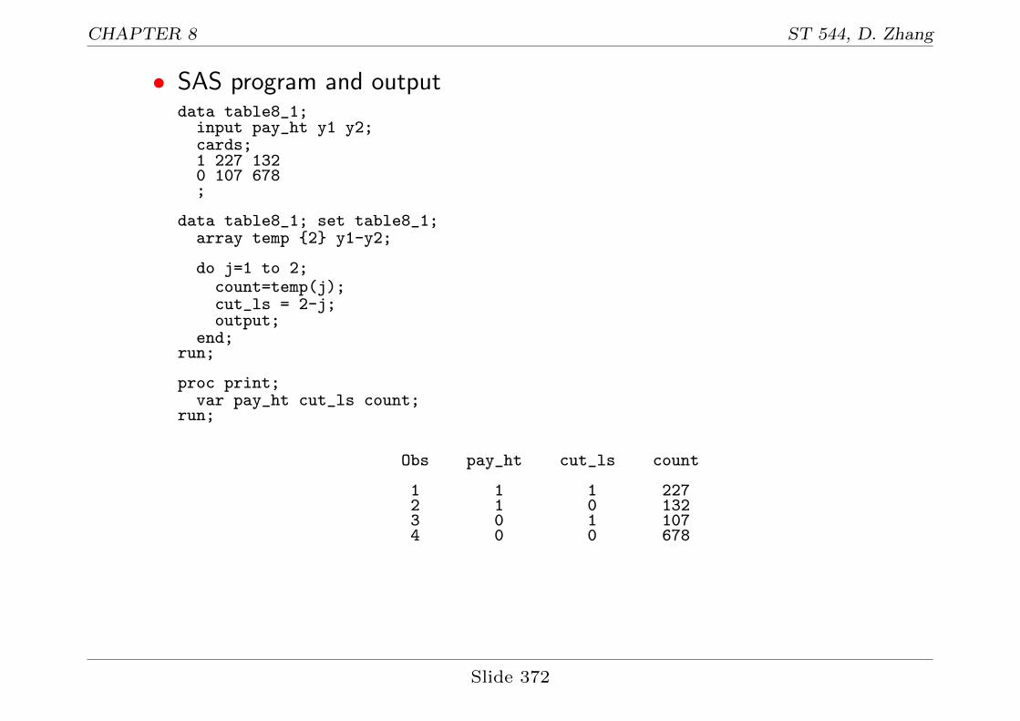
• SAS program and outputdata table8_1;

input pay_ht y1 y2;cards;1 227 1320 107 678;

data table8_1; set table8_1;array temp {2} y1-y2;

do j=1 to 2;count=temp(j);cut_ls = 2-j;output;

end;run;

proc print;var pay_ht cut_ls count;

run;

Obs pay_ht cut_ls count

1 1 1 2272 1 0 1323 0 1 1074 0 0 678

Slide 372


proc freq order=data;weight count;tables pay_ht*cut_ls / ;test agree;

run;

**************************************************************

Statistics for Table of pay_ht by cut_ls

McNemar’s Test-----------------------Statistic (S) 2.6151DF 1Pr > S 0.1059

Slide 373


• Note: The McNemar’s test can be derived from the Pearson χ2 test.

Under H0 : π12 = π21, the MLE’s of πij are

π11 =n11

n, π12 = π21 =

n12 + n21

2n, π22 =

n22

n.

The Pearson χ2 test for H0 : π12 = π21 is

χ2 =(n11 − nπ11)2

nπ11+

(n12 − nπ12)2

nπ12+

(n21 − nπ21)2

nπ21+

(n22 − nπ22)2

nπ22

= 0 +(n12 − n21)2

2(n12 + n21)+

(n12 − n21)2

2(n12 + n21)+ 0

=(n12 − n21)2

n12 + n21,

with df = 3− 2 = 1. This is the same as the McNemar’s test.

Slide 374


II GLM/Logistic Model for Matched Data

II.1 Marginal probabilities, population-level odds-ratio

• Risk difference from the converted table:

Y

X Yes (1) No (0)

Pay higher taxes (1) 359 785 1144

Cut living standard (0) 334 810 1144

Let π(x) = P [Y = 1|X = x]. If we fit a GLM link to π(x) with the

identity

π(x) = α+ βx,

then β = δ, the risk difference.

As we indicated before, var(δ) cannot be derived from this table and

we need to go back to the original table

Slide 375


• The formula var(δ) can be obtained by fitting the above GLM to the

data by recovering the original data at subject level and recognizing

the dependence of two observations from the same subjects.

• Each subject has two binary data points yi1, yi2

Y

X Yes (1) No (0)

Pay higher taxes (1) yi1 1− yi1 1

Cut living standard (0) yi2 1− yi2 1

• There are only 4 types of such tables:

Y

1 0

X 1 1 0

0 1 0

Type I: 227

1 0

1 0

0 1

II: 132

1 0

0 1

1 0

III: 107

1 0

0 1

0 1

IV: 678

Slide 376


• SAS program and part of output:title "Recover the individual data";data newdata; set table8_1;

retain id;if _n_=1 then id=0;

do i=1 to count;id = id+1;do question=1 to 2;

x = 2-question;if question=1 then

y=pay_ht;else

y=cut_ls;output;

end;end;

run;

proc genmod data=newdata descending;class id;model y = x / dist=bin link=identity;repeated subject=id / type=un;

run;

***********************************************************************

Analysis Of GEE Parameter EstimatesEmpirical Standard Error Estimates

Standard 95% ConfidenceParameter Estimate Error Limits Z Pr > |Z|

Intercept 0.2920 0.0134 0.2656 0.3183 21.72 <.0001x 0.0219 0.0135 -0.0046 0.0483 1.62 0.1055

Slide 377


• The approach we used to account for the dependence of observations

from the same subjects is called GEE (for generalized estimating

equation). We will talk about GEE in more detail in Chapter 9.

• The point estimate of β and its standard error using GEE with the

identity link are the same as those obtained before (slide 359).

• Odds-ratio from the converted table:

Y

X Yes (1) No (0)

Pay higher taxes (1) 359 785 1144

Cut living standard (0) 334 810 1144

Slide 378


• The odds-ratio estimate of responding Yes between paying higher

taxes (X = 1) and cutting living standard (X = 0) is

θXY =359× 810

334× 789= 1.11

which can be obtained by fitting the logit model to the data

(θXY = eβ):

logit{π(x)} = α+ βx.

• However, we cannot use the following formula:

var(log θXY ) =1

359+

1

785+

1

334+

1

810= 0.00829,

since two samples defined by two rows are identical! This will be the

formula used for var(β) if we fit a regular logit model to the data.

• We can get the correct var(β) if we take the dependence of two

observations from the same subject into account with GEE.

Slide 379


• SAS program and part of the output:proc genmod data=newdata descending;

class id;model y = x / dist=bin link=logit;repeated subject=id / type=un;

run;

***********************************************************************



Intercept -0.8859 0.0650 -1.0133 -0.7584 -13.62 <.0001x 0.1035 0.0640 -0.0219 0.2289 1.62 0.1056

95% CI for log(θXY ) : 0.1035± 1.96× 0.0640 = [−0.022, 0.229].

95% CI for θXY : [e−0.022, e0.229] = [0.978, 1.257].

• Note: In our example, the correct var(β) = 0.06402 = 0.0041

< 0.00829 = the estimate from the incorrect variance formula!

• We can also adjust for other covariates in the above GLMs.

• Note: The estimator θXY estimates an underlying true-odds ratio.

That odds-ratio is in the population level. Therefore it is called

Slide 380


population-averaged odds-ratio.

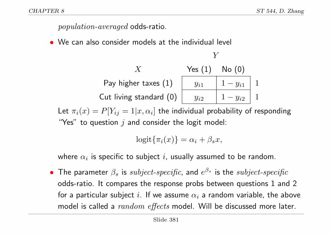
• We can also consider models at the individual level

Y

X Yes (1) No (0)

Pay higher taxes (1) yi1 1− yi1 1

Cut living standard (0) yi2 1− yi2 1

Let πi(x) = P [Yij = 1|x, αi] the individual probability of responding

“Yes” to question j and consider the logit model:

logit{πi(x)} = αi + βsx,

where αi is specific to subject i, usually assumed to be random.

• The parameter βs is subject-specific, and eβs is the subject-specific

odds-ratio. It compares the response probs between questions 1 and 2

for a particular subject i. If we assume αi a random variable, the above

model is called a random effects model. Will be discussed more later.

Slide 381


II.2 Conditional logistic regression for matched data from prospective

studies

• If we assume the subject-specific logit model for the opinion data

logit{πi(x)} = αi + βsx, i = 1, 2, · · · , n.

Since there are n many αi’s, we do not want to conduct the ML

analysis.

• Conditional approach: find out sufficient stat for αi’s and use the

conditional distribution of data given the suff. stat.

• It can be shown that the conditional likelihood of βs is

Lc(βs) =eβsn12

(1 + eβs)n21+n12

The conditional ML estimate: βs = log(n12/n21). The variance

estimate of βs can be shown to be 1/n12 + 1/n21.

Slide 382


• For our data, the subject-specific odds-ratio estimate is

eβs = n12/n21 = 132/107 = 1.23.

Note that this subject-specific odds-ratio estimate is greater than the

population-averaged odds-ratio estimate θXY = 1.11.

• SAS program and part of the output:proc logistic data=newdata descending;

class id;model y = x / link=logit;strata id;

run;

*******************************************************************

Analysis of Conditional Maximum Likelihood Estimates

Standard WaldParameter DF Estimate Error Chi-Square Pr > ChiSq

x 1 0.2100 0.1301 2.6055 0.1065

We can check that 0.21 = log(132/107), SE(βs) =√

1/132 + 1/107.

• Note: We can put more covariates in the conditional logistic

regression model to adjust their effects.

Slide 383


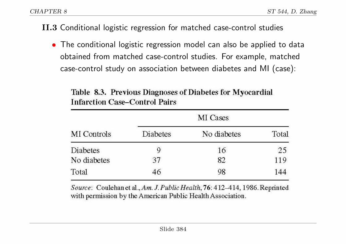
II.3 Conditional logistic regression for matched case-control studies

• The conditional logistic regression model can also be applied to data

obtained from matched case-control studies. For example, matched

case-control study on association between diabetes and MI (case):

Slide 384


• Let Yij = 1/0 for MI/control for subject j in pair i, x = 1/0 for

diabetes/no diabetes. There are 144 tables like the following:

Y

1 0

X 1 1 1

0 0 0

Type I: 9

1 0

0 1

1 0

III: 16

1 0

1 0

0 1

II: 37

1 0

0 0

1 1

IV: 82

• Treat data as if from a prospective study and fit

logit{P (Yij = 1} = αi + βsx, i = 1, 2, · · · , n pair, j = 1, 2.

• The conditional MLE of βs is

βs = log(n21/n12) = log(37/16) = 0.838 with variance estimate:

var(βs) = 1/37 + 1/16 = 0.09, SE(βs) =√

0.09 = 0.3

Slide 385


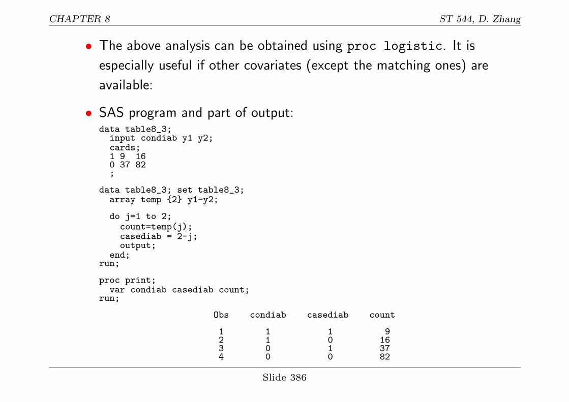
• The above analysis can be obtained using proc logistic. It is

especially useful if other covariates (except the matching ones) are

available:

• SAS program and part of output:data table8_3;

input condiab y1 y2;cards;1 9 160 37 82;


do j=1 to 2;count=temp(j);casediab = 2-j;output;

end;run;

proc print;var condiab casediab count;

run;

Obs condiab casediab count

1 1 1 92 1 0 163 0 1 374 0 0 82

Slide 386


title "Recover individual pair data";data newdata; set table8_3;

retain pair;if _n_=1 then pair=0;

do i=1 to count;pair = pair+1;do mi=0 to 1;

if mi=0 thendiab = condiab; /* for MI=0, the diab info is the control diab info */

elsediab = casediab; /* for MI=1, the diab info is the case diab info */

output;end;

end;run;

proc logistic descending;class pair;model mi = diab / link=logit;strata pair;

run;

*************************************************************************

Analysis of Conditional Maximum Likelihood Estimates


diab 1 0.8383 0.2992 7.8501 0.0051

Slide 387


II.4 Connection between McNemar test and CMH test

• The table given at the beginning can be viewed as a summary of 1144

partial 2× 2 tables, one for each subject:

Y

1 0

X 1 (Pay higher taxes) yi1 1− yi1 1

0 (Cut living standard) yi2 1− yi2 1

• There are only 4 types of such tables:

Y

1 0

X 1 1 0

0 1 0

Type I: n11

1 0

1 0

0 1

II: n12

1 0

0 1

1 0

III: n21

1 0

0 1

0 1

IV: n22

Slide 388


• Let us construct the CMH test for H0 : X and Y are conditional

independent given each subject:

E(yi1|margins, H0) =

1 for type I tables

1/2 for type II or III tables

0 for type IV tables

var(yi2|margins, H0) =

0 for type I or IV tables

1×1×122×(2−1) = 1

4 for type II or III tables

⇒

χ2CMH =

[n11(1− 1) + n12(1− 0.5) + n21(0− 0.5) + n22(0− 0)]2

n11 × 0 + n12 × 0.25 + n21 × 0.25 + n22 × 0

=(n12 − n21)2

n21 + n12,

the same as the McNemar’s test!

Slide 389


III Comparing Margins of Square Tables

III.1 Comparing margins for nominal response

• Example (Table 8.5) Coffee brand choice between 1st and 2nd

purchases:

Slide 390


• Let

Y1 = coffee brand choice at first purchase,

Y2 = coffee brand choice at second purchase.

We are interested in testing H0 : P [Y1 = k] = P [Y2 = k]

(k = 1, 2, 3, 4, 5).

• We can test the above H0 by comparing sample marginal proportions

pi+ to p+i:

d =

p1+ − p+1

p2+ − p+2

...

pI−1,+ − p+,I−1

Then construct

χ2 = dT {var(d)}−1dH0∼ χ2

I−1.

Slide 391


• We can conduct the above test using proc catmod.


input firstbuy y1-y5;cards;1 93 17 44 7 102 9 46 11 0 93 17 11 155 9 124 6 4 9 15 25 10 4 12 2 27;


do secbuy=1 to 5;count=temp(secbuy);output;

end;run;

proc print;var firstbuy secbuy count;

run;

Slide 392


Obs firstbuy secbuy count

1 1 1 932 1 2 173 1 3 444 1 4 75 1 5 106 2 1 97 2 2 468 2 3 119 2 4 0

10 2 5 911 3 1 1712 3 2 1113 3 3 15514 3 4 915 3 5 1216 4 1 617 4 2 418 4 3 919 4 4 1520 4 5 221 5 1 1022 5 2 423 5 3 1224 5 4 225 5 5 27

proc freq;weight count;tables firstbuy*secbuy / norow nocol;test agree;

run;

Slide 393


Table of firstbuy by secbuy

firstbuy secbuy

Frequency|Percent | 1| 2| 3| 4| 5| Total---------+--------+--------+--------+--------+--------+

1 | 93 | 17 | 44 | 7 | 10 | 171| 17.19 | 3.14 | 8.13 | 1.29 | 1.85 | 31.61

---------+--------+--------+--------+--------+--------+2 | 9 | 46 | 11 | 0 | 9 | 75

| 1.66 | 8.50 | 2.03 | 0.00 | 1.66 | 13.86---------+--------+--------+--------+--------+--------+

3 | 17 | 11 | 155 | 9 | 12 | 204| 3.14 | 2.03 | 28.65 | 1.66 | 2.22 | 37.71

---------+--------+--------+--------+--------+--------+4 | 6 | 4 | 9 | 15 | 2 | 36

| 1.11 | 0.74 | 1.66 | 2.77 | 0.37 | 6.65---------+--------+--------+--------+--------+--------+

5 | 10 | 4 | 12 | 2 | 27 | 55| 1.85 | 0.74 | 2.22 | 0.37 | 4.99 | 10.17

---------+--------+--------+--------+--------+--------+Total 135 82 231 33 60 541

24.95 15.16 42.70 6.10 11.09 100.00

Statistics for Table of firstbuy by secbuy

Test of Symmetry------------------------Statistic (S) 20.4124DF 10Pr > S 0.0256

Slide 394


proc catmod data=table8_5;;weight count;response marginals;model firstbuy*secbuy = _response_;repeated time 2;

run;

****************************************************************

Analysis of Variance

Source DF Chi-Square Pr > ChiSq--------------------------------------------Intercept 4 6471.41 <.0001time 4 12.58 0.0135

The Wald test for marginal homogeneity is χ2 = 12.6 with df = 4,

p-value=0.0135. We reject the marginal homogeneity at level 0.05.

That is, we conclude that customers’ coffee brand choices between

their first and second buys are not the same.

Slide 395


III.2 Comparing margins for ordinal response

• Example (Table 8.6): Response to recycling and driving less to help

environment

• Let Yi1 be the subject i’s response to “How often do you make a

special effort to sort ...”, Yi2 be the subject i’s response to “How often

do you cut back on driving ...”.

Slide 396


• Use 1, 2, 3, 4 for four values: never/sometimes/often/always and

consider cumulative logit model:

logit{P [Yi1 ≥ j]} = αj + β,

logit{P [Yi2 ≥ j]} = αj .

Then H0 : β = 0 ⇒ marginal homogeneity.

• We can fit the above model using proc genmod by taking into

account the correlation between 2 obs from the same subject using

GEE (this analysis is different from the one given in the textbook).


input recycle y1-y4;cards;4 12 43 163 2333 4 21 99 1852 4 8 77 2301 0 1 18 132;

Slide 397



do j=1 to 4;driveles=5-j;count=temp(j);output;

end;run;

proc print;var recycle driveles count;

run;

Obs recycle driveles count

1 4 4 122 4 3 433 4 2 1634 4 1 2335 3 4 46 3 3 217 3 2 998 3 1 1859 2 4 4

10 2 3 811 2 2 7712 2 1 23013 1 4 014 1 3 115 1 2 1816 1 1 132

Slide 398


title "Recover individual data";data newdata; set table8_6;

retain id;if _n_=1 then id=0;

do i=1 to count;id = id+1;do question=1 to 2;

x = 2-question;if question=1 then y=recycle;if question=2 then y=driveles;output;

end;end;

run;

proc genmod data=newdata descending;class id;model y = x / dist=multinomial link=clogit;repeated subject=id / type=ind;

run;

Slide 399


Response Profile

Ordered TotalValue y Frequency

1 4 4712 3 3823 2 6764 1 931

PROC GENMOD is modeling the probabilities of levels of y having LOWER OrderedValues in the response profile table.



Intercept1 -3.3511 0.0829 -3.5136 -3.1886 -40.43 <.0001Intercept2 -2.2767 0.0743 -2.4224 -2.1311 -30.64 <.0001Intercept3 -0.5849 0.0588 -0.7002 -0.4696 -9.94 <.0001x 2.7536 0.0815 2.5939 2.9133 33.80 <.0001

The Wald test for H0 : β = 0 is z = 33.80, p-value< 0.0001. Since

β > 0, people are willing to put more effort in recycling than driving

less to help environment.

Slide 400


IV Symmetry and Quasi-Symmetry for Square Tables

IV.1 Symmetry for nominal square tables

• Suppose Y1, Y2 are 2 categorical variables taking the same values

1, 2, · · · , I with the probability structure as (assuming I = 3):

Y2

1 2 3

1 π11 π12 π13

Y1 2 π21 π22 π23

3 π31 π32 π33

We are interested in testing H0 : πij = πji.

• Given data {nij} from a multinomial sampling, the MLE’s of πij under

H0 are:

πii = nii/n, πij = (nij + nji)/(2n).

Slide 401


• The Pearson χ2 test and LRT for H0 : πij = πji are

χ2(S) =∑i<j

(nij − nji)2

nij + nji

H0∼ χ2df

G2(S) = 2∑i<j

nij log(2nij/(nij + nji)) + nji log(2nji/(nij + nji))H0∼ χ2

df

with df = I(I − 1)/2.

• The above Pearson χ2 test is an extension of the McNemar’s test.

• For the coffee data, χ2 = 20.4, G2 = 22.5 with df = 5(5− 1)/2 = 10.

The Pearson χ2 = 20.4 can be obtained using test agree in proc

freq.

Slide 402


IV.2 Quasi-symmetry for nominal square tables

• The symmetry (⇒marginal homogeneity) model seldom fits data well.

A more general model is the quasi-symmetry model that allows

marginal heterogeneity:

log(πij/πji) = βi − βj (i < j).

Of course, only I − 1 many βi’s are needed. We can set βI = 0.

• If βi = 0 (i = 1, 2, ..., I − 1), then we have a marginal symmetry model.

• The fitting of the above model can be realized by fitting a logistic

model to the paired data (nij , nji) (i < j) treating nij as the total #

of success and nji as the total number of failure with no intercept.

• We need to delete the diagonal elements nii’s.

Slide 403


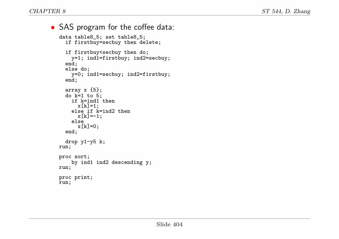
• SAS program for the coffee data:data table8_5; set table8_5;

if firstbuy=secbuy then delete;

if firstbuy<secbuy then do;y=1; ind1=firstbuy; ind2=secbuy;

end;else do;

y=0; ind1=secbuy; ind2=firstbuy;end;

array x {5};do k=1 to 5;

if k=ind1 thenx[k]=1;

else if k=ind2 thenx[k]=-1;

elsex[k]=0;

end;

drop y1-y5 k;run;

proc sort;by ind1 ind2 descending y;

run;

proc print;run;

Slide 404


Obs firstbuy secbuy count y ind1 ind2 x1 x2 x3 x4 x5

1 1 2 17 1 1 2 1 -1 0 0 02 2 1 9 0 1 2 1 -1 0 0 03 1 3 44 1 1 3 1 0 -1 0 04 3 1 17 0 1 3 1 0 -1 0 05 1 4 7 1 1 4 1 0 0 -1 06 4 1 6 0 1 4 1 0 0 -1 07 1 5 10 1 1 5 1 0 0 0 -18 5 1 10 0 1 5 1 0 0 0 -19 2 3 11 1 2 3 0 1 -1 0 0

10 3 2 11 0 2 3 0 1 -1 0 011 2 4 0 1 2 4 0 1 0 -1 012 4 2 4 0 2 4 0 1 0 -1 013 2 5 9 1 2 5 0 1 0 0 -114 5 2 4 0 2 5 0 1 0 0 -115 3 4 9 1 3 4 0 0 1 -1 016 4 3 9 0 3 4 0 0 1 -1 017 3 5 12 1 3 5 0 0 1 0 -118 5 3 12 0 3 5 0 0 1 0 -119 4 5 2 1 4 5 0 0 0 1 -120 5 4 2 0 4 5 0 0 0 1 -1

Slide 405


title "Quasi-symmetry model";proc genmod descending;

freq count;model y = x1 x2 x3 x4 / dist=bin link=logit aggregate noint;

run;

*************************************************************************

Criteria For Assessing Goodness Of Fit

Criterion DF Value Value/DF

Deviance 6 9.9740 1.6623Scaled Deviance 6 9.9740 1.6623Pearson Chi-Square 6 8.5303 1.4217Scaled Pearson X2 6 8.5303 1.4217

Analysis Of Maximum Likelihood Parameter Estimates

Standard Wald 95% WaldParameter DF Estimate Error Confidence Limits Chi-Square Pr > ChiSq

Intercept 0 0.0000 0.0000 0.0000 0.0000 . .x1 1 0.5954 0.2937 0.0199 1.1710 4.11 0.0426x2 1 -0.0040 0.3294 -0.6495 0.6415 0.00 0.9903x3 1 -0.1133 0.2851 -0.6720 0.4455 0.16 0.6911x4 1 0.3021 0.4016 -0.4850 1.0892 0.57 0.4519Scale 0 1.0000 0.0000 1.0000 1.0000

• Note: There is a weight statement in proc genmod. But it is not for

the count nij ’s!

Slide 406


• We can also use Proc Logistic to fit the above model and get a test

of symmetry under the Quasi-symmetry model.title "Quasi-symmetry model using proc logistic";proc logistic descending;

freq count;model y = x1 x2 x3 x4 / link=logit noint;

run;

*************************************************************************

Testing Global Null Hypothesis: BETA=0

Test Chi-Square DF Pr > ChiSq

Likelihood Ratio 12.4989 4 0.0140Score 12.2913 4 0.0153Wald 11.8742 4 0.0183

Analysis of Maximum Likelihood Estimates


x1 1 0.5954 0.2937 4.1105 0.0426x2 1 -0.00401 0.3294 0.0001 0.9903x3 1 -0.1133 0.2851 0.1579 0.6911x4 1 0.3021 0.4016 0.5659 0.4519

Slide 407


• From the output, we know that the GOF stats:

χ2(QS) = 8.5, G2(QS) = 10.0,

with df = 6. Reasonably good fit.

• We know the GOF for symmetry model

χ2(S) = 20.4, G2(S) = 22.5,

with df = 10.

• Assuming quasi-symmetry model, symmetry model can be tested

using LRT

LRT = 22.5− 10.0 = 12.5,

with df = 10− 6 = 4, ⇒ Reject symmetry model under

quasi-symmetry model.

Slide 408


IV.3 Quasi-symmetry for ordinal square tables

• For square tables formed with two ordinal variables with the same

levels, we can assign scores ui to the ith level and consider the

following ordinal quasi-symmetry model:

log(πij/πji) = β(uj − ui), (i < j).

• Similar to the quasi-symmetry model for nominal square tables, we

can fit the above model by fitting a logistic model to the paired data

(nij , nji) (i < j) treating nij as the total # of success and nji as the

total number of failure and x = uj − ui as the covariate with no

intercept.

• We need to delete the diagonal elements nii’s.

• β = 0 ⇒ symmetry. So we can test H0 : β = 0 to test symmetry.

Slide 409


• Let us use the recycle example to illustrate this above model. SAS

program and part of output:data table8_6; set table8_6;

if recycle=driveles then delete;

if recycle>driveles then do;y=1;x=recycle-driveles;ind1=driveles;ind2=recycle;

end;else do;

y=0;x=driveles-recycle;ind1=recycle;ind2=driveles;

end;

array z {4};do k=1 to 4;

if k=ind1 thenz[k]=1;

else if k=ind2 thenz[k]=-1;

elsez[k]=0;

end;run;

Slide 410


title "Ordinal quasi-symmetry model";proc logistic data=table8_6;

freq count;model y (ref="0") = x / link=glogit aggregate scale=none noint;

run;

**********************************************************************

Deviance and Pearson Goodness-of-Fit Statistics

Criterion Value DF Value/DF Pr > ChiSq

Deviance 2.0309 2 1.0155 0.3622Pearson 2.1029 2 1.0514 0.3494

Testing Global Null Hypothesis: BETA=0

Test Chi-Square DF Pr > ChiSq

Likelihood Ratio 1101.7102 1 <.0001Score 762.6001 1 <.0001Wald 252.0238 1 <.0001

Analysis of Maximum Likelihood Estimates

Standard WaldParameter y DF Estimate Error Chi-Square Pr > ChiSq

x 1 1 2.3936 0.1508 252.0238 <.0001

• GOF: Pearson χ2 = 2.1, G2 = 2.0 with df = 2. Good fit. Based on

this model, reject H0 : β = 0, so reject symmetry.

Slide 411


• From the output, we got

log(π12/π21) = 2.3936(2− 1) = 2.3936

log(π13/π31) = 2.3936(3− 1) = 4.78

log(π14/π41) = 2.3936(4− 1) = 7.18

log(π23/π32) = 2.3936(3− 2) = 2.3936

log(π24/π42) = 2.3936(4− 2) = 4.78

log(π34/π43) = 2.3936

For example,

π12 = π21e2.3936 = 11π21

That is,

P[Recycle=Always, Drive-less=often]=11 × P[Recycle=Often,

Drive-less=Always]

Slide 412


title "Quasi-symmetry model treating ordinal as nominal";proc genmod data=table8_6 descending;

freq count;model y = z1 z2 z3 / dist=bin link=logit aggregate noint;

run;

************************************************************************






Intercept 0 0.0000 0.0000 0.0000 0.0000 . .z1 1 6.9269 0.4708 6.0040 7.8497 216.43 <.0001z2 1 4.3452 0.4223 3.5175 5.1729 105.87 <.0001z3 1 1.9937 0.3822 1.2447 2.7428 27.22 <.0001Scale 0 1.0000 0.0000 1.0000 1.0000

• Treating table as a nominal table, the quasi-symmetry has GOF:

Pearson χ2 = 2.68, G2 = 2.71 with df = 3, again reasonably good fit.

Slide 413


• From nominal quasi-symmetry model fit, we know that

log(π12/π21) = 6.9269− 4.3452 = 2.58

log(π13/π31) = 6.9269− 1.9937 = 4.93

log(π14/π41) = 6.9269

log(π23/π32) = 4.3452− 1.9937 = 2.35

log(π24/π42) = 4.3452

log(π34/π43) = 1.9937

Very similar to the results from the ordinal quasi-symmetry model fit.

• Note: Pearson GOF and LRT for symmetry: χ2 = 856, G2 = 1093,

df = 6. Very poor fit!

Slide 414


V Analyzing Rater Agreement

• Example (Table 8.7): Diagnoses of carcinoma by two pathologists

Slide 415


• Usually, the diagnoses (Y1, Y2) between two raters are correlated (not

independent). So if we use Pearson χ2 or LRT G2, we would reject

independence. Indeed,

χ2 = 120, G2 = 118, df = 9,

even without taking into the ordinal scale. See the program and output

on the next slide.

• However, (Y1, Y2) being dependent does not mean Y1 agrees well with

Y2. That is, association is not the same as agreement.

• Pearson χ2 for symmetry H0 : πij = πji is χ2 = 30.3 with df = 6.

Symmetry model not good either!

• We may consider models that captures agreement and disagreement.

Slide 416


data table8_7;input rater1 y1-y4;cards;1 22 2 2 02 5 7 14 03 0 2 36 04 0 1 17 10;

data table8_7; set table8_7;array temp {4} y1-y4;do rater2=1 to 4;

count=temp(rater2);output;

end;run;

proc freq;weight count;tables rater1*rater2 / norow nocol chisq;test agree;

run;

*************************************************************************Statistics for Table of rater1 by rater2

Statistic DF Value Prob------------------------------------------------------Chi-Square 9 120.2635 <.0001Likelihood Ratio Chi-Square 9 117.9569 <.0001Mantel-Haenszel Chi-Square 1 73.4843 <.0001

Test of Symmetry------------------------Statistic (S) 30.2857DF 6Pr > S <.0001

Slide 417


Simple Kappa Coefficient--------------------------------Kappa 0.4930ASE 0.056795% Lower Conf Limit 0.381895% Upper Conf Limit 0.6042

Test of H0: Kappa = 0

ASE under H0 0.0501Z 9.8329One-sided Pr > Z <.0001Two-sided Pr > |Z| <.0001

Weighted Kappa Coefficient--------------------------------Weighted Kappa 0.6488ASE 0.047795% Lower Conf Limit 0.555495% Upper Conf Limit 0.7422

Test of H0: Weighted Kappa = 0

ASE under H0 0.0631Z 10.2891One-sided Pr > Z <.0001Two-sided Pr > |Z| <.0001

Sample Size = 118

Slide 418


V.1 Quasi-independence model for rater agreement

• Treat {nij}’s as independent Poisson data with mean µij ’s, we can fit

the following quasi-independence model to the agreement data:

logµij = λ+ λXi + λYj + δiI(i = j).

• Note: Without δi, the above model reduces to the independence

model between Y1 and Y2. So the name quasi-independence model.

• Interpretation of quasi-independence model: For a pair of subjects,

consider the event that each rater put one subject in category a and

the other subject in category b. Then the conditional odds that two

raters agree rather than disagree on which subject is cat a and which

one in cat b is

τab =πaaπbbπabπba

= eδa+δb .

So if δi > 0, then two raters tend to agree rather than disagree.

Slide 419


• SAS program and output for the quasi-independence model:data table8_7; set table8_7;

if rater1=rater2 thenqi=rater1;

elseqi=5;

run;

title "Quasi-independence model";proc genmod data=table8_7;

class rater1 rater2 qi;model count = rater1 rater2 qi / dist=poi link=log;

run;

************************************************************************






qi 1 1 3.8611 0.7297 2.4308 5.2913 28.00 <.0001qi 2 1 0.6042 0.6900 -0.7481 1.9566 0.77 0.3812qi 3 1 1.9025 0.8367 0.2625 3.5425 5.17 0.0230qi 4 0 25.3775 0.0000 25.3775 25.3775 . .qi 5 0 0.0000 0.0000 0.0000 0.0000 . .Scale 0 1.0000 0.0000 1.0000 1.0000

Slide 420


• The GOF stats of the above model are

χ2 = 11.5, G2 = 13.2, df = 5.

Not a good fit!

• If we assume the model, then δ1 = 3.86, δ2 = 0.60, δ3 = 1.90. All are

positive. So two raters agree more than disagree.

• Consider the event that each rater put one subject in category 2 and

the other subject in category 3, then the conditional odds that raters

agree rather than disagree is

τ23 = eδ2+δ3 = e0.60+1.90 = 12.3.

Slide 421


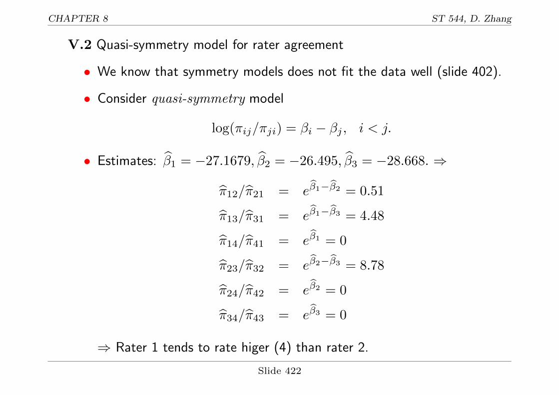
V.2 Quasi-symmetry model for rater agreement

• We know that symmetry models does not fit the data well (slide 402).

• Consider quasi-symmetry model

log(πij/πji) = βi − βj , i < j.

• Estimates: β1 = −27.1679, β2 = −26.495, β3 = −28.668. ⇒

π12/π21 = eβ1−β2 = 0.51

π13/π31 = eβ1−β3 = 4.48

π14/π41 = eβ1 = 0

π23/π32 = eβ2−β3 = 8.78

π24/π42 = eβ2 = 0

π34/π43 = eβ3 = 0

⇒ Rater 1 tends to rate higer (4) than rater 2.

Slide 422


• SAS program and part of output:data table8_7; set table8_7;

if rater1=rater2 then delete;

if rater1<rater2 then y=1;else y=0;

if rater1<rater2 then do;ind1=rater1; ind2=rater2;

end;else do;

ind1=rater2; ind2=rater1;end;




elsex[k]=0;

end;drop y1-y4 k;

run;


run;

proc print;run;

Slide 423


Obs rater1 rater2 count qi y ind1 ind2 x1 x2 x3 x4

1 1 2 2 5 1 1 2 1 -1 0 02 2 1 5 5 0 1 2 1 -1 0 03 1 3 2 5 1 1 3 1 0 -1 04 3 1 0 5 0 1 3 1 0 -1 05 1 4 0 5 1 1 4 1 0 0 -16 4 1 0 5 0 1 4 1 0 0 -17 2 3 14 5 1 2 3 0 1 -1 08 3 2 2 5 0 2 3 0 1 -1 09 2 4 0 5 1 2 4 0 1 0 -1

10 4 2 1 5 0 2 4 0 1 0 -111 3 4 0 5 1 3 4 0 0 1 -112 4 3 17 5 0 3 4 0 0 1 -1

Slide 424


title "Quasi-symmetry model";proc genmod descending;

freq count;model y = x1 x2 x3 / dist=bin link=logit aggregate noint;

run;






Intercept 0 0.0000 0.0000 0.0000 0.0000 . .x1 1 -27.1679 0.9731 -29.0752 -25.2606 779.42 <.0001x2 1 -26.4950 0.7628 -27.9900 -24.9999 1206.44 <.0001x3 0 -28.6680 0.0000 -28.6680 -28.6680 . .Scale 0 1.0000 0.0000 1.0000 1.0000

• GOF: Pearson χ2 = 0.63, Deviance G2 = 0.98, df = 2, good fit.

Slide 425


V.3 Kappa measure of rater agreement

• Cohen’s Kappa:

κ =

∑πii −

∑πi+π+i

1−∑πi+π+i

.

The numerator = agreement probabilities - agreement expected under

independence.

The denominator = maximum difference.

• Perfect agreement ⇔ κ = 1

Random agreement ⇔ κ = 0.

• Replacing πij ’s by the sample proportions pij ’s leads to an estimate of

κ.

• For ordinal tables, using scores to emphasizes the disagreement ⇒weighted κ.

• Software: Statement test agree in proc freq. Slides 417-418.

Slide 426


VI Bradley-Terry Model for Paired Preferences

• Example:

Slide 427


• Let

Πij = P [Player i wins Player j].

Consider Bradley-Terry model for comparison:

log{Πij/(1−Πij)} = log{Πij/Πji} = βi − βj , i < j = 1, ..., I.

Need to set βI = 0.

• We can rank players based on βi’s.

• The above model can be fit by treating it as a quasi-symmetry model.

Slide 428


data table8_9;input winner player $ y1-y5;cards;1 Agassi . 0 0 1 12 Federer 6 . 3 9 53 Henman 0 1 . 0 14 Hewitt 0 0 2 . 35 Roddick 0 0 1 2 .;

data table8_9; set table8_9;array temp {5} y1-y5;do loser=1 to 5;

count=temp(loser);output;

end;run;

data table8_9; set table8_9;if winner=loser then delete;if winner<loser then do;

y=1; ind1=winner; ind2=loser;end;else do ;

y=0; ind1=loser; ind2=winner;end;




elsex[k]=0;

end;drop y1-y5 k;

run;

Slide 429



run;

proc print;run;

**************************************************************************

Obs winner player loser count y ind1 ind2 x1 x2 x3 x4 x5

1 1 Agassi 2 0 1 1 2 1 -1 0 0 02 2 Federer 1 6 0 1 2 1 -1 0 0 03 1 Agassi 3 0 1 1 3 1 0 -1 0 04 3 Henman 1 0 0 1 3 1 0 -1 0 05 1 Agassi 4 1 1 1 4 1 0 0 -1 06 4 Hewitt 1 0 0 1 4 1 0 0 -1 07 1 Agassi 5 1 1 1 5 1 0 0 0 -18 5 Roddick 1 0 0 1 5 1 0 0 0 -19 2 Federer 3 3 1 2 3 0 1 -1 0 0

10 3 Henman 2 1 0 2 3 0 1 -1 0 011 2 Federer 4 9 1 2 4 0 1 0 -1 012 4 Hewitt 2 0 0 2 4 0 1 0 -1 013 2 Federer 5 5 1 2 5 0 1 0 0 -114 5 Roddick 2 0 0 2 5 0 1 0 0 -115 3 Henman 4 0 1 3 4 0 0 1 -1 016 4 Hewitt 3 2 0 3 4 0 0 1 -1 017 3 Henman 5 1 1 3 5 0 0 1 0 -118 5 Roddick 3 1 0 3 5 0 0 1 0 -119 4 Hewitt 5 3 1 4 5 0 0 0 1 -120 5 Roddick 4 2 0 4 5 0 0 0 1 -1

Slide 430


title "Bradley-Terry Model for Tennis Matches";proc genmod descending;

freq count;model y = x1 x2 x3 x4 / dist=bin link=logit aggregate noint covb;

run;

************************************************************************Criteria For Assessing Goodness Of Fit



Estimated Covariance Matrix

Prm2 Prm3 Prm4 Prm5

Prm2 1.93092 1.06655 0.27405 0.40015Prm3 1.06655 1.73340 0.34535 0.42773Prm4 0.27405 0.34535 1.10898 0.32444Prm5 0.40015 0.42773 0.32444 0.63787



Intercept 0 0.0000 0.0000 0.0000 0.0000 . .x1 1 1.4489 1.3896 -1.2747 4.1724 1.09 0.2971x2 1 3.8815 1.3166 1.3011 6.4620 8.69 0.0032x3 1 0.1875 1.0531 -1.8765 2.2515 0.03 0.8587x4 1 0.5734 0.7987 -0.9920 2.1387 0.52 0.4728Scale 0 1.0000 0.0000 1.0000 1.0000

Slide 431


• The GOF: χ2 = 11.6, Deviance G2 = 8.2 with df = 5. Not a very

good fit.

• Estimates of βi’s:

β1 = 1.45, β2 = 3.88, β3 = 0.19, β4 = 0.57, β5 = 0 .

⇒

β2 > β1 > β4 > β3 > β5.

The Ranking: Federer, Agassi, Hewitt, Henman, Roddick.

Slide 432


• We can estimate the winning probability that Player i wins against

Player j Πij :

Πij =eβi−βj

1 + eβi−βj

.

For example, consider Federer v.s. Agassi:

Π21 =eβ2−β1

1 + eβ2−β1

=e3.88−1.45

1 + e3.88−1.45= 0.92.

var(β2 − β1) = var(β2) + var(β1)− 2cov(β2, β1)

= 1.73340 + 1.93092− 2× 1.06655 = 1.5312

SE(β2 − β1) = 1.24

A 95% CI for β2 − β1:

β2 − β1 ± 1.96SE(β2 − β1) = 2.43± 1.96× 1.24 = [0, 4.86].

Slide 433


A 95% CI for Π21:

[e0

1 + e0,

e4.86

1 + e4.86] = [0.5, 0.99].

• Note: We can estimate Πij based on the model even though Player i

may not have played Player j. For example, Agassi (Player 1) and

Henman (Player 3) did not play in 2004-2005. But we can estimate

the winning probability for Agassi v.s. Henman Π13.

• Note: The above model can also be applied to other settings such as

wine tasting.

Slide 434

Documents

CHAPTER 8 ST 544, D. Zhang 8 Models for Matched Pairs