1

Objective

Compare of two matched-paired means using two samples from each population.

Hypothesis Tests and Confidence Intervals of two dependent means use the t-distribution

Section 9.4Inferences About Two Means

(Matched Pairs)

2

Definition

Two samples are dependent if there is some relationship between the two samples so that each value in one sample is paired with a corresponding value in the other sample.

Two samples can be treated as the matched pairs of values.

3

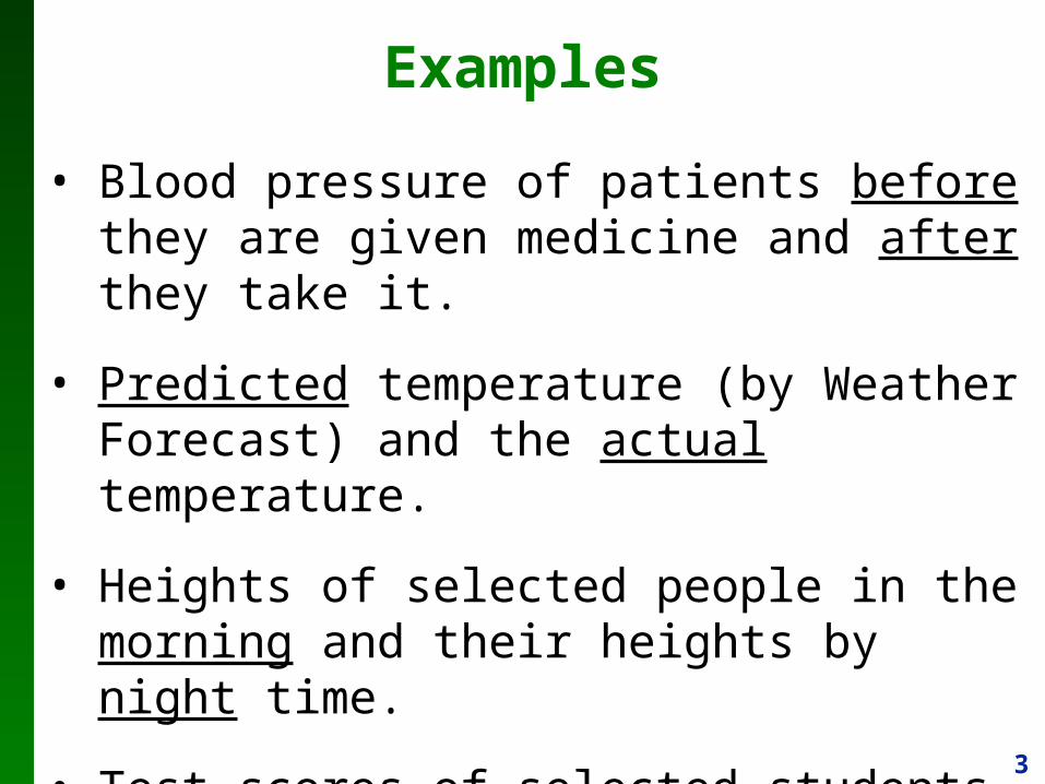
Examples

• Blood pressure of patients before they are given medicine and after they take it.

• Predicted temperature (by Weather Forecast) and the actual temperature.

• Heights of selected people in the morning and their heights by night time.

• Test scores of selected students in Calculus-I and their scores in Calculus-II.

4

Example 1

First sample: weights of 5 students in April

Second sample: their weights in September

These weights make 5 matched pairs

Third line: differences between April weights and September weights (net change in weight for each student, separately)

In our calculations we only use differences (d), not the values in the two samples.

5

Notation

d Individual difference between two matched paired values

μd Population mean for the difference of the two values.

n Number of paired values in sample

d Mean value of the differences in sample

sd Standard deviation of differences in sample

6

(1) The sample data are dependent (i.e. they make matched pairs)

(2) Either or both the following holds:

The number of matched pairs is large (n>30) orThe differences have a normal distribution

Requirements

All requirements must be satisfied to make a Hypothesis Test or to find a Confidence Interval

7

Tests for Two Dependent Means

Goal: Compare the mean of the differences

H0 : μd =

0

H1 : μd ≠ 0

Two tailed Left tailed Right tailed

H0 : μd =

0

H1 : μd < 0

H0 : μd =

0

H1 : μd > 0

8

t = d – µdsdn

degrees of freedom: df = n – 1

Note: d

= 0 according to H0

Finding the Test Statistic

9

Test Statistic

Note: Hypothesis Tests are done in same way as in Ch.8-5

Degrees of freedom df = n – 1

10

Steps for Performing a Hypothesis Test on Two Independent Means

• Write what we know

• State H0 and H1

• Draw a diagram

• Calculate the Sample Stats

• Find the Test Statistic

• Find the Critical Value(s)

• State the Initial Conclusion and Final Conclusion

Note: Same process as in Chapter 8

11

Example 1

Assume the differences in weight form a normal distribution.

Use a 0.05 significance level to test the claim that for the population of students, the mean change in weight from September to April is 0 kg (i.e. on average, there is no change)

Claim: μd = 0 using α = 0.05

12

H0 : µd = 0

H1 : µd ≠ 0t = 0.186

tα/2 = 2.78

t-dist.df = 4

Test Statistic

Critical Value

Initial Conclusion: Since t is not in the critical region, accept H0

Final Conclusion: We accept the claim that mean change in weight from

September to April is 0 kg.

-tα/2 = -2.78

Example 1

tα/2 = t0.025 = 2.78 (Using StatCrunch, df = 4)

d Data: -1 -1 4 -2 1

Sample Stats

n = 5 d = 0.2 sd = 2.387

Use StatCrunch: Stat – Summary Stats – Columns

Two-TailedH0 = Claim

13

H0 : µd = 0

H1 : µd ≠ 0Two-TailedH0 = Claim

Initial Conclusion: Since P-value is greater than α (0.05), accept H0

Final Conclusion: We accept the claim that mean change in weight from

September to April is 0 kg.

Example 1 d Data: -1 -1 4 -2 1Sample Stats

n = 5 d = 0.2 sd = 2.387

Use StatCrunch: Stat – Summary Stats – Columns

Null: proportion=

Alternative

Sample mean:

Sample std. dev.:

Sample size:

● Hypothesis Test0.2

2.387

5

0

≠

P-value = 0.8605

Stat → T statistics→ One sample → With summary

14

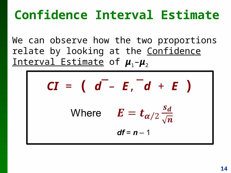
Confidence Interval Estimate

We can observe how the two proportions relate by looking at the Confidence Interval Estimate of μ1–μ2

CI = ( d – E, d + E )

15

Example 2 Find the 95% Confidence Interval Estimate of μd from the data in Example 1

Sample Stats

n = 5 d = 0.2 sd = 2.387

CI = (-2.8, 3.2)

tα/2 = t0.025 = 2.78 (Using StatCrunch, df = 4)

16

Example 2 Find the 95% Confidence Interval Estimate of μd from the data in Example 1

Sample Stats

n = 5 d = 0.2 sd = 2.387

Level:Sample mean:

Sample std. dev.:

Sample size:

● Confidence Interval0.2

2.387

5

0.95

Stat → T statistics→ One sample → With summary

CI = (-2.8, 3.2)