Chapter 8: Regression

Self-test answers

SELF-TEST Residuals are used to compute which of the three sums of squares?

The residuals are used to calculate the residual sum of squares (SSR). This value is calculated by first squaring the residuals and then adding them up.

SELF-TEST Once you have read Section 8.4, run a regression first with all the cases included and then with case 30 deleted.

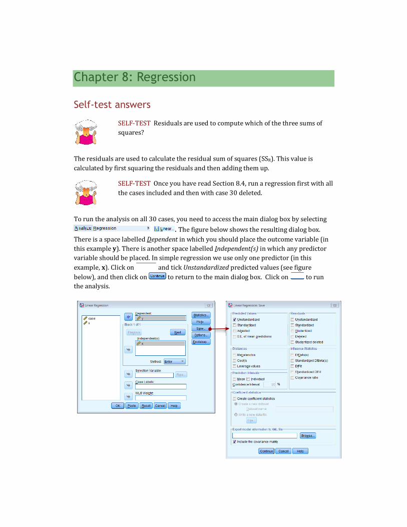
To run the analysis on all 30 cases, you need to access the main dialog box by selecting . The figure below shows the resulting dialog box.

There is a space labelled Dependent in which you should place the outcome variable (in this example y). There is another space labelled Independent(s) in which any predictor variable should be placed. In simple regression we use only one predictor (in this example, x). Click on and tick Unstandardized predicted values (see figure below), and then click on to return to the main dialog box. Click on to run the analysis.

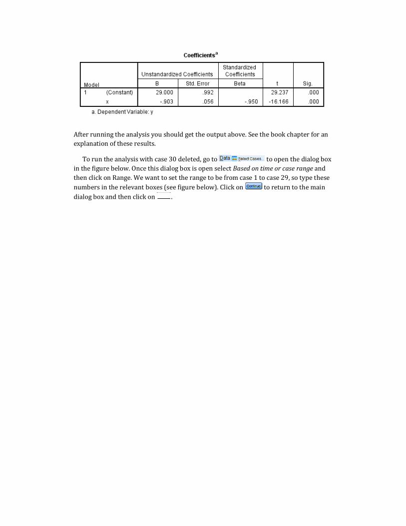
After running the analysis you should get the output above. See the book chapter for an explanation of these results.

To run the analysis with case 30 deleted, go to to open the dialog box in the figure below. Once this dialog box is open select Based on time or case range and then click on Range. We want to set the range to be from case 1 to case 29, so type these numbers in the relevant boxes (see figure below). Click on to return to the main dialog box and then click on .

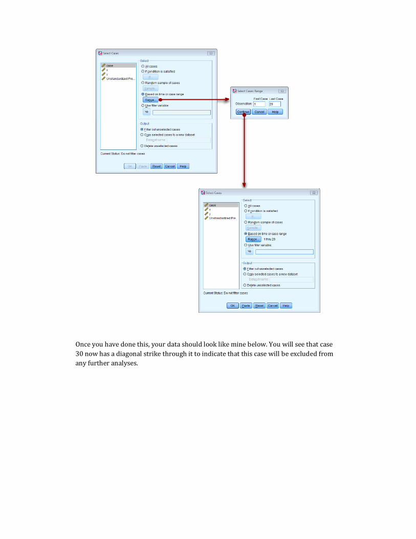
Once you have done this, your data should look like mine below. You will see that case 30 now has a diagonal strike through it to indicate that this case will be excluded from any further analyses.

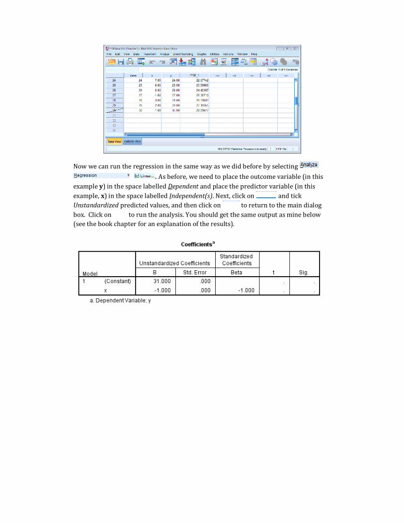
Now we can run the regression in the same way as we did before by selecting . As before, we need to place the outcome variable (in this

example y) in the space labelled Dependent and place the predictor variable (in this example, x) in the space labelled Independent(s). Next, click on and tick Unstandardized predicted values, and then click on to return to the main dialog box. Click on to run the analysis. You should get the same output as mine below (see the book chapter for an explanation of the results).

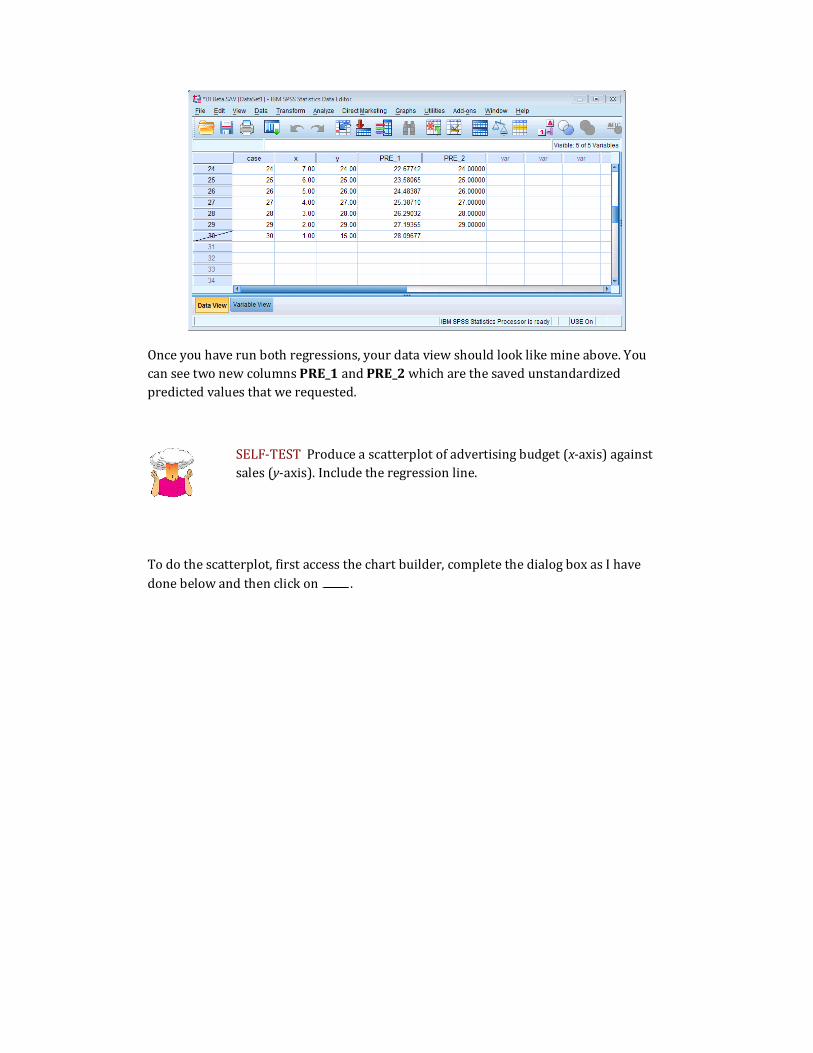
Once you have run both regressions, your data view should look like mine above. You can see two new columns PRE_1 and PRE_2 which are the saved unstandardized predicted values that we requested.

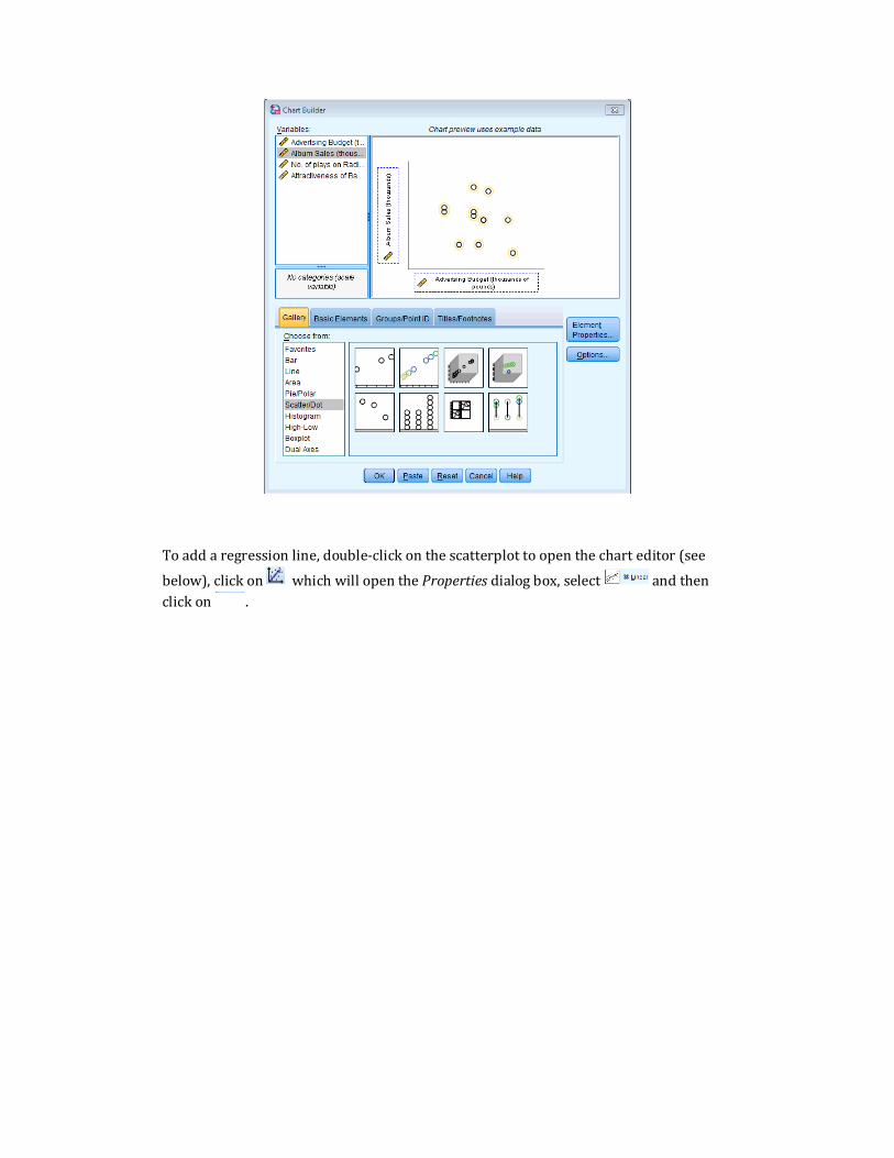
SELF-TEST Produce a scatterplot of advertising budget (x-axis) against sales (y-axis). Include the regression line.

To do the scatterplot, first access the chart builder, complete the dialog box as I have done below and then click on .

To add a regression line, double-click on the scatterplot to open the chart editor (see

below), click on which will open the Properties dialog box, select and then click on .

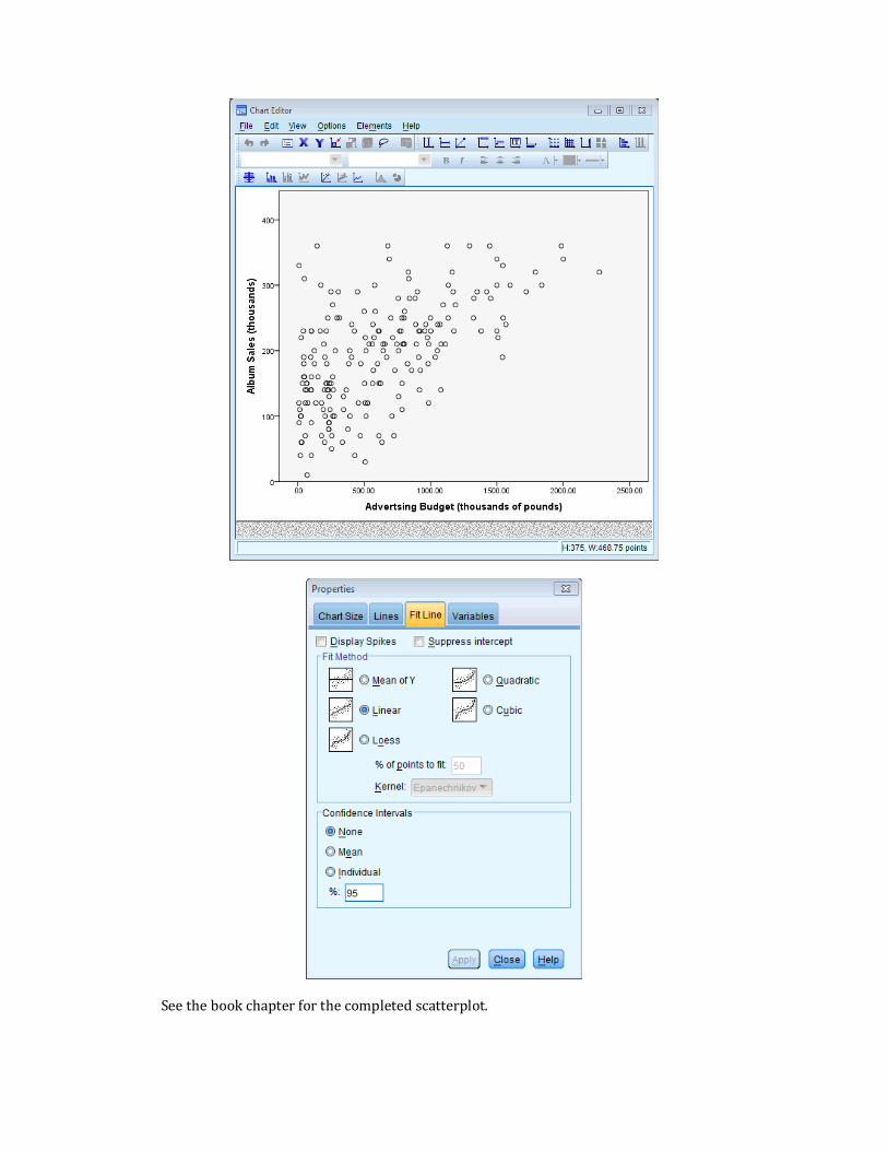
See the book chapter for the completed scatterplot.

SELF-TEST How is the t in Output 8.3 calculated? Use the values in the table to see if you can get the same value as SPSS.

It is calculated using this equation:

����������� � ���������

���

����������

���

Using the values from SPSS Output 8.3 to calculate t for the constant (t = 134.140/7.537 = 17.79), for the advertising budget, we get: 0.096/0.01 = 9.6. This value is different than the one in the output (t = 9.979) because SPSS rounds values in the output to three decimal places, but calculates t using unrounded values (usually this doesn’t make too much difference, but in this case it does!). In this case the rounding has had quite an effect on the standard error (its value is 0.009632 but it has been rounded to 0.01). To obtain the unrounded values, double-click the table in the SPSS output and then double-click the value that you wish to see in full. You should find that t = 0.096124/0.009632 = 9.979.

SELF-TEST How many records would be sold if we spent £666,000 on advertising the latest CD by black metal band Abgott?

He would sell 198,080 CDs:

albumsales� � 134.14 � �0.096 � advertisingbudget�� �134.14 � �0.096 � 666�� 198.08

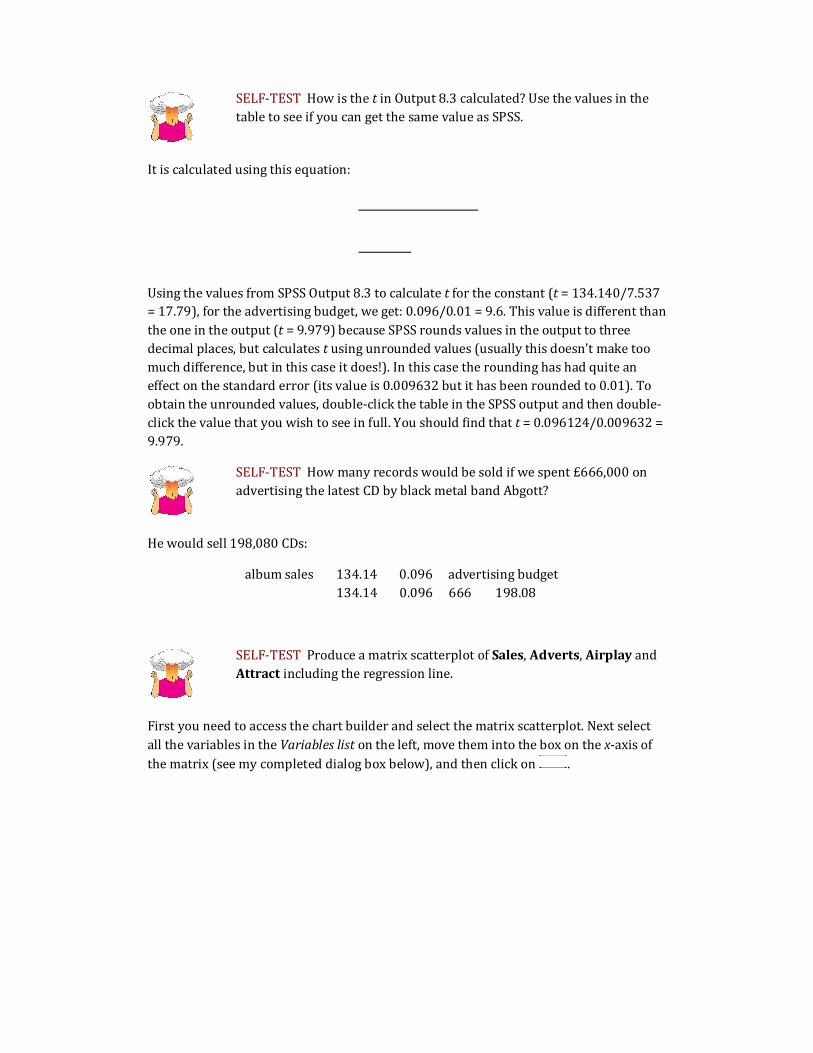
SELF-TEST Produce a matrix scatterplot of Sales, Adverts, Airplay and Attract including the regression line.

First you need to access the chart builder and select the matrix scatterplot. Next select all the variables in the Variables list on the left, move them into the box on the x-axis of the matrix (see my completed dialog box below), and then click on .

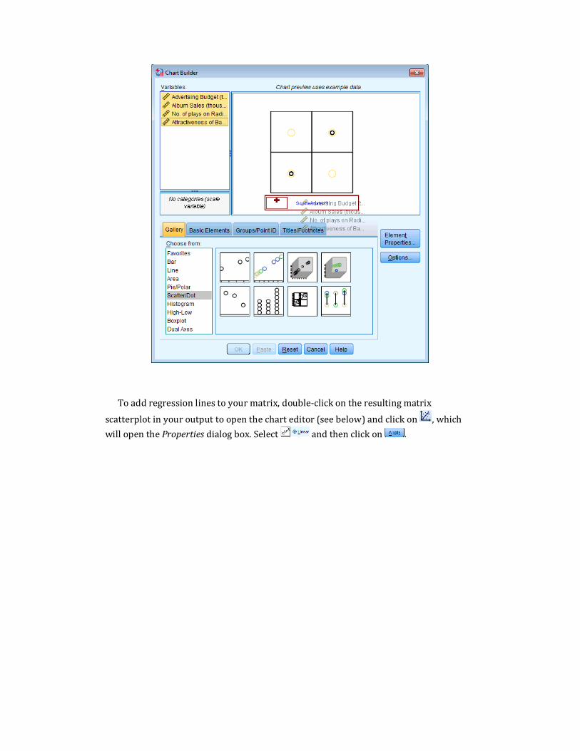
To add regression lines to your matrix, double-click on the resulting matrix

scatterplot in your output to open the chart editor (see below) and click on , which will open the Properties dialog box. Select and then click on .

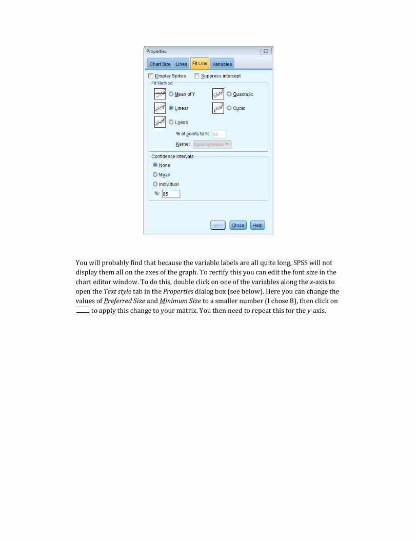
You will probably find that because the variable labels are all quite long, SPSS will not display them all on the axes of the graph. To rectify this you can edit the font size in the chart editor window. To do this, double click on one of the variables along the x-axis to open the Text style tab in the Properties dialog box (see below). Here you can change the values of Preferred Size and Minimum Size to a smaller number (I chose 8), then click on

to apply this change to your matrix. You then need to repeat this for the y-axis.

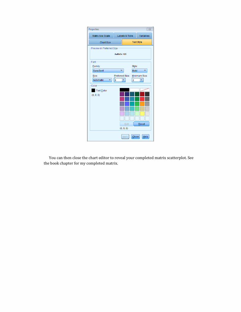
You can then close the chart editor to reveal your completed matrix scatterplot. See the book chapter for my completed matrix.