Simplicial regression. The normal modelfile.statistik.tuwien.ac.at/filz/papers/2011JAPS.pdf · as an alternative model for compositional residuals, but it leads to restrictive and

Simplicial regression. The normal model 1

Simplicial regression. The normal modelJ. J. Egozcue, J. Daunis-i-Estadella, V. Pawlowsky-Glahn, K. Hron and P. Filzmoser

Juan Jose EgozcueDept. Matematica Aplicada III, U. Politecnica de Catalunya (UPC), Barcelona, Spain.

Email: [email protected]

Josep Daunis-i-EstadellaDept. Informatica i Matematica Aplicada, U. de Girona (UdG), Girona, Spain.


Vera Pawlowsky-GlahnDept. Informatica i Matematica Aplicada, U. de Girona (UdG), Girona, Spain.


Karel HronDept. of Mathematical Analysis and Application of Mathematics, Palacky U. (UPOl), Olomouc,

Czech Republic.


Peter FilzmoserDept. of Statistics and Probability Theory, Vienna U. of Technology (TU-Wien, Vienna, Austria.


Abstract

Regression models with compositional response have been studied from the beginningof the log-ratio approach for analysing compositional data. These early approachessuggested the statistical hypothesis of logistic-normality of the compositional residualsto test the model and its coefficients. Also, the Dirichlet distribution has been proposedas an alternative model for compositional residuals, but it leads to restrictive and noteasy-to-use regressions. Recent advances on the Euclidean geometry of the simplexand on the logistic-normal distribution allow re-formulating simplicial regression withlogistic-normal residuals. Estimation of the model is presented as a least-squaresproblem in the simplex and is formulated in terms of orthonormal coordinates. Thisestimation decomposes into simple linear regression models which can be assessedindependently. Marginal normality of the coordinate-residuals suffices to checkinfluence of covariables using standard regression tests. Examples illustrate theproposed procedures.

Keywords: Aitchison geometry, normal distribution on the simplex, isometric log-ratiotransformation (ilr), orthonormal coordinates, log-ratio analysis.

2000 Mathematics Subject Classification: 62J05, 62J02, 86A32, 91B42.

2 J. J. Egozcue et al.

1 Introduction

Compositional data appear frequently in statistical analysis. They quantitatively repre-sent the parts of a whole and only the proportions of their parts are assumed informative.Typical examples are a chemical composition, the proportions of large counts in surveying,the structure of a stock portfolio, the distribution of household expenditures and incomes,etc. As a consequence, compositional data also occur as responses in regression mod-els. Regression models for compositional data were first discussed in [1, 9]. In Aitchisonand Shen [9] a discussion on the distribution of the residuals of the regression is enlight-ening. One obvious candidate was the Dirichlet distribution. The competing model wasthe logistic-normal family of distributions. It was shown that the Dirichlet family can beapproximated by the logistic-normal distribution and thus approximately included in thelogistic-normal family. Moreover, the Dirichlet family seemed to the authors too restrictivefor an effective and practical use in applications [3]. Most of the material about regressionwith compositional responses and the distributions appropriate for residuals presented inthese references keep their validity, and only a little bit about techniques can be added.However, over almost the last three decades these results have not been taken into account,and a lot of studies on Dirichlet regression for compositional responses have appeared.Recent examples are [22, 23, 34].

Recent developments on the simplex geometry [5, 11, 15, 16, 19, 29] allow to expressthe regression model in coordinates and to estimate its coefficients using ordinary leastsquares [12]. When the normal model is assumed for the residuals, its distribution is iden-tified with the logistic-normal or additive-logistic-normal [8, 24]. In this simple case, theleast squares approach can be applied to simplicial coordinates of the compositional re-sponse, and it corresponds to the maximum likelihood estimation of the model. Our objec-tive is to present the linear regression model for compositional response in its coordinateversion. The model can be estimated using ordinary least squares. Under normality of thecoordinate residuals, standard statistical techniques of multiple regression can be applied.As a consequence, the logistic-normal linear regression for compositional responses is thesimplest regression method, competing with other approaches like e.g. models with Dirich-let distributed residuals. Model selection is not treated here globally, but separately for eachcoordinate. Standard techniques in regression analysis can be used on coordinates. Alsomore specific techniques dealing with missing data and rounded zeros have been recentlydeveloped [38].


2 Aitchison simplicial geometry

Geometry

Compositional data of D parts are identified with equivalence classes of proportionalvectors with positive components. A representative of these equivalence classes can betaken to be in the simplex of D parts (equivalently the (D − 1)-dimensional simplex),denoted SD. The simplex SD can be defined as the set of real vectors of D positivecomponents adding to a constant, here assumed to be unity. If x is a D-vector of positivecomponents, denote Cx its representative in the simplex. Cx is readily obtained dividingeach component by their total sum, and is called the closure of x.

A natural operation between elements of the simplex is perturbation, which playsthe role of addition in the simplex. Multiplication by real numbers is called power-ing. Denoting transpose by (·)′, compositions in SD by x = (xα

1 , xα2 , . . . , xα

D)′, y =(y1, y2, . . . , yD)′, and α ∈ R, perturbation and powering are defined as

x⊕ y = C(x1y1, x2y2, . . . , xDyD)′ , α¯ x = C(xα1 , xα

2 , . . . , xαD)′ , (2.1)

respectively. The composition n with equal components is the neutral element for theperturbation. Perturbation and powering (2.1) define a (D − 1)-dimensional vector spacestructure in the simplex SD. The Aitchison inner product in SD is

〈x,y〉a =D∑

i=1

(log xi · log yi)− 1D

D∑

j=1

log xj

·

(D∑

k=1

log yk

). (2.2)

The corresponding norm and distance are

‖x‖a =√〈x,x〉a , da(x,y) = ‖xª y‖a , (2.3)

where ª represents the opposite operation of ⊕, i.e. ªy ≡ ⊕ ((−1)¯ y). The metricsdefined by eq. (2.2), resp. (2.3), is compatible with the operations in (2.1), so that thesimplex

(SD,⊕,¯, 〈., .〉a)

is a (D − 1)-dimensional Euclidean space [5, 11, 29]. Thisconstitutes the so-called Aitchison geometry of the simplex.

A consequence of the Euclidean structure of SD is that an orthonormal basis of thespace can be built, and a composition x ∈ SD can be represented by its coordinates withrespect to such a basis. Let x∗ = h(x) be the vector of D − 1 real coordinates of x. Foreach orthonormal basis, the coordinate function h(·) is an isometry between SD andRD−1,called isometric log-ratio transformation [19]. Important properties of such an isometry are

h(x⊕ y) = h(x) + h(y) , h(α¯ x) = α · h(x) , (2.4)

and

〈x,y〉a = 〈h(x), h(y)〉 , ‖x‖a = ‖h(x)‖ , da(x,y) = d(h(x), h(y)) , (2.5)


where 〈·, ·〉, ‖ · ‖ and d(·, ·) are the ordinary Euclidean inner product, norm and distancein RD−1 respectively. This means that, whenever compositions are transformed into coor-dinates, the metrics and operations in the Aitchison geometry of the simplex are translatedinto the ordinary Euclidean metrics and operations in real space.

The choice of an orthonormal basis can be made following the methods developedin [16,17]. They consist of defining a sequential binary partition (SBP) of the compositionalvector. In a first step, the components of the composition are divided into two groups;components in one group are marked with a +1 and components in the other group aremarked with a −1; see Table 2.1, order 1 row. In a second and following steps, a previousgroup of parts is divided into two new groups and they are similarly marked with +1 and−1, while the components not involved are marked with 0; see second and following rowsin Table 2.1. The number of steps required until each group contains a single component

Table 2.1: Coding of a sequential binary partition (SBP) of a D = 5 compositional vector x. Eachrow of the (4, 5)-matrix Θ indicates with +1 and−1 the components in each group of the partition atthe corresponding order; 0 indicates that the component does not participate in the partition. Columnsr, resp. s, are the number of +1, resp. −1, in the corresponding order partition. The balance-coordinate is made explicit in the last column.

order x1 x2 x3 x4 x5 r s balance

1 +1 −1 −1 +1 +1 3 2 x∗1 = (6/5)1/2 log (x1x4x5)1/3

(x2x3)1/2

2 +1 0 0 +1 −1 2 1 x∗2 = (2/3)1/2 log (x1x4)1/2

x5

3 +1 0 0 −1 0 1 1 x∗3 = (1/2)1/2 log x1x4

4 0 −1 +1 0 0 1 1 x∗4 = (1/2)1/2 log x3x2

is exactly D − 1, i.e. the dimension of SD. Let Θ = [θij ] be a (D − 1) × D matrixcontaining the codes represented in Table 2.1. An element of an orthonormal basis of SD,and the corresponding coordinate, are associated with each row of Θ. First, for the ith-rowof Θ compute the number of +1 and −1 and denote them by ri and si, respectively. Then,construct the (D − 1)×D matrix Ψ = [ψij ] where

ψij = θijs(θij−1)/2i

r(θij+1)/2i

√risi

ri + si, i = 1, 2, . . . , D − 1 , j = 1, 2, . . . , D . (2.6)

The matrix Ψ (2.6) has some remarkable properties, similar to those of Helmert matrices[37]. The coordinate associated with the i-th row of Θ is

x∗i =√

risi

ri + silog

∏+ x

1/ri

j∏− x

1/si

k

, (2.7)


where the product subscripted + (resp. −) runs over the components marked with +1 (resp.−1) in the i-th row of Θ. The transformation into coordinates (2.7) is called isometric log-ratio transformation (ilr) [16,19]. The coordinates are also called balances because of theirparticular form as ratios of geometric means of components grouped as coded in the SBP,as shown in (2.7). The computation of the balances or coordinates of the composition canbe written as

x∗ = h(x) = Ψ · log x , (2.8)

where the logarithmic function applies componentwise and the dot denotes matrix product.A composition can be readily recovered from its coordinates using the inverse ilr transfor-mation

x = h−1(x∗) = C exp(Ψ′ · x∗) , (2.9)

where exp(.) applies componentwise to the argument vector [37].There are other ways of representing elements of the simplex. Two of them, called

alr and clr [3], additive log-ratio and centered log-ratio transformations respectively, arehistorically previous to orthogonal coordinates, ilr, and have been used extensively. Thealr transformation of a composition x ∈ SD is defined as the (D − 1)-real vector

alr(x) = log(

x1

xD,

x2

xD, . . . ,

xD−1

xD

)′, (2.10)

with inverse transformation

alr−1(y) = C exp (y1, y2, . . . , yD−1, 0)′ , (2.11)

where y = alr(x) ∈ RD−1. The components of alr(x) are coordinates of the compositionwith respect to an oblique basis of the simplex [16]. This means that it can be useful forrepresentations where the properties of SD as a vector space play the main role. However,the alr representation may be not easy to use when dealing with metric properties of SD.

For x ∈ SD, the centered log-ratio transformation clr is defined as

clr(x) = log(

x1

g(x),

x2

g(x), . . . ,

xD

g(x)

)′, (2.12)

where g(·) is the geometric mean of the components of the argument. The clr representationis an isometry between SD with the Aitchison geometry and the (D − 1)-dimensionalsubspace of RD of vectors whose components add to zero. Therefore, components of theclr transformed vectors add to zero, thus constraining its components. The clr components(2.12) permit the reconstruction of the corresponding composition

x = C exp(y) , (2.13)

where y = clr(x) ∈ RD. The clr representation of compositions is very useful to computeoperations and metrics in SD, although a redundant component is used in the storage and


in computation. Examples of use of the clr (2.12), (2.13) are the computation of composi-tional principal components [2, 3] and compositional biplots [6].

Elements of simplicial statistics

When dealing with random compositions, i.e. random vectors whose sample spaceis SD, the Aitchison simplicial geometry influences some elementary concepts, speciallythose related with the underlying metrics of the sample space. The mean and variance, andthe respective estimators, are here addressed. Also the normal distribution in the simplexand its representation is briefly presented.

The concept of centre of a random composition, X, was introduced in [4]. It can bedefined as

Cen[X] = h−1E[h(X)] = C exp(E[log X]) , (2.14)

where h(·) is the coordinate function for a chosen basis in SD and E[·] is the ordinaryexpectation in the real space RD. The second member in (2.14) corresponds to a DeFinettigamma-mean [13]. The third member in (2.14) is the expression given by Aitchison,which is proportional to a geometric mean. Note that the definition does not depend onthe chosen basis in SD. The center can also be defined as the element in SD minimizingthe Aitchison-metric variability of X, which does not depend on the basis [29]. In a moregeneral framework, this definition is in agreement with the general theory developed in[14]. Given a random sample of X, the natural estimator of Cen[X] is the simplex-averageor geometric mean [30]

X =1n¯

n⊕

i=1

xi = C

(n∏

i=1

xi1

)1/n

,

(n∏

i=1

xi2

)1/n

, . . . ,

(n∏

i=1

xiD

)1/n′

, (2.15)

where xi = (xi1, xi2, . . . , xiD)′ is the ith-sample composition. This estimator is unbiasedin the simplex, i.e. Cen[Xª Cen[X]] = n.

The metric or total variance of a random composition [4,29] is defined in a natural wayas

MVar[X] = E[d2a(X, Cen[X])] . (2.16)

There are a number of expressions of (2.16) in terms of log-ratios of the components of therandom composition. When using coordinates X∗ of the random composition with respectto a chosen basis, MVar[X] is decomposed into variances of the coordinates [18], i.e.

MVar[X] =D−1∑

j=1

Var[X∗j ] , (2.17)

where X∗j denotes de jth-coordinate of the random composition X. The decomposition

(2.17) holds after the decomposition of the Aitchison-distance using orthonormal coordi-


nates [16]. The estimation is then reduced to the estimation of the variances of the coor-dinates Var[X∗

j ]. The CoDa-dendrogram can be used for a visualization of the variancedecomposition [18, 31, 35]. The covariances between coordinates complete the second or-der description of the variability of the random composition. They can be arranged in thevariance-covariance (D− 1, D− 1)-matrix Σ whose ij-entry is Cov[X∗

i , X∗j ]. The matrix

Σ depends on the selected basis. However, the covariance endomorphism represented byΣ is invariant under changes of basis in SD [14, 36].

3 Least squares regression with a compositional response.

Consider a n-sample data set in which the i-th record is made of a compositional re-sponse xi = (xi1, xi2, . . . , xiD)′ in SD, and the values of r covariates arranged in a vectorti = (t0, ti1, ti2, . . . , tir)′, where t0 = 1 is equal for each record. A prediction in thesimplex SD consists of a deterministic function of the covariates, also called predictor,p(t) ∈ SD; and a perturbation-additive error or residual e ∈ SD. A linear predictor in thesimplex is

p(t) =r⊕

k=0

(tk ¯ bk) , (3.1)

where the coefficients bk ∈ SD. The predictor (3.1), is a linear combination of compo-sitional coefficients bk, with respect to the Aitchison geometry of the simplex, where thecoefficients of the combination are the real covariates. The covariate t0 = 1 provides aconstant term in the predictor.

The least squares regression problem is to find estimates, bk, of the compositionalcoefficients bk, k = 0, 1, . . . , r, in

xi = b0 ⊕r⊕

k=1

(tik ¯ bk)⊕ ei , i = 1, 2, . . . , n , (3.2)

minimizing the sum of square-norms of the error

SSE =n∑

i=1

‖ei‖2a =n∑

i=1

‖p(ti)ª xi‖2a . (3.3)

The regression model (3.2) contains (r +1)×D parameter values to be determined. How-ever, the bk’s are in the simplex and D − 1 components determine these coefficients and,therefore, there are only (r + 1) × (D − 1) parameters to be estimated from the data. Itis worth to remark that all familiar geometrical concepts in (3.2) and (3.3), like linearity,deviation, norm, are here referred to the Aitchison geometry of the simplex. Accordingly,SSE (3.3) cannot be compared to similar expressions in which the norms and operationsare those of the standard real Euclidean space. The adequacy of SSE as a target function


to be minimized relays on the compositional character of the response and the consequentmeasurement of deviations in SD.

Assume that the least-squares estimate of the compositional coefficients are bk, thusdefining the predictor p(t). The corresponding estimated residuals are ei and SSE denotesthe minimized sum of squares. Similarly to the standard multiple linear regression analysis,the total sum of squares SST, defined as

SST =n∑

i=1

‖xi ªX‖2a , (3.4)

is considered. The statistics X in (3.4) is the geometric average of the sample responseas defined in (2.15). The statistics n−1 · SST is an estimator of the total variance of theresponses MVar[X] (2.16). Also, a sum of squares explained by the regression model canbe defined as

SSR =n∑

i=1

‖p(ti)ªX‖2a , (3.5)

which gives rise to a decomposition of SST:

SST = SSR + SSE . (3.6)

The reasoning to arrive to the decomposition (3.6) is parallel to that of the ordinary real mul-tivariate linear regression. Similarly, a determination coefficient of the regression modelcan be defined as

R2 =SSR

SST= 1− SSE

SST, (3.7)

which is interpreted as the per unit of metric-variance of the compositional response ex-plained by the regression.

The least-squares problem can be efficiently solved expressing the compositional re-sponses in coordinates, specifically with respect to an orthonormal basis of the simplex.If h(·) is the coordinate function for the chosen orthonormal basis, denote x∗i = h(xi),e∗i = h(ei) for i = 1, 2, . . . , n; and b∗k = h(bk), k = 0, 1, . . . , r. Taking coordinates in(3.2), the transformed model is

x∗i = b∗0 +r∑

k=1

(tik · b∗k) + e∗i , i = 1, 2, . . . , n , (3.8)

and, using (2.17),

SSE =n∑

i=1

‖e∗i ‖2 =n∑

i=1

D−1∑

j=1

(e∗ij)2 . (3.9)

Eq. (3.9) is a consequence of the isometric character of h(·): the Aitchison norm of acomposition is equal to the ordinary real Euclidean norm of its coordinates (2.5). In the


expression of SSE (3.9), the order of the sums can be inverted and, being all terms non-negative, the minimization of SSE in coordinates is equivalent to the separate minimizationof the D − 1 terms

SSEj =n∑

i=1

(e∗ij)2 =

n∑

i=1

(xij −

r∑

k=0

tkb∗kj

)2

, j = 1, 2, . . . , D − 1 , (3.10)

where b∗kj is the j-th coordinate of the compositional coefficient bk. Comparing (3.9) and(3.10), the Pythagorean decomposition

∑D−1j=1 SSEj = SSE is easily obtained. For the j-th

coordinate, (3.10) implies the ordinary least-squares solution of the real regression model

x∗ij =r∑

k=0

tkb∗kj + e∗ij , i = 1, 2, . . . , n , (3.11)

where e∗ij is the j-th coordinate of the compositional residual ei. Eqs. (3.10) and (3.11)imply that the least-squares regression problem in the simplex (3.2), (3.3) is equivalent toD − 1 ordinary least-squares problems for the coordinates (3.10) and (3.11). Remarkably,the least-squares problems for the coordinates can be solved independently. Moreover, theresults are independent of the selected orthonormal basis: although the coordinates of theobtained coefficients bk and residuals ei depend on the selected basis, the reconstructedcompositional coefficients and residuals using (2.9) do not.

For each regression problem (3.11), (3.10), the sum of squares decomposition holds,i.e. SSE =

∑D−1j=1 SSEj and SSR =

∑D−1j=1 SSRj . The determination coefficient can also

be expressed in terms of the sums of squares of the regression for the coordinates,

R2 =

∑D−1j=1 SSRj

SST=

∑D−1j=1 SSTj ·R2

j

SST, (3.12)

where R2j = SSRj/SSTj is the determination coefficient for the regression of the jth-

coordinate of the response.The whole procedure may be summarized in the following steps: (i) select an orthonor-

mal basis, possibly using a sequential binary partition (SBP) of the compositional responsevector; (ii) represent the compositional response by means of its orthonormal coordinates,possibly balance-coordinates; (iii) perform the least-squares estimation of the regressioncoefficients and the sums of squares for each coordinate of the response using the avail-able covariates; (iv) reconstruct, if necessary, the compositional coefficients, predictor andresiduals. These steps correspond to the principle of working on coordinates [27].

The standard practice in logistic regression [1, 7, 28] , in spatial cokriging [32] or evenin simplicial regression [11, 12], has not been to use the ilr transformation (orthonormalbasis representation) but the alr transformation (oblique basis representation). A naturalquestion is which is the difference in the least-squares results when using these two dif-ferent representations of the compositional response. In fact, there is no difference in the


estimated compositional coefficients of the regression model (3.2) and, consequently, thecompositional residuals are also equal. The difference appears when trying to obtain thedecomposition of SST (3.6) into the alr-coordinate contributions (3.4). When using alr-coordinates,

∑D−1j=1 SSTj ≥ SST,

∑D−1j=1 SSRj 6= SSR, and

∑D−1j=1 SSEj 6= SSE. In

order to compute the sums of squares it is then necessary to obtain the compositional pre-dictors and residuals and to compute SSR and SSE using their definition (3.5),(3.3) and theAitchison-norm (2.3). It is remarkable that in standard multinomial logistic regression thereare difficulties for defining a determination coefficient. This is related to the representationof the response probabilities using alr-coordinates.

4 The normal model of compositional residuals

4.1 Normal distribution on the simplex

A statistical analysis of a regression model requires further hypotheses on the distri-bution of the residuals. The simplest model with compositional residuals is that of thelogistic-normal distribution introduced by Aitchison and Shen [9], also to be found in [1,3].There, the logistic-normal model is compared with the Dirichlet distribution approach forthe residuals. The main argument against the Dirichlet approach is that this distributionis too restrictive and imposes strong conditions on the dependence between components.Moreover, the Dirichlet distribution can be suitably approximated (in the sense of Kullback-Leibler divergence) by some distributions in the logistic-normal family. This gives sense tothe point put forward by Aitchison and Shen [9], which remains still open: Can we developsatisfactory tests of the separate families, Dirichlet and logistic-normal, along the linesof Cox (1962)? In particular, to what extent are current tests of multivariate normalitypowerful against the Dirichlet alternative?

The main argument in favour of the logistic-normal distribution is the invariance of thefamily under perturbations in the simplex. An important consequence is the central limittheorem for the logistic-normal distribution, sketched in Aitchison [3]. This makes thelogistic-normal distribution a natural one.

The logistic-normal distribution can be defined in different ways. The original def-initions by J. Aitchison are based on the normality of the alr coordinates of a randomcomposition. More recently, and following the lines proposed by Eaton [14], an intrinsicdefinition independent of coordinates is available [36]. Here the definition is based on therepresentation in orthonormal coordinates [24–26].

Consider a random composition X ∈ SD whose representation in coordinates withrespect to a selected orthonormal basis is X∗ ∈ RD−1, X∗ = h(X). The random com-position X has a logistic-normal distribution or, equivalently, a normal distribution in thesimplex, whenever X∗ has a multivariate normal distribution, i.e. X∗ ∼ N (µ∗,Σ∗). Then


X ∼ NSD (µ∗,Σ∗), with Cen[X] = h−1(µ∗).When the normal in the simplex is represented by a probability density, it is better

to take the Aitchison measure than the Lebesgue measure as reference. The probabilitydensity of X ∼ NSD (µ∗, Σ∗) with respect to the Aitchison measure is

fSX(x) = (2π)−(D−1)/2 |Σ∗|−1/2 exp(−1

2(x∗ − µ∗)′Σ∗−1(x∗ − µ∗)

), (4.1)

where x is an element of the simplex SD and x∗ is the vector of coordinates with respectto a given orthonormal basis. Note the absence of a Jacobian in (4.1); it is cancelled whenchanging the reference measure [24]. The density (4.1) is actually the Radon-Nikodymderivative of the probability with respect to the Aitchison measure in the simplex.

If the Lebesgue measure is used as reference, the logistic-normal density has the ex-pression

fX(x) =(2π)−(D−1)/2 | Σ∗ |−1/2

√D x1x2 · · ·xD

exp(−1

2(x∗ − µ∗)′Σ∗−1(x∗ − µ∗)

), (4.2)

where the denominator is the Jacobian of the coordinate transformation [24].

Normal compositional residuals

The standard statistical model for linear regression assumes that the residuals are in-dependent and normally distributed. Similarly, independence and normality in the simplexare here assumed for the compositional residuals in the regression model (3.2). This as-sumption permits to use likelihood ratio tests to check global hypotheses on the regressionmodels. They were developed in [3] and then used in a lattice of hypothesis with increasingcomplexity, to arrive to an appropriate regression. No further development is here offeredin these aspects. However, expressing the regression model in orthonormal coordinates,conveys an additional result, not clearly developed previously: the standard battery of test-ing hypotheses for linear regression models can be applied to the regression model for eachorthogonal coordinate (3.11). Therefore, marginal normality of each coordinate residual isenough to use regression tests based on normality. However, these marginal tests dependin general on the selected basis of the simplex.

5 Illustrative examples

In the following examples, we apply the above mentioned theoretical considerationsto real data cases from different fields of interest, namely economics and geochemistry.Special attention will be devoted to the construction of balances and to the interpretationof results.


Example 1 (Household expenditures) The first data set comes from Eurostat (Euro-pean Union statistical information service) and represents mean consumption expendi-tures of households on 12 domestic year costs in all 27 Member States of the Euro-pean Union (EU) in 2005; it is available at http://epp.eurostat.ec.europa.eu/statistics explained/index.php/Household consumption expenditure. Thedata are displayed in Table 5.2, together with the gross domestic product (GDP) for 2009,one of the well known measures of a country’s overall economic performance that was ob-tained from public sources of the internet encyclopedia Wikipedia. The GDP represents themarket value of all final goods and services made within the borders of a country in a year.In order to offer a better insight into the construction and interpretation of balances, wefocus on a subcomposition of four parts, that include expenditures on foodstuff, housing(including water, electricity, gas and other fuel), health, and communications. The first twoparts thus represent basic costs, while the latter two rather ”external” costs that seem to bemore or less related to economic status and, consequently, also to quality of life in eachmember state. However, to see the influence of GDP, not the absolute values as in Table5.2, but the ratios between the expenditures are of interest. Since the absolute values areinfluenced by the overall price levels in the single states, their direct analysis would leadto meaningless results. The closed geometric mean of the chosen expenditures (denotedx1, . . . , x4) is X = (0.364, 0.496, 0.066, 0.074)′, i.e. the expenditures on housing clearlydominate.

Table 5.2 shows that the GDP of Luxembourg is considerably higher than for the othercountries. Since the least squares method is very sensitive to outlying observations, espe-cially in the direction of an explanatory variable, this could essentially change the resultsof regression analysis and affect the final interpretation. For this reason, we exclude Lux-embourg from further computations.

To see the effect of the GDP on both basic and external costs using regression anal-ysis, we decompose the relative information contained in the (sub)composition, into bal-ances. Here it seems natural to separate the parts x1 and x2, representing the basic costs,from the external ones, x3 and x4. The corresponding SBP is displayed in Table 5.3.Thus, the first coordinate, x∗1, represents the balance between the parts x1, x2 and the partsx3, x4, or equivalently expressed, it explains the four ratios between foodstuff and hous-ing on one side, and health and communications on the other side. The second balance,x∗2, then explains the ratio between foodstuff and housing, and x∗3 the remaining ratio be-tween health and communications. The variances of the balances are Var[X∗

1 ] = 0.060,Var[X∗

2 ] = 0.166 and Var[X∗3 ] = 0.144. Taking into account Eq. (2.17) for the metric

variance, MVar[X], one can conclude that the second and third balance explain most of thevariability contained in the composition.

For all three balances we apply the regression model according to (3.11). The obtainedregression lines are displayed in Figure 5.1. Since in the following we assume normal


Table 5.2: GDP per capita (2009) and mean consumption expenditures of households on 12 domesticyear costs (2005; both in Euro) in all 27 Member States of the European Union.

Mem

berS

tate

GDP

foodstuff

housing

alcohol and tobacco

clothing and footwear

household equipment

health

transport

communications

recreation and culture

education

restaurants and hotels

miscellaneous

Aus

tria

2970

039

3367

3284

716

8218

6894

648

6379

338

0924

216

6027

92B

elgi

um28

100

4043

7610

669

1425

1687

1400

3863

878

2868

136

1894

3576

Bul

gari

a92

0022

3824

6126

921

821

330

535

532

520

434

255

220

Cyp

rus

2250

051

5873

8164

626

4920

0816

2449

8011

6420

4413

5428

3023

70C

zech

Rep

ublic

1890

025

0324

4434

767

981

523

913

5155

512

8966

619

1234

Den

mar

k27

600

2872

7194

785

1168

1459

639

3331

583

2738

100

960

2233

Est

onia

1430

024

4032

4030

060

156

828

210

8759

669

114

533

955

9Fi

nlan

d26

600

3086

6614

588

934

1238

852

3818

693

2731

5110

2127

33Fr

ance

2600

037

3373

3965

018

5316

9311

6737

7791

419

2616

512

7733

92G

erm

any

2730

031

8584

4548

913

5515

4310

2437

9082

831

6823

612

1232

26G

reec

e23

200

4801

7442

1045

2154

1929

1824

3222

1174

1285

738

2661

2701

Hun

gary

1480

024

1320

7338

053

749

844

015

1169

690

990

343

803

Irel

and

3220

044

9185

2020

3218

5126

1390

442

0312

5536

7068

721

9039

56It

aly

2330

053

5985

1250

620

1316

7011

3234

2062

116

8020

214

2822

42L

atvi

a11

300

3091

1810

329

778

546

394

1155

610

667

145

557

508

Lith

uani

a12

500

3166

1776

332

743

392

445

762

435

402

102

429

393

Lux

embo

urg

6330

048

5115

611

865

3343

3702

1351

8403

1139

3869

223

4098

4478

Mal

ta18

800

6082

2596

786

2387

3070

869

4758

837

2879

352

2030

1960

Net

herl

ands

3120

030

8975

1362

516

9418

8837

131

9690

331

9330

616

4749

45Po

land

1410

027

0433

4126

248

947

848

586

251

266

213

818

057

1Po

rtug

al18

100

3243

5560

477

861

994

1264

2693

616

1182

356

2263

1359

Rom

ania

1020

023

5583

230

733

320

120

534

425

922

445

5816

2Sl

ovak

ia16

500

2910

2517

333

661

494

330

986

506

712

9252

071

3Sl

oven

ia21

200

3966

5483

575

1678

1389

356

3717

950

2234

202

1035

2220

Spai

n24

500

4685

7874

586

1786

1211

577

2743

701

1659

292

2414

1499

Swed

en28

300

2913

8250

531

1270

1640

638

3623

791

3398

898

115

69U

nite

dK

ingd

om27

600

3159

9458

753

1585

2092

383

4305

852

3943

457

2558

2415

Abb

revi

atio

nt

x1

x2

--

-x3

-x4

--

--


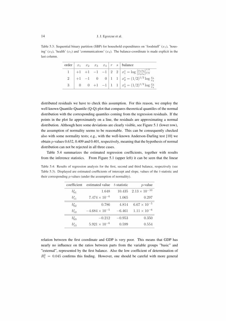
Table 5.3: Sequential binary partition (SBP) for household expenditures on ’foodstuff’ (x1), ’hous-ing’ (x2), ’health’ (x3) and ’communications’ (x4). The balance-coordinate is made explicit in thelast column.

order x1 x2 x3 x4 r s balance

1 +1 +1 −1 −1 2 2 x∗1 = log (x1x2)1/2

(x3x4)1/2

2 +1 −1 0 0 1 1 x∗2 = (1/2)1/2 log x1x2

3 0 0 +1 −1 1 1 x∗3 = (1/2)1/2 log x3x4

distributed residuals we have to check this assumption. For this reason, we employ thewell known Quantile-Quantile (Q-Q) plot that compares theoretical quantiles of the normaldistribution with the corresponding quantiles coming from the regression residuals. If thepoints in the plot lie approximately on a line, the residuals are approximating a normaldistribution. Although here some deviations are clearly visible, see Figure 5.1 (lower row),the assumption of normality seems to be reasonable. This can be consequently checkedalso with some normality tests; e.g., with the well-known Anderson-Darling test [10] weobtain p-values 0.632, 0.409 and 0.401, respectively, meaning that the hypothesis of normaldistribution can not be rejected in all three cases.

Table 5.4 summarizes the estimated regression coefficients, together with resultsfrom the inference statistics. From Figure 5.1 (upper left) it can be seen that the linear

Table 5.4: Results of regression analysis for the first, second and third balance, respectively (seeTable 5.3). Displayed are estimated coefficients of intercept and slope, values of the t-statistic andtheir corresponding p-values (under the assumption of normality).

coefficient estimated value t-statistic p-value

b∗01 1.648 10.435 2.13× 10−10

b∗11 7.474× 10−6 1.065 0.297

b∗02 0.786 4.814 6.67× 10−5

b∗12 −4.684× 10−5 −6.461 1.11× 10−6

b∗03 −0.212 −0.953 0.350

b∗13 5.921× 10−6 0.599 0.554

relation between the first coordinate and GDP is very poor. This means that GDP hasnearly no influence on the ratios between parts from the variable groups ”basic” and”external”, represented by the first balance. Also the low coefficient of determination ofR2

1 = 0.045 confirms this finding. However, one should be careful with more general


10000 15000 20000 25000 30000

1.4

1.6

1.8

2.0

2.2

GDP

x1*

10000 15000 20000 25000 30000

−0.5

0.0

0.5

GDPx2*

10000 15000 20000 25000 30000

−0.6

−0.4

−0.2

0.0

0.2

0.4

GDP

x3*

−2 −1 0 1 2

−0.4

−0.2

0.0

0.2

0.4

Normal Q−Q Plot

Theoretical Quantiles

Sam

ple

Quantile

s

−2 −1 0 1 2

−0.4

−0.2

0.0

0.2

0.4

0.6

Normal Q−Q Plot


Sam

ple

Quantile

s

−2 −1 0 1 2

−0.6

−0.4

−0.2

0.0

0.2

0.4

0.6

Normal Q−Q Plot

Theoretical QuantilesS

am

ple

Quantile

s

Figure 5.1: Regression for the first (upper left), second (upper middle) and third (upper right) balancein dependence on GDP, together with the resulting regression lines. In the lower row Q-Q plots forresiduals of the corresponding regression models are displayed.

conclusions, because by construction of the first balance, a nearly constant relation ofthe balance to GDP can also be reached by an increase of one ratio and a decreaseof the other ratio by about the same amount. For the second balance, that describesonly the ratio foodstuff/housing, a decreasing trend is clearly visible, confirmed by thecorresponding t-statistic (see Table 5.4) as well as by R2

2 = 0.635. From the constructionof the coordinate x∗2 (see Table 5.3), this corresponds to a decreasing ratio betweenfoodstuff and household expenditures for increasing values of GDP. This is somewhatin contradiction with our intuition, since we would expect a rather constant relationbetween GDP and the ratio of the basic costs. Finally, the regression of the third balanceon GDP shows that the ratio between the selected external costs is independent fromthe economic status of the member states; here R2

3 = 0.015. Again, one would ratherexpect a systematic influence of the GDP. Using (3.12) we obtain the coefficient ofdetermination for the whole regression model, R2 = 0.323. Note that another choice ofSBP would enable to focus also on the other ratios induced by the investigated composition.

Example 2 (Concentrations of chemical elements) Here we employ the well-known Koladata set which resulted from a large geochemical mapping project, carried out from 1992 to


1998 by the Geological Surveys of Finland and Norway, and the Central Kola Expedition,Russia. An area covering 188000 km2 in the Kola peninsula of Northern Europe was sam-pled (Figure 5.2). In total, approximately 600 samples of soil were taken in four different

0

5

25

50

75

90

95

100

15.0

59.0

140

200

260

320

360

540

Percentile MetersElevation

0 50 100 km

N

Figure 5.2: Map of the Kola peninsula, lighter shadings correspond to higher altitude.

layers (moss, O-horizon, B-horizon, C-horizon) and subsequently analyzed by a numberof different techniques for more than 50 chemical elements. The project was primarily de-signed to reveal the environmental conditions in the area; more details can be found in [33].The whole data set is available in package StatDA [21] of the statistical software R. Forour study, three chemical elements from the O-horizon were taken, Fe (iron, x1), K (potas-sium, x2), and P (phosphorus, x3), and their values are reported in mg/kg. The elementconcentrations are depending on different geological processes, but also other effects playan important role, like the climatic zones (corresponding to the latitude) or the elevation(Figure 5.2). Especially elements like potassium (K) and phosphor (P) are likely to dependon latitude and/or elevation, because they both form a nutrient base for plants. However,from the maps of the single element concentrations [33] it is not easy to detect whetherelevation is indeed a dominant effect for the element concentrations. With three-part com-positions, we have the possibility to visualize the observations in a ternary diagram (Figure5.3, left). Here, the symbol size is proportional to the elevation. However, any systematicpattern is not visible (analogously also longitude and latitude as location variables wouldshow no clear effects).

The distribution of the concentrations of Fe, and in particular of K and P in the studyarea can be revealed by employing the same strategy for the sequential binary partition as


Fe K

P

0 1 2 3

−1.0

−0.5

0.0

0.5

1.0

z1

z2

Figure 5.3: Ternary diagram (left) and coordinate representation (right) of the elements Fe, K, P fromO-horizon of the Kola data.

in the previous example. Thus, in the first balance we separate Fe from the other elementsand the second balance of interest will correspond to the logratio between both nutrientbase elements K and P. The sequential binary partition is displayed in Table 5.5 and theresulting coordinates are shown in Figure 5.3 (right). Here some departures from the maindata cloud are clearly visible, and they are due to outliers in the ratio K and P, expressedby the second balance. One of the main questions is whether the concentrations of the

Table 5.5: Coding a sequential binary partition (SBP) for the composition Fe, K, P of the O-horizonin Kola data. The balance-coordinate is made explicit in the last column.

order x1 x2 x3 r s balance

1 +1 −1 −1 1 2 x∗1 = (2/3)1/2 log x1(x2x3)1/2

2 0 −1 +1 1 1 x∗2 = (1/2)1/2 log x3x2

elements are uniformly distributed in the study area, and whether an influence of elevationcan be demonstrated. For this purpose, we construct regression models for both balances,with longitude, latitude and elevation as explanatory variables. The results are summa-rized in Table 5.6. The first balance, that explains the ratios Fe/K and Fe/P, confirms ourpreliminary expectations. Elevation is significant in the regression model, and longitudeis nearly significant on the usual significance level α = 0.05. Since Fe is supposed to beindependent from location and elevation, the parts K and/or P will be responsible for thesignificance. Also for the ratio P to K, expressed by the second balance, both elevation and


Table 5.6: Results of regression analysis for the first and second balance, respectively. Displayed areestimated coefficients of intercept and slope, values of the t-statistic and their corresponding p-values(under the assumption of normality).

parameter coefficient estimated value t-statistic p-value

intercept b∗01 2.431 1.616 0.107

longitude b∗11 3.290× 10−7 1.752 0.080

latitude b∗21 −2.717× 10−7 −1.424 0.155

elevation b∗31 5.502× 10−4 2.144 0.032

intercept b∗02 0.374 0.621 0.5350

longitude b∗12 −1.358× 10−7 −1.806 0.0715

latitude b∗22 −5.685× 10−8 −0.744 0.4570

elevation b∗32 6.035× 10−4 5.875 6.92× 10−9

longitude play an important role in the regression model. The elevation is highly signifi-cant, with a p-value of 6.92× 10−9, revealing that the construction of the balances for theregression model was able to confirm our expectations that plant nutrients indeed dependon the altitude. In fact, the ratio of P to K is increasing with increasing elevation.

The Q-Q plots of the residuals for both balances are presented in Figure 5.4 (upperrow). They show certain deviations from normality, and thus care has to be taken with thevalidity of the results. A possible solution could be to use robust methods that are able todeal with certain deviations from normality [20]. On the other hand, the above findings canbe compared with maps of the values of both balances, see Figure 5.4, lower row. Indeed,the effect of elevation on the first balance is visible in the map (lower left), and even moreclearly visible for the second balance (lower right).

6 Conclusion

Regression models with compositional response were proposed in the eighties. Thenatural statistical hypothesis was that compositional residuals follow logistic-normal dis-tribution. Using the Euclidean structure of the simplex, the response variables can be rep-resented using orthogonal coordinates. The estimation of model coefficients is formulatedas a least-squares problem with respect to the Aitchison geometry of the simplex and thentranslated into coordinates. Each coordinate can be studied separately under marginal nor-mality of coordinate residuals using a standard and simple regression model. Formulated inthis way, simplicial regression under logistic-normal residuals is a natural and easy-to-usemodel.


−3 −2 −1 0 1 2 3

−1

01

2

Normal Q−Q Plot for first balance


Sam

ple

Quantile

s

−3 −2 −1 0 1 2 3

−1.0

−0.5

0.0

0.5

1.0

Normal Q−Q Plot for second balance


Sam

ple

Quantile

s

05

2550759095

100

−0.66−0.11

0.280.651.011.391.643.20

PercentileFirst balance

0 50 100 km

N

05

2550759095

100

−1.26−0.30−0.13−0.04

0.090.230.331.27

PercentileSecond balance

0 50 100 km

N

Figure 5.4: Q-Q plots of the residuals resulting from regressions with the first and second balance,respectively (upper row), and maps of the balances (lower row).


References

[1] Aitchison, J., 1982: The statistical analysis of compositional data (with discussion).Journal of the Royal Statistical Society, Series B (Statistical Methodology), 44(2),139–177.

[2] Aitchison, J., 1983: Principal component analysis of compositional data. Biometrika,70(1), 57–65.

[3] Aitchison, J., 1986: The Statistical Analysis of Compositional Data. Monographs onStatistics and Applied Probability. Chapman & Hall Ltd., London (UK). (Reprintedin 2003 with additional material by The Blackburn Press). 416 p.

[4] Aitchison, J., 1997: The one-hour course in compositional data analysis or composi-tional data analysis is simple. In Proceedings of IAMG’97 — The third annual confer-ence of the International Association for Mathematical Geology, Pawlowsky-Glahn,V., editor, volume I, II and addendum, International Center for Numerical Methods inEngineering (CIMNE), Barcelona (E), 1100 p, 3–35.

[5] Aitchison, J., C. Barcelo-Vidal, J. J. Egozcue, and V. Pawlowsky-Glahn, 2002: Aconcise guide for the algebraic-geometric structure of the simplex, the sample spacefor compositional data analysis. In Proceedings of IAMG’02 — The eigth annualconference of the International Association for Mathematical Geology, Bayer, U.,Burger, H., and Skala, W., editors, volume I and II, International Association forMathematical Geology, Selbstverlag der Alfred-Wegener-Stiftung, Berlin, 387–392.

[6] Aitchison, J. and M. Greenacre, 2002: Biplots for compositional data. Journal of theRoyal Statistical Society, Series C (Applied Statistics), 51(4), 375–392.

[7] Aitchison, J., J. W. Kay, and I. J. Lauder, 2005: Statistical concepts and applicationsin clinical medicine. Chapman and Hall/CRC, London (UK). 339p.

[8] Aitchison, J., G. Mateu-Figueras, and K. W. Ng, 2004: Characterisation of distribu-tional forms for compositional data and associated distributional tests. MathematicalGeology, 35(6), 667–680.

[9] Aitchison, J. and S. M. Shen, 1980: Logistic-normal distributions. Some propertiesand uses. Biometrika, 67(2), 261–272.

[10] Anderson, T. and D. Darling, 1952: Asymptotic theory of certain goodness-of-fitcriteria based on stochastic processes. Annals of Mathematical Statistics, 23(2), 193–212.

[11] Billheimer, D., P. Guttorp, and W. Fagan, 2001: Statistical interpretation of speciescomposition. Journal of the American Statistical Association, 96(456), 1205–1214.

[12] Daunis-i-Estadella, J., J. J. Egozcue, and V. Pawlowsky-Glahn, 2002: Least squaresregression in the simplex. In Proceedings of IAMG’02 — The eigth annual conferenceof the International Association for Mathematical Geology, Bayer, U., Burger, H.,and Skala, W., editors, volume I and II, International Association for MathematicalGeology, Selbstverlag der Alfred-Wegener-Stiftung, Berlin, 411–416.


[13] De Finetti, B., 1990: Theory of Probability. A critical introductory treatment. WileyClassics Library (First published Wiley & Sons, 1974), Vol. 1 and 2. 300pp.

[14] Eaton, M. L., 1983: Multivariate Statistics. A Vector Space Approach. John Wiley &Sons.

[15] Egozcue, J. J., Barcelo-Vidal, C., Martın-Fernandez, J. A., Jarauta-Bragulat, E., Dıaz-Barrero, J. L. and Mateu-Figueras, G., 2011: Elements of simplicial linear algebraand geometry. In: Pawlowsky-Glahn, V. and Buccianti A. (eds.), Compositional DataAnalysis: Theory and Applications, Wiley, Chichester UK, (isbn 0-470-71135-3), ch.11, 141-146.

[16] Egozcue, J. J. and V. Pawlowsky-Glahn, 2005: Groups of parts and their balances incompositional data analysis. Mathematical Geology, 37(7), 795–828.

[17] Egozcue, J. J. and V. Pawlowsky-Glahn, 2006: Simplicial geometry for compositionaldata. In: Buccianti, A., Mateu-Figueras, G. and Pawlowsky-Glahn, V., (eds) Com-positional Data Analysis in the Geosciences: From Theory to Practice. GeologicalSociety, London, (isbn 1-86239-205-6), 145-159.

[18] Egozcue, J. J. and V. Pawlowsky-Glahn, 2011: Basic concepts and procedures. In:Pawlowsky-Glahn, V. and Buccianti A. (eds.), Compositional Data Analysis: Theoryand Applications, Wiley, Chichester UK, (isbn 0-470-71135-3), ch. 2, 12-27.

[19] Egozcue, J. J., V. Pawlowsky-Glahn, G. Mateu-Figueras, and C. Barcelo-Vidal, 2003:Isometric logratio transformations for compositional data analysis. Mathematical Ge-ology, 35(3), 279–300.

[20] Filzmoser, P. and K. Hron, 2008: Outlier detection for compositional data usingrobust methods. Mathematical Geosciences, 40(3), 233–248.

[21] Filzmoser, P. and B. Steiger, 2009: StatDA: Statistical Analysis for EnvironmantelData. R package version 1.1.

[22] Gueorguieva, R., R. Rosenheck, and D. Zelterman, 2008: Dirichlet component re-gression and its applications to psychiatric data. Comput. Stat. Data Anal., 52(12),5344–5355.

[23] Hijazi, R. H. and R. W. Jernigan, 2009: Modelling compositional data using Dirichletregression models. Journal of Applied Probability and Statistics, in press.

[24] Mateu-Figueras, G., 2003: Models de distribucio sobre el sımplex. PhD thesis, Uni-versitat Politecnica de Catalunya, Barcelona, Spain, 202.

[25] Mateu-Figueras G. and V. Pawlowsky-Glahn, 2008: A critical approach to probabilitylaws in geochemistry. Mathematical Geosciences, 40(5), 489-502.

[26] Mateu-Figueras G., V. Pawlowsky-Glahn and C. Barcelo-Vidal, 2005: The additivelogistic skew-normal distribution on the simplex. Stoch. Environ. Res. Risk Assess.,19, 205-214.

[27] Mateu-Figueras, G., V. Pawlowsky-Glahn, and J. J. Egozcue, 2011: The principle ofworking on coordinates. In: Pawlowsky-Glahn, V. and Buccianti A. (eds.), Composi-tional Data Analysis: Theory and Applications, Wiley, Chichester UK, (isbn 0-470-71135-3), ch. 3, 31-41.


[28] McFadden, D., 1974: Frontiers in Econometrics. Academic Press, 105-142.[29] Pawlowsky-Glahn, V. and J. J. Egozcue, 2001: Geometric approach to statistical

analysis on the simplex. Stochastic Environmental Research and Risk Assessment(SERRA), 15(5), 384–398.

[30] Pawlowsky-Glahn, V. and J. J. Egozcue, 2002: BLU estimators and compositionaldata. Mathematical Geology, 34(3), 259–274.

[31] Pawlowsky-Glahn, V. and J. J. Egozcue, 2011: Exploring Compositional Data withthe Coda-Dendrogram. Austrian Journal of Statistics, 40(1-2), 103-113.

[32] Pawlowsky-Glahn, V. and R. A. Olea, 2004: Geostatistical Analysis of CompositionalData. Number 7 in Studies in Mathematical Geology. Oxford University Press.

[33] Reimann, C., M. Ayras, V. Chekushin, I. Bogatyrev, R. Boyd, P. d. Caritat, R. Dutter,T. Finne, J. Halleraker, O. Jæger, G. Kashulina, O. Lehto, H. Niskavaara, V. Pavlov,M. Raisanen, T. Strand, and T. Volden, 1998: Environmental geochemical atlas of theCentral Barents Region. Geological Survey of Norway (NGU), Geological Survey ofFinland (GTK), and Central Kola Expedition (CKE), Special Publication, Trondheim,Espoo, Monchegorsk. 745 p.

[34] Smith, B. and W. Rayens, 2002: Conditional generalized Liuville distributions on thesimplex statistics. Statistics, 36(2), 185–194.

[35] Thio-Henestrosa, S., J. J. Egozcue, V. Pawlowsky-Glahn, L. O. Kovacs, and G. P.Kovacs, 2008: Balance-dendrogram. A new routine of CoDaPack. Computers andGeosciences, 34, 1682–1696.

[36] Tolosana-Delgado, R., 2006: Geostatistics for constrained variables: positive data,compositions and probabilities. Applications to environmental hazard monitoring.PhD thesis, University of Girona, Girona (E). 198 p.

[37] Tolosana-Delgado, R., V. Pawlowsky-Glahn, and J. J. Egozcue, 2008: Indicator krig-ing without order relation violations. Mathematical Geosciences, 40(3), 327–347.

[38] Tolosana-Delgado, R. and H. von Eynatten, 2009: Grain-size control on petrographiccomposition of sediments: Compositional regression and rounded zeros. Mathemati-cal Geosciences, 41, 869–886.

Documents

Simplicial regression. The normal modelfile.statistik.tuwien.ac.at/filz/papers/2011JAPS.pdf · as an alternative model for compositional residuals, but it leads to restrictive and